Assessment of U.S. Department of Transportation
Lane-Level Map for Connected Vehicle Applications

Abstract

HiD digital maps are an indispensable automated driving technology that is developing rapidly. There are various commercial or governmental map products in the market. It is notable that the USDOT map tool allows the user to create MAP and SPaT messages with free access. However, an analysis of the accuracy of this map tool is currently lacking in the literature. This paper provides such an analysis. The analysis manually selects 39 feature points within about 200 meters of the verified point and 55 feature points over longer distances from the verified point. All feature locations are surveyed using GNSS and mapped using the USDOT tool. Different error sources are evaluated to allow assessment of the USDOT map accuracy. In this investigation, The USDOT map tool is demonstrated to achieve 17 centimeters horizontal accuracy, which meets the lane-level map requirement. The maximum horizontal map error is less than 30 centimeters.

I Introduction

Digital roadway maps have a long history, especially at the roadway-level, providing information about road inter-connectivity with positions accurate to the decimeter level [1]. Using sensors such as LiDAR, radar, and digital cameras, along with techniques such as Geographic Information System (GIS) and Machine Learning, the precision of roadway maps can reach centimeter level [2, 3].

The advent of automated vehicles has motivated interest in HiD digital maps which may include different capabilities: road-level, lane-level, and road features [4]. HiD digital maps are a fundamental technology for connected and cooperative vehicles enabling applications such as: GNSS-based lane recognition [5, 6], per lane queue determination [7], per lane over-speed warning [8], etc. General Motors Co. had every mile of interstate in the United States and Canada mapped using LiDAR for the Cadillac’s Super Cruise, which is a hands-off semi-autonomous system [9]. Waymo, Uber Technologies, and Ford Motor Co. also have fleets of vehicles out to create HiD maps for use in autonomous vehicles [10]. Mobileye collects data from the millions of customers’ vehicles using their front-facing cameras, and combines the data to create HiD maps that will have road features, e.g., lane markers, traffic signals, and road boundaries [11, 12]. Mobileye’s approach allows for maps to be constantly updated for temporary features such as constructions and roadblocks [12].

Other companies have adopted Mobileye’s crowd-sourcing approach to create HiD maps: TomTom (tomtom.com) and HELLA Aglaia (hella-aglaia.com) partnered to create crowd-sourced HiD maps; NVIDIA uses camera and radar data from their autonomous vehicle platform; Bosch and Volkswagen partnered to create HiD maps by leveraging data from sensors and a digital twin model; and Mitsubishi teamed up with Woven Planet (woven-planet.global) to use their Automated Mapping Platform that uses vehicle sensor data and satellite imagery to create HiD maps.

While companies are working on automated technologies for high-definition roadway maps with global extent and commercial tools are available for manual construction of such maps for smaller regions, currently there are few free tools available to researchers for projects and demonstrations.

The notable exception is the USDOT J2735 MAP tool, discussed in Section II. It provides a web application user interface that uses satellite imagery to enable users to manually select and map lanes and features to create J2735 MAP messages. J2735 MAP messages describe an intersection’s physical layout, such as lanes, stop bars, and allowed maneuvers, in a digital form standardized by the SAE [13]. The USDOT MAP tool can generate binary outputs as specified for DSRC roadside units [14] or usable through cellular I2V communications. At present, the literature does not include any assessment of the accuracy of the maps produced by the USDOT map tool. In addition, the establishment of MAP or SPaT message in this map tool requires a verified point for each intersection. The assessment of the effective range of one verified point is conducive to decrease the demand of the amount of verified points for dense MAP messages.

This paper investigates the accuracy of the USDOT map tool by comparing with the feature locations determined within that tool with the feature locations determined by GNSS survey. Section II introduces the USDOT tool. Section III presents the data acquisition methods using both GNSS survey and the USDOT map tool. It also defines and quantifies the various error sources involved in the analysis. Section IV assesses the overall map accuracy and discusses the bias induced by any inaccuracy of the verified point.

II USDOT Connected Vehicles Tool

The USDOT Connected Vehicles Tool (available at https://webapp2.connectedvcs.com/) offers free on-line access to tools for creating maps to support various CAV message types. The ISD Message Creator constructs lane-level intersection maps to support MAP and SPaT messages. The detailed instructions under the “Help” button make the site self-explanatory. Our interest herein is assessing the position accuracy of the J2735 MapData message output by the tool.

III Accuracy Assessment Method

Accuracy will be assessed by comparing the coordinates of feature points determined by two different methods: the US-DOT Map Tool and GNSS RTK survey. These feature points are selected to satisfy the following specifications:

• Each point should be easily and uniquely identifiable both to the surveyor and within the USDOT tool. This is typically achieved by defining the points to be at the intersection of two nearly orthogonal lines.

• Each point should have a clear view of the sky.

• Each point should be near, but not on the road. This constraint is added to ensure the safety of the person performing the survey without needing to interrupt normal traffic operation.

• The features in the USDOT imagery and the real environment should be at the same locations. The USDOT imagery is based on georectification of historic photos that may have been taken months in the past; therefore, recent changes in the real environment may not be accurately represented in that imagery.

The ESRI manual recommends using at least three points to construct a georeference. Topan and Kutoglu [15] use approximately thirty points for evaluation of georeferencing accuracy. A typical J2735 intersection map extends for a few hundred meters along each intersection approach. The ninety-four feature points evaluated herein extend for over 9000 m from the intersection verified point. Therefore, the feature points used herein well exceed both the number and geographic extent of georeferencing points necessary for evaluation of the USDOT Map Tool for the purpose of constructing a J2735 MAP message for a typical intersection intersection.

Figures 1 and 2 use imagery from the USDOT tool to show the geographic distribution of the feature points. Each orange dot in Fig. 1 shows the location of each of $N_{1}=39$ feature points near UCR CE-CERT. One of these points is defined as the verified point (denoted $\mathbf{P}_{v}^{e}$) for the USDOT tool. The feature points in Fig. 1 are each within about 200 meters of the verified point. The solid red box displays the region within the dashed red line at the maximum zoom level allowed by the tool. Fig. 2 uses orange dots to indicate the location of 11 survey areas. Each survey area, labeled from $S_{1}$ to $S_{11}$, includes 5 feature points. These $N_{2}=55$ feature points allow accuracy to be assessed over longer distances from the verified point. The red box in Fig. 2 indicates the region portrayed in Fig. 1.

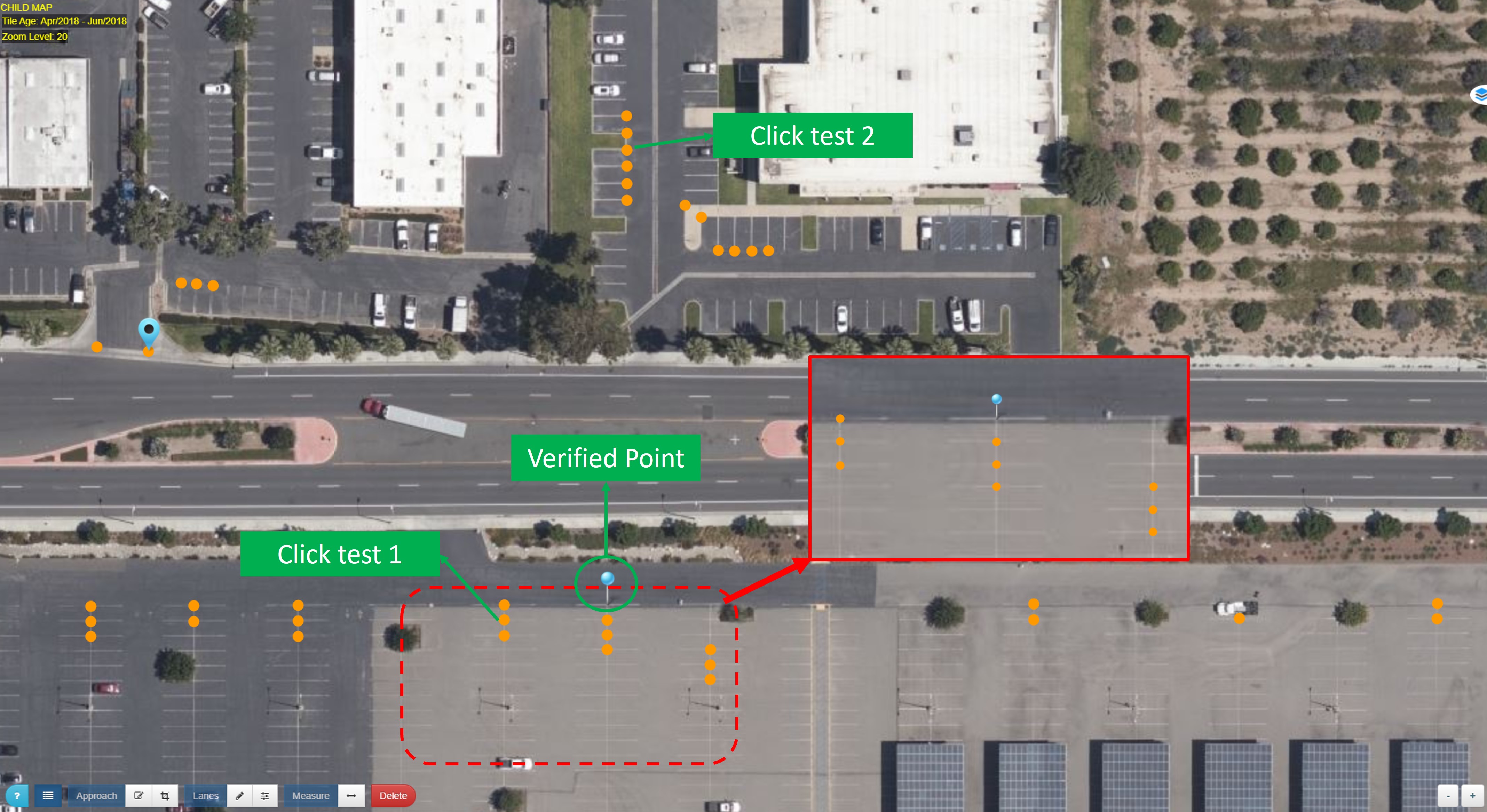
Figure 1: USDOT map accuracy test points near UCR CE-CERT

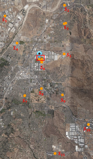
Figure 2: Expanded test area for accuracy analysis.

To assess accuracy, we compare GNSS survey and USDOT mapping tool locations for each feature point. The symbol $\mathbf{P}^{e}$ denotes the feature position determined by GNSS survey. The symbol $\hat{\mathbf{P}}^{e}$ denotes the position of the feature point determined by the USDOT mapping tool. The superscript on the vector $\mathbf{P}$ denotes the frame-of-reference, such as $e$ for ECEF and $g$ for the NED frame. The NED frame feature location of a point ${\mathbf{P}}^{g}$ is computed by

$${\mathbf{P}}^{g}=\mathbf{R}^{g}_{e}\,({\mathbf{P}}^{e}-\mathbf{P}^{e}_{v})$$ (1)

where $\mathbf{P}^{e}_{v}$ is the origin of the NED frame and $\mathbf{R}^{g}_{e}$ is the rotation matrix from the ECEF frame to the NED frame [16]. Eqn. (1) is valid both for GNSS survey and USDOT mapping tool locations.

Section III-A discusses the GNSS survey and assesses its sources of error when determining the coordinates of each point. Section III-B discusses the USDOT tool and assesses its sources of error when determining the coordinates of each point. Section IV combines the USDOT and GNSS data to assess the overall map accuracy.

III-A Data Acquisition: GNSS Survey

This section presents the procedure for determining the real-world position of the verified point and of each feature point (denoted $\mathbf{P}_{k}^{e}$ for $k=1,\ldots,N$) by use of GNSS RTK survey, using a dual-frequency ublox ZED-F9P receiver connected to a dual-band ublox antenna. The antenna is placed on the ground above the corresponding feature point. The receiver communicates with the UCR base station to obtain RTCM corrections and reports RTK fixed position solution in WGS84 ECEF frame.

During the survey process for each point, the ZED-F9P in RTK fixed mode was used to record the position for at least 20 seconds. The mean of these measurements is used in Sec. IV as the surveyed position. The standard deviation of each coordinate in each surveyed position is less than 0.005 m. The RTK GNSS surveyed position MSE, denoted herein as $\sigma_{G}$ at the centimeter level (see e.g., Table 21.7 in [17]).

In addition to the RTK GNSS survey position error characterized by $\sigma_{G}$, there is also antenna placement error due to the fact that the human operator cannot perfectly place the antenna over the feature and account for the antenna phase offset. This error is accounted for by the symbol $\sigma_{S}$ with MSE $\sigma_{S}=0.01\,m$.

III-B Data Acquisition: USDOT Map Tool

The goal of this section is two-fold: (1) to describe the process by which this tool was used to obtain the geodetic coordinates for the selected locations; and (2) to define and assess the related sources of error.

Process. Starting from the URL for the USDOT tool given in Section II, the steps are as follows:

1. In the ISD Message Creator,

   1. Click ‘View Tool’, then under ‘File’ button click ‘New Parent Map’.

   2. Center the map imagery over the region of interest at the ‘Zoom Level 21’, which is the highest resolution, as shown in the inset of Fig. 1.

   3. Click ‘Builder’ from the left bottom corner.

   4. Drag the ‘Verified Point Marker’ to the feature point defined in Section III and shown in Fig. 1. A ‘Verified Point Configuration’ window will automatically open. Input the GNSS survey coordinates for the verified Latitude/Longitude/Elevation.

   5. Drag the ‘Reference Point Marker’ near the verified point in the map. The reference point is required for the tool. It determines the relative position of all feature locations in the J2735 map message, but does not affect the results of the experiments.

2. Under the ‘File’ button from the top menu, select ‘New Child Map’. Click ‘Cancel’ for the popup questions. Use the pencil in the ‘Lanes’ button located near the left bottom corner. Double-click each desired feature location. An orange dot will be displayed as shown Fig. 1.

3. Click the pencil in the ‘Lanes’ button to turn it off. Then, select (i.e., mouse click) each feature point in the tool imagery (e.g., orange points in Fig. 1) and note their coordinates as $\hat{\mathbf{P}}^{e}_{k}$.

Note that all positions acquired from the USDOT tool are WGS84 ECEF geodetic coordinates.

Error Sources. The above process allows measurement error to occur in at least two ways. First, the user will have error in the clicking of points. For example, Steps 1d and 2 involve mouse clicks to select points. At best, the accuracy of such mouse clicks will be the size of the pixel in meters; however, the screen resolution may result in lower accuracy. The click error will be denoted by $\sigma_{C}$. Second, the geodetic coordinates assigned to the clicked points will be imperfect due to georectification errors. This mapping error will be denoted by $\sigma_{M}$.

Error Assessment. The goal of this subsection is to characterize the click accuracy $\sigma_{C}$ in meters. Point-click experiments are performed for two feature points, which are marked as ‘Click test’ in Fig. 1. For each experiment, using ‘Zoom level 21’, the targeted feature point is manually clicked 15 times (moving the cursor away and returning it between clicks) and their position $\hat{\mathbf{P}}^{e}_{C_{i}}$ is recorded for $i=1,...,15$.

The accuracy analysis is performed in a locally-level NED tangent frame with its origin point at the verified position $\hat{\mathbf{P}}^{e}_{v}$. The NED feature location $\hat{\mathbf{P}}^{g}_{C_{i}}$ is computed from $\hat{\mathbf{P}}^{e}_{C_{i}}$ using Eqn. (1).

Herein, click test error is characterized by the STD of each component of ${\mathbf{P}}^{g}_{C_{i}}=[P^{g}_{N_{i}},P^{g}_{E_{i}},P^{g}_{D_{i}}]^{T}$. The STD of North $\sigma_{N}$ and East $\sigma_{E}$ are listed in Table I. The vertical STD $\sigma_{V}$ is 0 since there are no changes in the Down coordinates in each click of each experiment. The horizontal STD, which defines the click accuracy $\sigma_{C}$, is calculated by

$$\sigma_{C}=\sqrt{\sigma_{N}^{2}+\sigma_{E}^{2}}.$$ (2)

The values of $\sigma_{C}$ summarized in Table I, will be used in Section IV-C to estimate a value for $\sigma_{M}$.

TABLE I: Standard deviation for click test

	$\sigma_{N}$	$\sigma_{E}$	$\sigma_{C}$	$\sigma_{V}$
Click test 1	0.053 m	0.028 m	0.060 m	0.0 m
Click test 2	0.042 m	0.032 m	0.053 m	0.0 m

IV Accuracy Assessment

This section uses the USDOT data in comparison with the GNSS survey data to assess the accuracy of the feature locations provided by the USDOT mapping tool.

IV-A Bias Analysis on USDOT Tool: Verified Point

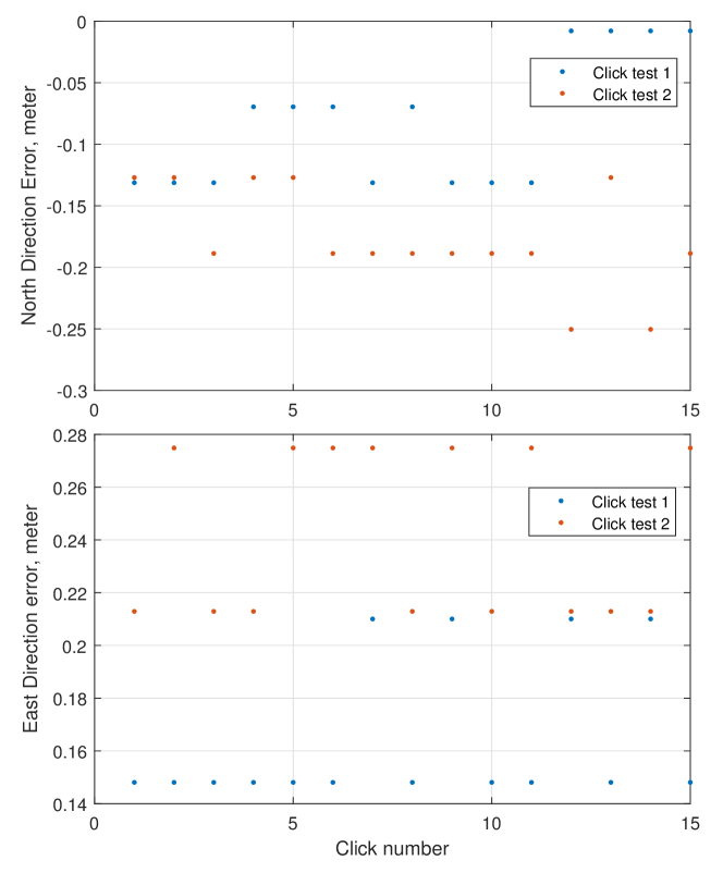
Figure 3: North and east errors between USDOT tool and GNSS survey (i.e, $\delta P^{g}_{N_{i}}$ and $\delta P^{g}_{E_{i}}$ from eqn. (3)) using the two feature points from the click test.

Fig. 3 displays the north and east components of the error between the USDOT feature points from each click test $\hat{\mathbf{P}}^{g}_{C_{i}}$ and the GNSS surveyed positions ${\mathbf{P}}^{g}_{C}$ for the same features. For each click test, the NED frame positions $\hat{\mathbf{P}}^{g}_{C_{i}}$ and ${\mathbf{P}}^{g}_{C}$ are computed using Eqn. (1). The position error is calculated by

$$\delta{\mathbf{P}}^{g}_{C_{i}}={\mathbf{P}}^{g}_{C_{i}}-{\mathbf{P}}^{g}_{C}$$ (3)

where $\delta{\mathbf{P}}^{g}_{C_{i}}=[\delta P^{g}_{N_{i}},\delta P^{g}_{E_{i}},\delta P^{g}_{D_{i}}]^{T}$ are the NED components of mapping error for click test $C_{i}$.

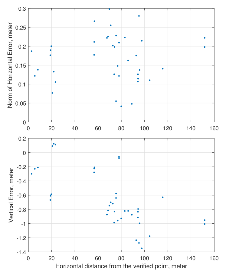
(a) Horizontal error norm $\delta P_{H_{k}}^{g}$ and vertical error $\delta P^{g}_{D_{k}}$
versus HD to the verified point (i.e., $D_{H_{k}}$).

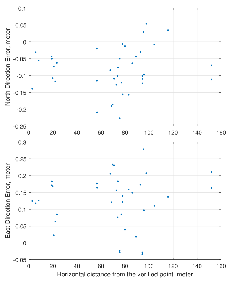
(b) North and East error components versus
HD to the verified point (i.e., $D_{H_{k}}$).

Figure 4: USDOT map accuracy assessment near UCR CE-CERT.

Note that both the north and east components of the position error vector are biased by -0.13 m and 0.21 m, respectively. Due to the fact that the bias is statistically the same for both feature points (i.e., click tests) and all clicks, this bias is attributed to the error in the placement on the verified point within the USDOT tool. See also the discussion of Figs. 4(b) and 5(b).

IV-B Feature Mapping Accuracy Analysis

The USDOT map tool provides geographic coordintes (i.e., Longitude, Latitude, and Altitude) for feature points. The geographic coordinates are transferred to ECEF coordinates using the method described in Eqns. (2.9-2.11) of [18], then to local tangent plane using Eqn. (1). The USDOT location of feature $k$ is denoted as $\hat{\mathbf{P}}^{e}_{k}$ and $\hat{\mathbf{P}}^{g}_{k}$. The GNSS surveyed location of feature $k$ is denoted as ${\mathbf{P}}^{e}_{k}$ and ${\mathbf{P}}^{g}_{k}$. The position error for feature $k$ is computed as

$$\delta\mathbf{P}^{g}_{k}=\hat{\mathbf{P}}^{g}_{k}-{\mathbf{P}}^{g}_{k}=\mathbf{R}^{g}_{e}\,(\hat{\mathbf{P}}^{e}_{k}-\mathbf{P}^{e}_{k})$$

where $\delta\mathbf{P}^{g}_{k}=[\delta P^{g}_{N_{k}},\delta P^{g}_{E_{k}},\delta P^{g}_{D_{k}}]^{T}$ defines the north, east, and down components of the error vector. The metrics for analyzing the accuracy of the $k$-th feature are the horizontal error norm:

$$\delta P_{H_{k}}^{g}=\sqrt{(\delta P^{g}_{N_{k}})^{2}+(\delta P^{g}_{E_{k}})^{2}};$$

and, the vertical error: $\delta P^{g}_{D_{k}}$. The HD between the $k$-th test point and verified point ($\mathbf{P}^{g}_{v}=\bm{0}$) is

$$D_{H_{k}}=\sqrt{(\mathbf{P}^{g}_{N_{k}})^{2}+(\mathbf{P}^{g}_{E_{k}})^{2}}.$$

Fig. 4 displays data for assessing accuracy for the features shown in Fig. 1 that are near CE-CERT. Fig. 4(a) displays the horizontal error norm and vertical error for the feature points near the UCR CE-CERT. Fig. 5 presents data for the expanded area shown in Fig. 2. The expanded area includes 11 clusters. Data for each cluster is depicted in a different color in Fig. 5. In each figure the x-axis is the horizontal distance $D_{H_{k}}$ from the verified point. Fig. 4(a) shows 0.17 m mean and 0.30 m maximum horizontal error. Fig. 5(a) shows the horizontal error norm and vertical errors over longer horizontal distances from the verified point. Fig. 5(a) shows 0.18 m mean and 0.31 m maximum horizontal error. There are no discernible trends in the horizontal error as a function of the distance from the verified point.

Fig. 5(a) also shows that the vertical error does change as a function of the distance from the verified point. The tool georectifies remote sensing satellite imagery to achieve its accuracy in the horizontal directions. Satellite imagery does not provide depth information; therefore, the underlying vertical accuracy is limited.

Figs. 4(b) and 5(b) show the individual components of the horizontal error. In Fig. 4(b) the mean north and east errors are -0.08 m and 0.12 m, respectively. In Fig. 5(b) the mean north and east errors are -0.08 m and 0.15 m, respectively. These biases are consistent with each other and with those in Fig. 3. This verifies the conclusion that the verified point selected within the USDOT tool is biased by this amount relative to the desired feature point, due to the limited resolution of the imagery in that tool.

The symbol $\sigma_{H}$ represents the MSE of the experimental horizontal position error $\delta P_{H_{k}}^{g}$. The MSE of $\delta P_{H_{k}}^{g}$ is 0.18 m for $N_{1}$ points and 0.20 m for $N_{2}$ points. The MSE $\sigma_{H}$ over all 94 feature points is 0.19 m.

Fig. 6 plots the horizontal and vertical errors versus vertical difference relative to the verified point. The horizontal accuracy remains constant as elevation changes. The vertical error is an order of magnitude larger than the horizontal error and does change with both the horizontal and vertical separation from the reference point.

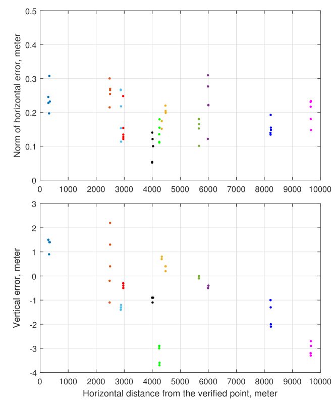
(a) Horizontal error norms and Vertical error

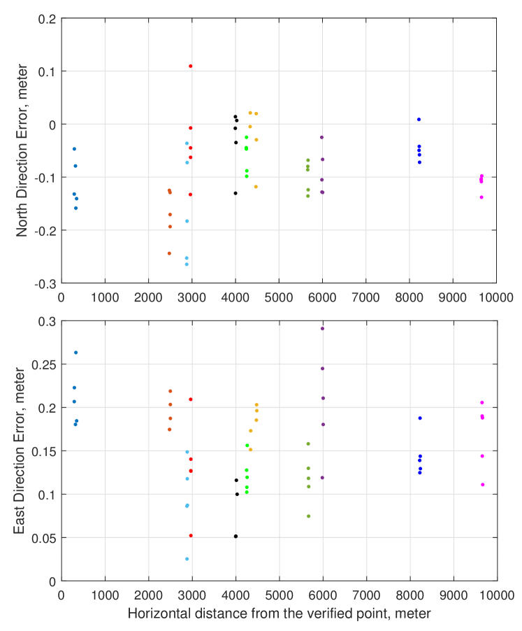
(b) North and East error components

Figure 5: Graphs of USDOT map accuracy assessment for expanded area. $S_{1}$ in green with HD near 5.7 km, $S_{2}$ in dark purple with HD near 6 km, $S_{3}$ in amber with HD near 4.4 km, $S_{4}$ in light blue with HD near 2.9 km, $S_{5}$ in orange with HD near 2.4 km, $S_{6}$ in blue with HD near 0.3 km, $S_{7}$ in black with HD near 4 km, $S_{8}$ in red with HD near 3 km, $S_{9}$ in green with HD near 4.2 km, $S_{10}$ in deep blue with HD near 8.2 km, and $S_{11}$ in magenta with HD near 9.7 km.

IV-C Map Horizontal Accuracy Assessment

The experimental horizontal position error $\sigma_{H}$ is the result of the four specific errors discussed in Sections III-A and III-B, specifically:

$$\sigma_{H}^{2}=2\,\sigma_{C}^{2}+\sigma_{M}^{2}+\sigma_{G}^{2}+\sigma_{S}^{2}.$$

The US-DOT click accuracy $\sigma_{C}$ is multiplied by 2 since it is applied to the clicks for both the feature point and the verified point. Since we have experimentally determined values for $\sigma_{H}$, $\sigma_{C}$, $\sigma_{G}$, and $\sigma_{S}$, we can compute $\sigma_{M}=\sqrt{\sigma_{H}^{2}-\left(2\,\sigma_{C}^{2}+\sigma_{G}^{2}+\sigma_{S}^{2}\right)}$. Using either value of $\sigma_{C}$ from the two click tests, the resulting value of $\sigma_{M}$ is $0.17$ m.

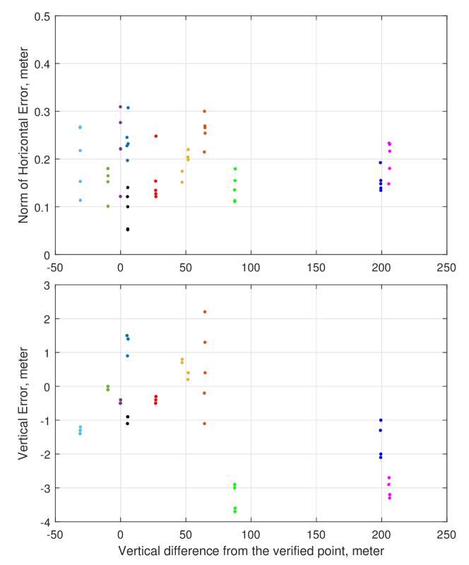
Figure 6: Horizontal error norms and Vertical error of expanded area.

V Conclusions and Discussion

HiD digital maps are an indispensable automated driving technology for CAV applications. The USDOT map tool allows users to create MAP and SPaT messages with free access, but an assessment of its accuracy does not exist in the current literature. This document assessed the accuracy of the US-DOT map tool using a set of 94 feature points with an 10 km area. The assessed mean square horizontal map error is 17 centimeters, which satisfies the lane-level HiD map requirement (10-20 cm) [4]. The maximum horizontal map error is less than 30 centimeters. The assessment also demonstrated that this horizontal map accuracy was maintained within a 10 km distance of the USDOT map tool verified point that was used in this study.

References

- [1] M. White, “Emerging Requirements for Digital Maps for In-Vehicle Pathfinding and Other Traveller Assistance,” in Vehicle Navigation and Information Systems Conference, vol. 2. IEEE, 1991, pp. 179–184.
- [2] K. Massow, B. Kwella, N. Pfeifer, F. Häusler, J. Pontow, I. Radusch, J. Hipp, F. Dölitzscher, and M. Haueis, “Deriving HD maps for highly automated driving from vehicular probe data,” in 19th Int. Conference on Intelligent Transportation Systems (ITSC). IEEE, 2016, pp. 1745–1752.
- [3] J. Jiao, “Machine Learning Assisted High-Definition Map Creation,” in 42nd Annual Computer Software and Applications Conference (COMPSAC), vol. 1. IEEE, 2018, pp. 367–373.
- [4] R. Liu, J. Wang, and B. Zhang, “High definition map for automated driving: Overview and Analysis,” The J. of Navigation, vol. 73, no. 2, pp. 324–341, 2020.
- [5] S. Rogers, P. Langley, and C. Wilson, “Learning to predict lane occupancy using GPS and digital maps,” in Proc. of the 5th Int. Conference on Knowledge Discovery and Data Mining, 1999, pp. 104–113.
- [6] C. Yan, C. Zheng, C. Gao, W. Yu, Y. Cai, and C. Ma, “Lane Information Perception Network for HD Maps,” in 23rd Int. Conference on Intelligent Transportation Systems (ITSC). IEEE, 2020, pp. 1–6.
- [7] V. Potó, Á. Somogyi, T. Lovas, Á. Barsi, V. Tihanyi, and Z. Szalay, “Creating HD map for autonomous vehicles-a pilot study,” in 34th Int. Colloquium on Advanced Manufacturing and Repairing Technologies in Vehicle Industry, 2017.
- [8] J. Lógó, N. Krausz, V. Potó, and A. Barsi, “Quality Aspects of High-Definition Maps,” The Int. Archives of Photogrammetry, Remote Sensing and Spatial Information Sciences, vol. 43, pp. 389–394, 2021.
- [9] B. Pal, S. Khaiyum, Y. Kumaraswamy et al., “Recent advances in Software, Sensors and Computation Platforms Used in Autonomous Vehicles, A Survey,” Int. J. Res. Anal. Rev, vol. 6, no. 1, 2019.
- [10] M. Szántó and L. Vajta, “Introducing crowdmapping: A novel system for generating autonomous driving aiding traffic network databases,” in 2019 Int. Conference on Control, Artificial Intelligence, Robotics & Optimization (ICCAIRO). IEEE, 2019, pp. 7–12.
- [11] M. Abrams and T. Romer, “Eyes on the Road,” Mechanical Engineering, vol. 139, no. 12, pp. 33–33, 2017.
- [12] K. Wong, Y. Gu, and S. Kamijo, “Mapping for Autonomous Driving: Opportunities and Challenges,” IEEE Intell. Transp. Syst. Mag., vol. 13, no. 1, pp. 91–106, 2020.
- [13] C. Hedges and F. Perry, “Overview and use of SAE J2735 message sets for commercial vehicles,” SAE Technical Paper, Tech. Rep., 2008.
- [14] J. B. Kenney, “Dedicated Short-Range Communications (DSRC) Standards in the United States,” Proceedings of the IEEE, vol. 99, no. 7, pp. 1162–1182, 2011.
- [15] H. Topan and H. S. Kutoglu, “Georeferencing accuracy assessment of high-resolution satellite images using figure condition method,” IEEE Transactions on Geoscience and Remote Sensing, vol. 47, no. 4, pp. 1256–1261, 2009.
- [16] W. Hu, A. Neupane, and J. A. Farrell, “Using PPP Information to Implement a Global Real-Time Virtual Network DGNSS Approach,” arXiv preprint arXiv:2110.14763, 2021.
- [17] P. Teunissen and O. Montenbruck, Springer Handbook of Global Navigation Satellite Systems. Springer, 2017.
- [18] J. A. Farrell, Aided Navigation: GPS with High Rate Sensors. McGraw-Hill, Inc., 2008.