Detecting and Eliminating Quantum Noise of Quantum Measurements

Abstract

Quantum measurements are crucial for extracting information from quantum systems, but they are error-prone due to hardware imperfections in near-term devices. Measurement errors can be mitigated through classical post-processing, based on the assumption of a classical noise model. However, the coherence of quantum measurements leads to unavoidable quantum noise that defies this assumption. In this work, we introduce a two-stage procedure to systematically tackle such quantum noise in measurements. The idea is intuitive: we first detect and then eliminate quantum noise. In the first stage, inspired by coherence witness in the resource theory of quantum coherence, we design an efficient method to detect quantum noise. It works by fitting the difference between two measurement statistics to the Fourier series, where the statistics are obtained using maximally coherent states with relative phase and maximally mixed states as inputs. The fitting coefficients quantitatively benchmark quantum noise. In the second stage, we design various methods to eliminate quantum noise, inspired by the Pauli twirling technique. They work by executing randomly sampled Pauli gates before the measurement device and conditionally flipping the measurement outcomes in such a way that the effective measurement device contains only classical noise. We numerically demonstrate the two-stage procedure’s feasibility on the Baidu Quantum Platform. Notably, the results reveal significant suppression of quantum noise in measurement devices and substantial enhancement in quantum computation accuracy. We highlight that the two-stage procedure complements existing measurement error mitigation techniques, and they together form a standard toolbox for manipulating measurement errors in near-term quantum devices.

I Introduction

Quantum computers offer significant potential across scientific and industrial domains. However, the current noisy intermediate-scale quantum (NISQ) computers [1] introduce notable errors, necessitating their mitigation prior to engaging in practically valuable endeavors. These errors emerge from either undesired qubit-environment interactions or the physical imperfections inherent in qubit initializations, quantum gates, and measurements [2, 3, 4, 5]. Typically, errors in a quantum computer are categorized into quantum gate errors and measurement errors. For the former, various quantum error mitigation techniques have been proposed to mitigate the damages caused by errors on near-term quantum devices  [6, 7, 8, 9, 10, 11, 12, 13, 14, 15, 16, 17, 18, 19, 20, 21]. For the latter, most experiments work with the assumption that measurement errors in quantum devices are well understood in terms of classical noise models [22, 23, 24]. Specifically, an $n$-qubit noisy measurement device can be characterized by a noise matrix of size $2^{n}\times 2^{n}$. The element in the $\bm{x}$-th row and $\bm{y}$-th column of the matrix is the probability of obtaining an outcome $\bm{x}$ provided that the true outcome is $\bm{y}$. If one has access to this stochastic matrix, it is straightforward to classically reverse the noise effects simply by multiplying the probability vector obtained from measurement statistics by this matrix’s inversion or its approximations, known as the measurement error mitigation [25, 26, 27, 28, 29, 30, 31, 32, 33, 34, 35, 36, 21].

From the perspective of positive operator-valued measure (POVM) formalism, the classical noise model indicates that the POVM elements characterizing the measurement device possess only non-zero diagonal values with respect to (w.r.t.) the computational basis. However, due to the coherent nature of quantum mechanics incurred during calibration and/or interaction, the POVM elements signalizing a near-term measurement device necessarily have off-diagonal non-zero values, which is called coherence in the resource theory of quantum coherence [37]. That is to say, the coherence effect can be seen as one of the sources of measurement imperfections. This coherence effect renders the behavior of measurement devices unpredictable. Complete information regarding these devices can only be obtained through exponentially resource-intensive quantum detector tomography [38, 39]. Furthermore, this observation prompts the realization that existing measurement error mitigation techniques could be enhanced, as the classical noise model assumption fails to consider the influence of quantum noise. Consequently, we describe a measurement device as afflicted by quantum noise when its POVM elements encompass non-zero off-diagonal values. This leads us to the fundamental query of how to effectively address this form of noise.

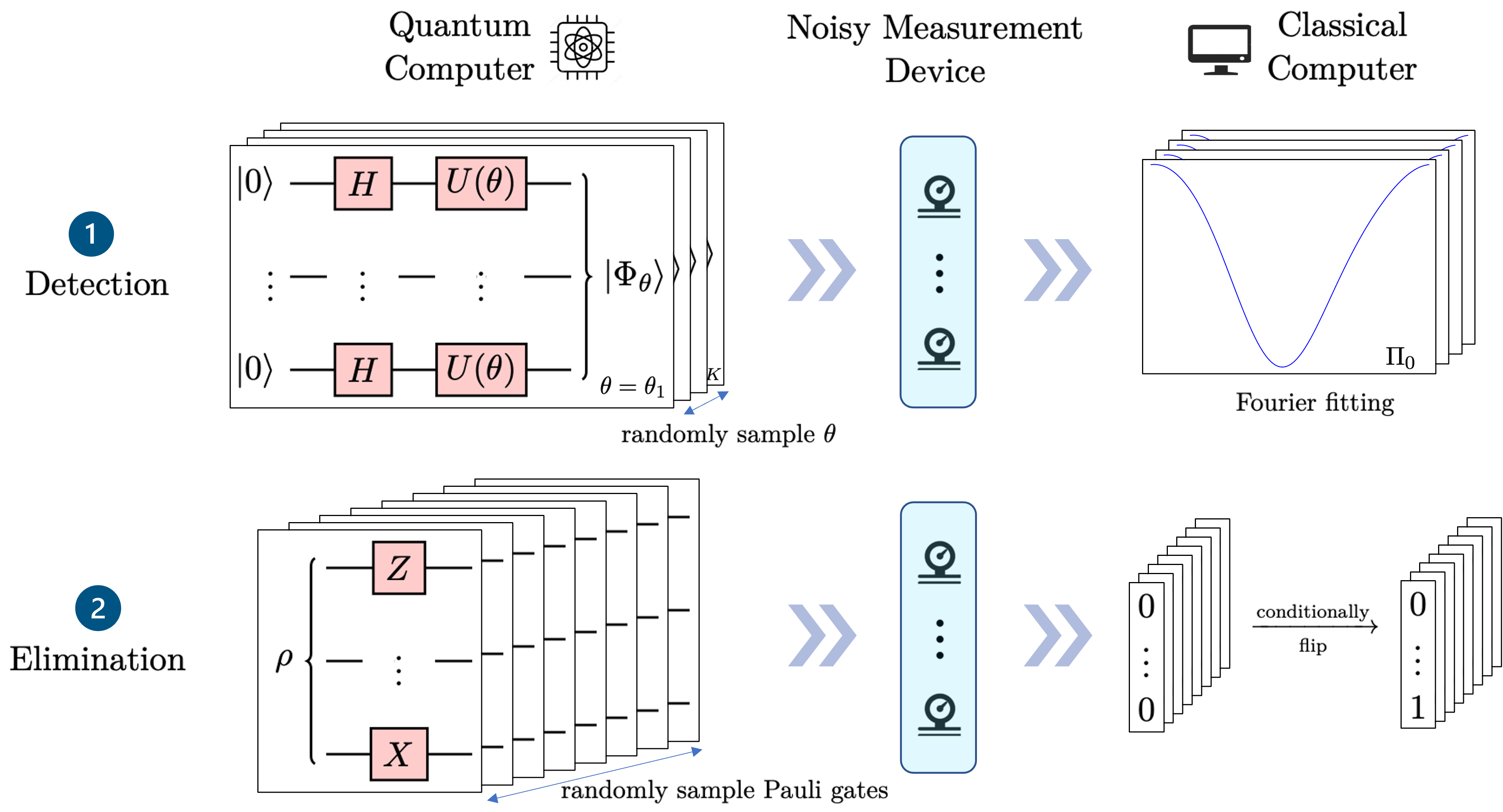
Figure 1: A two-stage procedure for detecting and eliminating quantum noise of quantum measurement devices. In the first stage, we prepare maximally coherent states $|\Phi_{\theta}\rangle$ with relative phase $\theta$ and maximally mixed states as inputs, and fit the difference between two measurement statistics to the Fourier series. The fitting coefficients quantitatively benchmark quantum noise. In the second stage, we execute randomly sampled Pauli gates before the measurement device and conditionally flip the outcomes, in such a way that the resulting effective measurement contains only classical noise.

In this work, we propose a two-stage procedure to systematically address quantum noise inherent in NISQ measurement devices. The procedure is illustrated in Figure 1 and is very intuitive: we first detect and then eliminate quantum noise if there is any. It is noteworthy that the detection process is efficient, while the elimination process is resource-consuming. Consequently, prioritizing the detection of quantum noise is advisable. After the procedure, the classical noise model assumption is obviously satisfied and the classical noise can be diminished using measurement error mitigation. The rest of the paper is organized as follows. Section II sets the notation and introduces the task of addressing quantum noise inherent in quantum measurements. Section III elaborates the procedure’s first stage, which proposes an efficient method to detect the quantum noise of measurement devices. Section IV elaborates the procedure’s second stage by describing three different methods to eliminate the quantum noise of measurement devices. Section V reports the feasibility of the proposed two-stage procedure numerically on Baidu Quantum Platform [40] with three paradigmatic quantum applications. The Appendices summarize technical details used in the main text.

II Preliminaries

In this section, we first set the notations. Then, we review different yet equivalent mathematical formalisms of quantum measurements. Finally, we rigorously define the classical and quantum noises of a quantum measurement device.

II.1 Notations

For a finite-dimensional Hilbert space $\mathcal{H}$, we denote by $\mathscr{L}(\mathcal{H})$ and $\mathscr{P}(\mathcal{H})$ the linear and positive semidefinite operators on $\mathcal{H}$. Quantum states are in the set $\mathscr{D}(\mathcal{H})\mathrel{\mathop{\mathchar 58\relax}}=\{\rho\in\mathscr{P}(\mathcal{H})|\operatorname{Tr}\rho=1\}$. For two operators $M,N\in\mathscr{L}(\mathcal{H})$, we say $M\geq N$ if and only if $M-N\in\mathscr{P}(\mathcal{H})$. The identity matrix is denoted as $\mathbbm{1}$, the maximally mixed state is denoted as $\Pi$, and the diagonal column vector of an operator $M$ w.r.t. the computational basis is denoted as $\operatorname{diag}(M)$. Multipartite quantum systems are described by tensor product spaces. Denote by $\mathbb{C}$, $\mathbb{R}$, and $\mathbb{R}^{+}$ the complex, real, and non-negative real numbers, respectively. In this paper, we assume $\mathcal{H}_{n}$ represents the $n$-qubit Hilbert space and our attention focuses on investigating classical and quantum noises of measurements in this space.

II.2 Quantum measurements

The most general kind of measurements in quantum mechanics is called positive operator-valued measures (POVMs). A POVM is a set of operators $\{E_{\bm{x}}\}_{\bm{x}\in\Sigma}$ satisfying $\forall\bm{x},E_{\bm{x}}\geq 0$ and $\sum_{\bm{x}}E_{\bm{x}}=\mathbbm{1}$, where $\Sigma$ is an alphabet and $\bm{x}\in\Sigma$ records the measurement outcome [41]. If one performs the POVM $\{E_{\bm{x}}\}$ on a quantum state $\rho$, the probability of obtaining outcome $\bm{x}$ is given by the Born’s rule

$$p(\bm{x})\mathrel{\mathop{\mathchar 58\relax}}=\operatorname{Tr}[E_{\bm{x}}\rho].$$ (1)

Notice that in the POVM representation, we do not care about the post-measurement state but only care about the probability of obtaining a particular outcome. We fix $\Sigma=\{0,1\}^{n}$ in the following discussion.

In Quantum Information Theory, researchers commonly think of measurements from the quantum channel viewpoint by regarding the post-measurement states as purely classical states. Mathematically, the induced measurement channel of a POVM $\{E_{\bm{x}}\}_{\bm{x}\in\Sigma}$ is defined as [42]

$$\mathcal{M}(\rho)\mathrel{\mathop{\mathchar 58\relax}}=\sum_{\bm{x}\in\Sigma}\operatorname{Tr}\left[E_{\bm{x}}\rho\right]|{\bm{x}}\rangle\!\langle{\bm{x}}|,$$ (2)

where $\{\left|{\bm{x}}\right\rangle\}_{\bm{x}\in\Sigma}$ is the computational basis of the underlying Hilbert space. Notice that a measurement channel takes a quantum system to a classical one.

The Pauli transfer matrix (PTM) representation is intensively used to notate quantum states and quantum processes in tomography tasks [43]. In PTM, an $n$-qubit quantum channel is represented by a $4^{n}\times 4^{n}$ real matrix defined w.r.t. vectorization in the Pauli basis instead of column-vectorization. Specifically, the PTM matrix $[\mathcal{M}]$ of the measurement channel $\mathcal{M}$ defined in (2) has the form

$$[\mathcal{M}]_{\bm{i}\bm{j}}\mathrel{\mathop{\mathchar 58\relax}}=\frac{1}{2^{n}}\operatorname{Tr}[P_{\bm{i}}\mathcal{M}(P_{\bm{j}})]=\frac{1}{2^{n}}\sum_{\bm{x}\in\Sigma}\operatorname{Tr}[E_{\bm{x}}P_{\bm{j}}]\langle\bm{x}|P_{\bm{i}}|\bm{x}\rangle,$$ (3)

where $[\mathcal{M}]_{\bm{i}\bm{j}}$ is the element in the $\bm{i}$-th row $\bm{j}$-th column and $P_{\bm{i}}\in\mathsf{P}^{n}$ is the $\bm{i}$-th Pauli operator (sorted by lexicographic order) in the $n$-qubit Pauli set $\mathsf{P}^{n}\mathrel{\mathop{\mathchar 58\relax}}=\{I,X,Y,Z\}^{\otimes n}$.

Given the POVM representation $\{E_{\bm{x}}\}_{\bm{x}\in\Sigma}$, we can compute the PTM representation via Eq. (3). In the following, we give a method to compute the POVM representation given the PTM representation $[\mathcal{M}]$. The proof is given in Appendix E.

Proposition 1.

Let $[\mathcal{M}]$ be the PTM representation of an arbitrary unknown POVM $\{E_{\bm{x}}\}_{\bm{x}\in\Sigma}$. It holds for arbitrary $\bm{x}\in\Sigma$ that

$$E_{\bm{x}}=\frac{1}{2^{n}}\sum_{P_{\bm{i}},P_{\bm{j}}\in\mathsf{P}^{n}}\left\langle{\bm{x}}\right|P_{\bm{i}}\left|{\bm{x}}\right\rangle[\mathcal{M}]_{\bm{i}\bm{j}}P_{\bm{j}}.$$ (4)

Throughout this paper we use the POVM representation $\{E_{\bm{x}}\}_{\bm{x}\in\Sigma}$, the measurement channel representation $\mathcal{M}$, and the PTM representation $[\mathcal{M}]$ interchangeably. The representations of symbols should be clear from context.

II.3 Classical and quantum noises

In most existing quantum computing platforms [3, 15, 44], measurement devices are designed to implement an ideal $n$-qubit computational basis measurement, also called the $Z$ measurement, whose POVM $\{E_{\bm{x}}^{i}\}_{\bm{x}}$ has the form

$$\forall\bm{x}\in\{0,1\}^{n},\quad E_{\bm{x}}^{i}=|{\bm{x}}\rangle\!\langle{\bm{x}}|,$$ (5)

where the superscript $i$ means ideal and $\{\left|{\bm{x}}\right\rangle\}_{\bm{x}\in\{0,1\}^{n}}$ is the computational basis of an $n$-qubit Hilbert space. Note that $E_{\bm{x}}^{i}$ is a $2^{n}\times 2^{n}$ matrix with $1$ in the $\bm{x}$-row and $\bm{x}$-column and $0$ in all other cells.

Practically, the measurement apparatus is imperfect and introduces different kinds of noises. In order to simplify the post-processing, experimenters commonly assume that the incurred noises are well understood in terms of classical noise models [22, 25, 23, 24]. In the POVM language, we say a POVM $\{E_{\bm{x}}^{c}\}_{\bm{x}\in\{0,1\}^{n}}$ (the superscript $c$ means classical) that characterizes a measurement device is classical if, besides $E_{\bm{x}}^{c}\geq 0$ and $\sum_{\bm{x}}E^{c}_{\bm{x}}=\mathbbm{1}$, it satisfies two more conditions: 1) the off-diagonal elements of all $E_{\bm{x}}^{c}$ are zero, i.e., $\forall\bm{y}\neq\bm{z}$, $\left\langle{\bm{y}}\right|E_{\bm{x}}\left|{\bm{z}}\right\rangle=0$, $\forall\bm{x}$; and 2) there exists at least one $E_{\bm{x}}^{c}$ whose diagonal elements contain more than one non-zero values, i.e., $\exists\bm{x},\bm{y}$ such that $\bm{x}\neq\bm{y}$ and $\left\langle{\bm{y}}\right|E_{\bm{x}}\left|{\bm{y}}\right\rangle\neq 0$. Experimentally, this means that when we input the computational basis state $\left|{\bm{x}}\right\rangle$ to the measurement device, we have some probability of obtaining an incorrect measurement outcome $\bm{y}$. If the measurement is classical, we call its induced measurement channel a classical measurement channel. We can use calibration to learn parameters of a classical measurement from experimental data and error mitigation methods to diminish classical noise [28, 26, 27, 29, 30, 31, 32, 33, 34, 35, 36, 21].

In the most general case, the POVM $\{E_{\bm{x}}^{q}\}_{\bm{x}\in\{0,1\}^{n}}$ (the superscript $q$ means quantum) that characterizes a noisy measurement device only need to satisfy the fundamental conditions $E_{\bm{x}}^{q}\geq 0$ and $\sum_{\bm{x}}E^{q}_{\bm{x}}=\mathbbm{1}$. Thus, $E_{\bm{x}}^{q}$ can have non-zero values in both diagonal and off-diagonal parts. We term the non-zero values in the diagonal part as classical noise and the non-zero values in the off-diagonal part as quantum noise. We can use quantum detector tomography to learn parameters of a general POVM from experimental data [38, 39], which is both time consuming and computationally difficult. The bitter truth is that in tomography, a few-qubit measurement device is already experimentally challenging. What’s worse, none of the mentioned mitigation methods can be applied to cancel the effect of quantum noise. In the following, we propose a two-stage procedure to first detect and then eliminate quantum noise. After the procedure, only classical noise remains, and we can use mitigation methods to handle them.

III Quantum noise detection

In this section, we describe the first stage of the quantum noise manipulating procedure by proposing an efficient quantum noise detection method. To commence, we introduce the notion of quantum noise witnesses, which we define as quantum observables that comprehensively capture classical noise attributes and enable the physical identification of quantum noise. Subsequently, leveraging the direct measurability of quantum noise witnesses, we propose a Fourier series fitting method to detect quantum noise quantitatively. Ultimately, we validate the efficacy of this fitting methodology through numerical verification conducted on the Baidu Quantum Platform.

III.1 Quantum noise witness

III.1.1 Definition

In brief, a quantum noise witness is a function designed to differentiate a particular quantum POVM element from classical POVM elements. These witnesses draw inspiration from quantum entanglement witnesses [45, 46] and are rooted in geometry: the convex sets of classical POVM elements can be delineated using hyperplanes.

Definition 2 (Quantum noise witness).

Let $W$ be a Hermitian operator in $\mathcal{H}_{n}$. $W$ is called a quantum noise witness, if

1. for arbitrary classical POVM $\{E^{c}_{\bm{x}}\}_{\bm{x}}$, it holds for arbitrary $\bm{x}$ that $\operatorname{Tr}[WE^{c}_{\bm{x}}]=0$;

2. there exists at least one quantum POVM $\{E^{q}_{\bm{x}}\}_{\bm{x}}$ such that there exists some $\bm{x}$ for which $\operatorname{Tr}[WE^{q}_{\bm{x}}]\neq 0$.

Thus, if one measures $\operatorname{Tr}[WE_{\bm{x}}]\neq 0$ for some $E_{\bm{x}}$, one knows for sure that this POVM element, and the corresponding POVM, is witnessed by $W$ and contains quantum noise.

Notice that our definition of quantum noise witness differs slightly from the standard definition used by entanglement witnesses. The separation hyperplane is determined by the expectation values equaling $0$. In Appendix A, we elaborate that these two definitions are equivalent.

Motivated by the intuition that the operators close to a maximally coherent state must possess non-zero off-diagonal values [37], one can construct a quantum noise witness from a given pure coherent quantum state $\left|{\psi}\right\rangle\mathrel{\mathop{\mathchar 58\relax}}=\sum_{\bm{y}}c_{\bm{y}}\left|{\bm{y}}\right\rangle$, where $c_{\bm{y}}\in\mathbb{C}$, via

$$W_{\psi}\mathrel{\mathop{\mathchar 58\relax}}=\alpha\mathbbm{1}-|{\psi}\rangle\!\langle{\psi}|,$$ (6)

where $\alpha\in\mathbb{R}^{+}$ is to be determined. We call $\psi$ the probe state and $W_{\psi}$ the $\psi$-induced quantum noise witness. The parameters $\{c_{\bm{y}}\}_{\bm{y}}$ and $\alpha$ must be chosen to ensure that $W_{\psi}$ satisfies Condition 1. Notice that

$$\operatorname{Tr}\left[W_{\psi}E_{\bm{x}}\right]=\sum_{\bm{y}}(\alpha-|c_{\bm{y}}|^{2})E_{\bm{x}}(\bm{y},\bm{y})-\sum_{\bm{y}\neq\bm{z}}c_{\bm{y}}^{\ast}c_{\bm{z}}E_{\bm{x}}(\bm{y},\bm{z}),$$ (7)

where $A(\bm{y},\bm{z})$ is the element of $A$ in the $\bm{y}$-th row and $\bm{z}$-th column and $c^{\ast}$ is the complex conjugate of $c$. To ensure Condition 1, the first term in the RHS. of (7) must evaluate to $0$ for arbitrary classical $E_{\bm{x}}$, which holds if and only if $|c_{\bm{y}}|^{2}=\alpha$ for arbitrary $\bm{y}$. This leads to $\alpha=1/2^{n}$ and $c_{\bm{y}}=e^{i\theta_{\bm{y}}}/\sqrt{2^{n}}$ for some $\theta_{\bm{y}}\in[0,2\pi]$, thanks to the normalization condition. Correspondingly, the Hermitian operator

$$W_{\psi}=\frac{1}{2^{n}}\mathbbm{1}-|{\psi}\rangle\!\langle{\psi}|$$ (8)

witnesses the quantum noise of a given POVM via the expectation value

$$\operatorname{Tr}\left[W_{\psi}E_{\bm{x}}\right] =-\frac{1}{2^{n}}\sum_{\bm{y}\neq\bm{z}}e^{i(\theta_{\bm{z}}-\theta_{\bm{y}})}E_{\bm{x}}(\bm{y},\bm{z}).$$ (9)

Since $E_{x}$ is positive semidefinite, the RHS. of (9) must be real. If $E_{\bm{x}}$ is classical then $\operatorname{Tr}\left[W_{\psi}E_{\bm{x}}\right]=0$. Thus $\operatorname{Tr}\left[W_{\psi}E_{\bm{x}}\right]\neq 0$ implies that $E_{\bm{x}}$ possesses quantum noise. It is not hard to find out that the quantum noise witness scheme can be easily realized through constructing special quantum states.

Since the expectation value of an observable depends linearly on the operator, the set of POVM elements is cut into two parts by the expectation value $\operatorname{Tr}[W_{\psi}E]$. In part with $\operatorname{Tr}[W_{\psi}E]=0$ lies the set of all classical POVM elements and some quantum POVM elements that can not be detected by $W_{\psi}$, while the other part $\operatorname{Tr}[W_{\psi}E]\neq 0$ lies the set of quantum POVM elements detected by $W_{\psi}$. From this geometrical interpretation, it follows that all quantum POVMs can be detected by quantum noise witnesses of the form $W_{\psi}$ (8). The proof is given in Appendix B.

Proposition 3 (Completeness).

For arbitrary quantum POVM element $E^{q}$, there exists a probe state $\psi$ for which the $\psi$-induced quantum noise witness $W_{\psi}$ (8) detects $E^{q}$.

Furthermore, as evident from Eq. (9), the $\psi$-induced quantum noise witness $W_{\psi}$ can not only detect but also quantitatively measure the quantum noise of the noisy measurements to some degree. Inspired by this observation, we propose the following quantum noise measure.

Definition 4 ($\psi$-induced quantum noise measure).

Let $\bm{E}\equiv\{E_{\bm{x}}\}_{\bm{x}\in\{0,1\}^{n}}$ be a POVM in $\mathcal{H}_{n}$. The $\psi$-induced quantum noise measure of $E_{\bm{x}}$ is defined as

$$\mathscr{Q}_{\psi}(E_{\bm{x}})\mathrel{\mathop{\mathchar 58\relax}}=2^{n}|\operatorname{Tr}[W_{\psi}E_{\bm{x}}]|.$$ (10)

The (average) quantum noise measure of $\bm{E}$ is defined as

$$\mathscr{Q}_{\psi}(\bm{E})\mathrel{\mathop{\mathchar 58\relax}}=\frac{1}{2^{n}}\sum_{\bm{x}}\mathscr{Q}_{\psi}(E_{\bm{x}}).$$ (11)

In Appendix C, we elaborate on the $\psi$-induced quantum noise measure $\mathscr{Q}_{\psi}$ in depth by investigating its general properties, the analytical solution in the qubit case, and its relations to the resource theory of quantum measurements [47].

III.1.2 Concrete case

Although Proposition 3 ensures that any quantum noise in POVM can in principle be detected by some quantum noise witness, the challenge lies in constructing good witnesses that can detect as many quantum POVMs as possible. In this section, we specialize a probe state and introduce a single-parameter quantum noise witness family that can quantitatively gauge the quantum noise strength of quantum POVMs.

We first define the following $n$-qubit maximally coherent quantum state

$$\left|{\Phi_{\theta}}\right\rangle\mathrel{\mathop{\mathchar 58\relax}}=\left|{+_{\theta}}\right\rangle^{\otimes n},$$ (12)

where the single-qubit state $\left|{+_{\theta}}\right\rangle$ is defined as

$$\left|{+_{\theta}}\right\rangle\mathrel{\mathop{\mathchar 58\relax}}=\frac{\left|{0}\right\rangle+e^{i\theta}\left|{1}\right\rangle}{\sqrt{2}}=\frac{1}{\sqrt{2}}\begin{bmatrix}1\\ e^{i\theta}\end{bmatrix}$$ (13)

and can be obtained by applying the Hadamard gate followed by a phase shift gate $R_{\theta}\mathrel{\mathop{\mathchar 58\relax}}=\begin{bmatrix}1&0\\ 0&e^{i\theta}\end{bmatrix}$. Using $\Phi_{\theta}$ as a probe state, the induced quantum noise witnesses have the form

$$W_{\Phi}^{\theta}\mathrel{\mathop{\mathchar 58\relax}}=\frac{1}{2^{n}}\mathbbm{1}-|{\Phi_{\theta}}\rangle\!\langle{\Phi_{\theta}}|.$$ (14)

Remarkably, we find that the $\Phi_{\theta}$-induced quantum noise measure $\mathscr{Q}_{\Phi}^{\theta}(E_{\bm{x}})\mathrel{\mathop{\mathchar 58\relax}}=2^{n}|\operatorname{Tr}[W_{\Phi}^{\theta}E_{\bm{x}}]|$ has an elegant expression in the form of the sine-cosine Fourier series, where the coefficients are completely determined by the real and imaginary parts of $E_{\bm{x}}$’s off-diagonal elements. We summarize this exciting finding in the following theorem and give its proof in Appendix D.

Theorem 5.

Let $\bm{E}=\{E_{\bm{x}}\}_{\bm{x}\in\{0,1\}^{n}}$ be a POVM in $\mathcal{H}_{n}$. For arbitrary $\bm{x}$, it holds that

$$\mathscr{Q}_{\Phi}^{\theta}\left(E_{\bm{x}}\right) =2\left|\sum_{\bm{y<z}}\bigg{(}-\Re\left[E_{\bm{x}}(\bm{y},\bm{z})\right]\cos\left[h(\bm{y},\bm{z})\theta\right]\right.$$

$$\qquad\qquad\;\;\left.+\Im\left[E_{\bm{x}}(\bm{y},\bm{z})\right]\sin\left[h(\bm{y},\bm{z})\theta\right]\bigg{)}\right|,$$ (15)

where $\Re\left(x\right)$ and $\Im\left(x\right)$ represent the real and imaginary part of a complex number $x$, respectively, $h(\bm{y},\bm{z})\mathrel{\mathop{\mathchar 58\relax}}=\left|\bm{y}\right|-\left|\bm{z}\right|$, and $|\bm{y}|$ represents the Hamming weight of $\bm{y}$.

The key idea behind the elegant form of $\mathscr{Q}_{\Phi}^{\theta}\left(E_{\bm{x}}\right)$ is that the probe state yields an orthogonal basis of the trigonometric functions:

$$\left\{\cos[h(\bm{y},\bm{z})\theta],\sin[h(\bm{y},\bm{z})\theta]\mathrel{\mathop{\mathchar 58\relax}}h(\bm{y},\bm{z})\in\left[0,\cdots,n\right]\right\},$$ (16)

where $n$ denotes the number of qubits. The off-diagonal parts of each POVM element can be expanded in the basis, and the coefficients are the sum over off-diagonal elements that have the same Hamming weight difference $h$. The detection ability of $\mathscr{Q}_{\Phi}^{\theta}\left(E_{\bm{x}}\right)$ is completely determined by the basis. For example, the $2$-qubit quantum noise witness $W_{\Phi}^{\theta}$ has the form

$$W_{\Phi}^{\theta}=\frac{1}{4}\left[\begin{array}[]{cccc}0&-e^{-i\theta}&-e^{-i\theta}&-e^{-i2\theta}\\ -e^{i\theta}&0&-1&-e^{-i\theta}\\ -e^{i\theta}&-1&0&-e^{-i\theta}\\ -e^{i2\theta}&-e^{i\theta}&-e^{i\theta}&0\end{array}\right].$$ (21)

When $h=1$, the real and imaginary components of $\left\langle{01}\right|E_{\bm{x}}\left|{00}\right\rangle$, $\left\langle{10}\right|E_{\bm{x}}\left|{00}\right\rangle$, $\left\langle{11}\right|E_{\bm{x}}\left|{01}\right\rangle$ and $\left\langle{11}\right|E_{\bm{x}}\left|{10}\right\rangle$ as well as their conjugates would be expanded as the coefficients of $\cos{(\theta)}$ and $\sin{(\theta)}$ respectively.

Consider a special case of $\mathscr{Q}_{\Phi}^{\theta}$ by choosing $\theta=0$:

$$\mathscr{Q}_{\Phi}^{\theta=0}\left(E_{\bm{x}}\right) =\left|-2\sum_{\bm{y}<\bm{z}}\Re\left[E_{\bm{x}}\left({\bm{y},\bm{z}}\right)\right]\right|.$$ (22)

Interestingly, it records the sum of the real parts of all off-diagonal values of $E_{\bm{x}}$. If $\mathscr{Q}_{\Phi}^{\theta=0}\left(E_{\bm{x}}\right)\neq 0$, we can conclude safely that $E_{\bm{x}}$ possesses quantum noise, though the converse statement is not necessarily true.

III.2 Efficient detection

The fact that $\psi$-induced quantum noise witnesses and measures are directly measurable quantities makes them appealing for detecting quantum noise in measurement devices from the experiment perspective. Specifically, to implement the quantum noise witness $W_{\Phi}^{\theta}$, defined in Eq. (14), for some fixed $\theta$, we suffice to prepare many copies of quantum states—the maximally mixed state $\Pi\mathrel{\mathop{\mathchar 58\relax}}=\mathbbm{1}/2^{n}$ and the maximally coherent state $\Phi_{\theta}$—and feed them to the noisy measurement device. The expectation value $\operatorname{Tr}[W_{\Phi}^{\theta}E_{\bm{x}}]$ can be easily estimated from the measurement statistics via classical postprocessing. Furthermore, after we successfully estimate $\operatorname{Tr}[W_{\Phi}^{\theta}E_{\bm{x}}]$ for many different values of $\theta$, we can fit these expectation values to a Fourier series. It is clear from Eq. (5) that the obtained fitting coefficients quantitatively characterize the real and imaginary parts of the POVM element under consideration. The whole quantum noise detection procedure is outlined in Algorithm 1.

Algorithm 1 Quantum noise detection

0:  $\bm{E}$: the $n$-qubit measurement device,      $K$: number of phase values $\theta$ to be sampled,      $N_{\rm shots}$: number of measurement shots.

0:  Coefficients that quantify $\bm{E}$’s quantum noise strength.

1:  for $k=1,\cdots,K$ do

2:     Randomly sample a phase $\theta_{k}\in[0,2\pi]$;

3:     Generate $N_{\rm shots}$ number of copies of the $n$-qubit maximally coherent state $\Phi_{\theta}$ with relative phase $\theta_{k}$;

4:     Perform the device $\bm{E}$ on the above quantum states and record the number of occurrences $N_{\bm{x}}^{\theta_{k}}$ of outcome $\bm{x}$;

5:     Generate $N_{\rm shots}$ number of copies of the $n$-qubit maximally mixed state $\Pi$;

6:     Perform the device $\bm{E}$ on the above quantum states and record the number of occurrences $M_{\bm{x}}$ of outcome $\bm{x}$;

7:     For every $\bm{x}\in\{0,1\}^{n}$, estimate the expectation value

$$\hat{\mathscr{Q}}_{\Phi}^{\theta_{k}}(E_{\bm{x}})=2^{n}(M_{\bm{x}}-N_{\bm{x}}^{\theta_{k}})/N_{\rm shots},$$

where the overhat indicates that it is an estimate.

8:  end for

9:  For every $\bm{x}\in\{0,1\}^{n}$, fit the data $\{\hat{\mathscr{Q}}_{\Phi}^{\theta_{k}}(E_{\bm{x}})\mathrel{\mathop{\mathchar 58\relax}}k=1,\cdots,K\}$ to a Fourier series and obtain the fitting coefficients for $E_{\bm{x}}$.

10:  Output all the fitting coefficients.

Now we analyze the sample complexity—the number of copies of quantum states consumed—of Algorithm 1. Obviously, a total of $2KN_{\rm shots}$ number of copies of quantum states has to be prepared and measured. The critical question is, how large $N_{\rm shots}$ should be so that the expectation value $\mathscr{Q}_{\Phi}^{\theta_{k}}(E_{\bm{x}})$ for given $\theta_{k}$ and $\bm{x}$ can be estimated to the desired precision $\varepsilon$?

Each measurement gives a probability $X_{i}$, then $\bar{X}=\frac{1}{N_{\rm shots}}(X_{1}+\dots+X_{N_{\rm shots}})$, and $\operatorname{E}[\bar{X}]=\operatorname{Tr}[E_{x}\Phi_{\theta}^{k}]$. Each $X_{i}$ satisfies $X_{i}\in[0,1]$. Then from Hoeffding’s inequality, we can have, for all $\epsilon\geq 0$,

$$\operatorname{Pr}(|\bar{X}-\operatorname{E}[\bar{X}]|\geq\epsilon)\leq 2\exp{(-2N_{\rm shots}\epsilon^{2})}.$$ (23)

Introduce failure probability $\delta$, we can obtain that

$$2\exp{(-2\epsilon^{2}/N_{\rm shots})}\leq\delta.$$ (24)

Solving the above equation giving us

$$N_{\rm shots}\geq\frac{\log(2/\delta)}{2\epsilon^{2}}.$$ (25)

That is to say, we need at least $N_{\rm shots}=\log(2/\delta)/(2\varepsilon^{2})$ samples to achieve precision $\varepsilon$ with confidence level $1-\delta$ for each $\theta_{k}$. The number of $\theta$ values sampled also matters but we are not able to present a theoretical analysis. According to our experience, $100$ samples of $\theta$ are sufficient to reach good fit result.

We briefly remark on the quantum states preparation in Algorithm 1. An $n$-qubit maximally coherent state $\Phi_{\theta}$ can be constructed using only single-qubit Hadamard and phase shift gates, which have high gate fidelity in NISQ devices. We have two different methods to prepare the maximally mixed state $\Pi$: 1) we can simulate it by randomly sampling in the computational basis and averaging; 2) we can construct its $2n$-qubit purification and discard the ancilla $n$-qubits. We expect advanced experimental methods that can prepare the maximally mixed states in a direct manner.

III.3 Numerical simulation

Here we manifest the power of Algorithm 1 by carrying out numerical simulations on Baidu Quantum Platform [40]. Since its ideal simulator does not contain errors, we attach a rotation gate $R_{y}\mathrel{\mathop{\mathchar 58\relax}}=e^{-i\pi\sigma_{y}/40}$ above the $\hat{y}$ axis to each qubit before measurement, as shown in Figure 2. In this way, the $R_{y}$ gates together with an ideal measurement simulate a three-qubit noisy measurement $\{E_{\bm{x}}\}_{\bm{x}\in\{0,1\}^{3}}$ that contains both classical and quantum noise, which we will call the Ry measurement in the following.

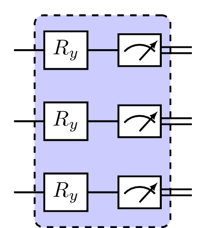
Figure 2: A three-qubit Ry measurement is simulated by $R_{y}$ gates operate on qubits followed by an ideal measurement.

For simplicity, we only apply Algorithm 1 to detect quantum noise of the first POVM element $E_{000}$. We remark that the same analysis is applicable to detect other POVM elements. Since the Ry measurement is composed of $R_{y}$ gates and an ideal measurement, its quantum noise measure can be analytically computed as

$$\mathscr{Q}_{\Phi}^{\theta}\left(E_{000}\right)=2\left|-0.018+0.236\cos(\theta)-0.018\cos(2\theta)\right|.$$ (26)

To collect experimental data, we uniformly sample $100$ $\theta$ values from $[0,2\pi]$. For each $\theta$, we estimate $\hat{\mathscr{Q}}_{\Phi}^{\theta}(E_{000})$ with a number of measurement shots $2^{13}$. Additionally, we repeat the estimation procedure $10^{3}$ times to report the average value and the standard deviation. Finally, we fit the estimated data to a Fourier series and obtain the fitting coefficients for $E_{000}$. The analytical, experimental, and fitted data are visualized in Figure 3. Notice that we have removed the absolute value restriction from the Figure for better illustration. One can see from the figure that the fitted Fourier series (red line) matches the theoretical curve (yellow line) pretty well, though there are statistical errors in the experimental data. That is to say, Algorithm 1 is robust to statistical error and reports the quantum noise measure $\mathscr{Q}_{\Phi}^{\theta}\left(E_{000}\right)$ with high accuracy, validating its practicability in detecting quantum noise of measurement devices.

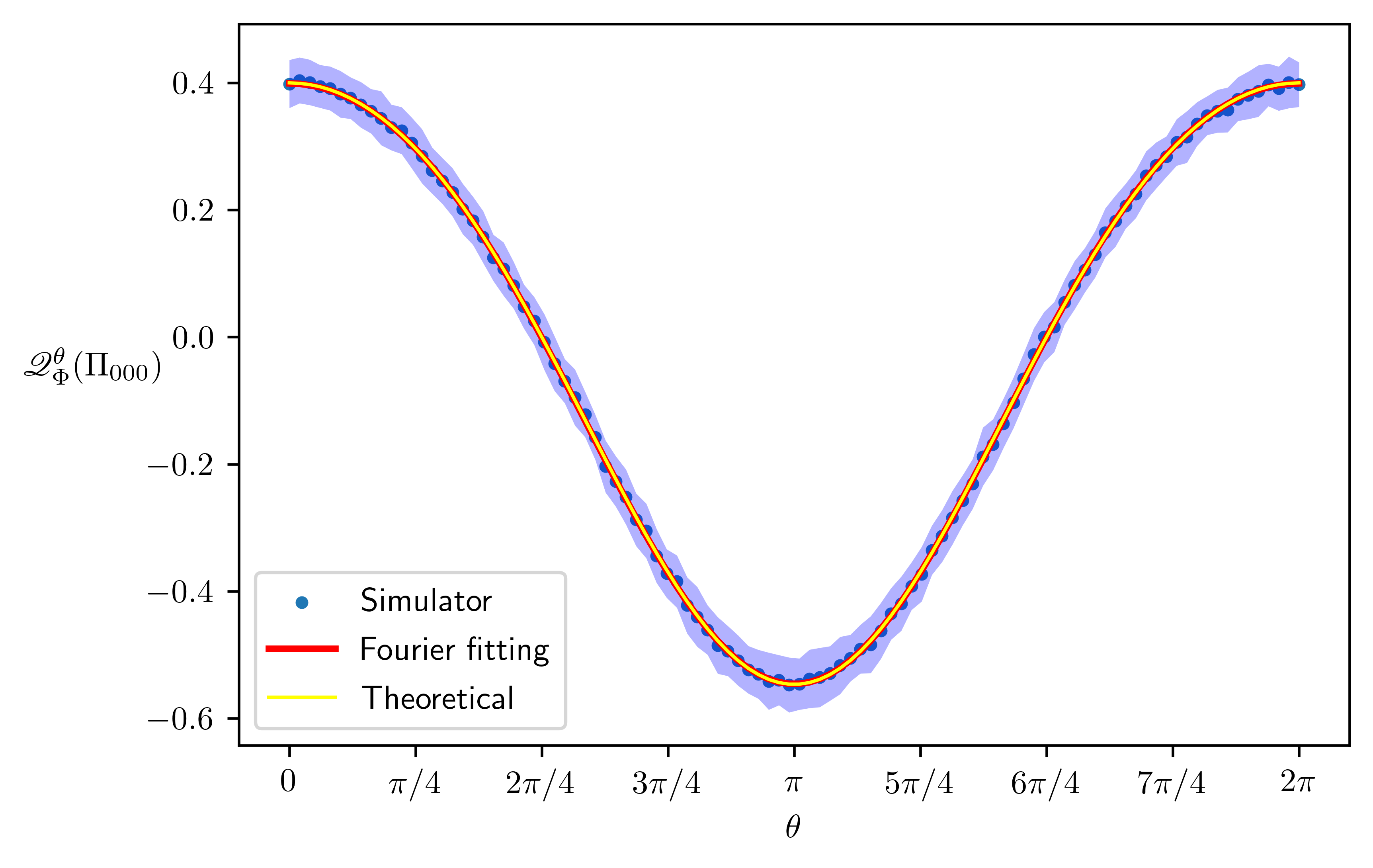
Figure 3: Detecting quantum noise in the simulated Ry measurement. We uniformly sample $100$ $\theta$ from $[0,2\pi]$. Experimental data on the Simulator are reported as the average value over $10^{3}$ independent estimations with standard error. Fourier fitting is plotted using the fitting coefficients obtained from the experimental data (cf. Algorithm 1). Theoretical is plotted using Eq. (26).

IV Quantum noise elimination

This section describes the second stage of the quantum noise manipulation process, introducing three techniques for quantum noise elimination. The effectiveness of these methods is evaluated on the Baidu Quantum Platform. They work by executing randomly sampled Pauli gates before the target measurement device and conditionally flipping the measurement outcomes in such a way that the effective measurement—composed of random Pauli gates, the noisy measurement device, and classical post-processing —contains only classical noise. These techniques are inspired by the established Pauli twirling approach [48, 49]. Notably, their fundamental distinction lies in the selection of the set of Pauli gates to be sampled.

Before presenting the technical details, we first briefly introduce the twirling technique. For any set $\mathbb{T}\subset\mathcal{U}(n)$, where $\mathcal{U}(n)$ denotes the set of $n$-qubit unitary matrices, we define the $\mathbb{T}$-twirl of a quantum channel $\mathcal{L}$ as

$$\mathcal{L}^{\mathbb{T}}\mathrel{\mathop{\mathchar 58\relax}}=\frac{1}{\left|\mathbb{T}\right|}\sum_{T\in\mathbb{T}}\mathcal{T}^{\dagger}\mathcal{L}\mathcal{T},$$ (27)

where $|\cdot|$ is the size of the set and $\mathcal{T}(\rho)\mathrel{\mathop{\mathchar 58\relax}}=T\rho T^{\dagger}$. Twirling involves the process of conjugating the noisy quantum channel $\mathcal{L}$ with a randomly selected gate $T$ from a predefined set of gates $\mathbb{T}$, termed the twirling set, each time a quantum circuit is executed. This technique holds significant importance in the field of quantum information theory. As an illustration, by choosing the twirling set to be the complete set of Pauli operators, we can convert any quantum channel into a Pauli channel whose noise elements correspond to the Pauli basis of the original noise [50, 51, 52, 53].

IV.1 IZ dephasing

Our first quantum noise elimination method is called the IZ dephasing. Interestingly, the idea of IZ dephasing comes from the observation that, in an estimating expectation value task, canceling the effect of the off-diagonal elements of the POVM elements is equivalent to canceling the impact of the off-diagonal parts of input quantum states. Now we formally elaborate on this observation.

The single-qubit completely dephasing channel $\Delta_{1}$ is defined as [41]

$$\Delta_{1}(\rho)\mathrel{\mathop{\mathchar 58\relax}}=\frac{1}{2}\rho+\frac{1}{2}Z\rho Z^{\dagger}=\begin{bmatrix}\rho_{0,0}&0\\ 0&\rho_{1,1}\end{bmatrix},$$ (28)

where $\rho_{i,j}$ is the element of $\rho$ in the $i$-th row and $j$-th column. Intuitively, $\Delta_{1}$ erases all off-diagonal terms (w.r.t. the computational basis) in $\rho$ while reserves the diagonal terms unchanged. The $n$-qubit completely dephasing channel is defined to be the $n$-th tensor product of $\Delta_{1}$:

$$\Delta_{n}(\rho)\mathrel{\mathop{\mathchar 58\relax}}=\Delta_{1}^{\otimes n}(\rho)=\sum_{\bm{x}}\left\langle{\bm{x}}\right|\rho\left|{\bm{x}}\right\rangle|{\bm{x}}\rangle\!\langle{\bm{x}}|.$$ (29)

Likewise, $\Delta_{n}$ erases all off-diagonal terms while reserving the diagonal terms unchanged.

For an arbitrary $n$-qubit quantum measurement channel $\mathcal{M}$, we define its $\Delta$-induced measurement channel as

$$\mathcal{M}^{\Delta}(\rho)\mathrel{\mathop{\mathchar 58\relax}}=\sum_{\bm{x}}\operatorname{Tr}[\Delta_{n}(E_{\bm{x}})\rho]|{\bm{x}}\rangle\!\langle{\bm{x}}|.$$ (30)

$\mathcal{M}^{\Delta}$ is constructed from $\mathcal{M}$ by erasing the off-diagonal elements of all POVM elements, via the completely dephasing channel $\Delta_{n}$. Notice that $\mathcal{M}^{\Delta}$ is indeed a measurement since $\Delta_{n}(E_{\bm{x}})\geq 0$ and

$$\sum_{\bm{x}}\Delta_{n}\left(E_{\bm{x}}\right)=\Delta_{n}\left(\sum_{\bm{x}}E_{\bm{x}}\right)=\Delta_{n}(\mathbbm{1})=\mathbbm{1},$$ (31)

where the last equality follows from the fact that $\Delta_{n}$ preserves the identity matrix. What’s more, $\mathcal{M}^{\Delta}$ is classical since all of its POVM elements have only diagonal elements. However, since neither $E_{\bm{x}}$ nor $\Delta_{n}(E_{\bm{x}})$ are legitimate quantum states, we are not able to realize the POVM elements $\Delta_{n}(E_{\bm{x}})$. Using the fact that the adjoint map of $\Delta_{n}$ is itself, i.e., $\Delta_{n}^{\dagger}=\Delta_{n}$, we have

$$\mathcal{M}^{\Delta}_{n}(\rho) =\sum_{\bm{x}}\operatorname{Tr}[\Delta_{n}(E_{\bm{x}})\rho]|{\bm{x}}\rangle\!\langle{\bm{x}}|$$ (32a)

$$=\sum_{\bm{x}}\operatorname{Tr}[E_{\bm{x}}\Delta_{n}^{\dagger}(\rho)]|{\bm{x}}\rangle\!\langle{\bm{x}}|$$ (32b)

$$=\sum_{\bm{x}}\operatorname{Tr}[E_{\bm{x}}\Delta_{n}(\rho)]|{\bm{x}}\rangle\!\langle{\bm{x}}|$$ (32c)

$$=\mathcal{M}(\Delta_{n}(\rho)).$$ (32d)

This equation mathematically justifies our observation and indicates that we can effectively implement the classical measurement $\mathcal{M}^{\Delta}$ from the original measurement $\mathcal{M}$ by completely dephasing the input quantum states first. The above result is rigorously summarized in the following theorem.

Theorem 6 (IZ dephasing).

Let $\mathcal{M}$ be a measurement channel in $\mathcal{H}_{n}$. The IZ-dephased linear map

$$\mathcal{M}^{\operatorname{IZ}}(\cdot)\mathrel{\mathop{\mathchar 58\relax}}=\mathcal{M}^{\Delta}(\cdot)=\frac{1}{2^{n}}\sum_{P\in\{I,Z\}^{\otimes n}}\mathcal{M}(P(\cdot)P),$$ (33)

is a classical measurement channel.

We show in Appendix F that the IZ dephasing method in Theorem 6 can be equivalently understood within the twirling framework (27) via

$$\mathcal{M}^{\operatorname{IZ}}(\cdot)=\frac{1}{2^{n}}\sum_{P\in\{I,Z\}^{\otimes n}}P\mathcal{M}(P(\cdot)P)P.$$ (34)

This alternative interpretation enables us to master all quantum noise elimination methods in a unified way within the twirling framework, as we will show.

Operationally, Theorem 6 motivates a simple experimental procedure to eliminate the quantum noise of measurement devices. Concretely, before sending the quantum states to the measurement device, we randomly sample a Pauli gate $P$ from the set $\operatorname{IZ}\equiv\{I,Z\}^{\otimes n}$ and operate it on the quantum states. Theorem 6 guarantees that the averaged output classical state after measurement would not be contaminated by quantum noise, though it still suffers from the classical noise of the measurement device. Extra elimination costs are incurred due to random sampling and averaging. The detailed procedure is summarized in Algorithm 2.

Algorithm 2 Quantum noise elimination via IZ dephasing

0:  $\bm{E}$: the $n$-qubit measurement device,      $\rho$: the input $n$-qubit quantum state,      $K$: number of $n$-qubit Pauli operators to be sampled,      $N_{\rm shots}$: number of measurement shots.

0:  $\hat{p}$, an estimate of $\operatorname{diag}(\rho)$ contaminated by classical noise.

1:  for $k=1,\cdots,K$ do

2:     Randomly sample a $n$-qubit Pauli gate $P_{k}\in\{I,Z\}^{\otimes n}$;

3:     Generate $N_{\rm shots}$ number of copies of the quantum state $\rho$ and apply the sampled Pauli gate $P_{k}$ to each of the quantum states;

4:     Perform the device $\bm{E}$ on the above quantum states and record the number of occurrences $N_{\bm{x}}^{(k)}$ of outcome $\bm{x}\in\{0,1\}^{n}$;

5:     Estimate an empirical probability distribution $\hat{p}^{(k)}$ via

$$\hat{p}^{(k)}_{\bm{x}}=N_{\bm{x}}^{(k)}/N_{\rm shots},\;\forall\bm{x}\in\{0,1\}^{n}.$$

6:  end for

7:  Calculate the mean value $\hat{p}$ from the estimated empirical probability distributions $\{\hat{p}^{(k)}\mathrel{\mathop{\mathchar 58\relax}}k=1,\cdots,K\}$ via

$$\hat{p}_{\bm{x}}=\frac{1}{K}\sum_{k=1}^{K}\hat{p}^{(k)}_{\bm{x}},\;\forall\bm{x}\in\{0,1\}^{n}.$$

Notice that $\hat{p}$ is an unbiased estimate of $\operatorname{diag}(\rho)$ contaminated only by classical noise of $\bm{E}$.

8:  Output $\hat{p}$.

IV.2 XY twirling

Our second quantum noise elimination method is called the XY twirling. This method is inspired by a careful inspection on the PTM representation of measurement channels. Specifically, we infer from Eq. (3) that, the PTM $[\mathcal{M}^{c}]$ of a classical measurement channel $\mathcal{M}^{c}$ has a desirable property that $[\mathcal{M}^{c}]_{\bm{i}\bm{j}}=0$ for arbitrary $P_{\bm{j}}\not\in\{I,Z\}^{\otimes n}$. That is to say, only matrix elements whose column indices corresponding to Pauli operators in the subset $\{I,Z\}^{\otimes n}$ have non-zero values. On the other hand, the PTM $[\mathcal{M}]$ of a general measurement channel $\mathcal{M}$ does not satisfy such property. There might exist some column index $\bm{j}$ such that $P_{\bm{j}}\not\in\left\{I,Z\right\}^{\otimes n}$ and $\left[\mathcal{M}\right]_{\bm{i}\bm{j}}\neq 0$. This observation yields an intuitive way to deal with quantum noise: If we can erase all those elements in the PTM matrix that are unique for quantum measurement, we obtain a new PTM matrix that corresponds to a classical measurement. Fortunately, we find that twirling an unknown measurement channel with the set $\operatorname{XY}=\{X,Y\}^{\otimes n}$ can erase all those unique elements and achieve our goal. We formally state this finding in the following theorem, and the proof is given in Appendix G.

Theorem 7 (XY twirling).

Let $\mathcal{M}$ be a measurement channel in $\mathcal{H}_{n}$. The XY-twirled linear map

$$\mathcal{M}^{\operatorname{XY}}(\cdot)\mathrel{\mathop{\mathchar 58\relax}}=\frac{1}{2^{n}}\sum_{P\in\{X,Y\}^{\otimes n}}P\mathcal{M}(P(\cdot)P)P$$ (35)

is a classical measurement channel.

Algorithm 3 Quantum noise elimination via XY twirling

0:  $\bm{E}$: the $n$-qubit measurement device,      $\rho$: the input $n$-qubit quantum state,      $K$: number of $n$-qubit Pauli operators to be sampled,      $N_{\rm shots}$: number of measurement shots.

0:  $\hat{p}$, an estimate of $\operatorname{diag}(\rho)$ contaminated by classical noise.

1:  for $k=1,\cdots,K$ do

2:     Randomly sample a $n$-qubit Pauli gate $P_{k}\in\{X,Y\}^{\otimes n}$;

3:     Generate $N_{\rm shots}$ number of copies of the quantum state $\rho$ and apply the sampled Pauli gate $P_{k}$ to each of the quantum states;

4:     Perform the device $\bm{E}$ on the above quantum states and record the number of occurrences $N_{\bm{x}}^{(k)}$ of outcome $\bm{x}\in\{0,1\}^{n}$;

5:     Estimate an empirical probability distribution $\hat{p}^{(k)}$ via

$$\hat{p}^{(k)}_{\bm{x}}=N_{\overline{\bm{x}}}^{(k)}/N_{\rm shots},\;\forall\bm{x}\in\{0,1\}^{n},$$

where $\overline{\bm{x}}$ is obtained from $\bm{x}$ by flipping all bits.

6:  end for

7:  Calculate the mean value $\hat{p}$ from the estimated empirical probability distributions $\{\hat{p}^{(k)}\mathrel{\mathop{\mathchar 58\relax}}k=1,\cdots,K\}$ via

$$\hat{p}_{\bm{x}}=\frac{1}{K}\sum_{k=1}^{K}\hat{p}^{(k)}_{\bm{x}},\;\forall\bm{x}\in\{0,1\}^{n}.$$

Notice that $\hat{p}$ is an unbiased estimate of $\operatorname{diag}(\rho)$ contaminated only by classical noise of $\bm{E}$.

8:  Output $\hat{p}$.

Much like Algorithm 2, Theorem 7 stimulates the following experimental procedure to eliminate the quantum noise of measurement devices. Specifically, before sending the quantum states to the measurement device, we randomly sample a Pauli gate $P$ from the twirling set $\operatorname{XY}\equiv\{X,Y\}^{\otimes n}$ and operate it on the quantum states. Then we measure the transformed states. After measurement, we have to operate the Pauli gate $P$ again on the classical output states to accomplish the twirling procedure, which is different from Algorithm 2. The tricky point is that since a measurement channel takes a quantum system to a classical one and the logical output states are classical, operating Pauli gates sampled from $\operatorname{XY}$ is equivalent to flipping the outcome bits, i.e., $0\to 1$ and $1\to 0$, which can be done through classical post-processing. Theorem 7 guarantees that the final averaged output classical state approximates the diagonal part of the input quantum state $\rho$, but is suffering from the classical noise of the measurement device. The detailed procedure is summarized in Algorithm 3.

IV.3 Pauli twirling

Our last quantum noise elimination method is the Pauli twirling. This method has the same spirit as the XY twirling method and aims to erase the elements in the PTM matrix that are unique for quantum measurement. Indeed, the idea of using Pauli twirling to eliminate quantum noise of measurement devices has been previously conceived in [49]. Here we present their proposal in a rigorous and experimental friendly way in the following proposition. The proof is given in Appendix H.

Proposition 8 (Pauli twirling).

Let $\mathcal{M}$ be a measurement channel in $\mathcal{H}_{n}$. The Pauli-twirled linear map

$$\mathcal{M}^{\operatorname{Pauli}}(\cdot)\mathrel{\mathop{\mathchar 58\relax}}=\frac{1}{4^{n}}\sum_{P\in\{I,X,Y,Z\}^{\otimes n}}P\mathcal{M}(P(\cdot)P)P$$ (36)

is a classical measurement channel.

Comparing Eqs. (33), (35), and (36), we can see that the Pauli twirling method has a much larger twirling set that incorporates the twirling sets of IZ dephasing and XY twirling. As before, Proposition 8 motivates a simple experimental procedure to eliminate the quantum noise of measurement devices. Concretely, before sending the quantum states to the measurement device, we randomly sample a Pauli gate $P$ from the set $\operatorname{Pauli}\equiv\{I,X,Y,Z\}^{\otimes n}$ and operate it on the quantum states. Then we measure the transformed states. After measurement, we have to operate the Pauli gate $P$ again on the output quantum states to accomplish the twirling procedure. Different from Algorithm 3, here we have to flip the outcome bits conditionally, since $I$ and $Z$ gates have different behavior to $X$ and $Y$ gates on the computational basis states. That is, we will flip the $n$-bit binary string $\bm{x}$ conditioned on the Pauli gate $P$: if the $i$-th operator of $P$ is $I$ or $Z$, we do not flip the $i$-th bit of $\bm{x}$; if the $i$-th operator of $P$ is $X$ or $Y$, we flip the $i$-th bit of $\bm{x}$. Proposition 8 guarantees that the averaged output approximates the diagonal part of the input quantum state $\rho$, which only suffers from the classical noise of the measurement device. The detailed procedure is summarized in Algorithm 4.

Algorithm 4 Quantum noise elimination via Pauli twirling

0:  $\bm{E}$: the $n$-qubit measurement device,      $\rho$: the input $n$-qubit quantum state,      $K$: number of $n$-qubit Pauli operators to be sampled,      $N_{\rm shots}$: number of measurement shots.

0:  $\hat{p}$, an estimate of $\operatorname{diag}(\rho)$ contaminated by classical noise.

1:  for $k=1,\cdots,K$ do

2:     Randomly sample a $n$-qubit Pauli gate $P_{k}\in\{I,X,Y,Z\}^{\otimes n}$;

3:     Generate $N_{\rm shots}$ number of copies of the quantum state $\rho$ and apply the sampled Pauli gate $P_{k}$ to each of the quantum states;

4:     Perform the device $\bm{E}$ on the above quantum states and record the number of occurrences $N_{\bm{x}}^{(k)}$ of outcome $\bm{x}\in\{0,1\}^{n}$;

5:     Estimate an empirical probability distribution $\hat{p}^{(k)}$ via

$$\hat{p}^{(k)}_{\bm{x}}=N_{\overline{\bm{x}}}^{(k)}/N_{\rm shots},\;\forall\bm{x}\in\{0,1\}^{n},$$

where $\overline{\bm{x}}$ is obtained from $\bm{x}$ by conditionally flipping the bits based on the Pauli operator $P_{k}$: If the $i$-th operator of $P_{k}$ is $X$ or $Y$, then flip the $i$-th bit of $\bm{x}$; otherwise, do not flip.

6:  end for

7:  Calculate the mean value $\hat{p}$ from the estimated empirical probability distributions $\{\hat{p}^{(k)}\mathrel{\mathop{\mathchar 58\relax}}k=1,\cdots,K\}$ via

$$\hat{p}_{\bm{x}}=\frac{1}{K}\sum_{k=1}^{K}\hat{p}^{(k)}_{\bm{x}},\;\forall\bm{x}\in\{0,1\}^{n}.$$

Notice that $\hat{p}$ is an unbiased estimate of $\operatorname{diag}(\rho)$ contaminated only by classical noise of $\bm{E}$.

8:  Output $\hat{p}$.

IV.4 Comparisons

We have proposed three methods to eliminate quantum noise in measurement devices. Here we discuss the similarities, advantages, and differences among these methods.

First, we note that all these methods can be described in a unified way within the twirling framework. Following the compiling idea of [49], these methods can be experimentally implemented with only classical pre-and post-processing, without truly inserting the sampled Pauli gates before the measurement device. More precisely, we can compile the sampled Pauli gate with the last gates in the quantum circuit that generates the quantum state, optimizing two quantum gates into one. This compiling requires only a tiny classical overhead in the compilation cost and can be implemented on the fly with fast classical control.

The IZ dephasing method utilizes a twirling set of size $2^{n}$ and does not require bits to flip after measurement. Besides, since we do not need to insert ‘I’ gates in practice, the number of quantum gates inserted is $n2^{n-1}$. What’s more, from Eq. (32) we can see that this method removes off-diagonal values but preserves diagonal values of the POVM elements. That is, we do not change the classical behavior of the measurement device. The XY twirling method utilizes a twirling set of size $2^{n}$ but requires bits to flip after measurement, which incurs extra classical possessing cost. The total number of quantum gates inserted is $n2^{n}$, twice of the former method. Moreover, it removes not only off-diagonal values but also changes diagonal values of the POVM elements, causing unpredictable classical behavior. The Pauli twirling method is the most expensive since it utilizes a twirling set of size $4^{n}$ and requires a conditional flip after measurement. The total number of quantum gates inserted is $n4^{n}$, much larger than the former methods. It removes not only off-diagonal values but also regularizes diagonal values of POVM elements, so that the diagonal values of different POVM elements are the same but reordered.

Notice that some methods not only erase the off-diagonal values but also change the diagonal values of original POVM elements. We are interested in whether they will dramatically alter the fidelity of the measurement device, which is essential since if these methods result in substantial decay in the fidelity, we have to scarify fidelity for quantum noise. Luckily, we can show that the measurement fidelity is robust to these methods in the sense that it remains unchanged by these methods. Before presenting the main result, let’s first define the measurement fidelity. The measurement fidelity, also known as readout fidelity and assignment fidelity, of a quantum measurement $\mathcal{M}$ (with respect to the computational basis measurement) is defined as [54]

$$f(\mathcal{M})\mathrel{\mathop{\mathchar 58\relax}}=\frac{1}{2^{n}}\sum_{\bm{x}\in\{0,1\}^{n}}\langle\bm{x}|E_{\bm{x}}|\bm{x}\rangle.$$ (37)

Intuitively, $f(\mathcal{M})$ quantifies how well $\mathcal{M}$ preserves the computational basis states on average. Then, we have the following identification among the measurement fidelities of the effective measurements. The proof is given in Appendix I.

Proposition 9.

Let $\mathcal{M}$ be a measurement channel in $\mathcal{H}_{n}$. It holds that

$$f(\mathcal{M})=f(\mathcal{M}^{\operatorname{IZ}})=f(\mathcal{M}^{\operatorname{XY}})=f(\mathcal{M}^{\operatorname{Pauli}}).$$ (38)

Proposition 9 implies that although Pauli twirling employs many more Pauli gates to eliminate quantum noise, it cannot make the resulting effective measurement channel in the sense of measurement fidelity. One thus wonders if the Pauli twirling technique could bring any advantage. Indeed, we show that Pauli twirling can simplify the classical noise process by regularizing the POVM elements, as formally stated in the following proposition. The proof is given in Appendix J.

Proposition 10.

Let $\mathcal{M}$ be a measurement channel in $\mathcal{H}_{n}$ and $\mathcal{M}^{\operatorname{Pauli}}$ be its Pauli-twirled channel. It holds that

$$\operatorname{diag}(E_{\bm{y}}^{\operatorname{Pauli}})=\mathsf{T}_{\bm{y}}\mathsf{T}_{\bm{x}}^{-1}\operatorname{diag}(E_{\bm{x}}^{\operatorname{Pauli}}),$$ (39)

where the transition matrix $\mathsf{T}_{{\bm{x}}}$ is defined as

$$\left(\mathsf{T}_{{\bm{x}}}\right)_{\bm{i}\bm{j}}\mathrel{\mathop{\mathchar 58\relax}}=(-1)[({\bm{x}}+\bm{i})\cdot\bm{j}].$$ (40)

where $\bm{a}\cdot\bm{b}$ is the bitwise inner product between $\bm{a}$ and $\bm{b}$ and

$$(-1)[\bm{a}]\mathrel{\mathop{\mathchar 58\relax}}=\prod_{\bm{a}_{i}\in\bm{a}}(-1)^{\bm{a}_{i}}.$$ (41)

Proposition 10 implies that there exist strong correlations among the POVM elements of the Pauli-twirled measurement channel: they share the same diagonal values, and their order is specified by the outcome label $\bm{x}$. Thus, given the knowledge of an arbitrary POVM element, we can completely infer the remaining POVM elements via Eq. (39). This lovely property can be employed in quantum detector tomography as a constraint to improve the estimation accuracy of Pauli-twirled measurement channels.

V Experimental results

In this section, we test the two-stage procedure with three quantum applications—estimating the expectation value of Mermin polynomial, the fidelity of GHZ states, and the ground state energy of a hydrogen molecule—using a noisy simulator with Ry measurements (cf. Figure 3) on Baidu Quantum Platform, to showcase its ability in improving computation accuracy. The experimental data are collected via the QCompute Software Development Kit [40]. All experiments were performed with $N_{\rm{shots}}=2^{13}$ number of shots.

V.1 Expectation value of Mermin polynomial

	Unmitigated	Inverse	Least square	IBU
Raw	$10.775\pm 0.033$	$11.335\pm 0.035$	$11.340\pm 0.035$	$11.335\pm 0.035$
IZ dephasing	$10.768\pm 0.008$	$11.313\pm 0.008$	$11.318\pm 0.008$	$11.313\pm 0.008$
XY twirling	$10.766\pm 0.008$	$11.315\pm 0.009$	$11.320\pm 0.009$	$11.315\pm 0.009$
Pauli twirling	$10.767\pm 0.002$	$11.315\pm 0.002$	$11.320\pm 0.003$	$11.315\pm 0.002$

Table 1: The four-qubit Mermin polynomial (V.1) measured on Baidu Quantum Platform. The theoretical maximum value allowed by quantum mechanics is $8\sqrt{2}\approx 11.314$. Experimental data are reported as the average value over $10^{3}$ independent estimations with standard error. The Raw, IZ dephasing, XY twirling, and Pauli twirling rows record the values without or with the corresponding quantum noise elimination methods. The Unmitigated, Inverse, Least square, and IBU columns record the values without or with the corresponding error mitigation methods.

Our first application is to estimate the expectation values of Mermin polynomials [55], which are one of the most significant examples to test non-local quantum correlations in multi-partite systems. We notice that many research groups have measured Mermin polynomials on superconducting quantum computers to assess their quantum reliability [56, 57, 58, 59, 60, 24]. We measure the following $4$-qubit Mermin polynomial

$$M_{4} \mathrel{\mathop{\mathchar 58\relax}}=\left\langle XXXY\right\rangle+\left\langle XXYX\right\rangle+\left\langle XYXX\right\rangle+\left\langle YXXX\right\rangle$$

$$+\left\langle XXYY\right\rangle+\left\langle XYXY\right\rangle+\left\langle XYYX\right\rangle+\left\langle YXXY\right\rangle$$

$$+\left\langle YXYX\right\rangle+\left\langle YYXX\right\rangle-\left\langle XXXX\right\rangle-\left\langle XYYY\right\rangle$$

$$-\left\langle YXYY\right\rangle-\left\langle YYXY\right\rangle-\left\langle YYYX\right\rangle+\left\langle YYYY\right\rangle$$ (42)

on the quantum state

$$\left|{G}\right\rangle\mathrel{\mathop{\mathchar 58\relax}}=\frac{|0000\rangle+e^{3\pi i/4}|1111\rangle}{\sqrt{2}}.$$ (43)

Note that the state $\left|{G}\right\rangle$ can be prepared by the quantum circuit described in [24, Fig. 1(b)]. We choose this state because it allows for a maximal violation of local realism. Experimentally, the Mermin polynomial (V.1) is measured on the first four qubits of the simulator after preparing the quantum state (43). We use the proposed elimination methods to cancel the effect of quantum noise. Besides, we adopt four error mitigation methods—the inverse method (Inverse) [28], the least square method (Least square) [25], and the iterative Bayesian unfolding method (IBU) [27]—to reverse the classical noise effect and improve the estimation accuracy. Note that we use the implementations of these mitigation methods in Baidu Quantum Platform .

The experimental results are summarized in Table 1. We find from the second column that the effects of both classical and quantum noises are significant, as reflected in the differences between the raw and theoretical values. Moreover, though the elimination methods alone cannot improve the estimation accuracy, they considerably decrease the statistical error, making the estimation procedure more robust. We find that the second row error mitigation methods in the presence of quantum noise would lead to an overestimation of the entanglement, indicating that it should not be trusted in quantum foundations experiments like this. We also find from the remaining rows that the difference in the estimated values between the three elimination methods is statistically insignificant and is insensitive to different error mitigation techniques. In other words, all these methods can accurately eliminate quantum noise in the measurement device. This justifies our expectation that the two-stage procedure and error mitigation techniques form a standard toolbox for manipulating measurement errors.

V.2 Fidelity of GHZ states

Our second application is to estimate the fidelity of multi-partite GHZ states via parity oscillation, which is a standard method for checking the entanglement of GHZ states [62]. The parity oscillation protocol works as follows: first, we generate a $n$-qubit GHZ state using Hadamard and CNOT gates; then, we apply the same rotation operation $U_{\phi}=e^{\mathrm{i}\pi\sigma_{\phi}/4}$ to all qubits of the GHZ state, where $\sigma_{\phi}\mathrel{\mathop{\mathchar 58\relax}}=\cos{\phi}X+\sin{\phi}Y$; finally, we measure the qubits on the computational basis and estimate the expectation value of observable $Z^{\otimes n}$. By varying the phase $\phi$, we can observe an oscillation effect of the expectation values and the oscillation intensity benchmarks the prepared GHZ state’s entanglement quality. Experimentally, we consider a $4$-qubit system, where the GHZ state has the form

$$\left|{\operatorname{GHZ}}\right\rangle\mathrel{\mathop{\mathchar 58\relax}}=\frac{\left|{0000}\right\rangle+\left|{1111}\right\rangle}{\sqrt{2}}.$$ (44)

We prepare this state on the first four qubits $\{Q_{0},Q_{1},Q_{2},Q_{3}\}$ of the noisy simulator. As in the case of the Mermin polynomial, we use the elimination methods to cancel the effect of quantum noise and adopt the least square method to mitigate the impact of classical noise.

The experimental results are summarized in Figure 4. We tell from the significant gap between the raw data (with and without error mitigation) and theoretical curves that the effect of quantum noise is quite significant. We also tell from the minor gaps between the eliminated and theoretical curves that all three elimination methods collaborate pretty well with the least square mitigation method. They together remarkably improve the computation accuracy. What’s more, we conclude from the minor estimation errors there is no statistical difference among these elimination methods.

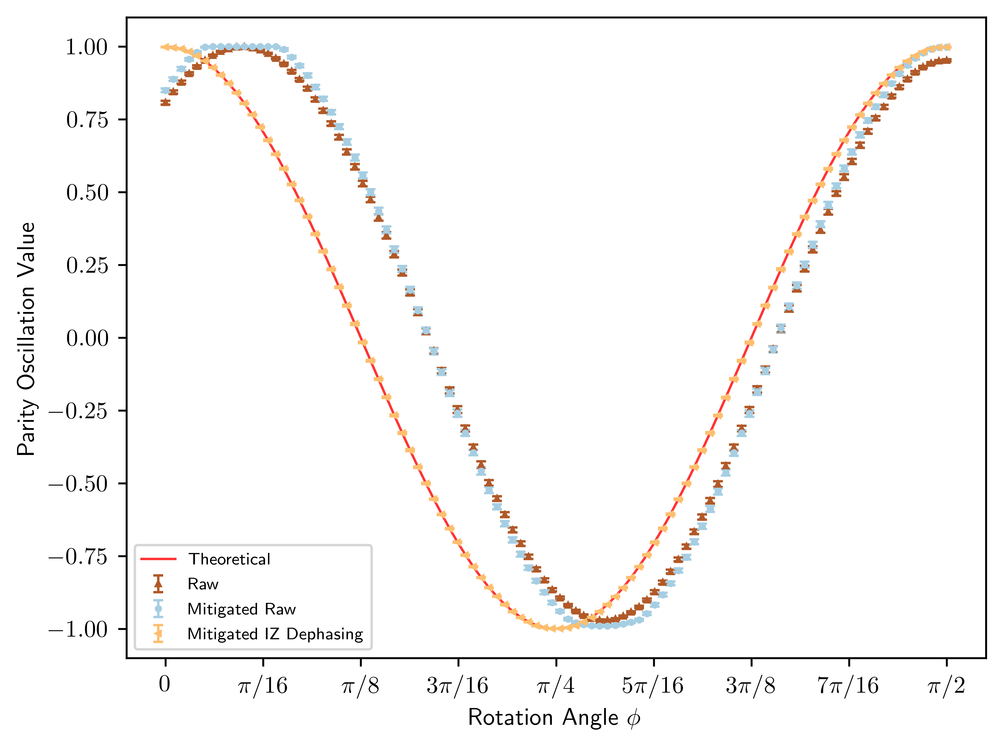
Figure 4: Parity oscillation of the four-qubit GHZ state (44) measured on Baidu Quantum Platform. Experimental data are reported as the average value over $10^{2}$ independent estimations with standard error. Theoretical values (red line) are analytically calculated. Raw (brown upper triangle) and Mitigated Raw (blue circle) are collected without or with the least square error mitigation. Mitigated IZ dephasing (yellow left triangle) values are collected by first eliminating quantum noise using the corresponding method and then performing least square error mitigation.

V.3 Ground state energy of hydrogen molecule

Our last application is to estimate the ground state energy of hydrogen molecules by running the flagship algorithm Variational Quantum Eigensolver (VQE) [63] on the noisy simulator. Briefly speaking, the inputs to a VQE algorithm are a Hamiltonian $H$ of the hydrogen molecule and a parametrized circuit that prepares a trial state $\left|{\psi(\bm{\theta})}\right\rangle$ aiming to approximate the ground state of the molecule. Within VQE, the cost function is defined to be the expectation value of the Hamiltonian computed in the trial state $f(\bm{\theta})\mathrel{\mathop{\mathchar 58\relax}}=\left\langle{\psi(\bm{\theta})}\right|H\left|{\psi(\bm{\theta})}\right\rangle$, which can be estimated by measuring $\psi(\bm{\theta})$. The ground state of the target Hamiltonian is obtained by performing an iterative cost function minimization. The optimization is carried out by a classical optimizer which leverages a quantum computer to evaluate the cost function and calculate its gradient at each optimization step. The $4$-qubit Hamiltonian of hydrogen molecule we apply is obtained from the OpenFermion library [64] and the exact form is given in Appendix K. We construct a $4$-qubit variational ansatz $\left|{\psi(\bm{\theta})}\right\rangle$ consisting of an initial state $\left|{0}\right\rangle^{\otimes 4}$ followed by $6$ repetitions of a layer of parameterized single-qubit $Y$-rotations on each qubit and a layer of CZ gates between alternating qubits. The parameters $\bm{\theta}$ are randomly initialized and the classical optimizer is chosen as the sequential minimal optimization (SMO) method.

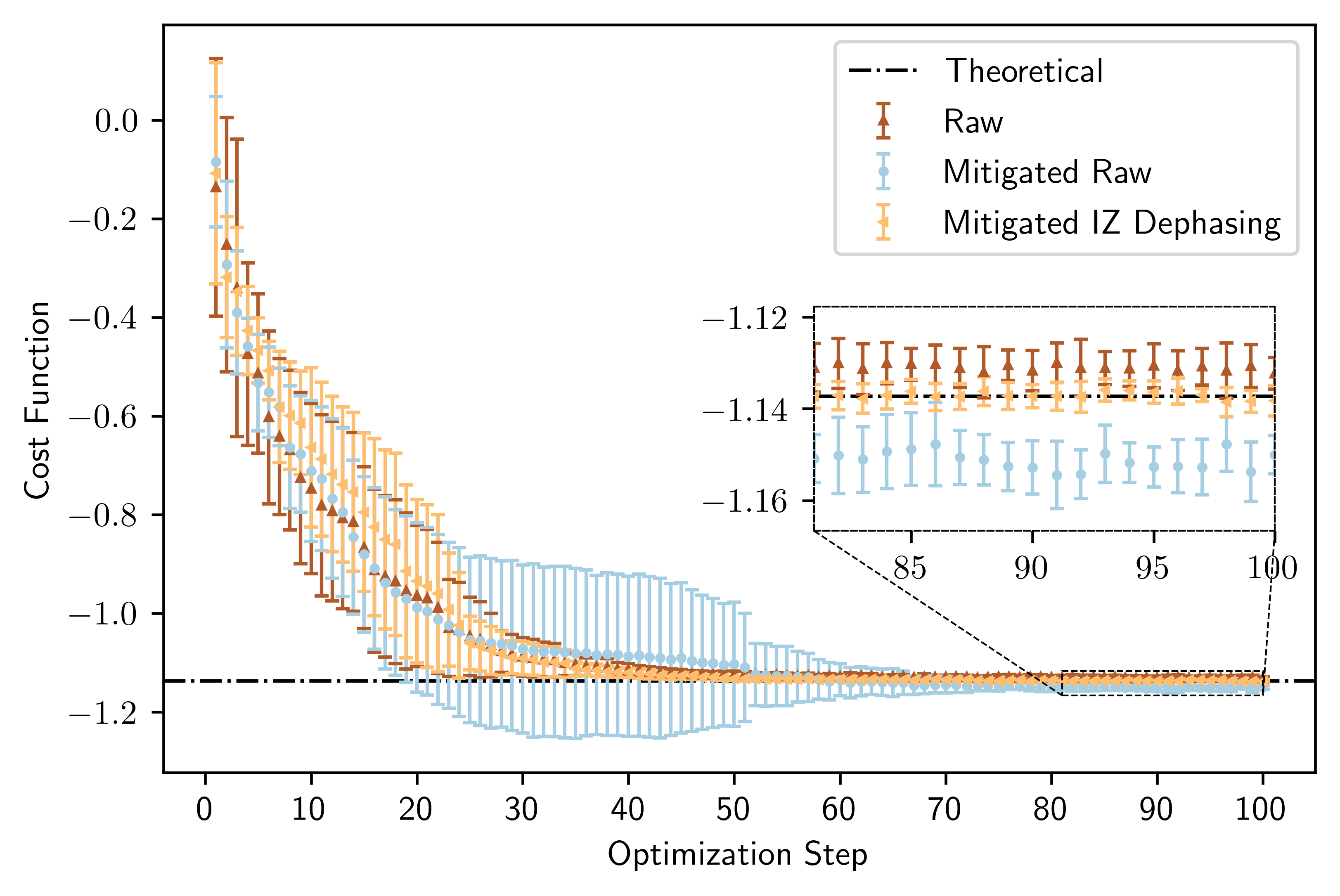
Figure 5: The ground state energy of hydrogen molecule measured on Baidu Quantum Platform. Experimental data are reported as the average value over $10$ independent estimations with standard error. Theoretical (black dashed line) gives the theoretical ground energy $-1.137$. Raw (brown upper triangle) and Mitigated Raw (blue circle) values are collected without or with the least square error mitigation. Mitigated IZ dephasing (yellow left triangle) values are collected by first eliminating quantum noise with IZ dephasing and then performing least square error mitigation.

The experimental results are summarized in Figure 5. We need to point out that we did not use the XY and Pauli twirling methods because they achieve the same performance as the IZ dephasing method as revealed in previous applications. The Mitigated IZ dephasing data shows that quantum noise elimination combined with error mitigation can greatly improve the effectiveness of VQE algorithms, yields an accurate estimation of the ground stat energy. On the other hand, we prove in Appendix K that the Raw data actually estimates the ground state energy of a transformed Hamiltonian whose theoretical value should be $-1.135$. The data matches this theoretical value pretty well. When we execute the error mitigation method in the presence of quantum noise, we see from Mitigated Raw that we obtain an overestimation ($-1.152$) of the ground state energy. This indicates that we should be cautious when performing measurement error mitigation methods: if the measurement contains quantum noise, mitigation would be harmful instead of useful.

We find from the slow convergence rate of the raw cost function that VQE is immensely sensitive to measurement noise. In the absence of noise elimination, the noisy cost function deviates significantly from its noiseless counterpart, which can greatly limit the effectiveness of VQE algorithms, even for a small number of qubits. We also find that the eliminated and mitigated cost values converge much faster and are slightly more accurate than raw ones.

VI Conclusions

The main contribution of this work is a two-stage procedure that systematically addresses quantum noise inherent in NISQ measurement devices. The procedure is incredibly intuitive: we first detect and then eliminate quantum noise if there is any. In the first stage, we prepared maximally coherent states $\left|{\Phi_{\theta}}\right\rangle$ with relative phase $\theta$ and maximally mixed states as inputs to the measurement device and fitted the difference between two measurement statistics to the Fourier series. The fitting coefficients quantitatively benchmark the quantum noise of the measurement device. In the second stage, we executed randomly sampled Pauli gates before the measurement device. We conditionally flipped the outcomes so that the resulting effective measurement contains only classical noise. We demonstrated the procedure’s practicability numerically on Baidu Quantum Platform, via two paradigmatic quantum applications. Remarkably, these results revealed that quantum noise in the measurement devices under investigation are significantly suppressed, and the computation accuracy of the applications is substantially improved. This two-stage procedure complements existing measurement error mitigation techniques, and we believe that they together form a standard toolbox for manipulating measurement errors in near-term quantum devices.

We have seen the devastating impact of quantum noise when mitigating measurement noises. This motivates us to study quantum noise from a resource theoretic perspective, possibly termed a resource theory of decoherence, which may revolutionize how we understand and manipulate noises inherent in quantum measurement devices. Also, it is worth discovering if there are more efficient ways to eliminate quantum noise other than the methods inspired by Pauli twirling.

Acknowledgements. S. T. and C. Z. contributed equally to this work. This work was done when S. T. and C. Z. were research interns at Baidu Research. We would like to thank Runyao Duan for helpful discussions.

Appendix A Alternative definition of quantum noise witness

Let’s consider the following alternative definition of quantum noise witness, where the separation hyperplane is determined by the expectation values less than or equal to $0$.

Definition 2’.

Let $W$ be a Hermitian operator in $\mathcal{H}_{n}$. $W$ is called a quantum noise witness, if

1. for arbitrary classical POVM $\{E^{c}_{\bm{x}}\}_{\bm{x}}$, it holds for arbitrary $\bm{x}$ that $\operatorname{Tr}[WE^{c}_{\bm{x}}]\leq 0$;

2. there exists at least one quantum POVM $\{E^{q}_{\bm{x}}\}_{\bm{x}}$ such that there exists some $\bm{x}$ for which $\operatorname{Tr}[WE^{q}_{\bm{x}}]>0$.

Thus, if one measures $\operatorname{Tr}[WE_{\bm{x}}]<0$ for some $E_{\bm{x}}$, one knows for sure that this POVM element, and the corresponding POVM, contains quantum noise.

Let $W$ be a quantum noise witness defined w.r.t. Definition 2’ and let $\mathcal{S}$ be the set of quantum POVM elements that can be detected by $W$, i.e.,

$$\forall E_{\bm{x}}^{q}\in\mathcal{S},\operatorname{Tr}[WE_{\bm{x}}^{q}]>0.$$ (45)

We will construct a quantum noise witness $\widetilde{W}$ from $W$ satisfying the following two conditions: 1) for arbitrary classical POVM element $E^{c}_{\bm{x}}$, $\operatorname{Tr}[\widetilde{W}E^{c}_{\bm{x}}]=0$; and 2) $\forall E_{\bm{x}}^{q}\in\mathcal{S}$, $\operatorname{Tr}[\widetilde{W}E_{\bm{x}}^{q}]\neq 0$. That is to say, given arbitrary witness defined w.r.t. Definition 2’, we can always construct a new witness which satisfies Definition 2 in the main text and the quantum POVM elements that can be detected by the former can also be detected by the latter. Since a witness defined w.r.t. Definition 2 naturally satisfies Definition 2’, we conclude that these two definitions are equivalent.

The construction is as follows. Define the following operator

$$\widetilde{W}\mathrel{\mathop{\mathchar 58\relax}}=W-D_{W},$$ (46)

where $D_{W}$ is the diagonal part of $W$. Note that $\widetilde{W}$ is Hermitian whenever $W$ is. By definition it is easy to see that $\widetilde{W}$ only has non-zero off-diagonal elements. For an arbitrary classical POVM element $E_{\bm{x}}^{c}$, it holds that

$$\operatorname{Tr}[\widetilde{W}E_{\bm{x}}^{c}]=\operatorname{Tr}[WE_{\bm{x}}^{c}]-\operatorname{Tr}[D_{W}E_{\bm{x}}^{c}]=0,$$ (47)

since $E_{\bm{x}}^{c}$ only has non-zero diagonal elements. On the other hand, for arbitrary quantum POVM element $E_{\bm{x}}^{q}\in\mathcal{S}$, it holds that

$$\operatorname{Tr}[\widetilde{W}E_{x}^{q}]=\operatorname{Tr}[WE_{x}^{q}]-\operatorname{Tr}[D_{W}E_{x}^{q}]=\operatorname{Tr}[WE_{x}^{q}]-\operatorname{Tr}[WD_{E_{x}^{q}}],$$ (48)

where $D_{E_{x}^{q}}$ is the diagonal part of $E_{x}^{q}$. Notice that $\operatorname{Tr}[WE_{x}^{q}]>0$ since $E_{\bm{x}}^{q}\in\mathcal{S}$ and $\operatorname{Tr}[WD_{E_{x}^{q}}]\leq 0$ since $D_{E_{x}^{q}}$ is a classical POVM and $W$ is defined w.r.t. Definition 2’. Therefore, $\operatorname{Tr}[\widetilde{W}E_{x}^{q}]\neq 0$.

Appendix B Proof of Proposition 3

Assume the spectral decomposition $W_{\psi}=\sum_{i}\lambda_{i}|{i}\rangle\!\langle{i}|$, where $W_{\psi}$ is a quantum noise witness defined in (8) and $\{\left|{i}\right\rangle\}_{i}$ forms an orthonormal basis. For arbitrary probe state $\psi$, the density matrix can be written as $\rho=|{\psi}\rangle\!\langle{\psi}|$. Assume $\left|{\psi}\right\rangle=\sum_{i}\alpha_{i}\left|{i}\right\rangle$, and

$$W_{\psi} =\frac{\mathbbm{1}}{2^{n}}-|{\psi}\rangle\!\langle{\psi}|=\frac{\mathbbm{1}}{2^{n}}-\sum_{i,j}\alpha_{i}\alpha_{j}|{i}\rangle\!\langle{j}|.$$ (49)

Therefore,

$$\operatorname{Tr}[W_{\psi}E_{\bm{x}}^{q}] =\operatorname{Tr}[\frac{\mathbbm{1}}{2^{n}}D_{E_{\bm{x}}^{q}}]-\sum_{i,j}\alpha_{i}\alpha_{j}\left\langle{j}\right|E_{\bm{x}}^{q}\left|{i}\right\rangle$$ (50)

$$=\sum_{i}\left(\frac{1}{2^{n}}-|{\alpha_{i}}|^{2}\right)\left\langle{i}\right|E_{\bm{x}}^{q}\left|{i}\right\rangle-\sum_{i\neq j}\alpha_{i}\alpha_{j}\left\langle{j}\right|E_{\bm{x}}^{q}\left|{i}\right\rangle.$$ (51)

As long as $|{\alpha_{i}}|^{2}=\frac{1}{2^{n}}$, Eq. (51) would give $-\sum_{i\neq j}\alpha_{i}\alpha_{j}\left\langle{j}\right|E_{\bm{x}}^{q}\left|{i}\right\rangle$. When $\operatorname{Tr}[W_{\psi}E_{\bm{x}}^{q}]\neq 0$, we can always say that there exists quantum noise.

Appendix C Properties of quantum noise measure

In this section, we explore general properties, analytical solutions in the qubit case, and the relations to the resource theory of quantum measurements of the $\psi$-induced quantum noise measure $\mathscr{Q}_{\psi}$ in Definition 4 of the main text.

C.1 General properties

First of all, we show that for arbitrary POVM element $E_{\bm{x}}$, the quantity $\mathscr{Q}_{\psi}(E_{\bm{x}})$ is normalized.

Lemma 11 (Normalization).

Let $E_{\bm{x}}$ be an arbitrary POVM element. It holds that $\mathscr{Q}_{\psi}(E_{\bm{x}})\in\left[0,1\right]$.

Proof.

First we show that for arbitrary positive semidefinite matrix $A$ it holds that

$$|A_{i,j}|\leq\sqrt{A_{i,i}A_{j,j}},$$ (52)

where $A_{i,j}$ is the element in the $i$-th row and $j$-th column. For a positive semidefinite matrix $A$, all of its principal submatrices are positive semidefinite. Furthermore, $\operatorname{Tr}{A}$, $\det{A}$ as well as the principal minors of $A$ are all nonnegative [65]. Consider the following $2\times 2$ principal minor

$$\widehat{A}\mathrel{\mathop{\mathchar 58\relax}}=\begin{bmatrix}A_{i,i}&A_{i,j}\\ A_{i,j}^{\dagger}&A_{jj}\end{bmatrix}.$$ (53)

It holds that

$$\det(\widehat{A})=A_{i,i}A_{j,j}-|A_{i,j}|^{2}\geq 0,$$ (54)

which leads to (52).

For arbitrary POVM element $E_{\bm{x}}$, since it is positive semidefinite, we obtain from Eq. (52) that

$$|E_{\bm{x}}(\bm{y},\bm{z})|\leq\sqrt{E_{\bm{x}}(\bm{y},\bm{y})E_{\bm{x}}(\bm{z},\bm{z})}.$$ (55)

Therefore,

$$\left|\sum_{\bm{y}\neq\bm{z}}E_{\bm{x}}(\bm{y},\bm{z})\right|\leq\sum_{\bm{y}\neq\bm{z}}\left|E_{\bm{x}}(\bm{y},\bm{z})\right|\leq\sum_{\bm{y}\neq\bm{z}}\sqrt{E_{\bm{x}}(\bm{y},\bm{y})E_{\bm{x}}(\bm{z},\bm{z})}.$$ (56)

On the other hand, since $\sum_{\bm{x}}E_{\bm{x}}=I$ and $E_{\bm{x}}\geq 0$, it follows that $0\leq E_{\bm{x}}(\bm{y},\bm{y})\leq 1$ for all $\bm{y}$. Thus

$$\sqrt{E_{\bm{x}}(\bm{y},\bm{y})E_{\bm{x}}(\bm{z},\bm{z})}\leq\sum_{\bm{y}\neq\bm{z}}\sqrt{E_{\bm{x}}(\bm{y},\bm{y})E_{\bm{x}}(\bm{z},\bm{z})}\leq\sum_{\bm{y}\neq\bm{z}}E_{\bm{x}}(\bm{y},\bm{y})E_{\bm{x}}(\bm{z},\bm{z})\leq\sum_{\bm{y}}E_{\bm{x}}(\bm{y},\bm{y})=1.$$ (57)

Finally, given

$$0\leq|e^{i(\theta_{\bm{z}}-\theta_{\bm{y}})}|\leq 1,$$ (58)

it’s obvious that

$$\mathscr{Q}_{\psi}(E_{\bm{x}})=|\sum_{\bm{y}\neq\bm{z}}e^{i(\theta_{\bm{z}}-\theta_{\bm{y}})}E_{\bm{x}}(\bm{y},\bm{z})|\leq 1.$$ (59)

∎

Lemma 12 (Additivity).

Let $\bm{E}^{(1)}=\{E^{(1)}_{\bm{x}}\}_{\bm{x}\in\{0,1\}^{n}}$ and $\bm{E}^{(2)}=\{E^{(2)}_{\bm{x}}\}_{\bm{x}\in\{0,1\}^{n}}$ be two POVMs. For arbitrary $\bm{x}\in\{0,1\}^{n}$, it holds that

$$\mathscr{Q}_{\psi}(E_{\bm{x}}^{(1)}\otimes E_{\bm{x}}^{(2)})\leq 2(\mathscr{Q}_{\psi}(E_{\bm{x}}^{(1)})+\mathscr{Q}_{\psi}(E_{\bm{x}}^{(2)})).$$ (60)

Correspondingly,

$$\mathscr{Q}_{\psi}(\bm{E}^{(1)}\otimes\bm{E}^{(2)})\leq 2(\mathscr{Q}_{\psi}(\bm{E}^{(1)})+\mathscr{Q}_{\psi}(\bm{E}^{(2)})).$$ (61)

Proof.

Consider $2$ qubits case. Assume that for qubit $0$ and qubit $1$,

$$E_{0}^{(0)}=\left[\begin{matrix}a_{0}&\gamma_{0}\\ \gamma_{0}^{\ast}&b_{0}\end{matrix}\right],\quad\quad E_{1}^{(0)}=\left[\begin{matrix}1-a_{0}&-\gamma_{0}\\ -\gamma_{0}^{\ast}&1-b_{0}\end{matrix}\right],$$ (62)

$$E_{0}^{(1)}=\left[\begin{matrix}a_{1}&\gamma_{1}\\ \gamma_{1}^{\ast}&b_{1}\end{matrix}\right],\quad\quad E_{1}^{(1)}=\left[\begin{matrix}1-a_{1}&-\gamma_{1}\\ -\gamma_{1}^{\ast}&1-b_{1}\end{matrix}\right].$$ (63)

We can see that

$$\mathscr{Q}_{\Phi}(E^{(0)}_{0})+\mathscr{Q}_{\Phi}(E^{(1)}_{0})=2\left|\Re(\gamma_{0})\right|+2\left|\Re(\gamma_{1})\right|.$$ (64)

Then,

$$E_{00}=E_{0}^{(0)}\otimes E_{1}^{(1)}=\left[\begin{matrix}a_{0}E_{0}^{(1)}&\gamma_{0}E_{0}^{(1)}\\ \gamma_{0}^{\ast}E_{0}^{(1)}&b_{0}E_{0}^{(1)}\end{matrix}\right].$$ (65)

Expand Eq. (65) we get

$$E_{00}=\left[\begin{matrix}a_{0}a_{1}&a_{0}\gamma_{1}&\gamma_{0}a_{1}&\gamma_{0}\gamma_{1}\\ a_{0}\gamma^{\ast}_{1}&a_{0}b_{1}&\gamma_{0}\gamma_{1}^{\ast}&\gamma_{0}b_{1}\\ \gamma_{0}^{\ast}a_{1}&\gamma_{0}^{\ast}\gamma_{1}&b_{0}a_{1}&b_{0}\gamma_{1}\\ \gamma_{0}^{\ast}\gamma_{1}^{\ast}&\gamma_{0}^{\ast}b_{1}&b_{0}\gamma_{1}^{\ast}&b_{0}b_{1}\end{matrix}\right].$$ (66)

Then

$$\mathscr{Q}_{\Phi}(E_{00})=2\left|(a_{0}+b_{0})\Re(\gamma_{1})+(a_{1}+b_{1})\Re(\gamma_{0})+2\Re(\gamma_{0})\Re(\gamma_{1})\right|.$$ (67)

Let’s consider the maximum case. Assume $a_{0}=a_{1}=1$, $b_{0}=b_{1}=1$. Eq. (67) turns into

$$\max(\mathscr{Q}_{\Phi}(E_{00})) =4\left|\Re(\gamma_{1})+\Re(\gamma_{0})+\Re(\gamma_{0}\gamma_{1})+\Re(\gamma_{0}\gamma_{1}^{\ast})\right|$$ (68)

$$=4\left|\Re(\gamma_{1})+\Re(\gamma_{0})+2\Re(\gamma_{0})\Re(\gamma_{1})\right|.$$ (69)

Through triangle inequality,

$$\left|\Re(\gamma_{1})+\Re(\gamma_{0})+2\Re(\gamma_{0})\Re(\gamma_{1})\right| \leq\left|\Re(\gamma_{1})+\Re(\gamma_{0})|+|2\Re(\gamma_{0})\Re(\gamma_{1})\right|$$ (70)

$$\leq\left|\Re(\gamma_{1})+\Re(\gamma_{0})\right|$$ (71)

$$\leq\left|\Re(\gamma_{1})\right|+\left|\Re(\gamma_{0})\right|.$$ (72)

Therefore,

$$\max(\mathscr{Q}_{\Phi}(E_{00}))\leq 2(\mathscr{Q}_{\Phi}(E^{(0)}_{0})+\mathscr{Q}_{\Phi}(E^{(1)}_{0})).$$ (73)

Without loss of generality, we can conclude that

$$\mathscr{Q}_{\psi}(E_{\bm{x}}^{(1)}\otimes E_{\bm{x}}^{(2)})\leq 2(\mathscr{Q}_{\psi}(E_{\bm{x}}^{(1)})+\mathscr{Q}_{\psi}(E_{\bm{x}}^{(2)})).$$ (74)

Correspondingly,

$$\mathscr{Q}_{\psi}(\bm{E}^{(1)}\otimes\bm{E}^{(2)})\leq 2(\mathscr{Q}_{\psi}(\bm{E}^{(1)})+\mathscr{Q}_{\psi}(\bm{E}^{(2)})).$$ (75)

∎

Lemma 13 (Convexity).

Let $\bm{E}^{(1)}=\{E^{(1)}_{\bm{x}}\}_{\bm{x}\in\{0,1\}^{n}}$ and $\bm{E}^{(2)}=\{E^{(2)}_{\bm{x}}\}_{\bm{x}\in\{0,1\}^{n}}$ be two POVMs. For arbitrary $p\in[0,1]$ and $\bm{x}\in\{0,1\}^{n}$, it holds that

$$\mathscr{Q}_{\psi}(pE_{\bm{x}}^{(1)}+(1-p)E_{\bm{x}}^{(2)})\leq p\mathscr{Q}_{\psi}(E_{\bm{x}}^{(1)})+(1-p)\mathscr{Q}_{\psi}(E_{\bm{x}}^{(2)}).$$ (76)

Correspondingly,

$$\mathscr{Q}_{\psi}(p\bm{E}^{(1)}+(1-p)\bm{E}^{(2)})\leq p\mathscr{Q}_{\psi}(\bm{E}^{(1)})+(1-p)\mathscr{Q}_{\psi}(\bm{E}^{(2)}).$$ (77)

Proof.

For arbitrary $p\in[0,1]$, we have

$$\mathscr{Q}(pE_{\bm{x}}^{(1)}+(1-p)E_{\bm{x}}^{(2)}) =2^{n}\left|\operatorname{Tr}[W_{\psi}(pE_{\bm{x}}^{(1)}+(1-p)pE_{\bm{x}}^{(2)})]\right|$$ (78)

$$=2^{n}\left|\operatorname{Tr}[pW_{\psi}E_{\bm{x}}^{(1)}]+\operatorname{Tr}[(1-p)W_{\psi}E_{\bm{x}}^{(2)}]\right|$$ (79)

$$=2^{n}\left|p\operatorname{Tr}[W_{\psi}E_{\bm{x}}^{(1)}]+(1-p)\operatorname{Tr}[W_{\psi}E_{\bm{x}}^{(2)}]\right|$$ (80)

and

$$p\mathscr{Q}(E_{\bm{x}}^{(1)})+(1-p)\mathscr{Q}(E_{\bm{x}}^{(2)})=2^{n}\left|p\operatorname{Tr}[W_{\psi}E_{\bm{x}}^{(1)}]\right|+2^{n}\left|(1-p)\operatorname{Tr}[W_{\psi}E_{\bm{x}}^{(2)}]\right|.$$ (81)

From triangle inequality,

$$\left|p\operatorname{Tr}[W_{\psi}E_{\bm{x}}^{(1)}]+(1-p)\operatorname{Tr}[W_{\psi}E_{\bm{x}}^{(2)}]\right|\leq\left|p\operatorname{Tr}[W_{\psi}E_{\bm{x}}^{(1)}]\right|+\left|(1-p)\operatorname{Tr}[W_{\psi}E_{\bm{x}}^{(2)}]\right|.$$ (82)

Therefore,

$$\mathscr{Q}(pE_{\bm{x}}^{(1)}+(1-p)E_{\bm{x}}^{(2)})\leq p\mathscr{Q}(E_{\bm{x}}^{(1)})+(1-p)\mathscr{Q}(E_{\bm{x}}^{(2)}).$$ (83)

∎

C.2 Single and two-qubit case

Let’s begin with the single-qubit case. Consider a qubit POVM $\{E_{0},E_{1}\}$ with

$$E_{0}=\begin{bmatrix}\alpha&a_{1}+ib_{1}\\ a_{1}-ib_{1}&\beta\\ \end{bmatrix},\qquad E_{1}=\begin{bmatrix}1-\alpha&-a_{1}-ib_{1}\\ -a_{1}+ib_{1}&1-\beta\end{bmatrix},$$ (84)

where $\alpha,\beta,a_{1},b_{1}\in\mathbb{R}$. We have

$$\mathscr{Q}^{\theta}_{\Phi}(E_{0})=2\left|-a_{1}\cos(\theta)+b_{1}\sin(\theta)\right|,\qquad\mathscr{Q}^{\theta}_{\Phi}(E_{1})=2\left|a_{1}\cos(\theta)-b_{1}\sin(\theta)\right|.$$ (85)

It is obvious that we just need to consider $2$ special cases in order to extract the absolute values of $a_{1}$ and $b_{1}$. Specifically,

$$\mathscr{Q}^{\theta=0}_{\Phi}(E_{0}) =\mathscr{Q}^{\theta=0}_{\Phi}(E_{1})=2\left|a_{1}\right|,$$ (86)

$$\mathscr{Q}^{\theta=\pi/2}_{\Phi}(E_{0}) =\mathscr{Q}^{\theta=\pi/2}_{\Phi}(E_{1})=2\left|b_{1}\right|.$$ (87)

Now we consider the two-qubit case. The density matrix of two-qubit $\Phi_{\theta}$ (12) has the form

$$\Phi_{\theta}=\frac{1}{4}\left[\begin{array}[]{cccc}1&e^{-i\theta}&e^{-i\theta}&e^{-i2\theta}\\ e^{i\theta}&1&1&e^{-i\theta}\\ e^{i\theta}&1&1&e^{-i\theta}\\ e^{i2\theta}&e^{i\theta}&e^{i\theta}&1\end{array}\right].$$ (92)

Suppose we have an unknown POVM element $E$ parameterized as

$$E=\left[\begin{array}[]{cccc}a_{11}&a_{12}&a_{13}&a_{14}\\ a_{12}^{\ast}&a_{22}&a_{23}&a_{24}\\ a_{13}^{\ast}&a_{23}^{\ast}&a_{33}&a_{34}\\ a_{14}^{\ast}&a_{24}^{\ast}&a_{34}^{\ast}&a_{44}\end{array}\right].$$ (97)

After some tedious calculation we obtain

$$\mathscr{Q}_{\Phi}^{\theta}(E) =2\left|-\cos{(\theta)}\Re({a_{12}+a_{13}+a_{24}+a_{34}})+\sin{(\theta)}\Im{(a_{12}+a_{13}+a_{24}+a_{34}})\right.$$

$$\left.\quad\quad-\cos{(2\theta)}\Re{(a_{14})}+\sin{(2\theta)}\Im{(a_{14})}-\Re{(a_{23})}\right|$$ (98)

$$=2\left|-a_{0}-a_{1}\cos{(\theta)}-a_{2}\cos{(2\theta)}+b_{1}\sin{(\theta)}+b_{2}\sin{(2\theta)}\right|,$$ (99)

where

$$a_{0} =\Re{(a_{23})},$$ (100)

$$a_{1} =\Re({a_{12}+a_{13}+a_{24}+a_{34}}),$$ (101)

$$a_{2} =\Re{(a_{14})},$$ (102)

$$b_{1} =\Im{(a_{12}+a_{13}+a_{24}+a_{34}}),$$ (103)

$$b_{2} =\Im{(a_{14})}.$$ (104)

C.3 Relation to quantum resource theory

In [47], the authors formalized a resource theoretical framework to quantify the coherence of quantum measurements and introduced a coherence monotone of measurement in terms of off-diagonal values of the POVM elements. Specifically, Let $\bm{E}=\{E_{\bm{x}}\}_{\bm{x}}$ be a POVM, the $\ell_{\infty}$-coherence monotone of $\bm{E}$ is defined as [47, Eq. (10)]

$$\mathcal{C}_{\ell_{\infty}}(\bm{E})\mathrel{\mathop{\mathchar 58\relax}}=\sum_{\bm{x}}\sum_{\bm{y}<\bm{z}}\left|E_{\bm{x}}(\bm{y},\bm{z})\right|.$$ (105)

We can show that the quantum noise measure $\mathscr{Q}_{\Phi}$ bounds the $\ell_{\infty}$-coherence monotone from below. This result, together with Theorem 1 in [47], establishes an experimental-friendly lower bound on the critical quantum measurement robustness measure originally introduced in [47].

Lemma 14.

Let $\bm{E}=\{E_{\bm{x}}\}_{\bm{x}}$ be a POVM in $\mathcal{H}_{n}$. It holds that

$$\mathcal{C}_{\ell_{\infty}}(\bm{E})\geq 2^{n-1}\mathscr{Q}_{\Phi}^{\theta=0}(\bm{E}).$$ (106)

Proof.

By definition (11), we have

$$\mathscr{Q}_{\Phi}^{\theta=0}(\bm{E}) =\frac{1}{2^{n}}\sum_{\bm{x}}\mathscr{Q}_{\Phi}^{\theta=0}(E_{\bm{x}})$$ (107)

$$=\frac{1}{2^{n-1}}\sum_{\bm{x}}\left|\sum_{\bm{y}<\bm{z}}E_{\bm{x}}(\bm{y},\bm{z})\right|$$ (108)

$$\leq\frac{1}{2^{n-1}}\sum_{\bm{x}}\sum_{\bm{y}<\bm{z}}\left|E_{\bm{x}}(\bm{y},\bm{z})\right|$$ (109)

$$=\frac{1}{2^{n-1}}\mathcal{C}_{\ell_{\infty}}(\bm{E}),$$ (110)

leading to (106). ∎

Appendix D Proof of Theorem 5

Notice that the prob state $\Phi_{\theta}$ defined in (12) of the main text can be equivalently expressed as

$$\left|{\Phi_{\theta}}\right\rangle=\frac{1}{\sqrt{2^{n}}}\sum_{\bm{y}}e^{i\theta\left|\bm{y}\right|}\left|{\bm{y}}\right\rangle,$$ (111)

where $|\bm{y}|$ represents the Hamming weight of the binary string $\bm{y}$. Thus

$$\Phi_{\theta}\equiv|{\Phi_{\theta}}\rangle\!\langle{\Phi_{\theta}}|=\frac{1}{2^{n}}\sum_{\bm{y,z}}e^{i\theta(\left|\bm{y}\right|-\left|\bm{z}\right|)}|{\bm{y}}\rangle\!\langle{\bm{z}}|.$$ (112)

According to Eq. (9), it holds that

$$\mathscr{Q}_{\Phi}^{\theta}(E_{\bm{x}}) =2^{n}\left|\operatorname{Tr}[W_{\Phi}E_{\bm{x}}]\right|$$ (113)

$$=2^{n}\left|\operatorname{Tr}\left[\left(\frac{1}{2^{n}}\mathbbm{1}-\Phi_{\theta}\right)E_{\bm{x}}\right]\right|$$ (114)

$$=\left|\operatorname{Tr}\left[\left(\mathbbm{1}-\sum_{\bm{y,z}}e^{i\theta(\left|\bm{y}\right|-\left|\bm{z}\right|)}|{\bm{y}}\rangle\!\langle{\bm{z}}|\right)E_{\bm{x}}\right]\right|$$ (115)

$$=\left|\sum_{\bm{y}\neq\bm{z}}\operatorname{Tr}[(-e^{i\theta(\left|\bm{y}\right|-\left|\bm{z}\right|)}|{\bm{y}}\rangle\!\langle{\bm{z}}|)E_{\bm{x}}]\right|$$ (116)

$$=\left|-\sum_{\bm{y}\neq\bm{z}}e^{i\theta(\left|\bm{y}\right|-\left|\bm{z}\right|)}E_{\bm{x}}(\bm{y},\bm{z})\right|$$ (117)

$$=2\left|-\sum_{\bm{y<z}}\Re\left[E_{\bm{x}}(\bm{y},\bm{z})\right]\cos\left[\left(\left|\bm{y}\right|-\left|\bm{z}\right|\right)\theta\right]+\Im\left[E_{\bm{x}}(\bm{y},\bm{z})\right]\sin\left[\left(\left|\bm{y}\right|-\left|\bm{z}\right|\right)\theta\right]\right|,$$ (118)

where Eq. (118) follows from the conjugated property of the off-diagonal values of a POVM element.

It is worth pointing out that $\bm{y}<\bm{z}$ does not implies $\left|\bm{y}\right|<\left|\bm{z}\right|$ in general. For example, when $\bm{y}=011$ and $\bm{z}=100$, we can see that $\bm{y}<\bm{z}$ and $\left|\bm{y}\right|=2>\left|\bm{z}\right|=1$.

Appendix E Proof of Proposition 1

First of all, we introduce some notations concerning the Pauli operators. The Pauli group $\mathsf{P}^{n}=\left\{I,X,Y,Z\right\}^{\otimes n}$ is Abelian and isomorphic to $\mathsf{Z}^{2n}_{2}$, where $\bm{a}\in\mathsf{Z}^{2n}_{2}$ is a $2n$ length binary string. Since $P_{\bm{a}}\in\mathsf{P}^{n}$ can be represented as

$$P_{\bm{a}}=P_{(\bm{a}_{x},\bm{a}_{z})}=i^{\bm{a}_{x}\cdot\bm{a}_{z}}X[\bm{a}_{x}]Z[\bm{a}_{z}],$$ (119)

where $\bm{a}_{x},\bm{a}_{z}\in\mathsf{Z}^{n}_{2}$ and $A[\bm{a}]\mathrel{\mathop{\mathchar 58\relax}}=\bigotimes_{\bm{a}_{i}\in\bm{a}}A^{\bm{a}_{i}}$. Given two Pauli operators $P_{\bm{a}}$ and $P_{\bm{b}}$, we have $P_{\bm{a}}P_{\bm{b}}=(-1)^{\langle\bm{a},\bm{b}\rangle}P_{\bm{b}}P_{\bm{a}}$ where

$$\langle\bm{a},\bm{b}\rangle=\bm{a}_{x}\cdot\bm{b}_{z}+\bm{a}_{z}\cdot\bm{b}_{x}.$$ (120)

In the following proof, we use rescaled Pauli operators $P_{\bm{a}}\to P_{\bm{a}}/\sqrt{2^{n}}$ so that the basis is properly normalized.

Now let’s prove Proposition 1. Notice that the PTM $[\mathcal{M}]$ of a measurement channel $\mathcal{M}$ satisfies

$$[\mathcal{M}]_{\bm{i}\bm{j}} =\operatorname{Tr}[P_{\bm{i}}\mathcal{M}(P_{\bm{j}})]=\sum_{\bm{x}}\operatorname{Tr}[E_{\bm{x}}P_{\bm{j}}]\langle\bm{x}|P_{\bm{i}}|\bm{x}\rangle=\begin{cases}\sum_{\bm{x}}\operatorname{Tr}[E_{\bm{x}}P_{\bm{j}}]\langle\bm{x}|P_{\bm{i}}|\bm{x}\rangle,&P_{\bm{i}}\in\{I,Z\}^{\otimes n}\\ 0,&P_{\bm{i}}\not\in\{I,Z\}^{\otimes n}\end{cases}.$$ (121)

From this equation, we can see that an element of $[\mathcal{M}]$ is non-zero if and only if its row index corresponds to Pauli operators in the subset $\{I,Z\}^{\otimes n}$.

We express Eq. (121) in matrix form as

$$[\mathcal{M}]=[\mathsf{P}][E],$$ (122)

where $[\mathsf{P}]_{\bm{i}\bm{x}}\mathrel{\mathop{\mathchar 58\relax}}=\langle\bm{x}|P_{\bm{i}}|\bm{x}\rangle$ and $[E]_{\bm{x}\bm{j}}\mathrel{\mathop{\mathchar 58\relax}}=\operatorname{Tr}[E_{\bm{x}}P_{\bm{j}}]$. Notice that

$$[\mathsf{P}]^{\dagger}[\mathsf{P}] =\left(\sum_{\bm{j},\bm{y}}\langle\bm{y}|P_{\bm{j}}|\bm{y}\rangle|{\bm{y}}\rangle\!\langle{\bm{j}}|\right)\left(\sum_{\bm{i},\bm{x}}\langle\bm{x}|P_{\bm{i}}|\bm{x}\rangle|{\bm{i}}\rangle\!\langle{\bm{x}}|\right)$$ (123)

$$=\sum_{\bm{i},\bm{x},\bm{y}}\langle\bm{x}|P_{\bm{i}}|\bm{x}\rangle\langle\bm{y}|P_{\bm{i}}|\bm{y}\rangle|{\bm{y}}\rangle\!\langle{\bm{x}}|$$ (124)

$$=\sum_{\bm{x},\bm{y}}|{\bm{y}}\rangle\!\langle{\bm{x}}|\sum_{\bm{i}}\langle\bm{x}|P_{\bm{i}}|\bm{x}\rangle\langle\bm{y}|P_{\bm{i}}|\bm{y}\rangle$$ (125)

$$=\sum_{\bm{x},\bm{y}}|{\bm{y}}\rangle\!\langle{\bm{x}}|\left(\sum_{\bm{i}}\langle\bm{x}|Z[\bm{i}_{z}]|\bm{x}\rangle\langle\bm{y}|Z[\bm{i}_{z}]|\bm{y}\rangle\right)$$ (126)

$$=\sum_{\bm{x},\bm{y}}|{\bm{y}}\rangle\!\langle{\bm{x}}|\left(\frac{1}{2^{n}}\sum_{\bm{i}}(-1)\left[\bm{i}_{z}\cdot\bm{x}\right](-1)\left[\bm{i}_{z}\cdot\bm{y}\right]\right)$$ (127)

$$=\sum_{\bm{x},\bm{y}}|{\bm{y}}\rangle\!\langle{\bm{x}}|\left(\frac{1}{2^{n}}\sum_{\bm{i}}(-1)\left[\bm{i}_{z}\cdot(\bm{x}+\bm{y})\right]\right)$$ (128)

$$=\sum_{\bm{x},\bm{y}}\delta_{\bm{x},\bm{y}}|{\bm{y}}\rangle\!\langle{\bm{x}}|$$ (129)

$$=\mathbbm{1},$$ (130)

we obtain from Eq. (122) that

$$[E]=[\mathsf{P}]^{\dagger}[\mathsf{P}][E]=[\mathsf{P}]^{\dagger}[\mathcal{M}].$$ (131)

This gives that for arbitrary $\bm{x}\in\{0,1\}^{n}$,

$$E_{\bm{x}}=\sum_{P_{\bm{j}}\in\mathsf{P}^{n}}[E]_{\bm{x}\bm{j}}P_{\bm{j}}=\sum_{P_{\bm{i}},P_{\bm{j}}\in\mathsf{P}^{n}}[\mathsf{P}]_{\bm{i}\bm{x}}[\mathcal{M}]_{\bm{i}\bm{j}}P_{\bm{j}}.$$ (132)

Appendix F Proof of Eq. (34)

Denote the RHS. of Eq. (34) as

$$\widetilde{\mathcal{M}}(\cdot)\mathrel{\mathop{\mathchar 58\relax}}=\frac{1}{2^{n}}\sum_{P\in\{I,Z\}^{\otimes n}}P\mathcal{M}(P(\cdot)P)P.$$ (133)

We need to show that for arbitrary $\rho$ it holds that

$$\mathcal{M}^{\operatorname{IZ}}(\rho)=\widetilde{\mathcal{M}}(\rho).$$ (134)

Consider the following chain of equalities:

$$\widetilde{\mathcal{M}}(\rho) =\frac{1}{2^{n}}\sum_{P\in\{I,Z\}^{\otimes n}}P\mathcal{M}(P\rho P)P$$ (135)

$$=\frac{1}{2^{n}}\sum_{P\in\{I,Z\}^{\otimes n}}P\left(\sum_{\bm{x}\in\Sigma}\operatorname{Tr}\left[E_{\bm{x}}P\rho P\right]|{\bm{x}}\rangle\!\langle{\bm{x}}|\right)P$$ (136)

$$=\frac{1}{2^{n}}\sum_{P\in\{I,Z\}^{\otimes n}}\sum_{\bm{x}\in\Sigma}\operatorname{Tr}\left[E_{\bm{x}}P\rho P\right]P|{\bm{x}}\rangle\!\langle{\bm{x}}|P$$ (137)

$$=\frac{1}{2^{n}}\sum_{P\in\{I,Z\}^{\otimes n}}\sum_{\bm{x}\in\Sigma}\operatorname{Tr}\left[E_{\bm{x}}P\rho P\right]|{\bm{x}}\rangle\!\langle{\bm{x}}|$$ (138)

$$=\mathcal{M}^{\operatorname{IZ}}(\rho),$$ (139)

where Eq. (136) follows from the definition of $\mathcal{M}$ in (2) and Eq. (138) follows from the fact that for arbitrary $P\in\{I,X\}$, $P|{0}\rangle\!\langle{0}|P=|{0}\rangle\!\langle{0}|$ and $P|{1}\rangle\!\langle{1}|P=|{1}\rangle\!\langle{1}|$, i.e., $P\in\{I,Z\}^{\otimes n}$ preserves the classical state $|{\bm{x}}\rangle\!\langle{\bm{x}}|$. We are done.

Appendix G Proof of Theorem 7

The PTM matrix of the XY-twirled measurement channel $\mathcal{M}^{\operatorname{XY}}$ has the form

$$[\mathcal{M}^{\operatorname{XY}}]_{\bm{i}\bm{j}} =\operatorname{Tr}\left[P_{\bm{i}}\mathcal{M}^{\operatorname{XY}}(P_{\bm{j}})\right]$$ (140)

$$=\frac{1}{2^{n}}\sum_{P_{\bm{k}}\in\{X,Y\}^{\otimes n}}\operatorname{Tr}\left[P_{\bm{i}}P_{\bm{k}}\mathcal{M}(P_{\bm{k}}P_{\bm{j}}P_{\bm{k}})P_{\bm{k}}\right]$$ (141)

$$=\left(\frac{1}{2^{n}}\sum_{P_{\bm{k}}\in\{X,Y\}^{\otimes n}}(-1)^{\langle\bm{i}+\bm{j},\bm{k}\rangle}\right)[\mathcal{M}]_{\bm{i}\bm{j}},$$ (142)

Note that

$$\frac{1}{2^{n}}\sum_{P_{\bm{k}}\in\{X,Y\}^{\otimes n}}(-1)^{\langle\bm{i}+\bm{j},\bm{k}\rangle}=\frac{1}{2^{n}}\sum_{P_{\bm{k}}\in\{X,Y\}^{\otimes n}}(-1)^{(\bm{i}+\bm{j})_{x}\cdot\bm{k}_{z}+(\bm{i}+\bm{j})_{z}\cdot\bm{k}_{x}}=\frac{(-1)^{(\bm{i}+\bm{j})_{z}}}{2^{n}}\sum_{P_{\bm{k}}\in\{X,Y\}^{\otimes n}}(-1)^{(\bm{i}+\bm{j})_{x}\cdot\bm{k}_{z}}.$$ (143)

Since we have shown in (121) that an element of $[\mathcal{M}]$ is non-zero if and only if its row index corresponds to Pauli operators in the subset $\{I,Z\}^{\otimes n}$, we can assume $P_{\bm{i}}\in\{I,Z\}^{\otimes n}$. Now let’s consider two cases of $P_{\bm{j}}$. If $P_{\bm{j}}\in\{I,Z\}^{\otimes n}$, it holds that

$$\frac{1}{2^{n}}\sum_{P_{\bm{k}}\in\{X,Y\}^{\otimes n}}(-1)^{(\bm{i}+\bm{j})_{x}\cdot\bm{k}_{z}}=1.$$ (144)

If $P_{\bm{j}}\not\in\{I,Z\}^{\otimes n}$, it holds that

$$\frac{1}{2^{n}}\sum_{P_{\bm{k}}\in\{X,Y\}^{\otimes n}}(-1)^{(\bm{i}+\bm{j})_{x}\cdot\bm{k}_{z}}=\frac{1}{2^{n}}\sum_{P_{k}\in\{X,Y\}^{\otimes n}}(-1)^{\bm{j}_{x}\cdot\bm{k}_{z}}=0.$$ (145)

Substituting Eqs. (144) and (145) into (142), we obtain

$$[\mathcal{M}^{\operatorname{XY}}]_{\bm{i}\bm{j}}=\begin{cases}(-1)^{(\bm{i}+\bm{j})_{z}}[\mathcal{M}]_{\bm{i}\bm{j}},&P_{\bm{j}}\in\{I,Z\}^{n},\\ 0&P_{\bm{j}}\not\in\{I,Z\}^{n}.\end{cases}$$ (146)

The POVM representation $\{E_{\bm{x}}^{\operatorname{XY}}\}_{\bm{x}}$ of $\mathcal{M}^{\operatorname{XY}}$ can be computed from its PTM matrix using Proposition 1 as

$$E_{\bm{x}}^{\operatorname{XY}}=\sum_{P_{\bm{i}},P_{\bm{j}}\in\mathsf{P}^{n}}[\mathsf{P}]_{\bm{i}\bm{x}}[\mathcal{M}^{\operatorname{XY}}]_{\bm{i}\bm{j}}P_{\bm{j}}=\sum_{P_{\bm{i}},P_{\bm{j}}\in\{I,Z\}^{\otimes n}}(-1)^{(\bm{i}+\bm{j})_{z}}[\mathsf{P}]_{\bm{i}\bm{x}}[\mathcal{M}]_{\bm{i}\bm{j}}P_{\bm{j}}.$$ (147)

For arbitrary $\bm{y}\neq\bm{z}$, it holds that

$$\left\langle{\bm{y}}\right|E_{\bm{x}}^{\operatorname{XY}}\left|{\bm{z}}\right\rangle=\sum_{P_{\bm{i}},P_{\bm{j}}\in\{I,Z\}^{\otimes n}}(-1)^{(\bm{i}+\bm{j})_{z}}[\mathsf{P}]_{\bm{i}\bm{x}}[\mathcal{M}]_{\bm{i}\bm{j}}\left\langle{\bm{y}}\right|P_{\bm{j}}\left|{\bm{z}}\right\rangle=0,$$ (148)

indicating that the POVM elements after XY twirling have zero non-diagonal elements.

Appendix H Proof of Proposition 8

From Eq. (142), we know that the PTM matrix of the Pauli-twirled measurement channel $\mathcal{M}^{\operatorname{Pauli}}$ has the form

$$[\mathcal{M}^{\operatorname{Pauli}}]_{\bm{i}\bm{j}}=\operatorname{Tr}\left[P_{\bm{i}}\mathcal{M}^{\operatorname{Pauli}}(P_{\bm{j}})\right]=\left(\frac{1}{2^{n}}\sum_{P_{\bm{k}}\in\{I,X,Y,Z\}^{\otimes n}}(-1)^{\langle\bm{i}+\bm{j},\bm{k}\rangle}\right)[\mathcal{M}]_{\bm{i}\bm{j}}.$$ (149)

Following a similar argument as that in Appendix G, we conclude that

$$[\mathcal{M}^{\operatorname{Pauli}}]_{\bm{i}\bm{j}}=\begin{cases}[\mathcal{M}]_{\bm{i}\bm{j}},&P_{\bm{i}}=P_{\bm{j}}\in\{I,Z\}^{n},\\ 0,&\text{otherwise}.\end{cases}$$ (150)

The POVM representation $\{E_{\bm{x}}^{\operatorname{Pauli}}\}_{\bm{x}}$ of $\mathcal{M}^{\operatorname{Pauli}}$ can be computed from its PTM matrix using Proposition 1 as

$$E_{\bm{x}}^{\operatorname{Pauli}}=\sum_{P_{\bm{i}},P_{\bm{j}}\in\mathsf{P}^{n}}[\mathsf{P}]_{\bm{i}\bm{x}}[\mathcal{M}^{\operatorname{Pauli}}]_{\bm{i}\bm{j}}P_{\bm{j}}=\sum_{P_{\bm{i}}=P_{\bm{j}}\in\{I,Z\}^{\otimes n}}[\mathsf{P}]_{\bm{i}\bm{x}}[\mathcal{M}]_{\bm{i}\bm{j}}P_{\bm{j}}=\sum_{P_{\bm{i}}\in\{I,Z\}^{\otimes n}}[\mathsf{P}]_{\bm{i}\bm{x}}[\mathcal{M}]_{\bm{i}\bm{i}}P_{\bm{i}}.$$ (151)

For arbitrary $\bm{y}\neq\bm{z}$, it holds that

$$\left\langle{\bm{y}}\right|E_{\bm{x}}^{\operatorname{Pauli}}\left|{\bm{z}}\right\rangle=\sum_{P_{\bm{i}}\in\{I,Z\}^{\otimes n}}[\mathsf{P}]_{\bm{i}\bm{x}}[\mathcal{M}]_{\bm{i}\bm{i}}\left\langle{\bm{y}}\right|P_{\bm{i}}\left|{\bm{z}}\right\rangle=0,$$ (152)

indicating that the POVM elements after Pauli twirling have zero non-diagonal elements.

Appendix I Proof of Proposition 9

Recall that the measurement fidelity of $\mathcal{M}$ (with respect to the computational basis measurement) is defined as

$$f(\mathcal{M})=\frac{1}{2^{n}}\sum_{\bm{x}\in\{0,1\}^{n}}\langle\bm{x}|E_{\bm{x}}|\bm{x}\rangle.$$ (153)

Using Proposition 1, we express $f(\mathcal{M})$ in terms of the PTM matrix $[\mathcal{M}]$ as

$$f(\mathcal{M}) =\frac{1}{2^{n}}\sum_{P_{\bm{i}},P_{\bm{j}}\in\{I,Z\}^{\otimes n}}\left(\sum_{\bm{x}}\langle\bm{x}|P_{\bm{i}}|\bm{x}\rangle\langle\bm{x}|P_{\bm{j}}|\bm{x}\rangle\right)[\mathcal{M}]_{\bm{i}\bm{j}}.$$ (154)

Let’s analyze the term within the bracket in depth:

$$\langle\bm{x}|P_{\bm{i}}|\bm{x}\rangle\langle\bm{x}|P_{\bm{j}}|\bm{x}\rangle =\sum_{\bm{x}}\langle\bm{x}|Z[\bm{i}_{z}]|\bm{x}\rangle\langle\bm{x}|Z[\bm{j}_{z}]|\bm{x}\rangle$$ (155)

$$=\frac{1}{2^{n}}\sum_{\bm{x}}(-1)[(\bm{i}_{z}+\bm{j}_{z})\cdot\bm{x}]$$ (156)

$$=\frac{1}{2^{n}}\sum_{\bm{x}^{\prime}}(-1)[\bm{x}^{\prime}]$$ (157)

$$=\begin{cases}0,&\bm{i}_{z}\neq\bm{j}_{z},\\ 1,&\bm{i}_{z}=\bm{j}_{z},\end{cases}$$ (158)

where $\bm{x}^{\prime}=(\bm{i}_{z}+\bm{j}_{z})\cdot\bm{x}$. Substituting Eq. (158) back to Eq. (154) yields

$$f(\mathcal{M})=\frac{1}{2^{n}}\sum_{P_{\bm{i}}\in\{I,Z\}^{\otimes n}}[\mathcal{M}]_{\bm{i}\bm{i}},$$ (159)

indicating that $f(\mathcal{M})$ is determined only by the diagonal elements of its PTM matrix. As evident from Eqs. (139),  (147) and (150), the PTM matrices of the IZ dephased, XY twirled, and Pauli twirled measurement channels have the same diagonal elements as that of the original measurement, we thus conclude that the effective measurements generated by these elimination methods have the same measurement fidelity as that of the original measurement.

Appendix J Proof of Proposition 10

Recall Eq. (151) that the PTM matrix of the Pauli-twirled measurement channel satisfies

$$E_{\bm{x}}^{\operatorname{Pauli}}=\sum_{P_{\bm{i}}\in\{I,Z\}^{\otimes n}}[\mathsf{P}]_{\bm{i}\bm{x}}[\mathcal{M}]_{\bm{i}\bm{i}}P_{\bm{i}}=\sum_{s_{z}}(-1)[\bm{i}_{z}\cdot\bm{x}][\mathcal{M}_{z}]_{\bm{i}_{z}}Z[\bm{i}_{z}],$$ (160)

where $[\mathcal{M}_{z}]_{\bm{i}_{z}}=[\mathcal{M}]_{\bm{i}\bm{i}}$ and $\bm{i}_{z}$ is a binary string. Note that we omit $\bm{i}_{x}$ since $\bm{i}_{x}=0\cdots 0$ for any $P_{\bm{i}}\in\{I,Z\}^{\otimes n}$.

Let’s analyze the diagonal elements of $E_{\bm{x}}^{\operatorname{Pauli}}$. For arbitrary $\bm{y}$, we have

$$\langle\bm{y}|E_{\bm{x}}^{\operatorname{Pauli}}|{\bm{y}}\rangle=\sum_{\bm{i}_{z}}(-1)[(\bm{x}+\bm{y})\cdot\bm{i}_{z}][\mathcal{M}_{z}]_{\bm{i}_{z}}.$$ (161)

We can express the above equations (for all $\bm{y}$) in the matrix form

$$\operatorname{diag}(E_{\bm{x}}^{\operatorname{Pauli}})=\mathsf{T}_{\bm{x}}\operatorname{diag}(\mathcal{M}),$$ (162)

where $\operatorname{diag}(A)$ represents the diagonal column vector of a operator $A$ and

$$\mathsf{T}_{\bm{x}}\mathrel{\mathop{\mathchar 58\relax}}=\begin{bmatrix}1&\cdots&(-1)[{\bm{x}}]\\ \vdots&\ddots&\vdots\\ 1&\cdots&(-1)[(d-1)+{\bm{x}}]\end{bmatrix},\qquad\left(\mathsf{T}_{{\bm{x}}}\right)_{\bm{i}\bm{j}}\mathrel{\mathop{\mathchar 58\relax}}=(-1)[({\bm{x}}+\bm{i})\cdot\bm{j}].$$ (163)

One can show that rank of $\mathsf{T}_{\bm{x}}$ equals to $2^{n}$ and hence it is invertible. From Eq. (162) we obtain the following relation between arbitrary two POVM elements $E_{\bm{x}}^{\operatorname{Pauli}}$ and $E_{\bm{y}}^{\operatorname{Pauli}}$:

$$\operatorname{diag}(E_{\bm{y}}^{\operatorname{Pauli}})=\mathsf{T}_{\bm{y}}\mathsf{T}_{\bm{x}}^{-1}\operatorname{diag}(E_{\bm{x}}^{\operatorname{Pauli}}),$$ (164)

showing that they share the same diagonal values and the order of the values is completely specified by the indices $\bm{x}$ and $\bm{y}$.

Appendix K VQE configuration

K.1 Hamiltonian of a hydrogen molecule

We obtain from the OpenFermion library the following $4$-qubit Hamiltonian describing a hydrogen molecule, expressed in terms of Pauli strings:

$$H_{2} =-\;0.097066I-0.045303X_{0}X_{1}Y_{2}Y_{3}+0.045303X_{0}Y_{1}Y_{2}X_{3}+0.045303Y_{0}X_{1}X_{2}Y_{3}$$

$$\quad-0.045303Y_{0}Y_{1}X_{2}X_{3}+0.171413Z_{0}+0.168689Z_{0}Z_{1}+0.120625Z_{0}Z_{2}$$

$$\quad+0.165928Z_{0}Z_{3}+0.171413Z_{1}+0.165928Z_{1}Z_{2}+0.120625Z_{1}Z_{3}$$

$$\quad-0.223432Z_{2}+0.174413Z_{2}Z_{3}-0.223432Z_{3}.$$ (165)

In the above notation, $X_{i}$ means Pauli operator in the $i$-th qubit and the identity matrix is omitted for simplicity. For example, the term $Z_{0}$ should be understood as $Z_{0}\otimes I_{1}\otimes I_{2}\otimes I_{3}$.

K.2 Transformed Hamiltonian

Here we show that in a VQE algorithm, if the measurement is a Ry measurement as conceived in Section III.3, VQE would estimate the ground state energy of a new Hamiltonian $\widetilde{H}$ transformed from the target Hamiltonian $H$. The argument goes as follows.

In VQE, the target Hamiltonian $H$ is decomposed into a linear combination of Pauli operators $H=\sum_{i}\alpha_{i}P_{i}$. We first estimate the expectation values of these Pauli operators and then combine these values. In order to estimate the expectation value $\operatorname{Tr}[P_{i}\rho]$ of a given Pauli operator $P_{i}$, when $\rho$ is the quantum state produced by an ansatz, we need to add a basis transform circuit to rotate the Pauli measurement to the standard $Z$ measurement. More precisely, assume the spectral decomposition $P_{i}=\beta_{j|i}\phi_{j|i}$, where $\{|\phi_{j|i}\rangle\}_{j}$ forms an orthonormal basis. Let $Q_{i}$ be a unitary that transforms the basis $\{|\phi_{j|i}\rangle\}_{j}$ to the computational basis, i.e., $\forall j,Q_{i}|\phi_{j|i}\rangle=\left|{j}\right\rangle$. We have

$$\operatorname{Tr}[P_{i}\rho]=\operatorname{Tr}\left[\left(\sum_{j}\beta_{j|i}\phi_{j|i}\right)\rho\right]=\operatorname{Tr}\left[\left(\sum_{j}\beta_{j|i}Q_{i}^{\dagger}|{j}\rangle\!\langle{j}|Q_{i}\right)\rho\right]=\sum_{j}\beta_{j|i}\left\langle{j}\right|Q_{i}\rho Q_{i}^{\dagger}\left|{j}\right\rangle.$$ (166)

Experimentally, we can add quantum gates that implement $Q_{i}^{\dagger}$ to the quantum state $\rho$ and then execute the $Z$ measurement to estimate the expectation value.

However, in our noisy simulation, we add $R_{y}$ gates before the standard $Z$ measurement to mimic a noisy measurement. In this case, Eq. (166) becomes

$$\operatorname{Tr}[P_{i}\rho]=\operatorname{Tr}\left[\left(\sum_{j}\beta_{j|i}Q_{i}^{\dagger}{\color[rgb]{1,0,0}R_{y}^{\dagger}|{j}\rangle\!\langle{j}|R_{y}}Q_{i}\right)\rho\right]=\operatorname{Tr}\left[Q_{i}^{\dagger}R_{y}^{\dagger}\left(\sum_{j}\beta_{j|i}|{j}\rangle\!\langle{j}|\right)R_{y}Q_{i}\rho\right].$$ (167)

That is, each Pauli operator $P_{i}$ is effectively transformed as follows

$$P_{i}\quad\mapsto\quad Q_{i}^{\dagger}R_{y}^{\dagger}\left(\sum_{j}\beta_{j|i}|{j}\rangle\!\langle{j}|\right)R_{y}Q_{i}.$$ (168)

Correspondingly, the transformed Hamiltonian has the form

$$\widehat{H}\mathrel{\mathop{\mathchar 58\relax}}=\sum_{i}\alpha_{i}Q_{i}^{\dagger}R_{y}^{\dagger}\left(\sum_{j}\beta_{j|i}|{j}\rangle\!\langle{j}|\right)R_{y}Q_{i}.$$ (169)

For the target hydrogen molecule Hamiltonian $H_{2}$ (K.1), the transformed Hamiltonian $\widehat{H}_{2}$ can be analytically computed using (169) and has a ground state energy $-1.135$.

References

- Preskill [2018] J. Preskill, Quantum 2, 79 (2018).
- Kandala et al. [2017] A. Kandala, A. Mezzacapo, K. Temme, M. Takita, M. Brink, J. M. Chow, and J. M. Gambetta, Nature 549, 242 (2017).
- Arute et al. [2019] F. Arute, K. Arya, R. Babbush, D. Bacon, J. C. Bardin, R. Barends, R. Biswas, S. Boixo, F. G. Brandao, D. A. Buell, et al., Nature 574, 505 (2019).
- Quantum et al. [2020] G. A. Quantum, Collaborators*†, F. Arute, K. Arya, R. Babbush, D. Bacon, J. C. Bardin, R. Barends, S. Boixo, M. Broughton, B. B. Buckley, et al., Science 369, 1084 (2020).
- Chen et al. [2021] Z. Chen, K. J. Satzinger, J. Atalaya, A. N. Korotkov, A. Dunsworth, D. Sank, C. Quintana, M. McEwen, R. Barends, P. V. Klimov, et al., Nature 595, 383 (2021).
- Temme et al. [2017] K. Temme, S. Bravyi, and J. M. Gambetta, Physical Review Letters 119, 180509 (2017).
- Endo et al. [2018] S. Endo, S. C. Benjamin, and Y. Li, Physical Review X 8, 031027 (2018).
- Li and Benjamin [2017] Y. Li and S. C. Benjamin, Physical Review X 7, 021050 (2017).
- McClean et al. [2017] J. R. McClean, M. E. Kimchi-Schwartz, J. Carter, and W. A. De Jong, Physical Review A 95, 042308 (2017).
- McClean et al. [2020a] J. R. McClean, Z. Jiang, N. Rubin, R. Babbush, and H. Neven, Nature Communications 11, 636 (2020a).
- McArdle et al. [2019] S. McArdle, X. Yuan, and S. Benjamin, Physical Review Letters 122, 180501 (2019).
- Bonet-Monroig et al. [2018] X. Bonet-Monroig, R. Sagastizabal, M. Singh, and T. O’Brien, Physical Review A 98, 062339 (2018).
- He et al. [2020] A. He, B. Nachman, W. A. de Jong, and C. W. Bauer, Physical Review A 102, 012426 (2020).
- Giurgica-Tiron et al. [2020] T. Giurgica-Tiron, Y. Hindy, R. LaRose, A. Mari, and W. J. Zeng, in 2020 IEEE International Conference on Quantum Computing and Engineering (QCE) (IEEE, 2020) pp. 306–316.
- Kandala et al. [2019] A. Kandala, K. Temme, A. D. Córcoles, A. Mezzacapo, J. M. Chow, and J. M. Gambetta, Nature 567, 491 (2019).
- Endo et al. [2021] S. Endo, Z. Cai, S. C. Benjamin, and X. Yuan, Journal of the Physical Society of Japan 90, 032001 (2021).
- Sun et al. [2021] J. Sun, X. Yuan, T. Tsunoda, V. Vedral, S. C. Benjamin, and S. Endo, Physical Review Applied 15, 034026 (2021).
- Czarnik et al. [2021] P. Czarnik, A. Arrasmith, P. J. Coles, and L. Cincio, Quantum 5, 592 (2021).
- Takagi [2021] R. Takagi, Physical Review Research 3, 033178 (2021).
- Jiang et al. [2021] J. Jiang, K. Wang, and X. Wang, Quantum 5, 600 (2021).
- Wang et al. [2023] K. Wang, Y.-A. Chen, and X. Wang, Science China Information Sciences 66, 180508 (2023).
- Chow et al. [2012] J. M. Chow, J. M. Gambetta, A. D. Corcoles, S. T. Merkel, J. A. Smolin, C. Rigetti, S. Poletto, G. A. Keefe, M. B. Rothwell, J. R. Rozen, et al., Physical Review Letters 109, 060501 (2012).
- Geller [2020] M. R. Geller, Quantum Science and Technology 5, 03LT01 (2020).
- Geller [2021] M. R. Geller, Physical Review Letters 127, 090502 (2021).
- Chen et al. [2019] Y. Chen, M. Farahzad, S. Yoo, and T.-C. Wei, Physical Review A 100, 052315 (2019).
- Tannu and Qureshi [2019] S. S. Tannu and M. K. Qureshi, in Proceedings of the 52nd Annual IEEE/ACM International Symposium on Microarchitecture (2019) pp. 279–290.
- Nachman et al. [2020] B. Nachman, M. Urbanek, W. A. de Jong, and C. W. Bauer, npj Quantum Information 6, 84 (2020).
- Maciejewski et al. [2020] F. B. Maciejewski, Z. Zimborás, and M. Oszmaniec, Quantum 4, 257 (2020).
- Hicks et al. [2021] R. Hicks, C. W. Bauer, and B. Nachman, Physical Review A 103, 022407 (2021).
- Bravyi et al. [2021] S. Bravyi, S. Sheldon, A. Kandala, D. C. Mckay, and J. M. Gambetta, Physical Review A 103, 042605 (2021).
- Murali et al. [2020] P. Murali, D. C. McKay, M. Martonosi, and A. Javadi-Abhari, in Proceedings of the Twenty-Fifth International Conference on Architectural Support for Programming Languages and Operating Systems (2020) pp. 1001–1016.
- Kwon and Bae [2020] H. Kwon and J. Bae, IEEE Transactions on Computers 10.1109/TC.2020.3009664 (2020).
- Funcke et al. [2022] L. Funcke, T. Hartung, K. Jansen, S. Kühn, P. Stornati, and X. Wang, Physical Review A 105, 062404 (2022).
- Zheng et al. [2023] M. Zheng, A. Li, T. Terlaky, and X. Yang, ACM Transactions on Quantum Computing 4, 1 (2023).
- Maciejewski et al. [2021] F. B. Maciejewski, F. Baccari, Z. Zimborás, and M. Oszmaniec, Quantum 5, 464 (2021).
- Barron and Wood [2020] G. S. Barron and C. J. Wood, arXiv preprint arXiv:2010.08520 10.48550/arXiv.2010.08520 (2020).
- Streltsov et al. [2017] A. Streltsov, G. Adesso, and M. B. Plenio, Reviews of Modern Physics 89, 041003 (2017).
- Fiurášek [2001] J. Fiurášek, Physical Review A 64, 024102 (2001).
- Lundeen et al. [2009] J. S. Lundeen, A. Feito, H. Coldenstrodt-Ronge, K. L. Pregnell, C. Silberhorn, T. C. Ralph, J. Eisert, M. B. Plenio, and I. A. Walmsley, Nature Physics 5, 27 (2009).
- Institute for Quantum Computing [2022] Institute for Quantum Computing, Baidu Research. Baidu Quantum Platform (2023).
- Nielsen and Chuang [2013] M. Nielsen and I. Chuang, Quantum Computation and Quantum Information: 10th Anniversary (Cambridge University Press, Cambridge, 2013).
- Wilde [2013] M. M. Wilde, Quantum Information Theory (Cambridge University Press, Cambridge, 2013).
- Greenbaum [2015] D. Greenbaum, arXiv preprint arXiv:1509.02921 10.48550/arXiv.1509.02921 (2015).
- Postler et al. [2022] L. Postler, S. Heuen, I. Pogorelov, M. Rispler, T. Feldker, M. Meth, C. D. Marciniak, R. Stricker, M. Ringbauer, R. Blatt, et al., Nature 605, 675 (2022).
- Horodecki, Ryszard and Horodecki, Paweł and Horodecki, Michał and Horodecki, Karol [2009] Horodecki, Ryszard and Horodecki, Paweł and Horodecki, Michał and Horodecki, Karol, Reviews of Modern Physics 81, 865 (2009).
- Gühne, Otfried and Tóth, Géza [2009] Gühne, Otfried and Tóth, Géza, Physics Reports 474, 1 (2009).
- Baek et al. [2020] K. Baek, A. Sohbi, J. Lee, J. Kim, and H. Nha, New Journal of Physics 22, 093019 (2020).
- Dür et al. [2005] W. Dür, M. Hein, J. I. Cirac, and H.-J. Briegel, Physical Review A 72, 052326 (2005).
- Wallman and Emerson [2016] J. J. Wallman and J. Emerson, Physical Review A 94, 052325 (2016).
- Harper et al. [2020] R. Harper, S. T. Flammia, and J. J. Wallman, Nature Physics 16, 1184 (2020).
- Flammia and Wallman [2020] S. T. Flammia and J. J. Wallman, ACM Transactions on Quantum Computing 1, 1 (2020).
- Harper et al. [2021] R. Harper, W. Yu, and S. T. Flammia, PRX Quantum 2, 010322 (2021).
- Flammia and O’Donnell [2021] S. T. Flammia and R. O’Donnell, Quantum 5, 549 (2021).
- Magesan et al. [2015] E. Magesan, J. M. Gambetta, A. D. Córcoles, and J. M. Chow, Physical Review Letters 114, 200501 (2015).
- Mermin [1990] N. D. Mermin, Physical Review Letters 65, 1838 (1990).
- Neeley et al. [2010] M. Neeley, R. C. Bialczak, M. Lenander, E. Lucero, M. Mariantoni, A. O’connell, D. Sank, H. Wang, M. Weides, J. Wenner, et al., Nature 467, 570 (2010).
- DiCarlo et al. [2010] L. DiCarlo, M. D. Reed, L. Sun, B. R. Johnson, J. M. Chow, J. M. Gambetta, L. Frunzio, S. M. Girvin, M. H. Devoret, and R. J. Schoelkopf, Nature 467, 574 (2010).
- Alsina and Latorre [2016] D. Alsina and J. I. Latorre, Physical Review A 94, 012314 (2016).
- García-Martín and Sierra [2018] D. García-Martín and G. Sierra, Journal of Applied Mathematics and Physics 6, 1460 (2018).
- González et al. [2020] D. González, D. F. de la Pradilla, and G. González, International Journal of Theoretical Physics 59, 3756 (2020).
- Note [1] Specifically, we use the Quantum Error Processing toolkit developed on Baidu Quantum Platform. It aims to deal with quantum errors inherent in quantum devices using software solutions and offers various powerful quantum error processing tools.
- Monz et al. [2011] T. Monz, P. Schindler, J. T. Barreiro, M. Chwalla, D. Nigg, W. A. Coish, M. Harlander, W. Hänsel, M. Hennrich, and R. Blatt, Physical Review Letters 106, 130506 (2011).
- Peruzzo et al. [2014] A. Peruzzo, J. McClean, P. Shadbolt, M.-H. Yung, X.-Q. Zhou, P. J. Love, A. Aspuru-Guzik, and J. L. O’brien, Nature Communications 5, 1 (2014).
- McClean et al. [2020b] J. R. McClean, N. C. Rubin, K. J. Sung, I. D. Kivlichan, X. Bonet-Monroig, Y. Cao, C. Dai, E. S. Fried, C. Gidney, B. Gimby, et al., Quantum Science and Technology 5, 034014 (2020b).
- Horn and Johnson [2012] R. A. Horn and C. R. Johnson, Matrix analysis (Cambridge university press, 2012).