Comparison of Discrete Variable and Continuous Variable Quantum Key Distribution Protocols with Phase Noise in the Thermal-Loss Channel

Abstract

Discrete-variable (DV) quantum key distribution (QKD) based on single-photon detectors and sources have been successfully deployed for long-range secure key distribution. On the other hand, continuous-variable (CV) quantum key distribution (QKD) based on coherent detectors and sources is currently lagging behind in terms of loss and noise tolerance. An important discerning factor between DV-QKD and CV-QKD is the effect of phase noise, which is known to be more relevant in CV-QKD. In this article, we investigate the effect of phase noise on DV-QKD and CV-QKD protocols, including the six-state protocol and squeezed-state protocol, in a thermal-loss channel but with the assumed availability of perfect sources and detectors. We find that in the low phase noise regime but high thermal noise regime, CV-QKD can tolerate more loss compared to DV-QKD. We also compare the secret key rate as an additional metric for the performance of QKD. Requirements for this quantity to be high vastly extend the regions at which CV-QKD performs better than DV-QKD. Our analysis addresses the questions of how phase noise affects DV-QKD and CV-QKD and why the former has historically performed better in a thermal-loss channel.

Introduction

Quantum key distribution (QKD) enables the sharing of keys between two parties, Alice and Bob. Once a quantum secret key is established, it can later be used by both parties to unlock encrypted communication with total confidentiality. In fact, this form of communication is guaranteed to be secure against an eavesdropper, Eve, by the laws of quantum physics. QKD has become a viable cyber security technology with increasing interest across government agencies and commercial corporations Hosseinidehaj et al. (2019). The first proposed QKD protocol based on discrete-variables (DV) uses two polarization bases, which was named after the authors Bennett & Brassard, is BB84. This protocol and its three polarization bases variant, the six-state protocol, rely on the use of single-photon states and remain robust QKD protocols to this day Bennett and Brassard (2014); Su (2020). Fifteen years afterward, QKD was extended to continuous-variables (CV), which was initially based on entangled multi-photon two-mode squeezed states (TMSV) and the use of low-noise coherent detection Ralph (1999, 2000); Hillery (2000). An equivalent scheme—the squeezed-state protocol—only requiring preparation of modulated squeezed states was proposed shortly afterward Cerf et al. (2001). Subsequently, the GG02 Grosshans and Grangier (2002); Grosshans et al. (2003); Weedbrook et al. (2004) with reverse reconciliation—proposed by Grosshans & Grangier—and the SRLL02 Silberhorn et al. (2002) protocol based on Gaussian modulation of coherent states eliminated the need for preparing experimentally challenging squeezed states. Although coherent-state protocols are experimentally more accessible Wang et al. (2019), the squeezed-state protocol remains relevant due to its ideally better performance and compatibility with certain quantum repeater architectures Pirandola et al. (2020).

A comparison between measurement-device-independent (MDI) DV-QKD and CV-QKD protocols, taking into account experimental imperfections was done by Pirandola et. al Pirandola et al. (2015). A critical comment argued that this comparison is unfair as it depends on the source and detector technologies used Xu et al. (2015). DV-QKD and CV-QKD protocols in a noisy channel with ideal sources and detectors have been investigated in Ref. Lasota et al. (2017). It was shown that CV-QKD protocols are robust against noise when loss is low whereas DV-QKD protocols are superior in strong loss regimes. However, in Ref. Lasota et al. (2017), the key rates of the QKD protocols were ignored as a metric for the comparison. High key rates are an important requirement for a full QKD network to service many users Diamanti et al. (2016); Chen et al. (2021).

We hypothesize that one of the factors for the consistent historical performance of DV-QKD protocols is mainly due to their robustness to phase noise, which plagues CV-QKD protocols that rely on encoding information in phase as well as amplitude Ralph (2000). We test this hypothesis by introducing a phase noise model consistent with both DV-QKD and CV-QKD.

In this article, we compare idealized DV-QKD and CV-QKD protocols, the BB84 protocol, the six-state (6S) protocol, and the squeezed-state protocol, by assuming perfect sources, detectors, and reconciliation efficiency in a thermal-loss channel. In doing so, we avoid the dependence on practical implementation and current technological limitations. In the first half of the article, we delve into key-rate comparisons in the thermal-loss channel of QKD protocols. For completeness, we consider the strategy of “fighting noise with noise” for improved performances in both the DV-QKD and the CV-QKD protocols. We also identify gaps, if any, between the ideal performances of these QKD protocols and known bounds on the key capacity in the thermal-loss channel.

In the second half of the article, unlike previous works Pirandola et al. (2015); Xu et al. (2015); Lasota et al. (2017), we address phase noise in both DV-QKD and CV-QKD, which is a discerning factor for the performance of QKD. We make use of the fact that in the DV-QKD protocol, the thermal-loss and phase noise channels are equivalent to the depolarizing and dephasing channels, respectively. Furthermore, we present results in the combined thermal-loss and phase noise channels. Our work addresses an important question about which QKD protocol performs better by various metrics for a given thermal-loss and phase noise channel. Finally, we discuss and conclude our results in the context of real-world implementations, and possible future directions.

I Thermal-loss in QKD

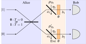
a)

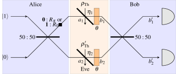
b)

Figure 1: Dual-rail BB84 protocol in the thermal-loss channel. a) and b) show the rectilinear and diagonal polarization bases as the dual-rail equivalent of the BB84 discrete-variable QKD protocol, respectively. Both bases undergo a phase shift $\theta$ with phase noise $\sigma^{2}_{\theta}$. In a), based on which mode (top or bottom) Alice chooses to send a single photon determines the logical bit $\bf{0}$ or $\bf{1}$. In b), based on the phase $0$ or $\pi$ of the rotation $R$ (black square), Alice prepares a logical bit $\bf{0}$ or $\bf{1}$, respectively.

In this section, we present the security models and secret key rate expressions for the DV-QKD and CV-QKD protocols in the thermal-loss channel. We then present the results of the secret key rate of these calculations.

I.1 Thermal-loss in the BB84 (and six-state) dual-rail protocol

We make use of the dual-rail BB84 protocol which is one possible implementation of the original BB84 protocol. In the original BB84 protocol, Alice sends a polarization qubit to Bob with a channel that can support both polarizations. This is equivalent to Alice utilising two quantum channels, each supporting only a single polarization. We present this dual-rail BB84 protocol in Fig. 1 a) and 1 b). In the BB84 protocol, Alice prepares a single qubit in either the rectilinear $Z$-basis $\{\ket{0},\ket{1}\}$ or the diagonal $X$-basis $\{\ket{+},\ket{-}\}$. In the rectilinear basis shown in Fig. 1 a), a logical $\bf{0}$ is prepared by Alice sending a single photon state $\ket{1}$ in the top $a_{1}$ mode and a vacuum state $\ket{0}$ in the bottom $a_{2}$ mode. Similarly, a logical $\bf{1}$ is prepared by sending the vacuum state $\ket{0}$ in the top $a_{1}$ mode and a single-photon state $\ket{1}$ in the bottom $a_{2}$ mode. The qubits pass through a thermal-loss channel represented by a beamsplitter parameter with transmissivity $0\leq\eta_{1,2}\leq 1$ and thermal state $\rho_{\text{Th}}$ with $N_{\text{Th}}$ thermal photons in the auxiliary port.

Bob, after deciding randomly (discussed in detail later) to measure the $Z$-basis, measures each mode output with single-photon detectors, only accepting single-photon events at $b_{1}$ or $b_{2}$ corresponding to logical $\bf{0}$ or $\bf{1}$. Any other detector events are not counted towards the final key. In the diagonal basis (see Fig. 1 b)), Alice interferes with a single-photon with the vacuum using a balanced $50:50$ beamsplitter to generate the superposition state $\ket{+}=\frac{1}{\sqrt{2}}(\ket{1}_{a_{1}}\ket{0}_{a_{2}}+\ket{0}_{a_{1}}\ket{1}_{a_{2}})$ which corresponds to a logical $\bf{1}$ state. A logical $\bf{0}$ corresponds to Alice placing a $\pi$-phase shifter after the beamsplitter and generating the state $\ket{-}=\frac{1}{\sqrt{2}}(\ket{1}_{a_{1}}\ket{0}_{a_{2}}-\ket{0}_{a_{1}}\ket{1}_{a_{2}})$ to send to Bob. Bob, having randomly decided to measure in the $X$-basis by placing a balanced beamsplitter, measures only single-photon events at $b^{\prime}_{1}$ or $b^{\prime}_{2}$ corresponding to logical $\bf{0}$ or $\bf{1}$. We assume the modes pass through the thermal-loss channels with $\eta_{1}=\eta_{2}=\eta$ and thermal noise $N_{\text{Th}}$ and no correlations between the two thermal environments. In the final step of the protocol, Bob sends information to Alice about which basis he used. In this reconciliation phase, Alice discards the data that does not match the basis she used to encode her qubits.

The key rate (per channel use) for the BB84 protocol with perfect reconciliation efficiency in the asymptotic limit is Shor and Preskill (2000); Renner (2008); Murta et al. (2020)

$$K_{\text{BB84}}=\frac{P_{S}}{2}(1-h(Q_{Z})-h(Q_{X})),$$ (1)

where $h(x)=-x\log_{2}{(x)}-(1-x)\log_{2}{(1-x)}$ is the binary entropy function, $P_{S}$ is the success probability of single-photon events, $Q_{Z}$ and $Q_{X}$ are the quantum bit error rates (QBERs) of the measurement bases $Z$ and $X$ respectively. Unlike the usual normalization preserving DV channels, the success probability $P_{S}$ is necessary because the thermal environment adds Gaussian noise, and only single-photon events are counted towards the secret key rate. Here, we assume perfect number-resolving detectors as opposed to click detectors that count all non-vacuum $n>0$ events.

To calculate $Q_{Z}$, we consider the probability of a bit-flip if Alice sends a logical $\bf{0}$ (i.e. $\ket{1}_{a_{1}}\ket{0}_{a_{2}}$) and Bob detects a logical $\bf{1}$ (i.e. simultaneously detects $\ket{0}_{b_{1}}$ and $\ket{1}_{b_{2}}$) with probability given by (see Appendix A for full calculations):

$$\begin{split}P_{Z,\bf{0}\rightarrow\bf{1}}&=P_{Z,\ket{0}_{a_{1}}\rightarrow\ket{1}_{b_{1}}}P_{Z,\ket{1}_{a_{2}}\rightarrow\ket{0}_{b_{2}}}\\ &=\frac{\,N_{\text{Th}}(1+N_{\text{Th}})(1-\eta)^{2}}{\gamma^{4}},\end{split}$$ (2)

where $\gamma=1+N_{\text{Th}}-N_{\text{Th}}\eta$.

Bob only accepts the correct bits and the flipped bits using photon-number resolving detectors. Therefore, we normalize by considering the total probability Bob only detects the logical bits in the $Z$-basis. Since we assume the channels are symmetric, $P_{Z,\bf{1}\rightarrow\bf{0}}=P_{Z,\bf{0}\rightarrow\bf{1}}$, the QBER is

$$Q_{Z}=\frac{P_{Z,\bf{0}\rightarrow\bf{1}}}{P_{Z,\bf{0}\rightarrow\bf{1}}+P_{Z,\bf{0}\rightarrow\bf{0}}}=\frac{P_{Z,\bf{1}\rightarrow\bf{0}}}{P_{Z,\bf{1}\rightarrow\bf{0}}+P_{Z,\bf{1}\rightarrow\bf{1}}},$$ (3)

where $P_{Z,\bf{0}\rightarrow\bf{0}}=P_{Z,\ket{1}_{a_{1}}\rightarrow\ket{1}_{b_{1}}}P_{Z,\ket{0}_{a_{2}}\rightarrow\ket{0}_{b_{2}}}$ and $P_{Z,\bf{1}\rightarrow\bf{1}}=P_{Z,\ket{0}_{a_{1}}\rightarrow\ket{0}_{b_{1}}}P_{Z,\ket{1}_{a_{2}}\rightarrow\ket{1}_{b_{2}}}$ are the probabilities of Bob detecting the same bits that Alice sent after passing through the channel. The probability of an event (or success) is given by:

$$\begin{split}P_{S}&=P_{Z,\bf{0}\rightarrow\bf{1}}+P_{Z,\bf{0}\rightarrow\bf{0}}\\ &=\frac{\eta+2\,N_{\text{Th}}(1+N_{\text{Th}})(1-\eta)^{2}}{\gamma^{4}}.\end{split}$$ (4)

To calculate $Q_{X}$, we consider the bit-flips in the $X$ basis. In this case, the modes $a_{1}$ and $a_{2}$ are entangled because of the balanced beamsplitter (see Fig. 1 b)). Similar to above, we obtain the QBER, for the $X$ bases as

$$Q_{X}=\frac{P_{X,\bf{0}\rightarrow\bf{1}}}{P_{X,\bf{0}\rightarrow\bf{1}}+P_{X,\bf{0}\rightarrow\bf{0}}}.$$ (5)

We find due to symmetry that the probabilities for the diagonal basis are the same as for the rectilinear basis and it follows that $Q_{X}=Q_{Z}$, simplifying the key rate equation. We make use of Eqs. (1), (5), and (4) to calculate the key rate in the asymptotic limit.

Conditioned on the outcome with probability $P_{S}$, it can be shown that the density matrix after the thermal-loss channel is, in fact, a depolarized state (see Appendix B):

$$\begin{split}\tilde{\rho}^{B}:=\frac{\rho^{B}}{P_{S}}&=\frac{\eta}{\eta+2\,N_{\text{Th}}(1+N_{\text{Th}})(1-\eta)^{2}}\rho^{A}\\ &+\frac{N_{\text{Th}}(1+N_{\text{Th}})(1-\eta)^{2}}{\eta+2\,N_{\text{Th}}(1+N_{\text{Th}})(1-\eta)^{2}}\mathbb{I},\end{split}$$ (6)

where $\rho^{A}$ is Alice’s initial density matrix. This represents a depolarizing channel Wilde (2017)

$$\rho\to(1-\lambda)\rho+\frac{\lambda}{2}\mathbb{I}$$ (7)

with depolarizing parameter

$$\lambda=\frac{2\,N_{\text{Th}}(1+N_{\text{Th}})(1-\eta)^{2}}{\eta+2\,N_{\text{Th}}(1+N_{\text{Th}})(1-\eta)^{2}},$$ (8)

which tends to 1 as $\eta\to 0$ or $N_{\text{Th}}\to\infty$, as expected.

A property of the depolarizing channel is that the error rate is the same in all bases:

$$Q_{X,Y,Z}=\frac{\lambda}{2}=\frac{N_{\text{Th}}(1+N_{\text{Th}})(1-\eta)^{2}}{\eta+2N_{\text{Th}}(1+N_{\text{Th}})(1-\eta)^{2}},$$ (9)

which can be seen from Eq. (7). In establishing this equivalence between the thermal-loss and depolarizing channel, we extend our analysis to the six-state protocol which makes use of an additional basis $Y$ with QBER $Q_{Y}$. The key rate for the 6S protocol is given by Murta et al. (2020):

$$K_{\text{6S}}=\frac{P_{S}}{2}(1-H(\Lambda_{00})-H(\Lambda_{01})-H(\Lambda_{10})-H(\Lambda_{11})),$$ (10)

where $H(x)=-x\log_{2}{x}$, and

$$\begin{split}\Lambda_{00}&=1-\frac{Q_{X}+Q_{Y}+Q_{Z}}{2},\\ \Lambda_{01}&=\frac{Q_{X}+Q_{Y}-Q_{Z}}{2},\\ \Lambda_{10}&=\frac{-Q_{X}+Q_{Y}+Q_{Z}}{2},\\ \Lambda_{11}&=\frac{Q_{X}-Q_{Y}+Q_{Z}}{2},\end{split}$$ (11)

where the factor of $1/2$ is to normalize the key-rate to per channel use. In the thermal-loss channel, the QBER $Q_{X}=Q_{Y}=Q_{Z}$ is symmetric. However, as we will see when phase noise is introduced, the QBER of the three bases can be asymmetric.

Lower bounds of BB84 and 6S protocols in the thermal-loss channel

Introducing random bit flips at Alice before the error processing increases the performance of BB84 in a noisy channel and sets a tighter lower bound on the key rate Renner et al. (2005). In this extension of the BB84 protocol which we denote as NBB84, the key rate equation depends on Alice’s added bit-flip probability $q$ (or trusted bit-flips). Following Ref. Renner et al. (2005), we make use of the QBER for the thermal-loss channel in Eq. (54) and maximize the key rate with respect to $q$. We note that the six-state protocol (with and without trusted bit-flips) can tolerate higher QBER than the BB84 protocol Renner et al. (2005). Similarly, the lower bound on the secret key rate of the 6S protocol is likewise calculated by introducing bit-flips at Alice which increases the QBER tolerance of the channel Renner et al. (2005).

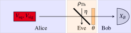
a)

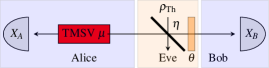
b)

Figure 2: Squeezed-state protocol with homodyne detection in the thermal-loss channel. The phase shifter $\theta$ represents the phase noise $\sigma_{\theta}^{2}$. Shown in a) is the equivalent prepare and measure squeezed-state protocol and in b) is the entanglement-based version of the squeezed-state protocol.

I.2 Thermal-loss in the squeezed state protocol

In the squeezed-state protocol in a prepare-and-measure (PM) scheme presented in Fig. 2 a), Alice introduces a modulation signal in either the $X=\hat{a}+\hat{a}^{\dagger}$ or $P=-i(\hat{a}-\hat{a}^{\dagger})$ quadrature (randomly chosen) a squeezed state with $V_{\text{sq}}$ with Gaussian distribution centered at $0$ with variance $V_{\text{sig}}$. In the equivalent entanglement-based (EB) scheme presented in Fig. 2 b), Alice performs a homodyne measurement on one mode of a shared two-mode squeezed vacuum state (TMSV) where the other mode passes through the channel $\mathcal{E}$, and Bob performs a homodyne measurement Sańchez (2007). The parameter transformation between the PM and EB schemes is:

$$\begin{split}V_{\text{sq}}&=1/\mu,\\ V_{\text{sig}}&=\frac{\mu^{2}-1}{\mu},\end{split}$$ (12)

where $\mu$ is the quadrature variance of $X$ and $P$ of the TMSV source in EB scheme. The following key rate calculations are in the EB scheme. In the asymptotic regime of infinite keys, Eve’s most powerful attack is a collective attack. Security proofs in this regime for this protocol are based on reduction of coherent attacks to collective attacks for infinite dimensions and on the optimality of Gaussian attacks Wolf et al. (2006); García-Patrón and Cerf (2006); Navascués et al. (2006). The secret key rate against collective attacks in the asymptotic regime with reverse reconciliation is given by Laudenbach et al. (2018)

$$K_{\text{RR}}=\beta I_{\text{AB}}-\chi_{\text{EB}},$$ (13)

where $\beta$ is the reconciliation efficiency, $I_{\text{AB}}$ is the mutual information between Alice and Bob, and $\chi_{\text{EB}}$ is the Holevo information between Bob and Eve. In a Gaussian thermal-loss channel, the quadrature covariance matrix between Alice and Bob is Sańchez (2007):

$$\begin{split}&\gamma_{\rm AB}=\begin{pmatrix}a\mathbb{I}&c\sigma_{z}\\ c\sigma_{z}&b\mathbb{I}\end{pmatrix}=\begin{pmatrix}\gamma_{\text{A}}&\sigma_{\text{AB}}\\ \sigma_{\text{AB}}&\gamma_{\text{B}}\end{pmatrix}=\\ &\begin{pmatrix}(V_{\text{A}}+1)\mathbb{I}&\sqrt{\eta(V_{\text{A}}^{2}+2V_{\text{A}})}\sigma_{z}\\ \sqrt{\eta(V_{\text{A}}^{2}+2V_{\text{A}})}\sigma_{z}&V_{B}\mathbb{I}\end{pmatrix},\end{split}$$ (14)

where $V_{\text{A}}=\mu-1$ and $V_{B}=\eta(V_{\text{A}}+1)+(1-\eta)(2N_{\text{Th}}+1)$ are the TMSV variances measured by Alice and Bob (respectively), $\mathbb{I}=\text{diag}(1,1)$ is the unity matrix and $\sigma_{z}\leavevmode\nobreak\ =\leavevmode\nobreak\ \text{diag}(1,-1)$ is the Pauli-Z matrix. We choose homodyne detection (also known as “switching") at Bob, in which Bob switches between $X$ or $P$ quadrature measurements.

In the squeezed state protocol with homodyne detection, the mutual information is given by:

$$I_{\text{AB}}^{\text{hom}}=\frac{1}{2}\log_{2}{\Big{(}\frac{V_{\text{B}}}{V_{\text{B|A}}}\Big{)}},$$ (15)

where $V_{\text{B|A}}=b-\frac{c^{2}}{a}$. The Holevo information between Bob and Eve for the collective attack is given by

$$\chi_{\text{EB}}=S(\text{E})-S(\text{E|B}),$$ (16)

where $S(\text{E})$ is Eve’s information and $S(\text{E|B})$ is Eve’s information conditioned on Bob’s measurement. In Eve’s collective attack, Eve holds a purification of the state between Alice and Bob with entropy given by

$$S(\text{E})=S(\text{AB})=G[(\lambda_{1}-1)/2]+G[(\lambda_{2}-1)/2],$$ (17)

where $G(x)=(x+1)\log_{2}{(x+1)}-x\log_{2}{x}$ and $\lambda_{1,2}$ are the symplectic eigenvalues of the covariance matrix $\gamma_{\text{AB}}$ given by $\lambda_{1,2}^{2}=\frac{1}{2}[\Delta\pm\sqrt{\Delta^{2}-4\mathcal{D}^{2}}]$, where $\Delta=\text{Det}(\gamma_{\text{A}})+\text{Det}(\gamma_{\text{B}})+2\text{Det}(\sigma_{\text{AB}})$, and $\mathcal{D}=\text{Det}(\gamma_{\text{AB}})$. The conditional covariance matrix of Alice’s mode after the homodyne detection by Bob is

$$\Gamma_{\text{A}|b}=\begin{pmatrix}\mu-\frac{\eta(\mu^{2}-1)}{\eta\mu+(1-\eta)(2N_{\text{Th}}+1)}&0\\ 0&\mu\end{pmatrix}.$$ (18)

Therefore, Eve’s entropy conditioned on Bob’s measurement $S(\text{E|B})=S(\text{A}|b)$ is given by $G[(\lambda_{3}-1)/2]$ where $\lambda_{3}$ is the symplectic eigenvalue of $\Gamma_{A|b}$.

Introducing trusted noise before Bob’s homodyne measurement can help extend a high-noise thermal-loss channel. In this extension of the squeezed-state protocol which we denote NSqz-Hom, trusted Gaussian noise $\xi_{\text{B}}$ is added before post-processing on Bob’s homodyne measurement data Sańchez (2007). The effect is that Eve’s information decreases more than the mutual information between Alice and Bob (see Appendix C for calculations), thus increasing the secret key rate of the protocol. Similarly, heterodyne detection at Bob has the same effect of introducing additional noise, thereby extending secure communication distance in a thermal-loss channel García-Patrón and Cerf (2009).

II Phase noise in QKD

We consider a standard model of bosonic phase noise, known also as dephasing, phase-diffusion, or phase-damping; for an excellent review, see Lami and Wilde (2022). This channel represented by $\theta$ on the right of Fig. 1 applies rotation by a random angle $\theta$ to the bosonic state according to a classical distribution $f(\theta)$, giving the transformation

$$\rho\longmapsto\int_{-\pi}^{\pi}d\theta f(\theta)e^{i\hat{a}^{{\dagger}}\hat{a}\theta}\rho e^{-i\hat{a}^{{\dagger}}\hat{a}\theta}.$$ (19)

Since $\hat{a}^{{\dagger}}\hat{a}$ is the number operator, a given rotation $\theta$ applies a phase $e^{in\theta}$ to each Fock state $\ket{n}$, equivalently described by the transformation

$$\hat{a}^{{\dagger}}\longmapsto e^{i\theta}\hat{a}^{{\dagger}}.$$ (20)

The canonical phase distribution is the wrapped normal distribution, which models the random diffusion of an angle and accurately represents the physical process of phase diffusion Lami and Wilde (2022). Birefringence may produce this behaviour in polarisation-based implementations of the six-state and BB84 protocols or in time-bin implementations, phase drift in between the interferometers at either end Lamoureux et al. (2005).

The phase shift $\theta$ (assumed here to have mean zero) is normally distributed over the whole real line:

$$\tilde{f}_{WN}(\theta)=\frac{1}{\tilde{\sigma}\sqrt{2\pi}}e^{-\theta^{2}/2\tilde{\sigma}^{2}}:\qquad\theta\in\mathbb{R},$$

which we can ‘wrap’ into a single $2\pi$ interval by summing the contributions from equivalent angles:

$$f_{WN}(\theta)=\frac{1}{\tilde{\sigma}\sqrt{2\pi}}\sum_{k=-\infty}^{\infty}e^{-(\theta+2\pi k)^{2}/2\tilde{\sigma}^{2}}:\theta\in[-\pi,\pi].$$

The variance $\tilde{\sigma}^{2}$ of $\theta$ over the whole real line is in general not its variance when wrapped; however, the two distributions approach each other in the limit of small variance.

The corresponding qubit transformation of the phase noise ignoring the thermal-loss ($\eta=1$) is $\rho_{jk}\mapsto e^{i\theta_{j}}e^{-i\theta_{k}}\rho_{jk}$, which may be expressed as $\rho\rightarrow\hat{U}_{\bm{\theta}}\rho\hat{U}_{\bm{\theta}}^{{\dagger}}$ where $\hat{U}_{\bm{\theta}}=\operatorname{diag}(e^{i\theta_{i}},e^{i\theta_{j}})$. If $\bm{\theta}$ is drawn from a distribution $f(\bm{\theta})$, the qubit channel becomes

$$\rho\to\langle\hat{U}_{\bm{\theta}}\rho\hat{U}_{\bm{\theta}}^{{\dagger}}\rangle=\int_{\bm{\theta}}f(\bm{\theta})\hat{U}_{\bm{\theta}}\rho\hat{U}_{\bm{\theta}}^{{\dagger}}\;d\bm{\theta}$$

where $\langle\cdot\rangle$ denotes expected value. If $\{\theta_{j}\}$ are independent, the corresponding transformation of off-diagonal terms ($i\neq j$) is

$$\rho_{jk}\longmapsto\langle e^{i\theta_{j}}e^{-i\theta_{k}}\rangle\rho_{jk}=\langle e^{i\theta_{j}}\rangle\langle e^{-i\theta_{k}}\rangle\rho_{jk}=r_{j}r_{k}^{*}\rho_{jk}$$

where $r_{j}:=\langle e^{i\theta_{j}}\rangle$ is the so-called ‘circular mean’ of $\theta_{j}$, given for the wrapped normal distribution:

$$r_{j}=e^{-\tilde{\sigma}^{2}/2}.$$ (21)

Diagonal entries remain unchanged:

$$\rho_{jj}\longmapsto\langle e^{i\theta_{j}}e^{-i\theta_{j}}\rangle\rho_{jj}=\rho_{jj}.$$

If $\{\theta_{j}\}$ are identically distributed then all have the same (real) circular mean $r$ and we obtain a (generalised) dephasing channel Wilde (2017)

$$\rho\longmapsto\rho_{\text{dephased}}=\begin{bmatrix}\rho_{00}&r^{2}\rho_{01}\\ r^{2}\rho_{10}&\rho_{11}\end{bmatrix}$$ (22)

which always sends single-photon inputs to single-photon outputs, unlike the thermal-loss channel. By leaving diagonal entries unchanged, Eq. (22) introduces no error in the Z basis. Common DV-QKD protocols such as the (generalised) BB84 and six-state protocols make use of additional bases ($X$ and $Y$) which are unbiased with respect to the Z basis.

The extension to the combined thermal-loss phase-noise rail presented in Fig. 1 can be obtained by composing the separate depolarization and dephasing channels described in Eqs. (7) and (22), giving

$$\rho\longrightarrow(1-\lambda)\begin{bmatrix}\rho_{00}&r^{2}\rho_{01}&\\ r^{2}\rho_{10}&\rho_{11}\end{bmatrix}+\frac{\lambda}{2}\mathbb{I}.$$

The corresponding error rates are thus $(1-\lambda)\rho_{\mathrm{dephased}}+\frac{\lambda}{2}\mathbb{I}$, i.e.

$$Q_{Z} =\left(\frac{\lambda}{2}\right),$$ (23)

$$Q_{X,Y} =\left(\frac{1}{2}\right)\left[(1-\lambda)(1-r^{2})+\lambda\right],$$

with $r^{2}$ and $\lambda$ given by Eqs. (21) and (8) respectively. The probability of success $P_{S}$ remains the same as for the thermal-loss channel in Eq. (4), as the subsequent dephasing does not affect which states are discarded. The key rate for the BB84 and 6S protocols are straightforward to calculate from these QBERs and using Eqs. (1) and (10), respectively.

For CV-QKD, we make use of the phase noise model shown in Ref. Qi et al. (2015); Marie and Alléaume (2017); Laudenbach et al. (2018); Tang et al. (2020). Residual phase noise manifests as an added excess noise that Bob measures given by:

$$\epsilon_{\theta}=2V_{A}(1-e^{-V_{\theta}/2}),$$ (24)

where $V_{\theta}$ is the phase noise between the local oscillator and signal. Since the squeezed-state protocol is modulated with equal probability in the $X$ or $P$ quadratures, the excess noise due to phase noise is symmetric Sańchez (2007). In Appendix D, we show that the phase noise associated with the squeezing angle of $\phi$ and the phase noise associated with the coherent state phase of $\theta$ can be incorporated into the same phase noise parameter. Application of the rotation operators on squeezed coherent states leads to the same excess noise in Eq. (24). Finally, we assume that the Gaussian phase noise in CV-QKD $V_{\theta}$ is equal to the wrapped normal distribution variance $\sigma^{2}_{\theta}$ in DV-QKD. We note that in the regime where $\sigma^{2}_{\theta}$ is large, the phase diffusion channel becomes non-Gaussian Lami and Wilde (2022). Since we are considering the squeezed-state protocol with coherent detection, we make use of Eq. (16) to calculate a lower bound on the key rate. It is left for future work to determine optimal protocols in the phase diffusion channel.

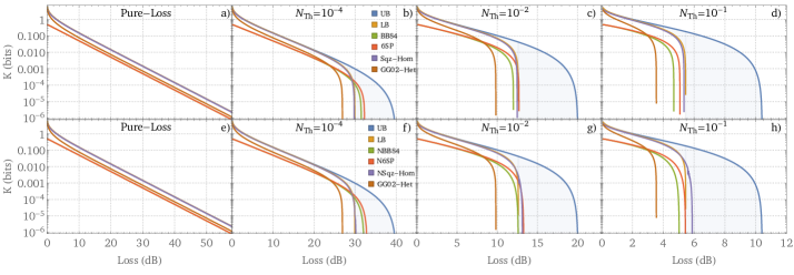
Figure 3: Secret key rate per polarization channel in a thermal-loss channel for increasing noise $N_{\text{Th}}$. Figures a)-d) and e)-h) show the QKD versions of the protocols without and with trusted noise, respectively. For comparison, we also include the GG02 in all figures. For the pure-loss channel, the Sqz-Hom and NSqz-Hom essentially overlap with the PLOB bound for the chosen squeezing of $15\leavevmode\nobreak\ \text{dB}$. Next in b) and f) with some noise in the thermal-loss channel means that the BB84, NBB84, 6S and N6S protocols outperform the CV-QKD protocols. As shown in c), d), g) and h) as more thermal noise is present, the Sqz-Hom and NSqz-Hom outperform BB84, NBB84, 6S, and N6S. In particular, Sqz-Hom saturates the lower bound (LB). Lastly, NSqz-Hom is by far the best protocol in a high noise regime as shown in h) but far from the upper bound (UB).

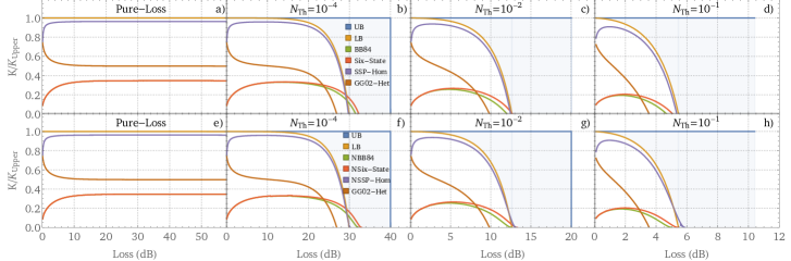
Figure 4: Same as Fig. 3 but to benchmark the performance of the different protocols, we normalise the key rates by the upper bound $K_{\text{Upper}}$.

III Comparison of QKD protocols

III.1 Without phase noise $\sigma_{\theta}^{2}=0$

In CV-QKD, information is encoded in the $X$ and/or $P$ quadratures in one polarization with access to an infinite Hilbert space. Conversely, in DV-QKD, information is encoded in one or more polarization basis in a $2$-dimensional Hilbert space. To make a fair comparison, we assume that Alice uses one polarization basis asymptotically close to $100\%$ of the time (the "computational" basis). The other basis is only measured to characterize channel parameters and the QBER. We make a similar assumption for the squeezed state protocols in the sense that Bob rarely switches the quadrature he measures to characterize the anti-squeezing and determine whether Eve tampered with the shared EPR state, thus removing the usual sifting factor of $1/2$ that comes with switching.

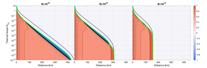
Figure 5: Comparison of $\tilde{K}^{\text{CV:DV}}$ for protocols for a set of thermal-loss channel parameters. Blue regions indicate where the 6S protocol has a higher key rate than Sqz-Hom and conversely, red regions are where the Sqz-Hom has higher key rates than the 6S protocol. Given a minimum key rate requirement, we compare the protocols which operate the best for single-channel use QKD. The 6S protocol covers a small region of intermediate noise and loss as seen in the first two subfigures. The green line indicates where the QKD protocols can operate up to the minimum key rate. The rest of the parameter space is covered by the squeezed state protocol. For high key rates in the rightmost subfigure, the 6S protocol always performs worse than Sqz-Hom. The purple line is the upper bound (UB) of the key capacity in the thermal-loss channel. The red region in the middle and right subfigures are regions where only the Sqz-Hom can achieve the minimum key rate.

We also make the following ideal assumptions about the CV-QKD and DV-QKD protocols in the thermal-loss channel: (i) single-photon and laser sources are perfect (ii) detectors that are used are ideal with detector efficiencies $\eta_{\text{d}}=1$ and detector noise $\xi_{\text{det}}=0$ (except for intentionally adding trusted noise in the “fighting noise with noise" protocol) (iii) all channel parameters have been estimated with no statistical error (iv) all channel noise is attributed to Eve (v) reverse reconciliation efficiency is perfect with $\beta=1$ and error correction efficiency is perfect for both CV-QKD and DV-QKD (vi) all security analysis is in the asymptotic limit. Our simplified analysis here is valid in the ideal situation where squeezed and coherent states are only affected by loss, thermal noise and (in the next section) phase noise.

Pirandola et. al determined lower bounds (LB) and upper bounds (UB) on the secret key capacity $C(\eta,N_{\text{Th}})$ of the thermal loss channel where $N_{\text{Th}}$ is the thermal noise and $\eta$ is the transmissivity of the thermal-loss channel Pirandola et al. (2017, 2009). The lower bound is given by the reverse coherent information of the thermal-loss channel and the upper bound by the Gaussian relative entropy of entanglement (of the Choi state in the thermal-loss channel):

$$\begin{split}&C(\eta,N_{\text{Th}})\geq-\log_{2}{[1-\eta]}-G(N_{\text{Th}})=K_{\text{Lower}},\\ &C(\eta,N_{\text{Th}})\leq-\log_{2}{[(1-\eta)\eta^{N_{\text{Th}}}]}-G(N_{\text{Th}})\\ &\qquad\qquad\qquad\qquad\qquad\qquad\qquad\qquad=K_{\text{Upper}},\end{split}$$ (25)

given for non-entanglement breaking channels $N_{\text{Th}}<\eta/(1-\eta)$ and where $G(x)=(x+1)\log_{2}{(x+1)}-x\log_{2}{x}$.

We present our results in Fig. 3 a)-d) for the secret key rate per polarization channel based on calculations of the BB84 protocol, the 6S protocol, the GG02 protocol (see Appendix E calculations), and the squeezed state with homodyne (Sqz-Hom) protocols in the thermal-loss channel for various thermal noise parameters. We note that since we make use of the dual-rail BB84 protocol which is one possible implementation of the BB84 protocol, the key rate equation for the DV-QKD protocols has been divided by $2$ into units of symbols per polarization channel. For the Sqz-Hom protocol, we choose a practically achievable squeezing $V_{\text{sq}}$ of $15$ dB Vahlbruch et al. (2016). We note that adding more squeezing only adds a very small improvement to the key rates (see Appendix F for more details). In the limit of infinite squeezing, the secret key rate of the Sqz-Hom would approach the lower bound (LB) of the secret key capacity in the thermal-loss channel as shown most clearly in Fig. 3 b) and in a pure-loss channel as shown in Fig. 3 a). The BB84 and 6S protocols surpass the lower bound in an intermediate thermal-noise regime as shown in Fig. 3 b). In Fig. 3 e)-h), we present the “fighting noise with noise" versions of the protocols. For the squeezed state protocol with homodyne detection (NSqz-Hom) with $15$ dB squeezing we optimized with respect to the trusted noise $\xi_{B}$. As shown in Fig. 3 g) and h) surpasses the LB for high thermal noise. In addition, the secret key rate of the “fighting noise with noise" versions of the DV-QKD protocols, the NBB84 and N6S protocols are optimized with respect to the added bit-flips by Alice $q$ and a slight advantage is obtained as shown in Fig. 3 c). In Fig. 4, to benchmark the performance of the different protocols, we normalized the key rate to the upper bound of the secret key capacity.

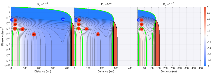
(a) Contour plot of $\tilde{N}_{\text{Th}}^{\text{CV:DV}}$ as a function of the phase noise and distance (or loss) for the Sqz-Hom and 6S protocol. The green line indicates the point at which both protocols tolerate the same amount of thermal noise. In the white regions to the right-hand side, neither one of the protocols tolerate any thermal noise. In the red region, only the Sqz-Hom protocol tolerates thermal noise. We also show current state-of-the-art CV-QKD (red asterisks) and DV-QKD (blue circles) protocols.

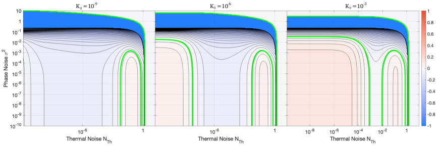
(b) Contour plot of $\tilde{L}^{\text{CV:DV}}$ or $\tilde{D}^{\text{CV:DV}}$ as a function of the phase noise and thermal noise for the Sqz-Hom and 6S protocol. The green line indicates the point at which both protocols tolerate the same amount of loss. In the white regions to the right-hand side, neither one of the protocols tolerate any loss.

Figure 6:

We compare the protocols by plotting the parameter:

$$\tilde{K}^{\text{CV:DV}}=\frac{K_{\text{Sqz-Hom}}-K_{\text{6S}}}{\text{Max}[K_{\text{Sqz-Hom}},K_{\text{6S}}]},$$ (26)

for channel parameters of standard optical fibre of loss $0.2\leavevmode\nobreak\ \text{dB/km}$ with distance $D=10^{-\frac{\eta}{50}}\leavevmode\nobreak\ \text{ km}$ and $N_{\text{Th}}$ in Fig. 5. The key rate $(K_{\text{Sqz-Hom}},K_{\text{6S}})>K_{0}$ where $K_{0}$ is the minimum required key rate. When the squeezed-state protocol is significantly higher in key rates $\tilde{K}=1$, and conversely, when the 6S protocol is best, $\tilde{K}=-1$.

In Fig. 5, from left to right, the protocols are operated at increasingly higher key rates. Given a minimum key rate requirement, we compare the protocols which operate the best in bits per channel use. The main observation here is that the channel parameter space where the 6S protocol dominates shrinks for increasingly higher key rates and CV-QKD is at an advantage. It can also be seen that for higher minimum key-rate requirements, only the Sqz-Hom protocol can operate (see red regions in the middle and right subfigures). However, the 6S protocol can be operated in an intermediate-noise regime at low-key rates where CV-QKD cannot (left and centre subfigure).

Our results indicate that common QKD protocols are far from the upper bound secret key capacity in a thermal-loss channel. We also find that the NSqz-Hom protocol has the best excess noise tolerance in very noisy channels in agreement with Ref. Pirandola et al. (2018) but we find that the BB84 and 6S protocols perform better in an intermediate noise regime.

III.2 With phase noise $\sigma^{2}_{\theta}>0$

In the following section, we quantify the performance of the 6S and Sqz-Hom (with optimized modulation variance $V_{A}$) protocols in the combined thermal-loss and phase noise channel. First, consider the maximum tolerable thermal noise given by:

$$\begin{split}&N_{\text{Th}}^{\text{(Max)}}\\ &=\text{arg}N_{\text{Th}}\begin{cases}&0,\qquad\text{if }K(0,\sigma_{\theta}^{2},D)<K_{0}.\\ &K(N_{\text{Th}},\sigma_{\theta}^{2},D)=K_{0},\text{ otherwise. }\end{cases}\end{split}$$ (27)

In other words, the maximum tolerable noise if the key rate is less than $K_{0}$ at $N_{\text{Th}}=0$ is $0$. Otherwise, the maximum tolerable noise is $N_{\text{Th}}$ when the key rate falls to $K_{0}$.

In Fig. 6 a), we plot the following quantity:

$$\begin{split}&\tilde{N}_{\text{Th}}^{\text{CV:DV}}(\sigma_{\theta}^{2},D)\\ &=\frac{N_{\text{Th,Sqz-Hom}}^{\text{(Max)}}-N_{\text{Th,6S}}^{\text{(Max)}}}{\text{Max}[N_{\text{Th,Sqz-Hom}}^{\text{(Max)}},N_{\text{Th,6S}}^{\text{(Max)}}]},\end{split}$$ (28)

which is the difference between the maximum tolerable thermal noise of the Sqz-Hom and the 6S protocols for a given phase noise $\sigma_{\theta}^{2}$ and distance $D$ to achieve a key rate $K_{0}$. Highlighted in the figure is the green contour where both protocols tolerate the same amount of thermal noise, i.e. $\tilde{N}^{\text{CV:DV}}_{\text{Th}}=0$. For low key rates, it can be seen that the squeezed-state protocol tolerates more thermal noise than the 6S protocol in short channels and when $\sigma_{\theta}^{2}<10^{-3}$. The Sqz-Hom protocol also tolerates more thermal noise than the 6S protocol at longer distances. In this red region, the 6S protocol tolerates zero thermal noise, whereas the Sqz-Hom protocol tolerates some thermal noise. For higher key-rate requirements, although the region of noise tolerance shrinks for both protocols, the Sqz-Hom tolerates proportionally more thermal noise across the phase noise versus distance parameter space.

Next, we consider the maximum distance or maximum tolerable loss given by:

$$\begin{split}&D^{\text{(Max)}}\\ &=\text{arg}D\begin{cases}&0,\qquad\text{if }K(N_{\text{Th}},\sigma_{\theta}^{2},0)<K_{0}.\\ &K(N_{\text{Th}},\sigma_{\theta}^{2},D)=K_{0},\text{ otherwise. }\end{cases}\end{split}$$ (29)

In other words, the maximum distance if the key rate is less than $K_{0}$ at $D=0$ is $0$. Otherwise, the maximum distance is $D$ when the key rate falls to $K_{0}$. In Fig. 6 b), we plot the following quantity:

$$\begin{split}&\tilde{L}^{\text{CV:DV}}(\sigma_{\theta}^{2},N_{\text{Th}})=\tilde{D}^{\text{CV:DV}}(\sigma_{\theta}^{2},N_{\text{Th}})\\ &=\frac{D_{\text{Sqz-Hom}}^{\text{(Max)}}-D_{\text{6S}}^{\text{(Max)}}}{\text{Max}[D_{\text{Sqz-Hom}}^{\text{(Max)}},D_{\text{6S}}^{\text{(Max)}}]},\end{split}$$ (30)

which is the difference between the maximum distance of the Sqz-Hom and the 6S protocols for a given phase noise $\sigma_{\theta}^{2}$ and thermal noise $N_{\text{Th}}$ to achieve a key rate $K_{0}$. The Sqz-Hom protocol can tolerate more loss than the 6S protocol at thermal noise between $10^{-2}$ and $0.9$, and phase noise $\sigma_{\theta}^{2}<10^{-3}$. As found in Lasota et al. (2017), at a small region of high thermal noise, the 6S protocol tolerates more loss than the Sqz-Hom protocol. At higher key-rate requirements, the Sqz-Hom protocol can tolerate more loss compared to the 6S protocol. In fact, it can tolerate as much as $\sigma_{\theta}^{2}=0.05$ for a $K>10^{-3}$ key-rate requirement and $N_{\text{Th}}<10^{-3}$ to perform at a longer distance than the 6S protocol.

From these results, we can conclude that for low key-rate requirements, the 6S protocol clearly dominates a larger region of parameters. However, for high key-rate requirements, the Sqz-Hom protocol dominates most of the parameter space for phase noise less than a phase noise of $\sigma^{2}_{\theta}<10^{-3}$.

CV-QKD
Reference	$\sigma_{\theta}^{2}$
B. Qi et al. Qi et al. (2015)	$4\times 10^{-2}$
T. Wang et al. Wang et al. (2018)	$1.2\times 10^{-3}$
H. Wang et al. Wang et al. (2020)	$\leq 7.0\times 10^{-3}$
H.-M. Chin et al. Chin et al. (2021) & A. A. Hajomer et al. Hajomer et al. (2022)	$\text{ }\leq 1.0\times 10^{-3}$
Y. Zhang et al. Zhang et al. (2020)	$7.4\times 10^{-5}$
DV-QKD
Reference	$\sigma_{\theta}^{2}$
A. Boaron et al. Boaron et al. (2018)	$7.2\times 10^{-2}$
W. Li et al. Li et al. (2023)	$2.2\times 10^{-2}$

Table 1: Residual phase noise of locally generated local oscillator Gaussian modulated CV-QKD schemes in the first table and DV-QKD schemes in the second table. With the exception of Ref. Qi et al. (2015), Wang et al. (2018) & Zhang et al. (2020), the phase noise is upper bounded from the total excess noise.

As a comparison, experimental values for the phase noise in CV-QKD protocols are shown in Table. 1. These are also shown in Fig. 6 a) along with current state-of-the-art DV-QKD protocols Boaron et al. (2018) & Li et al. (2023) (converted to distance in standard fibre). For DV-QKD implementations, we convert the time jitter full width at half maximum $\Delta t_{\text{FWHM}}$) to the phase noise using the following equation:

$$\sigma^{2}_{\theta}=\frac{(2\pi\Delta t_{\text{FWHM}})^{2}}{(2\sqrt{2\ln{2}}\Delta t)^{2}},$$ (31)

where $\Delta t$ is the timing between pulses. This equation converts FWHM to a Gaussian width Caloz et al. (2018) and then to a phase noise (in radians squared). The timing between pulses in both experiments is inversely proportional to the repetition rate $\Delta t=1/f$.

Discussion

We discuss our results with less-than-ideal experimental setups of QKD protocols. In optical fibre, the current distance record for DV-QKD is $421\leavevmode\nobreak\ \text{km}$ in ultralow-loss (ULL) fibre ($0.17\leavevmode\nobreak\ \text{dB/km}$) corresponding to $71.9\leavevmode\nobreak\ \text{dB}$ loss Boaron et al. (2018). A secret key rate of $0.25\leavevmode\nobreak\ \text{bps}$ or equivalently $K=10^{-10}\leavevmode\nobreak\ \text{bits per channel use}$ was obtained using superconducting single-photon detectors at a repetition rate of $2.5\leavevmode\nobreak\ \text{GHz}$. Most recently, a high key rate of $K=4.4\times 10^{-2}$ was demonstrated in $10\leavevmode\nobreak\ \text{km}$ of standard optical fiber for DV-QKD Li et al. (2023). We plot these experimental points normalized to standard optical fiber loss ($0.2\leavevmode\nobreak\ \text{ dB/km}$) in Fig. 6 a). Based on these results, for this similar key-rate requirement $K_{0}=10^{-3}$, CV-QKD would, in theory, be able to achieve the same high key rate and tolerate more noise if the same levels of phase noise are maintained as in Wang et al. (2018) & Wang et al. (2020). Additionally, CV-QKD can extend up to $150\leavevmode\nobreak\ \text{ km}$ as opposed to DV-QKD which cannot tolerate noise beyond $125\leavevmode\nobreak\ \text{ km}$. In the rightmost subfigure in Fig. 6 b), it can be seen that CV-QKD can tolerate more loss than DV-QKD for a large parameter region given a higher key rate requirement.

Nonetheless, in terms of distance, DV-QKD is currently leading the benchmark for QKD with the world record for CV-QKD being more than half the distance in ULL fibre at $202.81\leavevmode\nobreak\ \text{km}$ (or $32.4\leavevmode\nobreak\ \text{dB}$) using the GG02 protocol where a key rate of $K\approx 10^{-6}$ was achieved Zhang et al. (2020). On the other hand, the apparent advantage of CV-QKD is in the efficient encoding of keys per symbol and the faster generation and detection of coherent (or squeezed) states with a much larger block size. Post-processing codes at low signal-to-noise ratio were a bottleneck in CV-QKD until it was recently shown that Raptor-like LPDC codes can maintain a high key extraction rate and high reconciliation efficiency, paving the way for practical and deployable CV-QKD Zhou et al. (2021).

We have also focused mainly on the squeezed-state protocol. Despite renewed interest in the squeezed-state protocol due to its robustness to noise Usenko (2018); Derkach et al. (2020); Hosseinidehaj et al. (2022), the difficulty of modulating and generating stable squeezed coherent states remains. However, entanglement-based versions have been demonstrated Madsen et al. (2012), and sources of highly entangled TMSV states are a promising pathway toward realizing the squeezed-state protocol Wang et al. (2021).

Furthermore, one of the limitations of CV-QKD is currently the maintaining of phase reference using a local oscillator (LO), which needs to be practically solved without compromising unconditional security, in a real-world setting outside of the laboratory Zhang et al. (2020). It can be seen from our results, that although CV-QKD performs well in a high-thermal noise regime, the introduction of phase noise destroys this advantage. For CV-QKD to maintain this advantage, the amount of phase noise must be less than $\sigma^{2}_{\theta}<10^{-3}$. However, we also find that CV-QKD performs best for high minimum key-rate requirements where it can tolerate more thermal noise at longer distances than DV-QKD. The physical reason behind this is that in CV-QKD, more symbols can be sent that will result in a shared key. Conversely, DV-QKD is limited to single photons.

Based on these results, we speculate that the consistent historical performance of DV-QKD protocols is mainly due to robustness to phase noise, which plagues CV-QKD protocols that rely on encoding information in phase as well as amplitude. However, with increasingly more robust carrier phase compensation schemes based on machine learning as in Ref. Chin et al. (2021); Hajomer et al. (2022), phase noise may no longer be a limiting factor in CV-QKD.

We note the limitations of our phase noise model for the squeezed-state protocol. We had assumed that the phase noise is Gaussian, whereas the phase diffusion channel is a non-Gaussian channel Lami and Wilde (2022). It is left for future work to determine the optimal QKD protocol in the phase diffusion channel.

Although current upper bounds on the secret key capacity can serve as a benchmark for QKD protocols, no QKD protocol is currently known to saturate these bounds in the thermal-loss channel. We note that energy-constrained upper bounds in the thermal-loss channel have been recently determined, that would be comparable in energy to common DV-QKD protocols Davis et al. (2018).

IV Conclusion

In this work, we compared DV-QKD and CV-QKD protocols on equal grounds in a thermal-loss channel and we assumed ideal sources and detector performances. We developed analytical formulas for the QBER of the BB84 and six-state protocols in a thermal-loss channel. We introduced the minimum key rate as a metric for QKD performance. We found the squeezed-state protocol dominates most of the channel parameter regimes when there is no phase noise, except for an intermediate-noise regime where the six-state protocol can tolerate more loss and surpasses the lower bound to the secret key capacity. With the addition of phase noise, we find that the overall landscape of the DV-QKD and CV-QKD comparison becomes more complex. Finally, we find DV-QKD is largely unaffected by phase noise, whilst CV-QKD is sensitive but performs better below a threshold phase noise only recently reached in experiments.

Author contributions statement

S. P. K. wrote the paper, and produced the calculations and results, P. G. produced some of the analytical calculations, S. M. A. and P. K. L. conceived the main idea and proofread the manuscript. All authors reviewed the manuscript.

Appendices

A Quantum Bit Error Rate (QBER)

To calculate $Q_{Z}$, we consider the probability of a bit-flip if Alice sends a logical $\bf{0}$ (i.e. $\ket{1}_{a_{1}}\ket{0}_{a_{2}}$) and Bob detects a logical $\bf{1}$ (i.e. simultaneously detects $\ket{0}_{b_{1}}$ and $\ket{1}_{b_{2}}$) given by,

$$\begin{split}&P_{Z,\bf{0}\rightarrow\bf{1}}=P_{Z,\ket{1}_{a_{1}}\rightarrow\ket{0}_{b_{1}}}P_{Z,\ket{0}_{a_{2}}\rightarrow\ket{1}_{b_{2}}}\\ &=\text{Tr}(U_{BS}(\eta)(\ket{1}_{a_{1}}\bra{1}_{a_{1}}\otimes\rho_{\text{Th}})U_{BS}^{\dagger}(\eta)\ket{0}_{b_{1}}\bra{0}_{b_{1}})\\ &\times\text{Tr}(U_{BS}(\eta)(\ket{0}_{a_{2}}\bra{0}_{a_{2}}\otimes\rho_{\text{Th}})U_{BS}^{\dagger}(\eta)\ket{1}_{b_{2}}\bra{1}_{b_{2}}),\end{split}$$ (32)

where $\rho_{\text{Th}}=\sum^{\infty}_{n=0}[{N_{\text{Th}}^{n}}/{(N_{\text{Th}}+1)^{n+1}}]\ket{n}\bra{n}$ is the thermal state with average thermal photon number $N_{\text{Th}}$ and $U_{BS}(\eta)$ is the unitary beamsplitter transformation mixing the thermal environment and the state sent by Alice. If Alice prepares a logical $\bf{1}$ and Bob measures $\bf{0}$, the probability is

$$\begin{split}&P_{Z,\bf{1}\rightarrow\bf{0}}=P_{Z,\ket{0}_{a_{1}}\rightarrow\ket{1}_{b_{1}}}P_{Z,\ket{1}_{a_{2}}\rightarrow\ket{0}_{b_{2}}}\\ &=\text{Tr}(U_{BS}(\eta)(\ket{0}_{a_{1}}\bra{0}_{a_{1}}\otimes\rho_{\text{Th}})U_{BS}^{\dagger}(\eta)\ket{1}_{b_{1}}\bra{1}_{b_{1}})\\ &\times\text{Tr}(U_{BS}(\eta)(\ket{1}_{a_{2}}\bra{1}_{a_{2}}\otimes\rho_{\text{Th}})U_{BS}^{\dagger}(\eta)\ket{0}_{b_{2}}\bra{0}_{b_{2}}),\end{split}$$ (33)

and since we assume the channels are symmetric, $P_{Z,\bf{1}\rightarrow\bf{0}}=P_{Z,\bf{0}\rightarrow\bf{1}}$. The total un-normalized probability of a bit-flip is $2P_{Z,\bf{0}\rightarrow\bf{1}}$.

Bob only accepts the correct bits and the flipped bits. Therefore, we normalize by considering the total probability Bob only detects the logical bits in the $Z$-basis. Hence

$$Q_{Z}=\frac{P_{Z,\bf{0}\rightarrow\bf{1}}}{P_{Z,\bf{0}\rightarrow\bf{1}}+P_{Z,\bf{0}\rightarrow\bf{0}}}=\frac{P_{Z,\bf{1}\rightarrow\bf{0}}}{P_{Z,\bf{1}\rightarrow\bf{0}}+P_{Z,\bf{1}\rightarrow\bf{1}}},$$ (34)

where $P_{Z,\bf{0}\rightarrow\bf{0}}=P_{Z,\ket{1}_{a_{1}}\rightarrow\ket{1}_{b_{1}}}P_{Z,\ket{0}_{a_{2}}\rightarrow\ket{0}_{b_{2}}}$ and $P_{Z,\bf{1}\rightarrow\bf{1}}=P_{Z,\ket{0}_{a_{1}}\rightarrow\ket{0}_{b_{1}}}P_{Z,\ket{1}_{a_{2}}\rightarrow\ket{1}_{b_{2}}}$ are the probabilities of Bob detecting the same bits that Alice sent after passing through the channel. These probabilities are given by

$$\begin{split}&P_{Z,\bf{0}\rightarrow\bf{0}}=P_{Z,\bf{1}\rightarrow\bf{1}}\\ &=\text{Tr}(U_{BS}(\eta)(\ket{1}_{a_{1}}\bra{1}_{a_{1}}\otimes\rho_{\text{Th}})U_{BS}^{\dagger}(\eta)\ket{1}_{b_{1}}\bra{1}_{b_{1}})\\ &\times\text{Tr}(U_{BS}(\eta)(\ket{0}_{a_{2}}\bra{0}_{a_{2}}\otimes\rho_{\text{Th}})U_{BS}^{\dagger}(\eta)\ket{0}_{b_{2}}\bra{0}_{b_{2}}).\end{split}$$ (35)

These probabilities are:

$$P_{Z,\bf{0}\rightarrow\bf{1}} =P_{Z,\bf{1}\rightarrow\bf{0}}=\frac{(1-\eta)^{2}(N_{\text{Th}}+N_{\text{Th}}^{2})}{(1+(1-\eta)N_{\text{Th}})^{4}}$$ (36)

$$P_{Z,\bf{0}\rightarrow\bf{0}} =P_{Z,\bf{1}\rightarrow\bf{1}}=\frac{\eta+(1-\eta)^{2}(N_{\text{Th}}+N_{\text{Th}}^{2})}{(1+(1-\eta)N_{\text{Th}})^{4}}.$$ (37)

To calculate $Q_{X}$, we consider the bit-flips in the $X$ basis. In this case, the modes $a_{1}$ and $a_{2}$ are entangled because of the balanced beamsplitter (see Fig. 1 b)). Therefore, we consider the joint probability given by

$$\begin{split}&P_{X,\bf{0}\rightarrow\bf{1}}\\ &=\text{Tr}[U_{50/50,b_{1}b_{2}}U_{BS,a_{1}}(\eta)U_{BS,a_{2}}(\eta)(\ket{-}_{a_{1},a_{2}}\bra{-}_{a_{1},a_{2}}\otimes\rho_{a_{1},\text{Th}}\otimes\rho_{a_{2},\text{Th}})U_{BS,a_{1}}^{\dagger}(\eta)U_{BS,a_{2}}^{\dagger}(\eta)U_{50/50,b_{1}b_{2}}^{\dagger}M_{\bf{1}}],\\ &P_{X,\bf{1}\rightarrow\bf{0}}\\ &=\text{Tr}[U_{50/50,b_{1}b_{2}}U_{BS,a_{1}}(\eta)U_{BS,a_{2}}(\eta)(\ket{+}_{a_{1},a_{2}}\bra{+}_{a_{1},a_{2}}\otimes\rho_{a_{1},\text{Th}}\otimes\rho_{a_{2},\text{Th}})U_{BS,a_{1}}^{\dagger}(\eta)U_{BS,a_{2}}^{\dagger}(\eta)U_{50/50,b_{1}b_{2}}^{\dagger}M_{\bf{0}}],\end{split}$$ (38)

where $U_{50/50,b_{1}b_{2}}$ is the second balanced beamsplitter unitary, $\ket{-}_{a_{1},a_{2}}\bra{-}_{a_{1},a_{2}}=R_{\pi,a_{1}}\ket{+}_{a_{1},a_{2}}\bra{+}_{a_{1},a_{2}}R^{\dagger}_{\pi,a_{1}}$ is obtained by applying a $\pi$-phase shifter to the state $\ket{+}$, $M_{\bf{1}}=\ket{0}_{b^{\prime}_{1}}\bra{0}_{b^{\prime}_{1}}\otimes\ket{1}_{b^{\prime}_{2}}\bra{1}_{b^{\prime}_{2}}$ is the logical $\bf{1}$ measurement outcome and $M_{\bf{0}}=\ket{1}_{b^{\prime}_{1}}\bra{1}_{b^{\prime}_{1}}\otimes\ket{0}_{b^{\prime}_{2}}\bra{0}_{b^{\prime}_{2}}$. Similar to above, we also renormalize to obtain the QBER,

$$Q_{X}=\frac{P_{X,\bf{0}\rightarrow\bf{1}}}{P_{X,\bf{0}\rightarrow\bf{1}}+P_{X,\bf{0}\rightarrow\bf{0}}}.$$ (39)

We find due to symmetry that the probabilities for the diagonal basis are the same as for the rectilinear basis and it follows that $Q_{X}=Q_{Z}$, simplifying the key rate equation.

B Thermal-loss to depolarized state

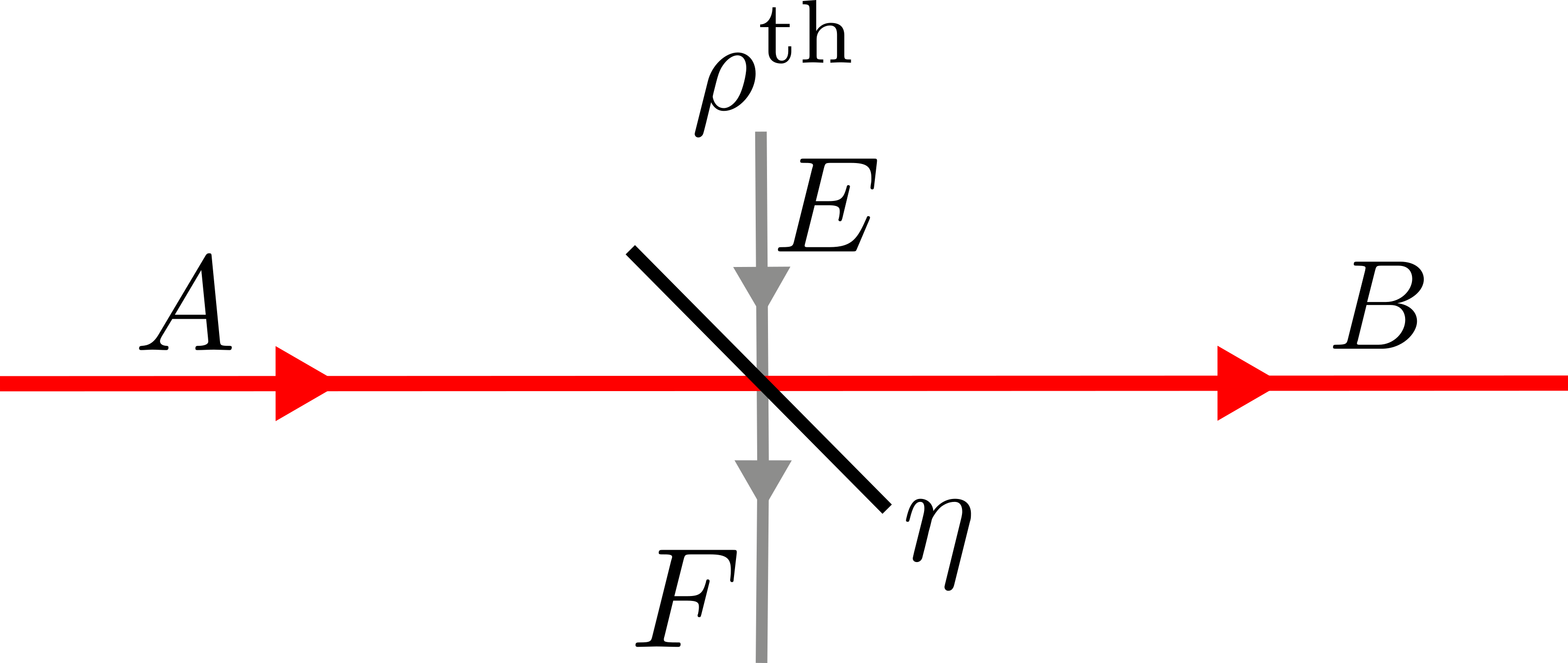
Figure 7: A thermal noise rail with modes labeled for Alice, Bob, and the environment.

Using the model of thermal noise from the previous section we identify Alice’s input mode $A$, Bob’s output mode $B$, and the environmental input and output modes $E$ and $F$ (see Fig. 7), with corresponding creation and annihilation operators (lowercase). A photon-number (Fock) state of a bosonic mode may be expressed as $\ket{n}=\frac{(\hat{a}^{{\dagger}})^{n}}{\sqrt{n!}}\ket{0}$; in this representation, the action of the beamsplitter is given entirely by the transformation

$$\hat{a}\mapsto\sqrt{\eta}\,\hat{b}+\sqrt{1-\eta}\,\hat{f}$$ (40)

$$\hat{e}\mapsto\sqrt{1-\eta}\,\hat{b}-\sqrt{\eta}\,\hat{f}.$$

If the beamsplitter receives no photon from Alice and exactly $n$ photons from the environment, then under action (40) the combined input state $\ket{0,n}_{AE}$ transforms as

$$\ket{0,n}_{AE}=\frac{(\hat{e}^{{\dagger}})^{n}}{\sqrt{n!}}\ket{0,0}_{AE} \longmapsto\frac{(\sqrt{1-\eta}\,\hat{b}^{{\dagger}}-\sqrt{\eta}\,\hat{f}^{{\dagger}})^{n}}{\sqrt{n!}}\ket{0,0}_{BF}$$

$$=\frac{1}{\sqrt{n!}}\left(\sum_{k=0}^{n}\binom{n}{k}(\sqrt{1-\eta}\;\hat{b}^{{\dagger}})^{n-k}(-\sqrt{\eta}\;\hat{f}^{{\dagger}})^{k}\right)\ket{0,0}$$

$$=\frac{1}{\sqrt{n!}}\sum_{k=0}^{n}\frac{n!}{k!(n-k)!}(\sqrt{1-\eta})^{n-k}(-\sqrt{\eta})^{k}\sqrt{(n-k)!}\sqrt{k!}\ket{n-k,k}$$

$$=\sum_{k=0}^{n}\sqrt{\binom{n}{k}}(\sqrt{1-\eta})^{n-k}(-\sqrt{\eta})^{k}\ket{n-k,k}$$

$$:=\ket{\psi_{n}}$$

which is a coherent superposition of Fock states, with $n$ total photons split across rails $B$ and $F$ according to a binomial distribution. If Alice instead sends a single photon we obtain

$$\ket{1,n}_{AE}=\hat{a}^{{\dagger}}\ket{0,n}_{AE} \longmapsto(\sqrt{\eta}\,\hat{b}^{{\dagger}}+\sqrt{1-\eta}\,\hat{f}^{{\dagger}})\ket{\psi_{n}}$$

$$=\sqrt{\eta}\sum_{k=0}^{n}\sqrt{\binom{n}{k}}(-\sqrt{\eta})^{k}(\sqrt{1-\eta})^{n-k}\sqrt{n-k+1}\ket{n-k+1,k}$$

$$\qquad+\sqrt{1-\eta}\sum_{k=0}^{n}\sqrt{\binom{n}{k}}(-\sqrt{\eta})^{k}(\sqrt{1-\eta})^{n-k}\sqrt{k+1}\ket{n-k,k+1}$$

$$:=\ket{\phi_{n}}$$

where the first term corresponds with Alice’s photon reaching Bob, and the second with it escaping to the environment.

It follows that Alice’s input can be considered a $2\times 2$ density matrix $\rho^{A}$ with terms of form $\rho^{A}_{ij}\outerproduct{\mathbf{i}}{\mathbf{j}}$. The collective input $AE$ to the beamsplitter system is therefore

$$\rho^{\mathrm{in}}=\rho^{A}\otimes\rho^{E}=\sum_{i,j,\mathbf{n}}\rho^{A}_{ij}p_{\mathbf{n}}\outerproduct{\mathbf{i},\mathbf{n}}{\mathbf{j},\mathbf{n}}.$$

Since quantum channels are linear, the collective output $BF$ is determined by the action of the channel on each $\outerproduct{\mathbf{i},\mathbf{n}}{\mathbf{j},\mathbf{n}}$ term (despite $\outerproduct{\mathbf{i}}{\mathbf{j}}$ individually representing a nonphysical state whenever $i\neq j$). Since $\ket{\mathbf{i},\mathbf{n}}$ represents an independent input to each beamsplitter, the output is a direct tensor product of the independent single-rail outputs derived above, i.e.

$$\ket{\mathbf{i},\mathbf{n}}_{AE}\longmapsto \ket{\psi_{n_{0}}}_{B_{0}F_{0}}\ket{\psi_{n_{1}}}_{B_{1}F_{1}}\cdots$$

$$\ket{\phi_{n_{0}}}_{B_{0}F_{0}}\cdots\ket{\psi_{n_{1}}}_{B_{n_{1}}F_{n_{1}}}:=\ket{\omega_{\mathbf{i},\mathbf{n}}}_{BF}$$

where only rail $i$ has output $\ket{\phi_{n}}$, the symbol $\omega$ was chosen for no particular reason. The Hermitian conjugate of Eq. (40) transforms the corresponding bra in the same way, giving $\bra{\mathbf{j},\mathbf{n}}\longmapsto\bra{\omega_{\mathbf{j},\mathbf{n}}}$ and hence $\outerproduct{\mathbf{i},\mathbf{n}}{\mathbf{j},\mathbf{n}}\mapsto\outerproduct{\omega_{\mathbf{i},\mathbf{n}}}{\omega_{\mathbf{j},\mathbf{n}}}$. Bob’s final state is

$$\rho^{B}=\Tr_{F}(\rho^{\mathrm{out}})=\Tr_{F}\left(\sum_{i,j,\mathbf{n}}\rho^{A}_{ij}p_{\mathbf{n}}\outerproduct{\omega_{\mathbf{i},\mathbf{n}}}{\omega_{\mathbf{j},\mathbf{n}}}\right)=\sum_{i,j}\rho^{A}_{ij}\sum_{\mathbf{n}}p_{\mathbf{n}}\Tr_{F}\outerproduct{\omega_{\mathbf{i},\mathbf{n}}}{\omega_{\mathbf{j},\mathbf{n}}}$$ (41)

obtained by tracing over the environmental modes in the collective output $\rho^{\mathrm{out}}$.

We assume that Bob may perform a perfect photon-number-resolving (PNR) measurement in any desired basis, and that like Alice he is interested only in single-photon states $\ket{\bm{\beta}}=\sum_{i}\beta_{i}\ket{\mathbf{i}}$ and will discard all others. With perfect measurement, Bob’s outcome probabilities are given by projection:

$$P(\ket{\bm{\beta}})=\expectationvalue{\rho^{B}}{\bm{\beta}}=\Tr(\outerproduct{\bm{\beta}}{\bm{\beta}}\rho^{B})$$ (42)

where only terms of form $\outerproduct{\mathbf{i}}{\mathbf{j}}$ in Bob’s state $\rho^{B}$ contribute to this expression if $\ket{\bm{\beta}}$ is a single-photon state. Like $\rho^{A}$, Bob’s state $\rho^{B}$ may therefore be effectively considered a $2\times 2$ matrix $\rho^{B}_{ij}$, which we now compute. Discarding terms which contain multiple photons in any single one of Bob’s rails leaves

$$\begin{split}\ket{\psi_{n}}&\longrightarrow\ket{\psi_{n}^{\prime}}=(-\sqrt{\eta})^{n-1}\left(-\sqrt{\eta}\ket{0,n}+\sqrt{n(1-\eta)}\ket{1,n-1}\right)\\ \ket{\phi_{n}}&\longrightarrow\ket{\phi_{n}^{\prime}}=(-\sqrt{\eta})^{n-1}\left([n-\eta n-\eta]\ket{1,n}-\sqrt{\eta(1-\eta)(n+1)}\ket{0,n+1}\right).\end{split}$$ (43)

Next, to compute

$$\Tr_{F}\outerproduct{\omega_{\mathbf{i},\mathbf{n}}}{\omega_{\mathbf{j},\mathbf{n}}}=\sum_{\mathbf{n}}\braket{\mathbf{n}}{\omega_{\mathbf{i},\mathbf{n}}}\braket{\omega_{\mathbf{j},\mathbf{n}}}{\mathbf{n}}$$

we need only consider components of $\outerproduct{\omega_{\mathbf{i},\mathbf{n}}}{\omega_{\mathbf{j},\mathbf{n}}}$ with diagonal environmental mode $\outerproduct{\mathbf{n}}{\mathbf{n}}$, as all others vanish. Discarding these nondiagonal terms in each of our single-rail outer products gives

$$\outerproduct{\psi_{n}^{\prime}}{\psi_{n}^{\prime}} \longrightarrow\eta^{n-1}\bigl{(}\eta\outerproduct{0,n}{0,n}+n(1-\eta)\outerproduct{1,n-1}{1,n-1}\bigr{)}$$ (44)

$$\outerproduct{\phi_{n}^{\prime}}{\phi_{n}^{\prime}} \longrightarrow\eta^{n-1}\bigl{(}[n-\eta n-\eta]^{2}\outerproduct{1,n}{1,n}+\eta(1-\eta)(n+1)\outerproduct{0,n+1}{0,n+1}\bigr{)}$$ (45)

$$\outerproduct{\phi_{n}^{\prime}}{\psi_{n}^{\prime}} \longrightarrow-\eta^{n-1}\sqrt{\eta}\,[n-\eta n-\eta]\outerproduct{1,n}{0,n}$$ (46)

$$\outerproduct{\psi_{n}^{\prime}}{\phi_{n}^{\prime}} \longrightarrow-\eta^{n-1}\sqrt{\eta}\,[n-\eta n-\eta]\outerproduct{0,n}{1,n}.$$ (47)

We can decompose $\outerproduct{\omega_{\mathbf{i},\mathbf{n}}}{\omega_{\mathbf{j},\mathbf{n}}}$ in the collective Fock basis as a sum of terms corresponding with each different combination of photon numbers from Eqs. (44) and/or (45). However, we keep only those terms with a photon in exactly one of Bob’s modes; if $i\neq j$, terms (46) and (47) provide these photons (albeit in a different rail on each side of the outer product) and hence all other rails must be empty. After simultaneously tracing out the environment, this gives

$$\Tr_{F}\outerproduct{\omega_{\mathbf{i},\mathbf{n}}}{\omega_{\mathbf{j},\mathbf{n}}}=\frac{1}{\eta}\left(\eta^{n_{i}}[n_{i}-\eta n_{i}-\eta]\right)\left(\eta^{n_{j}}[n_{j}-\eta n_{j}-\eta]\right)\left(\prod_{k\neq i,j}\eta^{n_{k}}\right)\outerproduct{\mathbf{i}}{\mathbf{j}}.$$

If $i=j$, the photon is received either in the original rail $i$ or an erroneous rail $j\neq i$, giving

$$\Tr_{F}\outerproduct{\omega_{\mathbf{i},\mathbf{n}}}{\omega_{\mathbf{i},\mathbf{n}}}=\eta^{n_{i}-1}(n_{i}-\eta n_{i}-\eta)\left(\prod_{k\neq i}\eta^{n_{k}}\right)\outerproduct{\mathbf{i}}{\mathbf{i}}$$

$$+\sum_{j\neq i}(1-\eta)^{2}\,\eta^{n_{i}}(n_{i}+1)\,n_{j}\eta^{n_{j}-1}\left(\prod_{k\neq i,j}\eta^{n_{k}}\right)\outerproduct{\mathbf{j}}{\mathbf{j}}.$$

Returning to Eq. (41), we now sum over all $\mathbf{n}$. This is done analytically, and can also be done with the aid of Mathematica. The resulting action of the channel is defined by

$$\outerproduct{\mathbf{i}}{\mathbf{j}}_{A} \longmapsto\frac{\eta}{\gamma^{4}}\outerproduct{\mathbf{i}}{\mathbf{j}}_{B}:\qquad i\neq j,$$

$$\outerproduct{\mathbf{i}}{\mathbf{i}}_{A} \longmapsto\frac{\eta}{\gamma^{4}}\outerproduct{\mathbf{i}}{\mathbf{i}}+\frac{N_{\text{Th}}(1+N_{\text{Th}})(1-\eta)^{2}}{\gamma^{4}}\mathbb{I}$$

where $\gamma=1+N_{\text{Th}}-N_{\text{Th}}\eta$ and $\mathbb{I}$ is the identity, i.e. $\mathbb{I}/2$ is the maximally-mixed state. Noting that $\Tr\rho^{A}=\sum_{i}\rho^{A}_{ii}=1$, we can thus express this as the qubit transformation $\rho^{A}\to\rho^{B}$ (see Eq. (41)):

$$\rho^{A} \longmapsto\frac{\eta}{\gamma^{2}}\rho^{A}+\frac{N_{\text{Th}}(1+N_{\text{Th}})(1-\eta)^{2}}{\gamma^{2}}\left(\sum_{i}\rho^{A}_{ii}\right)\mathbb{I}$$ (48)

$$=\frac{\eta}{\gamma^{4}}\rho^{A}+\frac{N_{\text{Th}}(1+N_{\text{Th}})(1-\eta)^{2}}{\gamma^{4}}\mathbb{I}.$$ (49)

The trace of this un-normalised output now represents the probability $P_{s}$ of successfully receiving a valid qubit:

$$P_{S}=\Tr\rho^{B}=\frac{\eta+2\,N_{\text{Th}}(1+N_{\text{Th}})(1-\eta)^{2}}{\gamma^{4}}.$$ (50)

Conditional on success, we obtain the normalised state

$$\begin{split}\tilde{\rho}^{B}:=\frac{\rho^{B}}{P_{S}}&=\frac{\eta}{\eta+2\,N_{\text{Th}}(1+N_{\text{Th}})(1-\eta)^{2}}\rho^{A}\\ &+\frac{N_{\text{Th}}(1+N_{\text{Th}})(1-\eta)^{2}}{\eta+2\,N_{\text{Th}}(1+N_{\text{Th}})(1-\eta)^{2}}\mathbb{I}.\end{split}$$ (51)

This represents a depolarizing channel Wilde (2017)

$$\rho\to(1-\lambda)\rho+\frac{\lambda}{2}\mathbb{I}$$ (52)

with depolarizing parameter

$$\lambda=\frac{2\,N_{\text{Th}}(1+N_{\text{Th}})(1-\eta)^{2}}{\eta+2\,N_{\text{Th}}(1+N_{\text{Th}})(1-\eta)^{2}},$$ (53)

which tends to 1 as $\eta\to 0$ or $N_{\text{Th}}\to\infty$, as expected.

A property of the depolarizing channel is that the error rate is the same in all bases:

$$Q=\frac{\lambda}{2}=\frac{N_{\text{Th}}(1+N_{\text{Th}})(1-\eta)^{2}}{\eta+2N_{\text{Th}}(1+N_{\text{Th}})(1-\eta)^{2}},$$ (54)

which can be seen from Eq. (52). In this article, we only focus on the dual-rail case of $d=2$. It is left for future work to consider the high-dimensional QKD protocols in-depth.

C Fighting noise with noise squeezed state protocol

Introducing trusted Gaussian noise $\xi_{\text{B}}$ before Bob’s detection modifies the mutual information:

$$I_{\text{AB}}^{\text{noise}}=\frac{1}{2}\log_{2}{\Big{(}\frac{V_{\text{B}}+\xi_{\text{B}}}{V_{\text{B|A}}+\xi_{\text{B}}}\Big{)}},$$ (55)

The conditional entropy is:

$$S(\text{E}|x_{\text{B}})=S(\text{BC}|x_{\text{B}})=G((\lambda_{3}-1)/2)+G((\lambda_{4}-1)/2),$$ (56)

where the symplectic eigenvalues are given by:

$$\lambda^{2}_{3,4}=\frac{1}{2}[A\pm\sqrt{A^{2}-4B}],$$ (57)

where

$$\begin{split}A&=\frac{1}{V_{\text{B}}+\xi_{\text{B}}}(V_{\text{B}}+V_{\text{A}}D+\xi_{\text{B}}\Delta),\\ B&=\frac{D}{V_{\text{B}}+\xi_{\text{B}}}(V_{\text{A}}+\xi_{\text{B}}D),\end{split}$$ (58)

where for $\xi_{\text{B}}=0$ and $\xi_{\text{B}}=1$, we obtain the squeezed protocol with homodyne and heterodyne detection, respectively.

D Squeezed-state protocol phase noise

In this section, we analyze the squeezed-state protocol more closely. To find the excess noise due to phase noise, we note that a squeezed coherent state has two relevant angles in phase space. These are $\theta$, the angle of the coherent state relative to the $X$ quadrature, and $\phi$, the angle of the squeezing axis. As in Marie and Alléaume (2017), we consider the residual phase noise after estimating the angle, but with consideration of this additional $\phi$. The quadratures after homodyne or heterodyne measurements are:

$$\begin{split}\begin{pmatrix}x_{m}\\ p_{m}\end{pmatrix}&=\sqrt{\frac{G}{2}}\begin{pmatrix}\cos{\phi}&\sin{\phi}\\ -\sin{\phi}&\cos{\phi}\end{pmatrix}\\ &\times\begin{pmatrix}\cos{\theta}&\sin{\theta}\\ -\sin{\theta}&\cos{\theta}\end{pmatrix}\begin{pmatrix}x_{A}+x_{0}\\ p_{A}+p_{0}\end{pmatrix},\end{split}$$ (59)

where Alice sends a squeezed coherent state with $x_{A}\sim\mathcal{N}(0,V_{x})$ and $p_{A}\sim\mathcal{N}(0,V_{p})$ centered at $x_{0}=0$ and $p_{0}=0$ measured with a coherent detector with gain $G$. However, we make use of trigonometric identities in Eq. (59) to obtain:

$$\begin{pmatrix}x_{m}\\ p_{m}\end{pmatrix}=\sqrt{\frac{G}{2}}\begin{pmatrix}\cos{(\theta+\phi)}&\sin{(\theta+\phi)}\\ \sin{(\theta+\phi)}&\cos{(\theta+\phi)}\end{pmatrix}\begin{pmatrix}x_{A}+x_{0}\\ p_{A}+p_{0}\end{pmatrix}.$$ (60)

Bob then estimates the phase with the estimators $\hat{\theta}\sim\mathcal{N}(\theta,V_{\theta})$ and $\hat{\phi}\sim\mathcal{N}(\phi,V_{\phi})$. Bob then sends his phase estimates to Alice who makes corrections and estimates Bob’s measurements. The excess noise due to the phase noises would then be:

$$\begin{split}\xi_{x}&=\text{var}(x_{m}-\tilde{x}_{m})\\ \xi_{p}&=\text{var}(p_{m}-\tilde{p}_{m}).\end{split}$$ (61)

where var is the variance, and $\tilde{x}_{m}$ and $\tilde{p}_{m}$ are the estimated quadratures as a function of the estimators $\hat{\theta}$ and $\hat{\phi}$. The excess noise depends on the remaining phase noise $\Theta=\theta+\phi-\hat{\theta}-\hat{\phi}$ which we assume is a normally distributed variable $\Theta\sim\mathcal{N}(0,\sigma^{2}_{\Theta})$. Then it is straightforward to calculate the excess noise:

$$\begin{split}\xi_{x}&=2V_{A}(1-e^{-\tilde{\sigma}^{2}_{\Theta}/2})\\ \xi_{p}&=2V_{A}(1-e^{-\tilde{\sigma}^{2}_{\Theta}/2}),\end{split}$$ (62)

where $\tilde{\sigma}^{2}_{\Theta}=V_{\phi}+V_{\theta}$.

E GG02 protocol with heterodyne detection

For heterodyne detection by Bob, the mutual information $I_{AB}$ in a thermal-loss channel isSańchez (2007)

$$\begin{split}I_{\text{AB}}&=\log_{2}{\Bigg{(}\frac{V_{\text{B}}+1}{V_{\text{B}|\text{A}^{M}}+1}\Bigg{)}}\\ &=\log_{2}{\Bigg{(}\frac{\eta V_{\text{A}}+(1-\eta)(2N_{\text{Th}}+1)}{\eta+(1-\eta)(2N_{\text{Th}}+1)}\Bigg{)}},\end{split}$$ (63)

where $V_{\text{B}}$ is Bob’s variance and $V_{\text{B}|\text{A}^{M}}=b-c^{2}/(a+1)$ is Bob’s variance conditioned on Alice’s heterodyne measurement. $S(\text{E|B})=S(\text{A}|x_{B},p_{D})$ is the information obtained by Eve conditioned on Bob’s heterodyne measurement result $x_{\text{B}}$ and the auxiliary mode $p_{\text{D}}$ Sańchez (2007). The covariance matrix of Alice after a projective measurement by Bob’s heterodyne detection is

$$\gamma_{\text{A}}^{\text{out}}=\gamma_{\text{A}}-\sigma_{\text{AB}}(\gamma_{\text{B}}+\mathbb{I})^{-1}\sigma_{\text{AB}}^{T},$$ (64)

where $\sigma_{\text{AB}}=c\sigma_{Z}$. The conditional Von Neumann entropy is

$$S(\text{A}|x_{\text{B}},p_{\text{D}})=G[(\lambda_{3}-1)/2],$$ (65)

where the symplectic eigenvalue $\lambda_{3}$ is

$$\lambda_{3}=a-c^{2}/(b+1).$$ (66)

F Squeezing required for the Sqz-Hom protocol

In Fig. 8, we compare the performance of the Sqz-Hom protocol for the amount of squeezing used to the BB84 protocol and GG02 with heterodyne (GG02) protocol. In a pure-loss channel (see Fig. 8 a)), Sqz-Hom protocols with more than $10\text{ dB}$ of squeezing are sufficient to be equal to or better than the GG02 protocol for all loss parameters (where the key rate is greater than $K=10^{-10}$). However, for an intermediate-noise region (i.e. Fig. 8 b)), the BB84 protocol is robust at higher channel losses. We find that for very noisy thermal-loss channels shown in Fig. 8 c) and d), more than $9\text{ dB}$ of squeezing is required to surpass BB84.

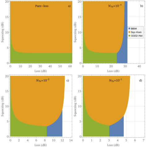
Figure 8: Regions where QKD protocols give the highest secret key rate greater than $K=10^{-10}$ based on the amount of squeezing $V_{\text{sq}}$ prepared by Alice for the squeezed-state protocol with homodyne detection. In the unshaded regions, $K$ is less than $10^{-10}$ for all protocols. Comparison of the squeezed-state protocol with homodyne detection in a pure-loss channel based on the amount of squeezing prepared by Alice. Above $9\text{ dB}$ of squeezing, the Sqz-Hom protocol performs better than GG02 and BB84 protocols.

References

- Hosseinidehaj et al. (2019) N. Hosseinidehaj, Z. Babar, R. Malaney, S. X. Ng, and L. Hanzo, IEEE Communications Surveys Tutorials 21, 881 (2019).
- Bennett and Brassard (2014) C. H. Bennett and G. Brassard, Theoretical Computer Science 560, 7 (2014), theoretical Aspects of Quantum Cryptography – celebrating 30 years of BB84.
- Su (2020) H.-Y. Su, Quantum Information Processing 19, 169 (2020).
- Ralph (1999) T. C. Ralph, Phys. Rev. A 61, 010303 (1999).
- Ralph (2000) T. C. Ralph, Phys. Rev. A 62, 062306 (2000).
- Hillery (2000) M. Hillery, Phys. Rev. A 61, 022309 (2000).
- Cerf et al. (2001) N. J. Cerf, M. Lévy, and G. V. Assche, Phys. Rev. A 63, 052311 (2001).
- Grosshans and Grangier (2002) F. Grosshans and P. Grangier, Phys. Rev. Lett. 88, 057902 (2002).
- Grosshans et al. (2003) F. Grosshans, G. Van Assche, J. Wenger, R. Brouri, N. J. Cerf, and P. Grangier, Nature 421, 238 (2003).
- Weedbrook et al. (2004) C. Weedbrook, A. M. Lance, W. P. Bowen, T. Symul, T. C. Ralph, and P. K. Lam, Phys. Rev. Lett. 93, 170504 (2004).
- Silberhorn et al. (2002) C. Silberhorn, T. C. Ralph, N. Lütkenhaus, and G. Leuchs, Phys. Rev. Lett. 89, 167901 (2002).
- Wang et al. (2019) X. Wang, S. Guo, P. Wang, W. Liu, and Y. Li, Opt. Express 27, 13372 (2019).
- Pirandola et al. (2020) S. Pirandola, U. L. Andersen, L. Banchi, M. Berta, D. Bunandar, R. Colbeck, D. Englund, T. Gehring, C. Lupo, C. Ottaviani, J. L. Pereira, M. Razavi, J. S. Shaari, M. Tomamichel, V. C. Usenko, G. Vallone, P. Villoresi, and P. Wallden, Adv. Opt. Photon. 12, 1012 (2020).
- Pirandola et al. (2015) S. Pirandola, C. Ottaviani, G. Spedalieri, C. Weedbrook, S. L. Braunstein, S. Lloyd, T. Gehring, C. S. Jacobsen, and U. L. Andersen, Nature Photonics 9, 397 (2015).
- Xu et al. (2015) F. Xu, M. Curty, B. Qi, L. Qian, and H.-K. Lo, Nature Photonics 9, 772 (2015).
- Lasota et al. (2017) M. Lasota, R. Filip, and V. C. Usenko, Phys. Rev. A 95, 062312 (2017).
- Diamanti et al. (2016) E. Diamanti, H.-K. Lo, B. Qi, and Z. Yuan, npj Quantum Information 2, 16025 (2016).
- Chen et al. (2021) Y.-A. Chen, Q. Zhang, T.-Y. Chen, W.-Q. Cai, S.-K. Liao, J. Zhang, K. Chen, J. Yin, J.-G. Ren, Z. Chen, S.-L. Han, Q. Yu, K. Liang, F. Zhou, X. Yuan, M.-S. Zhao, T.-Y. Wang, X. Jiang, L. Zhang, W.-Y. Liu, Y. Li, Q. Shen, Y. Cao, C.-Y. Lu, R. Shu, J.-Y. Wang, L. Li, N.-L. Liu, F. Xu, X.-B. Wang, C.-Z. Peng, and J.-W. Pan, Nature 589, 214 (2021).
- Shor and Preskill (2000) P. W. Shor and J. Preskill, Phys. Rev. Lett. 85, 441 (2000).
- Renner (2008) R. Renner, International Journal of Quantum Information 06, 1 (2008), https://doi.org/10.1142/S0219749908003256 .
- Murta et al. (2020) G. Murta, F. Rozpędek, J. Ribeiro, D. Elkouss, and S. Wehner, Phys. Rev. A 101, 062321 (2020).
- Wilde (2017) M. M. Wilde, Quantum Information Theory, 2nd ed. (Cambridge University Press, 2017).
- Renner et al. (2005) R. Renner, N. Gisin, and B. Kraus, Phys. Rev. A 72, 012332 (2005).
- Sańchez (2007) R. G.-P. Sańchez (2007).
- Wolf et al. (2006) M. M. Wolf, G. Giedke, and J. I. Cirac, Phys. Rev. Lett. 96, 080502 (2006).
- García-Patrón and Cerf (2006) R. García-Patrón and N. J. Cerf, Phys. Rev. Lett. 97, 190503 (2006).
- Navascués et al. (2006) M. Navascués, F. Grosshans, and A. Acín, Phys. Rev. Lett. 97, 190502 (2006).
- Laudenbach et al. (2018) F. Laudenbach, C. Pacher, C.-H. F. Fung, A. Poppe, M. Peev, B. Schrenk, M. Hentschel, P. Walther, and H. Hübel, Advanced Quantum Technologies 1, 1800011 (2018).
- García-Patrón and Cerf (2009) R. García-Patrón and N. J. Cerf, Phys. Rev. Lett. 102, 130501 (2009).
- Lami and Wilde (2022) L. Lami and M. M. Wilde, “Exact solution for the quantum and private capacities of bosonic dephasing channels,” (2022).
- Lamoureux et al. (2005) L.-P. Lamoureux, E. Brainis, N. J. Cerf, P. Emplit, M. Haelterman, and S. Massar, Phys. Rev. Lett. 94, 230501 (2005).
- Qi et al. (2015) B. Qi, P. Lougovski, R. Pooser, W. Grice, and M. Bobrek, Phys. Rev. X 5, 041009 (2015).
- Marie and Alléaume (2017) A. Marie and R. Alléaume, Phys. Rev. A 95, 012316 (2017).
- Tang et al. (2020) X. Tang, R. Kumar, S. Ren, A. Wonfor, R. Penty, and I. White, Optics Communications 471, 126034 (2020).
- Pirandola et al. (2017) S. Pirandola, R. Laurenza, C. Ottaviani, and L. Banchi, Nature Communications 8, 15043 (2017).
- Pirandola et al. (2009) S. Pirandola, R. García-Patrón, S. L. Braunstein, and S. Lloyd, Phys. Rev. Lett. 102, 050503 (2009).
- Vahlbruch et al. (2016) H. Vahlbruch, M. Mehmet, K. Danzmann, and R. Schnabel, Phys. Rev. Lett. 117, 110801 (2016).
- Pirandola et al. (2018) S. Pirandola, S. L. Braunstein, R. Laurenza, C. Ottaviani, T. P. W. Cope, G. Spedalieri, and L. Banchi, Quantum Science and Technology 3, 035009 (2018).
- Wang et al. (2018) T. Wang, P. Huang, Y. Zhou, W. Liu, H. Ma, S. Wang, and G. Zeng, Opt. Express 26, 2794 (2018).
- Wang et al. (2020) H. Wang, Y. Pi, W. Huang, Y. Li, Y. Shao, J. Yang, J. Liu, C. Zhang, Y. Zhang, and B. Xu, Opt. Express 28, 32882 (2020).
- Chin et al. (2021) H.-M. Chin, N. Jain, D. Zibar, U. L. Andersen, and T. Gehring, npj Quantum Information 7, 20 (2021).
- Hajomer et al. (2022) A. A. Hajomer, H. Mani, N. Jain, H.-M. Chin, U. L. Andersen, and T. Gehring, in European Conference on Optical Communication (ECOC) 2022 (Optica Publishing Group, 2022) p. Th1G.5.
- Zhang et al. (2020) Y. Zhang, Z. Chen, S. Pirandola, X. Wang, C. Zhou, B. Chu, Y. Zhao, B. Xu, S. Yu, and H. Guo, Phys. Rev. Lett. 125, 010502 (2020).
- Boaron et al. (2018) A. Boaron, G. Boso, D. Rusca, C. Vulliez, C. Autebert, M. Caloz, M. Perrenoud, G. Gras, F. Bussières, M.-J. Li, D. Nolan, A. Martin, and H. Zbinden, Phys. Rev. Lett. 121, 190502 (2018).
- Li et al. (2023) W. Li, L. Zhang, H. Tan, Y. Lu, S.-K. Liao, J. Huang, H. Li, Z. Wang, H.-K. Mao, B. Yan, Q. Li, Y. Liu, Q. Zhang, C.-Z. Peng, L. You, F. Xu, and J.-W. Pan, Nature Photonics (2023), 10.1038/s41566-023-01166-4.
- Caloz et al. (2018) M. Caloz, M. Perrenoud, C. Autebert, B. Korzh, M. Weiss, C. Schönenberger, R. J. Warburton, H. Zbinden, and F. Bussières, Applied Physics Letters 112 (2018), 10.1063/1.5010102, 061103, https://pubs.aip.org/aip/apl/article-pdf/doi/10.1063/1.5010102/13301241/061103_1_online.pdf .
- Zhou et al. (2021) C. Zhou, X. Wang, Z. Zhang, S. Yu, Z. Chen, and H. Guo, Science China Physics, Mechanics & Astronomy 64, 260311 (2021).
- Usenko (2018) V. C. Usenko, Phys. Rev. A 98, 032321 (2018).
- Derkach et al. (2020) I. Derkach, V. C. Usenko, and R. Filip, New Journal of Physics 22, 053006 (2020).
- Hosseinidehaj et al. (2022) N. Hosseinidehaj, M. S. Winnel, and T. C. Ralph, Phys. Rev. A 105, 032602 (2022).
- Madsen et al. (2012) L. S. Madsen, V. C. Usenko, M. Lassen, R. Filip, and U. L. Andersen, Nature Communications 3, 1083 (2012).
- Wang et al. (2021) Y. Wang, W. Zhang, R. Li, L. Tian, and Y. Zheng, Applied Physics Letters 118, 134001 (2021).
- Davis et al. (2018) N. Davis, M. E. Shirokov, and M. M. Wilde, Phys. Rev. A 97, 062310 (2018).
Acknowledgements
We wish to acknowledge Spyros Tserkis and Matthew Winnel for their valuable discussions. This research was supported by the Australian Research Council (ARC) under the Centre of Excellence for Quantum Computation and Communication Technology (Grant No. CE110001027).