Generalized Policy Improvement Algorithms
with Theoretically Supported Sample Reuse

Abstract

Data-driven, learning-based control methods offer the potential to improve operations in complex systems, and model-free deep reinforcement learning represents a popular approach to data-driven control. However, existing classes of algorithms present a trade-off between two important deployment requirements for real-world control: (i) practical performance guarantees and (ii) data efficiency. Off-policy algorithms make efficient use of data through sample reuse but lack theoretical guarantees, while on-policy algorithms guarantee approximate policy improvement throughout training but suffer from high sample complexity. In order to balance these competing goals, we develop a class of Generalized Policy Improvement algorithms that combines the policy improvement guarantees of on-policy methods with the efficiency of sample reuse. We demonstrate the benefits of this new class of algorithms through extensive experimental analysis on a variety of continuous control tasks from the DeepMind Control Suite.

Policy improvement, policy optimization, reinforcement learning, sample reuse.

1 Introduction

Model-free reinforcement learning (RL) represents a successful framework for data-driven control in systems with unknown or complex dynamics [1, 2], where a learning-based approach to control is necessary. Model-free deep RL algorithms have demonstrated impressive performance on a variety of simulated control tasks in recent years [3], and serve as fundamental building blocks in other RL approaches such as model-based [4, 5, 6], offline [7, 8, 9], and safe [10, 11, 12, 13, 14] control methods.

Despite this success, adoption of deep RL methods has remained limited for high-stakes real-world control, where stable performance is critical and data collection can be both expensive and time-consuming. In order to reliably deploy data-driven control methods in these real-world settings, we require algorithms that (i) provide practical guarantees on performance throughout training and (ii) make efficient use of data collected in the environment. Unfortunately, these represent competing goals in existing model-free deep RL methods.

Off-policy deep RL algorithms achieve data efficiency through the use of a replay buffer during training, which allows samples to be used for multiple policy updates. Typically, the replay buffer stores millions of samples, which enables state-of-the-art performance on popular benchmarks. However, this aggressive form of sample reuse can lead to high computation and memory requirements when combined with deep neural network policy representations and rich sensory data such as images. As a result, popular off-policy algorithms are not compatible with many resource-constrained control settings that require real-time, on-device learning [15, 16, 17, 18, 19]. Most importantly, the characteristics of the replay buffer are treated as hyperparameters, resulting in sample reuse that lacks practical performance guarantees. These drawbacks prevent off-policy deep RL from being a broadly applicable solution for real-world control, and other data-driven methods are required.

An alternative class of deep RL algorithms only uses data collected under the current policy to perform updates (i.e., on-policy). By doing so, these on-policy methods guarantee approximate policy improvement throughout training, which is often a prerequisite for the deployment of data-driven control in real-world systems. In addition, on-policy approaches require significantly less computation and memory compared to off-policy algorithms [17], making them a viable option in settings that preclude the use of large replay buffers. For these reasons, we consider on-policy algorithms as our starting point in this work. However, the requirement of on-policy data results in high sample complexity and slow learning, which limits the effectiveness of these algorithms in practice.

Given our goal of reliable and efficient training, in this work we combine the policy improvement benefits of on-policy methods with the efficiency of sample reuse. Building upon prior work we reported in [20], we propose a new class of algorithms that we call Generalized Policy Improvement (GPI) algorithms. Our GPI algorithms extend on-policy methods to incorporate sample reuse, without sacrificing their approximate policy improvement guarantees during training. As a result, our GPI algorithms are similar to on-policy algorithms, but allow for the reuse of samples from all recent policies. This is in contrast to the aggressive, resource-intensive sample reuse in off-policy methods that lacks practical performance guarantees.

Our main contributions are as follows:

1. We establish a Generalized Policy Improvement lower bound in Section 4 that is compatible with the use of data from past policies.

2. Using this lower bound, in Section 5 we demonstrate how to optimally reuse data from all recent policies. Specifically, our theoretically supported sample reuse improves the trade-off between batch size and policy update size throughout training compared to on-policy methods, while retaining the same approximate policy improvement guarantees.

3. We propose a class of Generalized Policy Improvement algorithms in Section 6 that combines popular on-policy methods with theoretically supported sample reuse. In particular, we develop generalized versions of three popular on-policy algorithms: Proximal Policy Optimization (PPO) [21], Trust Region Policy Optimization (TRPO) [22], and On-Policy Maximum a Posteriori Policy Optimization (VMPO) [23].

4. In Section 7, we demonstrate the practical benefits of our algorithms through extensive experimental analysis on 28 continuous control benchmarking tasks from the DeepMind Control Suite [24].

This paper extends our work in [20], where we first introduced the Generalized Policy Improvement lower bound to motivate a generalized version of PPO. Compared to [20], which focused on a single algorithm, in this paper we propose a unified algorithmic framework that we use to improve the efficiency of many popular on-policy methods. We also expand our analysis on theoretically supported sample reuse and conduct a thorough experimental investigation across a broad range of new tasks, providing additional insights into the trade-offs associated with our GPI algorithms and the settings where they are most beneficial. Proofs of all results presented throughout the paper can be found in the Appendix.

2 Related Work

2.1 On-Policy Policy Improvement Methods

Our work focuses on policy improvement methods, an algorithmic framework that was first introduced by [25] in Conservative Policy Iteration (CPI). CPI guarantees policy improvement by considering a mixture between the current and greedy policies at every update. The policy improvement bounds proposed by [25] were later refined by [22] and [10], making them compatible with the deep RL setting. These advances motivated the development of many popular on-policy policy improvement methods, including TRPO [22] and PPO [21]. The strong empirical performance of TRPO and PPO has been studied in detail [26, 27, 28]. In addition, these algorithms have served as the foundation for many on-policy extensions. The work in [10] extended TRPO to the constrained setting, [29] proposed a robust version of TRPO from limited data, and [30, 31, 32] considered modifications to the clipping mechanism in PPO. Given the popularity of TRPO and PPO, we consider both of these algorithms when developing our family of GPI algorithms.

In recent years, on-policy methods have also considered non-parametric target policies obtained by solving policy optimization problems similar to those used in TRPO and PPO. These target policies are then projected back onto the space of parameterized policies. The framework proposed in [33] considered a variety of non-parametric target policies, while [23] focused on the target policy induced by a reverse Kullback-Leibler (KL) divergence constraint in their algorithm VMPO. Note that VMPO is motivated by applying the expectation-maximization framework from [34] to the on-policy setting, but its practical trust region implementation can also be interpreted from a policy improvement perspective. In addition to generalized versions of TRPO and PPO, we also propose a generalized version of VMPO as a representative instance of policy improvement algorithms based on non-parametric target policies.

2.2 Sample Efficiency with Off-Policy Data

The main drawback of on-policy policy improvement algorithms is their requirement of on-policy data, which can lead to slow and inefficient learning. Popular off-policy algorithms [35, 36, 37, 34] address this issue by storing data in a replay buffer and reusing samples for multiple policy updates. These algorithms do not explicitly control the bias introduced by off-policy data, and as a result do not provide practical policy improvement guarantees. Typically, these algorithms employ aggressive, resource-intensive sample reuse through the use of a large replay buffer, and they rely on careful hyperparameter tuning along with implementation tricks such as target networks and double Q-learning to avoid instability.

Methods have been proposed to address the bias introduced by off-policy data. One line of work combines on-policy and off-policy updates to address this concern [38, 39, 40, 41, 42, 43], and some of these methods consider regularization terms related to our approach. The theoretical analysis in [40] demonstrated that the bias of off-policy data is related to the KL divergence between the current policy and the data-generating policy, and [41] considered a trust region closely related to this result. The update in [42] applied a related KL divergence penalty term, while [43] approximated this KL divergence by applying a trust region around a target policy. These approaches are similar to the generalized KL divergence trust regions that we consider in our Generalized TRPO and VMPO algorithms.

Other approaches have modified the use of the replay buffer to control the bias from off-policy data. The updates in [44] ignored samples from the replay buffer whose actions were not likely under the current policy, and [45] considered a sampling scheme that emphasized more recent experience in the replay buffer. The theoretically supported sample reuse that we consider in our GPI algorithms can be viewed as restricting the size of the replay buffer to only contain recent policies, as well as applying a non-uniform weighting to the samples.

3 Preliminaries

3.1 Reinforcement Learning Framework

We represent the sequential decision making problem as an infinite-horizon, discounted Markov decision process (MDP) defined by the tuple $(\mathcal{S},\mathcal{A},p,r,\rho_{0},\gamma)$, where $\mathcal{S}$ is the set of states, $\mathcal{A}$ is the set of actions, $p:\mathcal{S}\times\mathcal{A}\rightarrow P(\mathcal{S})$ is the transition probability function where $P(\mathcal{S})$ represents the space of probability measures over $\mathcal{S}$, $r:\mathcal{S}\times\mathcal{A}\rightarrow\mathbb{R}$ is the reward function, $\rho_{0}\in P(\mathcal{S})$ is the initial state distribution, and $\gamma$ is the discount rate.

We model the agent’s decisions as a stationary policy $\pi:\mathcal{S}\rightarrow P(\mathcal{A})$, which outputs a distribution of actions at every state. Our goal is to find a policy $\pi$ that maximizes the expected total discounted return $J(\pi)=\mathop{\mathbb{E}}_{\tau\sim\pi}\left[\sum_{t=0}^{\infty}\gamma^{t}r(s_{t},a_{t})\right]$, where $\tau\sim\pi$ represents a trajectory sampled according to $s_{0}\sim\rho_{0}$, $a_{t}\sim\pi(\,\cdot\mid s_{t})$, and $s_{t+1}\sim p(\,\cdot\mid s_{t},a_{t})$. A policy $\pi$ also induces a normalized discounted state visitation distribution $d^{\pi}$, where $d^{\pi}(s)=(1-\gamma)\sum_{t=0}^{\infty}\gamma^{t}\mathbb{P}(s_{t}=s\mid\rho_{0},\pi,p)$. We write the corresponding normalized discounted state-action visitation distribution as $d^{\pi}(s,a)=d^{\pi}(s)\pi(a\mid s)$, where we make it clear from the context whether $d^{\pi}$ refers to a distribution over states or state-action pairs.

We denote the state value function of $\pi$ as $V^{\pi}(s)=\mathop{\mathbb{E}}_{\tau\sim\pi}\left[\sum_{t=0}^{\infty}\gamma^{t}r(s_{t},a_{t})\mid s_{0}=s\right]$, the state-action value function as $Q^{\pi}(s,a)=\mathop{\mathbb{E}}_{\tau\sim\pi}\left[\sum_{t=0}^{\infty}\gamma^{t}r(s_{t},a_{t})\mid s_{0}=s,a_{0}=a\right]$, and the advantage function as $A^{\pi}(s,a)=Q^{\pi}(s,a)-V^{\pi}(s)$.

3.2 On-Policy Policy Improvement Lower Bound

Many popular on-policy algorithms can be interpreted as approximately maximizing the following policy improvement lower bound, which was first developed by [25] and later refined by [22] and [10].

Lemma 1 (From [10])

Consider any policy $\pi$ and a current policy $\pi_{k}$. Then,

$$J(\pi)-J(\pi_{k})\geq\frac{1}{1-\gamma}\mathop{\mathbb{E}}_{(s,a)\sim d^{\pi_{k}}}\left[\frac{\pi(a\mid s)}{\pi_{k}(a\mid s)}A^{\pi_{k}}(s,a)\right]\\ -\frac{2\gamma C^{\pi,\pi_{k}}}{(1-\gamma)^{2}}\mathop{\mathbb{E}}_{s\sim d^{\pi_{k}}}\left[\operatorname{TV}\left(\pi,\pi_{k}\right)(s)\right],$$ (1)

where $C^{\pi,\pi_{k}}=\max_{s\in\mathcal{S}}\left|\mathop{\mathbb{E}}_{a\sim\pi(\,\cdot\,\mid s)}\left[A^{\pi_{k}}(s,a)\right]\right|$ and $\operatorname{TV}\left(\pi,\pi_{k}\right)(s)$ represents the total variation (TV) distance between the distributions $\pi(\,\cdot\mid s)$ and $\pi_{k}(\,\cdot\mid s)$.

We refer to the first term on the right-hand side of (1) as the surrogate objective and the second term as the penalty term. There are two important items to note about the policy improvement lower bound in Lemma 1. First, we can guarantee monotonic policy improvement at every update by maximizing this lower bound, leading to reliable performance throughout training. Second, the expectations that appear in the surrogate objective and penalty term can be estimated using samples collected under the current policy $\pi_{k}$. Therefore, this bound motivates algorithms that are practical to implement, but may result in slow learning due to their requirement of on-policy data.

3.3 On-Policy Policy Improvement Algorithms

Rather than directly maximize the lower bound in Lemma 1, on-policy policy improvement algorithms typically maximize the surrogate objective while bounding the risk of each policy update via a constraint on the penalty term. This leads to updates with the following form.

Definition 2

For a given choice of trust region parameter $\epsilon>0$, the on-policy trust region update has the form

$$\begin{split}\pi_{k+1}=\arg\max_{\pi}\,\,&\mathop{\mathbb{E}}_{(s,a)\sim d^{\pi_{k}}}\left[\frac{\pi(a\mid s)}{\pi_{k}(a\mid s)}A^{\pi_{k}}(s,a)\right]\\ \textnormal{s.t.}\,\,&\mathop{\mathbb{E}}_{s\sim d^{\pi_{k}}}\left[\operatorname{TV}\left(\pi,\pi_{k}\right)(s)\right]\leq\frac{\epsilon}{2}.\end{split}$$ (2)

The trust region in (2) bounds the magnitude of the penalty term in (1), limiting the worst-case performance decline at every update. Therefore, we say that on-policy algorithms based on the trust region update in Definition 2 deliver approximate policy improvement guarantees. In addition, practical deep RL implementations of this update introduce additional approximations through the use of sample-based estimates.

The difference between popular on-policy algorithms is primarily due to how they approximately solve the optimization problem in Definition 2. PPO applies a TV distance trust region via a clipping mechanism, while TRPO and VMPO instead consider forward and reverse KL divergence trust regions, respectively. These related trust regions guarantee that the TV distance trust region in (2) is satisfied, as shown in the following result.

Lemma 3

Consider a current policy $\pi_{k}$, and any policy $\pi$ that satisfies

$$\mathop{\mathbb{E}}_{s\sim d^{\pi_{k}}}\left[\operatorname{KL}\left(\pi_{k}\|\pi\right)(s)\right]\leq\delta,$$ (3)

or

$$\mathop{\mathbb{E}}_{s\sim d^{\pi_{k}}}\left[\operatorname{KL}\left(\pi\|\pi_{k}\right)(s)\right]\leq\delta,$$ (4)

where $\operatorname{KL}\left(\pi_{k}\|\pi\right)(s)$ and $\operatorname{KL}\left(\pi\|\pi_{k}\right)(s)$ represent the forward and reverse Kullback-Leibler (KL) divergence of the distribution $\pi(\,\cdot\mid s)$ from the distribution $\pi_{k}(\,\cdot\mid s)$, respectively, and $\delta=\nicefrac{{\epsilon^{2}}}{{2}}$. Then, $\pi$ also satisfies the TV distance trust region in (2).

The high-level framework of on-policy policy improvement algorithms is described in Algorithm 1.

Input: initial policy $\pi_{0}$; TV distance trust region parameter $\epsilon$; batch size $N$.

for $k=0,1,2,\ldots$ do

      Collect $N$ samples with $\pi_{k}$. Use these $N$ samples to approximate the expectations in Definition 2. Update policy by approximately solving the optimization problem in Definition 2. Implementation varies by algorithm.

      end for

Algorithm 1 On-Policy Policy Improvement

4 Generalized Policy Improvement Lower Bound

The goal of our work is to improve the efficiency of on-policy algorithms through sample reuse, without sacrificing their approximate policy improvement guarantees. In order to relax the on-policy requirement of the expectations that appear in Lemma 1, our key insight is that we can construct a similar policy improvement bound with expectations that depend on any reference policy.

Lemma 4

Consider any policy $\pi$ and a reference policy $\pi_{\textnormal{ref}}$. Then,

$$J(\pi)-J(\pi_{k})\geq\frac{1}{1-\gamma}\mathop{\mathbb{E}}_{(s,a)\sim d^{\pi_{\textnormal{ref}}}}\left[\frac{\pi(a\mid s)}{\pi_{\textnormal{ref}}(a\mid s)}A^{\pi_{k}}(s,a)\right]\\ -\frac{2\gamma C^{\pi,\pi_{k}}}{(1-\gamma)^{2}}\mathop{\mathbb{E}}_{s\sim d^{\pi_{\textnormal{ref}}}}\left[\operatorname{TV}\left(\pi,\pi_{\textnormal{ref}}\right)(s)\right],$$

where $C^{\pi,\pi_{k}}$ is defined as in Lemma 1.

By considering our prior policies as reference policies, we can use Lemma 4 to develop a Generalized Policy Improvement lower bound that is compatible with sample reuse.

Theorem 5

Consider any policy $\pi$ and prior policies $\pi_{k-i}$, $i=0,1,2,\ldots$. Let $\nu$ be any choice of mixture distribution over prior policies, where $0\leq\nu_{i}\leq 1$ is the probability of using $\pi_{k-i}$ as the reference policy, $\sum_{i}\nu_{i}=1$, and $\mathop{\mathbb{E}}_{i\sim\nu}\left[\,\cdot\,\right]$ represents an expectation determined by this mixture distribution. Then, we have that

$$J(\pi)-J(\pi_{k})\\ \geq\frac{1}{1-\gamma}\mathop{\mathbb{E}}_{i\sim\nu}\left[\mathop{\mathbb{E}}_{(s,a)\sim d^{\pi_{k-i}}}\left[\frac{\pi(a\mid s)}{\pi_{k-i}(a\mid s)}A^{\pi_{k}}(s,a)\right]\right]\\ -\frac{2\gamma C^{\pi,\pi_{k}}}{(1-\gamma)^{2}}\mathop{\mathbb{E}}_{i\sim\nu}\left[\mathop{\mathbb{E}}_{s\sim d^{\pi_{k-i}}}\left[\operatorname{TV}\left(\pi,\pi_{k-i}\right)(s)\right]\right],$$ (5)

where $C^{\pi,\pi_{k}}$ is defined as in Lemma 1.

The expectations that appear in our Generalized Policy Improvement lower bound can be estimated using a mixture of samples collected under prior policies, so Theorem 5 provides insight into how we can reuse samples while still providing guarantees on performance throughout training. The cost of sample reuse is that the penalty term now depends on the expected TV distance between the new policy and our prior policies, rather than the current policy. Otherwise, our lower bound remains largely unchanged compared to the on-policy case. In fact, we recover the on-policy lower bound when $\nu$ is chosen to place all weight on the current policy, so Lemma 1 is a special case of Theorem 5.

Because the structure of our generalized lower bound remains the same as the on-policy lower bound, we can use the same techniques to motivate practical policy improvement algorithms. Just as the on-policy lower bound motivated the policy update in Definition 2, we can use Theorem 5 to motivate a generalized policy update of the form

$$\begin{split}\pi_{k+1}=\arg\max_{\pi}\,\,&\mathop{\mathbb{E}}_{i\sim\nu}\left[\mathop{\mathbb{E}}_{(s,a)\sim d^{\pi_{k-i}}}\left[\frac{\pi(a\mid s)}{\pi_{k-i}(a\mid s)}A^{\pi_{k}}(s,a)\right]\right]\\ \textnormal{s.t.}\,\,&\mathop{\mathbb{E}}_{i\sim\nu}\left[\mathop{\mathbb{E}}_{s\sim d^{\pi_{k-i}}}\left[\operatorname{TV}\left(\pi,\pi_{k-i}\right)(s)\right]\right]\leq\frac{\epsilon}{2},\end{split}$$ (6)

where $\epsilon$ represents the same trust region parameter used in the on-policy case. By the triangle inequality of TV distance, we have that

$$\mathop{\mathbb{E}}_{i\sim\nu}\left[\mathop{\mathbb{E}}_{s\sim d^{\pi_{k-i}}}\left[\operatorname{TV}\left(\pi,\pi_{k-i}\right)(s)\right]\right]\\ \leq\mathop{\mathbb{E}}_{i\sim\nu}\left[\mathop{\mathbb{E}}_{s\sim d^{\pi_{k-i}}}\left[\operatorname{TV}\left(\pi,\pi_{k}\right)(s)\right]\right]\\ +\mathop{\mathbb{E}}_{i\sim\nu}\left[\mathop{\mathbb{E}}_{s\sim d^{\pi_{k-i}}}\left[\operatorname{TV}\left(\pi_{k},\pi_{k-i}\right)(s)\right]\right],$$ (7)

where the first term on the right-hand side is the expected one-step TV distance and the second term does not depend on $\pi$. Therefore, we can satisfy the trust region in (6) by controlling the expected one-step TV distance, which is often easier to work with in practice. For an appropriate choice of $\epsilon_{\textnormal{GPI}}$, this leads to the following policy update.

Definition 6

For a given choice of trust region parameter $\epsilon_{\textnormal{GPI}}>0$, the generalized trust region update has the form

$$\begin{split}\pi_{k+1}=\arg\max_{\pi}\,\,&\mathop{\mathbb{E}}_{i\sim\nu}\left[\mathop{\mathbb{E}}_{(s,a)\sim d^{\pi_{k-i}}}\left[\frac{\pi(a\mid s)}{\pi_{k-i}(a\mid s)}A^{\pi_{k}}(s,a)\right]\right]\\ \textnormal{s.t.}\,\,&\mathop{\mathbb{E}}_{i\sim\nu}\left[\mathop{\mathbb{E}}_{s\sim d^{\pi_{k-i}}}\left[\operatorname{TV}\left(\pi,\pi_{k}\right)(s)\right]\right]\leq\frac{\epsilon_{\textnormal{GPI}}}{2}.\end{split}$$ (8)

Similar to the on-policy trust region update in Definition 2, the generalized trust region update also provides approximate policy improvement guarantees due to its connection to the Generalized Policy Improvement lower bound in Theorem 5. In order to deliver these approximate policy improvement guarantees, the generalized update still depends on the advantage function with respect to the current policy $\pi_{k}$, which must be approximated using off-policy estimation techniques in practice.

As in the on-policy case, we can also satisfy the one-step TV distance trust region in (8) by instead considering related forward or reverse KL divergence trust regions.

Lemma 7

Consider prior policies $\pi_{k-i}$, $i=0,1,2,\ldots$, and any policy $\pi$ that satisfies

$$\mathop{\mathbb{E}}_{i\sim\nu}\left[\mathop{\mathbb{E}}_{s\sim d^{\pi_{k-i}}}\left[\operatorname{KL}\left(\pi_{k}\|\pi\right)(s)\right]\right]\leq\delta_{\textnormal{GPI}},$$ (9)

or

$$\mathop{\mathbb{E}}_{i\sim\nu}\left[\mathop{\mathbb{E}}_{s\sim d^{\pi_{k-i}}}\left[\operatorname{KL}\left(\pi\|\pi_{k}\right)(s)\right]\right]\leq\delta_{\textnormal{GPI}},$$ (10)

where $\delta_{\textnormal{GPI}}=\nicefrac{{\epsilon_{\textnormal{GPI}}^{2}}}{{2}}$. Then, $\pi$ also satisfies the TV distance trust region in (8).

Next, we describe how to select the generalized trust region parameter $\epsilon_{\textnormal{GPI}}$ and mixture distribution $\nu$ over prior policies in order to provide guarantees on the risk of every policy update while optimizing key quantities of interest. Principled choices of $\epsilon_{\textnormal{GPI}}$ and $\nu$ result in theoretically supported sample reuse.

5 Theoretically Supported Sample Reuse

5.1 Generalized Trust Region Parameter

Note that our Generalized Policy Improvement lower bound is valid for any mixture distribution $\nu$ over prior policies, and the magnitude of the penalty term depends on the choice of $\nu$. Therefore, we first determine how to select $\epsilon_{\textnormal{GPI}}$ for a given mixture distribution $\nu$ in order to provide the same performance guarantees as the on-policy setting.

From (7), we see that the generalized update in Definition 6 satisfies the trust region in (6) for any $\epsilon_{\textnormal{GPI}}$ such that

$$\frac{\epsilon_{\textnormal{GPI}}}{2}\leq\frac{\epsilon}{2}-\mathop{\mathbb{E}}_{i\sim\nu}\left[\mathop{\mathbb{E}}_{s\sim d^{\pi_{k-i}}}\left[\operatorname{TV}\left(\pi_{k},\pi_{k-i}\right)(s)\right]\right].$$ (11)

While the adaptive choice of $\epsilon_{\textnormal{GPI}}$ given by (11) will successfully control the magnitude of the penalty term in the Generalized Policy Improvement lower bound, it only indirectly provides insight into how $\epsilon_{\textnormal{GPI}}$ depends on the choice of $\nu$. In order to establish a more direct connection between $\epsilon_{\textnormal{GPI}}$ and $\nu$, we consider a slightly stronger trust region assumption.

Theorem 8

Assume that the expected one-step TV distance under each state visitation distribution $d^{\pi_{k-i}}$ is bounded by $\nicefrac{{\epsilon_{\textnormal{GPI}}}}{{2}}$ at every update, where

$$\epsilon_{\textnormal{GPI}}=\frac{\epsilon}{\mathop{\mathbb{E}}_{i\sim\nu}\left[\,i+1\,\right]}.$$

Then, the magnitude of the generalized penalty term is no greater than the magnitude of the on-policy penalty term under the on-policy update in Definition 2.

Although the generalized update in Definition 6 does not directly imply the trust region assumption in Theorem 8, practical implementations based on clipping mechanisms or backtracking line searches can ensure that this assumption holds. In practice, the choice of $\epsilon_{\textnormal{GPI}}$ determined by Theorem 8 successfully controls the magnitude of the generalized penalty term, and tends to be conservative compared to (11) because it is based on applying the triangle inequality between every prior policy.

The form of $\epsilon_{\textnormal{GPI}}$ in Theorem 8 clearly demonstrates the trade-off of sample reuse. As we reuse older data, we must consider smaller one-step trust regions at every policy update in order to guarantee the same level of risk.

5.2 Mixture Distribution

Despite the need for smaller one-step trust regions at every policy update, we can show that our generalized policy update improves key quantities of interest when the mixture distribution $\nu$ is chosen in a principled manner. Note that $\nu_{i}>0$ indicates that data from $\pi_{k-i}$ will be used during updates, so the choice of $\nu$ determines how many prior policies to consider in addition to how to weight their contributions.

In this section, we show it is possible to select $\nu$ in a way that improves both the effective sample size and total TV distance update size throughout training compared to the on-policy baseline. It is common to consider auxiliary metrics to inform sampling schemes [46, 47], and these represent two important quantities in policy optimization. A larger effective sample size results in more accurate estimates of the expectations that we must approximate in policy updates, and leads to a more diverse batch of data which can be useful when reward signals are sparse [48]. A larger total TV distance update size allows for more aggressive exploitation of the available information, which can lead to faster learning throughout training. Although optimizing these metrics does not guarantee improved performance compared to on-policy algorithms, we see in Section 7 that experimentally this is often the case.

We write the on-policy sample size as $N=Bn$, where $B$ is a positive integer and $n$ represents the smallest possible batch size (for example, the length of one full trajectory). On-policy policy improvement algorithms update the policy according to Definition 2 after every $N$ samples collected, where the expectations are approximated using empirical averages calculated using these $N$ samples.

For the generalized case, we can combine data across several prior policies to construct the batch used to calculate the generalized policy update in Definition 6. Therefore, sample reuse allows us to make policy updates after every $n$ samples collected. The resulting effective sample size used for generalized policy updates is given by

$$f_{\textnormal{ESS}}(\nu)=\frac{n}{\sum_{i}\nu_{i}^{2}},$$

where $\nu_{i}$, $i=0,1,2,\ldots$, represents the weighting for data collected under $\pi_{k-i}$. We consider the effective sample size to account for the increased variance due to non-uniform weights [49]. For the case of uniform weights over the last $M$ policies, $f_{\textnormal{ESS}}(\nu)$ reduces to the standard sample size definition of $Mn$.

Because we calculate generalized policy updates after every $n$ samples collected, we are able to make $B$ times as many updates as the on-policy case. The total TV distance update size for every $N$ samples collected in the generalized case is given by

$$f_{\textnormal{TV}}(\nu)=B\cdot\frac{\epsilon_{\textnormal{GPI}}}{2}=\frac{B}{\sum_{i}\nu_{i}\left(i+1\right)}\cdot\frac{\epsilon}{2},$$

compared to $\nicefrac{{\epsilon}}{{2}}$ in on-policy algorithms.

Using the following result, we select $\nu$ to optimize $f_{\textnormal{ESS}}(\nu)$ and $f_{\textnormal{TV}}(\nu)$ relative to the on-policy case.

Theorem 9

Fix the trade-off parameter $\kappa\in[0,1]$, and select the mixture distribution $\nu$ according to the convex optimization problem

$$\begin{split}\nu^{*}(\kappa)=\arg\min_{\nu}\,\,&\kappa\cdot\frac{\sum_{i}\nu_{i}^{2}}{c_{\textnormal{ESS}}}+(1-\kappa)\cdot\frac{\sum_{i}\nu_{i}\left(i+1\right)}{c_{\textnormal{TV}}}\\ \textnormal{s.t.}\,\,&\sum_{i}\nu_{i}^{2}\leq\frac{1}{B},\quad\sum_{i}\nu_{i}\left(i+1\right)\leq B,\\ &\sum_{i}\nu_{i}=1,\quad\nu_{i}\geq 0,\,i=0,1,2,\ldots,\end{split}$$ (12)

where $c_{\textnormal{ESS}},c_{\textnormal{TV}}\geq 0$ are scaling coefficients. Then, the effective sample size and total TV distance update size of our GPI algorithms are at least as large as the corresponding quantities in the on-policy baseline.

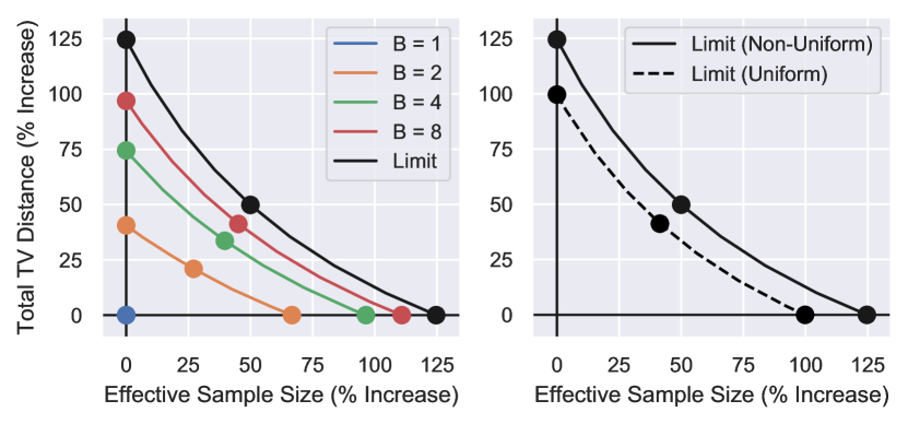
Figure 1: Benefit of GPI update compared to on-policy case. Represents percent increases in effective sample size and total TV distance update size for all possible values of $\kappa\in[0,1]$. Markers indicate $\kappa=0.0,0.5,1.0$. Left: Comparison across several values of $B$. Right: Comparison of non-uniform and uniform weights for large $B$.

We see the benefits of using the optimal mixture distribution from Theorem 9 in the left-hand side of Fig. 1. As $B$ becomes larger, the benefit of our generalized approach increases. A large value of $B$ indicates the need for batches that contain many sample trajectories, which may occur in highly stochastic environments or tasks with sparse rewards. In this case, we can improve the effective sample size or total TV distance update size by up to 125% compared to on-policy methods, without sacrificing performance with respect to the other. In the right-hand side of Fig. 1, we see that we can still achieve up to a 100% improvement in these metrics through sample reuse with uniform weights over prior policies. Therefore, the main benefit of optimizing $\nu$ comes from determining the appropriate number of prior policies to consider, with non-uniform weights offering additional improvements. Together, Theorem 8 and Theorem 9 provide theoretical support for the sample reuse we consider in this work.

In the continuous control benchmarking tasks we consider in Section 7, the default on-policy batch size used in the literature represents a low value of $B=2$. Because these environments have deterministic dynamics, some of these tasks may require only a small number of trajectories per batch to inform policy updates. Even in this case, we can improve the effective sample size by up to 67% or total TV distance update size by up to 41% compared to on-policy methods, without sacrificing performance with respect to the other. The optimal mixture distributions for $B=2$ are shown in Fig. 2 for three choices of trade-off parameter $\kappa$. When $B=2$, our theoretically supported sample reuse suggests using data from the prior three or four policies.

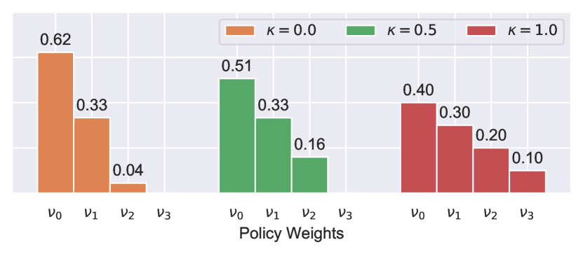
Figure 2: Optimal mixture distributions for $B=2$ and $\kappa=0.0,0.5,1.0$.

6 Generalized Policy Improvement Algorithms

The theory that we have developed can be used to construct generalized versions of on-policy algorithms with theoretically supported sample reuse. We refer to this class of algorithms as Generalized Policy Improvement (GPI) algorithms. The high-level framework for these algorithms is shown in Algorithm 2. By using the optimal mixture distribution from Theorem 9, GPI algorithms only require modest increases in memory and computation compared to on-policy algorithms. In addition, due to their use of one-step trust regions, GPI algorithms only need access to the current policy and value function in order to compute updates. As a result, deep RL implementations do not require storage of any additional neural networks compared to on-policy algorithms.

In this section, we provide details on three algorithms from this class: Generalized PPO (GePPO), Generalized TRPO (GeTRPO), and Generalized VMPO (GeVMPO). See the Appendix for additional implementation details.

Input: initial policy $\pi_{0}$; TV distance trust region parameter $\epsilon$; on-policy batch size $N=Bn$, where $n$ represents minimum batch size; trade-off parameter $\kappa$.

Calculate mixture distribution $\nu$ using Theorem 9, and let $M$ be the number of prior policies with non-zero weighting. Calculate generalized trust region parameter $\epsilon_{\textnormal{GPI}}$ using Theorem 8. for $k=0,1,2,\ldots$ do

      Collect $n$ samples with $\pi_{k}$. Use $n$ samples from each of $\pi_{k-i}$, $i=0,\ldots,M-1$, to approximate the expectations in Definition 6. Update policy by approximately solving the optimization problem in Definition 6. Implementation varies by algorithm.

      end for

Algorithm 2 Generalized Policy Improvement

6.1 Generalized PPO

PPO approximates the on-policy trust region update in Definition 2 using the policy update

$$\pi_{k+1}=\arg\max_{\pi}\mathop{\mathbb{E}}_{(s,a)\sim d^{\pi_{k}}}\left[\min\left(\frac{\pi(a\mid s)}{\pi_{k}(a\mid s)}A^{\pi_{k}}(s,a),\right.\right.\\ \left.\left.\operatorname{clip}\left(\frac{\pi(a\mid s)}{\pi_{k}(a\mid s)},1-\epsilon,1+\epsilon\right)A^{\pi_{k}}(s,a)\right)\right],$$ (13)

where $\operatorname{clip}(x,l,u)=\min(\max(x,l),u)$ and the maximization is implemented using minibatch stochastic gradient ascent. The policy update in (13) approximately maximizes a lower bound on the on-policy surrogate objective, while also heuristically enforcing

$$\left|\frac{\pi(a\mid s)}{\pi_{k}(a\mid s)}-1\right|\leq\epsilon$$

at every state-action pair through the use of the clipping mechanism in the second term. The clipping mechanism accomplishes this by removing any incentive for the probability ratio to deviate more than $\epsilon$ from its starting point during every policy update. Therefore, the clipping mechanism heuristically enforces the TV distance trust region in (2), as shown in the following result.

Lemma 10

Assume that the support of $\pi$ is contained within the support of $\pi_{k}$ at every state. Then, the TV distance trust region in (2) can be written as

$$\mathop{\mathbb{E}}_{s\sim d^{\pi_{k}}}\left[\operatorname{TV}\left(\pi,\pi_{k}\right)(s)\right]=\frac{1}{2}\mathop{\mathbb{E}}_{(s,a)\sim d^{\pi_{k}}}\left[\,\left|\frac{\pi(a\mid s)}{\pi_{k}(a\mid s)}-1\right|\,\right].$$

Note that the assumption in Lemma 10 is satisfied by popular policy representations such as a Gaussian policy.

In order to develop a generalized version of PPO that approximates the generalized trust region update in Definition 6, we desire a policy update that approximately maximizes a lower bound on the generalized surrogate objective while also heuristically enforcing the generalized trust region via a clipping mechanism. In order to determine the appropriate clipping mechanism, we can write the generalized TV distance trust region in (8) as the expectation of a probability ratio deviation just as we did in the on-policy case.

Lemma 11

Assume that the support of $\pi$ is contained within the support of $\pi_{k-i}$, $i=0,1,2,\ldots$, at every state. Then, the TV distance trust region in (8) can be written as

$$\mathop{\mathbb{E}}_{i\sim\nu}\left[\mathop{\mathbb{E}}_{s\sim d^{\pi_{k-i}}}\left[\operatorname{TV}\left(\pi,\pi_{k}\right)(s)\right]\right]\\ =\frac{1}{2}\mathop{\mathbb{E}}_{i\sim\nu}\left[\mathop{\mathbb{E}}_{(s,a)\sim d^{\pi_{k-i}}}\left[\,\left|\frac{\pi(a\mid s)}{\pi_{k-i}(a\mid s)}-\frac{\pi_{k}(a\mid s)}{\pi_{k-i}(a\mid s)}\right|\,\right]\right].$$

Therefore, Lemma 11 suggests the need for a clipping mechanism that heuristically enforces

$$\left|\frac{\pi(a\mid s)}{\pi_{k-i}(a\mid s)}-\frac{\pi_{k}(a\mid s)}{\pi_{k-i}(a\mid s)}\right|\leq\epsilon_{\textnormal{GPI}},$$

i.e., removes the incentive for the probability ratio to deviate more than $\epsilon_{\textnormal{GPI}}$ from its starting point of $\nicefrac{{\pi_{k}(a\mid s)}}{{\pi_{k-i}(a\mid s)}}$. By applying such a generalized clipping mechanism and considering a lower bound on the generalized surrogate objective, we arrive at the Generalized PPO (GePPO) update

$$\pi_{k+1}=\arg\max_{\pi}\mathop{\mathbb{E}}_{i\sim\nu}\Bigg{[}\mathop{\mathbb{E}}_{(s,a)\sim d^{\pi_{k-i}}}\bigg{[}\\ \min\bigg{(}\frac{\pi(a\mid s)}{\pi_{k-i}(a\mid s)}A^{\pi_{k}}(s,a),\operatorname{clip}\bigg{(}\frac{\pi(a\mid s)}{\pi_{k-i}(a\mid s)},\,\\ \frac{\pi_{k}(a\mid s)}{\pi_{k-i}(a\mid s)}-\epsilon_{\textnormal{GPI}},\,\frac{\pi_{k}(a\mid s)}{\pi_{k-i}(a\mid s)}+\epsilon_{\textnormal{GPI}}\bigg{)}A^{\pi_{k}}(s,a)\bigg{)}\bigg{]}\Bigg{]}.$$ (14)

6.2 Generalized TRPO

TRPO approximates the on-policy update in Definition 2 by instead applying the forward KL divergence trust region in (3). Therefore, TRPO considers the policy update

$$\begin{split}\pi_{k+1}=\arg\max_{\pi}\,\,&\mathop{\mathbb{E}}_{(s,a)\sim d^{\pi_{k}}}\left[\frac{\pi(a\mid s)}{\pi_{k}(a\mid s)}A^{\pi_{k}}(s,a)\right]\\ \textnormal{s.t.}\,\,&\mathop{\mathbb{E}}_{s\sim d^{\pi_{k}}}\left[\operatorname{KL}\left(\pi_{k}\|\pi\right)(s)\right]\leq\delta.\end{split}$$ (15)

Next, TRPO considers a first-order expansion of the surrogate objective and second-order expansion of the forward KL divergence trust region with respect to the policy parameterization. Using these approximations, the TRPO policy update admits a closed-form solution for the parameterization of $\pi_{k+1}$. Finally, a backtracking line search is performed to guarantee that the trust region in (15) is satisfied.

It is straightforward to extend TRPO to the generalized setting. We approximate the GPI update in Definition 6 by instead applying the forward KL divergence trust region in (9). This leads to the policy update

$$\begin{split}\pi_{k+1}=\arg\max_{\pi}\,\,&\mathop{\mathbb{E}}_{i\sim\nu}\left[\mathop{\mathbb{E}}_{(s,a)\sim d^{\pi_{k-i}}}\left[\frac{\pi(a\mid s)}{\pi_{k-i}(a\mid s)}A^{\pi_{k}}(s,a)\right]\right]\\ \textnormal{s.t.}\,\,&\mathop{\mathbb{E}}_{i\sim\nu}\left[\mathop{\mathbb{E}}_{s\sim d^{\pi_{k-i}}}\left[\operatorname{KL}\left(\pi_{k}\|\pi\right)(s)\right]\right]\leq\delta_{\textnormal{GPI}}.\end{split}$$ (16)

We consider the same approximations and optimization procedure as TRPO to implement the Generalized TRPO (GeTRPO) update.

6.3 Generalized VMPO

VMPO approximates the on-policy update in Definition 2 by instead considering the reverse KL divergence trust region in (4). VMPO begins by calculating a non-parametric target policy based on this update. However, in the on-policy setting we can only compute advantages for state-action pairs we have visited, so VMPO first transforms the update to treat the state-action visitation distribution as the variable rather than the policy. We write the new and current state-action visitation distributions $\psi,\psi_{k}$ as

$$\psi(s,a)=d^{\pi_{k}}(s)\pi(a\mid s),\quad\psi_{k}(s,a)=d^{\pi_{k}}(s)\pi_{k}(a\mid s),$$

which results in the non-parametric VMPO update

$$\begin{split}\psi_{\textnormal{targ}}=\arg\max_{\psi}\,\,&\mathop{\mathbb{E}}_{(s,a)\sim\psi}\left[A^{\pi_{k}}(s,a)\right]\\ \textnormal{s.t.}\,\,&\operatorname{KL}\left(\psi\|\psi_{k}\right)\leq\delta.\end{split}$$ (17)

This leads to the target distribution

$$\psi_{\textnormal{targ}}(s,a)=d^{\pi_{k}}(s)\pi_{k}(a\mid s)w(s,a),$$

where

$$\begin{split}w(s,a)&=\frac{\exp\left(\nicefrac{{A^{\pi_{k}}(s,a)}}{{\lambda^{*}}}\right)}{Z(\lambda^{*})},\\ Z(\lambda^{*})&=\mathop{\mathbb{E}}_{(s,a)\sim d^{\pi_{k}}}\left[\exp\left(\nicefrac{{A^{\pi_{k}}(s,a)}}{{\lambda^{*}}}\right)\right],\end{split}$$

and

$$\lambda^{*}=\arg\min_{\lambda\geq 0}\,\,\lambda\delta+\lambda\log\left(Z(\lambda)\right)$$

is the optimal solution to the corresponding dual problem.

Next, VMPO projects this target distribution back onto the space of parametric policies, while guaranteeing that the new policy satisfies the forward KL divergence trust region in (3). Therefore, VMPO guarantees approximate policy improvement in both the initial non-parametric step and the subsequent projection step. This results in the constrained maximum likelihood update

$$\begin{split}\pi_{k+1}=\arg\max_{\pi}\,\,&\mathop{\mathbb{E}}_{(s,a)\sim d^{\pi_{k}}}\left[w(s,a)\log\pi(a\mid s)\right]\\ \textnormal{s.t.}\,\,&\mathop{\mathbb{E}}_{s\sim d^{\pi_{k}}}\left[\operatorname{KL}\left(\pi_{k}\|\pi\right)(s)\right]\leq\delta.\end{split}$$ (18)

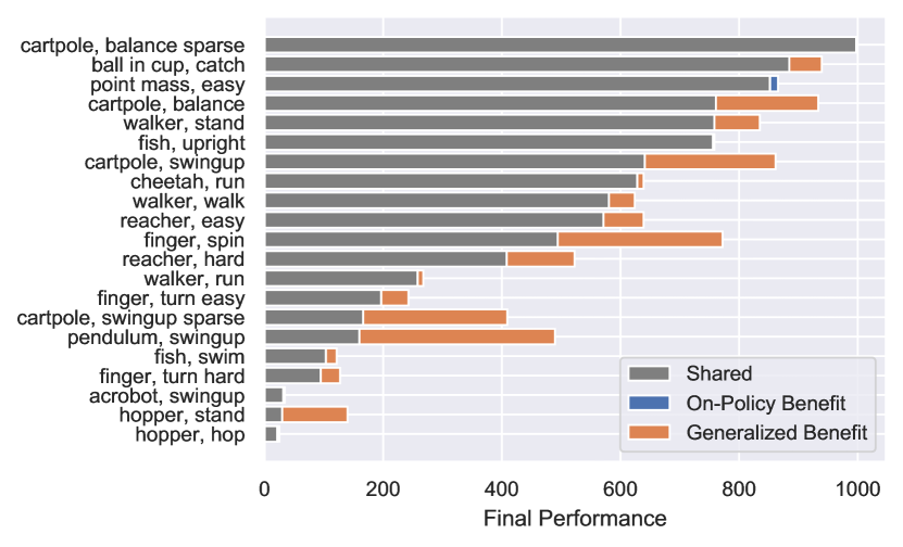
Figure 3: Generalized vs. on-policy final performance by task. Bars represent final performance of the best performing GPI algorithm and the best performing on-policy algorithm. Excludes 7 tasks where no learning occurs under any algorithm. Sorted from high to low based on on-policy performance.

In order to generalize VMPO, we begin by approximating the GPI update in Definition 6 with the reverse KL divergence trust region from (10). In the generalized setting, the new and current state-action visitation distributions $\psi,\psi_{k}$ used in the non-parametric update step are given by

$$\begin{split}\psi(s,a)&=\mathop{\mathbb{E}}_{i\sim\nu}\left[d^{\pi_{k-i}}(s)\right]\pi(a\mid s),\\ \psi_{k}(s,a)&=\mathop{\mathbb{E}}_{i\sim\nu}\left[d^{\pi_{k-i}}(s)\right]\pi_{k}(a\mid s).\end{split}$$

Using these generalized visitation distributions, the non-parametric update has the same form as (17) with $\delta$ replaced by $\delta_{\textnormal{GPI}}$. This results in the target distribution

$$\psi_{\textnormal{targ}}(s,a)=\mathop{\mathbb{E}}_{i\sim\nu}\left[d^{\pi_{k-i}}(s)\right]\pi_{k}(a\mid s)w(s,a),$$

where $w(s,a)$ has the same form as in the on-policy case, the normalizing coefficient is now given by

$$Z(\lambda^{*})=\mathop{\mathbb{E}}_{i\sim\nu}\left[\mathop{\mathbb{E}}_{(s,a)\sim d^{\pi_{k-i}}}\left[\frac{\pi_{k}(a\mid s)}{\pi_{k-i}(a\mid s)}\exp\left(\nicefrac{{A^{\pi_{k}}(s,a)}}{{\lambda^{*}}}\right)\right]\right],$$

and $\lambda^{*}$ is the optimal solution to the corresponding dual problem as in the on-policy case.

The projection step in the generalized case considers the forward KL divergence trust region in (9), resulting in the Generalized VMPO (GeVMPO) update

$$\begin{split}\pi_{k+1}=\arg\max_{\pi}\,\,&\mathop{\mathbb{E}}_{i\sim\nu}\Bigg{[}\mathop{\mathbb{E}}_{(s,a)\sim d^{\pi_{k-i}}}\bigg{[}\\ &\qquad\frac{\pi_{k}(a\mid s)}{\pi_{k-i}(a\mid s)}w(s,a)\log\pi(a\mid s)\bigg{]}\Bigg{]}\\ \textnormal{s.t.}\,\,&\mathop{\mathbb{E}}_{i\sim\nu}\left[\mathop{\mathbb{E}}_{s\sim d^{\pi_{k-i}}}\left[\operatorname{KL}\left(\pi_{k}\|\pi\right)(s)\right]\right]\leq\delta_{\textnormal{GPI}}.\end{split}$$ (19)

7 Experiments

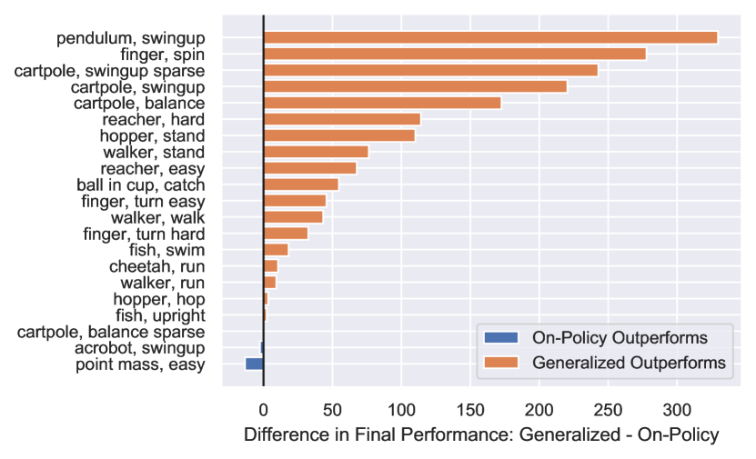
Figure 4: Difference between generalized and on-policy final performance by task. Bars represent difference in final performance between the best performing GPI algorithm and the best performing on-policy algorithm. Excludes 7 tasks where no learning occurs under any algorithm. Sorted from high to low.

In order to analyze the performance of our GPI algorithms, we consider the full set of 28 continuous control benchmark tasks in the DeepMind Control Suite [24]. This benchmark set covers a broad range of continuous control tasks, including a variety of classic control, goal-oriented manipulation, and locomotion tasks. In addition, the benchmark tasks vary in complexity, both in terms of dimensionality and sparsity of reward signals. Finally, each task has a horizon length of $1{,}000$ and $r(s,a)\in[0,1]$ for every state-action pair, resulting in a total return between $0$ and $1{,}000$.

We focus our analysis on the comparison between GPI algorithms and their on-policy policy improvement counterparts. Note that we do not claim state-of-the-art performance, but instead we are interested in evaluating the benefits of theoretically supported sample reuse in the context of policy improvement algorithms. By doing so, we can support the use of GPI algorithms in settings where on-policy methods are currently the most viable option for data-driven control.

In our experiments, we consider default network architectures and hyperparameters commonly found in the literature [26, 27, 28]. We model the policy $\pi$ as a multivariate Gaussian distribution with diagonal covariance, where the mean action for a given state is parameterized by a neural network with two hidden layers of 64 units each and tanh activations. The state-independent standard deviation of each action dimension is parameterized separately. We represent the value function using a neural network with the same structure. For each task, we train our policy for a total of 1 million steps, and we average over 5 random seeds. Note that some of the more difficult, high-dimensional tasks do not demonstrate meaningful learning under these default choices for any of the policy improvement algorithms we consider. These tasks likely require significantly longer training, different network architectures, or other algorithmic frameworks to successfully learn.

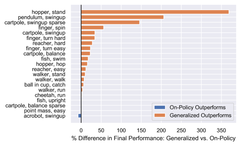
Figure 5: Percent difference between generalized and on-policy final performance by task. Bars represent percent difference in final performance between the best performing GPI algorithm and the best performing on-policy algorithm. Excludes 7 tasks where no learning occurs under any algorithm. Sorted from high to low.

We evaluate performance across three on-policy policy improvement algorithms: PPO, TRPO, and VMPO. For these on-policy algorithms, we consider the default batch size of $N=2{,}048$, which we write as $B=2$ and $n=1{,}024$ since every task we consider has a horizon length of $1{,}000$. We consider $\epsilon=0.2$ for the TV distance trust region parameter in Definition 2, which corresponds to the clipping parameter $\epsilon$ in PPO. We calculate the KL divergence trust region parameter for TRPO and VMPO according to Lemma 3, which results in $\delta=0.02$. We estimate advantages using Generalized Advantage Estimation (GAE) [50].

We also consider generalized versions of each on-policy algorithm: GePPO, GeTRPO, and GeVMPO. When selecting the mixture distribution over prior policies according to Theorem 9, we consider the trade-off parameter with the best final performance from the set of $\kappa=0.0,0.5,1.0$. These choices of trade-off parameter lead to the policy weights in Fig. 2. The generalized trust region parameters $\epsilon_{\textnormal{GPI}}$ and $\delta_{\textnormal{GPI}}$ are calculated according to Theorem 8 and Lemma 7, respectively. As in the on-policy case, our GPI algorithms require estimates of $A^{\pi_{k}}(s,a)$. In order to accomplish this, we consider an off-policy variant of GAE that uses the V-trace value function estimator [51]. See the Appendix for details, including the values of all hyperparameters.

7.1 Overview of Experimental Results

In order to evaluate the benefit of our generalized framework, we compare the best performing on-policy algorithm to the best performing GPI algorithm for every task where learning occurs. Fig. 3 shows the final performance of these algorithms by task, and Fig. 4 shows the difference in final performance by task. From these results, we see a clear performance gain from our generalized approach. Out of 28 tasks, our GPI algorithms outperform in 19 tasks, on-policy algorithms outperform in 2 tasks, and we observe no meaningful learning under any algorithm in 7 tasks when compared to a random policy. In the 2 tasks where on-policy algorithms outperform, the performance difference is small. On the other hand, in the tasks where our GPI algorithms outperform, we often observe a significant performance difference. Fig. 5 shows the percent difference in final performance by task, where we see an improvement of more than 50% from our GPI algorithms in 4 of the tasks and an improvement of more than 10% in 13 of the tasks. Note that we also observe similar trends when comparing any on-policy algorithm to its corresponding generalized version, as summarized in Table 1. See the Appendix for details.

Table 1: Task Classification by Algorithm

Task Classification	PPO	TRPO	VMPO	Best
On-Policy Outperforms	3	1	3	2
Generalized Outperforms	18	19	17	19
No Learning	7	8	8	7
Total Number of Tasks	28	28	28	28

7.2 Analysis of Sparse Reward Tasks

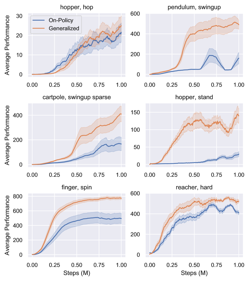
Figure 6: Generalized vs. on-policy performance throughout training for sparse reward tasks. Training curves represent performance of the best performing GPI algorithm and the best performing on-policy algorithm. Shading denotes half of one standard error. Sorted in reading order from most to least sparse.

From Fig. 4 and Fig. 5, it is clear that our generalized framework results in improved performance across a broad range of tasks. This benefit is most pronounced for tasks with sparse reward signals that are difficult to find and exploit. In order to quantify the sparsity of every task in the benchmarking set, we measure the percentage of samples that contain a non-negligible reward signal under a random policy. We measure this statistic by collecting $100{,}000$ samples under a random policy, and calculating the percentage of these samples where $r(s,a)>0.01$.

In 6 of the benchmarking tasks where learning occurs, a random policy receives a reward signal less than 1% of the time. These represent the tasks with the highest level of sparsity, and Fig. 6 shows the performance throughout training for each of them. We note that our generalized approach results in improved performance in all of these sparse reward tasks. In fact, the 3 tasks where our GPI algorithms demonstrate the largest total gain in performance and the 4 tasks where our GPI algorithms demonstrate the largest percentage gain in performance are all contained in this set of sparse reward tasks. In this setting, on-policy algorithms struggle to exploit the limited reward information. The sample reuse in our GPI algorithms, on the other hand, allows sparse reward signals to be exploited across several policy updates while also leading to larger, more diverse batches of data at every update. Together, these benefits of sample reuse result in improved learning progress in difficult sparse reward settings.

8 Conclusion

In this work, we have developed a class of Generalized Policy Improvement algorithms that guarantee approximate policy improvement throughout training while reusing data from all recent policies. We demonstrated the theoretical benefits of principled sample reuse, and showed empirically that our generalized approach results in improved performance compared to popular on-policy algorithms across a variety of continuous control tasks from the DeepMind Control Suite. In particular, our algorithms accelerate learning in difficult sparse reward settings where on-policy algorithms perform poorly.

Because our methods use on-policy policy improvement algorithms as a starting point, our Generalized Policy Improvement lower bound only supports the reuse of data from recent policies. An interesting avenue for future work includes the development of policy improvement guarantees that are compatible with the aggressive sample reuse in off-policy algorithms. Off-policy methods are often very data efficient when properly tuned, and the design of practical performance guarantees for these algorithms may increase their adoption in real-world control settings where large replay buffers are feasible.

9 Detailed Experimental Results

In this section, we provide detailed experimental results that were not included in Section 7. We include full training curves in Fig. 7 for the best performing GPI algorithm and the best performing on-policy algorithm across all tasks where learning occurs. In addition, we include details on final performance across all algorithms and all tasks. Fig. 8 shows a comparison of final performance between generalized and on-policy methods for each choice of policy improvement algorithm. We see similar trends across all algorithms, where our generalized approach results in performance improvement across the majority of tasks in the DeepMind Control Suite benchmarking set. The final performance of every algorithm across each task is included in Table 2, as well as the sparsity metric associated with each task and the performance of a random Gaussian policy with zero mean and unit standard deviation in each action dimension. We say that learning occurs for a task if the best performing algorithm exceeds the performance of the random policy by at least 10.

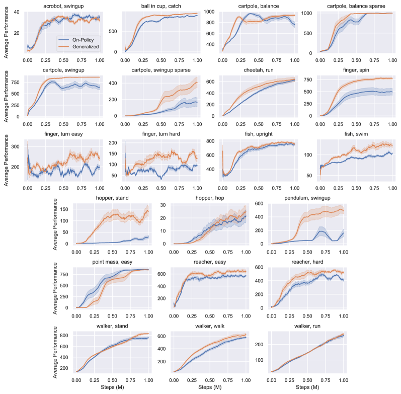
Figure 7: Generalized vs. on-policy performance throughout training by task. Training curves represent performance of the best performing GPI algorithm and the best performing on-policy algorithm. Shading denotes half of one standard error. Excludes 7 tasks where no learning occurs under any algorithm.

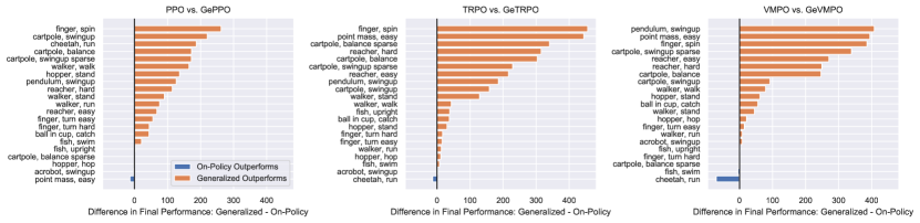
Figure 8: Difference between generalized and on-policy final performance by algorithm and by task. Bars represent difference in final performance between the GPI algorithm and the on-policy algorithm. Excludes 7 tasks where no learning occurs under any algorithm. Sorted from high to low within each algorithm comparison.

Table 2: Final Performance across all Algorithms and Tasks

	Sparsity		PPO		TRPO		VMPO
Task	Metric	Random	On	GPI	On	GPI	On	GPI
acrobot, swingup	2%	3	34	32	21	24	16	24
acrobot, swingup sparse *	0%	0	1	1	1	1	0	1
ball in cup, catch	6%	55	835	879	885	922	884	939
cartpole, balance	92%	322	761	933	320	624	385	631
cartpole, balance sparse	4%	43	998	998	69	410	280	279
cartpole, swingup	56%	47	641	862	574	733	620	712
cartpole, swingup sparse	0%	0	166	339	56	285	70	409
cheetah, run	15%	5	452	639	629	615	594	524
finger, spin	0%	3	494	757	316	772	343	729
finger, turn easy	19%	194	187	243	176	192	197	211
finger, turn hard	9%	88	83	127	82	99	95	96
fish, upright	71%	299	756	758	716	754	732	734
fish, swim	93%	65	100	122	93	101	104	99
hopper, stand	0%	1	3	140	19	50	30	92
hopper, hop	0%	0	22	21	2	13	4	25
humanoid, stand *	1%	5	6	7	6	7	6	6
humanoid, walk *	1%	1	2	2	2	2	2	2
humanoid, run *	1%	1	1	1	1	1	1	1
manipulator, bring ball *	0%	0	1	0	1	0	0	1
pendulum, swingup	0%	0	73	199	160	346	82	490
point mass, easy	1%	4	866	852	141	585	12	406
reacher, easy	5%	50	572	639	379	596	309	580
reacher, hard	1%	8	408	523	104	420	116	365
swimmer, swimmer6 *	68%	192	162	192	154	174	157	178
swimmer, swimmer15 *	69%	178	146	157	145	153	146	154
walker, stand	100%	138	516	607	706	835	759	804
walker, walk	96%	40	426	590	581	624	541	620
walker, run	94%	25	115	191	254	268	258	267
Bold indicates best performing algorithm for each task where learning occurs.
Asterisk (*) indicates no learning occurs under any algorithm.

10 Implementation Details

10.1 Policy Updates

In this section, we provide additional implementation details for GePPO, GeTRPO, and GeVMPO.

10.1.1 GePPO

Because the GePPO objective in (14) is maximized using minibatch stochastic gradient ascent, the effectiveness of the clipping mechanism in enforcing the corresponding trust region depends on the learning rate. To see why this is true, note that each probability ratio begins at the center of the clipping range at the start of each policy update. Therefore, the clipping mechanism has no impact at the beginning of each update, and a large learning rate can result in probability ratios far outside of the clipping range [27].

In order to address this concern, we propose an adaptive learning rate where we decrease the learning rate if the expected TV distance of a policy update exceeds the target trust region radius. See Algorithm 3 for details. This allows the theoretical connection between the clipping mechanism and the TV distance trust region to also hold in practice. Note that this is similar to decaying learning rate schedules which are commonly used in PPO [27, 28], but our approach automatically adapts to satisfy our goal of approximate policy improvement. For the experimental analysis in Section 7, we apply our adaptive learning rate to both PPO and GePPO.

Input: TV distance trust region parameter $\epsilon_{\textnormal{GPI}}$; policy learning rate $\eta$; adaptive learning rate factor $\alpha\geq 0$.

Calculate sample-based estimate $\widehat{\operatorname{TV}}$ of one-step TV distance trust region in Definition 6. if $\widehat{\operatorname{TV}}>\nicefrac{{\epsilon_{\textnormal{GPI}}}}{{2}}$ then  $\eta=\nicefrac{{\eta}}{{(1+\alpha)}}$.

Algorithm 3 GePPO Adaptive Learning Rate

10.1.2 GeTRPO

TRPO considers a first-order expansion of the surrogate objective and second-order expansion of the forward KL divergence trust region in (15), leading to the approximations

$$\mathop{\mathbb{E}}_{(s,a)\sim d^{\pi_{k}}}\left[\frac{\pi(a\mid s)}{\pi_{k}(a\mid s)}A^{\pi_{k}}(s,a)\right]\approx\mathbf{g}_{k}^{\prime}\left(\boldsymbol{\theta}-\boldsymbol{\theta}_{k}\right),$$

$$\mathop{\mathbb{E}}_{s\sim d^{\pi_{k}}}\left[\operatorname{KL}\left(\pi_{k}\|\pi\right)(s)\right]\approx\frac{1}{2}\left(\boldsymbol{\theta}-\boldsymbol{\theta}_{k}\right)^{\prime}\mathbf{F}_{k}\left(\boldsymbol{\theta}-\boldsymbol{\theta}_{k}\right),$$

where $\boldsymbol{\theta},\boldsymbol{\theta}_{k}\in\mathbb{R}^{d}$ are the parameterizations of $\pi$ and $\pi_{k}$, respectively. Using these approximations, the TRPO policy update admits a closed-form solution for the parameterization of $\pi_{k+1}$ given by $\boldsymbol{\theta}_{k+1}=\boldsymbol{\theta}_{k}+\beta\mathbf{v}$, where $\mathbf{v}=\mathbf{F}_{k}^{-1}\mathbf{g}_{k}$ is the update direction and $\beta=\sqrt{\nicefrac{{2\delta}}{{\mathbf{v}^{\prime}\mathbf{F}_{k}\mathbf{v}}}}$. Note that the update direction cannot be calculated directly in high dimensions, so instead it is approximated by applying a finite number of conjugate gradient steps to $\mathbf{F}_{k}\mathbf{v}=\mathbf{g}_{k}$. Finally, a backtracking line search is performed to guarantee that the trust region is satisfied.

The GeTRPO update follows the same procedure, where approximations to the surrogate objective and trust region in (16) are given by

$$\mathop{\mathbb{E}}_{i\sim\nu}\left[\mathop{\mathbb{E}}_{(s,a)\sim d^{\pi_{k-i}}}\left[\frac{\pi(a\mid s)}{\pi_{k-i}(a\mid s)}A^{\pi_{k}}(s,a)\right]\right]\approx\mathbf{g}_{k,\nu}^{\prime}\left(\boldsymbol{\theta}-\boldsymbol{\theta}_{k}\right),$$

$$\mathop{\mathbb{E}}_{i\sim\nu}\left[\mathop{\mathbb{E}}_{s\sim d^{\pi_{k-i}}}\left[\operatorname{KL}\left(\pi_{k}\|\pi\right)(s)\right]\right]\approx\frac{1}{2}\left(\boldsymbol{\theta}-\boldsymbol{\theta}_{k}\right)^{\prime}\mathbf{F}_{k,\nu}\left(\boldsymbol{\theta}-\boldsymbol{\theta}_{k}\right),$$

which represent first-order and second-order expansions, respectively, centered around $\pi_{k}$.

10.1.3 GeVMPO

In order to implement the VMPO update in (18), we approximate expectations using sample averages. Because we only have access to a single action in any given state, the empirical version of the maximum likelihood objective in (18) incentivizes an increase in likelihood at every state-action pair, even those with $w(s,a)<1$. In order to address this issue, [23] only considered samples with positive advantages. Rather than discard potentially useful information from half of the collected samples, we propose an alternative approach. We note the similarity between the VMPO update in (18) and the TRPO update in (15), where the only difference comes in the form of the objective. Therefore, we can apply the same optimization procedure as in TRPO, where we consider a first-order approximation of the objective and a second-order approximation of the forward KL divergence trust region. Similar to policy gradient methods, we introduce a baseline value to the objective that does not impact the gradient at the current policy $\pi_{k}$ [52]. In particular, we replace the non-parametric target weights $w(s,a)$ in (18) with $\bar{w}(s,a)=w(s,a)-1$. This leads to the same gradient as the true maximum likelihood objective at $\pi_{k}$, but results in the appropriate update direction at every state-action pair when we approximate expectations using sample averages. This addresses the issue with the empirical maximum likelihood objective noted above, while still allowing us to make use of every sample we have collected.

As in the VMPO update, we also replace the weights $w(s,a)$ with $\bar{w}(s,a)$ for the GeVMPO update in (19). Then, we apply the same optimization procedure as in GeTRPO to calculate the GeVMPO update.

10.2 Advantage Estimation

In all of the policy improvement algorithms we consider, we must estimate the advantage function $A^{\pi_{k}}(s,a)$ of the current policy $\pi_{k}$. The use of $A^{\pi_{k}}(s,a)$ is important because it allows our methods to provide policy improvement guarantees with respect to the current policy, regardless of the policy used to generate the data. In the on-policy setting, advantage estimation is straightforward because multi-step advantage estimates are unbiased except for the use of bootstrapping with the learned value function. We use Generalized Advantage Estimation (GAE) [50] with $\lambda=0.97$ in all on-policy algorithms, where $\lambda$ determines a weighted average over $K$-step advantage estimates.

When estimating $A^{\pi_{k}}(s,a)$ in our GPI algorithms, on the other hand, our data has been collected using prior policies. As a result, the multi-step estimates used in GAE are no longer unbiased. Therefore, we must use off-policy estimation techniques to account for this bias. We consider an off-policy variant of GAE that uses the V-trace value function estimator [51], which corrects multi-step off-policy estimates while controlling variance via truncated importance sampling. For data collected under a prior policy $\pi_{k-i}$, the $K$-step V-trace estimate of the current value function is given by

$$V^{\pi_{k}}_{\textnormal{trace}}(s_{t})=V(s_{t})+\sum_{j=0}^{K-1}\gamma^{j}\left(\prod_{m=0}^{j}c_{t+m}\right)\delta_{t+j}^{V},$$

where $V$ is a learned value function, $\delta_{t}^{V}=r(s_{t},a_{t})+\gamma V(s_{t+1})-V(s_{t})$, and $c_{t}=\min(\,\bar{c},\,\nicefrac{{\pi_{k}(a_{t}\mid s_{t})}}{{\pi_{k-i}(a_{t}\mid s_{t})}}\,)$ represents a truncated importance sampling ratio with truncation parameter $\bar{c}$. Similarly, for $K\geq 2$, the corrected $K$-step estimate of the current advantage function using V-trace is given by

$$A^{\pi_{k}}_{\textnormal{trace}}(s_{t},a_{t})=\delta_{t}^{V}+\sum_{j=1}^{K-1}\gamma^{j}\left(\prod_{m=1}^{j}c_{t+m}\right)\delta_{t+j}^{V},$$

and for $K=1$ we have the standard one-step estimate $A^{\pi_{k}}_{\textnormal{trace}}(s_{t},a_{t})=\delta_{t}^{V}$ that does not require any correction. Note that [51] treat the final importance sampling ratio in each term separately, but we do not make this distinction in our notation because the truncation parameter is typically chosen to be the same for all terms. We use the default setting of $\bar{c}=1$ from [51] in our experiments, and as in GAE we consider a weighted average over $K$-step estimates determined by the parameter $\lambda$.

It is common to standardize advantage estimates within each batch or minibatch during policy updates. Note that the expectation of $A^{\pi_{k}}(s,a)$ with respect to samples generated under the current policy $\pi_{k}$ equals zero, so standardization ensures that our sample-based estimates also satisfy this property. Therefore, the appropriate quantity to standardize in the generalized case is

$$\frac{\pi_{k}(a\mid s)}{\pi_{k-i}(a\mid s)}A^{\pi_{k}}(s,a),$$

since the expectation of this term with respect to data generated under prior policies equals zero.

10.3 Hyperparameter Values

We provide the values of all hyperparameters used for our experimental analysis in Table 3. In addition, we describe how to calculate the scaling coefficients $c_{\textnormal{ESS}},c_{\textnormal{TV}}$ used when determining the optimal mixture distribution in Theorem 9. We include these coefficients in Theorem 9 so that each component of the objective is on the same scale, which we can accomplish by setting each coefficient to be the range of potential values for its corresponding numerator. The numerator in the effective sample size term is the largest when $\kappa=0$ and smallest when $\kappa=1$, and the reverse is true for the numerator in the total TV distance update size term. Therefore, we set the scaling coefficients to be

$$c_{\textnormal{ESS}} =\sum_{i}\nu_{i}^{*}(0)^{2}-\sum_{i}\nu_{i}^{*}(1)^{2},$$

$$c_{\textnormal{TV}} =\sum_{i}\nu_{i}^{*}(1)(i+1)-\sum_{i}\nu_{i}^{*}(0)(i+1),$$

where $\nu^{*}(0)$ and $\nu^{*}(1)$ are the optimal mixture distributions when $\kappa=0$ and $\kappa=1$, respectively. Note that we can calculate these optimal mixture distributions by ignoring the scaling coefficients in Theorem 9, since the coefficients do not impact the resulting minimizer for these extreme values of trade-off parameter $\kappa$.

Table 3: Hyperparameter Values for Experimental Results

General
Discount rate ($\gamma$)	$0.995$
GAE parameter ($\lambda$)	$0.97$
Value function optimizer	Adam
Value function learning rate	$3\mathrm{e}{-4}$
Value function minibatches per epoch	$32$
Value function epochs per update	$10$
V-trace truncation parameter ($\bar{c}$)	$1.0$
On-policy batch size ($N$)	$2{,}048$
Minimum batch size ($n$)	$1{,}024$
Trade-off parameter ($\kappa$)	$0.0,0.5,1.0$
Initial policy standard deviation	$1.0$
Trust region parameter ($\epsilon$)	$0.2$
PPO
Policy optimizer	Adam
Initial policy learning rate ($\eta$)	$3\mathrm{e}{-4}$
Adaptive learning rate factor ($\alpha$)	$0.03$
Policy minibatches per epoch	$32$
Policy epochs per update	$10$
TRPO / VMPO
Conjugate gradient iterations per update	$20$
Conjugate gradient damping coefficient	$0.01$

11 Proofs

11.1 Proof of Lemma 3

Proof 11.12.

Note that TV distance is symmetric, so the same argument can be used starting from (3) or (4). By applying Pinsker’s inequality followed by Jensen’s inequality, we see that

$$\begin{split}\mathop{\mathbb{E}}_{s\sim d^{\pi_{k}}}\left[\operatorname{TV}\left(\pi,\pi_{k}\right)(s)\right]\,&\leq\,\sqrt{\frac{1}{2}\mathop{\mathbb{E}}_{s\sim d^{\pi_{k}}}\left[\operatorname{KL}\left(\pi\|\pi_{k}\right)(s)\right]}\\ &\leq\,\sqrt{\frac{\delta}{2}}\,=\,\frac{\epsilon}{2}.\end{split}$$

11.2 Proof of Lemma 4

We will make use of the following results in our proof.

Lemma 11.13 (From [25]).

Consider any policy $\pi$ and a current policy $\pi_{k}$. Then,

$$J(\pi)-J(\pi_{k})=\frac{1}{1-\gamma}\mathop{\mathbb{E}}_{s\sim d^{\pi}}\left[\mathop{\mathbb{E}}_{a\sim\pi(\,\cdot\,\mid s)}\left[A^{\pi_{k}}(s,a)\right]\right].$$

Lemma 11.14 (From [10]).

Consider any policy $\pi$ and a reference policy $\pi_{\textnormal{ref}}$. Then,

$$\operatorname{TV}\left(d^{\pi},d^{\pi_{\textnormal{ref}}}\right)\leq\frac{\gamma}{1-\gamma}\mathop{\mathbb{E}}_{s\sim d^{\pi_{\textnormal{ref}}}}\left[\operatorname{TV}\left(\pi,\pi_{\textnormal{ref}}\right)(s)\right],$$

where $d^{\pi}$ and $d^{\pi_{\textnormal{ref}}}$ represent normalized discounted state visitation distributions.

We are now ready to prove Lemma 4.

Proof 11.15.

We apply similar proof techniques as in [10], but we are interested in $d^{\pi_{\textnormal{ref}}}$ as our sampling distribution rather than $d^{\pi_{k}}$. Starting from the equality in Lemma 11.13, we add and subtract the term

$$\frac{1}{1-\gamma}\mathop{\mathbb{E}}_{s\sim d^{\pi_{\textnormal{ref}}}}\left[\mathop{\mathbb{E}}_{a\sim\pi(\,\cdot\,\mid s)}\left[A^{\pi_{k}}(s,a)\right]\right].$$

By doing so, we have

$$J(\pi)-J(\pi_{k})$$

$$\quad=\frac{1}{1-\gamma}\mathop{\mathbb{E}}_{s\sim d^{\pi_{\textnormal{ref}}}}\left[\mathop{\mathbb{E}}_{a\sim\pi(\,\cdot\,\mid s)}\left[A^{\pi_{k}}(s,a)\right]\right]$$

$$\qquad\qquad+\frac{1}{1-\gamma}\bigg{(}\mathop{\mathbb{E}}_{s\sim d^{\pi}}\left[\mathop{\mathbb{E}}_{a\sim\pi(\,\cdot\,\mid s)}\left[A^{\pi_{k}}(s,a)\right]\right]$$

$$\qquad\qquad\qquad\qquad-\mathop{\mathbb{E}}_{s\sim d^{\pi_{\textnormal{ref}}}}\left[\mathop{\mathbb{E}}_{a\sim\pi(\,\cdot\,\mid s)}\left[A^{\pi_{k}}(s,a)\right]\right]\bigg{)}$$

$$\quad\geq\frac{1}{1-\gamma}\mathop{\mathbb{E}}_{s\sim d^{\pi_{\textnormal{ref}}}}\left[\mathop{\mathbb{E}}_{a\sim\pi(\,\cdot\,\mid s)}\left[A^{\pi_{k}}(s,a)\right]\right]$$

$$\qquad\qquad-\frac{1}{1-\gamma}\bigg{|}\mathop{\mathbb{E}}_{s\sim d^{\pi}}\left[\mathop{\mathbb{E}}_{a\sim\pi(\,\cdot\,\mid s)}\left[A^{\pi_{k}}(s,a)\right]\right]$$

$$\qquad\qquad\qquad\qquad-\mathop{\mathbb{E}}_{s\sim d^{\pi_{\textnormal{ref}}}}\left[\mathop{\mathbb{E}}_{a\sim\pi(\,\cdot\,\mid s)}\left[A^{\pi_{k}}(s,a)\right]\right]\bigg{|}.$$ (20)

Next, we can bound the magnitude of the second term in the right-hand side of (20). Ignoring the constant multiplicative factor, we have that

$$\bigg{|}\mathop{\mathbb{E}}_{s\sim d^{\pi}}\left[\mathop{\mathbb{E}}_{a\sim\pi(\,\cdot\,\mid s)}\left[A^{\pi_{k}}(s,a)\right]\right]-\mathop{\mathbb{E}}_{s\sim d^{\pi_{\textnormal{ref}}}}\left[\mathop{\mathbb{E}}_{a\sim\pi(\,\cdot\,\mid s)}\left[A^{\pi_{k}}(s,a)\right]\right]\bigg{|}$$

$$\,\,\leq\max_{s\in\mathcal{S}}\left|\mathop{\mathbb{E}}_{a\sim\pi(\,\cdot\,\mid s)}\left[A^{\pi_{k}}(s,a)\right]\right|\cdot\int_{\mathcal{S}}\left|d^{\pi}(s)-d^{\pi_{\textnormal{ref}}}(s)\right|\textnormal{d}s$$ (21)

$$\,\,=2C^{\pi,\pi_{k}}\cdot\operatorname{TV}\left(d^{\pi},d^{\pi_{\textnormal{ref}}}\right)$$ (22)

$$\,\,\leq\frac{2\gamma C^{\pi,\pi_{k}}}{1-\gamma}\mathop{\mathbb{E}}_{s\sim d^{\pi_{\textnormal{ref}}}}\left[\operatorname{TV}\left(\pi,\pi_{\textnormal{ref}}\right)(s)\right],$$ (23)

where we have used Hölder’s inequality in (21), the definition of $C^{\pi,\pi_{k}}$ from Lemma 1 and the definition of TV distance in (22), and Lemma 11.14 in (23). This results in the lower bound

$$J(\pi)-J(\pi_{k})\geq\frac{1}{1-\gamma}\mathop{\mathbb{E}}_{s\sim d^{\pi_{\textnormal{ref}}}}\left[\mathop{\mathbb{E}}_{a\sim\pi(\,\cdot\,\mid s)}\left[A^{\pi_{k}}(s,a)\right]\right]\\ -\frac{2\gamma C^{\pi,\pi_{k}}}{(1-\gamma)^{2}}\mathop{\mathbb{E}}_{s\sim d^{\pi_{\textnormal{ref}}}}\left[\operatorname{TV}\left(\pi,\pi_{\textnormal{ref}}\right)(s)\right].$$

Finally, we apply importance sampling on the actions in the first term to obtain the result, which assumes that the support of $\pi$ is contained within the support of $\pi_{\textnormal{ref}}$ at every state.

11.3 Proof of Theorem 5

Proof 11.16.

For any prior policy $\pi_{k-i}$, we can apply Lemma 4 to construct a policy improvement lower bound with expectations that depend on the visitation distribution $d^{\pi_{k-i}}$. These all represent lower bounds on the same quantity $J(\pi)-J(\pi_{k})$, so any convex combination of these lower bounds will also be a lower bound on $J(\pi)-J(\pi_{k})$. Therefore, (5) holds for any choice of mixture distribution $\nu$ over prior policies.

11.4 Proof of Lemma 7

Proof 11.17.

As in the proof of Lemma 3, we apply Pinsker’s inequality followed by Jensen’s inequality to the left-hand side of the trust region constraint in (8). By doing so, we have that

$$\mathop{\mathbb{E}}_{i\sim\nu}\left[\mathop{\mathbb{E}}_{s\sim d^{\pi_{k-i}}}\left[\operatorname{TV}\left(\pi,\pi_{k}\right)(s)\right]\right]\\ \leq\sqrt{\frac{1}{2}\mathop{\mathbb{E}}_{i\sim\nu}\left[\mathop{\mathbb{E}}_{s\sim d^{\pi_{k-i}}}\left[\operatorname{KL}\left(\pi\|\pi_{k}\right)(s)\right]\right]}\leq\sqrt{\frac{\delta_{\textnormal{GPI}}}{2}}=\frac{\epsilon_{\textnormal{GPI}}}{2}.$$

11.5 Proof of Theorem 8

Proof 11.18.

The coefficients outside of the expectation in the on-policy and generalized penalty terms are the same, so we need to show that the trust region in (6) is satisfied to prove the claim. For ease of notation, we write $\pi=\pi_{k+1}$. Using the triangle inequality for TV distance, we have that

$$\begin{split}&\mathop{\mathbb{E}}_{i\sim\nu}\left[\mathop{\mathbb{E}}_{s\sim d^{\pi_{k-i}}}\left[\operatorname{TV}\left(\pi,\pi_{k-i}\right)(s)\right]\right]\\ &\qquad\leq\mathop{\mathbb{E}}_{i\sim\nu}\left[\sum_{j=0}^{i}\mathop{\mathbb{E}}_{s\sim d^{\pi_{k-i}}}\left[\operatorname{TV}\left(\pi_{k-j+1},\pi_{k-j}\right)(s)\right]\right]\\ &\qquad\leq\mathop{\mathbb{E}}_{i\sim\nu}\left[\frac{\epsilon_{\textnormal{GPI}}}{2}\cdot\left(i+1\right)\right]=\frac{\epsilon_{\textnormal{GPI}}}{2}\cdot\mathop{\mathbb{E}}_{i\sim\nu}\left[\,i+1\,\right]=\frac{\epsilon}{2},\end{split}$$

where we have used the assumption on the expected one-step TV distance under each state visitation distribution to bound each term inside the summation by $\nicefrac{{\epsilon_{\textnormal{GPI}}}}{{2}}$.

11.6 Proof of Theorem 9

Proof 11.19.

Note that $f_{\textnormal{ESS}}(\nu)$ and $f_{\textnormal{TV}}(\nu)$ only depend on $\nu$ in their denominators. Therefore, we can maximize these quantities by minimizing the quantities in their denominators that depend on $\nu$. By considering a convex combination determined by the trade-off parameter $\kappa$ and applying scaling coefficients, we arrive at the objective in (12).

Next, we consider the constraints in (12). The first constraint implies $f_{\textnormal{ESS}}(\nu)\geq Bn$ and the second constraint implies $f_{\textnormal{TV}}(\nu)\geq\nicefrac{{\epsilon}}{{2}}$. Therefore, these constraints guarantee that the effective sample size and total TV distance update size are at least as large as in the on-policy case. The remaining constraints ensure that $\nu$ is a distribution.

Finally, note that a uniform distribution over the last $M$ policies is a feasible solution to (12) for $B\leq M\leq 2B-1$. Therefore, (12) is a feasible optimization problem.

11.7 Proof of Lemma 10

Proof 11.20.

From the definition of TV distance, we have that

$$\mathop{\mathbb{E}}_{s\sim d^{\pi_{k}}}\left[\operatorname{TV}\left(\pi,\pi_{k}\right)(s)\right]\\ =\frac{1}{2}\mathop{\mathbb{E}}_{s\sim d^{\pi_{k}}}\left[\int_{\mathcal{A}}\left|\pi(a\mid s)-\pi_{k}(a\mid s)\right|\textnormal{d}a\right].$$

Then, by multiplying and dividing each term by $\pi_{k}(a\mid s)$, we obtain the result.

11.8 Proof of Lemma 11

Proof 11.21.

Apply the same techniques as in the proof of Lemma 10. From the definition of TV distance, we have that

$$\mathop{\mathbb{E}}_{i\sim\nu}\left[\mathop{\mathbb{E}}_{s\sim d^{\pi_{k-i}}}\left[\operatorname{TV}\left(\pi,\pi_{k}\right)(s)\right]\right]\\ =\frac{1}{2}\mathop{\mathbb{E}}_{i\sim\nu}\left[\mathop{\mathbb{E}}_{s\sim d^{\pi_{k-i}}}\left[\int_{\mathcal{A}}\left|\pi(a\mid s)-\pi_{k}(a\mid s)\right|\textnormal{d}a\right]\right].$$

Then, by multiplying and dividing each term by $\pi_{k-i}(a\mid s)$, we obtain the result.

References

- [1] L. Buşoniu, T. de Bruin, D. Tolić, J. Kober, and I. Palunko, “Reinforcement learning for control: Performance, stability, and deep approximators,” Annu. Rev. Control, vol. 46, pp. 8–28, 2018.
- [2] B. Recht, “A tour of reinforcement learning: The view from continuous control,” Annu. Rev. Control, Robot., Auton. Syst., vol. 2, no. 1, pp. 253–279, 2019.
- [3] Y. Duan, X. Chen, R. Houthooft, J. Schulman, and P. Abbeel, “Benchmarking deep reinforcement learning for continuous control,” in Proc. 33rd Int. Conf. Mach. Learn., vol. 48, 2016, pp. 1329–1338.
- [4] T. Kurutach, I. Clavera, Y. Duan, A. Tamar, and P. Abbeel, “Model-ensemble trust-region policy optimization,” in Proc. 6th Int. Conf. Learn. Representations, 2018.
- [5] M. Janner, J. Fu, M. Zhang, and S. Levine, “When to trust your model: Model-based policy optimization,” in Proc. Adv. Neural Inf. Process. Syst., vol. 32, 2019.
- [6] A. Rajeswaran, I. Mordatch, and V. Kumar, “A game theoretic framework for model based reinforcement learning,” in Proc. 37th Int. Conf. Mach. Learn., vol. 119, 2020, pp. 7953–7963.
- [7] Y. Wu, G. Tucker, and O. Nachum, “Behavior regularized offline reinforcement learning,” arXiv:1911.11361, 2019.
- [8] A. Kumar, A. Zhou, G. Tucker, and S. Levine, “Conservative Q-learning for offline reinforcement learning,” in Proc. Adv. Neural Inf. Process. Syst., vol. 33, 2020.
- [9] R. Kidambi, A. Rajeswaran, P. Netrapalli, and T. Joachims, “MOReL: Model-based offline reinforcement learning,” in Proc. Adv. Neural Inf. Process. Syst., vol. 33, 2020.
- [10] J. Achiam, D. Held, A. Tamar, and P. Abbeel, “Constrained policy optimization,” in Proc. 34th Int. Conf. Mach. Learn., vol. 70, 2017, pp. 22–31.
- [11] J. F. Fisac, A. K. Akametalu, M. N. Zeilinger, S. Kaynama, J. Gillula, and C. J. Tomlin, “A general safety framework for learning-based control in uncertain robotic systems,” IEEE Trans. Autom. Control, vol. 64, no. 7, pp. 2737–2752, 2019.
- [12] K. P. Wabersich, L. Hewing, A. Carron, and M. N. Zeilinger, “Probabilistic model predictive safety certification for learning-based control,” IEEE Trans. Autom. Control, vol. 67, no. 1, pp. 176–188, 2022.
- [13] L. Brunke, M. Greeff, A. W. Hall, Z. Yuan, S. Zhou, J. Panerati, and A. P. Schoellig, “Safe learning in robotics: From learning-based control to safe reinforcement learning,” Annu. Rev. Control, Robot., Auton. Syst., vol. 5, no. 1, pp. 411–444, 2022.
- [14] S. Paternain, M. Calvo-Fullana, L. F. O. Chamon, and A. Ribeiro, “Safe policies for reinforcement learning via primal-dual methods,” IEEE Trans. Autom. Control, vol. 68, no. 3, pp. 1321–1336, 2023.
- [15] I. Jang, H. Kim, D. Lee, Y.-S. Son, and S. Kim, “Knowledge transfer for on-device deep reinforcement learning in resource constrained edge computing systems,” IEEE Access, vol. 8, pp. 146 588–146 597, 2020.
- [16] B. P. Duisterhof, S. Krishnan, J. J. Cruz, C. R. Banbury, W. Fu, A. Faust, G. C. H. E. de Croon, and V. Janapa Reddi, “Tiny robot learning (tinyRL) for source seeking on a nano quadcopter,” in Proc. IEEE Int. Conf. Robot. Autom., 2021, pp. 7242–7248.
- [17] L. Grossman and B. Plancher, “Just round: Quantized observation spaces enable memory efficient learning of dynamic locomotion,” arXiv:2210.08065, 2022.
- [18] S. M. Neuman, B. Plancher, B. P. Duisterhof, S. Krishnan, C. Banbury, M. Mazumder, S. Prakash, J. Jabbour, A. Faust, G. C. de Croon, and V. J. Reddi, “Tiny robot learning: Challenges and directions for machine learning in resource-constrained robots,” in Proc. IEEE 4th Int. Conf. Artif. Intell. Circuits Syst., 2022, pp. 296–299.
- [19] D. Pau, S. Colella, and C. Marchisio, “End to end optimized tiny learning for repositionable walls in maze topologies,” in Proc. IEEE Int. Conf. Consum. Electron., 2023, pp. 1–7.
- [20] J. Queeney, I. C. Paschalidis, and C. G. Cassandras, “Generalized proximal policy optimization with sample reuse,” in Proc. Adv. Neural Inf. Process. Syst., vol. 34, 2021.
- [21] J. Schulman, F. Wolski, P. Dhariwal, A. Radford, and O. Klimov, “Proximal policy optimization algorithms,” arXiv:1707.06347, 2017.
- [22] J. Schulman, S. Levine, P. Abbeel, M. Jordan, and P. Moritz, “Trust region policy optimization,” in Proc. 32nd Int. Conf. Mach. Learn., vol. 37, 2015, pp. 1889–1897.
- [23] H. F. Song, A. Abdolmaleki, J. T. Springenberg, A. Clark, H. Soyer, J. W. Rae, S. Noury, A. Ahuja, S. Liu, D. Tirumala, N. Heess, D. Belov, M. Riedmiller, and M. M. Botvinick, “V-MPO: On-policy maximum a posteriori policy optimization for discrete and continuous control,” in Proc. 8th Int. Conf. Learn. Representations, 2020.
- [24] S. Tunyasuvunakool, A. Muldal, Y. Doron, S. Liu, S. Bohez, J. Merel, T. Erez, T. Lillicrap, N. Heess, and Y. Tassa, “dm_control: Software and tasks for continuous control,” Softw. Impacts, vol. 6, p. 100022, 2020.
- [25] S. Kakade and J. Langford, “Approximately optimal approximate reinforcement learning,” in Proc. 19th Int. Conf. Mach. Learn., 2002, pp. 267–274.
- [26] P. Henderson, R. Islam, P. Bachman, J. Pineau, D. Precup, and D. Meger, “Deep reinforcement learning that matters,” in Proc. AAAI Conf. Artif. Intell., vol. 32, no. 1, 2018, pp. 3207–3214.
- [27] L. Engstrom, A. Ilyas, S. Santurkar, D. Tsipras, F. Janoos, L. Rudolph, and A. Madry, “Implementation matters in deep RL: A case study on PPO and TRPO,” in Proc. 8th Int. Conf. Learn. Representations, 2020.
- [28] M. Andrychowicz, A. Raichuk, P. Stańczyk, M. Orsini, S. Girgin, R. Marinier, L. Hussenot, M. Geist, O. Pietquin, M. Michalski, S. Gelly, and O. Bachem, “What matters for on-policy deep actor-critic methods? A large-scale study,” in Proc. 9th Int. Conf. Learn. Representations, 2021.
- [29] J. Queeney, I. C. Paschalidis, and C. G. Cassandras, “Uncertainty-aware policy optimization: A robust, adaptive trust region approach,” in Proc. AAAI Conf. Artif. Intell., vol. 35, no. 11, 2021, pp. 9377–9385.
- [30] Y. Wang, H. He, X. Tan, and Y. Gan, “Trust region-guided proximal policy optimization,” in Proc. Adv. Neural Inf. Process. Syst., vol. 32, 2019.
- [31] Y. Wang, H. He, and X. Tan, “Truly proximal policy optimization,” in Proc. 35th Uncertainty Artif. Intell. Conf., vol. 115, 2020, pp. 113–122.
- [32] Y. Cheng, L. Huang, and X. Wang, “Authentic boundary proximal policy optimization,” IEEE Trans. Cybern., vol. 52, no. 9, pp. 9428–9438, 2022.
- [33] Q. Vuong, Y. Zhang, and K. Ross, “Supervised policy update for deep reinforcement learning,” in Proc. 7th Int. Conf. Learn. Representations, 2019.
- [34] A. Abdolmaleki, J. T. Springenberg, Y. Tassa, R. Munos, N. Heess, and M. Riedmiller, “Maximum a posteriori policy optimisation,” in Proc. 6th Int. Conf. Learn. Representations, 2018.
- [35] T. P. Lillicrap, J. J. Hunt, A. Pritzel, N. Heess, T. Erez, Y. Tassa, D. Silver, and D. Wierstra, “Continuous control with deep reinforcement learning,” in Proc. 4th Int. Conf. Learn. Representations, 2016.
- [36] S. Fujimoto, H. van Hoof, and D. Meger, “Addressing function approximation error in actor-critic methods,” in Proc. 35th Int. Conf. Mach. Learn., vol. 80, 2018, pp. 1587–1596.
- [37] T. Haarnoja, A. Zhou, P. Abbeel, and S. Levine, “Soft actor-critic: Off-policy maximum entropy deep reinforcement learning with a stochastic actor,” in Proc. 35th Int. Conf. Mach. Learn., vol. 80, 2018, pp. 1861–1870.
- [38] B. O’Donoghue, R. Munos, K. Kavukcuoglu, and V. Mnih, “Combining policy gradient and Q-learning,” in Proc. 5th Int. Conf. Learn. Representations, 2017.
- [39] S. Gu, T. Lillicrap, Z. Ghahramani, R. E. Turner, and S. Levine, “Q-Prop: Sample-efficient policy gradient with an off-policy critic,” in Proc. 5th Int. Conf. Learn. Representations, 2017.
- [40] S. Gu, T. Lillicrap, R. E. Turner, Z. Ghahramani, B. Schölkopf, and S. Levine, “Interpolated policy gradient: Merging on-policy and off-policy gradient estimation for deep reinforcement learning,” in Proc. Adv. Neural Inf. Process. Syst., vol. 30, 2017.
- [41] W. Meng, Q. Zheng, Y. Shi, and G. Pan, “An off-policy trust region policy optimization method with monotonic improvement guarantee for deep reinforcement learning,” IEEE Trans. Neural Netw. Learn. Syst., vol. 33, no. 5, pp. 2223–2235, 2022.
- [42] R. Fakoor, P. Chaudhari, and A. J. Smola, “P3O: Policy-on policy-off policy optimization,” in Proc. 35th Uncertainty Artif. Intell. Conf., vol. 115, 2020, pp. 1017–1027.
- [43] Z. Wang, V. Bapst, N. Heess, V. Mnih, R. Munos, K. Kavukcuoglu, and N. de Freitas, “Sample efficient actor-critic with experience replay,” in Proc. 5th Int. Conf. Learn. Representations, 2017.
- [44] G. Novati and P. Koumoutsakos, “Remember and forget for experience replay,” in Proc. 36th Int. Conf. Mach. Learn., vol. 97, 2019, pp. 4851–4860.
- [45] C. Wang, Y. Wu, Q. Vuong, and K. Ross, “Striving for simplicity and performance in off-policy DRL: Output normalization and non-uniform sampling,” in Proc. 37th Int. Conf. Mach. Learn., vol. 119, 2020, pp. 10 070–10 080.
- [46] T. Schaul, J. Quan, I. Antonoglou, and D. Silver, “Prioritized experience replay,” in Proc. 4th Int. Conf. Learn. Representations, 2016.
- [47] T. de Bruin, J. Kober, K. Tuyls, and R. Babuška, “Experience selection in deep reinforcement learning for control,” J. Mach. Learn. Res., vol. 19, no. 9, pp. 1–56, 2018.
- [48] Z.-W. Hong, T.-Y. Shann, S.-Y. Su, Y.-H. Chang, T.-J. Fu, and C.-Y. Lee, “Diversity-driven exploration strategy for deep reinforcement learning,” in Proc. Adv. Neural Inf. Process. Syst., vol. 31, 2018.
- [49] A. Kong, “A note on importance sampling using standardized weights,” Tech. Rep. 348, Dept. Statist., Univ. Chicago, 1992.
- [50] J. Schulman, P. Moritz, S. Levine, M. I. Jordan, and P. Abbeel, “High-dimensional continuous control using generalized advantage estimation,” in Proc. 4th Int. Conf. Learn. Representations, 2016.
- [51] L. Espeholt, H. Soyer, R. Munos, K. Simonyan, V. Mnih, T. Ward, Y. Doron, V. Firoiu, T. Harley, I. Dunning, S. Legg, and K. Kavukcuoglu, “IMPALA: Scalable distributed deep-RL with importance weighted actor-learner architectures,” in Proc. 35th Int. Conf. Mach. Learn., vol. 80, 2018, pp. 1407–1416.
- [52] R. S. Sutton, D. McAllester, S. Singh, and Y. Mansour, “Policy gradient methods for reinforcement learning with function approximation,” in Proc. Adv. Neural Inf. Process. Syst., vol. 12, 2000.