Photometric redshift estimates using Bayesian neural networks in the CSST survey

Abstract

Galaxy photometric redshift (photo-$z$) is crucial in cosmological studies, such as weak gravitational lensing and galaxy angular clustering measurements. In this work, we try to extract photo-$z$ information and construct its probability distribution function (PDF) using the Bayesian neural networks (BNN) from both galaxy flux and image data expected to be obtained by the China Space Station Telescope (CSST). The mock galaxy images are generated from the Advanced Camera for Surveys of Hubble Space Telescope ($HST$-ACS) and COSMOS catalog, in which the CSST instrumental effects are carefully considered. And the galaxy flux data are measured from galaxy images using aperture photometry. We construct Bayesian multilayer perceptron (B-MLP) and Bayesian convolutional neural network (B-CNN) to predict photo-$z$ along with the PDFs from fluxes and images, respectively. We combine the B-MLP and B-CNN together, and construct a hybrid network and employ the transfer learning techniques to investigate the improvement of including both flux and image data. For galaxy samples with SNR$>$10 in $g$ or $i$ band, we find the accuracy and outlier fraction of photo-$z$ can achieve $\sigma_{\rm NMAD}=0.022$ and $\eta=2.35\%$ for the B-MLP using flux data only, and $\sigma_{\rm NMAD}=0.022$ and $\eta=1.32\%$ for the B-CNN using image data only. The Bayesian hybrid network can achieve $\sigma_{\rm NMAD}=0.021$ and $\eta=1.23\%$, and utilizing transfer learning technique can improve results to $\sigma_{\rm NMAD}=0.019$ and $\eta=1.17\%$, which can provide the most confident predictions with the lowest average uncertainty.

1 Introduction

According to current cosmological observations, about 95% components of our Universe are dark matter and dark energy, far more abundant than luminous objects. Dark matter and dark energy are major concerns in current cosmological studies, and they leave their footprints at both small and large scales, such as galaxies and large-scale structure. A number of ongoing and next-generation surveys attempt to detect these footprints in wide and deep survey areas, e.g. the Sloan Digital Sky Survey (Fukugita et al. 1996; York et al. 2000), Dark Energy Survey (Collaboration: et al. 2016; Abbott et al. 2021), the Legacy Survey of Space and Time (LSST) or Vera C. Rubin Observatory (LSST Science Collaboration et al. 2009; Ivezić et al. 2019), the Euclid Space Telescope (Laureijs et al. 2011) and the Wide-Field Infrared Survey Telescope or Nancy Grace Roman Space Telescope (Green et al. 2012; Akeson et al. 2019). These surveys are expected to obtain huge amount of galaxies with photometric information, such as magnitude, color, morphology, etc. Then powerful cosmological probes such as weak gravitational lensing and galaxy angular clustering can be accomplished and provide excellent constraint on dark matter, dark energy and other important objects in the Universe.

Weak lensing (WL) and many other cosmological probes need reliable distance or redshift measurements of large number of galaxies. Accurate galaxy redshifts can be measured by fitting emission or absorption lines in galaxy spectra. However, obtaining accurate spectra and redshifts is time-consuming, which is not suitable for current weak lensing observations. Baum (1962) proposed that redshift can be obtained from far more less time-consuming photometric information, resulting a photometric redshift (photo-$z$). The accuracy of photo-$z$ is one of the main systematics in many cosmological studies including WL. Photo-$z$ is becoming an essential quantity nowadays and approaches to improve photo-$z$ accuracy is under active research. Two main methods are utilized to derive photo-$z$ given photometric information. One is template fitting method, where spectral energy distributions (SEDs) are used to fit photometric data in multi-band to obtain photo-$z$ (Lanzetta et al. 1996; Fernández-Soto et al. 1999; Bolzonella et al. 2000). The other one is deriving empirical relations between photometric data and redshift from existing data. This method can be called as training method, and mostly is accomplished by Machine Learning (ML), especially neural networks (Collister & Lahav 2004; Sadeh et al. 2016; Brescia et al. 2021). Both methods have their own advantages. The template fitting method can efficiently derive photo-$z$ if SED templates are representative enough for the considered samples. And the training method can obtain more accurate photo-$z$ if training data have reliable spectroscopic redshifts and are sufficiently large to cover all features of galaxies in a photometric survey.

Acquiring large amount of galaxies with reliable spectroscopic redshift for training sample is challenging, however, there are a number of spectroscopic galaxy surveys are ongoing and arranged currently, e.g. Dark Energy Spectroscopic Instrument  (Levi et al. 2019), Prime Focus Spectrograph (PFS,  Tamura & PFS Collaboration 2016), Multi-Object Optical and Near-infrared Spectrograph (Cirasuolo et al. 2020; Maiolino et al. 2020), 4-meter Multi-Object Spectroscopic Telescope (de Jong et al. 2019), MegaMapper (Schlegel et al. 2019), Fiber-Optic Broadband Optical Spectrograph (Bundy et al. 2019) and SpecTel (Ellis & Dawson 2019). These surveys will provide a huge amount of galaxy spectra with spectroscopic redshifts, which can be constructed to be training samples for machine learning. Currently, neural network algorithm is mostly under remarkable development among various machine learning algorithms. Two widely used neural networks are utilized in astronomical and cosmological studies, i.e, multilayer perceptron (MLP) and convolutional neural network (CNN). The MLP is usually constructed by input layers, several hidden layers and output layers. Every MLP layer is formed by several computing neurons where weights and biases control the output (Haykin 1994). The CNN, introduced by Fukushima & Miyake (1982) and  Lecun et al. (1998), can extract useful features by multiple learnable kernel arrays and show great success in computer vision.

At present, most neural networks only give point estimate, but the confidence or uncertainty of prediction is also important in many tasks. The uncertainties on one hand come from corruption of datasets, such as blurring and measurement errors, on the other hand, come from networks, because of a large number of learnable weights. Bayesian neural network (BNN,  Bishop 1997; Blundell et al. 2015; Gal & Ghahramani 2015) can capture both uncertainties by outputting variance of predictions, and consider weights as posterior distributions learned from data and priors by Bayesian algorithm. For regression tasks, probability distribution function (PDF) of prediction can also be constructed by this network. Therefore, Bayesian neural network should be a promising tool in astronomical and cosmological studies, that can estimate uncertainties or PDFs of important quantities.

In this work, we employ Bayesian neural networks to study the accuracy of photo-$z$ along with its uncertainty or PDF for China Space Station Telescope (CSST). The CSST, a 2-m space telescope, is scheduled to launch around 2024 and reaches the same orbit with the China Manned Space Station (Zhan 2011, 2018, 2021; Cao et al. 2018; Gong et al. 2019). It has 7 photometric filters, i.e. $NUV,u,g,r,i,z$ and $y$. These filters cover wavelength range from $\sim 2500$ to $\sim 10000$ Å and have $5\sigma$ magnitude limit for point-source detection as $25.4,25.4,26.3,26.0,25.9,25.2$ and $24.4$ AB mag, respectively. Figure 1 shows the intrinsic transmissions and total transmissions considering detector quantum efficiency of 7 filters, and the details of transmission can be found in (Cao et al. 2018) and Meng et al. (in preparation). One of the CSST’s main probe is weak gravitational lensing survey, which is highly dependent on the accuracy of photo-$z$ measurements. Some of previous studies already research photo-$z$ using neural networks for the CSST. For example,  Zhou et al. (2021) uses simple MLP to predict photo-$z$ from mock data directly derived from galaxy SEDs, and  Zhou et al. (2022) applies MLP and CNN to predict redshifts from mock flux data and galaxy images. However, these two works only capture uncertainties partially or just give point estimates for photo-$z$, and in this work we will apply BNN to estimate photo-$z$s and their PDFs as well.

This paper is organized as follows: Section 2 explains generation of the mock images and flux data. In Section 3, we introduce concepts of Bayesian neural network and present its implementation and details of training process. Results are illustrated in Section 4. Finally we conclude our results in Section 5

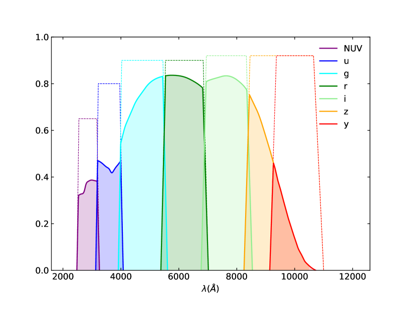
Figure 1: The CSST intrinsic transmissions (dashed) and total transmissions with detector quantum efficiency (solid) of 7 photometric filters. The details of parameters of transmissions can be found in (Cao et al. 2018) and Meng et al. (in preparation).

2 Mock Data

Mock images are generated based on the F814W band of Advanced Camera for Surveys of Hubble Space Telescope ($HST$-ACS) and COSMOS catalogs (Koekemoer et al. 2007; Massey et al. 2010; Bohlin 2016; Laigle et al. 2016). This survey has similar spatial resolution as the CSST, and background noise is $\sim 1/3$ of the CSST photometric survey. Therefore, it provides a good basis to simulate galaxy images of CSST photometric survey as real as possible. The details of image generation procedure are explained in Zhou et al. (2022) and Meng et al. (in preparation), and we summarize the important points here.

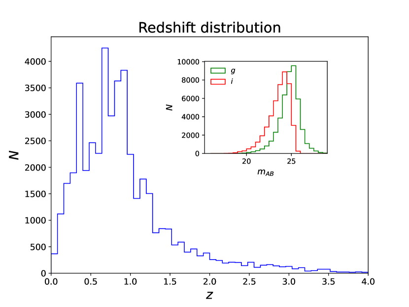
Figure 2: CSST galaxy redshift distribution derived from the COSMOS catalog. These galaxies are selected with SNR larger than 10 in $g$ or $i$ bands. The distribution peaks around $z=0.6\sim 0.7$, and can reach maximum at $z\sim 4$. We also show the distribution of AB magnitudes in the $g$ and $i$ bands.

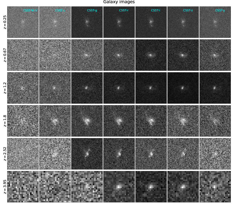
Figure 3: Examples of simulated galaxy sources in 7 CSST photometric bands at different redshifts. We notice that noises in $NUV,u$ and $y$ bands are more dominant since their transmissions are relatively low. Besides, some sources in high redshifts are almost overwhelmed by background noises in some band, and the neural network method can be applied to try to extract information in these images.

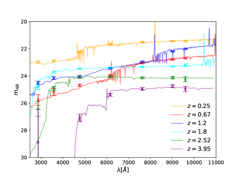
Figure 4: The corresponding fluxes of galaxy samples in Figure 3 measured by the aperture photometry method. The galaxy SEDs are also shown and rescaled to the levels of flux data for comparison.

Firstly, we select an area of $0.85\times 0.85$ deg² from the $HST$-ACS survey, where $\sim 192,000$ galaxies can be identified. Then we rescale the pixel size from $0.03$ arcsec of the $HST$ survey to $0.075$ of the CSST survey. The identified galaxies are extracted as square stamp images with galaxies at the center of images. The image sizes are 15$\times$ galaxies’ semi-major axis, which can be obtained in the COSMOS weak lensing source catalog (Leauthaud et al. 2007), so our galaxy images are in different sizes. Other sources in the image are masked and replaced by background noise, and only the galaxy image in the center is reserved.

Then we can rescale galaxy images from the $HST$-ACS F814W survey to the CSST flux level by using galaxy SEDs to obtain the CSST 7-band images. Galaxy SEDs can be produced by fitting fluxes and other photometric information given in COSMOS2015 catalog by $LePhare$ code (Laigle et al. 2016; Arnouts et al. 1999; Ilbert et al. 2006) and photo-$z$s from the catalog are fixed during the fitting procedure. The SED templates applied are also from this catalog, and we extend these templates from $\sim 900$ Å to $\sim 90$ Å using the BC03 method  (Bruzual & Charlot 2003) to include the fluxes of high-$z$ galaxies in all CSST photometric bands, where details can be found in  Cao et al. (2018). About $100,000$ high quality galaxies with reliable photo-$z$ measurement are selected. And when fitting SEDs, we also consider dust extinction and emission lines, such as Ly$\alpha$, H$\alpha$, H$\beta$, OII and OIII. After fitting the galaxy SEDs, we can calculate the theoretical flux data by convolving with the CSST filter transmissions shown in Figure 1. At the same time, fluxes of F814W images can be calculated with aperture size of 2$\times$ of Kron radius (Kron 1980). Then, the CSST 7-band images can be produced by rescaling the fluxes. The background noise also has to be adjusted to the same level of the CSST observation, and the details are given in Zhou et al. (2022). After the noise is generated, we obtain the mock CSST galaxy images for the seven CSST photometric bands.

Our galaxy flux mock data are measured by aperture photometry. We first measure the Kron radius along major and minor-axis to obtain an elliptical aperture of size $1\times R_{\rm Kron}$. Then the flux and error in each band can be calculate within this aperture. Note that the measured fluxes in some bands could be negative due to relatively large background noise. It has been proven that this effect does not affect training of our networks, and as shown later, we will rescale the fluxes and try to reserve the information.

The redshift distribution of galaxy sources selected from the COSMOS catalog are shown in Figure 2, and the selection details are explained in the next section. Commonly, we need spectroscopic redshifts as accurate redshift values to train neural networks. Here, we assume our selected galaxies can be seen as data with accurate redshifts or spec-$z$s, since we have fixed photo-$z$s from COSMOS2015 catalog in our simulation procedure. Besides, since the purpose of this work is mainly about method validation, this assumption should be reasonable currently. We can see that the distribution peaks around $z=0.6\sim 0.7$, and can reach maximum at $z\sim 4$, which is in consistency with previous studies (Cao et al. 2018; Gong et al. 2019; Zhou et al. 2021). Figure 3 shows some examples of CSST mock galaxy stamp images at different redshifts, and the corresponding SEDs of these galaxies are displayed in Figure 4. We notice that galaxies at low redshifts usually have higher SNRs with low backgrounds, contrarily, galaxies at high redshifts can be easily dominated by background noise, especially in $NUV$, $u$ and $y$ bands with low transmissions. Thus neural network is necessary to be applied for extracting information from these noisy images, and with Bayesian neural networks, uncertainties brought by background noise and the network itself can be well captured.

3 Methods

We use Bayesian MLP and Bayesian CNN to derive photo-$z$ from mock flux and image data respectively. And these two networks are combined to test the improvement of accuracy when including both data. We first briefly introduce Bayesian neural networks, and then the architectures and training process are discussed. All networks we construct are implemented by Keras with TensorFlow as backend and TensorFlow-Probability.

3.1 BNN

Generally, neural network only produces point value estimate without errors, since weights are fixed after training and the output is simply the values of parameters we are interested in. In order to correctly capture the parameter uncertainties, we have to understand where they come from. Uncertainties brought by neural network compose of two parts. One comes from instrinsic corruption of data, called aleatoric uncertainty, and this uncertainty can not be reduced in training  (Hora 1996; Kiureghian & Ditlevsen 2009).  Bishop (1994) proposed Mixture Density Network (MDN) to capture aleatoric uncertainty using mixture of distributions to replace the point estimate of networks. The output of MDN consists of the weights and parameters of each distribution, say mean $\mu$ and standard deviation $\sigma$ for Gaussian distributions. After training, we can sample from the mixture of distributions for testing data, and then calculate the uncertainty of predictions.

The other one is called epistemic uncertainty, which comes from insufficient training of network. Gathering more training data or taking average of results from ensemble networks can reduce this kind of uncertainty. Bayesian network says the weights of network can be sampled from posterior distributions learned by training data given proper priors of weights. Thus when testing, these weights vary in every run and the epistemic uncertainty can be captured with enough runs. Mathematically, we define prior of weights as $p(\omega)$ and the posterior of network weights learned from training data pair ${\mathbf{X,Y}}$ as $p(\omega|\mathbf{X,Y})$, so for test input $\mathbf{x}$, the distribution of output $\mathbf{y}$ can be calculated as:

$$p(\mathbf{y|x,X,Y})=\int p(\mathbf{y|x},\omega)p(\omega|\mathbf{X,Y})d\omega.$$ (1)

The analytical calculation of this equation is difficult, since $p(\omega|\mathbf{X,Y})$ can not be evaluated analytically. However, this distribution can be approximated by variational inference approach (Blundell et al. 2015). In variational inference, we define a variational distribution, $q(\omega)$, which has analytical form to replace $p(\omega|\mathbf{X,Y})$. The parameters of this distribution are learned so that $q(\omega)$ is as close as possible to real posterior. The approximation can be performed by minimizing their Kullback-Leibler (KL) divergence, which measures similarity between two distributions. Therefore, Equation 1 can be rewriten as:

$$p(\mathbf{y|x})\approx\int p(\mathbf{y|x},\omega)q(\omega)d\omega.$$ (2)

Minimizing KL divergence between $q(\omega)$ and $p(\omega|\mathbf{X,Y})$ is equivalent to maximizing the log-evidence lower bound (log-ELBO) (Gal & Ghahramani 2015), that is,

$$\mathcal{L}_{VI}=\int q(\omega)\log{p(\mathbf{Y|X},\omega)}d\omega-D_{\rm KL}(q(\omega)||p(\omega)),$$ (3)

where the first term is the log-likelihood of output parameters of training data, and the second term can be approximated as an $L_{2}$ regularization as shown in Gal & Ghahramani (2015). So this equation can be written as

$$\mathcal{L}_{VI}\approx\sum_{n=1}^{N}\mathcal{L}(\mathbf{y}_{n},\mathbf{\bar{y}}_{n}(\mathbf{x}_{n},\omega))-\lambda\sum_{i}|\omega_{i}|^{2},$$ (4)

where $n$ and $i$ denote number of training data and weights, respectively, and weights are sampled from $q(\omega)$. $\mathcal{L}(\mathbf{y}_{n},\mathbf{\bar{y}}_{n}(\mathbf{x}_{n},\omega))$ is the likelihood of network prediction $\mathbf{\bar{y}}_{n}(\mathbf{x}_{n},\omega)$ for input $\mathbf{x}_{n}$ with labels $\mathbf{y}_{n}$, and $\lambda$ is the regularization strength. Ignoring the regularization, minimizing KL divergence is to maximizing the log-likelihood. After training, we can perform multiple runs of testing data through network to obtain output parameters mutiple times. This procedure is identical to implementing Equation 2 to sample from variational distribution $q(\omega)$ to construct distributions of outputs, $p(\mathbf{y|x})$.

However, sampling from posterior distributions of weights only captures epistemic distributions. For regression tasks, if we assume that the predictions of parameters of a single run also obey some distributions, then we can capture the aleatoric uncertainties. Gaussian distributions are the most commonly used ones. Therefore, the log-likelihood of Equation 4 can be written as a Gaussian log-likelihood:

$$\mathcal{L}(\mathbf{y}_{n},\mathbf{\bar{y}}_{n}(\mathbf{x}_{n},\omega))=\sum_{j}\frac{-1}{2\sigma_{j}^{2}}|y_{n,j}-\bar{y}_{n,j}(\mathbf{x}_{n},\omega)|^{2}-\frac{1}{2}\log\sigma_{j}^{2},$$ (5)

where $\sigma_{j}$ represents the aleatoric uncertainties of $j$th parameters inherited from corruption of input data. $\sigma_{j}$ can be predicted along with parameters. No labels of $\sigma_{j}$ are required, since they can be produced when balancing the two terms in Equation 5. Predictions with aleatoric uncertainties can be obtained by sampling from Gaussian distributions with output parameters as means and standard deviations. Therefore, combining aleatoric and epistemic uncertainty is performing multiple runs for testing data, and in each run, predictions are sampled from Gaussian distributions.

Bayesian neural networks are built upon special layers with trainable weights, where the forms of posterior and prior distributions must be given. For simplicity, we select multivariate standard normal distribution as priors, thus the posteriors are normal distribution with learnable means and deviations. In forward pass, the network samples weights from posteriors and estimates outputs from inputs. However, backpropagation can not produce gradients of means and deviations from distributions. There is a trick to cope with this problem called re-parameterization (Kingma & Welling 2013). This trick samples $\mathbf{\epsilon}$ from a parameter-free distribution and transforms $\mathbf{\epsilon}$ with a gradient-defined function $t(\mathbf{\mu,\sigma,\epsilon})$. Commonly, $\mathbf{\epsilon}$ is sampled from a standard normal distribution, i.e, $\mathbf{\epsilon}\sim\mathcal{N}(0,\mathbf{I})$, and the function is defined as $t(\mathbf{\mu,\sigma,\epsilon})=\mathbf{\mu+\sigma\odot\epsilon}$, which shifts the $\mathbf{\epsilon}$ by mean $\mathbf{\mu}$ and scales it by $\mathbf{\sigma}$, where $\odot$ is matrix element-wise multiplication. Then the backpropagation algorithm can be accomplished. We use flipout layers introduced in Wen et al. (2018), which uses roughly twice as many floating point operations than re-parameterization layer, but can achieve significant lower variance and speedup training process.

3.2 Network Architecture

3.2.1 Bayesian MLP

Since our galaxy flux data consists of 7 discrete points obtained by 7 CSST photometric bands, we adopt MLP to predict photo-$z$ from flux data. MLP is composed of input layers, hidden layers and output layers, and the layers are connected by trainable weights and biases. The internal relationship between flux data and redshift can be learned when training. We apply DenseFlipout layer to build our Bayesian MLP.

More relevant information can give more accurate predictions, so our inputs of network are fluxes, colors and errors (Zhou et al. 2021). The fluxes and errors are typically in exponential form, and it is not suitable to directly input network, where the weights will have very large fluctuations. To speed up training and reduce fluctuations of weights, data should be normalized or rescaled. Therefore, we divide fluxes with corresponding fluxes of magnitude limits of 7 bands of CSST mentioned in Section 1. Note that our result is not sensitive to the divided values. And errors are divided with their corresponding fluxes to obtain relative errors. Since colors are values of subtraction of magnitudes between two bands, we construct color-like values as division of fluxes between two bands. There are still some large values inappropriate for networks, so we need to rescale these values with a logarithmic function. As we mentioned, since fluxes and errors are measured within apertures, some negative fluxes in bands severely affected by background noise may arise, especially in $NUV,u$ and $y$ bands. To solve this problem, we use the following logarithmic function:

$$f(x)=\left\{\begin{array}[]{lcc}\log(x)&&{x>0,}\\ -\log(-x)&&{x<0.}\\ \end{array}\right.$$ (6)

This function will rescale the fluxes, colors and errors obtained in the first rescaling, and reserve the negative information which may be useful for photo-$z$ predictions. Hereafter, we simply call the rescaled fluxes, colors and errors as fluxes, colors and errors in the context.

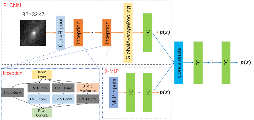
Figure 5: Architecture of our Bayesian MLP, CNN and Hybrid network. Bayesian MLP is shown in dash-dotted blue box. The inputs are fluxes, colors and errors, and 6 hidden or fully connected (FC) layers are stacked. The output is a Gaussian distribution of predicted photo-$z$. The dashed black box displays the structure of Bayesian CNN, and its input is $32\times 32\times 7$ images. The input is convolved by Convolution2DFlipout layer, and then downsampled, obtaining a feature map. Then the feature map is processed by 3 inception blocks, and the output is flattened to vector for connecting with following fully connected layer. Then the Gaussian distribution of photo-$z$ can be obtained. Inception block is illustrated in blue dashed box, where $3\times 3$ and $5\times 5$ kernels are used to extract features in different scales. Bayesian Hybrid network combines MLP and CNN by concatenating features extracted from them, and then several fully connected layers are structured to obtain the distribution of photo-$z$. Note that all layers with trainable weights are flipout layers, where the form of prior and posterior distribution must be provided, except for $1\times 1$ convolution, since this layer simply acts as a scaling one to reduce channels of features and increase computation efficiency.

Table 1: Details of Bayesian MLP architecture.

Layers	Output Statusa	Number of params.b
Input	20	0
FCc	40	1640
ReLU	40	0
FCc	40	3240
BatchNormalization	40	160d
ReLU	40	0
	…e
Params	2	162
$\mathcal{N}(\mu,\sigma)$f	-	0

Notes.
^a Number of data points or neurons.
^b Total number of parameters: 18,802.
^c FC: fully connected layer.
^d Half of them are non-trainable parameters.
^e 4 repeats of FC + BatchNormalization + ReLU.
^f Output is a Gaussian distribution with mean $\mu$ and standard deviation $\sigma$ obtained in params.

Table 2: Details of Bayesian CNN architecture.

Layers	Output Statusa	Number of params.b
Input	(32, 32, 7)	0
Convolution2DFlipout	(16, 16, 32)	4064
LeakyReLU	(16, 16, 32)	0
Inception	(8, 8, 72)	17632
Inception	(4, 4, 72)	19552
Inception	(2, 2, 72)	19552
GlobalAveragePooling	72	0
FCd	40	5800
BatchNormalization	40	160c
ReLU	40	0
Params	2	162
$\mathcal{N}(\mu,\sigma)$e	-	0

Notes.
^a Format: (dimension, dimension, channel) or number of neurons.
^b Total number of parameters: 66,922.
^c Half of them are non-trainable parameters.
^d FC: fully connected layer.
^e Output is a Gaussian distribution with mean $\mu$ and standard deviation $\sigma$ obtained in params.

Therefore, our Bayesian MLP has 20 inputs, i.e, 7 fluxes, 7 errors and 6 colors. We construct 6 hidden DenseFlipout layers with 40 units in each layer (Zhou et al. 2022), and find 6 hidden layers are proper to cope with this task. To reduce overfitting, after each layer except for the first, BatchNormalization is applied (Ioffe & Szegedy 2015), and all layers are activated by Rectified Linear Unit (ReLU) non-linear function (Nair & Hinton 2010). Bayesian MLP outputs a Gaussian distribution constructed from redshift as mean and aleatoric uncertainty as deviation. The details of architecture are shown in Table 1 and in Figure 5. Note that the parameters are approximately as twice large as non-Bayesian MLP shown in Zhou et al. (2022), since the weights are constructed by Gaussian distributions with two parameters.

3.2.2 Bayesian CNN

We use Bayesian CNN to predict photo-$z$ from CSST mock galaxy images. These images are from 7 CSST bands and can be considered as 2d-arrays with 7 channels, from which 2d Bayesian CNN can extract information to predict photo-$z$. As we mentioned in Section 2, the images are sliced according to semi-major axis of galaxies given in catalog, therefore, the final images are in different sizes. Since neural network can only process data with same sizes, we need to crop images with size larger than a threshold area $S_{\rm threshold}$ and pad images with size smaller than $S_{\rm threshold}$. Cropping is performed centrally since galaxies reside in center of images. And images are padded with typical background noise derived in Section 2 to better simulate the real observations. The most proper value of $S_{\rm threshold}$ is proven to be $32$ pixels, and other sizes $16$ and $64$ pixels are also researched. We find smaller one loses too much information since most galaxies occupy pixels larger than $16$, and the larger one introduces more background noise causing network cannot concentrate on the central galaxies.

Inception blocks proposed by Szegedy et al. (2014) can extract information in different scales parallelly and effectively combine them.  Pasquet et al. (2019) and  Henghes et al. (2021) and our previous work build their networks based on inception block to predict photometric redshift from images and achieve quite accurate results. Therefore, we construct Bayesian inception blocks with flipout layers. Our inception block is illustrated in Figure 5 and use Convolution2DFlipout layers with $3\times 3$ and $5\times 5$ kernels to extract features and learn the distributions of trainable weights. The $1\times 1$ kernels can reduce channels of features and increase computation efficiency and we do not use distributions to express the weights of these layers.

Our Bayesian CNN inputs $32\times 32\times 7$ images. The input images are firstly processed by a Convolution2DFlipout layer with $32$ kernels of $3\times 3$ size and stride size $2$ to extract information and downsample images to $16$. Following first layer is $3$ inception blocks to learn more abstract features and we finally obtain feature images with a size $2$. In order to connect with fully connected layer, we utilize global average pooling to vectorize the feature images to $72$ values (Lin et al. 2013) and employ one fully connected layer with $40$ units. The fully connected layer is also built upon DenseFlipout with learnable distribution of weights. Outputs of this network is a Gaussian distribution the same as Bayesian MLP mentioned above. Note that after each Convolution2DFlipout layer, we apply BatchNormalization layer and ReLU activation function. The details of architecture are shown in Figure 5 and Table 2. The parameters are about as twice large as non-Bayesian CNN shown in Zhou et al. (2022).

3.2.3 Bayesian Hybrid

The galaxy images in 7 bands abstractly contain fluxes, colors, errors and morphological information, which means these information can be extracted from images. And our Bayesian CNN can directly learn photo-$z$s from images, probably extracts features related to these information. In contrast, our MLP inputs the obvious flux information and fitting the relation between redshifts and flux data. Hence, if we combine MLP and CNN to construct a hybrid network and this network can input both flux data and images, it may result in more accurate photo-$z$ predictions. We construct hybrid network by concatenating Bayesian MLP and CNN mentioned above in both last fully connected layer, obtaining a vector of size $80$, and then structure $6$ fully connected layers with $80$ units built upon DenseFlipout to learn distribution of weights. And after each layer, BatchNormalization and ReLU activation function are applied. The output of this hybrid network is the same as Bayesian MLP and CNN mentioned above. The schematic diagram is illustrated in Figure 5.

3.3 Training

Here, we follow Zhou et al. (2022) and select about $40,000$ high-quality sources with SNR in $g$ or $i$ band larger than $10$ from generated dataset mentioned in Section 2. These sources all possess both flux data and images. As we notice, we consider their reliable photo-$z$s as accurate spectroscopic redshifts that can be used in our training process. And in the real CSST survey, samples with spec-$z$ obtained by future deep spectroscopic surveys will be used to retrain our networks. The above samples are divided into training and testing sets. We spare $10,000$ samples for testing and the rest, about $30,000$ are used for training, constructing a ratio of training to testing to be approximately $3:\ 1$. And we split 10% for validation from training data. We also try $1:\ 1$ and $1:\ 3$ ratio to study the influence of training size on accuracy of photo-$z$.

Our Bayesian MLP uses the negative of Gaussian log-likehood (negative of Equation 5) as our loss function, which considers both aleatoric and epistemic uncertainties. The Adam optimizer is adopted to optimize weights of the network. This optimizer can adjust learning rate of every weight automatically given an initial learning rate, which is set to be $10^{-4}$ for this network. We create an accuracy metric based on the definition of outlier percentage to be $|z_{\rm true}-z_{\rm pred}|/(1+z_{\rm true})<0.15$. Note that this metric cannot represent the final result, since the $z_{\rm pred}$ is a random draw from learned distribution of photo-$z$. This accuracy metric is monitored in training as well as negative log-likelihood loss. The maximum number of epoch and batch size in each epoch are set to be $2000$ and $2048$, respectively. In order to reduce the statistical noise and create more data, we augment training data by random realizations based on flux errors with Gaussian distribution (Zhou et al. 2022). Here $50$ realizations are created and more realizations cannot significantly improve the results. In training, we notice that the validation accuracy and loss follow the training ones well, and no overfitting occurs.

Our Bayesian CNN uses the same loss function and optimizer. The initial learning rate is also set to be $10^{-4}$. The maximum number of epoch is also $2000$. Batch size in every epoch is set to be $1024$. We save the model when validation loss and accuracy are converged. We augment training data by including their rotated and flipped counterparts, resulting a $8\times$ data size. This augmentation can probably make the network more accustomed to background noise and better concentrate on central galaxies.

Bayesian hybrid network uses the same setting of loss and optimizer. The maximum number of epoch and batch size is $2000$ and $512$ and the converged model with steady validation loss and accuracy is saved as our final model. The inputs of MLP part are augmented by $50$ random realizations based on errors, and the images are randomly rotated or flipped to correspond one specific realization of flux data. Thus the network can reduce the statistical noise brought by flux data, and can be accustomed to background noise at the same time.

Since Bayesian MLP and CNN can predict photo-$z$ accurately, the features learned by the two networks are optimized to fullfill this task. To explore if further improvement exists for photo-$z$, we try to investigate that if the features learned by both CNN and MLP are better than features directly learned by hybrid network. We create a hybrid transfer network, inspired by the techniques from transfer learning (TL), which utilizes existing knowledge from one problem to solve related problem (Pan & Yang 2009). The MLP and CNN parts of this network is transferred from trained ones and their weights are frozen. Thus the features combined by this network are the ones already learned by MLP and CNN, respectively, instead of directly learned by the hybrid network. Note that the structure of this network is the same as the hybrid one, except for employing a new training strategy from transfer learning. In training, we find freezing the layers before the last fully connected layers of MLP and CNN to include more flexibility result better.

3.4 Calibration

The uncertainties predicted by neural network are probably miscalibrated (Guo et al. 2017; Ovadia et al. 2019). We can examine if our network is well calibrated through reliability diagram, which shows the coverage probability of samples with true values residing in specific confidence interval. If the true values of $x\%$ samples lies in $x\%$ confidence interval, then this network model is well calibrated (Perreault Levasseur et al. 2017; Hortúa et al. 2020) and the reliability diagram should be a straight diagonal line.

The calibration can be achieved by tuning hyper-parameters of networks when training, such as the kernel size for convolution layer, regularization parameters and so on. However, fine-tuning hyper-parameters is a challenging and time-consuming task. Calibration after training is also an option and the relevant methods are described in literature (see references in Hortúa et al. (2020)). We use Beta calibration introduced in Kull et al. (2017). Firstly, we construct the reliability diagram for testing data and use following function to fit this line:

$$\beta(x;a,b,c)=\frac{1}{1+1/(e^{c}\frac{x^{a}}{(1-x)^{b}})}$$ (7)

where $a,b$ and $c$ are the fitting parameters. We scale covariance matrix $\Sigma$ by a factor $s$ to obtain $s\Sigma$, and choose the $s$ parameter for minimizing the difference between the fitting line and diagonal line. Therefore, $s\Sigma$ is a well calibrated covariance matrix. For our photo-$z$ work, we just need to scale the uncertainty of every sample.

4 Results and Discussions

The percentage of catastrophic outliers is widely used in photo-$z$ research. Here, we define our catastrophic outliers to be $|\delta z|/(1+z_{\rm true})<0.15$, where $\delta z=z_{\rm pred}-z_{\rm true}$. The normalized median absolute deviation is another mainly adopted quantity, which can be calculated as

$$\sigma_{\rm NMAD}=1.48\times{\rm median}\left(\left|\frac{\delta z-{\rm median}(\delta z)}{1+z_{\rm true}}\right|\right).$$ (8)

This deviation shows the scattering of predictions considering the evolution of redshift, and provides a proper estimation of accuracy. The average of $|\delta z|/(1+z_{\rm true})$ as MAE is also calculated for comparison with literature. Besides, to measure the performance of confidence, we calculate the average 1$\sigma$ photo-$z$ uncertainties $\overline{E}$ in the predictions. And we define a similar metric called coverage introduced in Jones et al. (2022) to examine our reliability of uncertainties:

$$C=\sum_{i}^{N_{gal}}\frac{|\overline{z}_{{\rm pred},i}-z_{{\rm true},i}|<\sigma_{i}}{N_{gal}}$$ (9)

where $N_{gal}$ is the number of galaxy samples in specific redshift bin, and $\sigma$ is the 68% confidence interval of prediction for every sample. After feeding testing data to our four networks, we calibrate these models with the method mentioned in Section 3.4 and plot a reliability diagram in Figure 6. Notice that they are well calibrated and the scaling parameters are close to 1, which means that they are almost self-calibrated when training.

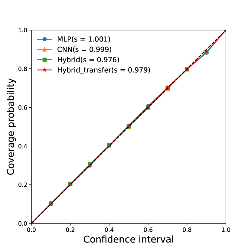
Figure 6: The reliability diagram for four networks. The uncertainties predicted by four networks are reliable when calibrated after Beta calibration method.

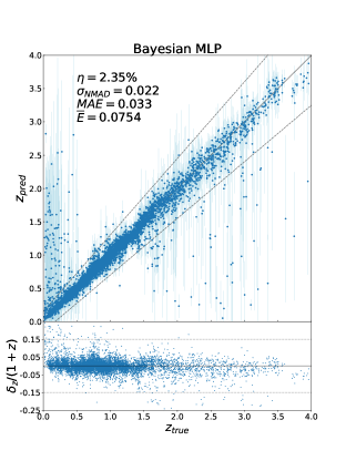
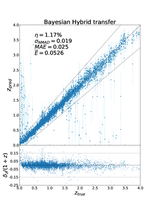
Figure 7: Photo-$z$ result of Bayesian MLP, CNN, hybrid and hybrid transfer networks. The $\eta,\sigma_{\rm NMAD}$ and $\overline{E}$ represents the outlier fraction, normalized median absolute deviation, and average 1$\sigma$ uncertainties or errors, respectively. The error bars are derived from the Gaussian distributions output by the networks. Hybrid and hybrid transfer networks can achieve outlier fraction smaller than 1.5% and $\sigma_{\rm NMAD}\simeq 0.02$.

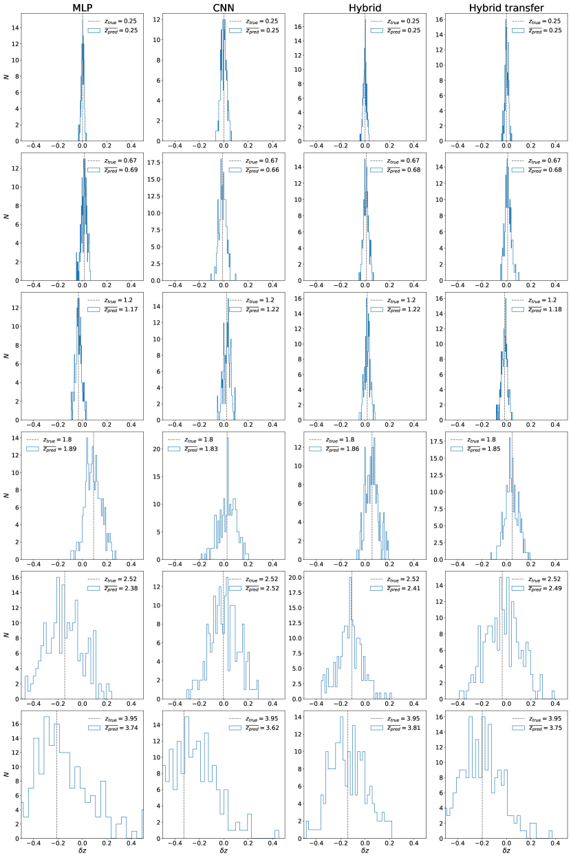
Figure 8: PDFs for the deviations of predicted and true redshifts, provided by the Bayesian MLP, CNN, hybrid and hybrid transfer network for the galaxy samples shown in Figure 3. Dashed lines show the deviations of average predictions to the true redshifts.

Figure 9: The distributions of photo-$z$ uncertainties for the four networks. Most uncertainties are lower than 0.2, but the ones of MLP can be higher, reaching a maximum at about 1.5.

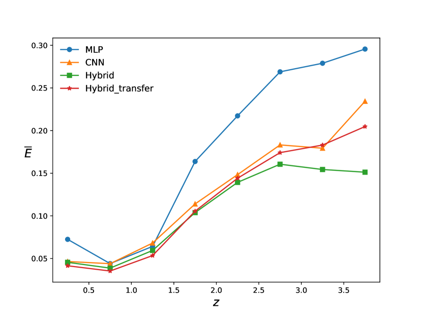
Figure 10: The average photo-$z$ uncertainties in different redshift bins. The four networks perform similarly well in redshift range $0.5\sim 1.5$, assuring accuracy and confidence for most of galaxies.

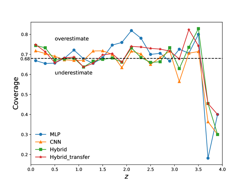
Figure 11: The coverage of photo-$z$ predictions. We notice that our curves fluctuate around 0.68 in low redshifts, and the fluctuations become larger at higher redshifts. Uncertainties of samples with $3.5<z<4.0$ are highly underestimated, probably resulting from statistical variance with few samples.

We show the photo-$z$ result for Bayesian MLP using the flux mock data in the upper-left panel of Figure 7, finding that the outlier fraction is 2.35% and $\sigma_{\rm NMAD}$ is 0.022 for testing data. The outlier fraction is higher than the estimation ($\sim 1.4\%$) using the normal MLP in Zhou et al. (2022), since much larger number of trainable parameters are included in the Bayesian MLP which are probably more difficult to optimize and suppress the prediction accuracy. Maybe the price of obtaining the uncertainties of predictions is worse performance in point estimate. However, we obtain similar $\sigma_{\rm NMAD}$ as  Zhou et al. (2022), meaning the dispersion of predictions is at the same level. The error bars are large for some samples with redshift lower than $0.5$ and larger than $1.5$, meaning that network cannot predict these redshift well and assign them with very high uncertainty. However in $0.5<z<1.5$, the outlier fraction and uncertainties are much lower, assuring high accuracy and confidence for most of galaxies observed by CSST. This feature is probably due to the number of training data used at different redshifts, that most galaxies in the training sample are within $0.5<z<1.5$ (see Fig. 2).

The upper-right panel of Figure 7 shows the result from Bayesian CNN using galaxy images. We find that the Bayesian CNN can achieve outlier fraction 1.32% and $\sigma_{\rm NMAD}=0.022$. The outlier fraction is better than the MLP result. Since images should abstractly include both morphological and flux information, in principle, the CNN could potentially extract all of these information, and provide comparable or even better predictions than the MLP using the flux information only.

Lower panels of Figure 7 shows the result of Bayesian hybrid and hybrid transfer result, respectively. The outlier fraction and $\sigma_{\rm NMAD}$ are 1.23% and 0.021, and 1.17% and 0.019 for the two networks. We can see that combining flux data and galaxy images can further decrease the outlier fraction. And the one employing transfer learning provides slightly better result, implying features from trained MLP and CNN are probably more proper than features directly learned by the hybrid network. The performance by hybrid and hybrid transfer networks are obviously better than the MLP and CNN, which means that properly including both morphological and flux information can improve photo-$z$ predictions.

Figure 8 displays the PDFs for the deviation of predicted and true redshifts, provided by the Bayesian MLP, CNN, hybrid and hybrid transfer networks, respectively, for the galaxy samples given in Figure 3. Dashed lines show the deviations of average photo-$z$ predictions to the true redshifts. We notice that at high redshift, the results are highly deviated from 0 and the PDFs are much wider, resulting less confident predictions.

Figure 9 shows the distributions of predicted photo-$z$ uncertainties for the four networks. We notice that most uncertainties stay below 0.2, but the ones of MLP can be higher, reaching a maximum at about 1.5. We also show the average photo-$z$ uncertainties $\overline{E}$ in different redshift bins in Figure 10. Here the bin size we use is 0.5. The uncertainties for the four networks in redshift range from 0.5 to 1.5 are similarly small, assuring the accuracy for most galaxies. The MLP are relatively higher in the whole redshift range, explaining the messy plot in upper-left panel in Figure 7. The uncertainties of CNN, hybrid and hybrid transfer networks are suppressed compared to the MLP case, and hybrid transfer achieves the lowest uncertainties in low redshifts where most galaxies reside, but hybrid succeed in higher redshifts. We calculate the average photo-$z$ uncertainties $\overline{E}$ for the whole range, and we have $\overline{E}$ = 0.754, 0.0611, 0.0552 and 0.0526 for Bayesian MLP, CNN, hybrid and hybrid transfer networks, respectively. We note that the hybrid and hybrid transfer networks result in similar average uncertainties, and hybrid transfer performs slightly better.

We also plot the “coverage” metric originally defined in Jones et al. (2022), which examines reliability of uncertainties with redshifts. In Figure 11. We notice our curves fluctuate around 0.68 in low redshifts and the fluctuations become larger at higher redshifts. Uncertainties of samples with $3.5<z<4.0$ are highly underestimated, probably resulting from statistical variance with few samples.

Table 3: Result comparison for our networks trained with different training data size.

Train size(train-test ratio)	statistics	MLP	CNN	Hybrid	Hybrid transfer
30,000 (3: 1)	$\sigma_{\rm NMAD}$	0.022	0.022	0.021	0.019
	$\eta$	2.35%	1.32%	1.23%	1.17%
	$\overline{E}$	0.0754	0.0611	0.0552	0.0526
20,000 (1: 1)	$\sigma_{\rm NMAD}$	0.022	0.022	0.021	0.019
	$\eta$	2.48%	1.64%	1.41%	1.28%
	$\overline{E}$	0.0758	0.0594	0.0578	0.0532
10,000 (1: 3)	$\sigma_{\rm NMAD}$	0.023	0.024	0.023	0.021
	$\eta$	2.43%	1.81%	1.67%	1.44%
	$\overline{E}$	0.0794	0.0656	0.0610	0.0551

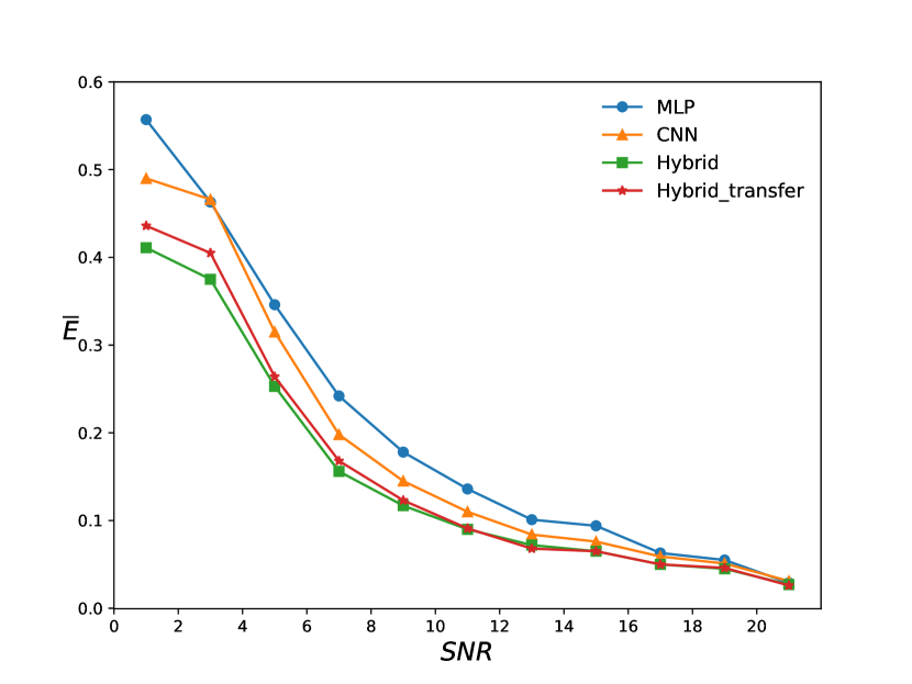
Figure 12: The relation of average uncertainties and SNR. We notice that as expected, the average uncertainties decrease when the SNRs become larger, and hybrid and hybrid transfer networks perform better than MLP and CNN case.

Note that the results above are analyzed based on a training sample with $\sim$30,000 galaxies (a training and testing ratio of about $3:\ 1$ in our case). We also test if the performance of the four networks will be severely affected when feeding smaller set of training data, since we probably do not have large number of high quality photometric samples with spectroscopic redshifts in real observations. Here, we split the data so that the training data are about 20,000 (train-test ratio of $3:\ 1$) and 10,000 (train-test ratio of $1:\ 3$) to retrain these networks and calculate the results, which is shown in Table 3. And the calibration scale parameters $s$ are 0.998, 0.963, 1.140, 1.048 and 1.105, 0.935, 1.370, 0.882 for MLP, CNN, hybrid and hybrid transfer networks trained with 20,000 and 10,000 data respectively. Decreasing training data does not provide severely worse results. We notice that MLP even improves its outlier percentage from 20,000 to 10,000, probably because 10,000 training data is enough for training of MLP. The hybrid transfer network is robust to decreasing of training data, providing similarly confident predictions.

In order to investigate the relationship between the SNR and uncertainties of photo-$z$, we select data with SNR in $g$ or $i$ band larger than 1, sparing 20,000 for testing, and retrain all networks. We show the average uncertainty as a function of the SNR in Figure 12. We notice that the uncertainties decrease with SNR growing as expected, and the hybrid and hybrid transfer networks perform better than the MLP and CNN case. Hybrid transfer results are worse in lower SNR, probably because of the influence of transferred MLP and CNN parts, and they reach similar level when the SNR is larger than 10. The last points converge because they are calculated for samples with SNR$>$20.

5 Conclusion

In this work, we use Bayesian neural networks to explore the photo-$z$ accuracy and uncertainty for the CSST photometric survey. The CSST data is simulated based on the COSMOS catalogs. Here we use four networks, including Bayesian MLP, CNN, hybrid and hybrid transfer networks. The Bayesian framework is built upon variational inference technique, so that the weights are posterior distributions learned from given prior and training data. The distributions of weights account for epistemic uncertainty, which comes from insufficient training and lack of data. On the other hand, the aleatoric uncertainty coming from intrinsic corruption of data also needs to consider.

Bayesian MLP inputs flux data, including flux, color and error. These inputs are all rescaled to proper value range to speed up the training process. Bayesian CNN processes galaxy images from the seven CSST bands. Our CNN is built upon inception blocks, which can extract information in different scales and is beneficial for predicting photo-$z$. Bayesian hybrid and hybrid transfer network are combinations of MLP and CNN through their learned features. The hybrid transfer network shares the same architecture with the hybrid networks, but applies a different training strategy borrowed from transfer learning. This hybrid transfer network freezes the weights of MLP and CNN parts transferred from trained ones, and only the latter layers are optimized.

We find that all of these networks can derive accurate photo-$z$ results and use calibration method to obtain reliable uncertainties of predictions. CNN can provide lower outlier fraction and more confident predictions than the MLP, indicating CNN is capable to extract more information from the images besides the flux data. The hybrid and hybrid transfer networks result in similar performance with the hybrid transfer slightly outperforming in outlier fraction and average photo-$z$ uncertainty. This result shows that feeding network with both flux data and images can improve the photo-$z$ predictions. We also explore the effect of decreasing training samples, finding that smaller samples do not severely corrupt the predictions in our case. The relationship between SNR and uncertainties of photo-$z$ is studied, and as expected, the average uncertainties decrease with SNR increasing.

We also should note that the BNNs actually need more optimization and are more time-consuming compared to traditional neural networks, since the BNNs usually have more tunable weights and the training process is more complex. However, as our work indicates, the BNNs are quite suitable and useful in photo-$z$ estimation that can obtain reliable uncertainties and PDFs with similar photo-$z$ accuracy as traditional neural networks. This means that the BNN should be a powerful tool and has large potentials to be applied in astronomical and cosmological studies.