Data Assimilation in Operator Algebras

Abstract

We develop an algebraic framework for sequential data assimilation of partially observed dynamical systems. In this framework, Bayesian data assimilation is embedded in a non-abelian operator algebra, which provides a representation of observables by multiplication operators and probability densities by density operators (quantum states). In the algebraic approach, the forecast step of data assimilation is represented by a quantum operation induced by the Koopman operator of the dynamical system. Moreover, the analysis step is described by a quantum effect, which generalizes the Bayesian observational update rule. Projecting this formulation to finite-dimensional matrix algebras leads to new computational data assimilation schemes that are (i) automatically positivity-preserving; and (ii) amenable to consistent data-driven approximation using kernel methods for machine learning. Moreover, these methods are natural candidates for implementation on quantum computers. Applications to data assimilation of the Lorenz 96 multiscale system and the El Niño Southern Oscillation in a climate model show promising results in terms of forecast skill and uncertainty quantification.

1 Introduction

Since its inception in weather forecasting [12] and object tracking problems [30], sequential data assimilation, also known as filtering, has evolved into an indispensable tool in forecasting and uncertainty quantification of dynamical systems [39, 35]. In its essence, data assimilation is a Bayesian inference theory: Knowledge about the state of the system at time $t$ is described by a probability distribution $p_{t}$. The system dynamics acts on probability distributions, carrying along $p_{t}$ to a time-dependent family of distributions $p_{t,\tau}$, which can be used to forecast observables of the system at time $t+\tau$, $\tau\geq 0$. When an observation is made, at time $t+\Delta t$, the forecast distribution $p_{t,\Delta t}$ is updated in an analysis step using Bayes’ theorem to a posterior distribution $p_{t+\Delta t}$, and the cycle is repeated.

In real-world applications, the Bayesian theoretical “gold standard” is seldom feasible to employ due to a variety of challenges, including high-dimensional nonlinear dynamics, nonlinear observation modalities, and model error. Weather and climate dynamics [31] represent a classical application domain where these challenges are prevalent due to the extremely large number of active degrees of freedom (which necessitates making dynamical approximations such as subgrid-scale parameterization) and nonlinear equations of motion and observation functions (which prevent direct application of Bayes’ theorem). Addressing these issues has stimulated the creation of a broad range of data assimilation techniques, including variational [2], ensemble [32], and particle [47] methods.

In this paper, we examine Bayesian data assimilation and its representation through finite-dimensional computational methods from a new algebraic perspective. Our formulation employs different levels of description, depicted schematically in Fig. 1. We begin by assigning to a measure-preserving dynamical flow $\Phi^{t}:X\to X$, $t\in\mathbb{R}$, an algebra of observables (complex-valued functions of the state) $\mathfrak{A}=L^{\infty}(X,\mu)$, where $X$ is the state space and $\mu$ the invariant measure. This algebra is a commutative, or abelian, von Neumann algebra [45] under pointwise function multiplication. The state space of $\mathfrak{A}$, denoted as $S(\mathfrak{A})$, is the set of continuous linear functionals $\omega:\mathfrak{A}\to\mathbb{C}$, satisfying the positivity condition $\omega(f^{*}f)\geq 0$ for all $f\in\mathfrak{A}$ and the normalization condition $\omega\bm{1}=1$. Here, ^∗ denotes the complex conjugation of functions, and $\bm{1}$ is the unit of $\mathfrak{A}$, $\bm{1}(x)=1$ for all $x\in X$. Every probability density $p\in L^{1}(X,\mu)\equiv\mathfrak{A}_{*}$ induces a state $\omega_{p}\in S(\mathfrak{A})$ that acts on $\mathfrak{A}$ as an expectation functional, $\omega_{p}f=\int_{X}fp\,d\mu$. Such states $\omega_{p}$ constitute the set of normal states of $\mathfrak{A}$, denoted as $S_{*}(\mathfrak{A})$.

Figure 1: Schematic representation of the abelian and non-abelian formulations of sequential data assimilation (DA), showing a forecast–analysis cycle. The top row of the diagram shows the dynamical flow $\Phi^{t}:X\to X$. The second row shows the observation map $h:X\to Y$ used to update the state of the DA system in the analysis step. The rows labeled , , and  show the abelian, infinite-dimensional non-abelian (quantum mechanical), and finite-dimensional non-abelian (matrix mechanical) DA systems, respectively. In , the forecast step is carried out by the transfer operator $P^{t}:S_{*}(\mathfrak{A})\to S_{*}(\mathfrak{A})$ acting on states of the abelian algebra $\mathfrak{A}$. The analysis step (blue dot) is represented by an effect-valued map $F:Y\to\mathfrak{A}$ that updates the state given observations in $Y$. In , the forecast step is carried out by the transfer operator $\mathcal{P}^{t}:S_{*}(\mathfrak{B})\to S_{*}(\mathfrak{B})$ acting on states of the non-abelian operator algebra $\mathfrak{B}$. The analysis step (red dot) is carried out by an effect $\mathcal{F}:Y\to\mathfrak{B}$ given by the composition of $F$ with the regular representation $\pi$ of $\mathfrak{A}$ into $\mathfrak{B}$ (red arrow). The state space $S_{*}(\mathfrak{A})$ is embedded into $S_{*}(\mathfrak{B})$ by means of a map $\Gamma$ which is compatible with both forecast and analysis; see (4) and (9). This compatibility is represented by the commutative loops between  and  having $\Gamma$ as a vertical arrow. To arrive at the matrix mechanical DA, , we project $\mathfrak{B}$ into an $L^{2}$-dimensional operator algebra $\mathfrak{B}_{L}$ using a positivity-preserving projection $\bm{\Pi}_{L}$. The composition of this projection with $\mathcal{F}$ leads to an effect $\mathcal{F}_{L}:Y\to\mathfrak{B}_{L}$ employed in the analysis step (purple arrow and dot). Moreover, $\bm{\Pi}_{L}$ induces a state space projection $\bm{\Pi}^{\prime}_{L}:S_{*}(\mathfrak{B})\to S_{*}(\mathfrak{B}_{L})$ and a projected transfer operator $\mathcal{P}_{L}^{(t)}:S_{*}(\mathfrak{B}_{L})\to S_{*}(\mathfrak{B}_{L})$ employed in the forecast step. Vertical dotted arrows indicate asymptotically commutative relationships that hold as $L\to\infty$.

The next level of our framework, labeled  in Fig. 1, generalizes data assimilation by embedding it in a non-abelian operator algebra. Operator algebras form the mathematical backbone of quantum mechanics [17]—one of the most successful theories in physics. Quantum information theory and quantum probability provide a unified mathematical framework to characterize the properties of information transfer in both abelian and non-abelian systems through maps (quantum operations) acting on elements of the algebra and the corresponding states [1, 27, 52]. Our non-abelian formulation  is based on the von Neumann algebra $\mathfrak{B}\equiv B(H)$ of bounded operators on the Hilbert space $H=L^{2}(X,\mu)$, equipped with operator composition as the algebraic product. The state space $S(\mathfrak{B})$ is defined as the space of continuous, positive, normalized functionals analogously to $S(\mathfrak{A})$; that is, every state $\omega\in S(\mathfrak{B})$ satisfies $\omega(A^{*}A)\geq 0$ and $\omega I=1$, where ^∗ denotes the operator adjoint on $B(H)$ and $I$ is the identity operator. Analogously to $\mathfrak{A}$, $S(\mathfrak{B})$ has a subset of normal states, $S_{*}(\mathfrak{B})$, induced in this case by trace-class operators. Specifically, letting $\mathfrak{B}_{*}\equiv B_{1}(H)$ denote the space of trace-class operators in $B(H)$, every positive operator $\rho\in\mathfrak{B}_{*}$ of unit trace induces a state $\omega_{\rho}\in S_{*}(\mathfrak{B})$ such that $\omega_{\rho}A=\operatorname{tr}(\rho A)$. Such operators $\rho$ are called density operators, and can be thought of as non-abelian analogs of probability densities $p\in\mathfrak{A}_{*}$. As we will see below, analogs of the transfer operator and Bayesian update described above for $S_{*}(\mathfrak{A})$ are naturally defined for $S_{*}(\mathfrak{B})$.

To arrive at a practical data assimilation algorithm, we project (discretize) the infinite-dimensional system on $\mathfrak{B}$ to a system on a finite-dimensional subalgebra $\mathfrak{B}_{L}\subset\mathfrak{B}$, which is concretely represented by an $L\times L$ matrix algebra (see  in Fig. 1). We show that this approach naturally leads to computational techniques which are well-suited for assimilation of high-dimensional observables, while enjoying structure-preservation properties that cannot be obtained from finite-dimensional projections of abelian formulations. Moreover, by virtue of being rooted entirely in linear operator theory, these methods are amenable to a consistent data-driven formulation using kernel methods for machine learning.

1.1 Previous work

Recently, an operator-theoretic framework for data assimilation, called quantum mechanical data assimilation (QMDA) [21], was developed using ideas from Koopman operator theory [34, 16] in conjunction with the Dirac-von Neumann axioms of quantum dynamics and measurement [46]. In QMDA, the state of the data assimilation system is a density operator $\rho_{t}$ acting on $H=L^{2}(X,\mu)$ (rather than a probability density $p_{t}\in L^{1}(X,\mu)$ as in classical data assimilation), and the assimilated observables are multiplication operators in $B(H)$ (rather than functions in $L^{\infty}(X,\mu)$). Between observations, $\rho_{t}$ evolves under the induced action of the transfer operator, and the forecast distribution of observables is obtained as a quantum mechanical expectation with respect to $\rho_{t}$. Upon making an observation, the density operator $\rho_{t}$ is updated projectively as a von Neumann measurement, which is the quantum mechanical analog of Bayes’ rule. Using kernel methods for Koopman operator approximation [24, 20, 13], QMDA has a data-driven formulation, which was shown to perform well in low-dimensional applications.

1.2 Contributions

We provide a general algebraic framework that encompasses classical data assimilation and QMDA as particular instances (abelian and non-abelian, respectively). The principal distinguishing aspects of this framework are as follows.

1. Dynamical consistency. We employ a dynamically consistent embedding of abelian data assimilation  into the non-abelian framework . As in ref. [21], observables in $\mathfrak{A}$ are mapped into multiplication operators in $\mathfrak{B}$, but here we also employ an embedding $\Gamma:S_{*}(\mathfrak{A})\to S_{*}(\mathfrak{B})$ that is compatible with the transfer operators on $S_{*}(\mathfrak{A})$ and $S_{*}(\mathfrak{B})$ (see the commutative loops between  and  in Fig. 1). This allows us to study QMDA in relation to the underlying classical theory, and establish the consistency between the two approaches.

2. Effect system. In both the abelian and non-abelian settings, the analysis step given observations in a space $Y$ acquired through an observation map $h:X\to Y$ is carried out using quantum effects (loosely speaking, algebra-valued logical predicates) [1]. In the abelian case, the effect $F:Y\to\mathfrak{A}$ is induced by a kernel feature map. In the non-abelian setting, $F$ is promoted to an operator-valued feature map $\mathcal{F}:Y\to\mathfrak{B}$; see the column in the schematic of Fig. 1 labeled “Analysis”. Our use of feature maps enables assimilation of data of arbitrarily large dimension, overcoming an important limitation of the original QMDA scheme [21] (which becomes prohibitively expensive for high-dimensional observation maps).

3. Positivity-preserving discretization. The discretization procedure leading to the finite-dimensional scheme   has the important property that positive elements of $\mathfrak{B}$ are mapped into positive elements of $\mathfrak{B}_{L}$. Moreover, the transfer operator on $S_{*}(\mathfrak{B})$ is mapped into a completely positive, trace-non-increasing map, so the finite-dimensional data assimilation system is a quantum operation. We call this system “matrix mechanical”. By virtue of these properties, the matrix mechanical system preserves the sign of sign-definite observables of the original system. Relevant examples include positive physical quantities such as mass and temperature, but also statistical quantities such as probability density which are useful for uncertainty quantification. We emphasize that the approach of first embedding classical data assimilation in $\mathfrak{A}$ to the non-abelian operator setting of $\mathfrak{B}$ and then projecting to the finite-dimensional system on $\mathfrak{B}_{L}$ is important in ensuring positivity preservation.

4. Data-driven formulation. The matrix mechanical system  admits a data-driven approximation in which all operators are represented in a kernel eigenbasis learned from time-ordered training data, without requiring a priori knowledge of the equations of motion. In the limit of large training data, the predictions made by the data-driven data assimilation system converge to those made by the system on $\mathfrak{B}_{L}$, which in turn converge to the infinite-dimensional system  on $\mathfrak{B}$ as $L\to\infty$.

5. Route to quantum computing. The matrix mechanical scheme is well-suited for implementation on a quantum computer. Previous work [23] has shown that Koopman operators of measure-preserving ergodic dynamical systems can be approximated using shallow quantum circuits, offering an exponential computational advantage over classical deterministic algorithms for Koopman operator approximation. Our approach provides a novel route to quantum algorithms that sequentially alternate between unitary evolution and projective measurement to perform inference and prediction of classical dynamics with quantum computers.

2 Embedding data-assimilation in operator algebras

Consider a dynamical flow $\Phi^{t}:X\to X$, $t\in\mathbb{R}$, on a completely metrizable, separable space $X$ with an ergodic, invariant, Borel probability measure $\mu$. The flow induces Koopman operators $U^{t}:f\mapsto f\circ\Phi^{t}$, which are isomorphisms of the $L^{p}(X,\mu)$ spaces with $p\in[1,\infty]$. The flow also induces transfer operators $P^{t}:L^{p}(X,\mu)^{*}\to L^{p}(X,\mu)^{*}$ on the dual spaces $L^{p}(X,\mu)^{*}$ of $L^{p}(X,\mu)$, given by the adjoint of the Koopman operator, $P^{t}\gamma=\gamma\circ U^{t}$. Under the canonical identification of $L^{p}(X,\mu)^{*}$, $p\in[1,\infty)$, with finite, complex Borel measures $\gamma$ with densities in $L^{q}(X,\mu)$, $\frac{1}{p}+\frac{1}{q}=1$, the transfer operator is identified with the inverse Koopman operator; that is, for $\gamma\in L^{p}(X,\mu)^{*}$ with density $\varrho=\frac{d\gamma}{d\mu}\in L^{q}(X,\mu)$, $\gamma_{t}:=P^{t}\gamma$ has density $\varrho_{t}=\frac{d\gamma_{t}}{d\mu}\in L^{q}(X,\mu)$ with $\varrho_{t}=U^{-t}\varrho$. In what follows, $\lVert f\rVert_{L^{p}(X,\mu)}=(\int_{X}\lvert f\rvert^{p}\,d\mu)^{1/p}$ and $\lVert f\rVert_{L^{\infty}(X,\mu)}=\lim_{p\to\infty}\lVert f\rVert_{L^{p}(X,\mu)}$ denote the standard $L^{p}(X,\mu)$ norms for $p\in[1,\infty)$ and $p=\infty$, respectively.

Among the $L^{p}(X,\mu)$ spaces, $H:=L^{2}(X,\mu)$ is a Hilbert space and $\mathfrak{A}:=L^{\infty}(X,\mu)$ is an abelian von Neumann algebra with respect to function multiplication and complex conjugation. In particular, for any two elements $f,g\in\mathfrak{A}$ we have

(1) $$\lVert fg\rVert_{\mathfrak{A}}\leq\lVert f\rVert_{\mathfrak{A}}\lVert g\rVert_{\mathfrak{A}},\quad\lVert f^{*}f\rVert_{\mathfrak{A}}=\lVert f\rVert^{2}_{\mathfrak{A}},$$

making $\mathfrak{A}$ a $C^{*}$-algebra, and in addition $\mathfrak{A}$ has a predual $\mathfrak{A}_{*}:=L^{1}(X,\mu)$ (i.e., a Banach space for which $\mathfrak{A}$ is the dual), making it a von Neumann algebra. We let $\langle f,g\rangle=\int_{X}f^{*}g\,d\mu$ denote the inner product on $H$. On $H$, the Koopman operator $U^{t}$ is unitary, $U^{t*}=U^{-t}$.

2.1 Embedding observables

Let $\mathfrak{B}:=B(H)$ be the space of bounded operators on $H$, equipped with the operator norm, $\lVert A\rVert_{\mathfrak{B}}=\sup_{f\in H}\frac{\lVert Af\rVert_{H}}{\lVert f\rVert_{H}}$. This space is a non-abelian von Neumann algebra with respect to composition and adjoint of operators. That is, for any two operators $A,B\in\mathfrak{B}$ we have

$$\lVert AB\rVert_{\mathfrak{B}}\leq\lVert A\rVert_{\mathfrak{B}}\lVert B\rVert_{\mathfrak{B}},\quad\lVert A^{*}A\rVert_{\mathfrak{B}}=\lVert A\rVert^{2}_{\mathfrak{B}},$$

which is the non-abelian analog of (1) making $\mathfrak{B}$ a $C^{*}$-algebra. Moreover, $\mathfrak{B}$ has a predual, $\mathfrak{B}_{*}:=B_{1}(H)$, making it a von Neumann algebra. Here, $B_{1}(H)\subseteq B(H)$ is the space of trace-class operators on $H$, equipped with the trace norm, $\lVert A\rVert_{1}:=\operatorname{tr}\sqrt{A^{*}A}$, which can be thought of as a non-abelian analog of $L^{1}(X,\mu)$. The unitary group of Koopman operators $U^{t}$ on $H$ induces a unitary group $\mathcal{U}^{t}:\mathfrak{B}\to\mathfrak{B}$ (i.e., a group of linear maps mapping unitary operators to unitary operators), which acts by conjugation, i.e.,

(2) $$\mathcal{U}^{t}A=U^{t}AU^{t*}.$$

The abelian algebra $\mathfrak{A}$ embeds isometrically into $\mathfrak{B}$ through the map $\pi:\mathfrak{A}\to\mathfrak{B}$, such that $\pi f$ is the multiplication operator by $f$, $(\pi f)g=fg$. This map is injective, and satisfies $\pi(fg)=(\pi f)(\pi g)$, $\pi(f^{*})=(\pi f)^{*}$ for all $f,g\in\mathfrak{A}$. Thus, $\pi$ is a ^∗-representation, preserving the von Neumann algebra structure of $\mathfrak{A}$. The representation $\pi$ is also compatible with Koopman evolution, in the sense that $\mathcal{U}^{t}\circ\pi=\pi\circ U^{t}$ holds for all $t\in\mathbb{R}$. Equivalently, we have the commutative diagram

$$\leavevmode\hbox to57.1pt{\vbox to46.41pt{\text{[drawing]}}}, {\mathfrak{A}} {\mathfrak{A}} {\mathfrak{B}} {\mathfrak{B}} \scriptstyle{U^{t}} \scriptstyle{\pi} \scriptstyle{\pi} \scriptstyle{\mathcal{U}^{t}} {\mathfrak{A}} {\mathfrak{A}} {\mathfrak{B}} {\mathfrak{B}} \scriptstyle{U^{t}} \scriptstyle{\pi} \scriptstyle{\pi} \scriptstyle{\mathcal{U}^{t}}$$

which shows that $\pi$ provides a dynamically consistent representation of observables of the dynamical system in $\mathfrak{A}$ as elements of the non-abelian operator algebra $\mathfrak{B}$. In Fig. 1, we refer to the level of description involving $\mathfrak{B}$ as quantum mechanical due to the fact that $C^{*}$-algebras of operators on Hilbert space are employed in the algebraic formulation of quantum mechanics [17]. In particular, (2) is mathematically equivalent to the Heisenberg picture for the unitary evolution of quantum observables (here, under the Koopman operator).

2.2 Embedding states

A dual construction to the representation $\pi:\mathfrak{A}\to\mathfrak{B}$ of observables can be carried out for the spaces of normal states $S_{*}(\mathfrak{A})$ and $S_{*}(\mathfrak{B})$. Let $\omega_{p}$ be the normal state in $S_{*}(\mathfrak{A})$ induced by the probability density $p\in\mathfrak{A}_{*}$. Since $p$ is a positive function with $\lVert p\rVert_{\mathfrak{A}_{*}}=1$, we have that $\sqrt{p}$ is a real unit vector in $H$, and thus $\rho=\langle\sqrt{p},\cdot\rangle\sqrt{p}$ is a rank-1 orthogonal projection. Every such projection is a density operator inducing a normal state $\omega_{\rho}\in S_{*}(\mathfrak{B})$ such that

(3) $$\omega_{\rho}A=\operatorname{tr}(\rho A)=\langle\sqrt{p},A\sqrt{p}\rangle,\quad\forall A\in\mathfrak{B}.$$

Such states $\omega_{\rho}$ induced by unit vectors in $H$ are called vector states. In fact, $\omega_{\rho}$ is a pure state, i.e., it is an extremal point of the state space $S(\mathfrak{B})$ (which is a convex set). Defining the map $\Gamma:S_{*}(\mathfrak{A})\to S_{*}(\mathfrak{B})$ such that $\Gamma(\omega_{p})=\omega_{\rho}$, one can readily verify that $\Gamma$ is compatible with the regular representation $\pi$. That is, for every observable $f\in\mathfrak{A}$ and probability density $p\in\mathfrak{A}_{*}$, we have

(4) $$\omega_{p}f=\Gamma(\omega_{p})(\pi f).$$

Next, analogously to the transfer operator $P^{t}:S(\mathfrak{A})\to S(\mathfrak{A})$ given by the adjoint of the Koopman operator $U^{t}$ on $\mathfrak{A}$, we define $\mathcal{P}^{t}:S(\mathfrak{B})\to S(\mathfrak{B})$ as the adjoint of $\mathcal{U}^{t}:\mathfrak{B}\to\mathfrak{B}$ from (2), $\mathcal{P}^{t}\omega=\omega\circ\mathcal{U}^{t}$. Note that $\mathcal{U}^{t}$ and $\mathcal{P}^{t}$ form a dual pair, i.e., $(\mathcal{P}^{t}\omega)A=\omega(\mathcal{U}^{t}A)$ for every state $\omega\in S(\mathfrak{B})$ and element $A\in\mathfrak{B}$. Moreover, if $\omega_{\rho}\in S_{*}(\mathfrak{B})$ is a normal state induced by a density operator $\rho\in\mathfrak{B}_{*}$, then $\mathcal{P}^{t}\omega_{\rho}=\omega_{\rho_{t}}$ where $\rho_{t}$ is the density operator given by $\rho_{t}=\mathcal{U}^{-t}\rho=U^{t*}\rho U^{t}$.

In quantum mechanics, the evolution $\rho\mapsto\rho_{t}$ is known as the Schrödinger picture, and it is the dual of the Heisenberg picture from (2). In the particular case that $\rho=\langle\xi,\cdot\rangle\xi$ is a vector state induced by $\xi\in H$ (which would be called a wavefunction in quantum mechanical language), we have $\rho_{t}=\langle\xi_{t},\cdot\rangle\xi_{t}$, where $\xi_{t}=U^{t*}\xi$. Using this fact and (3), it follows that $\Gamma$ is compatible with the evolution on $S_{*}(\mathfrak{A})$ and $S_{*}(\mathfrak{B})$ under the transfer operator; that is, $\mathcal{P}^{t}\circ\Gamma=\Gamma\circ P^{t}$. This relation is represented by the commutative diagram

(5) $$\leavevmode\hbox to90.79pt{\vbox to52.74pt{\text{[drawing]}}}, {S_{*}(\mathfrak{A})} {S_{*}(\mathfrak{A})} {S_{*}(\mathfrak{B})} {S_{*}(\mathfrak{B})} \scriptstyle{P^{t}} \scriptstyle{\Gamma} \scriptstyle{\Gamma} \scriptstyle{\mathcal{P}^{t}} {S_{*}(\mathfrak{A})} {S_{*}(\mathfrak{A})} {S_{*}(\mathfrak{B})} {S_{*}(\mathfrak{B})} \scriptstyle{P^{t}} \scriptstyle{\Gamma} \scriptstyle{\Gamma} \scriptstyle{\mathcal{P}^{t}}$$

which also captures the correspondence between the abelian and quantum mechanical forecast steps in Fig. 1.

2.3 Probabilistic forecasting

In both abelian and non-abelian data assimilation, we can describe probabilistic forecasting of observables of the dynamical system using the formalism of positive operator-valued measures (POVMs) [14]. First, we recall that an element $a$ of a $C^{*}$-algebra $\mathfrak{W}$ is (i) self-adjoint if $a^{*}=a$; (ii) positive (denoted as $a\geq 0$) if $a=b^{*}b$ for some $b\in\mathfrak{W}$; and (iii) a projection if $a^{*}=a=a^{2}$. Supposing that $\mathfrak{W}$ is also a von Neumann algebra, a map $E:\Sigma\to\mathfrak{W}$ on the $\sigma$-algebra of a measurable space $(\Omega,\Sigma)$ is said to be a POVM if (i) for every set $S\in\Sigma$, $E(S)\geq 0$; (ii) $E(\Omega)=I$, where $I$ is the unit of $\mathfrak{W}$; and (iii) for every countable collection $S_{1},S_{2},\ldots$ of disjoint sets in $\Sigma$, $E(\bigcup_{i}S_{i})=\sum_{i}E(S_{i})$, where the sum converges in the weak-^∗ topology of $\mathfrak{W}$ (i.e., for every element $\gamma$ of the predual $\mathfrak{W}_{*}$, we have $E(\bigcup_{i}S_{i})\gamma=\lim_{n\to\infty}\sum_{i=1}^{n}E(S_{i})\gamma$.) Together, these properties imply that for every $\gamma\in\mathfrak{W}_{*}$, the map $\mathbb{P}_{E,\gamma}:\Sigma\to\mathbb{C}$ given by

(6) $$\mathbb{P}_{E,\gamma}(S)=E(S)\gamma$$

is a complex normalized measure. In particular, if $\gamma$ induces a normal state $\omega_{\gamma}\in S_{*}(\mathfrak{W})$, then $\mathbb{P}_{E,\gamma}$ is a probability measure on $\Omega$. We say that the POVM $E$ is a projection-valued measure (PVM) if $E(S)$ is a projection for every $S\in\Sigma$.

In quantum mechanics, a triple $(\Omega,\Sigma,E)$ where $E$ is a POVM is referred to as an observable. We alert the reader to the fact that in dynamical systems theory an observable is generally understood as a function $f:X\to V$ on state space $X$ taking values in a vector space, $V$. Thus, in situations where the space of dynamical observables forms an algebra (e.g., the $\mathfrak{A}=L^{\infty}(X,\mu)$ algebra corresponding to $V=\mathbb{C}$), the term “observable” is overloaded and its meaning must be understood from the context.

Given a POVM $(\Omega,\Sigma,E)$ as above, and a bounded, measurable function $u:\Omega\to\mathbb{C}$, we define the integral $\int_{\Omega}u(\omega)\,dE(\omega)$ as the unique element $a$ of $\mathfrak{W}$ such that for every $\gamma\in\mathfrak{W}_{*}$, $a\gamma=\int_{\Omega}u(\omega)\,d\mathbb{P}_{E,\gamma}(\omega)$. If $a$ is a self-adjoint element of $\mathfrak{W}$, i.e., $a^{*}=a$, the spectral theorem states that there exists a unique PVM $E:\mathcal{B}(\mathbb{R})\to\mathfrak{W}$ on the Borel $\sigma$-algebra $\mathcal{B}(\mathbb{R})$ of the real line such that $a=\int_{\mathbb{R}}\omega\,dE(\omega)$.

In abelian data assimilation, the self-adjoint elements are the real-valued functions $f$ in the von Neumann algebra $\mathfrak{A}$ (i.e., the real-valued, essentially bounded observables in the dynamical systems sense), and every such $f$ has an associated PVM $E_{f}:\mathcal{B}(\mathbb{R})\to\mathfrak{A}$. Explicitly, we have $E_{f}(S)=\chi_{f^{-1}(S)}$, where $\chi_{f^{-1}(S)}:X\to\mathbb{R}$ is the characteristic function of the preimage $f^{-1}(S)\subseteq X$. If, at time $t$, the data assimilation system is in a normal state $\omega_{p_{t}}\in S_{*}(\mathfrak{A})$ induced by a probability density $p_{t}\in\mathfrak{A}_{*}$, then the forecast distribution for $f$ at lead time $\tau\geq 0$ is given by $\mathbb{P}_{f,t,\tau}\equiv\mathbb{P}_{E_{f},p_{t,\tau}}$, where $p_{t,\tau}$ is the probability density associated with the normal state $\omega_{p_{t,\tau}}=P^{\tau}\omega_{p_{t}}$.

The forecast distribution $\mathbb{P}_{f,t,\tau}$ is equivalent to the distribution obtained via classical probability theory. That is, given an observable $f\in L^{\infty}(X,\mu)$, the density $p_{t,\tau}\in L^{1}(X,\mu)$ induces a probability distribution on $\mathbb{R}$, such that for every set $S\in\mathcal{B}(\mathbb{R})$, $\operatorname{Prob}(S)=\int_{f^{-1}(S)}p_{t,\tau}\,d\mu$ is the probability that $f$ takes values in $S$. It follows by definition of $\mathbb{P}_{f,t,\tau}$ that $\operatorname{Prob}(S)=\mathbb{P}_{f,t,\tau}(S)$.

In the non-abelian setting of $\mathfrak{B}$, the spectral theorem states that for every self-adjoint operator $A\in\mathfrak{B}$, there exists a unique PVM $E_{A}:\mathcal{B}(\mathbb{R})\to\mathfrak{B}$, such that $A=\int_{\mathbb{R}}y\,dE_{A}(y)$. If, at time $t$, the non-abelian data assimilation system is in a normal state $\omega_{\rho_{t}}$ induced by a density operator $\rho_{t}\in\mathfrak{B}_{*}$, then the forecast distribution for $A$ at lead time $\tau\geq 0$ is given by $\mathbb{P}_{A,t,\tau}\equiv\mathbb{P}_{E_{A},\rho_{t,\tau}}$, where $\rho_{t,\tau}$ is the density operator associated with $\omega_{\rho_{t,\tau}}=\mathcal{P}^{\tau}\omega_{\rho_{t}}$. This distribution is compatible with the embeddings of states $\Gamma:S_{*}(\mathfrak{A})\to S_{*}(\mathfrak{B})$ and observables $\pi:\mathfrak{A}\to\mathfrak{B}$ introduced above. That is, for every observable $f\in\mathfrak{A}$, probability density $p_{t,\tau}\in S_{*}(\mathfrak{A})$, and Borel set $S\in\mathcal{B}(\mathbb{R})$ we have $\mathbb{P}_{f,p_{t,\tau}}(S)=\mathbb{P}_{\pi f,\rho_{t,\tau}}(S)$, where $\Gamma(\omega_{p_{t,\tau}})=\omega_{\rho_{t,\tau}}$.

2.4 Representing observations by effects

For a unital $C^{*}$-algebra $\mathfrak{W}$, an effect is an element $e\in\mathfrak{W}$ satisfying $0\leq e\leq I$. Intuitively, one can think of effects as generalizations of logical truth values, used to model outcomes of measurements or observations [36, 28]. In Boolean logic, truth values lie in the set $\{0,1\}$. In fuzzy logic, truth values are real numbers in the interval $[0,1]$. In unital $C^{*}$-algebras, the analogs of truth values are elements $e$ satisfying $0\leq e\leq I$ [26]. We denote the set of effects in a $C^{*}$-algebra $\mathfrak{W}$ as $\mathcal{E}(\mathfrak{W})$. It can be shown that $\mathcal{E}(\mathfrak{W})$ is a convex space, whose extremal points are projections. Given a state $\omega\in S(\mathfrak{W})$ and an effect $e\in\mathcal{E}(\mathfrak{W})$, we call the number $\omega e\in[0,1]$ as the validity of $e$. Note that every effect $e\in E(\mathfrak{W})$ induces a binary POVM $E:\{0,1\}\to\mathfrak{W}$ such that $E(\{1\})=e$ and $E(\{0\})=I-e$.

Suppose now that $\mathfrak{W}$ is a von Neumann algebra, let $\omega_{\rho}\in S_{*}(\mathfrak{W})$ be a normal state induced by an element $\rho\in\mathfrak{W}_{*}$, and let $e\in\mathcal{E}(\mathfrak{W})$ be an effect. If the validity $\omega e$ is nonzero, we can define the conditional state $\omega_{\rho}\rvert_{e}\in S_{*}(\mathfrak{W})$ as the normal state induced by $\rho\rvert_{e}\in\mathfrak{W}_{*}$, where

(7) $$\rho\rvert_{e}=\frac{\sqrt{e}p\sqrt{e}}{\omega_{p}e}.$$

The map $\omega_{\rho}\mapsto\omega_{\rho}\rvert_{e}$ generalizes the Bayesian conditioning rule employed in the analysis step of classical data assimilation.

As a concrete example, let $\mathfrak{W}=\mathfrak{A}$, let $S\in\mathcal{B}(X)$ be a measurable set (i.e., $S$ is an event), and let $\chi_{S}:X\to\{0,1\}$ be the characteristic function of $S$. According to Bayes’ theorem, if $p\in\mathfrak{A}_{*}$ is a probability density and $\int_{S}p\,d\mu>0$, the conditional density of $p$ given $S$ is

(8) $$q=\frac{p\chi_{S}}{\int_{X}p\chi_{S}\,d\mu}=\frac{\sqrt{\chi_{S}}p\sqrt{\chi_{S}}}{\int_{X}p\chi_{S}\,d\mu}.$$

Since $\chi_{S}(x)\in\{0,1\}$ for every $x\in X$, it follows that $\chi_{S}$ is an effect in $\mathfrak{A}$, and since $\int_{X}p\chi_{S}\,d\mu=\omega_{p}\chi_{S}$, the Bayesian formula above is a special case of (7) with $p\rvert_{e}=q$. Note that to obtain the second equality in (8) we made use of the commutativity of function multiplication, which does not hold in a non-abelian algebra.

An important compatibility result between effects in the abelian algebra $\mathfrak{A}$ and effects in the non-abelian algebra $\mathfrak{B}$ is as follows: The regular representation $\pi:\mathfrak{A}\to\mathfrak{B}$ maps the effect space $\mathcal{E}(\mathfrak{A})$ into the effect space $\mathcal{E}(\mathfrak{B})$. As a result, and by virtue of (4), for every normal state $\omega_{p}\in S_{*}(\mathfrak{A})$ and effect $e\in\mathcal{E}(\mathfrak{A})$, the conditioned state $\omega_{p}\rvert_{e}$ satisfies

(9) $$\Gamma(\omega_{p}\rvert_{e})=(\Gamma\omega_{p})\rvert_{\pi e}.$$

This means that conditioning by effects in $\mathcal{E}(\mathfrak{A})$ consistently embeds to conditioning by effects in $\mathcal{E}(\mathfrak{B})$.

Next, let $Y$ be a set. In first-order logic, a predicate is a map $F:Y\to\{0,1\}$ such that $F(y)=1$ means that the proposition $F(y)$ is true, and $F(y)=0$ means that it is false. In fuzzy logic, predicates are generalized to maps $F:Y\to[0,1]$. In quantum logic, predicates are represented by effect-valued maps $F:Y\to\mathcal{E}(\mathfrak{W})$. Applying (7) for $e=F(y)$ leads to the update rule $p\mapsto p\rvert_{F(y)}$, which represents the conditioning of the normal state associated with $p$ by the truth value of the proposition $F(y)$ associated with $y\in Y$.

In our algebraic data assimilation framework, we use an effect-valued map to carry out the analysis step given observations of the system in a space $Y$ (see Fig. 1). Specifically, let $h:X\to Y$ be a measurable observation map, such that $y=h(x)$ corresponds to the assimilated data given that the system is in state $x\in X$. Let $\psi:Y\times Y\to[0,1]$ be a measurable kernel function on $Y$, taking values in the unit interval. Every such kernel induces an effect-valued map $F:Y\to\mathcal{E}(\mathfrak{A})$ given by $F(y)=\psi(y,h(\cdot))$. Possible choices for $\psi$ include bump kernels—in such cases, $F(y)$ can be viewed as a relaxation of a characteristic function $\chi_{S}$ of a set $S$ containing $h^{-1}(\{y\})$ (see (36)).

If, immediately prior to an observation at time $t+\Delta t$, the abelian data assimilation system has state $\omega_{p_{t,\Delta t}}\in S_{*}(\mathfrak{A})$ (recall that $p_{t,\Delta t}$ is the forecast density for lead time $\Delta t$ initialized at time $t$), and $F(y)$ has nonzero validity with respect to $\omega_{p_{t,\Delta t}}$, our analysis step updates $\omega_{p_{t,\Delta t}}$ to the conditional state $\omega_{p_{t,\Delta t}}\rvert_{F(y)}\equiv\omega_{p_{t+\Delta t}}$ using (7). In the non-abelian setting, we promote $F$ to the operator-valued function $\mathcal{F}:Y\to\mathcal{E}(\mathfrak{B})$ with $\mathcal{F}=\pi\circ F$, and we use again (7) to update the prior state $\omega_{\rho_{t,t+\Delta t}}\in S_{*}(\mathfrak{B})$ to $\omega_{\rho_{t,\Delta t}}\rvert_{\mathcal{F}(y)}\equiv\omega_{\rho_{t+\Delta t}}$; see the Analysis column of the schematic in Fig. 1. By (9), the abelian and non-abelian analysis steps are mutually consistent, in the sense that if $\omega_{\rho_{t,t+\Delta t}}=\Gamma(\omega_{p_{t,t+\Delta t}})$, then for every observable $f\in\mathfrak{A}$, we have $\omega_{\rho_{t+\Delta t}}(\pi f)=\omega_{p_{t+\Delta t}}f$.

We should note that the effect-based analysis step introduced above can naturally handle data spaces $Y$ of arbitrarily high dimension, overcoming an important limitation of the QMDA framework proposed in ref. [21]. It is also worthwhile pointing out connections between effect-valued maps and feature maps in reproducing kernel Hilbert space (RKHS) theory [41]: If $\psi$ is positive-definite, there is an associated RKHS $\mathcal{H}$ of complex-valued functions on $X$ with $w(x,x^{\prime}):=\psi(h(x),h(x^{\prime}))$ as its reproducing kernel. The map $F$ then takes values in the space $\mathcal{E}(\mathfrak{A})\cap\mathcal{H}$, and is thus an instance of a feature map. In the non-abelian case, one can think of $\mathcal{F}$ as an operator-valued feature map. Elsewhere [23], we have found that operator-valued feature maps are useful for simulating classical dynamical systems using quantum computers.

2.5 Positivity-preserving discretization

The abelian and non-abelian formulations of data assimilation described thus far employ the infinite-dimensional algebras $\mathfrak{A}$ and $\mathfrak{B}$, respectively. To arrive at practical computational algorithms, these algebras must be projected to finite dimensions, carrying along the associated dynamical and observation operators to finite-rank operators. We refer to this process as discretization.

To motivate our approach, we recall the definitions of quantum operations and channels [27]: A linear map $T:\mathfrak{W}_{2}\to\mathfrak{W}_{1}$ between two von Neumann algebras $\mathfrak{W}_{1}$ and $\mathfrak{W}_{2}$ is said to be a quantum operation if (i) $T$ is completely positive, i.e., for every $n\in\mathbb{N}$ the tensor product map $T\otimes\operatorname{Id}_{n}:M_{n}(\mathfrak{W}_{2})\to M_{n}(\mathfrak{W}_{1})$ is positive, where $M_{n}(\mathfrak{W}_{1})$ and $M_{n}(\mathfrak{W}_{2})$ are the von Neumann algebras of $n\times n$ matrices over $\mathfrak{W}_{1}$ and $\mathfrak{W}_{2}$, respectively; (ii) $T$ is the the adjoint of a map $T_{*}:\mathfrak{W}_{1*}\to\mathfrak{W}_{2*}$ such that $\omega_{T_{*}\rho}\bm{1}\leq 1$ for every normal state $\omega_{\rho}\in S_{*}(\mathfrak{W}_{1})$. If, in addition, $\omega_{T_{*}\rho}\bm{1}=1$, $T$ is said to be a quantum channel.

In quantum theory, operations and channels characterize the transfer of information in open and closed systems, respectively. Here, the requirement of complete positivity of $T:\mathfrak{W}_{1}\to\mathfrak{W}_{2}$ (as opposed to mere positivity) ensures that $T$ is extensible to a state-preserving map between any two systems that include $\mathfrak{W}_{1}$ and $\mathfrak{W}_{2}$ as subsystems. If $\mathfrak{W}_{1}$ is abelian, then positivity and complete positivity of $T$ are equivalent notions. If $\mathfrak{W}_{2}=B(H_{2})$ for a Hilbert space $H_{2}$, Stinespring’s theorem [44] states that $T$ is completely positive if and only if there is a Hilbert space $H_{1}$, a representation $\varpi:\mathfrak{W}_{1}\to B(H_{1})$, and a bounded linear map $V:H_{2}\to H_{1}$ such that $Ta=V^{*}\varpi(a)V$.

It follows from these considerations that the Koopman operator $U^{t}:\mathfrak{A}\to\mathfrak{A}$ is a quantum operation (since $U^{t}$ is positive, the transfer operator preserves normal states, and $\mathfrak{A}$ is abelian), and so is $\mathcal{U}^{t}:\mathfrak{B}\to\mathfrak{B}$ (by Stinespring’s theorem). In fact, $U^{t}$ and $\mathcal{U}^{t}$ are both quantum channels. It is therefore natural to require that the discretization procedure leads to a quantum operation in both of the abelian and non-abelian cases. A second key requirement is that the discretization procedure is positivity preserving; that is, positive elements of the infinite-dimensional algebra are mapped into positive-elements of the finite-dimensional algebra associated with the projected system. This requirement is particularly important when modeling physical systems, where failure to preserve signs of sign-definite quantities may result to loss of physical interpretability and lead to numerical instabilities [53]. Our third requirement is that the finite-dimensional approximations converge in an appropriate sense to the original system as the dimension increases. One of the main perspectives put forward in this paper is that the construction of discretization schemes meeting these requirements is considerably facilitated by working in the non-abelian setting of $\mathfrak{B}$ rather than the abelian setting of $\mathfrak{A}$.

First, as an illustration of the fact that a “naive” projection will fail to meet our requirements, consider the Koopman operator $U^{t}:H\to H$. Fix an orthonormal basis $\{\phi_{0},\phi_{1},\ldots\}$ of $H$ with $\phi_{j}\in\mathfrak{A}$, and let $\Pi_{L}:H\to H$ be the orthogonal projection that maps into the $L$-dimensional subspace $H_{L}:=\operatorname{span}\{\phi_{0},\ldots,\phi_{L-1}\}$. A common approach to Koopman and transfer operator approximation [3, 33] is to orthogonally project elements of $H$ to elements of $H_{L}$, $f\mapsto f_{L}:=\Pi_{L}f$, and similarly approximate $U^{t}$ by the finite-rank operator $U^{(t)}_{L}:=\Pi_{L}U^{t}\Pi_{L}$. The rank of $U^{(t)}_{L}$ is at most $L$, and it is represented in the $\{\phi_{l}\}$ basis by an $L\times L$ matrix $\bm{U}$ with elements $U_{ij}=\langle\phi_{i},U^{t}\phi_{j}\rangle_{H}$. Note that we have the inclusions $H_{L}\subset\mathfrak{A}\subset H$, and $H_{L}$ and $\mathfrak{A}$ are invariant subspaces of $H$ under $U^{(t)}_{L}$. Moreover, an element $f\in H$ is mapped under $U^{(t)}_{L}$ to $g=U^{(t)}_{L}f\in H_{L}$ such that $g=\sum_{i,j=0}^{L-1}\phi_{i}U_{ij}\hat{f}_{j}$, where $\hat{f}_{j}=\langle\phi_{j},f\rangle_{H}$. Letting $\bm{f}=(\hat{f}_{0},\ldots,\hat{f}_{L-1})^{\top}$ and $\bm{g}=(\hat{g}_{0},\ldots,\hat{g}_{L-1})^{\top}$ with $\hat{g}_{j}=\langle\phi_{j},g\rangle_{H}$ be the $L$-dimensional column vectors giving the representation of $\Pi_{L}f$ and $g$ in the $\{\phi_{j}\}$ basis of $H$, respectively, we can express the action of $U^{(t)}_{L}$ on $f$ as the matrix–vector product $\bm{g}=\bm{U}\bm{f}$.

Unfortunately, such methods are not positivity-preserving; that is, if $f$ is a positive function in $\mathfrak{A}$, $\Pi_{L}f$ need not be positive. A classical example is a tophat function on the real line, which develops oscillations to negative values upon Fourier filtering (the Gibbs phenomenon). Even if $f$ is a positive function in the finite-dimensional subspace $H_{L}$ (so that $\Pi_{L}f=f$), the function $g=U^{t}_{L}f$ need not be positive. Thus, standard discretization approaches based on orthogonal projections fail to meet the requirements laid out above.

Next, we turn to positivity-preserving discretizations utilizing the abelian algebra $\mathfrak{A}$, as opposed to the Hilbert space $H$. Recalling that the projections in $\mathfrak{A}$ are the multiplication operators by characteristic functions of measurable sets, let $S$ be a measurable subset of $X$, and consider the multiplication operator $M_{S}:\mathfrak{A}\to\mathfrak{A}$ such that $M_{S}f=\chi_{S}f$. The map $M_{S}$ is positive and the projected Koopman operator, $M_{S}U^{t}M_{S}$ is a quantum operation. However, in order for $M_{S}$ to be a discretization map, we must have that its range is a finite-dimensional algebra. This is equivalent to asking that the restriction of $\mu$ to $S$ is supported on a finite number of atoms, i.e., measurable sets that have no measurable subsets of positive measure. This is a highly restrictive condition that fails to hold for broad classes of dynamical systems (e.g., volume-preserving flows on manifolds), so the abelian algebra $\mathfrak{A}$ does not provide an appropriate environment to perform discretizations meeting our requirements.

We now come to discretizations based on the operator algebra $\mathfrak{B}$. Working with $\mathfrak{B}$ allows us to use both Hilbert space techniques to construct finite-rank operators by orthogonal projection and algebraic techniques to ensure that these projections are positivity-preserving. With $H_{L}$ as above, consider the finite-dimensional von Neumann algebra $\mathfrak{B}_{L}:=B(H_{L})$. This algebra has dimension $L^{2}$, and is isomorphic to the algebra $\mathbb{M}_{L}$ of $L\times L$ complex matrices. In particular, each element $A\in\mathfrak{B}_{L}$ is represented by a matrix $\bm{A}\in\mathbb{M}_{L}$ with elements $A_{ij}=\langle\phi_{i},A\phi_{j}\rangle_{H}$. Correspondingly, we refer to data assimilation based on $\mathfrak{B}_{L}$ as matrix mechanical; see  in Fig. 1.

Next, note that $\mathfrak{B}_{L}$ can be canonically identified with the subalgebra of $\mathfrak{B}$ consisting of all operators $A$ satisfying $\ker A\supseteq H_{L}$ and $\operatorname{ran}A\subseteq H_{L}$. As a result, we can view the projection $\bm{\Pi}_{L}:\mathfrak{B}\to\mathfrak{B}$ with $\bm{\Pi}_{L}A=\Pi_{L}A\Pi_{L}$ as an operator from $\mathfrak{B}$ to $\mathfrak{B}_{L}$; see  and  in Fig. 1. By Stinespring’s theorem, $\bm{\Pi}_{L}$ is completely positive. As a result, (i) the projection $A\in\mathfrak{B}\mapsto\bm{\Pi}_{L}A\in\mathfrak{B}_{L}$ is positivity-preserving, and thus so is the projected representation $\pi_{L}:\mathfrak{A}\to\mathfrak{B}_{L}$ with $\pi_{L}=\bm{\Pi}_{L}\circ\pi$; and (ii) the projected Koopman operator $\mathcal{U}^{(t)}_{L}:\mathfrak{B}_{L}\to\mathfrak{B}_{L}$ with $\mathcal{U}^{(t)}_{L}A=U^{(t)}_{L}AU^{(t)*}_{L}$ is a quantum operation. Moreover, since $\{\phi_{l}\}$ is an orthonormal basis of $H$, for any $f\in H$ we have $\lim_{L\to\infty}\Pi_{L}f=f$. This implies that for every $A\in\mathfrak{B}$ the operators $A_{L}=\bm{\Pi}_{L}A\in\mathfrak{B}_{L}$ converge strongly to $A$, i.e., we have $\lim_{L\to\infty}A_{L}g=Ag$, for all $g\in H$. In particular, $\pi_{L}f$ with $f\in\mathfrak{A}$ converges strongly to $\pi f$. Further details on these approximations can be found in Sections B.4, B.5, B.6, B.7 and B.8. Note that, in general, $\pi_{L}f$ is not a multiplication operator. That is, the act of embedding $\mathfrak{A}$ in the non-abelian algebra $\mathfrak{B}$ using $\pi:\mathfrak{A}\to\mathfrak{B}$ and then projecting to the finite-dimensional subalgebra $\mathfrak{B}_{L}$ using $\bm{\Pi}_{L}:\mathfrak{B}\to\mathfrak{B}_{L}$ is not equivalent to projecting $\mathfrak{A}$ into $H_{L}$ using $\Pi_{L}$ and then embedding $H_{L}$ into $\mathfrak{B}$ using $\pi$.

Consider now a normal state $\omega_{p}\in S_{*}(\mathfrak{A})$ induced by a probability density $p\in\mathfrak{A}_{*}$, and let $\omega_{\rho}=\Gamma(\omega_{p})$ be the associated normal state on $\mathfrak{B}$ obtained via (3). For $L$ sufficiently large, $C_{L}(\rho):=\bm{\Pi}_{L}\rho$ is nonzero, and thus $\rho_{L}=\bm{\Pi}_{L}\rho/C_{L}(\rho)$ is a density operator in $\mathfrak{B}_{L}$ inducing a state $\omega_{\rho_{L}}\in S_{*}(\mathfrak{B}_{L})$, as well as an extension of that state to $S_{*}(\mathfrak{B})$ (which we continue to denote by $\omega_{\rho_{L}}$). In Fig. 1, we denote the map $\omega_{\rho}\mapsto\omega_{\rho_{L}}$ as $\bm{\Pi}^{\prime}_{L}$. By construction, the state $\omega_{\rho_{L}}$ satisfies $\omega_{\rho_{L}}A=\omega_{\rho}(\bm{\Pi}_{L}A)/C_{L}(\rho)$ for all $A\in\mathfrak{B}$. Setting, in particular, $A=\pi f$ with $f\in\mathfrak{A}$, it follows from (4) and the strong convergence of $\pi_{L}f$ to $\pi_{f}$ that

(10) $$\lim_{L\to\infty}\omega_{\rho_{L}}(\pi_{L}f)=\omega_{\rho}(\pi f)=\omega_{p}f;$$

see Section B.5. It should be kept in mind that, aside from special cases, $\omega_{\rho_{L}}$ is not the image of a state $\omega_{p_{L}}$ in $S_{*}(\mathfrak{A})$ under $\Gamma$ for a probability density $p_{L}\in L^{1}(X,\mu)$; that is, in general $\omega_{\rho_{L}}$ is an intrinsically “quantum mechanical” state. Note also that $\omega_{\rho_{L}}$ in (10) is a vector state (see (3)) induced by the unit vector $\xi_{L}=\Pi_{L}\sqrt{p}/\lVert\Pi_{L}\sqrt{p}\rVert_{H}$, which, as just mentioned, is generally not the square root of a probability density.

Let now $\mathcal{P}^{(t)}_{L}:S(\mathfrak{B}_{L})\to S(\mathfrak{B}_{L})$ with $\mathcal{P}^{(t)}_{L}\omega=\omega\circ\mathcal{U}^{(t)}_{L}$ be the projected transfer operator on $S(\mathfrak{B}_{L})$. Unless $H_{L}$ is a $U^{t}$-invariant subspace, $\mathcal{P}^{(t)}_{L}\circ\bm{\Pi}^{\prime}_{L}$ is not equal to $\bm{\Pi}^{\prime}_{L}\circ\mathcal{P}^{t}$; see the dashed arrow in the third column of the schematic in Fig. 1. Nevertheless, we have the asymptotic consistency $\lim_{L\to\infty}\left((\mathcal{P}^{t}_{L}\circ\bm{\Pi}^{\prime}_{L})\omega_{\rho}\right)A_{L}=(\mathcal{P}^{t}\omega_{\rho})A$, which holds for all $\omega_{\rho}\in S_{*}(\mathfrak{B})$ and $A\in\mathfrak{B}$; see Section B.9. Applying this result for $A=\pi f$ and $\omega_{\rho}=\Gamma(\omega_{p})$, with $f\in\mathfrak{A}$ and $\omega_{p}\in S_{*}(\mathfrak{A})$, it follows that

(11) $$\lim_{L\to\infty}\left((\mathcal{P}^{(t)}_{L}\circ\bm{\Pi}^{\prime}_{L})\omega_{\rho}\right)(\pi_{L}f)=(\mathcal{P}^{t}\omega_{\rho})(\pi f)=(P^{t}\omega_{p})f.$$

Equation (11) implies that the matrix mechanical data assimilation scheme consistently recovers the forecast step of data assimilation in the abelian algebra $\mathfrak{A}$ in the limit of infinite dimension $L$.

In Section B.6.2 we describe how, for any self-adjoint element $A\in\mathfrak{B}$, the spectral measures of $\bm{\Pi}_{L}A$ converge to the spectral measure of $A$ in a suitable sense. Since $\pi f\in\mathfrak{B}$ is self-adjoint if and only if $f\in\mathfrak{A}$ is self-adjoint (real-valued), the spectral convergence of $\pi_{L}f$ to $\pi f$ implies that the forecast distributions $\mathbb{P}_{\pi_{L}f,t,\tau}$ associated with $\omega_{\rho_{t,\tau,L}}=(\mathcal{P}^{(\tau)}_{L}\circ\bm{\Pi}^{\prime}_{L})\omega_{\rho_{t,L}}$ consistently recover the forecast distributions $\mathbb{P}_{\pi f,t,\tau}$ and $\mathbb{P}_{\pi f,t,\tau}$ from the infinite-dimensional quantum mechanical and abelian systems, respectively.

With a similar approach (see Section B.10) one can deduce that the analysis step is also consistently recovered: Defining the effect-valued map $\mathcal{F}_{L}:Y\to\mathcal{E}(\mathfrak{B}_{L})$ with $\mathcal{F}_{L}=\bm{\Pi}_{L}\circ\mathcal{F}$, it follows from (9) and (10) that for every $f\in\mathfrak{A}$ and $\omega_{p}\in S_{*}(\mathfrak{A})$,

(12) $$\lim_{L\to\infty}\omega_{\rho_{L}}\rvert_{\mathcal{F}_{L}(y)}(\pi f)=\omega_{\rho}\rvert_{\mathcal{F}(y)}(\pi f)=\omega_{p}\rvert_{F(y)}f,$$

where $\omega_{\rho}=\Gamma(\omega_{p})$ and $\omega_{\rho_{L}}=\bm{\Pi}^{\prime}_{L}\omega_{\rho_{L}}$, so the matrix mechanical analysis step is asymptotically consistent with the infinite-dimensional quantum mechanical and abelian analyses.

On the basis of (11) and (12), we conclude that as the dimension $L$ increases, the matrix mechanical data assimilation system is consistent with the abelian formulation of sequential data assimilation. Moreover, the discretization leading to this system is positivity-preserving, and the projected Koopman operator $\mathcal{U}^{(t)}_{L}$ is a quantum operation. Thus, matrix mechanical data assimilation provides a non-abelian, finite-dimensional framework that simultaneously meets all of the requirements listed in the beginning of this subsection.

2.6 Data-driven approximation

The matrix mechanical data assimilation scheme described above admits a consistent data-driven approximation using kernel methods for machine learning [20, 21, 23]. The data-driven scheme employs three, possibly related, types of training data, all acquired along a dynamical trajectory $X_{N}=\{x_{0},x_{1},\ldots,x_{N-1}\}\subset X$ with $x_{n}=\Phi^{n\,\Delta t}(x_{0})$, where $\Delta t>0$ is a sampling interval: (i) Samples $y_{n}=h(x_{n})$ of the observation map $h:X\to Y$; (ii) samples $f_{n}=f(x_{n})$ of the forecast observable $f\in\mathfrak{A}$; (iii) samples $z_{n}=z(x_{n})$ from a map $z:X\to Z$, used as proxies of the dynamical states $x_{n}$. If the $x_{n}$ are known, we set $Z=X$ and $z=\operatorname{Id}$. Otherwise, we set $Z=Y^{2Q+1}$ for a parameter $Q\in\mathbb{N}$, and define $z$ as the delay-coordinate map $z(x)=(h(\Phi^{-Q\,\Delta t}(x)),h(\Phi^{(-Q+1)\,\Delta t}(x)),\ldots,\Phi^{Q\,\Delta t}(x))$, giving

(13) $$z_{n}=(y_{n-Q},y_{n-Q+1},\ldots,y_{Q}).$$

By the theory of delay-coordinate maps [42], for sufficiently large number of delays $Q$, $z$ becomes an injective map for typical observation maps $h$ and sampling intervals $\Delta t$.

The dynamical trajectory $x_{n}$ has an associated sampling measure

$$\mu_{N}:=\frac{1}{N}\sum_{n=0}^{N-1}\delta_{x_{n}}$$

and a finite-dimensional Hilbert space $\hat{H}_{N}:=L^{2}(X,\mu_{N})$. By ergodicity, as $N$ increases, the measures $\mu_{N}$ converge to the invariant measure $\mu$ in weak-^∗ sense, so we can interpret $\hat{H}_{N}$ as a data-driven analog of the infinite-dimensional Hilbert space $H$ (see Appendix A). Given the training data $z_{0},z_{1},\ldots,z_{N-1}$, and without requiring explicit knowledge of the underlying states $x_{n}$, we use kernel integral operators to build an orthonormal basis $\{\phi_{0,N},\ldots,\phi_{L-1,N}\}$ of an $L$-dimensional subspace $H_{L,N}\subseteq\hat{H}_{N}$ that plays the role of a data-driven counterpart of $H_{L}$. More specifically, the basis elements $\phi_{l,N}$ are eigenvectors of a kernel integral operator $K_{N}:\hat{H}_{N}\to\hat{H}_{N}$ induced by a kernel function $\kappa:Z\times Z\to\mathbb{R}$. The operator $K_{N}$ is represented by an $N\times N$ kernel matrix $\bm{K}_{N}$ constructed from the training data $z_{n}$; see Section B.1. We let $\mathfrak{B}_{L,N}=B(H_{L,N})$ be $L^{2}$-dimensional algebra of linear maps on $H_{L,N}$, which, as in the case of $\mathfrak{B}_{L}$, is isomorphic to the matrix algebra $\mathbb{M}_{L}$.

Every operator employed in the matrix-mechanical scheme described in Section 2.5 has a data-driven counterpart, represented as an $L\times L$ matrix with respect to the $\phi_{l,N}$ basis. Specifically, the projected Koopman operator $U^{(t)}_{L}$ at time $q\,\Delta t$, $q\in\mathbb{Z}$, is represented by an operator $U^{(q)}_{L,N}\in\mathfrak{B}_{L,N}$ induced by the shift map on the trajectory $x_{n}$ [3], with a corresponding quantum operation $\mathcal{U}^{(t)}_{L,N}:\mathfrak{B}_{L,N}\to\mathfrak{B}_{L,N}$. Moreover, the projected multiplication operator $\pi_{L}f$ is represented by an operator $\pi_{L,N}\hat{f}_{N}\in\mathfrak{B}_{L,N}$, and the effect-valued map $\mathcal{F}_{L}$ is represented by a map $\mathcal{F}_{L,N}:Y\to\mathcal{E}(\mathfrak{B}_{L,N})$. Here, $\hat{f}_{N}$ denotes the restriction of $f$ on $\hat{X}_{N}$. See Sections B.4, B.5, B.6, B.7, B.8, B.9 and B.10 for further details.

The data-driven scheme is positivity-preserving and constitutes a quantum operation analogously to the matrix mechanical scheme. Moreover, by results on spectral approximation of kernel integral operators [48] and ergodicity of the dynamics, the kernel matrices $\bm{K}_{N}$ exhibit spectral convergence in the large-data limit, $N\to\infty$, to a kernel integral operator $K:H\to H$ in a suitable sense (see Theorem B.1). Correspondingly, all matrix representations of operators, and thus all predictions made by the data-driven scheme converge to the predictions of the matrix mechanical scheme  in Fig. 1. Overall, we obtain a data-driven, positivity-preserving, and asymptotically consistent data assimilation scheme.

3 Lorenz 96 multiscale system

As our first numerical example, we apply QMDA to assimilate and predict the slow variables of the Lorenz 96 (L96) multiscale system [38]. This system was introduced by Lorenz in 1996 as a low-order model of atmospheric circulation at a constant-latitude circle. The dynamical degrees of freedom include $K$ slow variables $\mathsf{x}_{1},\ldots,\mathsf{x}_{K}$, representing the zonal (west to east) component of the large-scale atmospheric velocity field at $K$ zonally equispaced locations. Each slow variable $\mathsf{x}_{k}$ is coupled to $J$ fast variables $\mathsf{y}_{1,k},\ldots,\mathsf{y}_{J,k}$, representing small-scale processes such as atmospheric convection. The state space of the dynamical system is thus $X=\mathbb{R}^{J(K+1)}$ with $x=(\mathsf{x}_{k},\mathsf{y}_{j,k})_{j,k=1,1}^{J,K}\in X$.

The governing equations are

(14) $$\begin{gathered}\begin{aligned} \dot{\mathsf{x}}_{k}&=-\mathsf{x}_{k-1}(\mathsf{x}_{k-2}-\mathsf{x}_{k+1})-\mathsf{x}_{k}+\mathsf{F}+\frac{\mathsf{h}_{\mathsf{x}}}{J}\sum_{j=1}^{J}\mathsf{y}_{j,k},\\ \dot{\mathsf{y}}_{j,k}&=\frac{1}{\varepsilon}\left(-\mathsf{y}_{j+1,k}(\mathsf{y}_{j+2,k}-y_{j-1,k})-\mathsf{y}_{j,k}+\mathsf{h}_{\mathsf{y}}\mathsf{x}_{k}\right),\end{aligned}\\ \mathsf{x}_{k+K}=\mathsf{x}_{k},\quad\mathsf{y}_{j,k+K}=\mathsf{y}_{j,k},\quad\mathsf{y}_{j+J,k}=\mathsf{y}_{j,k+1},\end{gathered}$$

where the parameter $\mathsf{F}$ represents large-scale forcing (e.g., solar heating), $\mathsf{h}_{\mathsf{x}}$ and $\mathsf{h}_{\mathsf{y}}$ control the coupling between the slow and fast variables, and $\varepsilon$ is a parameter that controls the timescale separation between the fast and slow variables. The governing equations for $\mathsf{x}_{k}$ feature large-scale forcing, $\mathsf{F}$, a quadratic nonlinearity, $-\mathsf{x}_{k-1}(\mathsf{x}_{k-2}-\mathsf{x}_{k+1})$, representing advection, a linear damping term, $-\mathsf{x}_{k}$, representing surface drag, and a flux term, $\mathsf{h}_{\mathsf{x}}\sum_{j=1}^{J}\mathsf{y}_{j,k}/J$, representing forcing from the fast variables. The terms in the $\mathsf{y}_{j,k}$ equations have similar physical interpretations. In general, the dynamics becomes more turbulent/chaotic as $\mathsf{F}$ increases.

Here, we focus on the chaotic dynamical regime studied in refs. [18, 6] with $K=9$, $J=8$, $\varepsilon=1/128$, $\mathsf{F}=10$, $\mathsf{h}_{\mathsf{x}}=-0.8$, and $\mathsf{h}_{\mathsf{y}}=1$. We consider that the observation map $h:X\to Y$ projects the state vector $x\in X$ to the slow variables, i.e., $Y=\mathbb{R}^{K}$ and $h(x)=y:=(\mathsf{x}_{1},\ldots,\mathsf{x}_{K})$. Our forecast observable $f\in\mathfrak{A}$ is set to the first slow variable, $f(x)=\mathsf{x}_{1}$. In addition, we consider that only slow variables in $Y$, rather than full dynamical dynamical states in $X$, are available to us for training.

3.1 Training

We employ a training dataset consisting of $\tilde{N}=\text{40,000}$ samples $y_{0},\ldots,y_{\tilde{N}-1}\in Y$ and $f_{0},\ldots,f_{\tilde{N}-1}\in\mathbb{R}$ with $y_{n}=h(x_{n})$, $f_{n}=f(x_{n})$, and $x_{n}=\Phi^{n\,\Delta t}(x_{0})$, taken at a sampling interval $\Delta t=0.05$. To assess forecast skill, we use $\hat{N}=\text{7,000}$ samples $\hat{y}_{0},\ldots,\hat{y}_{\hat{N}-1}$ with $\hat{y}_{n}=h(\hat{x}_{n})$ and $\hat{x}_{n}=\Phi^{n\,\Delta t}(\hat{x}_{0})$, taken on an independent dynamical trajectory from the training data. See Section D.1 for further details on L96 data.

Using the samples $y_{n}$, we form delay-embedded data $z_{0},z_{1},\ldots,z_{N-1}\in Z=\mathbb{R}^{(2Q+1)K}$ with $N=\tilde{N}-2Q$ by applying (13) with the delay parameter $Q=12$. We then use the $z_{n}$ to build the data-driven basis of $H_{L,N}$ for dimension $L=1000$. Using the basis vectors, we compute $L\times L$ matrix representations of the projected Koopman operators $U^{(\tau_{j})}_{L,N}$ for lead times $\tau_{j}=j\,\Delta t$ with $j\in\{0,1,\ldots,J_{\text{f}}-1\}$, $J_{\text{f}}=101$ (see Algorithm 8). Moreover, using the $\phi_{l,N}$ and the training samples $f_{n}$, we compute the $L\times L$ matrix representation $\bm{A}_{L,N}$ of the operator $A_{L,N}:=\pi_{L,N}f$ associated with the forecast observable. To evaluate forecast distributions for $f$, we compute the PVM $E_{A_{L,N}}$ of $A_{L,N}$, which amounts to solving the eigenvalue problem for $\bm{A}_{L,N}$ (see Algorithm 6). To report forecast probabilities, we evaluate $E_{A_{L,N}}$ on a collection of bins $S_{1},\ldots,S_{M}\subset\mathbb{R}$ of equal probability mass in the equilibrium distribution of $f$. As our observation kernel $\psi:Y\times Y\to[0,1]$, we use a variable-bandwidth bump function. The corresponding effect-valued map $\mathcal{F}_{L,N}:Y\to\mathcal{E}(\mathfrak{B}_{L,N})$ is represented by a matrix-valued function in the $\phi_{L,N}$. See Section B.10 and Algorithm 11 for further details on $\psi$ and $\mathcal{F}_{L,N}$.

3.2 Data assimilation

We perform data assimilation experiments initialized with the pure state $\omega_{0}\equiv\omega_{\rho_{0}}\in S(\mathfrak{B}_{L,N})$ induced by the density operator $\rho_{0}=\langle\bm{1}_{X},\cdot\rangle_{\hat{H}_{N}}\bm{1}_{X}\in\mathfrak{B}_{L,N}$. We interpret this state as an uninformative equilibrium state, in the sense that (i) $\omega_{0}A_{L,N}=\operatorname{tr}(\rho_{0}A_{L,N})=\bar{f}_{N}$, where $\bar{f}_{N}=\sum_{n=0}^{N-1}f_{n}/N$ is the empirical mean of the forecast observable $f$ from the training data; and (ii) $\omega_{\rho_{0}}$ is invariant under the action of the transfer operator, i.e., $\mathcal{P}^{(t)}_{L,N}\omega_{0}:=\omega_{0}\circ\mathcal{U}^{(t)}_{L,N}=\omega_{0}$.

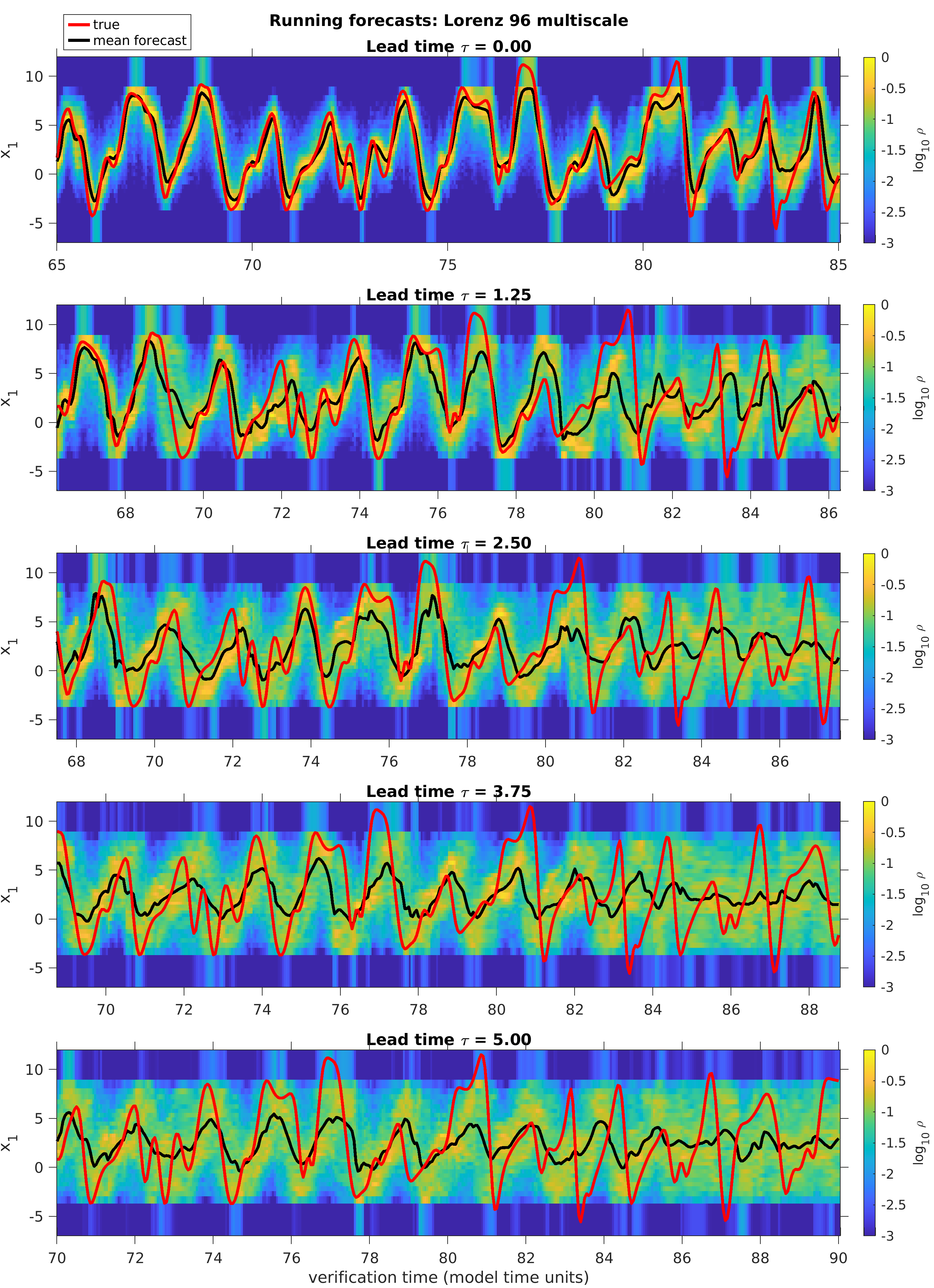
Figure 2: Running QMDA forecasts of the $\mathsf{x}_{1}$ variable of the L96 multiscale system in a chaotic regime. The panels show the true $\mathsf{x}_{1}$ evolution (black lines), the logarithm of the discrete forecast probability density $\varrho_{n,j}$ (colors), and the corresponding forecast mean (red lines) as a function of verification time for lead times in the range 0–5 model time units (top to bottom). The assimilated observable is the $K$-dimensional vector of the L96 slow variables, $h=(x_{1},\ldots,x_{K})$, of the L96 system.

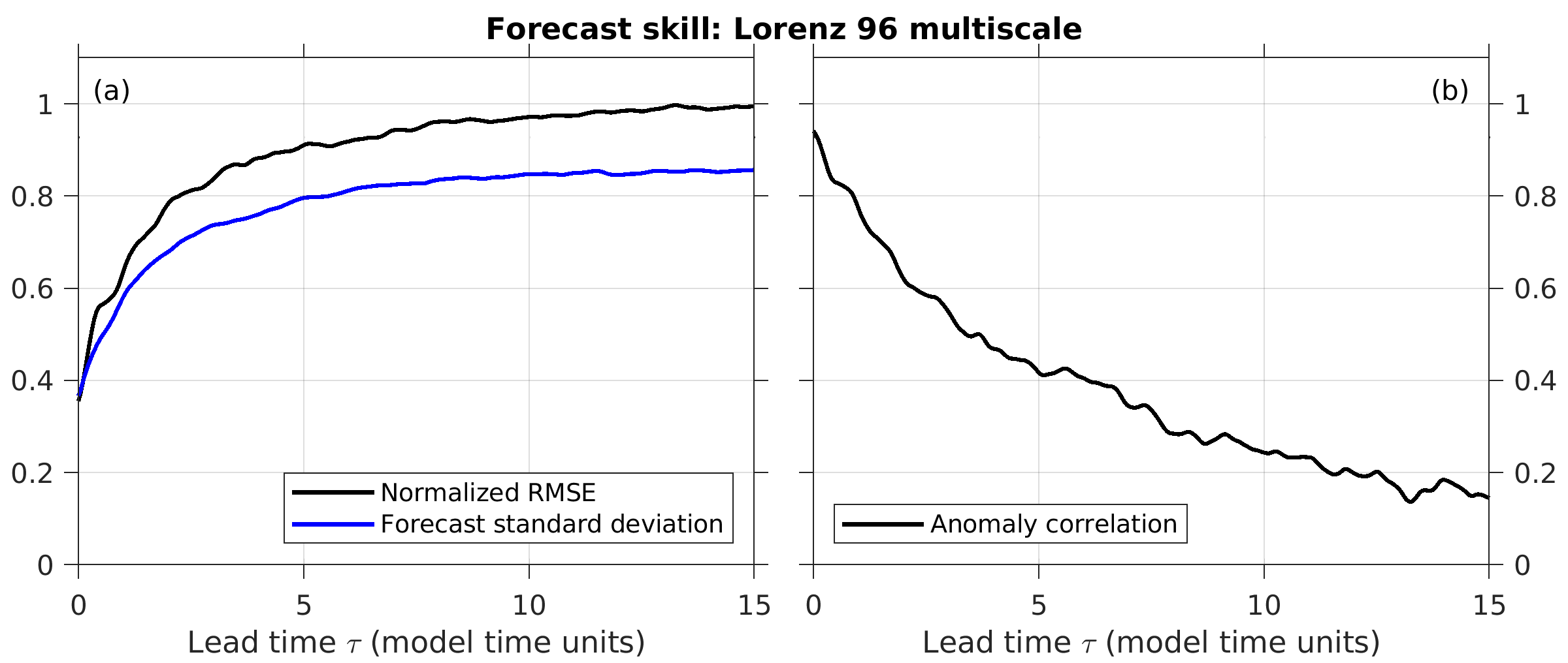
Figure 3: NRMSE (left) and AC score (right) of the L96 forecasts from Fig. 2.

Starting from $\omega_{0}$, QMDA produces a sequence of states $\omega_{0},\omega_{1},\ldots,\omega_{\hat{N}-1}$ by repeated application of the forecast–analysis steps, as depicted schematically in Fig. 1 and in pseudocode form in Algorithm 1. Specifically, for $n\in\{1,\ldots,\hat{N}-1\}$, we compute $\omega_{n}$ by first using the transfer operator to compute the state $\omega_{n-1,1}:=\mathcal{P}^{(\Delta t)}_{L,N}\omega_{n-1}$ (which is analogous to the prior in classical data assimilation), and then applying the effect map to observation $\hat{y}_{n}$ to yield $\omega_{n}=\omega_{n-1}\rvert_{{\mathcal{F}}_{L,N}(\hat{y}_{n})}$ (which is analogous to the classical posterior). For each $n\in\{0,\ldots,\hat{N}-1\}$, we also compute forecast states $\omega_{n,j}=\mathcal{P}^{(\tau_{j})}_{L,N}\omega_{n}$ and associated forecast distributions $\mathbb{P}_{n,j}$ for the observable $f$. We evaluate $\mathbb{P}_{n,j}$ on the bins $S_{m}$ and normalize the result by the corresponding bin size, $s_{m}:=\operatorname{length}(S_{M})$ to produce discrete probability densities $\varrho_{n,j}=(\varrho_{n,j,0},\ldots,\varrho_{n,j,M-1})$ with $\varrho_{n,j,m}:=\mathbb{P}_{n,n}(S_{m})/s_{m}$. We also compute the forecast mean and standard deviation, $\bar{f}_{n,j}=\omega_{\rho_{n,j}}A_{L,N}$ and $\sigma_{n,j}=(\omega_{\rho_{n,j}}(A_{L,N})^{2}-\bar{f}_{n,j}^{2})^{1/2}$, respectively. We assess forecast skill through the normalized mean square error (NRMSE) and anomaly correlation (AC) scores, computed for each lead time $\tau_{j}$ by averaging over the $\hat{N}$ samples in the verification dataset; see Appendix C.

Figure 2 shows the forecast probability densities $\varrho_{n,j}$ (colors), forecast means $\bar{f}_{n,j}$ (black lines), and true signal $\hat{f}_{n+j}$ (red lines), plotted as a function of verification time $t_{n+j}$ over intervals spanning 20 time units for representative lead times $\tau_{j}$ in the range 0 to 5 time units. The corresponding NRMSE and AC scores are displayed in Fig. 3. Given the turbulent nature of the dynamics, we intuitively expect the forecast densities $\varrho_{n,j}$ to start from being highly concentrated around the true signal for small $\tau_{j}$, and progressively broaden as $\tau_{j}$ increases (i.e., going down the panels of Fig. 2), indicating that the forecast uncertainty increases. Correspondingly, we expect the mean $\bar{f}_{n,j}$ to accurately track the true signal for $\tau_{j}$, and progressively relax towards the equilibrium mean $\int_{X}f\,d\mu$.

The results in Figs. 2 and 3 are broadly consistent with this behavior: The forecast starts at $\tau_{j}=0$ from a highly concentrated density around the true signal (note that Fig. 2 shows logarithms of $\varrho_{n,j}$), which is manifested by low NRSME and large AC values in Fig. 3 of approximately 0.35 and 0.95, respectively. As $\tau_{j}$ increases, the forecast distribution broadens, and the NRMSE (AC) scores exhibit a near-monotonic increase (decrease). In Fig. 3(a), the estimated error based on the forecast variance $\sigma_{n,j}$ is seen to track well the NRMSE score, which indicates that the forecast distribution $\varrho_{n,j}$ provides an adequate representation of forecast uncertainty. It should be noted that errors are present even at time $\tau_{j}=0$, particularly for periods of time where the true signal takes extreme positive or negative values. Such reconstruction errors are expected for a fully data-driven driven method applied to a system with a high-dimensional attractor. Overall, the skill scores in Fig. 3 are comparable with the results obtained in ref. [6] using kernel analog forecasting (KAF).

4 El Niño Southern Oscillation

The El Niño Southern Oscillation (ENSO) [5] is the dominant mode of interannual (3–5 year) variability of the Earth’s climate system. Its primary manifestation is an oscillation between positive sea surface temperature (SST) anomalies over the eastern tropical Pacific Ocean, known as El Niño events, and episodes of negative anomalies known as La Niña events [50]. Through atmospheric teleconnections, ENSO drives seasonal weather patterns throughout the globe, affecting the occurrence of extremes such as floods and droughts, among other natural and societal impacts [40]. Here, we demonstrate that QMDA successfully predicts ENSO within a comprehensive climate model by assimilating high-dimensional SST data.

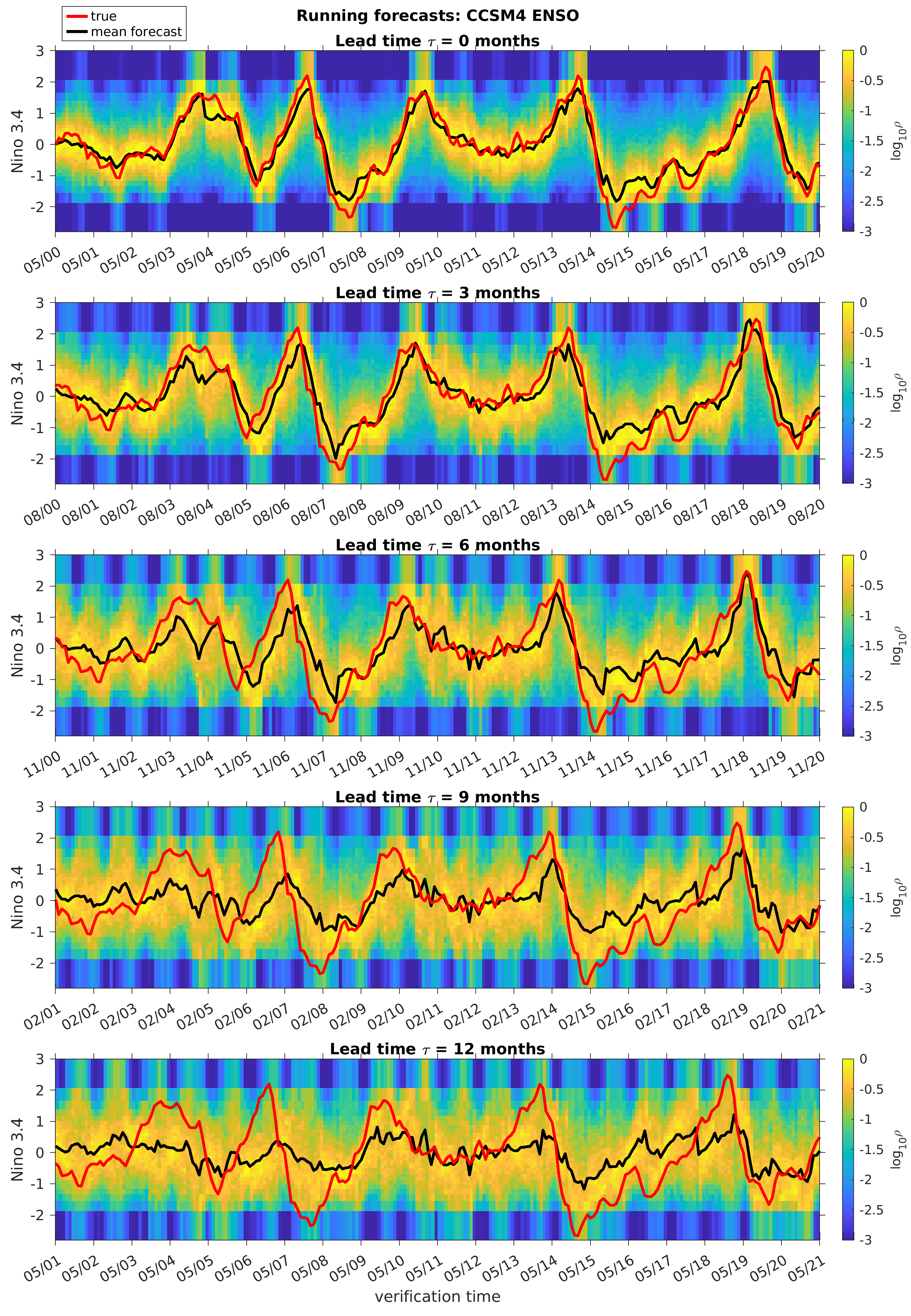
Figure 4: As in Fig. 2, but for forecasts of the Niño 3.4 index in CCSM4. The assimilated observable is the vector of Indo-Pacific SST gridpoint values. The forecast lead times are in 3-month increments in the range 0–12 months. The verification times ($x$-axes) are shown in mm/yy date format relative to an arbitrary year in the verification interval.

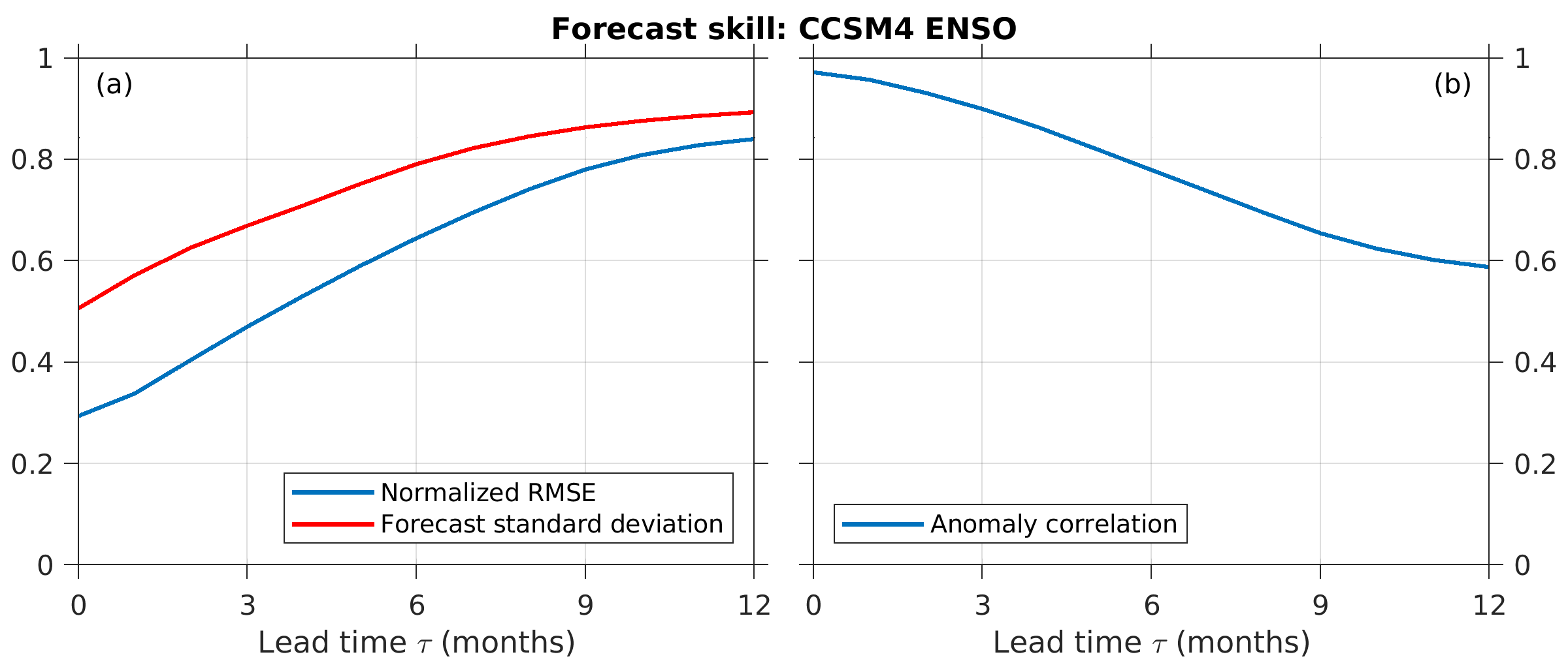
Figure 5: NRMSE (a) and AC score (b) of the Niño 3.4 forecasts from Fig. 4.

Our experimental setup follows closely ref. [51], who performed data-driven ENSO forecasts using KAF. As training and test data, we use a control integration of the Community Climate System Model Version 4 (CCSM4) [19], conducted with fixed pre-industrial greenhouse gas forcings. The simulation spans 1300 years, sampled at an interval $\Delta t=1$ month. Abstractly, the dynamical state space $X$ consists of all degrees of freedom of CCSM4, which is of order $10^{7}$ and includes variables such as density, velocity, and temperature for the atmosphere, ocean, and sea ice, sampled on discretization meshes over the globe. Since this simulation has no climate change, there is an implicit invariant measure $\mu$ sampled by the data, and we can formally define the algebras $\mathfrak{A}$ and $\mathfrak{B}$ associated with the invariant measure as described above.

In our experiments, the observation map $h:X\to Y$ returns monthly-averaged SST fields on an Indo-Pacific domain; that is, we have $Y=\mathbb{R}^{d}$ where $d$ is the number of surface ocean gridpoints within the domain. We have $d=\text{44,414}$, so these experiments test the ability of QMDA to assimilate high-dimensional data. However, note that $h$ is a highly non-invertible map since Indo-Pacific SST comprises only a small subset of CCSM4’s dynamical degrees of freedom. As our forecast observable $f\in\mathfrak{A}$ we choose the Niño 3.4 index—a commonly used index for ENSO monitoring defined as the average SST anomaly over a domain in the tropical Pacific Ocean. Large positive (negative) values of Niño 3.4 represent El Niño (La Niña) conditions, whereas values near zero represent neutral conditions. Additional information on the CCSM4 data is included in Section D.2.

Following ref. [51], we use the SST and Niño 3.4 samples from the first 1,100 years of the simulation as training data, and the corresponding samples for the last 200 years as test data. Thus, with the notation of the previously described L96 experiments, our training data are $y_{n}=h(x_{n})$ (Indo-Pacific SST) and $f_{n}=f(x_{n})$ (Niño 3.4) for $n\in\{0,\ldots,N-1\}$ and $N=\text{1,100}\times 12=13,200$, and our test data are $\hat{y}_{n}=h(x_{n+N})$ and $\hat{f}_{n}=f(x_{n+N})$ for $n\in\{0,\ldots,\hat{N}-1\}$ and $\hat{N}=200\times 12=2400$. Here, $x_{n}=\Phi^{n\,\Delta t}(x_{0})\in X$ is the (unknown) dynamical trajectory of the CCSM4 model underlying our training and test data. Using the SST samples $y_{n}$, we build the training data $z_{n}$ using delay-coordinate maps with parameter $Q=5$; i.e., the data $z_{n}$ used for building the data-driven basis of $H_{L,N}$ consist of SST “videos” that span a total of $2Q+1=11$ months. We use $L=3000$ dimensions. Following computation of the basis vectors $\phi_{l,N}$, the procedure for initializing and running QMDA is identical to our L96 experiments, and we will use the same notation to present results for ENSO.

Figure 4 shows the forecast probability density ($\varrho_{n,j}$; colors), forecast mean ($\bar{f}_{n,j}$; black lines), and true signal ($\hat{f}_{n+j}$; red lines) as a function of verification time $t_{n+j}$ over 20-year portions of the test dataset for lead times $\tau_{j}$ in the range 0 to 12 months. The corresponding NRMSE and AC scores are displayed in Fig. 5. Qualitatively, the forecast density $\varrho_{n,j}$ displays a similar behavior as in the L96 experiments; that is, it is concentrated around the true signal on short lead times ($\tau_{j}\lesssim 3$ months), and gradually broadens as forecast uncertainty grows with increasing lead time $\tau_{j}$ due to chaotic climate dynamics. In Fig. 5(a), the estimated forecast error based on the forecast variance $\sigma_{n,j}$ agrees reasonably well with the actual NRMSE evolution. Adopting $\text{AC}=0.6$ as a commonly used threshold for ENSO predictability, we see from the AC results in Fig. 5(b) that QMDA produces useful forecasts out to $\tau_{j}\simeq 12$ months. The performance of QMDA in terms of the NRMSE and AC metrics is comparable to that found for KAF in ref. [51], but QMDA has the advantage of producing full forecast probability distributions instead of point estimates. Compared to KAF, QMDA also has the advantage of being positivity-preserving. While failure to preserve signs may not be critical for sign-indefinite ENSO indices, there are many climatic variables such as temperature or moisture where sign preservation is particularly important.

5 Concluding remarks

We have developed new theory and methods for sequential data assimilation of partially observed dynamical systems using techniques from operator algebra, quantum information, and ergodic theory. At the core of this framework, called quantum mechanical data assimilation (QMDA), is the non-abelian algebraic structure of spaces of operators. One of the main advantages that this structure provides is that it naturally enables finite-dimensional discretization schemes that preserve the sign of sign-definite observables in ways that are not possible with classical projection-based approaches.

We build these schemes starting from a generalization of Bayesian data assimilation based on a dynamically consistent embedding into an infinite-dimensional operator algebra, to our knowledge described here for the first time. Under this embedding, forecasting is represented by a quantum operation induced by the Koopman operator of the dynamical system, and Bayesian analysis is represented by quantum effects. In addition to providing a useful starting point for discretizing data assimilation, this construction draws connections between statistical inference methods for classical dynamical systems with quantum information and quantum probability, which should be of independent interest.

QMDA leverages properties of operator algebras to project the infinite-dimensional framework into the level of a matrix algebra in a manner that positive operators are represented by positive matrices, and the finite-dimensional system is a quantum operation. QMDA also has a data-driven formulation based on kernel methods for machine learning with consistent asymptotic behavior as the amount of training data increases. We have demonstrated the efficacy of QMDA with forecasting experiments of the slow variables of the Lorenz 96 multiscale system in a chaotic regime and the El Niño Southern Oscillation in a climate model. QMDA was shown to perform well in terms of point forecasts from quantum mechanical expectations, while also providing uncertainty quantification by representing entire forecast distributions via quantum states.

This work motivates further application and development of algebraic approaches and quantum information to building models and performing inference of complex dynamical systems. In particular, as we enter the quantum computing era, there is a clear need to lay out the methodological and algorithmic foundations for quantum simulation of complex classical systems. Being firmly rooted in quantum information and operator theory, the QMDA framework presented in this paper is a natural candidate for implementation in quantum computers. As noted in the opening section of the paper, efforts to simulate classical dynamical systems on quantum computers are being actively pursued [29, 37, 23]. Porting data assimilation algorithms such as QMDA to a quantum computational environment presents new challenges as the iterative nature of the forecast–analysis cycle will require repeated interaction between the quantum computer and the assimilated classical system. We believe that addressing these challenges is a fruitful area for future research with both theoretical and applied dimensions.

Appendix A Assumptions

We make the following standing assumption on the dynamical system and forecast observable.

1. $\Phi^{t}:X\to X$, $t\in\mathbb{R}$, is a continuous-time, continuous flow, on a compact metrizable space $X$.

2. $\mu$ is an invariant, ergodic, Borel probability measure under $\Phi^{t}$.

3. The forecast observable $f:X\to\mathbb{R}$ is a real-valued function lying in $\mathfrak{A}=L^{\infty}(X,\mu)$.

Note that the support of $\mu$ is a closed subset of the compact space $X$, and thus is compact. Moreover, the compactness assumption on $X$ can be replaced by the weaker assumption that $\Phi^{t}$ has a forward-invariant compact set $X_{+}$ that contains the support of $\mu$ (which is again necessarily compact). The analysis performed below can be carried over to this setting by replacing the space of continuous functions $C(X)$ (which is a Banach space equipped with the uniform norm when $X$ is compact) with $C(X_{+})$.

For the purpose of data-driven approximation, we additionally require:

1. For the sampling interval $\Delta t>0$, the discrete-time system induced by the map $\Phi^{\Delta t}:X\to X$ is ergodic with respect to $\mu$.

2. The forecast observable $f:X\to\mathbb{R}$ is continuous.

3. The observation map $h:X\to Y$ is continuous.

Appendix A(a) implies that for $\mu$-a.e. initial condition $x_{0}\in X$, the sampling measures $\mu_{N}=\sum_{n=0}^{N-1}\delta_{x_{n}}/N$ with $x_{n}=\Phi^{n\,\Delta t}(x_{0})$ weak-^∗ converge to the invariant measure $\mu$; that is,

(15) $$\lim_{N\to\infty}\int_{X}f\,d\mu_{N}=\lim_{N\to\infty}\frac{1}{N}\sum_{n=0}^{N-1}f(x_{n})=\int_{X}f\,d\mu,\quad\forall f\in C(X).$$

Henceforth, we will assume for convenience that the states $x_{0},x_{1},\ldots$ are all distinct—aside from the trivial case that the support of $\mu$ is a singleton set consisting of a fixed point, this assumption holds for $\mu$-a.e. initial condition $x_{0}$, and ensures that the Hilbert space $\hat{H}_{N}=L^{2}(X,\mu_{N})$ has dimension $N$.

In what follows,

$$\langle f,g\rangle=\int_{X}f^{*}g\,d\mu,\quad\langle f,g\rangle_{N}=\int_{X}f^{*}g\,d\mu_{N}=\frac{1}{N}\sum_{n=0}^{N-1}f^{*}(x_{n})g(x_{n})$$

will denote the inner products of $H$ and $\hat{H}_{N}$, respectively. The Hilbert space $\hat{H}_{N}$ is isomorphic to $\mathbb{C}^{N}$ equipped with the normalized dot product $\bm{f}\cdot\bm{g}\equiv\bm{f}^{\dagger}\bm{g}/N$, where $\bm{f}^{\dagger}$ is the Hermitian conjugate (complex conjugate transpose) of the column vector $\bm{f}\in\mathbb{C}^{N}$. Under this isomorphism, two elements $f,g\in\hat{H}_{N}$ are represented by column vectors $\bm{f}=(f(x_{0}),\ldots,f(x_{N-1}))^{\top}$ and $\bm{g}=(g(x_{0}),\ldots,g(x_{N-1}))^{\top}$, and we have $\langle f,g\rangle_{N}=\bm{f}\cdot\bm{g}$.

Appendix B Finite-dimensional approximation

This section provides an overview and pseudocode listings of the data-driven approximation techniques underpinning QMDA. We begin with Algorithm 1, which gives a high-level description of the QMDA pipeline employed in the L96 multiscale and CCSM4 experiments presented in the main text. The algorithm is divided up into two parts:

1. A training phase, which uses the training data $y_{0},\ldots,y_{N-1}\in Y$ and $f_{0},\ldots,f_{N-1}\in\mathbb{R}$ for the observation map $h$ and forecast observable $f$, respectively, to build an orthonormal basis $\{\phi_{0,N},\ldots,\phi_{L-1,N}\}$ of the Hilbert space $H_{L,N}$. The basis is used to approximate the Koopman operator $U^{t}$ of the dynamical system, the multiplication operator $\pi f$ representing the forecast observable, and the effect-valued map $\mathcal{F}$ employed in the analysis step.

2. A prediction phase, which iteratively executes the sequential forecast–analysis steps of QMDA given a test dataset of observations $\hat{y}_{0},\ldots,\hat{y}_{\hat{N}-1}\in Y$. The state of the data assimilation system at time $t_{n}$ is a vector state of the operator algebra $\mathfrak{B}_{L,N}$, induced by a unit vector $\xi_{n}\in H_{L,N}$. This vector is represented in the $\{\phi_{l,N}\}$ basis of $H_{L,N}$ by a column vector $\bm{\xi}_{n}\in\mathbb{C}^{L}$.

Algorithm 1 depends on a number of lower-level procedures, which we describe in the following subsections.

Algorithm 1 QMDA pipeline employed in the L96 and CCSM4 experiments described in the main text.

Inputs

1. Delay embedding parameter $Q\in\mathbb{N}$.

2. Hilbert space dimension $L\in\mathbb{N}$.

3. Number of spectral bins $M\in\mathbb{N}$.

4. Kernel neighborhood parameter $k_{\text{nn}}$ in $\mathbb{N}$.

5. Bandwidth exponent parameter $a>0$ and range parameters $J_{1},J_{2}\in\mathbb{N}$.

6. Number of forecast timesteps $J_{\text{f}}\in\mathbb{N}$.

7. Training data from observation map, $y_{-Q},\ldots,y_{N-1+Q}\in Y\equiv\mathbb{R}^{d}$ with $y_{n}=h(x_{n})$.

8. Training data from forecast observable, $f_{0},\ldots,f_{N-1+Q}\in\mathbb{R}$ with $f_{n}=f(x_{n})$.

9. Observed data $\hat{y}_{0},\ldots,\hat{y}_{\hat{N}-1}\in Y$ in test period.

Require: All training data are induced by the same sequence of (unknown) time-ordered states $x_{-Q},\ldots,x_{N-1+Q}\in X$ with $x_{n}=\Phi^{n\,\Delta t}(x_{0})$, taken at a fixed sampling interval $\Delta t>0$.

Outputs

1. Mean forecast $\{\bar{f}_{nj}\}$ for $n\in\{0,\ldots,\hat{N}-1\}$ and $j\in\{0,\ldots,J_{\text{f}}\}$, where $\bar{f}_{nj}$ has initialization time $t_{n}=n\,\Delta t$ in the test period and lead time $\tau_{j}=j\,\Delta t$.

2. Forecast uncertainty $\{\sigma_{nj}\}$ for $n\in\{0,\ldots,\hat{N}-1\}$ and $j\in\{0,\ldots,J_{\text{f}}\}$, where $\sigma_{nj}$ has initialization time $t_{n}$ and lead time $\tau_{j}$.

3. Spectral bins (intervals) $S_{0},\ldots,S_{M-1}\subseteq\mathbb{R}$.

4. Forecast probability vectors $\{\bm{p}_{nj}\}$ for $n\in\{0,\ldots,\hat{N}-1\}$ and $j\in\{0,\ldots,J_{\text{f}}\}$, where $\bm{p}_{nj}=(p_{0nj},\ldots,p_{M-1,nj})$ is the probability that, for initialization time $t_{n}$ and lead time $\tau_{j}$, the forecast observable $f$ lies in $S_{m}$.

Training phase

1. Apply (13) to the training data $y_{n}$ to build the delay-embedded dataset $z_{0},\ldots,z_{N-1}\in Z\equiv\mathbb{R}^{(2Q+1)d}$.

2. Set $d_{Z}$ to the Euclidean distance on $Z$. Execute Algorithm 2 with inputs $\{z_{n}\}_{n=0}^{N-1}$, $d_{Z}$, and $k_{\text{nn}}$ to obtain a kernel bandwidth function $b_{Z}:Z\to\mathbb{R}_{+}$.

3. Execute Algorithm 3 with inputs $\{z_{n}\}_{n=0}^{N-1}$, $d_{Z}$, and $k_{\text{nn}}$ to obtain basis vectors $\bm{\phi}_{0},\ldots,\bm{\phi}_{L-1}\in\mathbb{R}^{N}$ for $H_{L,N}$.

4. Execute Algorithm 7 with inputs $\{f_{n}\}_{n=0}^{N-1}$ to obtain spectral bins $S_{0},\ldots,S_{M-1}\subset\mathbb{R}$.

5. Execute Algorithm 6 with inputs $\{f_{n}\}_{n=0}^{N-1}$, $\{\bm{\phi}_{l}\}_{l=0}^{L-1}$, and $\{S_{m}\}_{m=0}^{M-1}$ to obtain the projected multiplication operator $\bm{A}\in\mathbb{M}_{L}$ representing $f$ and spectral projectors $\bm{E}_{0},\ldots,\bm{E}_{M-1}\in\mathbb{M}_{L}$.

6. For each $j\in\{1,\ldots,J_{\text{f}}\}$, execute Algorithm 8 with inputs $j$ and $\{\bm{\phi}_{l}\}_{l=0}^{L-1}$ to obtain Koopman operator matrices $\bm{U}^{(1)},\ldots,\bm{U}^{(J_{\text{f}})}\in\mathbb{M}_{L}$.

7. Set $d_{Y}$ to the Euclidean distance on $Y$. Execute Algorithm 2 with inputs $\{y_{n}\}_{n=0}^{N-1}$, $d_{Y}$, and $k_{\text{nn}}$ to obtain a kernel bandwidth function $b_{Y}:Y\to\mathbb{R}_{+}$.

8. Define the scaled distance function $\tilde{d}_{Y}:Y\times Y\to\mathbb{R}_{+}$ with $\tilde{d}_{Y}(y,y^{\prime})=d_{Y}(y,y^{\prime})/\sqrt{b_{Y}(y)b_{Y}(y^{\prime})}$. Execute Algorithm 2 with inputs $\{y_{n}\}_{n=0}^{N-1}$, $a$, $J_{1},J_{2}$, $\tilde{d}_{Y}$, and $\eta_{\text{bump}}$ (where $\eta_{\text{bump}}$ is the bump function from (37)) to obtain an optimal bandwidth parameter $\epsilon_{*}$.

9. Define the kernel function $\psi:Y\times Y\to[0,1]$ with $\psi(y,y^{\prime})=\eta_{\text{bump}}(\tilde{d}_{Y}(y,y^{\prime})/\epsilon_{*})$. Execute Algorithm 11 with inputs $\psi$, $\{y_{n}\}_{n=0}^{N-1}$ and $\{\bm{\phi}_{l}\}_{l=0}^{L-1}$ to obtain the effect-valued feature map $\bm{F}:Y\to\mathbb{M}_{L}$.

Prediction phase

1. Set the initial state vector $\bm{\xi}_{0}=(1,0,\ldots,0)^{\top}\in\mathbb{C}^{L}$.

2. For each $n\in\{1,\ldots,\hat{N}-1\}$ execute the forecast–analysis cycle in Algorithm 10 with inputs $J_{\text{f}}$, $J_{\text{o}}=1$, $\{\bm{U}^{(j)}\}_{j=1}^{J_{\text{f}}}$, $\bm{A}$, $\{\bm{E}_{m}\}_{m=0}^{M-1}$, $\bm{F}$, $\bm{\xi}_{n-1}$, and $\hat{y}_{n}$.

   Return:

   • The mean forecasts $\bar{f}_{n-1,0},\ldots,\bar{f}_{n-1,J_{\text{f}}}$.

   • The forecast uncertainties $\sigma_{n-1,0},\ldots,\sigma_{n-1,J_{\text{f}}}$.

   • The forecast probability vectors $\bm{p}_{n-1,0},\ldots,\bm{p}_{n-1,J_{\text{f}}}$.

   • The posterior state vector $\bm{\xi}_{n}$ given the observation $y_{n}$.

B.1 Kernel eigenfunctions

Following refs. [3, 24, 20, 21, 13], we use eigenvectors of kernel integral operators to construct both the $L$-dimensional Hilbert spaces $H_{L}$ and their data-driven counterparts $H_{L,N}$. We make the following assumptions on the kernels used to define these operators.

1. $k:X\times X\to\mathbb{R}$ is a continuous, symmetric kernel.

2. $k_{0},k_{1},\ldots:X\times X\to\mathbb{R}$ is a family of continuous, symmetric kernels such that, as $N\to\infty$, $k_{N}$ converges uniformly to $k$.

As we describe below, the kernels $k_{N}$ are typically data-dependent kernels obtained by normalization of a fixed (data-independent) kernel on $X$.

Defining $K:H\to H$ as the integral operator

$$Kf=\int_{X}k(\cdot,x)f(x)\,d\mu(x),$$

we have that $K$ is a real, self-adjoint, Hilbert-Schmidt operator, and thus there exists a real, orthonormal basis $\{\phi_{0},\phi_{1},\ldots\}$ of $H=L^{2}(X,\mu)$ consisting of eigenvectors of $K$,

(16) $$K\phi_{l}=\lambda_{l}\phi_{l},\quad\lambda_{l}\in\mathbb{R},$$

where the eigenvalues $\lambda_{0},\lambda_{1},\ldots$ are ordered in order of decreasing absolute value and converge to 0 as $l\to\infty$. In the data-driven setting, we replace $H$ by the $N$-dimensional Hilbert space $\hat{H}_{N}$, and define the integral operator $K_{N}:\hat{H}_{N}\to\hat{H}_{N}$ as

$$K_{N}f=\int_{X}k_{N}(\cdot,x)f(x)\,d\mu_{N}(x)=\frac{1}{N}\sum_{n=0}^{N-1}k_{N}(\cdot,x_{n})f(x_{n}).$$

The operator $K_{N}$ has an associated real, orthonormal eigenbasis $\{\phi_{0,N},\ldots,\phi_{N-1,N}\}$ of $\hat{H}_{N}$, where

(17) $$K_{N}\phi_{l,N}=\lambda_{l,N}\phi_{l,N},\quad\lambda_{l,N}\in\mathbb{R},$$

and the eigenvalues $\lambda_{l,N}$ are ordered again in order of decreasing modulus.

An important property of the eigenvectors $\phi_{l}$ and $\phi_{l,N}$ corresponding to nonzero eigenvalues is that they have continuous representatives. Specifically, assuming that $\lambda_{l}$ and $\lambda_{l,N}$ are nonzero, we define $\varphi_{l},\varphi_{l,N}\in C(X)$ such that

$$\varphi_{l}(x)=\frac{1}{\lambda_{l}}\int_{X}k(x,x^{\prime})\phi_{l}(x^{\prime})\,d\mu(x^{\prime}),\quad\varphi_{l,N}(x)=\frac{1}{\lambda_{l,N}}\int_{X}k_{N}(x,x^{\prime})\phi_{l,N}(x^{\prime})\,d\mu_{N}(x^{\prime}).$$

It then follows from (16) and (17), respectively, that $\varphi_{l}=\phi_{l}$ $\mu$-a.e. and $\varphi_{l,N}=\phi_{l,N}$ $\mu_{N}$-a.e. Note that the latter relation simply means that $\varphi_{l,N}(x_{n})=\phi_{l,N}(x_{n})$ for every $n\in\{0,\ldots,N-1\}$.

The following theorem summarizes the spectral convergence of the operators $K_{N}$ to $K$ and the convergence of the associated basis functions. The results are based on techniques developed in ref. [48]. Additional details and proofs for the setting of ergodic dynamical systems and data-dependent kernels employed in this work can be found, e.g., in refs. [13, 22].

Theorem B.1.

Under Appendix A, Appendix A, and Section B.1, the following hold as $N\to\infty$ for $\mu$-a.e. initial condition $x_{0}\in X$.

1. For each nonzero eigenvalue $\lambda_{l}$ of $K$, the sequence of eigenvalues $\lambda_{l,N}$ of $K_{N}$ converges to $\lambda_{l}$, including multiplicities.

2. If $\phi_{l}\in H$ is an eigenvector of $K$ corresponding to $\lambda_{l}$ with continuous representative $\varphi_{l}\in C(X)$, there exists a sequence of eigenvectors $\phi_{l,N}$ of $K_{N}$ corresponding to eigenvalue $\lambda_{l,N}$, whose continuous representatives $\varphi_{l,N}\in C(X)$ converge uniformly to $\varphi_{l}$.

In numerical applications, we use the $\hat{H}_{N}\simeq\mathbb{C}^{N}$ isomorphism to represent the eigenvectors $\phi_{l,N}$ by $N$-dimensional column vectors $\bm{\phi}_{l,N}\in\mathbb{C}^{N}$ (which are real since the $\phi_{l,N}$ are real) with $\bm{\phi}_{l,N}=(\phi_{l,N}(x_{0}),\ldots,\phi_{l,N}(x_{N-1}))^{\top}$. The vectors $\bm{\phi}_{l,N}$ are solutions of the eigenvalue problem

$$\bm{K}_{N}\bm{\phi}_{l,N}=\lambda_{l,N}\bm{\phi}_{l,N}$$

for the $N\times N$ kernel matrix $\bm{K}_{N}=[K_{ij,N}]_{i,j=0}^{N-1}$ with $K_{ij,N}=k_{N}(x_{i},x_{j})/N$. We impose the orthonormality condition $\bm{\phi}_{l,N}\cdot\bm{\phi}_{m,N}=\delta_{l,m}$, which is equivalent to $\langle\phi_{l,N},\phi_{m,N}\rangle_{N}=\delta_{lm}$ on $\hat{H}_{N}$.

Henceforth, we will assume that for a given choice of basis vectors $\phi_{l}$ of $H$ and so long as $\lambda_{l}$ is nonzero, the data-driven basis vectors $\phi_{l,N}$ of $\hat{H}_{N}$ are chosen such that they converge to $\phi_{l}$ as per Theorem B.1. This assumption leads to no loss of generality since every real, orthonormal eigenbasis $\phi_{l,N}$ can be orthogonally rotated to a basis that converges to $\phi_{l}$ without affecting the results of the computations presented below.

B.2 Choice of kernel

Since our training data $z_{n}$ are in the space $Z$, we employ kernels which are pullbacks of kernels on that space; specifically, we set $k(x,x^{\prime})=\kappa(z(x),z(x^{\prime}))$ and $k_{N}(x,x^{\prime})=\kappa_{N}(z(x),z(x^{\prime}))$, where $\kappa:Z\times Z\to\mathbb{R}$ and $\kappa_{N}:Z\times Z\to\mathbb{R}$ are continuous, symmetric kernels. With this approach, all kernel computations can be executed using the data $z_{n}\in Z$ without knowledge of the underlying dynamical states $x_{n}\in X$.

Following ref. [13], we construct the kernels $\kappa_{N}$ by applying the bistochastic normalization procedure introduced in ref. [9] to the family of variable-bandwidth diffusion kernels developed in ref. [4]. Using the training data $z_{n}$, we construct a variable-bandwidth radial basis function kernel $\tilde{\kappa}_{N}:Z\times Z\to\mathbb{R}$ of the form

(18) $$\tilde{\kappa}_{N}(z,z^{\prime})=\eta_{\text{gauss}}\left(\frac{d(z,z^{\prime})}{\epsilon_{N}\sqrt{b_{N}(z)b_{N}(z^{\prime})}}\right),$$

where $\eta_{\text{gauss}}:\mathbb{R}\to\mathbb{R}$ is the Gaussian shape function, $\eta_{\text{gauss}}(u)=e^{-u^{2}}$, $d:Z\to Z\to\mathbb{R}_{+}$ is a distance function (which we nominally set to the Euclidean when $Z=\mathbb{R}^{d}$), $\epsilon_{N}>0$ is a bandwidth parameter, and $b_{N}:Z\to\mathbb{R}_{+}$ is a (data-dependent) bandwidth function. The construction of the bandwidth function, which resembles a kernel density estimation procedure, is summarized in Algorithm 2. The bandwidth parameter $\epsilon_{N}$ is tuned automatically via Algorithm 5, which is described in Section B.3 below. Further details on Algorithms 2 and 5 can be found in refs. [3, 4].

Algorithm 2 Kernel bandwidth function.

Inputs

1. Dataset $x_{0},x_{1},\ldots,x_{N-1}\in\mathcal{X}$; $\mathcal{X}$ is an arbitrary set.

2. Distance function $d:\mathcal{X}\times\mathcal{X}\to\mathbb{R}_{+}$.

3. Neighborhood parameter $k_{\text{nn}}\in\mathbb{N}$.

4. Bandwidth exponent parameter $a>0$ and range parameters $J_{1},J_{2}\in\mathbb{N}$.

Outputs

1. Bandwidth function $b:\mathcal{X}\to\mathbb{R}_{+}$.

Steps

1. Construct the function $r:\mathcal{X}\to\mathbb{R}_{+}$, where $r^{2}(x)=\sum_{j=1}^{k_{\text{nn}}}d^{2}(x,I(x,j))/k_{\text{nn}}$ and $I(x,j)\in\{0,\ldots,N-1\}$ is the index of the $j$-th nearest neighbor of $x$ in the $\{x_{i}\}_{i=0}^{N-1}$ dataset with respect to the distance $d$.

2. Construct the distance-like function $\tilde{d}:\mathcal{X}\times\mathcal{X}\to\mathbb{R}$ with $\tilde{d}(x,x^{\prime})=d(x,x^{\prime})/\sqrt{r(x)r(x^{\prime})}$.

3. Execute Algorithm 5 with inputs $\{x_{n}\}_{n=0}^{N-1}$, $\tilde{d}$, $\eta_{\text{gauss}}$, $k_{\text{nn}}$, $a$, $J_{1}$, and $J_{2}$ to obtain an optimal bandwidth $\epsilon_{*}$ and dimension estimate $m_{*}$.

4. Construct the kernel $\tilde{k}:\mathcal{X}\times\mathcal{X}\to\mathbb{R}_{+}$, where $\tilde{k}(x,x^{\prime})=\eta_{\text{gauss}}(\tilde{d}(x,x^{\prime})/\epsilon_{*})$.

5. Return: The function $b:\mathcal{X}\to\mathbb{R}_{+}$ such that $b(x)=\sum_{j=0}^{N-1}\tilde{k}(x,x_{j})/(N(\pi\epsilon_{*}r^{2}(x))^{m_{*}/2})$.

Using the kernel $\tilde{\kappa}_{N}$, we perform the sequence of normalization steps described in ref. [9] to obtain a symmetric, positive, positive-definite kernel $\kappa_{N}$ which is Markovian with respect to the pushforward $\nu_{N}:=z_{*}(\mu_{N})$ of the sampling measure on $Z$,

$$\int_{Z}\kappa_{N}(z,z^{\prime})\,d\nu_{N}(z^{\prime})=\frac{1}{N}\sum_{n=0}^{N-1}\kappa_{N}(z,z_{n})=1,\quad\forall z\in Z.$$

Algorithm 3 describes the computation of the eigenvectors $\bm{\phi}_{l,N}$ associated with this kernel. We note that due to the particular form of the normalization leading to $\kappa_{N}$, the eigenvectors $\bm{\phi}_{l,N}$ can be computed without explicit formation of the $N\times N$ kernel matrix $\bm{K}_{N}$. Instead, we compute the $\bm{\phi}_{l,N}$ through the singular value decomposition (SVD) of an $N\times N$ kernel matrix $\tilde{\bm{K}}_{N}=[\tilde{\kappa}_{N}(z_{i},z_{j})]_{i,j=0}^{N-1}$ associated with a non-symmetric kernel function $\tilde{\kappa}_{N}:Z\times Z\to\mathbb{R}$ that factorizes $\bm{K}_{N}$ as $\bm{K}_{N}=N\tilde{\bm{K}}_{N}\tilde{\bm{K}}_{N}^{\top}$. The steps leading to $\tilde{\kappa}_{N}$ are listed in Algorithm 4. See Appendix B in ref. [13] for further details.

Algorithm 3 Orthonormal basis vectors of $\hat{H}_{N}$ from variable-bandwidth bistochastic kernel. We suppress $N$ subscripts from our notation for $\bm{\phi}_{l,N}$.

Inputs

1. Dataset $z_{0},z_{1},\ldots,z_{N-1}\in Z$.

2. Distance function $d:Z\times Z\to\mathbb{R}_{+}$.

3. Neighborhood parameter $k_{\text{nn}}\in\mathbb{N}$.

4. Bandwidth exponent parameter $a>0$ and range parameters $J_{1},J_{2}\in\mathbb{N}$.

5. Number of basis vectors $L\leq N$.

Outputs

1. Column vectors $\bm{\phi}_{0},\ldots,\bm{\phi}_{L-1}\in\mathbb{R}^{N}$.

Steps

1. Execute Algorithm 2 with inputs $\{z_{n}\}_{n=0}^{N-1}$, $d$, $a$, $J_{1}$, and $J_{2}$ to obtain a bandwidth function $r:Z\to\mathbb{R}_{+}$.

2. Construct the distance-like function $\tilde{d}:Z\times Z\to\mathbb{R}_{+}$ with $\tilde{d}(z,z^{\prime})=d(z,z^{\prime})/\sqrt{r(z)r(z^{\prime})}$.

3. Execute Algorithm 5 with inputs $\{z_{n}\}_{n=0}^{N-1}$, $\tilde{d}$, $\eta_{\text{gauss}}$, $a$, $J_{1}$, and $J_{2}$ to obtain an optimal bandwidth $\epsilon_{*}$ and dimension estimate $m_{*}$.

4. Construct the kernel $k:Z\times Z\to\mathbb{R}_{+}$ with $k(z,z^{\prime})=\eta_{\text{gauss}}(\tilde{d}(z,z^{\prime})/\epsilon_{*})$.

5. Execute Algorithm 4 with inputs $\{z_{n}\}_{n=0}^{N-1}$ and $k$ to obtain a non-symmetric kernel function $\hat{k}:Z\times Z\to\mathbb{R}_{+}$.

6. Form the $N\times N$ kernel matrix $\hat{\bm{K}}=[\hat{K}_{ij}]_{i,j=0}^{N-1}$ with $\hat{K}_{ij}=\hat{k}(z_{i},z_{j})$.

7. Return: The leading $L$ left singular vectors $\bm{\phi}_{0},\ldots,\bm{\phi}_{L-1}$ of $\hat{\bm{K}}$, arranged in order of decreasing corresponding singular value, and normalized such that $\lVert\bm{\phi}_{l}\rVert_{2}=\sqrt{N}$.

Algorithm 4 Factorization of bistochastic kernel function.

Inputs

1. Dataset $x_{0},x_{1},\ldots,x_{N-1}\in\mathcal{X}$; $\mathcal{X}$ is an arbitrary set.

2. Kernel function $k:\mathcal{X}\times\mathcal{X}\to\mathbb{R}_{+}$.

Outputs

1. Non-symmetric kernel function $\hat{k}:\mathcal{X}\times\mathcal{X}\to\mathbb{R}$.

Steps

1. Construct the degree function $d:\mathcal{X}\to\mathbb{R}_{+}$, where $d(x)=\sum_{j=0}^{N-1}k(x,x_{j})$.

2. Construct the function $q:\mathcal{X}\to\mathbb{R}_{+}$, where $q(x)=\sum_{j=0}^{N-1}k(x,x_{j})/d(x_{j})$.

3. Return: The kernel function $\hat{k}:\mathcal{X}\times\mathcal{X}\to\mathbb{R}_{+}$, where $\hat{k}(x,x^{\prime})=k(x,x^{\prime})/(d(x)q^{1/2}(x^{\prime}))$.

In addition to the bistochastic kernel from Algorithm 3, QMDA can be implemented with a variety of kernels, including non-symmetric kernels satisfying a detailed-balance condition (e.g., the family of normalized kernels from the diffusion maps algorithm [10]). Two basic guidelines on kernel choice are that the data-dependent kernels $k_{N}$ are regular-enough such that the integral operators $K_{N}$ converge spectrally to $K$ (in the sense of Theorem B.1), and the limit kernel $k$ is “rich-enough” such that all eigenvalues $\lambda_{l}$ are strictly positive (i.e., $k$ is an $L^{2}(\mu)$ integrally strictly-positive kernel [43]). In that case, as $N$ and $l$ increase, the eigenvectors $\phi_{l,N}$ provide a consistent approximation of an orthonormal basis for the entire Hilbert space $H$. The bistochastic kernels $k_{N}$ from Algorithm 3 have this property if the map $z:X\to Z$ is injective. The latter, holds for sufficiently large delay parameter $Q$ from (13) under appropriate assumptions on delay-coordinate maps [42].

For certain classes of kernels $k$ constructed from shape functions with rapid decay (e.g., the Gaussian shape function $\eta_{\text{gauss}}$), the asymptotic behavior of the eigenfunctions in the limit of vanishing bandwidth parameter $\epsilon_{N}$ may be studied using the theory of heat kernels [25]. Under appropriate conditions (e.g., the support of the invariant measure $\mu$ is a differentiable manifold or a metric measure space), the eigenfunctions are extremizers of a Dirichlet energy induced by the kernel, which defines a notion of regularity of functions akin to a Sobolev norm. In such cases, for any given $L\in\mathbb{N}$, the set of orthonormal vectors $\{\phi_{0},\ldots,\phi_{L-1}\}$ (which we will use in Section B.4 to define the subspaces $H_{L}\subset H$ used in QMDA) is optimal in the sense of having maximal regularity with respect to the kernel-induced Dirichlet energy.

B.3 Bandwidth tuning

Algorithm 5 is a tuning procedure for bandwidth-dependent kernels $k:\mathcal{X}\times\mathcal{X}\to\mathbb{R}_{+}$ of the form $k(x,x^{\prime})=\kappa(d(x,x^{\prime})/\epsilon)$, where $\mathcal{X}$ is an arbitrary set, $d:\mathcal{X}\times\mathcal{X}\to\mathbb{R}_{+}$ is a distance-like function, $\kappa:\mathbb{R}_{+}\to\mathbb{R}_{+}$ a positive kernel shape function, and $\epsilon>0$ a kernel bandwidth parameter. The tuning approach in Algorithm 5 was proposed in ref. [11] using scaling arguments for heat-like kernels on manifolds, and was also used in refs. [3, 4, 21]. It takes as input a dataset in $\mathcal{X}$ and a logarithmic grid of candidate bandwidth values $\epsilon_{j}$, and returns an “optimal“ bandwidth $\epsilon_{*}$ from this candidate set that maximizes a kernel-induced dimension function $m(\epsilon_{j})$ for the dataset. If $k$ is a heat-like kernel on a Riemannian manifold, $m(\epsilon_{*})$ is an estimator of the manifold’s dimension, but $m(\epsilon_{*})$ also provides a notion of dimension for non-smooth sets.

Algorithm 5 Tuning of bandwidth-dependent kernels.

Inputs

1. Dataset $x_{0},x_{1},\ldots,x_{N-1}\in\mathcal{X}$; $\mathcal{X}$ is an arbitrary set.

2. Bandwidth exponent parameter $a>0$ and range parameters $J_{1},J_{2}\in\mathbb{N}$.

3. Distance-like function $d:\mathcal{X}\times\mathcal{X}\to\mathbb{R}_{+}$.

4. Kernel shape function $\eta:\mathbb{R}_{+}\to\mathbb{R}_{+}$.

Outputs

1. Optimal bandwidth $\epsilon_{*}>0$.

2. Estimated dataset dimension $m_{*}\geq 0$.

Steps

1. Compute the $N\times N$ pairwise distance matrix $\bm{D}=[D_{ij}]_{i,j=0}^{N-1}$ with $D_{ij}=d(x_{i},x_{j})$.

2. Generate logarithmic grid $\{\epsilon_{j}\}_{j=J_{1}}^{J_{2}}$ with $\epsilon_{j}=2^{aj}$.

3. For each $j\in\{J_{1},\ldots,J_{2}\}$, compute the kernel sum $S(\epsilon_{j})=\sum_{i,l=0}^{N-1}K_{il}/N^{2}$, where $K_{il}=\eta(D_{il}/\epsilon_{j})$.

4. For each $j\in\{J_{1}+1,\ldots,J_{2}-1\}$, compute the logarithmic derivative

   $$m(\epsilon_{j})=\frac{\log S_{j+1}-\log S_{j-1}}{\log\epsilon_{j+1}-\log\epsilon_{j-1}}=\frac{\log(S_{j+1}/S_{j-1})}{2a}.$$

5. Return: $\epsilon_{*}=\operatorname*{argmax}_{\epsilon_{j}\in\{\epsilon_{J_{1}},\ldots,\epsilon_{J_{2}}\}}m(\epsilon_{j})$ and $m_{*}=m(\epsilon_{*})$.

B.4 Finite-dimensional Hilbert spaces and operator approximation

Given the basis vectors $\phi_{l}$ and $\phi_{l,N}$ from Section B.1, we define the $L$-dimensional Hilbert spaces

$$H_{L}=\operatorname{span}\{\phi_{0},\ldots,\phi_{L-1}\}\subset H,\quad H_{L,N}=\operatorname{span}\{\phi_{0,N},\ldots,\phi_{L-1,N}\}\subset\hat{H}_{N},$$

where in the case of $H_{L,N}$ $L$ is at most $N$. As in the main text, we let $\Pi_{L}:H\to H$ and $\Pi_{L,N}:\hat{H}_{N}\to\hat{H}_{N}$ be the orthogonal projections on $H$ and $\hat{H}_{N}$, respectively, with $\operatorname{ran}\Pi_{L}=H_{L}$ and $\operatorname{ran}\Pi_{L,N}=H_{L,N}$. We also let $\bm{\Pi}_{L}:\mathfrak{B}\to\mathfrak{B}$ and $\bm{\Pi}_{L,N}:\hat{\mathfrak{B}}_{N}\to\hat{\mathfrak{B}}_{N}$ be the induced projections on the operator algebras $\mathfrak{B}=B(H)$ and $\mathfrak{B}_{N}=B(\hat{H}_{N})$, defined as $\bm{\Pi}_{L}A=\Pi_{L}A\Pi_{L}$ and $\bm{\Pi}_{L,N}A=\Pi_{L,N}\hat{A}\Pi_{L,N}$, respectively. Defining $\mathfrak{B}_{L}=\operatorname{ran}\bm{\Pi}_{L}$, we can canonically identify $\mathfrak{B}_{L}$ with the subalgebra of $\mathfrak{B}$ consisting of all operators $A$ satisfying $\ker A\supseteq H_{L}$ and $\operatorname{ran}A\subseteq H_{L}$. The space $\mathfrak{B}_{L,N}:=\operatorname{ran}\bm{\Pi}_{L,N}$ can be canonically identified with a subalgebra of $\hat{\mathfrak{B}}_{N}$ in a similar manner. We will be making these identifications whenever convenient.

Within this setting, we are interested in the following two types of operator approximation, respectively described in Sections B.4.1 and B.4.2.

1. Approximation of an operator $A\in\mathfrak{B}$ by a finite-rank operator $A_{L}\in\mathfrak{B}_{L}$.

2. Approximation of $A_{L}\in\mathfrak{B}_{L}$ by an operator $A_{L,N}\in\mathfrak{B}_{L,N}$.

Intuitively, we think of an approximation of the first type listed above as a “compression” of an operator $A\in\mathfrak{B}$ of possibly infinite rank to an operator $A_{L}\in\mathfrak{B}_{L}\subset\mathfrak{B}$ of at most rank $L$. Approximations of the second type are of a fundamentally different nature since there are no inclusion relationships between $\mathfrak{B}_{L}$ and $\mathfrak{B}_{L,N}$. One can think instead of such approximations as data-driven approximations of the representation of an operator in a basis.

B.4.1 Operator compression

Given $A\in\mathfrak{B}$, we define $A_{L}\in\mathfrak{B}_{L}$ as

(19) $$A_{L}:=\bm{\Pi}_{L}A=\Pi_{L}A\Pi_{L},$$

Since $\{\phi_{0},\phi_{1},\ldots\}$ is an orthonormal basis of $H$, the projections $\Pi_{L}$ converge strongly to the identity; that is, for every $f\in H$, we have $\lim_{L\to\infty}(\Pi_{L}-I)f=0$, where the limit is taken in the norm of $H$. As a result, the operators $\breve{A}_{L}:=A\Pi_{L}$ converge strongly to $A$, $\lim_{L\to\infty}(\breve{A}_{L}-A)f=0$ for all $f\in H$. It then follows from standard results in functional analysis that $A_{L}=\Pi_{L}\breve{A}_{L}$ converges strongly to $A$, i.e,

(20) $$\lim_{L\to\infty}A_{L}f=Af,\quad\forall f\in H.$$

As we will see below, this type of strong operator convergence is sufficient to deduce convergence of the matrix mechanical formulation of data assimilation based on $\mathfrak{B}_{L}$ to the infinite-dimensional quantum mechanical level based on $\mathfrak{B}$ (see the rows labeled  and  in the schematic of Fig. 1).

B.4.2 Data-driven operator approximation

In order to facilitate approximation of operators in $\mathfrak{B}_{L}$ by operators in $\mathfrak{B}_{L,N}$, we use operators acting on the Banach space of continuous functions $C(X)$ as intermediate approximations. In what follows, we will let $\iota:C(X)\to H$ and $\iota_{N}:C(X)\to\hat{H}_{N}$ be the canonical linear maps that map continuous functions to their $L^{2}$ equivalence classes in $H$ and $\hat{H}_{N}$, respectively. In addition, we let $\mathfrak{C}=B(C(X))$ be the unital Banach algebra of bounded linear operators on $C(X)$. We assume $L\in\mathbb{N}$ is chosen such that the eigenvalues $\lambda_{L-1}$ and $\lambda_{L-1,N}$ of $K$ and $K_{N}$ from (16) and (17), respectively, are nonzero. This means that all elements of $H_{L}$ and $H_{L,N}$ have continuous representatives.

With these definitions and assumptions, we restrict attention to approximation of operators $A_{L}\in\mathfrak{B}_{L,N}$ which are obtained by applying (20) to operators $A\in\mathfrak{B}$ that satisfy

(21) $$A\circ\iota=\iota\circ\tilde{A},$$

for some $\tilde{A}\in\mathfrak{C}$. In addition, we assume that there is a uniformly bounded family of operators $\hat{A}_{N}\in\mathfrak{B}_{N}$ that satisfy an approximate version of (21) in the following sense: For every $f\in C(X)$, the norm of the residual $(\hat{A}_{N}\circ\iota_{N}-\iota_{N}\circ\tilde{A})f$ converges to 0. That is, we require

(22) $$\lim_{N\to\infty}\lVert R_{N}f\rVert_{\hat{H}_{N}}=0,\quad R_{N}=\hat{A}_{N}\circ\iota_{N}-\iota_{N}\circ\tilde{A},\quad\forall f\in C(X),$$

where the operators $\hat{A}_{N}$ satisfy the uniform norm bound

(23) $$\lVert\hat{A}_{N}\rVert_{\hat{\mathfrak{B}}_{N}}\leq a,$$

for a constant $a$. As we will see in the ensuing subsections, under Appendix A, all operators employed in QMDA satisfy (21), (22), and (23).

We have the following approximation lemma for the matrix elements of $A$ in terms of the matrix elements of $\hat{A}_{N}$.

Lemma B.2.

Suppose that $A\in\mathfrak{B}$, $\hat{A}_{N}\in\hat{\mathfrak{B}}_{N}$, and $\tilde{A}\in\mathfrak{C}$ satisfy (21), (22), and (23). Then, under Appendix A and Appendix A, and with the notation and assumptions of Section B.1, the matrix elements of $\hat{A}_{N}$ in the $\{\phi_{l,N}\}$ bases of $\hat{H}_{N}$ converge almost surely to the matrix elements of $A$ in the $\{\phi_{l}\}$ basis of $H$. That is, for $\mu$-a.e. initial condition $x_{0}\in X$, and every $i,j\in\mathbb{N}$ such that $\lambda_{i},\lambda_{j}\neq 0$,

$$\lim_{N\to\infty}\langle\phi_{i,N},\hat{A}_{N}\phi_{j,N}\rangle_{N}=\langle\phi_{i},A\phi_{j}\rangle.$$

Proof B.3.

See Section B.4.3.

Let $A_{ij}=\langle\phi_{i},A\phi_{j}\rangle$ and $A_{ij,N}=\langle\phi_{i,N},\hat{A}_{N}\phi_{j,N}\rangle_{N}$. The convergence of $A_{ij,N}$ to $A_{ij}$ from Lemma B.2 is not uniform with respect to $i,j\in\mathbb{N}$. However, restricting $i$ and $j$ to the finite index set $\{0,\ldots,L-1\}$ associated with the basis vectors of the finite-dimensional spaces $H_{L}$ and $H_{L,N}$ makes the convergence of $\hat{A}_{ij,N}$ to $\hat{A}_{ij}$ uniform, and we can conclude that the matrix representations of the projected operators $A_{L,N}=\bm{\Pi}_{L,N}\hat{A}_{N}$ converge to the matrix representation of $A_{L}=\bm{\Pi}_{L}A$.

Corollary B.4.

With notation as above, let $\bm{A}_{L}=[A_{ij}]_{i,j=0}^{L-1}$ and $\bm{A}_{L,N}=[A_{ij,N}]_{i,j=0}^{L-1}$ be the $L\times L$ matrix representations of $A_{L}$ and $A_{L,N}$ in the $\{\phi_{l}\}$ and $\{\phi_{l,N}\}$ bases of $H_{L}$ and $H_{L,N}$, respectively. Then, for $\mu$-a.e. initial condition $x_{0}$, we have $\lim_{N\to\infty}\bm{A}_{L,N}=\bm{A}_{L}$ in any matrix norm.

B.4.3 Proof of Lemma B.2

Recall from Section B.1 that the $\phi_{i,N}$ have continuous representatives $\varphi_{i,N}$ which converge $\mu$-a.s. to the continuous representatives $\varphi_{i}$ of $\phi_{i}$ in the uniform norm of $C(X)$. Note also that for every $N\in\mathbb{N}$, $\iota_{N}:C(X)\to\hat{H}_{N}$ has unit operator norm. Using these facts, we get

$$\lvert\langle\phi_{i,N},\hat{A}_{N}\phi_{j,N}\rangle_{N}-\langle\phi_{i},A\phi_{j}\rangle\rvert =\lvert\langle\phi_{i,N},\hat{A}_{N}\iota_{N}\varphi_{j,N}\rangle_{N}-\langle\phi_{i},A\phi_{j}\rangle\rvert$$

$$\leq\lvert\langle\phi_{i,N},\hat{A}_{N}\iota_{N}(\varphi_{j,N}-\varphi_{j})\rangle_{N}\rvert$$

$$\quad+\lvert\langle\phi_{i,N},\hat{A}_{N}\iota_{N}\varphi_{j}\rangle_{N}-\langle\phi_{i},A\phi_{j}\rangle\rvert$$

$$\leq a\lVert\varphi_{j,N}-\varphi_{j}\rVert_{C(X)}$$

(24) $$\quad+\lvert\langle\phi_{i,N},\hat{A}_{N}\iota_{N}\varphi_{j}\rangle_{N}-\langle\phi_{i},A\phi_{j}\rangle\rvert.$$

Moreover, we have

$$\lvert\langle\phi_{i,N},\hat{A}_{N}\iota_{N}\varphi_{j}\rangle_{N}-\langle\phi_{i},A\phi_{j}\rangle\rvert =\lvert\langle\phi_{i,N},\iota_{N}\tilde{A}\varphi_{j}\rangle_{N}+\langle\phi_{i,N}R_{N}\varphi_{j}\rangle_{N}-\langle\phi_{i},A\phi_{j}\rangle\rvert$$

$$\leq\lvert\langle\phi_{i,N},\iota_{N}\tilde{A}\varphi_{j}\rangle_{N}-\langle\phi_{i},A\phi_{j}\rangle\rvert+\lVert R_{N}\varphi_{j}\rVert_{\hat{H}_{N}}$$

$$=\lvert\langle\iota_{N}\varphi_{i,N},\iota_{N}\tilde{A}\varphi_{j}\rangle_{N}-\langle\phi_{i},A\phi_{j}\rangle\rvert+\lVert R_{N}\varphi_{j}\rVert_{\hat{H}_{N}}$$

$$=\lvert\langle\iota_{N}(\varphi_{i,N}-\varphi_{i}),\iota_{N}\tilde{A}\varphi_{j}\rangle_{N}+\langle\iota_{N}\varphi_{i},\iota_{N}\tilde{A}\varphi_{j}\rangle_{N}$$

$$\quad-\langle\phi_{i},A\phi_{j}\rangle\rvert+\lVert R_{N}\varphi_{j}\rVert_{\hat{H}_{N}}$$

$$\leq\lVert\varphi_{i,N}-\varphi_{i}\rVert_{C(X)}\lVert\tilde{A}\rVert_{\mathfrak{C}}\lVert\varphi_{j}\rVert_{C(X)}$$

(25) $$\quad+\lvert\langle\iota_{N}\varphi_{i},\iota_{N}\tilde{A}\varphi_{j}\rangle_{N}-\langle\phi_{i},A\phi_{j}\rangle\rvert+\lVert R_{N}\varphi_{j}\rVert_{\hat{H}_{N}}.$$

Now, by (21) we have

$$\lvert\langle\iota_{N}\varphi_{i},\iota_{N}\tilde{A}\varphi_{j}\rangle_{N}-\langle\phi_{i},A\phi_{j}\rangle\rvert =\lvert\langle\iota_{N}\varphi_{i},\iota_{N}\tilde{A}\varphi_{j}\rangle_{N}-\langle\iota\varphi_{i},A\iota\varphi_{j}\rangle\rvert$$

$$=\lvert\langle\iota_{N}\varphi_{i},\iota_{N}\tilde{A}\varphi_{j}\rangle_{N}-\langle\iota\varphi_{i},\iota\tilde{A}\varphi_{j}\rangle\rvert$$

$$=\left\lvert\int_{X}\varphi_{i}\tilde{A}\varphi_{j}d\mu_{N}-\int_{X}\varphi_{i}\tilde{A}\varphi_{j}\,d\mu\right\rvert,$$

so by the weak-^∗ convergence of $\mu_{N}$ to $\mu$ (see (15)) it follows that for $\mu$-a.e. initial condition $x_{0}$,

$$\lim_{N\to\infty}\lvert\langle\iota_{N}\varphi_{i},\iota_{N}\tilde{A}\varphi_{j}\rangle_{N}-\langle\phi_{i},A\phi_{j}\rangle\rvert=0.$$

Using this result, the uniform convergence of $\varphi_{i,N}$ to $\varphi_{i}$, and (22) in (25), we obtain

$$\lim_{N\to\infty}\lvert\langle\phi_{i,N},\hat{A}_{N}\iota_{N}\varphi_{j}\rangle_{N}-\langle\phi_{i},A\phi_{j}\rangle\rvert=0.$$

Finally, using the above and the uniform convergence of $\varphi_{i,N}$ to $\varphi_{i}$ in (24), we arrive at

$$\lim_{N\to\infty}\lvert\langle\phi_{i,N},\hat{A}_{N}\phi_{j,N}\rangle_{N}-\langle\phi_{i},A\phi_{j}\rangle\rvert=0,$$

which holds again for $\mu$-a.e. initial condition $x_{0}$. This completes the proof of the lemma.

B.5 Approximation of states

Let $\omega_{\rho}\in S_{*}(\mathfrak{B})$ be a normal state of $\mathfrak{B}$ induced by a density operator $\rho\in\mathfrak{B}_{*}$. We recall that the predual $\mathfrak{B}_{*}$ of $\mathfrak{B}$ is the space of trace-class operators on $H$ (denoted as $B_{1}(H)$ in the main text), equipped with the trace norm, $\lVert A\rVert_{\mathfrak{B}_{*}}=\operatorname{tr}\sqrt{A^{*}A}$. In the case of the finite-dimensional algebras $\mathfrak{B}_{L}$ and $\mathfrak{B}_{L,N}$, the preduals $\mathfrak{B}_{L*}$ and $\mathfrak{B}_{L,N*}$, respectively, can be identified with the algebras themselves, but we will continue to distinguish them using _∗ subscripts since they are equipped with a different norm (the trace norm) from the operator norm of the algebras.

As in Section B.4, we are interested in two types of state approximation, which can be thought of as state compression and data-driven approximation, respectively:

1. Approximation of $\rho$ by a finite-rank density operator $\rho_{L}\in\mathfrak{B}_{L}$; see Section B.5.1.

2. Approximation of $\rho_{L}$ by a data-driven density operator $\rho_{L,N}\in\mathfrak{B}_{L,N*}$; see Section B.5.2.

B.5.1 State compression

Similarly to Section B.4.1, for a given density operator $\rho\in\mathfrak{B}_{*}$ we define the projected operators $\sigma_{L}=\bm{\Pi}_{L}\rho$. Letting $C_{L}=\operatorname{tr}\sigma_{L}$, we have $C_{L}\leq\operatorname{tr}\rho=1$, so in general the $\sigma_{L}$ are not density operators. Nevertheless, the $\sigma_{L}$ are positive, finite-rank (and thus trace class) operators that converge to $\rho$ in trace norm (as opposed to merely strongly; cf. (20)). Indeed, we have $\rho-\sigma_{L}=(I-\Pi_{L})\rho(I-\Pi_{L})$, so $\rho-\sigma_{L}$ is positive, and

$$\|\rho-\sigma_{L}\rVert_{\mathfrak{B}_{*}}=\operatorname{tr}(\rho-\sigma_{L})=\sum_{l=L}^{\infty}\langle\phi_{l},\rho\phi_{l}\rangle,$$

where the sum in the right-hand side of the last equality is a positive, decreasing function of $L$, converging to 0 as $L\to\infty$. We also have $C_{L}=\sum_{l=0}^{L-1}\langle\phi_{l},\rho\phi_{l}\rangle$, which implies that $\lim_{L\to\infty}C_{L}=1$, and thus that there exists $L_{*}\in\mathbb{N}$ such that $C_{L}>0$ for all $L>L_{*}$. For any such $L$, $\rho_{L}:=\sigma_{L}/C_{L}$ is a density operator, and the sequence $\rho_{L}$ converges to $\rho$ in trace norm,

(26) $$\lim_{L\to\infty}\lVert\rho_{L}-\rho\rVert_{\mathfrak{B}_{*}}=0.$$

In the main text, we denote the map that sends the normal state $\omega_{\rho}\in S_{*}(\mathfrak{B})$ to $\omega_{\rho_{L}}\in S_{*}(\mathfrak{B}_{L})$ as $\bm{\Pi}^{\prime}_{L}(\rho)=\rho_{L}$.

Let now $A$ be an element of $\mathfrak{B}$ with corresponding projected elements $A_{L}=\bm{\Pi}_{L}A\in\mathfrak{B}_{L}$ from (19). By the cyclic property of the trace, we have $\operatorname{tr}(\rho_{L}A_{L})=\operatorname{tr}(\rho_{L}A)$, and the trace-norm convergence in (26) implies $\lim_{L\to\infty}\operatorname{tr}(\rho_{L}A_{L})=\operatorname{tr}(\rho A)$. Equivalently, letting $\omega_{\rho}\in S_{*}(\mathfrak{B})$ and $\omega_{\rho_{L}}$ be the states of $\mathfrak{B}$ and $\mathfrak{B}_{L}$ induced by $\rho$ and $\rho_{L}$, respectively, we have

(27) $$\lim_{L\to\infty}\omega_{\rho_{L}}A_{L}=\omega_{\rho}A.$$

We conclude that evaluation of the projected observables $A_{L}$ on the projected states $\omega_{\rho_{L}}$ asymptotically recovers the evaluation of $A$ on $\rho$.

B.5.2 Data-driven state approximation

Proceeding analogously to Section B.4.2, we seek data-driven approximations of projected density operators $\rho_{L}\in\mathfrak{B}_{L*}$ by density operators $\rho_{L,N}\in\mathfrak{B}_{L,N*}$ for a subset of density operators $\rho\in\mathfrak{B}_{*}$ that behave compatibly with bounded operators on continuous functions.

First, we recall that every density operator $\rho\in\mathfrak{B}_{*}$ admits a decomposition (diagonalization) of the form

(28) $$\rho=\sum_{j=0}^{\infty}r_{j}\langle\xi_{j},\cdot\rangle\xi_{j},$$

where $\{\xi_{0},\xi_{1},\ldots\}$ is an orthonormal basis of $H$, $(r_{0},r_{1},\ldots)$ is an $\ell^{1}$ sequence of real numbers in the interval $[0,1]$, and the sum over $j$ converges in the trace norm of $\mathfrak{B}_{*}$. In what follows, we shall restrict attention to a subset $S_{C}(\mathfrak{B})\subset S_{*}(\mathfrak{B})$, consisting of all normal states $\omega_{\rho}$ of $\mathfrak{B}$ whose corresponding density operators $\rho\in\mathfrak{B}_{*}$ are decomposable as in (28) with the following additional requirement: The orthonormal basis vectors $\xi_{j}$ have uniformly bounded continuous representatives; that is, we have

$$\xi_{j}=\iota\tilde{\xi}_{j},\quad\tilde{\xi}_{j}\in C(X),\quad\lVert\xi_{j}\rVert_{C(X)}\leq b,$$

for a constant $b$. Given such an $\omega_{\rho}\in S_{C}(\mathfrak{B})$, for each $N\in\mathbb{N}$ we define the positive operator $\hat{\sigma}_{N}:\hat{H}_{N}\to\hat{H}_{N}$, where

$$\hat{\sigma}_{N}=\sum_{j=0}^{\infty}r_{j}\langle\hat{\xi}_{j,N},\cdot\rangle_{N}\hat{\xi}_{j,N},\quad\hat{\xi}_{j,N}=\iota_{N}\tilde{\xi}_{j}.$$

Note that the well-definition of $\hat{\sigma}_{N}$ follows from the uniform boundedness of the $\tilde{\xi}_{j}$ and the fact that $(r_{0},r_{1},\ldots)$ is an $\ell^{1}$ sequence. It should also be kept in mind that, in general, the $\sigma_{N}$ are not normalized as density operators. We then have:

Lemma B.5.

1. $\tilde{\rho}:f\mapsto g$ with $g(x)=\sum_{j=0}^{\infty}r_{j}\langle\xi_{j},\iota f\rangle\tilde{\xi}_{j}(x)$ is well-defined as a linear map from $C(X)$ to itself, and it satisfies $\iota\circ\tilde{\rho}=\rho\circ\iota$.

2. For $\mu$-a.e. initial condition $x_{0}\in X$, the residual $R_{N}f=(\iota_{N}\circ\tilde{\rho})f-(\hat{\sigma}_{N}\circ\iota_{N})f$ satisfies

   $$\lim_{N\to\infty}\lVert R_{N}f\rVert_{\hat{H}_{N}}=0,\quad\forall f\in C(X).$$

Proof B.6.

See Section B.5.3.

It follows from Lemma B.5 that (21) and (22) hold with $A=\rho$, $\tilde{A}=\tilde{\rho}$, and $\hat{A}_{N}=\hat{\sigma}_{N}$. Thus, Lemma B.2 and Corollary B.4 apply, and for each $L\in\mathbb{N}$ such that $\lambda_{L-1}>0$, the matrix representations $\bm{\sigma}_{L,N}=[\langle\phi_{i,N},\hat{\sigma}_{N}\phi_{j,N}\rangle_{N}]_{i,j=0}^{L-1}$ of $\sigma_{L,N}=\Pi_{L,N}\hat{\sigma}_{N}$ converge to the matrix representation $\bm{\sigma}_{L}=[\langle\phi_{i},\rho\phi_{j}\rangle]_{i,j=0}^{L-1}$ of $\sigma_{L}=\bm{\Pi}_{L}\rho$. If, in addition, $L$ is sufficiently large such that $C_{L}>0$, then the density operators $\rho_{L,N}\in\mathfrak{B}_{L,N*}$ defined as $\rho_{L,N}=\sigma_{L,N}/C_{L,N}$ with $C_{L,N}=\operatorname{tr}\sigma_{L,N}$ converge, as $N\to\infty$, in the sense of convergence of the corresponding matrix representations $\bm{\rho}_{L,N}=\bm{\sigma}_{L,N}/C_{L,N}$, to the density operator $\rho_{L}=\sigma_{L}/C_{L}$ with matrix representation $\bm{\rho}_{L}=\bm{\sigma}_{L}/C_{L}$. As we saw in Section B.5.1, the latter converges to $\rho$ as $L\to\infty$ in the trace norm.

Combining the results of this section with those of Section B.4, we conclude that QMDA consistently approximates the action of normal states $\omega_{\rho}\in S_{C}(\mathfrak{B})$ on elements $A\in\mathfrak{B}$ satisfying (21) and (22) by the action of the data-driven states $\omega_{\rho_{L,N}}\in S(\mathfrak{B}_{L,N})$ on the data-driven elements $A_{L,N}\in\mathfrak{B}_{L,N}$ in the sense of the iterated limit

(29) $$\lim_{L\to\infty}\lim_{N\to\infty}\omega_{\rho_{L,N}}A_{L,N}=\lim_{L\to\infty}\omega_{\rho_{L}}A_{L}=\omega_{\rho}A,$$

where the first equality holds for $\mu$-a.e. initial condition $x_{0}\in X$.

B.5.3 Proof of Lemma B.5

(a)

Fix $x\in X$ and $\epsilon>0$. For any $x^{\prime}\in X$ and $J\in\mathbb{N}$, we have

$$\left\lvert\sum_{j=J}^{\infty}r_{j}\langle\xi_{j},f\rangle\left(\tilde{\xi}_{j}(x)-\tilde{\xi}_{j}(x^{\prime})\right)\right\rvert\leq\lVert f\rVert_{C(X)}\sum_{j=J}^{\infty}r_{j}\left\lvert\tilde{\xi}_{j}(x)-\tilde{\xi}_{j}(x^{\prime})\right\rvert\leq 2b\lVert f\rVert_{C(X)}\sum_{j=J}^{\infty}r_{j}.$$

Thus, since $(r_{0},r_{1},\ldots)\in\ell^{1}$, there exists $J$ such that $\left\lvert\sum_{j=J}^{\infty}r_{j}\langle\xi_{j},f\rangle(\tilde{\xi}_{j}(x)-\tilde{\xi}_{j}(x^{\prime}))\right\rvert<\epsilon$, for all $x^{\prime}\in X$. We therefore have

$$\lvert g(x)-g(x^{\prime})\rvert=\left\lvert\sum_{j=0}^{\infty}r_{j}\langle\xi_{j},f\rangle\left(\tilde{\xi}_{j}(x)-\tilde{\xi}_{j}(x^{\prime})\right)\right\rvert\leq\left\lvert\sum_{j=0}^{J-1}r_{j}\langle\xi_{j},f\rangle\left(\tilde{\xi}_{j}(x)-\tilde{\xi}_{j}(x^{\prime})\right)\right\rvert+\epsilon,$$

and the continuity of $g$ follows from the fact that the first term in the right-hand side of the last inequality is a finite sum of continuous functions. The boundedness of $g$ can be shown similarly. The relation $\iota\circ\tilde{\rho}=\rho\circ\iota$ follows directly from the definitions of $\rho$ and $\tilde{\rho}$.

(b)

Given $f\in C(X)$, we have

$$\lVert R_{N}f\rVert_{\hat{H}_{N}} =\left\lVert(\iota_{N}\circ\tilde{\rho})f-(\hat{\sigma}_{N}\circ\iota_{N})f\right\rVert_{\hat{H}_{N}}=\left\lVert\sum_{j=0}^{\infty}r_{j}\left(\langle\xi_{j},\iota f\rangle-\langle\hat{\xi}_{j,N},\iota_{N}f\rangle_{N}\right)\hat{\xi}_{j,N}\right\rVert_{\hat{H}_{N}}$$

$$\leq\sum_{j=0}^{\infty}r_{j}\left\lvert\langle\xi_{j},\iota f\rangle-\langle\hat{\xi}_{j,N},\iota_{N}f\rangle_{N}\right\rvert b.$$

Since $\left\lvert\langle\xi_{j},\iota f\rangle-\langle\hat{\xi}_{j,N},\iota_{N}f\rangle_{N}\right\rvert\leq 2b\lVert f\rVert_{C(X)}$ and $(r_{0},r_{1},\ldots)\in\ell^{1}$, for every $\epsilon>0$ there exists $J\in\mathbb{N}$ such that

$$\sum_{j=J}^{\infty}r_{j}\left\lvert\langle\xi_{j},\iota f\rangle-\langle\hat{\xi}_{j,N},\iota_{N}f\rangle_{N}\right\rvert b<\epsilon/2.$$

Moreover, by (15), for $\mu$-a.e. $x_{0}\in X$ and every $j\in\mathbb{N}$ we have

$$\lim_{N\to\infty}\left\lvert\langle\xi_{j},\iota f\rangle-\langle\hat{\xi}_{j,N},\iota_{N}f\rangle_{N}\right\rvert=0,$$

so there exists $N_{*}\in\mathbb{N}$ such that

$$\sum_{j=0}^{J-1}r_{j}\left\lvert\langle\xi_{j},\iota f\rangle-\langle\hat{\xi}_{j,N},\iota_{N}f\rangle_{N}\right\rvert<\epsilon/2,\quad\forall N>N_{*}.$$

We thus have

$$\lVert R_{N}f\rVert_{\hat{H}_{N}}\leq\sum_{j=0}^{J-1}r_{j}\left\lvert\langle\xi_{j},\iota f\rangle-\langle\hat{\xi}_{j,N},\iota_{N}f\rangle_{N}\right\rvert+\sum_{j=J}^{\infty}r_{j}\left\lvert\langle\xi_{j},\iota f\rangle-\langle\hat{\xi}_{j,N},\iota_{N}f\rangle_{N}\right\rvert<\epsilon$$

for all $N>N_{*}$, and since $\epsilon$ was arbitrary, we conclude that $\lim_{N\to\infty}\lVert R_{N}f\rVert_{\hat{H}_{N}}=0$. This completes the proof of Lemma B.5.

B.6 Approximation of the forecast observable and its spectral measure

In this subsection, we examine the QMDA representation of the forecast observable $f\in\mathfrak{A}$ by projected multiplication operators in $\mathfrak{B}_{L,N}$ which we denote, as in the main text, by $\pi_{L,N}f$. We are interested in two types of asymptotic consistency of our representations, respectively described in Section B.6.1 and Section B.6.2:

1. Pointwise consistency, meaning that evaluation of $\pi_{L,N}f$ on the states $\omega_{\rho_{L,N}}$ from Section B.5 should converge to evaluation of the multiplication operator $\pi f\in\mathfrak{B}$ on the state $\omega_{\rho}$ approximated by $\omega_{\rho_{L,N}}$.

2. Spectral consistency, meaning that the spectral measures of $\pi_{L,N}f$ should converge to the spectral measure of $\pi f$ in a suitable sense.

In QMDA applications, pointwise consistency is required for consistency of the forecast mean and variance with the theoretical forecast mean and variance, respectively, from the infinite-dimensional data assimilation system based on the algebra $\mathfrak{B}$ (i.e., the quantum mechanical level  in Fig. 1). Meanwhile, spectral consistency is required for consistency of the corresponding forecast probabilities (denoted as $\mathbb{P}_{f,t,\tau}$ in the main text).

B.6.1 Pointwise approximation and its consistency

For a given trajectory $X_{N}:=\{x_{0},\ldots,x_{N-1}\}\subset X$, let $\hat{\mathfrak{A}}_{N}$ denote the finite-dimensional, abelian von-Neumann algebra of complex-valued functions on $X_{N}$ with respect to pointwise function multiplication and complex conjugation, equipped with the maximum norm, $\lVert u\rVert_{\hat{\mathfrak{A}}_{N}}=\max_{x_{n}\in X_{N}}\lvert u(x_{n})\rvert$. As a vector space, $\hat{\mathfrak{A}}_{N}$ is isomorphic to the Hilbert space $\hat{H}_{N}$, but the two spaces have different norms. Every function $f:X\to\mathbb{C}$ induces an element $\hat{f}_{N}\in\hat{\mathfrak{A}}_{N}$ by restriction to $X_{N}$, $\hat{f}_{N}(x_{n})=f(x_{n})$ for all $n\in\{0,\ldots,N-1\}$. Reusing notation, we will denote the linear map that maps $f$ to $\hat{f}_{N}$ by $\iota_{N}$. Analogously to $\pi:\mathfrak{A}\to\mathfrak{B}$, the algebra $\hat{\mathfrak{A}}_{N}$ has a regular representation $\hat{\pi}_{N}:\hat{\mathfrak{A}}_{N}\to\hat{\mathfrak{B}}_{N}$ such that, given $u\in\hat{\mathfrak{A}}$, $\hat{\pi}_{N}u$ is the multiplication operator by $u$, i.e., $(\hat{\pi}_{N}u)v=uv$ for all $v\in\hat{\mathfrak{A}}_{N}$. Moreover, similarly to $\pi_{L}:\mathfrak{A}\to\mathfrak{B}_{L}$, for each $L\in\{1,\ldots,N\}$ we define the linear map $\pi_{L,N}:\hat{\mathfrak{A}}_{N}\to\mathfrak{B}_{L,N}$, $\pi_{L,N}=\bm{\Pi}_{L,N}\circ\hat{\pi}_{N}$, which maps elements of $\hat{\mathfrak{A}}_{N}$ to projected multiplication operators in $\mathfrak{B}_{L,N}$. Note that, in general, neither $\pi_{L}$ nor $\pi_{L,N}$ are algebra homomorphisms.

Consider now the $C^{*}$-algebra of continuous functions on $X$, $C(X)$, and its regular representation $\tilde{\pi}:C(X)\to\mathfrak{C}$, where $\tilde{\pi}\tilde{f}$ is the multiplication operator by $\tilde{f}$, i.e., $(\tilde{\pi}\tilde{f})\tilde{g}=\tilde{f}\tilde{g}$ for all $\tilde{g}\in C(X)$. One readily verifies that for every $\tilde{f}\in C(X)$,

(30) $$\iota\circ(\tilde{\pi}\tilde{f})=(\pi f)\circ\iota,\quad\iota_{N}\circ(\tilde{\pi}f)=(\hat{\pi}_{N}\hat{f}_{N})\circ\iota_{N},$$

where $f=\iota\tilde{f}\in\mathfrak{A}$ and $\hat{f}_{N}=\iota_{N}\tilde{f}\in\hat{\mathfrak{A}}_{N}$. As a result, (21) and (22) hold for $A=\pi f$, $\tilde{A}=\tilde{\pi}\tilde{f}$, and $\hat{A}_{N}=\hat{\pi}_{N}\hat{f}_{N}$, and by Lemma B.2 and Corollary B.4 we can consistently approximate $\pi f$ by the projected multiplication operators $\pi_{L}f$ and $\pi_{L,N}\hat{f}_{N}$.

In the main text, $\pi_{L}f$ and $\pi_{L,N}\hat{f}_{N}$ were used to represent the forecast observable $f$ in the matrix mechanical and data-driven formulations of QMDA, respectively. Under Appendix A, (29) and (30) together lead to the following consistency result for these representations,

$$\lim_{L\to\infty}\lim_{N\to\infty}\omega_{\rho_{L,N}}(\pi_{L,N}\hat{f}_{N})=\lim_{L\to\infty}\omega_{\rho_{L}}(\pi_{L}f)=\omega_{\rho}(\pi f),$$

which holds for $\mu$-a.e. initial condition $x_{0}\in X$.

As with other linear maps employed in QMDA, in numerical applications we employ the $L\times L$ matrix representation of $\pi_{L,N}\hat{f}_{N}$, given by $\bm{A}_{L,N}=[\langle\phi_{i,N},(\pi_{L,N}\hat{f}_{N})\phi_{j,N}\rangle_{N}]_{i,j=0}^{L-1}$. Algorithm 6 describes the computation of this matrix (as well as the spectral measure of $\pi_{L,N}\hat{f}_{N}$, which we discuss in Section B.6.2 below). By Corollary B.4, for $\mu$-a.e. initial condition $x_{0}$, $\bm{A}_{L,N}$ converges as $N\to\infty$ to the matrix representation $\bm{A}_{L}=[\langle\phi_{i},\pi_{L}f\phi_{j}\rangle]_{i,j=0}^{L-1}$ of $\pi_{L}f$.

Algorithm 6 Projected multiplication operator representing the forecast observable $f$ and evaluation of the associated spectral measure. We suppress $L$ and $N$ subscripts from our notation of $\bm{A}_{L,N}$ and $\bm{E}_{L,N,}(S_{m})$.

Inputs

1. Training observable values $f_{0},\ldots,f_{N-1}\in\mathbb{R}$.

2. Basis vectors $\bm{\phi}_{0},\ldots,\bm{\phi}_{L-1}$ from Algorithm 3.

3. Intervals (spectral bins) $S_{0},\ldots,S_{M-1}\subseteq\mathbb{R}$.

Require: The training data $z_{n}$ used in the computation of $\bm{\phi}_{l}$ are induced by the same dynamical states $x_{n}\in X$ underlying $f_{n}$, i.e., $z_{n}=z(x_{n})$ and $f_{n}=f(x_{n})$.

Outputs

1. $L\times L$ matrix $\bm{A}$ representing the projected multiplication operator $\pi_{L,N}f$ in the $\phi_{l,N}$ basis of $H_{L,N}$.

2. $L\times L$ projection matrices $\bm{E}_{0},\ldots,\bm{E}_{M-1}$, where $\bm{E}_{m}$ is the matrix representation of the spectral projector $E_{\pi_{L,N}\hat{f}_{N}}(S_{m})$ in the $\{\phi_{l,N}\}$ basis of $H_{L,N}$.

Steps

1. Return: $\bm{A}=[A_{ij}]_{i,j=0}^{L-1}$, where $A_{ij}=\bm{\phi}_{i}^{\top}(\bm{f}\odot\bm{\phi}_{j})/N$, $\bm{f}=(f_{0},\ldots,f_{N-1})^{\top}$, and $\odot$ denotes elementwise multiplication of column vectors.

2. Compute the eigendecomposition $\bm{A}\bm{u}_{j}=a_{j}\bm{u}_{j}$, where $a_{0},\ldots,a_{L}\in\mathbb{R}$ and the eigenvectors $\bm{u}_{0},\ldots,\bm{u}_{L-1}\in\mathbb{R}^{L}$ satisfy $\bm{u}_{i}^{\top}\bm{u}_{j}=\delta_{ij}$.

3. Return: The projection matrices $\bm{E}_{0},\ldots,\bm{E}_{M-1}$, where $\bm{E}_{m}=\sum_{a_{j}\in S_{m}}\bm{u}_{j}\bm{u}_{j}^{\top}$.

B.6.2 Spectral approximation

We are interested in approximating the spectral measure of the multiplication operator $\pi f\in\mathfrak{B}$ associated with the forecast observable $f$ by the spectral measures of the finite-rank operators $\pi_{L}f\in\mathfrak{B}_{L}$ and $\pi_{L,N}\hat{f}_{N}\in\mathfrak{B}_{L,N}$.

First, we recall that the spectrum of an element $a$ of a unital $C^{*}$-algebra is the set of complex numbers $z$ such that $a-z$ does not have an inverse. We denote this set as $\sigma(a)$. In the case of a finite-dimensional operator algebra such as $\mathfrak{B}_{L}$, and $\mathfrak{B}_{L,N}$, the spectrum of any element $a$ is a finite set consisting of the eigenvalues of $a$. In the case of the infinite-dimensional operator algebra $\mathfrak{B}$, the spectrum of a multiplication operator $\pi f$ by an element $f\in\mathfrak{A}$ is equal to the essential range of $f$, i.e., the support of the pushforward measure $f_{*}(\mu):\mathcal{B}(\mathbb{C})\to\mathbb{C}$ on the Borel $\sigma$-algebra on $\mathcal{B}(\mathbb{C})$ on $\mathbb{C}$. Note that $\sigma(\pi f)$ coincides with the spectrum of $f$ as an element of the abelian algebra $\mathfrak{A}$, defined as the set of complex numbers for which $f-z$ is non-invertible.

The point spectrum of $\pi f$, i.e., the set of its eigenvalues, consists of all elements $z\in\sigma(\pi f)$ such that the preimage $S=f^{-1}(\{z\})\subseteq X$ has positive measure, $\mu(S)>0$. We denote the point spectrum of $\pi f$ by $\sigma_{p}(\pi f)$. Points in the complement of $\sigma_{p}(\pi f)$ in $\sigma(\pi f)$ lie in the continuous spectrum of $\pi f$, and have no associated eigenspaces. A challenge with spectral approximation of multiplication operators on infinite-dimensional operator algebras is that generically they have a non-empty continuous spectrum, whereas the continuous spectrum of any finite-rank approximation of these operators is necessarily empty.

Suppose now that $f\in\mathfrak{A}$ is real-valued as per Appendix A(c), i.e., $f$ is a self-adjoint element of the abelian algebra $\mathfrak{A}$. Then, $\pi f\in\mathfrak{B}$ is a self-adjoint operator, and the spectrum $\sigma(\pi f)$ is a subset of the real line. By the spectral theorem for self-adjoint operators, there is a unique projection-valued measure (PVM) $E:\mathcal{B}(\mathbb{R})\to\mathfrak{B}$, giving $\pi f$ through the spectral integral $\pi f=\int_{\mathbb{R}}u\,dE(u)$. By construction, the operators $\pi_{L}f\in\mathfrak{B}_{L}$ and $\pi_{L,N}\hat{f}_{N}$ are also self-adjoint whenever $f$ is real-valued, and thus have associated PVMs $E_{L}:\mathcal{B}(\mathbb{R})\to\mathfrak{B}_{L}$ and $E_{L,N}:\mathcal{B}(\mathbb{R})\to\mathfrak{B}_{L,N}$, respectively, such that $\pi_{L}f=\int_{\mathbb{R}}u\,dE_{L}(u)$ and $\pi_{L,N}\hat{f}_{N}=\int_{\mathbb{R}}u\,dE_{L,N}(u)$. Since the spectra $\sigma(\pi_{L}f)$ and $\sigma(\pi_{L,N}f)$ are finite sets, these spectral measures are discrete. Explicitly, for a given Borel set $S\in\mathcal{B}(\mathbb{R})$, we have

$$E_{L}(S)=\sum_{j:a_{L,j}\in S}E_{L,j},\quad E_{L,N}(S)=\sum_{j:a_{L,N,j}\in S}E_{L,N,j},$$

where $\{a_{L,j}\}=\sigma(\pi_{L}f)$ and $\{a_{L,N,j}\}=\sigma(\pi_{L,N}f)$ are the sets of eigenvalues of $\pi_{L}f$ and $\pi_{L,N}f$ (without multiplicities), and $E_{L,j}\in\mathfrak{B}_{L}$ and $E_{L,N,j}\in\mathfrak{B}_{L,N}$ are the orthogonal projections onto the corresponding eigenspaces, respectively.

In what follows, we characterize the convergence of $E_{L,N}$ to $E_{L}$ as $N\to\infty$ (large data limit) and $E_{L}$ to $E$ as $L\to\infty$ (infinite-dimension limit).

Spectral convergence in the large-data limit.

Let $\bm{A}_{L}=[\langle\phi_{i},(\pi_{L}f)\phi_{j}\rangle]_{i,j=0}^{L-1}$ and $\bm{A}_{L,N}=[\langle\phi_{i,N},(\pi_{L,N}\hat{f}_{N})\phi_{j,N}\rangle_{N}]_{i,j=0}^{L-1}$ be the matrix representations of $\pi_{L}f$ and $\pi_{L,N}f$ in the $\{\phi_{l}\}$ and $\{\phi_{l,N}\}$ bases of $H_{L}$ and $H_{L,N}$, respectively. In the same bases, the spectral measures $E_{L}$ and $E_{L,N}$ are represented by matrix-valued measures $\bm{E}_{L}:\mathcal{B}(\mathbb{R})\to\mathbb{M}_{L}$ and $\bm{E}_{L,N}:\mathcal{B}(\mathbb{R})\to\mathbb{M}_{L}$ such that $\bm{E}_{L}(S)=[\langle\phi_{i},E_{L}(S)\phi_{j}\rangle]_{i,j=0}^{L-1}$ and $\bm{E}_{L,N}(S)=[\langle\phi_{i,N},E_{L,N}(S)\phi_{j,N}\rangle_{N}]_{i,j=0}^{L-1}$ are the matrix representations of the projections $E_{L}(S)$ and $E_{L,N}(S)$ respectively. Since $\bm{A}_{L,N}$ converges to $\bm{A}_{L}$, it follows from spectral approximation results for finite-rank operators [8] that if the boundary of $S$ does not contain any eigenvalues of $\pi_{L}f$, then for $\mu$-a.e. initial condition $x_{0}$ and Borel set $S\in\mathcal{B}(\mathbb{R})$, $\bm{E}_{L,N}(S)$ converges as $N\to\infty$ to $\bm{E}_{L}(S)$.

Algorithm 6 describes the computation of the spectral projectors $\bm{E}_{L,N}(S_{m})$ on a set of pairwise-disjoint intervals (“spectral bins”) $S_{0},\ldots,S_{M-1}\subseteq\mathbb{R}$ partitioning the range of $\hat{f}_{N}$ in the training data. We choose the intervals $S_{m}$ such that they carry equal probability mass under the distribution of $\hat{f}_{N}$ with respect to the sampling measure $\mu_{N}$. With this choice, the boundaries of the $S_{m}$ can be computed from the values of the quantile function of $\hat{f}_{N}$ on a uniform partition of $[0,1]$; see Algorithm 7 for further details.

Algorithm 7 Spectral bins for the forecast observable $f$ from the empirical quantile function.

Inputs

1. Training observable values $f_{0},\ldots,f_{N-1}\in\mathbb{R}$.

2. Number of spectral bins $M\in\mathbb{N}$.

Outputs

1. Intervals (spectral bins) $S_{0},\ldots,S_{M-1}\subseteq\mathbb{R}$.

Steps

1. Compute the empirical quantile function of $f$, $Q_{f}:(0,1)\to(0,\infty)$, associated with the samples $f_{n}$.

2. Define $b_{1},\ldots,b_{M-1}\in\mathbb{R}$ with $b_{m}=m/M$.

3. Return: The intervals $S_{0},\ldots,S_{M-1}$, where

   $$S_{m}=\begin{cases}(-\infty,Q_{f}(b_{1})],&m=0,\\ (Q_{f}(b_{m}),Q_{f}(b_{m+1})],&1<m<M-1,\\ (Q_{f}(b_{M-1}),\infty),&m=M-1.\end{cases}$$

Spectral convergence in the infinite-dimension limit

We employ the following results on spectral approximation of self-adjoint operators.

Theorem B.7.

Let $A_{L}:H\to H$ be a sequence of finite-rank, self-adjoint operators on a Hilbert space $H$ converging strongly as $L\to\infty$ to a self-adjoint operator $A:H\to H$. Let $E:\mathcal{B}(\mathbb{R})\to B(H)$ and $E_{L}:\mathcal{B}(\mathbb{R})\to B(H)$ be the spectral measures of $A$ and $A_{L}$, respectively. Then, the following hold.

1. For every element $a$ of the spectrum of $A$, there exists a sequence $a_{L}$ of eigenvalues of $A_{L}$ such that $\lim_{L\to\infty}a_{L}=a$.

2. For every Borel set $S\in\mathcal{B}(\mathbb{R})$ such that $E(\partial S)=0$ (i.e., the boundary of $S$ does not contain any eigenvalues of $A$), the spectral projections $E_{L}(S)$ converge to $E(S)$ in the strong operator topology of $B(H)$, i.e.,

   $$\lim_{L\to\infty}E_{L}(S)f=E(S)f,\quad\forall f\in H.$$

Proof B.8.

Strong convergence of bounded self-adjoint operators implies convergence in the strong resolvent sense; see ref. [15], Proposition 10.1.13(a). Strong resolvent convergence of operators implies in turn spectral convergence as stated in Part (a); see ref. [15], Corollary 10.2.2. For Part (b), see ref. [13], Proposition 13(iii), which states the analogous result under strong resolvent convergence of skew-adjoint operators.

Since the projected multiplication operators $\pi_{L}f$ converge to $\pi f$ strongly and they are self-adjoint whenever $f$ is real-valued, it follows from Theorem B.7 with $A=\pi f$ and $A_{L}=\pi_{L}f$ that the spectra and spectral measures of $\pi_{L}f$ converge to those of $\pi f$ in the sense stated in the theorem.

B.7 Koopman operator approximation

Let $U\equiv U^{\Delta t}$ be the unitary Koopman operator on $H$ associated with the the temporal sampling interval $\Delta t$ of the data. Following refs. [3, 24, 20, 21, 13], we approximate $U$ by a shift operator $\hat{U}_{N}:\hat{H}_{N}\to\hat{H}_{N}$. Here, we define $\hat{U}_{N}$ as

(31) $$\hat{U}_{N}f(x_{n})=\begin{cases}f(x_{n+1}),&0\leq n\leq N-2,\\ f(x_{0}),&n=N-1.\end{cases}$$

With this definition, $\hat{U}_{N}$ is a unitary operator acting as a left circular shift on the sequence of values $f(x_{0}),\ldots,f(x_{N-1})$.

Next, let $\tilde{U}:C(X)\to C(X)$ be the time-$\Delta t$ Koopman operator on continuous (as opposed to $L^{2}$) functions, defined as usual by composition with the time-$\Delta t$ flow, $\tilde{U}=f\circ\Phi^{\Delta t}$. Since $\Phi^{\Delta t}$ is $\mu$-preserving, we have

$$U\circ\iota=\iota\circ\tilde{U},$$

so (21) is satisfied for $A=U$ and $\tilde{A}=\tilde{U}$. Moreover, one verifies that (22) is satisfied for $\hat{A}_{N}=\hat{U}_{N}$ and $\tilde{A}=\tilde{U}$ by observing that for every $f\in C(X)$ the vectors $g=\hat{U}_{N}\circ\iota_{N}f$ and $g^{\prime}=\iota_{N}\circ\tilde{U}f$ differ only in the $(N-1)$-th component; i.e., $g(x_{n})=g^{\prime}(x_{n})$ for all $n\in\{0,\ldots,N-2\}$. This implies that the residual $R_{N}f=g-g^{\prime}$ has norm

$$\lVert R_{N}f\rVert_{\hat{H}_{N}}\leq\lVert f\rVert_{C(X)}/\sqrt{N},$$

which verifies (22). It therefore follows that Lemma B.2 and Corollary B.4 apply for $U$, $\hat{U}_{N}$, and $\tilde{U}$. Thus, for any $\mu$-a.e. initial condition $x_{0}$ and each $L\in\mathbb{N}$ such that $\lambda_{L-1}>0$, the data-driven shift operator matrices, $\bm{U}_{L,N}=[\langle\phi_{i,N},\hat{U}_{N}\phi_{j,N}\rangle_{N}]_{i,j=0}^{L-1}$, converge as $N\to\infty$ to the projected time-$\Delta t$ Koopman operator matrices, $\bm{U}_{L}=[\langle\phi_{i},U\phi_{j}\rangle]_{i,j=0}^{L-1}$. The projected Koopman operators $U_{L}$ converge in turn as $L\to\infty$ to $U$ in the strong operator topology of $\mathfrak{B}$, as described in Section B.4.1.

To approximate the Koopman operator $U^{t}$ at time $t=t_{q}:=q\,\Delta t$ with $q\in\mathbb{Z}$, we repeat the construction described above using the $q$-th power of the shift operator, $\hat{U}^{q}_{N}$, as the approximating operator on $\hat{H}_{N}$, which is equivalent to a circular shift by $q$ steps. This leads to projected operators $U^{(q)}_{L,N}=\bm{\Pi}_{L,N}\hat{U}^{q}_{N}$ whose matrix representations $\bm{U}^{(q)}_{L,N}$ converge as $N\to\infty$ to the matrix representation of $U^{(t_{q})}_{L}=\bm{\Pi}_{L}U^{t_{q}}$. As $L\to\infty$, $U^{(t_{q})}_{L}$ converges strongly to $U^{t_{q}}$ (see (20)). Thus, we obtain an asymptotically consistent approximation of the dynamical operators employed in QMDA for any given (finite) time horizon $t_{q}=q\,\Delta t$.

The construction of the $\bm{U}^{(q)}_{L,N}$ matrices is described in Algorithm 8. It is important to note that acting with $\hat{U}_{N}^{q}$ on elements of $\hat{H}_{N}$ does not require explicit knowledge of the states $x_{n}$. It should also be kept in mind that, unless $H_{L,N}$ is a $\hat{U}_{N}$-invariant subspace of $\hat{H}_{N}$, $U^{(q)}_{L,N}$ is not a unitary operator, and it is not equal to the $q$-th power of $U_{L,N}$. Nevertheless, by unitarity of $\hat{U}^{q}_{N}$ we have $U^{(q)*}_{L,N}=U^{(-q)}_{L,N}$. Similarly, $U^{(t)}_{L}$ is in general not equal to $(U_{L})^{t/\Delta t}$, it is not unitary, but it satisfies $U^{(t)*}_{L}=U^{(-t)}_{L}$.

Algorithm 8 Koopman operator approximation. We suppress $L$ and $N$ indices from our notation of $\bm{U}^{(q)}_{L,N}$.

Inputs

1. Basis vectors $\bm{\phi}_{0},\ldots,\bm{\phi}_{L-1}$ from Algorithm 3.

2. Time-shift parameter $q\in\mathbb{Z}$.

Require: The underlying training data $z_{0},\ldots,z_{N-1}$ are time-ordered and are taken with a uniform sampling interval $\Delta t>0$.

Outputs

1. $L\times L$ matrix $\bm{U}^{(q)}$ representing the projected Koopman operator on $U^{q\,\Delta t}_{L,N}$ on $H_{L,N}$.

Steps

1. For each $l\in\{0,\ldots,L-1\}$, compute the time-shifted vectors $\bm{\phi}_{i}^{(q)}=(\phi_{0l}^{(q)},\ldots,\phi_{N-1,l}^{(q)})^{\top}\in\mathbb{R}^{N}$ with

   $$\phi_{nl}=\phi_{n^{\prime}l},\quad n^{\prime}=n+l\mod N.$$

2. Return: The $L\times L$ matrix $\bm{U}^{(q)}=[U^{(q)}_{ij}]_{i,j=0}^{L-1}$ with $U_{ij}=\bm{\phi}_{i}^{\top}\bm{\phi}_{j}^{(q)}/N$.

Remark B.9.

The shift operator in (31) differs somewhat from the operators used in refs. [3, 24, 20, 21, 13], which employ the non-unitary definition $\check{U}_{N}:\hat{H}_{N}\to\hat{H}_{N}$ with

$$\check{U}_{N}f(x_{n})=\begin{cases}f(x_{n+1}),&0\leq n\leq N-2,\\ 0,&n=N-1.\end{cases}$$

The difference between the two approaches is inconsequential in the large-data limit, i.e., both $\hat{U}_{N,L}$ and $\check{U}_{N,L}:=\bm{\Pi}_{L}\check{U}_{N}$ exhibit the $N\to\infty$ convergence in Lemma B.2 and Corollary B.4. Here, we have opted to work with $\hat{U}_{N}$ from (31), for, as we will see in Section B.8 below, the unitarity of this operator ensures that the induced Koopman operator on $\hat{\mathfrak{B}}_{N}$ is a quantum channel.

B.8 Finite-dimensional quantum operations

In the main text, we introduced the projected Koopman operator $\mathcal{U}^{(t)}_{L}:\mathfrak{B}_{L}\to\mathfrak{B}_{L}$, defined as

$$\mathcal{U}^{(t)}_{L}A=U^{(t)}_{L}AU^{(t)*}_{L}=U^{(t)}_{L}AU^{(-t)}_{L};$$

equivalently, $\mathcal{U}^{(t)}_{L}=\bm{\Pi}_{L}\circ\mathcal{U}^{t}$. Letting $\varpi:\mathfrak{B}\to\mathfrak{B}$ be the trivial representation, $\varpi(A)=A$, we have $\mathcal{U}^{(t)}_{L}=\Pi_{L}\varpi(U^{t})\Pi_{L}$, so by Stinespring’s theorem (see Section 2.5) $\mathcal{U}^{(t)}_{L}$ is completely positive. We also have that $\mathcal{U}^{(t)}_{L}=(\mathcal{P}^{(t)}_{L*})^{*}$, where $\mathcal{P}^{(t)}_{L*}:\mathfrak{B}_{L*}\to\mathfrak{B}_{L*}$ is the transfer operator on the predual of $\mathfrak{B}_{L}$, defined as $\mathcal{P}^{(t)}_{L*}A=U^{(-t)}_{L}AU^{(t)}_{L}$.

Next, let $\rho\in\mathfrak{B}_{L*}$ be a density operator. This operator extends to a density operator $\varrho\in\mathfrak{B}_{*}$ given by $\varrho=\Pi_{L}\rho\Pi_{L}$. One can then verify that the transfer operator $\mathcal{P}^{(t)}_{L}:\mathfrak{B}_{L*}\to\mathfrak{B}_{L*}$ satisfies

(32) $$(\mathcal{P}^{(t)}_{L}\omega_{\rho})\equiv\omega_{\mathcal{P}^{(t)}_{L*}\rho}\bm{1}_{L}=\operatorname{tr}((\mathcal{U}^{-t}\varrho)\Pi_{L})\leq\lVert\Pi_{L}\rVert_{\mathfrak{B}}=1.$$

By virtue of this fact and the complete positivity of $\mathcal{U}^{(t)}_{L}$ it follows that $\mathcal{U}^{(t)}_{L}$ is a quantum operation.

Remark B.10.

If $H_{L}$ happens to be a Koopman-invariant subspace of $H$, i.e., $U^{t}H_{L}=H_{L}$, then $\operatorname{tr}((\mathcal{U}^{-t}\varrho)\Pi_{L})=\operatorname{tr}(\mathcal{U}^{-t}\varrho)=1$ and $\mathcal{U}^{(t)}_{L}$ is a quantum channel. This property holds if and only if $H_{L}$ is an orthogonal direct sum of Koopman eigenfunctions. The existence of such distinguished subspaces of $H$ cannot be assumed for general measure-preserving dynamical systems. For instance, it is a standard result from ergodic theory that if the dynamical flow $\Phi^{t}$ is measure-theoretically mixing, then the Koopman operator $U^{t}:H\to H$ has only constant eigenfunctions [49].

In the data-driven setting of $\mathfrak{B}_{L,N}$, we employ an analogous construction based on the unitary shift operator $\hat{U}_{N}^{q}$. The shift operator induces a unitary $\hat{\mathcal{U}}^{q}_{N}:\hat{\mathfrak{B}}_{N}\to\hat{\mathfrak{B}}_{N}$ that acts by conjugation by $\hat{U}^{q}_{N}$, i.e., $\hat{\mathcal{U}}^{q}_{N}A=\hat{U}^{q}_{N}A\hat{U}^{q*}_{N}$. This operator is a quantum channel analogously to the Koopman operator $\mathcal{U}^{t}:\mathfrak{B}\to\mathfrak{B}$. For $L\leq N-1$ we define the projected shift operator $\mathcal{U}^{(q)}_{L,N}:\mathfrak{B}_{L,N}\to\mathfrak{B}_{L,N}$ such that $\mathcal{U}^{(q)}_{L,N}A=U^{(q)}_{L,N}AU^{(q)*}$. This operator has entirely analogous properties to the projected Koopman operator $\mathcal{U}^{(t)}_{L}$; that is, $\mathcal{U}^{(q)}_{L,N}$ is a completely positive map whose associated transfer operator $\mathcal{P}^{(q)}_{L,N}:\mathfrak{B}^{*}_{L,N}\to\mathfrak{B}^{*}_{L,N}$ with $\mathcal{P}^{(q)}_{L,N}=\mathcal{U}^{(q)*}_{L,N}$ is trace-non-increasing (i.e., satisfies an analog of (32)). Thus, $\mathcal{U}^{(q)}_{L,N}$ is a quantum quantum operation.

Algorithm 9 QMDA forecast–analysis step.

Inputs

1. Forecast timesteps $J_{\text{f}}\in\mathbb{N}$; observation timesteps $J_{\text{o}}\in\mathbb{N}$.

2. Koopman matrices $\bm{U}^{(1)},\ldots,\bm{U}^{(J)}\in\mathbb{M}_{L}$ from Algorithm 8 with $J=\max\{J_{\text{f}},J_{\text{o}}\}$.

3. Spectral bins $S_{0},\ldots,S_{M-1}\subseteq R$ from Algorithm 7.

4. Forecast observable $\bm{A}\in\mathbb{M}_{L}$ and spectral projectors $\bm{E}_{0},\ldots,\bm{E}_{M-1}\in\mathbb{M}_{L}$ from Algorithm 6.

5. Matrix-valued effect $\bm{F}:Y\to\mathbb{M}_{L}$ from Algorithm 11.

6. Initial density matrix $\bm{\rho}\in\mathbb{M}_{L}$.

7. Observation $y\in Y$ at time $J_{\text{o}}\,\Delta t$.

Require: All $L\times L$ matrices are representations of operators in $\mathfrak{B}_{L,N}$ in the same data-driven basis $\{\phi_{l,N}\}_{l=0}^{L-1}$ from Algorithm 3. All training data are generated by the same sequence of (unknown) time-ordered states $x_{0},\ldots,x_{N-1}\in X$ with $x_{n}=\Phi^{n\,\Delta t}(x_{0})$, taken at a fixed sampling interval $\Delta t>0$.

Outputs

1. Mean forecast $\bar{f}_{0},\ldots,\bar{f}_{J_{\text{f}}}\in\mathbb{R}$ at lead time $\tau_{0},\ldots,\tau_{J_{\text{f}}}$ with $\tau_{j}=j\,\Delta t$.

2. Forecast uncertainty $\sigma_{0},\ldots,\sigma_{J_{\text{f}}}\in\mathbb{R}$ at lead time $\tau_{0},\ldots,\tau_{J_{\text{f}}}$.

3. Forecast probability vectors $\bm{p}_{0},\ldots,\bm{p}_{J_{f}}\in\mathbb{R}^{M}$ with $\bm{p}_{j}=(p_{0j},\ldots,p_{Mj})$. $p_{mj}$ is the probability that, at lead time $\tau_{j}$, the forecast observable $f$ lies in spectral bin $S_{m}$.

4. Posterior density matrix $\bm{\rho}^{(+)}\in\mathbb{M}_{L}$ at time $J_{\text{o}}\,\Delta t$.

Steps

1. Set $\bm{U}^{(0)}=\operatorname{Id}$.

2. For each $j\in\{0,\ldots,J\}$ compute the time-evolved density matrix $\bm{\rho}_{j}=\bm{\sigma}_{j}/C_{j}$ with $\bm{\sigma}_{j}=(\bm{U}^{(j)})^{\top}\bm{\rho}\bm{U}^{(j)}$ and $C_{j}=\operatorname{tr}\bm{\sigma}_{j}$.

3. Return: The mean forecasts $\bar{f}_{j}=\operatorname{tr}(\bm{\rho}_{j}\bm{A})$ for $j\in\{0,\ldots,J_{\text{f}}\}$.

4. Return: The forecast uncertainties $\sigma_{j}=(\operatorname{tr}(\bm{\rho}_{j}\bm{A}^{2})-\bar{f}_{j}^{2})^{1/2}$ for $j\in\{0,\ldots,J_{\text{f}}\}$.

5. Return: The probability vectors $\bm{p}_{j}$ with $p_{mj}=\operatorname{tr}(\bm{\rho}_{j}E_{m})$ for $m\in\{0,\ldots,M-1\}$ and $j\in\{0,\ldots,J_{\text{f}}\}$.

6. Compute the effect matrix $\bm{E}_{y}=\bm{F}^{\prime}(y)$.

7. Return: The posterior density matrix

   $$\bm{\rho}^{(+)}=\frac{\bm{E}_{y}\bm{\rho}_{J_{\text{o}}}\bm{E}_{y}}{\operatorname{tr}(\bm{E}_{y}\bm{\rho}_{J_{\text{o}}}\bm{E}_{y})}.$$

Algorithm 9 describes the QMDA forecast of $f:X\to\mathbb{R}$ via the quantum operation $\mathcal{U}^{(q)}_{N,L}$ applied to the corresponding projected multiplication operators $\pi_{L,N}\hat{f}_{N}$. The computational complexity of this algorithm with respect to the dimension $L$ is dominated by matrix–matrix multiplication of $L\times L$ matrices, and is thus $O(L^{3})$. Algorithm 10 specializes the forecasting procedure to pure (vector) states, which allow representation of density matrices $\bm{\rho}\in\mathbb{M}_{L}$ by their corresponding state vectors, $\bm{\rho}=\bm{\xi}\bm{\xi}^{\dagger}$ where $\bm{\xi}$ is a unit vector in $\mathbb{C}^{L}$. This leads to a reduction in complexity to $O(L^{2})$. More generally, the computational cost of forecasting with rank-$k$ density matrices is $O(kL^{2})$. Algorithms 9 and 10 also include the analysis step based on effect-valued maps, which we describe in Section B.10.

Algorithm 10 QMDA forecast–analysis step, specialized to pure states.

Inputs

1. Forecast timesteps $J_{\text{f}}\in\mathbb{N}$; observation timesteps $J_{\text{o}}\in\mathbb{N}$.

2. Koopman matrices $\bm{U}^{(1)},\ldots,\bm{U}^{(J)}\in\mathbb{M}_{L}$ from Algorithm 8 with $J=\max\{J_{\text{f}},J_{\text{o}}\}$.

3. Spectral bins $S_{0},\ldots,S_{M-1}\subseteq R$ from Algorithm 7.

4. Forecast observable $\bm{A}\in\mathbb{M}_{L}$ and spectral projectors $\bm{E}_{0},\ldots,\bm{E}_{M-1}\in\mathbb{M}_{L}$ from Algorithm 6.

5. Matrix-valued effect $\bm{F}:Y\to\mathbb{M}_{L}$ from Algorithm 11.

6. Initial state vector $\bm{\xi}\in\mathbb{C}^{L}$.

7. Observation $y\in Y$ at time $J_{\text{o}}\,\Delta t$.

Require: All $L\times L$ matrices are representations of operators in $\mathfrak{B}_{L,N}$ in the same data-driven basis $\{\phi_{l,N}\}$ from Algorithm 3. All training data are induced by the same sequence of (unknown) time-ordered states $x_{0},\ldots,x_{N-1}\in X$ with $x_{n}=\Phi^{n\,\Delta t}(x_{0})$, taken at a fixed sampling interval $\Delta t>0$.

Outputs

1. Mean forecast $\bar{f}_{0},\ldots,\bar{f}_{J_{\text{f}}}\in\mathbb{R}$ at lead time $\tau_{0},\ldots,\tau_{J_{\text{f}}}$ with $\tau_{j}=j\,\Delta t$.

2. Forecast uncertainty $\sigma_{0},\ldots,\sigma_{J_{\text{f}}}\in\mathbb{R}$ at lead time $\tau_{0},\ldots,\tau_{J_{\text{f}}}$.

3. Forecast probability vectors $\bm{p}_{0},\ldots,\bm{p}_{J_{f}}\in\mathbb{R}^{M}$ with $\bm{p}_{j}=(p_{0j},\ldots,p_{Mj})$. $p_{mj}$ is the probability that, at lead time $\tau_{j}$, the forecast observable $f$ lies in spectral bin $S_{m}$.

4. Posterior state vector $\bm{\xi}^{(+)}\in\mathbb{C}^{L}$ at time $J_{\text{o}}\,\Delta t$.

Steps

1. Set $\bm{U}^{(0)}=\operatorname{Id}$.

2. For each $j\in\{0,\ldots,J\}$ compute the time-evolved state vector $\bm{\xi}_{j}=\bm{u}_{j}/\lVert\bm{u}_{j}\rVert_{2}$ with $\bm{u}_{j}=\bm{(}U^{(j)})^{\top}\bm{\xi}$.

3. Return: The mean forecasts $\bar{f}_{j}=\bm{\xi}_{j}^{\dagger}\bm{A}\bm{\xi}_{j}$ for $j\in\{0,\ldots,J_{\text{f}}\}$.

4. Return: The forecast uncertainties $\sigma_{j}=(\bm{\xi}_{j}^{\dagger}\bm{A}^{2}\bm{\xi}_{j}-\bar{f}_{j}^{2})^{1/2}$ for $j\in\{0,\ldots,J_{\text{f}}\}$.

5. Return: The probability vectors $\bm{p}_{j}$ with $p_{mj}=\bm{\xi}_{j}^{\dagger}\bm{E}_{m}\bm{\xi}_{j}$ for $m\in\{0,\ldots,M-1\}$ and $j\in\{0,\ldots,J_{\text{f}}\}$.

6. Compute the effect matrix $\bm{E}_{y}=\bm{F}(y)$.

7. Return: The posterior state vector

   $$\bm{\xi}^{(+)}=\frac{\bm{E}_{y}\bm{\xi}_{J_{\text{o}}}}{\lVert\bm{E}_{y}\bm{\xi}_{J_{\text{o}}}\rVert_{2}}.$$

B.9 Channel consistency

The asymptotic consistency of the quantum operations $\mathcal{U}^{(q)}_{L,N}$ readily follows from the results established in the previous subsections.

First, given $A\in\mathfrak{B}$ and $A_{L}=\bm{\Pi}_{L}A$, it is a direct consequence of the strong convergence of $U^{(t)}_{L}$ to $U^{t}$ and of $A_{L}$ to $A$, together with the uniform boundedness of these operators, that $\mathcal{U}^{(t)}_{L}A_{L}$ converges to $\mathcal{U}^{t}A$ in the strong topology of $\mathfrak{B}$, i.e.,

(33) $$\lim_{L\to\infty}(\mathcal{U}^{(t)}_{L}A_{L})f=(\mathcal{U}^{t}A)f,\quad\forall f\in H.$$

As a result, for every normal state $\omega_{\rho}\in S_{*}(\mathfrak{B})$ induced by a density operator $\rho\in\mathfrak{B}_{*}$, (27) yields

(34) $$\lim_{L\to\infty}(\mathcal{P}^{(t)}_{L}\omega_{\rho_{L}})A_{L}=\lim_{L\to\infty}\omega_{\rho_{L}}(\mathcal{U}^{(t)}_{L}A_{L})=\omega_{\rho}A,$$

where $\rho_{L}=\bm{\Pi}_{L}\rho/\operatorname{tr}(\bm{\Pi}_{L}\rho)\in\mathfrak{B}_{L}$ are the projected density operators induced by $\rho$. Equation (34) establishes the consistency of the quantum operations $\mathcal{U}^{(t)}_{L}$ with the channel $\mathcal{U}^{(t)}$ in the infinite-dimension limit.

Next, turning to the consistency of $\mathcal{U}^{(q)}_{L,N}$ in the large-data ($N\to\infty$) limit, we restrict attention to states in the subset $S_{C}(\mathfrak{B})\subset S_{*}(\mathfrak{B})$ from Section B.5.2 and elements $A\in\mathfrak{B}$ satisfying (21) and (22). We also consider evolution times $t_{q}=q\,\Delta t$ with $q\in\mathbb{N}$. Under these assumptions, it follows from (29) that for $\mu$-a.e. initial state $x_{0}$,

(35) $$\lim_{L\to\infty}\lim_{N\to\infty}(\mathcal{P}^{(q)}_{L,N}\omega_{\rho_{L,N}})A_{L,N}=\lim_{L\to\infty}(\mathcal{P}^{(t_{q})}_{L}\omega_{\rho_{L}})A_{L}=(\mathcal{P}^{t}\omega_{\rho})A.$$

Equation (35) holds, in particular, for data-driven, projected multiplication operators $A_{L,N}=\pi_{L,N}\hat{f}_{N}$ associated with continuous functions $f:X\to\mathbb{R}$ and pure states $\hat{\rho}_{N,L}$ induced by continuous state vectors, as in the QMDA experiments described in the main text.

B.10 Effect-valued feature map

In this subsection, we describe the construction and properties of the effect-valued feature map $\mathcal{F}:Y\to\mathcal{E}(\mathfrak{B})$ and its finite-rank counterparts, $\mathcal{F}_{L}:Y\to\mathcal{E}(\mathfrak{B}_{L})$ and $\mathcal{F}_{L,N}:Y\to\mathcal{E}(\mathfrak{B}_{L,N})$, used in the analysis step of QMDA. As stated in the main text, we build these maps using a continuous, symmetric kernel on observations space $\psi:Y\times Y\to[0,1]$ and a family of data-dependent symmetric, continuous kernels $\psi_{N}:Y\times Y\to[0,1]$ with $N\in\mathbb{N}$, such that, as $N\to\infty$, the pullback kernels $w_{N}:X\times X\to[0,1]$ with $w_{N}(x,x^{\prime})=\psi_{N}(h(x),h(x^{\prime}))$ converge uniformly to $w:X\times X\to[0,1]$ with $w(x,x^{\prime})=\psi(h(x),h(x^{\prime}))$.

As a concrete example, in the L96 and CCSM4 experiments described in the main text we employ variable-bandwidth, bump kernels on $Y=\mathbb{R}^{d}$,

(36) $$\psi_{N}(y,y^{\prime})=\eta_{\text{bump}}\left(\frac{d(y,y^{\prime})}{\epsilon_{*}\sqrt{b_{N}(y)b_{N}(y^{\prime})}}\right).$$

In (36), $\eta_{\text{bump}}:\mathbb{R}\to\mathbb{R}$ is the bump function

(37) $$\eta_{\text{bump}}(u)=\begin{cases}e^{-1/(1-u^{2})},&u\in(-1,1),\\ 0,&\text{otherwise},\end{cases}$$

$d:Y\times Y\to\mathbb{R}_{+}$ is the Euclidean distance, $b_{N}:Y\to\mathbb{R}_{+}$ is a bandwidth function obtained by applying Algorithm 2 to the training data $y_{0},\ldots,y_{N-1}\in Y$, and $\epsilon_{*}$ is a positive bandwidth parameter determined via Algorithm 5. Note that $b_{N}$ and $\epsilon_{*}$ in (36) are different from the bandwidth function and bandwidth parameter used in (18) (the former are based on data $y_{n}\in Y$ whereas the latter are based on data $z_{n}\in Z$).

The choice of kernel in (36) is motivated by the fact that the classical Bayesian analysis step of data assimilation can be modeled as an effect-valued map $\check{F}:Y\to\mathcal{E}(\mathfrak{A})$ for the abelian algebra $\mathfrak{A}=L^{\infty}(X,\mu)$, where $\check{F}(y)=\chi_{Y^{-1}(y)}$ and $\chi_{S}:X\to\{0,1\}$ denotes the characteristic function of a set $S\subseteq X$. The effect-valued map $F_{N}:Y\to\mathcal{E}(\mathfrak{A})$ induced by the kernel in (36), $F_{N}(y)=\psi_{N}(y,h(\cdot))$, can be thought of as a smoothed version of $\check{F}$. In L96 and CCSM4 experiments not reported here, we found that using a fixed-bandwidth kernel in the analysis step (i.e., setting $b_{N}(y)=b_{N}(y^{\prime})=1$ in (36) led to a noticeable reduction of forecast skill, particularly in the higher-dimensional CCSM4 case. We also ran experiments using the Gaussian shape function $\eta_{\text{gauss}}$ (as opposed to $\eta_{\text{bump}}$) in the definition of the kernel $\psi_{N}$, using either of the variable- or fixed-bandwidth versions. The results were generally comparable to those reported in the main text, though we found that the bump kernel did provide a modest amount of skill improvement over the Gaussian kernel.

Let $F:Y\to\mathcal{E}(\mathfrak{A})$ be the effect-valued map associated with the kernel $\psi$,

$$\psi(y,y^{\prime})=\eta_{\text{bump}}\left(\frac{d(y,y^{\prime})}{\epsilon\sqrt{b(y)b(y^{\prime})}}\right),$$

where the bandwidth function $b:Y\to\mathbb{R}_{+}$ is the uniform limit of $b_{N}$ (note that we will not need this map in actual numerical applications). As described in the main text, in the setting of the non-abelian algebra $\mathfrak{B}$, we promote $F$ to an operator-valued map $\mathcal{F}:Y\to\mathcal{E}(\mathfrak{B})$, where $\mathcal{F}(y)=\pi(F(y))$. Moreover, we introduce projected and data-driven versions of these maps, given by $\mathcal{F}_{L}:Y\to\mathcal{E}(\mathfrak{B}_{L})$ and $\mathcal{F}_{L,N}:Y\to\mathcal{E}(\mathfrak{B}_{L,N})$, respectively, where $\mathcal{F}_{L}=\pi_{L}\circ\mathcal{F}$, $\mathcal{F}_{L,N}=\pi_{L,N}\circ\hat{\mathcal{F}}_{N}$, and $\hat{F}_{N}:Y\to\mathcal{E}(\hat{\mathfrak{A}}_{N})$ is given by restriction of $F_{N}$ on the set of training states $X_{N}$, $\hat{F}_{N}(y)=\iota_{N}(F_{N}(y))$. State conditioning (analysis) based on these maps has the following consistency properties.

Proposition B.11.

Let $\omega_{\rho}$ be a state of $\mathfrak{B}$ in $S_{C}(\mathfrak{B})$ and $y$ an observation in $Y$. Let $\bm{\rho}_{L,N}^{(+)}$ and $\bm{\rho}_{L}^{(+)}$ be the matrix representations of the conditional states $\omega_{\rho_{L,N}}\rvert_{\mathcal{F}_{L,N}(y)}\in S(\mathfrak{B}_{L,N})$ and $\omega_{\rho_{L}}\rvert_{\mathcal{F}_{L}(y)}$ obtained via (7) in the $\{\phi_{l,N}\}$ and $\{\phi_{l}\}$ bases of $H_{L,N}$ and $H_{L}$, respectively. Then the following hold.

1. For $\mu$-a.e. initial state $x_{0}\in X$, $\lim_{N\to\infty}\bm{\rho}_{L,N}^{(+)}=\bm{\rho}_{L}^{(+)}$.

2. As $L\to\infty$, $\omega_{\rho_{L}}\rvert_{\mathcal{F}_{L}(y)}$ converges to $\omega_{\rho}\rvert_{\mathcal{F}(y)}$ in the trace norm topology of $S_{*}(\mathfrak{B})$.

Proof B.12.

We use an auxiliary map $\tilde{\mathcal{F}}:Y\to\mathfrak{C}$, defined as $\tilde{\mathcal{F}}(y)=\tilde{\pi}(F^{1/2}(y))$. For each $y\in Y$, we have

$$\iota\circ(\tilde{\mathcal{F}}(y))=(\mathcal{F}(y))\circ\iota$$

by construction. Moreover, by our assumed uniform convergence of $w_{N}$ to $w$, we have that for every $f\in C(X)$, the residual

$$R_{N}f=\left(\iota_{N}\circ(\tilde{\mathcal{F}}(y))\right)f-\left(\hat{\mathcal{F}}_{N}(y)\circ\iota_{N}\right)f$$

has vanishing $\hat{H}_{N}$ norm as $N\to\infty$, for $\mu$-a.e. initial condition $x_{0}$. Thus, (21) and (22) hold for $A=\mathcal{F}(y)$, $\tilde{A}=\tilde{\mathcal{F}}(y)$, and $A_{N}=\hat{\mathcal{F}}_{N}(y)$, and correspondingly (26), Lemma B.2, and Corollary B.4 also hold. The claims of the proposition follow.

Computationally, a drawback of using $\mathcal{F}_{L,N}$ for state conditioning is that evaluation of (7) requires the square root $\sqrt{\mathcal{F}_{L,N}(y)}$. Specifically, we have $\omega_{\rho_{L,N}}\rvert_{\mathcal{F}_{L,N}(y)}=\omega_{\rho_{L,N}^{(+)}}$, where

(38) $$\rho_{L,N}^{(+)}=\frac{\sqrt{\mathcal{F}_{L,N}(y)}\rho_{L,N}\sqrt{\mathcal{F}_{L,N}(y)}}{\operatorname{tr}(\sqrt{\mathcal{F}_{L,N}(y)}\rho_{L,N}\sqrt{\mathcal{F}_{L,N}(y)})},$$

and computing $\sqrt{\mathcal{F}_{L,N}(y)}$ requires computing the square root of the matrix $\bm{F}_{L,N}(y)=[\langle\phi_{i,N},\mathcal{F}_{L,N}(y)\phi_{j,N}\rangle_{N}]_{i,j=0}^{L-1}$ representing $\mathcal{F}_{L,N}(y)$ in the $\{\phi_{l,N}\}$ basis of $H_{L,N}$. To avoid having to perform this expensive operation at every observational update, in applications we replace $\sqrt{\mathcal{F}_{L,N}(y)}$ by $\mathcal{F}^{\prime}_{L,N}(y)$, where $\mathcal{F}^{\prime}_{L,N}:Y\to\mathcal{E}(\mathfrak{B}_{L,N})$ is the effect-valued map defined as

$$\mathcal{F}^{\prime}_{L,N}(y)=\pi_{L,N}(\hat{F}^{1/2}_{N}(y)).$$

The construction of this map is described in Algorithm 11. Using $\mathcal{F}^{\prime}_{L,N}$, the update of a density operator $\rho_{L,N}\in\mathfrak{B}_{L,N*}$ given an observation $y\in Y$ becomes (cf. (38))

(39) $$\rho_{L,N}^{(+)}=\frac{\mathcal{F}^{\prime}_{L,N}(y)\bm{\rho}_{L,N}\mathcal{F}^{\prime}_{L,N}(y)}{\operatorname{tr}(\mathcal{F}^{\prime}_{L,N}(y)\bm{\rho}_{L,N}\mathcal{F}^{\prime}_{L,N}(y))}.$$

In the limit of $L\to\infty$ after $N\to\infty$, updating via (39) consistently recovers $\omega_{\rho}\rvert_{\mathcal{F}(y)}$ analogously to Proposition B.11. See step 7 of Algorithm 9 for the matrix function that implements (39) in the $\{\phi_{l,N}\}$ basis of $H_{L,N}$. Step 7 of Algorithm 10 specializes the state update procedure to pure states.

Algorithm 11 Effect-valued feature map.

Inputs

1. Kernel function $\kappa:Y\times Y\to[0,1]$.

2. Training data $y_{0},\ldots,y_{N-1}\in Y$.

3. Basis vectors $\bm{\phi}_{0},\ldots,\bm{\phi}_{L-1}$ from Algorithm 3.

Require: The training data $z_{n}$ used in the computation of $\bm{\phi}_{l}$ are generated by the same dynamical states $x_{n}\in X$ underlying $f_{n}$, i.e., $z_{n}=z(x_{n})$ and $f_{n}=f(x_{n})$.

Outputs

1. Matrix-valued map $\bm{F}^{\prime}_{L,N}:Y\to\mathbb{M}_{L}$ representing the effect-valued function $\mathcal{F}^{\prime}_{L,N}:Y\to\mathcal{E}(\mathfrak{B}_{L,N})$.

Steps

1. Construct the feature map $\bm{f}^{\prime}_{N}:Y\to\mathbb{R}^{N}$ where $\bm{f}^{\prime}_{N}(y)=(\psi_{N}^{1/2}(y,y_{0}),\ldots,\psi_{N}^{1/2}(y,y_{N-1}))^{\top}$.

2. Return: The function $\bm{F}^{\prime}_{L,N}:Y\to\mathbb{M}_{L}$, where $\bm{F}_{L,N}(y)=\bm{E}=[E_{ij}]_{i,j=0}^{L-1}$ and $E_{ij}=\bm{\phi}_{i}^{\top}(\bm{f}^{\prime}_{N}(y)\odot\bm{\phi}_{j})/N$.

Appendix C Forecast skill metrics

We assess the skill of the QMDA forecasts in the main text using normalized root mean square error (NRMSE) and anomaly correlation (AC) scores. Using throughout the notation of the main text and Algorithm 1, we perform forecasts of $f$ at lead times $\tau_{j}=j\,\Delta t$ with $j\in\{0,\ldots,J_{\text{f}}-1\}$ given initial data $\hat{y}_{0},\ldots,\hat{y}_{\hat{N}-1}\in Y$. We let $\bar{f}_{n,j}\in\mathbb{R}$ be the mean forecast at lead time $\tau_{j}$ initialized with data $\hat{y}_{n}$. Given the values $\hat{f}_{0},\ldots,\hat{f}_{\hat{N}+J_{\text{f}}-1}\in\mathbb{R}$ of $f$ in the verification interval, the error of the forecast mean $\bar{f}_{n,j}$ relative to the true value of $f$ is $\varepsilon_{n,j}=\bar{f}_{n,j}-\hat{f}_{n+j}$.

Let $\operatorname{\mathbb{E}}_{N}f$ and $\operatorname{var}_{N}f$ be the empirical mean and variance of $f$ computed from the training data,

$$\operatorname{\mathbb{E}}_{N}f=\int_{X}f\,d\mu_{N}=\frac{1}{N}\sum_{n=0}^{N-1}f_{n},\quad\operatorname{var}_{N}f=\int_{X}(f-\operatorname{\mathbb{E}}_{N}f)^{2}\,d\mu_{N}=\frac{1}{N}\sum_{n=0}^{N-1}(f_{n}-\operatorname{\mathbb{E}}_{N}f)^{2}.$$

We define the NRMSE and AC scores for lead time $\tau_{j}$ as

$$\operatorname{NRMSE}(\tau_{j}) =\sqrt{\frac{1}{\hat{N}\operatorname{var}_{N}f}\sum_{n=0}^{\hat{N}-1}\varepsilon_{n,j}^{2}},$$

$$\operatorname{AC}(\tau_{j}) =\frac{1}{\hat{N}\operatorname{var}_{N}f}\sum_{n=0}^{\hat{N}-1}(\bar{f}_{n,j}-\operatorname{\mathbb{E}}_{N}f)(\hat{f}_{n+j}-\operatorname{\mathbb{E}}_{N}f),$$

respectively.

NRMSE values close to 0 and AC values close to 1 indicate high forecast skill. NRMSE values approaching 1 indicate loss of skill as the expected forecast error is comparable to the standard deviation of the forecast observable. In climate dynamics applications, such as ENSO forecasting, $\operatorname{AC}=0.6$ or $\operatorname{AC}=0.5$ are commonly used thresholds indicating loss of skill.

Appendix D Dataset description

In this section, we describe the properties of the L96 multiscale and CCSM4 datasets used in the experiments presented in the main text.

D.1 L96 multiscale

We integrate the L96 multiscale system in (14) in MATLAB using the built-in stiff solver ode15s, sampling the numerical trajectory every $\Delta t=0.05$ model time units. We note that the use of a stiff solver is important for numerical accuracy due to the timescale separation between the $\mathsf{x}_{k}$ and $\mathsf{y}_{j,k}$ variables occurring at small $\varepsilon$. As noted in the main text, our training and test data are sampled on independent dynamical trajectories. The initial conditions for the trajectory $x_{0},\ldots,x_{N-1}\in\mathbb{R}^{J(K+1)}$ underlying the training data are $(\mathsf{x}_{1},\ldots,\mathsf{x}_{K})=(1,0,\ldots,0)\in\mathbb{R}^{K}$ and $(\mathsf{y}_{1,k},\ldots,\mathsf{y}_{J,k})=(1,0,\ldots,0)\in\mathbb{R}^{J}$ for each $k\in\{1,\ldots,K\}$. Similarly, we initialize the test trajectory $\hat{x}_{0},\ldots,\hat{x}_{\hat{N}-1}\in\mathbb{R}^{J(K+1)}$ at $(\mathsf{x}_{1},\ldots,\mathsf{x}_{K})=(1.2,0,\ldots,0)\in\mathbb{R}^{K}$ and $(\mathsf{y}_{1,k},\ldots,\mathsf{y}_{J,k})=(1.2,0,\ldots,0)\in\mathbb{R}^{J}$ for each $k\in\{1,\ldots,K\}$. Starting from these initial conditions, we let the two trajectories equilibrate to the attractor over a time interval of $10^{4}\,\Delta t=500$ model time units before collecting the first samples, $x_{0}$ and $\hat{x}_{0}$.

D.2 CCSM4

We sample data every $\Delta t=1$ month, spanning a 1,300-year period from a control integration of CCSM4 forced with fixed pre-industrial concentrations of greenhouse gases [7]. Following ref. [51], the observation map $h:X\to Y\equiv\mathbb{R}^{d}$ returns the monthly averaged sea surface temperature (SST) field on the model’s native ocean grid (of approximately 1^∘nominal resolution) over the Indo-Pacific longitude-latitude box 28^∘E–70^∘W, 30^∘S–20^∘N. The number of gridpoints within this domain (which corresponds to the observation space dimension) is $d=\text{44,414}$. As the forecast observable $f:X\to\mathbb{R}$, we use the model’s Niño 3.4 index—this is defined as the area-averaged SST anomaly over the domain 170^∘W–120^∘W, 5^∘S–5^∘N relative to a monthly climatology computed over the training period. Specifically, let $\tilde{h}:X\to\mathbb{R}^{\tilde{d}}$ denote the observable representing the SST field over the Niño 3.4 region. For each $m\in\{1,\ldots,12\}$, define the monthly climatology $\bar{h}^{(m)}\in\mathbb{R}^{\tilde{d}}$ as

$$\bar{h}^{(m)}=\frac{1}{N_{\text{y}}}\sum_{\begin{subarray}{c}0\leq n\leq N-1\\ \operatorname{month}(n)=m\end{subarray}}\tilde{h}(x_{n}),$$

where $\operatorname{month}(n):=(n\mod 12)+1$ is the calendar month associated with the $n$-th sample in the training data.

References

- [1] G. Alber et al., Quantum Information: An Introduction to Basic Theoretical Concepts and Experiments, vol. 173 of Springer Tracts in Modern Physics, Springer-Verlag, Berlin, 2001, https://doi.org/10.1007/3-540-44678-8.
- [2] R. N. Bannister, A review of operational methods of variational and ensemble-variational data assimilation, Quart. J. Roy. Meteorol. Soc., 143 (2016), pp. 607–633, https://doi.org/10.1002/qj.2982.
- [3] T. Berry, D. Giannakis, and J. Harlim, Nonparametric forecasting of low-dimensional dynamical systems, Phys. Rev. E., 91 (2015), p. 032915, https://doi.org/10.1103/PhysRevE.91.032915.
- [4] T. Berry and J. Harlim, Variable bandwidth diffusion kernels, Appl. Comput. Harmon. Anal., 40 (2016), pp. 68–96, https://doi.org/10.1016/j.acha.2015.01.001.
- [5] J. Bjerknes, Atmospheric Teleconnections from the Equatorial Pacific, Mon. Wea. Rev., 97 (1969), pp. 163–172, https://doi.org/10.1175/1520-0493(1969)097<0163:ATFTEP>2.3.CO;2.
- [6] D. Burov, D. Giannakis, K. Manohar, and A. Stuart, Kernel analog forecasting: Multiscale test problems, Multiscale Model. Simul., 19 (2021), pp. 1011–1040, https://doi.org/10.1137/20M1338289.
- [7] CCSM, Community Climate System Model Version 4 (CCSM4) data, 2010, https://www.earthsystemgrid.org/dataset/ucar.cgd.ccsm4.joc.b40.1850.track1.1deg.006.html. Accessed March 2019.
- [8] F. Chatelin, Spectral Approximation of Linear Operators, Classics in Applied Mathematics, Society for Industrial and Applied Mathematics, Philadelphia, 2011.
- [9] R. Coifman and M. Hirn, Bi-stochastic kernels via asymmetric affinity functions, Appl. Comput. Harmon. Anal., 35 (2013), pp. 177–180, https://doi.org/10.1016/j.acha.2013.01.001.
- [10] R. R. Coifman and S. Lafon, Diffusion maps, Appl. Comput. Harmon. Anal., 21 (2006), pp. 5–30, https://doi.org/10.1016/j.acha.2006.04.006.
- [11] R. R. Coifman, Y. Shkolnisky, F. J. Sigworth, and A. Singer, Graph Laplacian tomography from unknown random projections, IEEE Trans. Image Process., 17 (2008), pp. 1891–1899, https://doi.org/10.1109/tip.2008.2002305.
- [12] G. P. Cressman, An operational objective analysis system, Mon. Wea. Rev., 87 (1959), pp. 367–374, https://doi.org/10.1175/1520-0493(1959)087%3C0367:AOOAS%3E2.0.CO;2.
- [13] S. Das, D. Giannakis, and J. Slawinska, Reproducing kernel Hilbert space quantification of unitary evolution groups, Appl. Comput. Harmon. Anal., 54 (2021), pp. 75–136, https://doi.org/10.1016/j.acha.2021.02.004.
- [14] E. B. Davies and J. T. Lewis, An operational approach to quantum probability, Commun. Math. Phys., 17 (1970), pp. 239–260, https://doi.org/10.1007/BF01647093.
- [15] C. R. de Oliveira, Intermediate Spectral Theory and Quantum Dynamics, vol. 54 of Progress in Mathematical Physics, Birkhäuser, Basel, 2009.
- [16] T. Eisner, B. Farkas, M. Haase, and R. Nagel, Operator Theoretic Aspects of Ergodic Theory, vol. 272 of Graduate Texts in Mathematics, Springer, Cham, 2015.
- [17] G. G. Emch, Algebraic Methods in Statistical Mechanics and Quantum Field Theory, Dover Publications, Mineola, 2009.
- [18] I. Fatkullin and E. Vanden-Eijnden, A computational strategy for multiscale systems with applications to Lorenz 96 model, J. Comput. Phys., 200 (2004), pp. 605–638, https://doi.org/10.1016/j.jcp.2004.04.013.
- [19] P. R. Gent et al., The Community Climate System Model version 4, J. Climate, 24 (2011), pp. 4973–4991, https://doi.org/10.1175/2011jcli4083.1.
- [20] D. Giannakis, Data-driven spectral decomposition and forecasting of ergodic dynamical systems, Appl. Comput. Harmon. Anal., 47 (2019), pp. 338–396, https://doi.org/10.1016/j.acha.2017.09.001.
- [21] D. Giannakis, Quantum mechanics and data assimilation, Phys. Rev. E, 100 (2019), p. 032207, https://doi.org/10.1103/PhysRevE.100.032207.
- [22] D. Giannakis, Delay-coordinate maps, coherence, and approximate spectra of evolution operators, Res. Math. Sci., 8 (2021), p. 8, https://doi.org/10.1007/s40687-020-00239-y.
- [23] D. Giannakis, A. Ourmazd, J. Schumacher, and J. Slawinska, Embedding classical dynamics in a quantum computer, Phys. Rev. A, (2022), https://arxiv.org/abs/2012.06097. In press.
- [24] D. Giannakis, J. Slawinska, and Z. Zhao, Spatiotemporal feature extraction with data-driven Koopman operators, in Proceedings of the 1st International Workshop on Feature Extraction: Modern Questions and Challenges at NIPS 2015, D. Storcheus, A. Rostamizadeh, and S. Kumar, eds., vol. 44 of Proceedings of Machine Learning Research, Montreal, Canada, 2015, PMLR, pp. 103–115, https://proceedings.mlr.press/v44/giannakis15.html.
- [25] A. Grigor’yan, J. Hu, and K. S. Lau, Heat kernels on metric measure spaces, in Geometry and Analysis of Fractals, D. J. Feng and K. S. Lau, eds., vol. 88 of Springer Proceedings in Mathematics and Statistics, Springer, Berlin, 2014, pp. 147–207, https://doi.org/10.1007/978-3-662-43920-3_6.
- [26] S. Gudder, Quantum probability, in Handbook of Quantum Logic and Quantum Structures, K. Engesser, D. M. Gabbary, and D. Lehmann, eds., Elsevier, Amsterdam, 2007, pp. 121–146.
- [27] A. S. Holevo, Statistical Structure of Quantum Theory, vol. 67 of Lecture Notes in Physics Monographs, Springer, Berlin, 2001.
- [28] B. Jacobs and F. Zanasi, A predicate/state transformer semantics for Bayesian learning, Electron. Notes Theor. Comput. Sci., 325 (2016), pp. 185–200, https://doi.org/10.1016/j.entcs.2016.09.038.
- [29] I. Joseph, Koopman-von Neumann approach to quantum simulation of nonlinear classical dynamics, Phys. Rev. Research, 2 (2020), p. 043102, https://doi.org/10.1103/PhysRevResearch.2.043102.
- [30] R. E. Kalman, A new approach to linear filtering and prediction problems, J. Basic Eng., 82 (1960), pp. 35–45, https://doi.org/10.1115/1.3662552.
- [31] E. Kalnay, Atmospheric Modeling, Data Assimilation, and Predictability, Cambridge University Press, Cambridge, 2003.
- [32] A. R. Karspeck, G. Danabasoglu, J. Anderson, S. Karol, M. Vertenstein, K. Raeder, T. Hoar, R. Neale, J. Edwards, and A. Craig, A global coupled ensemble data assimilation system using the Community Earth System Model and the Data Assimilation Research Testbed, Quart. J. Roy. Meteor. Soc., 144 (2018), pp. 2404–2430, https://doi.org/10.1002/qj.3308.
- [33] S. Klus and C. Koltai, P. Schütte, On the numerical approximation of the Perron-Frobenius and Koopman operator, J. Comput. Dyn., 3 (2016), pp. 51–79, https://doi.org/10.3934/jcd.2016003.
- [34] B. O. Koopman, Hamiltonian systems and transformation in Hilbert space, Proc. Natl. Acad. Sci., 17 (1931), pp. 315–318, https://doi.org/10.1073/pnas.17.5.315.
- [35] K. Law, A. Stuart, and K. Zygalakis, Data Assimilation: A Mathematical Introduction, vol. 62 of Texts in Applied Mathematics, Springer, New York, 2015, https://doi.org/10.1007/978-3-319-20325-6.
- [36] M. S. Leifer and R. W. Spekkens, Towards a formulation of quantum theory as a causeally neutral theory of Bayesian inference, Phys. Rev. A, 88 (2013), p. 052130, https://doi.org/10.1103/PhysRevA.88.052130.
- [37] J.-P. Liu, H. Ø. Kolden, H. K. Krovi, and A. M. Childs, Efficient quantum algorithm for dissipative nonlinear differential equations, Proc. Natl. Acad. Sci., 118 (2021), p. e2026805118, https://doi.org/10.1073/pnas.2026805118.
- [38] E. N. Lorenz, Predictability of weather and climate, in Predictability of Weather and Climate, T. Palmer and R. Hagedorn, eds., Cambridge University Press, Cambridge, 1996, ch. 3, pp. 40–58.
- [39] A. J. Majda and J. Harlim, Filtering Complex Turbulent Systems, Cambridge University Press, Cambridge, 2012.
- [40] M. J. McPhaden, S. E. Zebiak, and M. H. Glantz, ENSO as an integrating concept in earth system science, Science, 314 (2006), pp. 1740–1745, https://doi.org/10.1126/science.1132588.
- [41] V. I. Paulsen and M. Raghupathi, An Introduction to the Theory of Reproducing Kernel Hilbert Spaces, vol. 152 of Cambridge Studies in Advanced Mathematics, Cambridge University Press, Cambridge, 2016.
- [42] T. Sauer, J. A. Yorke, and M. Casdagli, Embedology, J. Stat. Phys., 65 (1991), pp. 579–616, https://doi.org/10.1007/bf01053745.
- [43] B. K. Sriperumbudur, K. Fukumizu, and G. R. Lanckriet, Universality, characteristic kernels and RKHS embedding of measures, J. Mach. Learn. Res., 12 (2011), pp. 2389–2410.
- [44] W. F. Stinespring, Positive functions on -algebras, Proc. Amer. Math. Soc., 6 (1955), pp. 211–216, https://doi.org/10.2307/2032342.
- [45] M. Takesaki, Theory of Operator Algebras I, vol. 124 of Encyclopaedia of Mathematical Sciences, Springer, Berlin, 2001.
- [46] L. A. Takhtajan, Quantum Mechanics for Mathematicians, vol. 95 of Graduate Series in Mathematics, American Mathematical Society, Providence, 2008.
- [47] P. J. van Leuuwen, H. R. Künsch, L. Nerger, R. Potthast, and S. Reich, Particle filters for high-dimensional geoscience applications: A review, Quart. J. Roy. Meteorol. Soc., (2019), https://doi.org/10.1002/qj.3551.
- [48] U. von Luxburg, M. Belkin, and O. Bousquet, Consitency of spectral clustering, Ann. Stat., 26 (2008), pp. 555–586, https://doi.org/10.1214/009053607000000640.
- [49] P. Walters, An Introduction to Ergodic Theory, vol. 79 of Graduate Texts in Mathematics, Springer-Verlag, New York, 1981.
- [50] C. Wang, C. Deser, J.-Y. Yu, P. DiNezio, and A. Clement, El Niño and Southern Oscillation (ENSO): A review, in Coral Reefs of the Eastern Tropical Pacific: Persistence and Loss in a Dynamic Environment, P. W. Glynn, D. P. Manzello, and I. C. Enoch, eds., vol. 8 of Coral Reefs of the World, Springer Netherlands, Dordrecht, 2017, pp. 85–106, https://doi.org/10.1007/978-94-017-7499-4_4.
- [51] X. Wang, J. Slawinska, and D. Giannakis, Extended-range statistical ENSO prediction through operator-theoretic techniques for nonlinear dynamics, Sci. Rep., 10 (2020), p. 2636, https://doi.org/10.1038/s41598-020-59128-7.
- [52] M. M. Wilde, Quantum Information Theory, Cambridge University Press, Cambridge, 2013.
- [53] J. Yuval and O. P. A., Stable machine-learning parameterization of subgrid processes for climate modeling at a range of resolutions, Nat. Commun., 11 (2020), p. 3295, https://doi.org/10.1038/s41467-020-17142-3.