Supervised Learning with General Risk Functionals

Abstract

Standard uniform convergence results bound the generalization gap of the expected loss over a hypothesis class. The emergence of risk-sensitive learning requires generalization guarantees for functionals of the loss distribution beyond the expectation. While prior works specialize in uniform convergence of particular functionals, our work provides uniform convergence for a general class of Hölder risk functionals for which the closeness in the Cumulative Distribution Function (CDF) entails closeness in risk. We establish the first uniform convergence results for estimating the CDF of the loss distribution, yielding guarantees that hold simultaneously both over all Hölder risk functionals and over all hypotheses. Thus licensed to perform empirical risk minimization, we develop practical gradient-based methods for minimizing distortion risks (widely studied subset of Hölder risks that subsumes the spectral risks, including the mean, conditional value at risk, cumulative prospect theory risks, and others) and provide convergence guarantees. In experiments, we demonstrate the efficacy of our learning procedure, both in settings where uniform convergence results hold and in high-dimensional settings with deep networks.

1 Introduction

To date, the vast majority of supervised, unsupervised, and reinforcement learning research has focused on objectives expressible as expectations (over some dataset or distribution) of an underlying loss (or reward) function. This focus is understandable. The expected loss is mathematically convenient and a reasonable default, and a special case of nearly every proposed family of risks. To be sure, this focus has paid off: we now possess a rich body of theory and methods for evaluating, optimizing, and providing theoretical guarantees on the expected loss.

However, real-world concerns such as risk aversion, equitable allocations of benefits and harms, or alignment with human preferences, often demand that we address other functionals of the loss distribution. For example, in finance, the expectation of returns must be weighed against their variance to determine an ideal portfolio allocation, as codified, e.g., in the mean-variance objective (Björk et al., 2014). Focusing on supervised learning, consider the common scenario in which a population contains a minority (constituting fraction $\alpha$ of the population) but where group membership was not recorded in the available data. If the pattern relating the features to the label were different for different demographics, a naively trained model might adversely harm members of a minority group. Absent further information, one sensible strategy could be to optimize the worst case performance over all subsets (of size up to $\alpha$). This would translate to the familiar Conditional Value at Risk (CVaR) objective (Rockafellar et al., 2000). In addition, even in settings where a model is evaluated in terms of the expected loss at test time, the training objective may be chosen as some other functional to account for phenomena such as distribution shifts (Duchi and Namkoong, 2018), noisy labels (Lee et al., 2020), or imbalanced datasets (Li et al., 2020).

Risk-sensitive learning research addresses the problem of learning models under many families of (risk) functionals, including (among others) distortion risks (Wirch and Hardy, 2001), coherent risks (Artzner et al., 1999), spectral risks (Acerbi, 2002), and cumulative prospect theory risks (Prashanth et al., 2016). Subsuming these risks under a common framework addressing bounded losses/rewards, Huang et al. (2021) recently introduced Lipschitz risk functionals, for which differences in the risk are bounded by (sup norm) differences in the Cumulative Distribution Function (CDF) of losses. Thus, because a single CDF estimate can be used to estimate all Lipschitz risks, sup norm concentration of the CDF estimate entails corresponding (simultaneous) concentration of all Lipschitz risks calculated on that CDF estimate. However, this concentration result applies only to a single hypothesis. In contrast, most uniform convergence results in learning theory have concentrated largely on the expected loss (Vapnik, 1999, 2013; Bartlett and Mendelson, 2002). While uniform convergence results are known for several specific risk classes, including the spectral/rank-weighted risks (Khim et al., 2020) and optimized certainty equivalent risks (Lee et al., 2020), no results to date provide uniform convergence guarantees that hold simultaneously over both a hypothesis class and a broad class of risks.

Tackling this problem, we present, to our knowledge, the first uniform convergence guarantee on estimation of the loss CDF. Our bounds rely on appropriate complexity measures of the hypothesis class. In addition to relying on the familiar Rademacher complexity and VC dimension, we propose a new notion of permutation complexity that is especially suited to CDF estimation.

For general risk estimation, we adopt the broader class (subsuming the Lipschitz risks) of Hölder risk functionals, for which closeness in distribution entails closeness in risk. Combined with our uniform convergence guarantees for CDF estimation, this property allows us to establish uniform convergence guarantees for risk estimation of supervised learning models, which hold simultaneously over all hypotheses in the model class and over all Hölder risks.

These results license us to optimize general risks, assuring that for appropriate model classes and given sufficient data, the empirical risk minimizer will indeed generalize and that whichever objective is optimized, all Hölder risk estimates will be close to their true values. Generalization aside, optimizing complex risks is non-trivial. To tackle this problem, we propose a new algorithm for optimizing distortion risks, a subset of Hölder risks that subsumes the spectral risks, including the expectation, CVaR, cumulative prospect theory risks, and others. Our approach extends traditional gradient-based empirical risk minimization methods to handle distortion risks (Denneberg, 1990; Wang, 1996). In particular, we calculate the empirical distortion risk by re-weighting losses based on CDF values and establish convergence guarantees for the proposed optimization method. Finally, we experimentally validate our algorithm, both in settings where uniform convergence results hold and in high-dimensional settings with deep networks.

In summary, we contribute the following:

1. The first uniform convergence result for CDF estimation together with corresponding new complexity measures suited to the task (Section 4) and applications of these results to produce guarantees on risk estimation that hold simultaneously over all Hölder risks (Section 5).

2. A gradient-based method for minimizing distortion risks (widely studied subset of Hölder risks) that re-weights examples dynamically based on the empirical CDF of losses, and corresponding convergence guarantees (Section 6).

3. Experiments confirming the practical usefulness of our learning algorithm (Section 7).

2 Related Literature

Risk functionals have long been studied in diverse contexts (Sharpe, 1966; Artzner et al., 1999; Rockafellar et al., 2000; Krokhmal, 2007; Shapiro et al., 2014; Acerbi, 2002; Prashanth et al., 2016; Jie et al., 2018). CVaR, value-at-risk, and mean-variance (Cassel et al., ; Sani et al., 2013; Vakili and Zhao, 2015; Zimin et al., 2014) rank among the most widely studied risks. Prashanth et al. (2016) introduces the cumulative prospect theory risks, which have been studied in bandit (Gopalan et al., 2017) and supervised learning settings (Leqi et al., 2019). Many previous works have tackled the evaluation (Huang et al., 2021; Chandak et al., 2021) and optimization (Torossian et al., 2019; Munos, 2014) of risk functionals.

Recent work on risk-sensitive supervised learning has established the uniform convergence of a single risk functional when losses incurred by the models are bounded (Khim et al., 2020; Lee et al., 2020), or the excess risk of a particular learning procedure in cases where the loss could be unbounded (Holland and Haress, 2021). Collectively, these works have addressed the class of spectral risks (L-risks or rank-weighted risks) that includes the expected value, CVaR and cumulative prospect theory risks (Khim et al., 2020; Holland and Haress, 2021), as well as the class of optimized certainty equivalent risks that includes the expected value, CVaR and entropic risks (Ben-Tal and Teboulle, 1986; Lee et al., 2020) .

To our knowledge, the aforementioned risk-sensitive learning results are considerably narrower: the analyses apply only to smaller families of risks and the guarantees hold only for a single risk functional (not simultaneously over the family). By contrast, we establish uniform convergence results that hold simultaneously over both a broader class of risks and over an entire model class (constrained by an appropriate complexity measure). The key to our approach is to estimate the CDF of losses and control its sup norm error uniformly over a hypothesis class. CDF estimation is a central topic in learning theory (Devroye et al., 2013). Strong approximation results provide concentration bounds on the Kolmogorov–Smirnov distance (sup norm) between the true and estimated CDF (Massart, 1990). As our uniform convergence results are over a hypothesis class of possibly infinite number of hypotheses, we control the complexity of the hypothesis class using data-dependent complexity notions (e.g., Rademacher complexity) and data-independent complexity notions (e.g., VC dimension) (Alexander, 1984; Vapnik, 2006; Gänssler and Stute, 1979).

3 Preliminaries

We use $\mathcal{X}$ to denote the space of covariates, $\mathcal{Y}$ the space of labels, and $\mathcal{Z}=\mathcal{X}\times\mathcal{Y}$. Let $\ell:\mathcal{Y}\times\mathcal{Y}\rightarrow\mathbb{R}$ denote a loss function and $\mathbb{F}$ a hypothesis class, where for any $f\in\mathbb{F}$, $f:\mathcal{X}\rightarrow\mathcal{Y}$. The set $\mathbb{F}_{\ell}$, with elements $\ell_{f}$, denotes the class of functions that are compositions of the loss function $\ell$ and a hypothesis $f\in\mathbb{F}$, i.e., $\forall z\in\mathcal{Z}$, $\ell_{f}(z)=\ell\left(f(x),y\right)$. Furthermore, we use $\ell_{f}\left(Z\right)$ to denote the random variable of the loss incurred by $f\in\mathbb{F}$ under data $Z=(X,Y)$. For any $n\in\mathbb{N}$, $[n]:=\{1,\ldots,n\}$.

We use $\mathcal{U}$ to denote the space of real-valued random variables that admit CDFs. For any $U\in\mathcal{U}$, its CDF is denoted by $F_{U}$. A risk functional $\rho:\mathcal{U}\rightarrow\mathbb{R}$ is a mapping from a space of real-valued random variables to reals. A risk functional is called law-invariant (or version-independent) if for any pair of random variables $U,U^{\prime}\in\mathcal{U}$ with the same law ($F_{U}=F_{U^{\prime}}$), we have $\rho(U)=\rho(U^{\prime})$ (Kusuoka, 2001). We work with law-invariant risk functionals in this paper, and with some abuse of notation, we refer to $\rho(F_{U})$ and $\rho(U)$ interchangeably.

4 Uniform Convergence for CDF Estimation

We begin with an important building block for risk estimation—CDF estimation with uniform convergence guarantees. Given a loss function $\ell$ and a data set of $n$ labeled data points $\{Z_{i}\}_{i=1}^{n}$ where $Z_{i}=(X_{i},Y_{i})$, we are interested in estimating the CDF of $\ell_{f}(Z)$ for all $f\in\mathbb{F}$. We use the unbiased empirical CDF estimator:

$$\widehat{F}(r;f):=\frac{1}{n}\sum_{i=1}^{n}\mathbbm{1}_{\{\ell_{f}(Z_{i})\leq r\}},$$ (1)

where $\mathbb{E}[\widehat{F}(r;f)]=\mathbb{P}(\ell_{f}(Z)\leq r)=F(r;f)$. To establish the uniform convergence of the estimator, our central goal is to analyze the following quantity:

$$e_{n}(\mathbb{F},\ell)=\sup_{f\in\mathbb{F}}\sup_{r\in\mathbb{R}}\left|\widehat{F}(r;f)-F(r;f)\right|.$$ (2)

In Section 4.1, we exploit the special structure of CDF estimation and propose a new notion of permutation complexity that captures the complexity of the hypothesis class used for CDF estimation. In Section 4.2, we apply the more classical approach for analyzing uniform convergence that does not exploit any special structure of CDF estimation. Each approach offers a unique perspective and contributes to our understanding of CDF estimation. We highlight that the uniform convergence we provide hold for any loss distribution regardless of whether the loss is binary or bounded.

We first introduce notation key to our analysis. The Rademacher complexity in our setting (for a given loss function $\ell$) is given as follows:

$$\mathcal{R}(n,\mathbb{F}) =\mathbb{E}_{\mathbb{P},\mathfrak{R}}\left[\sup_{f\in\mathbb{F}}\sup_{r\in\mathbb{R}}\frac{1}{n}\left|\sum_{i=1}^{n}\xi_{i}\mathbbm{1}_{\left\{\ell_{f}(Z_{i}))\leq r\right\}}\right|\right]$$

$$=\mathbb{E}_{\mathbb{P},\mathfrak{R}}\left[\sup_{f\in\mathbb{F}}\sup_{g\in\mathbb{G}(1)}\frac{1}{n}\left|\sum_{i=1}^{n}\xi_{i}g(\ell_{f}(Z_{i}))\right|\right],\quad$$ (3)

with $\mathfrak{R}$ being a Rademacher measure on a set of Rademacher random variables $\{\xi_{i}\}_{i=1}^{n}$ and $\mathbb{G}(1):=\{\mathbbm{1}_{\{\cdot\;\leq r\}}:\forall r\in\mathbb{R}\}$ is the set of indicator functions parameterized by a real-valued $r$. Using McDiarmid’s inequality and symmetrization, we obtain the following classical result that bounds $e_{n}(\mathbb{F},\ell)$ in terms of the Rademacher complexity. All proofs in this section can be found in Appendix B.

Theorem 4.1.

Given a hypothesis class $\mathbb{F}$, any loss function $\ell:\mathcal{Y}\times\mathcal{Y}\to\mathbb{R}$, and $n$ samples $\{Z_{i}\}_{i=1}^{n}$, we have that with probability at least $1-\delta$,

$$e_{n}(\mathbb{F},\ell)\leq 2\mathcal{R}(n,\mathbb{F})+\sqrt{\frac{\log(\frac{1}{\delta})}{2n}}.$$

In general, the Rademacher complexity $\mathcal{R}(n,\mathbb{F})$ is hard to obtain. Researchers have come up with different ways to control it for various hypothesis classes, e.g., hypothesis classes with finite VC dimension (Wainwright, 2019). In the following, we discuss how we work with $\mathcal{R}(n,\mathbb{F})$.

4.1 Permutation Complexity

We first notice that $\mathcal{R}(n,\mathbb{F})$ depends jointly on both the hypothesis class $\mathbb{F}$ and $\mathbb{G}(1)$. A direct approach that follows from the classical statistical learning theory is to work with the function class that combines $\mathbb{F}$ and $\mathbb{G}(1)$, which we provide more details in Section 4.2. In this section, we propose a new way of thinking about $\mathcal{R}(n,\mathbb{F})$. By exploiting the special structure of CDF estimation (the structure of $\mathbb{G}(1)$), we uncover that $\mathcal{R}(n,\mathbb{F})$ can be controlled by only the complexity of the hypothesis class $\mathbb{F}$ (or $\mathbb{F}_{\ell}$ with elements $\ell_{f}$). In order to do so, we first introduce the notion of permutation complexity. This complexity measure is data-dependent and enables us to work with $\mathcal{R}(n,\mathbb{F})$ by disentangling the complexity of $\mathbb{F}$ (or $\mathbb{F}_{\ell}$) from that of $\mathbb{G}(1)$.

For a measurable space $\mathcal{V}$, let $\zeta:\mathcal{V}\rightarrow\mathbb{R}$ denote a measurable function and $\{v_{i}\}_{i=1}^{n}$ denote a set of $n$ points in $\mathcal{V}$. Satisfying the conditions of selection and maximum theorems (Guide, 2006, Chapter 17), a permutation function $\pi:[n]\rightarrow[n]$ in the space $\Pi(n)$ of all permutation of size $n$ exists, and permutes the indices of $\{v_{i}\}_{i=1}^{n}$ such that $\zeta(v_{\pi(1)})\leq\zeta(v_{\pi(2)})\leq\ldots\leq\zeta(v_{\pi(n)})$. We note that the permutation function can depend on the specific data points $\{v_{i}\}_{i=1}^{n}$ and the function $\zeta$ of interests. In the following definitions, we consider a function class $\mathbb{J}$ of functions $\zeta:\mathcal{V}\rightarrow\mathbb{R}$ and a probability measure $\mu$ on $(\mathcal{V},\sigma(\mathcal{V}))$, where $\sigma(\mathcal{V})$ denotes the $\sigma$-algebra generated by $\mathcal{V}$.

Definition 4.1 (Permutation Complexity).

The instance-dependent permutation complexity of $\mathbb{J}$ at $n$ data points $\{v_{i}\}_{i=1}^{n}$, denoted as $\mathcal{N}_{\Pi}(\mathbb{J},\{v_{i}\}_{i=1}^{n})$, is the minimum number of permutation functions $\pi\in\Pi(n)$ needed to sort elements of $\{\zeta(v_{i})\}_{i=1}^{n}$, $\forall\zeta\in\mathbb{J}$. The permutation complexity of $\mathbb{J}$ at $n$ (random) data points $\{V_{i}\}_{i=1}^{n}$ with measure $\mu$ is

$$\mathcal{N}_{\Pi}(n,\mathbb{J},\mu):=\mathbb{E}_{\mu}\left[\mathcal{N}_{\Pi}(\mathbb{J},\{V_{i}\}_{i=1}^{n})\right].$$

To obtain a better understanding of permutation complexity, we provide the permutation complexity of monotone real-valued functions.

Lemma 4.1.

When $\mathcal{V}$ is the space of reals, $\mathbb{J}$ is a set of real-valued non-decreasing functions on $\mathcal{V}$, the permutation complexity $\mathcal{N}_{\Pi}(n,\mathbb{J},\mu)=1$.

Proof.

For a set of real-valued points $\{v_{i}\}_{i=1}^{n}$, we can construct a permutation function $\pi$ such that $v_{\pi(1)}\leq v_{\pi(2)}\leq\ldots\leq v_{\pi(n)}$. Since all functions in $\mathbb{J}$ are non-decreasing, for any $\zeta\in\mathbb{J}$, we have $\{v_{i}\}_{i=1}^{n}$ such that $\zeta(v_{\pi(1)})\leq\zeta(v_{\pi(2)})\leq\ldots\leq\zeta(v_{\pi(n)})$. Thus, $\mathcal{N}_{\Pi}(\mathbb{J},\{v_{i}\}_{i=1}^{n})=1$ and $\mathcal{N}_{\Pi}(n,\mathbb{J},\mu)=1$ for any measure $\mu$. ∎

Remark 4.1.

This result implies that the permutation complexity of threshold functions $\mathbb{G}(1)$ is one.

Mapping the definition to our setting, the function class $\mathbb{J}$ of interest is $\mathbb{F}_{\ell}$ with elements $\ell_{f}$. The data points $V_{i}=Z_{i}=(X_{i},Y_{i})$ and the measure $\mu=\mathbb{P}$ (the probability measure for $Z$).

An immediate observation is that when $|\mathbb{F}|$ is finite, we only need at most $|\mathbb{F}|$ permutation functions to sort $\{\ell_{f}(z_{i})\}_{i=1}^{n}$ (one permutation function for each $f\in\mathbb{F}$), i.e., $\mathcal{N}_{\Pi}(\mathbb{F}_{\ell},\{z_{i}\}_{i=1}^{n})\leq|\mathbb{F}|$. For the special case of binary classification, where $\mathcal{Y}=\{0,1\}$ and the loss function $\ell$ is the $0/1$ loss, a coarse upper bound on the permutation complexity when $\mathbb{F}$ has finite VC dimension $\nu(\mathbb{F})$ is $\mathcal{N}_{\Pi}(n,\mathbb{F}_{\ell},\mathbb{P})\leq(n+1)^{\nu(\mathbb{F})}$. This is due to Sauer’s Lemma: there are at most $(n+1)^{\nu(\mathbb{F})}$ ways of labeling the data, which suggests that we need at most $(n+1)^{\nu(\mathbb{F})}$ permutation functions. However, as one may have noticed, the number of permutation functions needed may be (much) smaller than this number. For example, consider a binary classification setting where we have $3$ data points and $\mathbb{F}$ is large enough such that all $2^{3}$ possible losses ($000,001,\ldots$) can be incurred. In such a case, we only need $4$ permutation functions, since loss sequences that are non-decreasing (or non-increasing) can share the same permutation function, e.g., for loss sequences $111,011,001,000$, we can use the same permutation function $\pi(i)=i,\forall i\in[3]$. We note that the permutation complexity is defined for not just binary-valued function classes. Precisely characterizing the permutation complexity for different combinations of function classes, data distributions and loss functions is of future interest.

Theorem 4.2.

For any hypothesis class $\mathbb{F}$ and loss function $\ell:\mathcal{Y}\times\mathcal{Y}\to\mathbb{R}$, we have that

$$\mathcal{R}(n,\mathbb{F}) \leq\sqrt{\frac{\log(4\mathcal{N}_{\Pi}(n,\mathbb{F}_{\ell},\mathbb{P}))}{2n}}.$$

Theorem 4.2 indicates that, despite $\mathcal{R}(n,\mathbb{F})$ depending on the supremum over both the function class $\mathbb{F}$ and $\mathbb{G}(1)$ where $\mathbb{G}(1)$ is an infinite set, $\mathcal{R}(n,\mathbb{F})$ can be controlled by just the complexity of $\mathbb{F}_{\ell}$. When the permutation complexity $\mathcal{N}_{\Pi}(n,\mathbb{F}_{\ell},\mathbb{P})$ is polynomial in the number of samples $n$, we obtain that $\mathcal{R}(n,\mathbb{F})={O}(\sqrt{\nicefrac{{\log(n)}}{{n}}})$. The immediate consequence of Theorem 4.2 when the hypothesis class $\mathbb{F}$ is finite is provided below.

Corollary 4.1.

For a finite hypothesis class $\mathbb{F}$,

$$\mathcal{R}(n,\mathbb{F})\leq\sqrt{\frac{\log(4|\mathbb{F}|)}{2n}}.$$

Corollary 4.1 suggests that the generalization bound of CDF estimation follows the same rate as classical generalization bound of the expected loss for finite function classes, i.e., $O(\sqrt{\nicefrac{{\log(|\mathbb{F}|)}}{{n}}})$.

4.2 Classical Approach

In this section, we present a more classical approach for analyzing the uniform convergence without exploiting the specific structure of CDF estimation. As we have noted before, $\mathcal{R}(n,\mathbb{F})$ depends on both $\mathbb{F}$ and $\mathbb{G}(1)$. In this approach, we directly work with the function class that combines $\mathbb{F}$ and $\mathbb{G}(1)$: for a given loss function $\ell$, we define

$$\mathbb{H}:=\{ h:\mathcal{Z}\to\{0,1\}\;:\;h(z;r)=\mathbbm{1}_{\{\ell_{f}(z)\leq r\}},f\in\mathbb{F},r\in\mathbb{R}\}.$$

We note that even when $\mathbb{F}$ is finite, $\mathbb{H}$ is an infinite set. The Rademacher complexity (4) can be re-written as

$$\mathcal{R}(n,\mathbb{F}) =\mathbb{E}_{\mathbb{P},\mathfrak{R}}\left[\sup_{h\in\mathbb{H}}\frac{1}{n}\left|\sum_{i=1}^{n}\xi_{i}h(Z_{i})\right|\right].$$

Lemma 4.2.

(Wainwright, 2019, Lemma 4.14) Let $|\mathbb{H}({\{z_{i}\}}_{i=1}^{n})|$ denote the maximum cardinality of the set $\mathbb{H}({\{z_{i}\}}_{i=1}^{n})=\left\{(h(z_{1}),\ldots,h(z_{n})):h\in\mathbb{H}\right\},$ where $n\in\mathbb{N}$ is fixed and $\{z_{i}\}_{i=1}^{n}$ can be any data collection for $z_{i}\in\mathcal{Z}$. Then, we have

$$\mathcal{R}(n,\mathbb{F})\leq 2\sqrt{\frac{\log(|\mathbb{H}({\{z_{i}\}}_{i=1}^{n})|)}{n}}.$$

Since $\mathbb{H}$ consists of binary functions, for any data collection ${\{z_{i}\}}_{i=1}^{n}$, the set $\mathbb{H}({\{z_{i}\}}_{i=1}^{n})$ is finite. When $\mathbb{F}$ is finite, we obtain that $|\mathbb{H}({\{z_{i}\}}_{i=1}^{n})|\leq(n+1)|\mathbb{F}|$. This is true since for a given data collection $\{z_{i}\}_{i=1}^{n}$ and hypothesis $f\in\mathbb{F}$, after sorting $\{\ell_{f}(z_{i})\}_{i=1}^{n}$, we have at most $(n+1)$ ways of labeling them using the indicator functions $\mathbbm{1}_{\{\cdot\leq r\}}$ for $r\in\mathbb{R}$. Thus, if we directly apply Lemma 4.2, we obtain that the Rademacher complexity $\mathcal{R}(n,\mathbb{F})$ is on the order of $O(\sqrt{\nicefrac{{(\log|\mathbb{F}|+\log n)}}{{n}}})$, which has an extra $\log(n)$ term in the numerator compared to our bound in Corollary 4.1. In general, when $\mathbb{H}$ has finite VC dimension $\nu(\mathbb{H})$, we obtain that $\mathcal{R}(n,\mathbb{F})\leq O(\sqrt{\nicefrac{{\nu(\mathbb{H})\log(n+1)}}{{n}}})$. However, this result is far from being sharp. Using more advanced techniques, e.g., chaining and Dudley’s entropy integral (Wainwright, 2019), one can remove the extra $\log(n)$ factor on the numerator, and obtain that $\mathcal{R}(n,\mathbb{F})\leq O(\sqrt{\nicefrac{{\nu(\mathbb{H})}}{{n}}})$ (for more details, see Wainwright (2019, Example 5.24)). As a consequence, when $|\mathbb{F}|<\infty$, we have $\nu(\mathbb{H})\leq\log(|\mathbb{F}|)$ and thus obtain that $\mathcal{R}(n,\mathbb{F})\leq O(\sqrt{\nicefrac{{\log(|\mathbb{F}|)}}{{n}}})$ which is at the same rate as our bound in Corollary 4.1.

5 Uniform Convergence for Hölder Risk Estimation

Using our results in Section 4, we show uniform convergence for a broad class of risk functionals—Hölder risks. As illustrated in Section 6, uniform convergence for a single risk functional provides grounding for learning models through minimizing the empirical risk. In addition to uniform convergence for a single risk, we also provide uniform convergence results hold for a collection of risks simultaneously. The second result is important due to the following reasons: Although models are trained to optimize a single risk objective, evaluating their performance under multiple risks can give a holistic assessment of their behavior—a task we call risk assessment. For example, models minimizing CVaR at different $\alpha$ levels may have different tradeoffs with their expected loss, and monitoring the progress of both objectives throughout the training process can inform choice of the best model. In addition, when given a set of models obtained under different learning mechanisms, one may want to compare them in terms of different risks. To this end, using our results on uniform convergence for CDF estimation (Section 4), we demonstrate how a collection of models may be assessed under many risks simultaneously, with estimation errors of the same order as the CDF estimation error.

5.1 Hölder Risk Functionals

We begin by introducing a new class of risks—the Hölder risk functionals—that includes many popularly studied risks and generalizes the notion of Lipschitz risk functionals (Huang et al., 2021) and Hölder continuous functionals in Wasserstein distance (Bhat and LA, 2019).

Definition 5.1.

Let $d$ denote a quasi-metric on the space of CDFs. A risk functional $\rho$ is $L(\rho,p,d)$ Hölder on a space of real-valued random variables $\mathcal{U}$ if there exist constants $p>0$ and $L(\rho,p,d)>0$ such that for all $U,U^{\prime}\in\mathcal{U}$ with CDF $F_{U}$ and $F_{U^{\prime}}$ respectively, the following holds:

$$|\rho(F_{U})-\rho(F_{U^{\prime}})|\leq L(\rho,p,d)d(F_{U},F_{U^{\prime}})^{p}.$$

The class of Hölder risk functionals subsumes many other risk functional classes. In particular, Lipschitz risk functionals (Huang et al., 2021) are $L(\cdot,1,\mathcal{L}_{\infty})$ Hölder on bounded random variables. As a direct result, distortion risk functionals with Lipschitz distortion functions (Denneberg, 1990; Wang, 1996; Wang et al., 1997; Balbás et al., 2009; Wirch and Hardy, 1999, 2001), cumulative prospect theory risks (Prashanth et al., 2016; Leqi et al., 2019), variance, and linear combinations of aforementioned functionals are all Hölder on bounded random variables. In addition, the optimized certainty equivalent risks (Lee et al., 2020) and spectral risks (Khim et al., 2020; Holland and Haress, 2021) recently studied in risk-sensitive supervised learning literatures, are Lipschitz (hence Hölder) on the space of bounded random variables. We provide proofs and further details in Appendix A.

To be more specific, we present a subset of Hölder risk functionals—distortion risks with Lipschitz distortion functions—that consists of many well-studied risks including the expected value, CVaR and cumulative prospect theory risks. When the loss is non-negative, the distortion risk of $\ell_{f}(Z)$ is defined to be:

$$\rho(F(\cdot;f))=\int_{0}^{\infty}g(1-F(r;f))dr,$$ (4)

where the distortion function $g:[0,1]\to[0,1]$ is non-decreasing with $g(0)=0$ and $g(1)=1$. In the case of expected value, the distortion function $g$ is $1$-Lipschitz. For CVaR at level $\alpha$, the distortion function $g$ is $\frac{1}{\alpha}$-Lipschitz. For more details, we refer the readers to Huang et al. (2021). In the following, we show uniform convergence for estimating Hölder risks using our proposed estimator (Section 5.2) and develop optimization procedures to minimize distortion risks (Section 6).

5.2 Uniform Convergence for Risk Estimation

For a given hypothesis $f\in\mathbb{F}$ and loss function $\ell$, we estimate the risk $\rho(F(\cdot;f))$ using the CDF estimator $\widehat{F}(\cdot;f)$ by plugging it in the functional of interest: $\rho(\widehat{F}(\cdot;f)).$ Many existing risk estimators in the supervised learning literatures, including the traditional empirical risk and estimators used for estimating spectral risks (Khim et al., 2020) and optimized certainty equivalent risks (Lee et al., 2020) can be viewed as examples of the above estimator.

Leveraging the uniform convergence results of the CDF estimator, we present uniform convergence result of the proposed risk estimator. The uniform convergence holds both over the hypothesis class $\mathbb{F}$ and over a set of Hölder risk functionals. As the Hölder class contains a large set of popularly studied risks, our result demonstrates that models can be assessed under many risks without loss of statistical power. This is formalized in Theorem 5.1 below.

Theorem 5.1.

For a hypothesis class $\mathbb{F}$, a bounded loss function $\ell$, and $\delta\in(0,1]$, if $\mathbb{P}(e_{n}(\mathbb{F},\ell)\leq\epsilon)\geq 1-\delta$, then with probability $1-\delta$, for all $\rho\in\mathbb{T}$, we have

$$\sup_{f\in\mathbb{F}}|\rho(F(\cdot;f))-\rho(\widehat{F}(\cdot;f))|\leq L(\rho,1,\mathcal{L}_{\infty})\epsilon,$$

where $\mathbb{T}$ is the set of $L(\cdot,1,\mathcal{L}_{\infty})$ Hölder risk functionals on the space of bounded random variables.

In cases where the CDF estimation error $\epsilon$ is of order $O(1/\sqrt{n})$, we can estimate the set of Hölder risks $\mathbb{T}$ for all hypotheses in $\mathbb{F}$ at rate $O(1/\sqrt{n})$. Because our result is uniform over both the hypothesis class $\mathbb{F}$ and the risk functional class $\mathbb{T}$, it is a generalization of existing uniform convergence results that are uniform over $\mathbb{F}$, but for a single risk functional (Khim et al., 2020; Lee et al., 2020).

In Appendix C, we provide similar uniform convergence results where the set of risk functionals are Hölder smooth in Wasserstein distance. As a direct consequence to Theorem 5.1, uniform convergence of a single Hölder risk, e.g., a distortion risk (4), is given below.

Corollary 5.1.

For a hypothesis class $\mathbb{F}$, a bounded loss function $\ell:\mathcal{Y}\times\mathcal{Y}\to[0,D]$, and $\delta\in(0,1]$, if $\mathbb{P}(e_{n}(\mathbb{F},\ell)\leq\epsilon)\geq 1-\delta$, then with probability $1-\delta$, we have

$$\sup_{f\in\mathbb{F}}|\rho(F(\cdot;f))-\rho(\widehat{F}(\cdot;f))|\leq L\epsilon,$$

where $\rho$ is a distortion risk with $\frac{L}{D}$-Lipschitz distortion function.

Remark 5.1.

As an example, consider a binary classification setting where the loss function $\ell$ is the $0/1$ loss and the hypothesis class $\mathbb{F}$ is finite, using our results in Corollary 5.1, we obtain that the the generation error for the expected value is $O(\sqrt{\nicefrac{{\log(|\mathbb{F}|)}}{{n}}})$ and the generation error for the CVaR is $O(\sqrt{\nicefrac{{\log(|\mathbb{F}|)}}{{\alpha^{2}n}}})$, which are of the same rates (with better constants) as the ones in Lee et al. (2020).

6 Empirical Risk Minimization

For a single risk functional, one may want to learn models that optimize it. Our uniform convergence results for risk estimation license us to learn models that minimize the population risk through Empirical Risk Minimization (ERM). We denote the population and empirical risk minimizers as follows:

$$f_{\star}\in\operatorname*{arg\,min}_{f\in\mathbb{F}}\rho(F(\cdot;f)),\;\widehat{f}_{\star}\in\operatorname*{arg\,min}_{f\in\mathbb{F}}\rho(\widehat{F}(\cdot;f)).\quad$$ (5)

The excess risk of the empirical risk minimizer $\widehat{f}_{\star}$ can be bounded by

$$\rho(F(\cdot;\widehat{f}_{\star}))-\rho(F(\cdot;f_{\star}))$$

$$=\; \rho(F(\cdot;\widehat{f}_{\star}))-\rho(\widehat{F}(\cdot;\widehat{f}_{\star}))+\rho(\widehat{F}(\cdot;\widehat{f}_{\star}))-\rho(\widehat{F}(\cdot;f_{\star}))+\rho(\widehat{F}(\cdot;f_{\star}))-\rho(F(\cdot;f_{\star}))$$

$$\leq\; 2\sup_{f\in\mathbb{F}}|\rho(\widehat{F}(\cdot;f))-\rho(F(\cdot;f))|.$$

We study ERM when the loss function is non-negative and the risk functional of interest is a distortion risk with a Lipschitz distortion function (4). Such distortion risk functionals consist many well-studied risks, including the expected value, CVaR, cumulative prospect theory risks, and other spectral risks (Bäuerle and Glauner, 2021). Using Corollary 5.1, we obtain that when $e_{n}(\mathbb{F},\ell)=O({1/\sqrt{n}})$ and the loss $\ell$ is bounded, the excess risk of $\widehat{f}_{\star}$ is $O(1/\sqrt{n})$.

We consider settings where the hypothesis class $\mathbb{F}$ is a class of parameterized functions, e.g., linear models and neural networks and use $\Theta\subseteq\mathbb{R}^{d}$ to denote the set of parameters. For a hypothesis $f\in\mathbb{F}$ parameterized by $\theta\in\Theta$, we denote $F(\cdot;f)$ and $\ell_{f}(z_{i})$ by $F_{\theta}$ and $\ell_{\theta}(i)$, respectively. Similarly, we use $\theta_{\star}$ and $\widehat{\theta}_{\star}$ for referring to $f_{\star}$ and $\widehat{f}_{\star}$. As in Section 4.1, we use $\pi_{\theta}:[n]\to[n]$ to denote the permutation function such that $\ell_{\theta}(\pi_{\theta}(i))$ is the $i$-th smallest loss under the current model $\theta$ and the fixed dataset $\{z_{i}\}_{i=1}^{n}$. Using the CDF estimator $\widehat{F}_{\theta}$ (1), the empirical distortion risk $\rho(\widehat{F}_{\theta})$ can be re-written as

$$\sum_{i=1}^{n}g\left(1-\frac{i-1}{n}\right)\cdot\left(\ell_{\theta}(\pi_{\theta}(i))-\ell_{\theta}(\pi_{\theta}(i-1))\right),$$

where for all $\theta\in\Theta$, we set $\ell_{\theta}(\pi_{\theta}(0)):=0$ since the losses are non-negative.

To employ first-order methods for minimizing the empirical distortion risk, it is natural to first identify when $\rho(\widehat{F}_{\theta})$ is differentiable.

Lemma 6.1.

If $\{\ell_{\theta}(z_{i})\}_{i=1}^{n}$ are Lipschitz continuous in $\theta\in\Theta$, then for all $i\in[n]$, $\ell_{\theta}(\pi_{\theta}(i))$, i.e., the $i$-th smallest loss, is Lipschitz continuous in $\theta$ and $\rho(\widehat{F}_{\theta})$ is differentiable in $\theta$ almost everywhere.

When $\rho(\widehat{F}_{\theta})$ (and $\ell_{\theta}(\pi_{\theta}(i))$) is differentiable, the gradient $\nabla_{\theta}\rho(\widehat{F}_{\theta})$ can be written as

$$\sum_{i=1}^{n}\left(g\left(1-\frac{i-1}{n}\right)-g\left(1-\frac{i}{n}\right)\right)\cdot\nabla_{\theta}\ell_{\theta}(\pi_{\theta}(i)).$$ (6)

When $g(x)=x$, the distortion risk is the same as the expected loss and we recover the gradient for the traditional empirical risk.

To avoid the non-differentiable points, we add a small noise to the gradient descent steps. By doing so, we ensure that the descent steps will end up in differentiable points almost surely. Choose initial point $\theta_{1}\in\Theta$. At iteration $t$, the parameter is updated as follows

$$\theta_{t+1}\leftarrow\theta_{t}-\eta\left(\nabla_{\theta}\rho(\widehat{F}_{\theta})+w_{t}\right),$$ (7)

where $\eta$ is the learning rate, $\nabla_{\theta}\rho(\widehat{F}_{\theta})$ is given in (6) and $w_{t}$ is sampled from a $d$-dimensional Gaussian with mean $0$ and variance $\frac{1}{d}$.

In general, even when the loss function $\ell$ is convex in the parameter $\theta$, the empirical distortion risk $\rho(\widehat{F}_{\theta})$ may not be convex in $\theta$. In Corollary 6.1, we show local convergence of $\theta_{t}$ obtained through following (7).

Corollary 6.1.

If $\{\ell_{\theta}(z_{i})\}_{i=1}^{n}$ are Lipschitz continuous and $\rho(\widehat{F}_{\theta})$ is $\beta$-smooth in $\theta$, then the following holds almost surely when the learning rate in (7) is $\eta=\frac{1}{\beta\sqrt{T}}$:

$$\frac{1}{T}\sum_{t=1}^{T}\mathbb{E}\left[\|\nabla_{\theta}\rho(\widehat{F}_{\theta_{t}})\|^{2}\right]\leq\frac{2\beta}{\sqrt{T}}\left(\rho(\widehat{F}_{\theta_{1}})-\rho(\widehat{F}_{\theta_{\star}})+\frac{1}{2\beta}\right).$$

Corollary 6.1 demonstrates that the average gradient magnitude over $T$ iterations shrinks as $T$ goes to infinity, suggesting that performing gradient descent by following (7) will converge to an approximate stationary point.

7 Experiment

In our experiments, we demonstrate the efficacy of our proposed estimator for risk estimation and proposed learning procedure for obtaining risk-sensitive models. In Section 7.1, we work with a risk assessment setting where we simultaneously inspect a finite set of models in terms of multiple risks. In Section 7.2, we show the performance of empirical risk minimization under various distortion risks. After showing that the classifier learned under different risk objectives behave differently in a toy example, we learn risk-sensitive models for CIFAR-10.

7.1 Risk Assessment on ImageNet Models

We perform risk assessments on pretrained Pytorch models for ImageNet classification. In particular, we choose models with similar accuracy (both reported on the official Pytorch website and confirmed by us) on the validation set (50,000 images) for the ImageNet classification challenge (Russakovsky et al., 2015). The models are VGG-11 (Simonyan and Zisserman, 2014), GoogLeNet (Szegedy et al., 2015), ShuffleNet (Ma et al., 2018), Inception (Szegedy et al., 2016) and ResNet-18 (He et al., 2016) and the accuracy of these models evaluated on the validation set are around $69\%$ (Table 1). By assessing the risks of models with similar accuracy, we highlight how models with similar performance under traditional metrics (e.g., accuracy) could have different risk performances. For example, though Inception has similar accuracy compared to other models, its loss variance is much higher compared to others, which may be detrimental in settings where high-varying performance is not preferred. We also evaluated the CVaR of these models under different $\alpha$’s (Figure 3 in Appendix E). Our theoretical results suggest that all these evaluations hold simultaneously across the risk functionals and models of interest with the error being $O(\sqrt{\nicefrac{{\log|\mathbb{F}|}}{{n}}})$ ($|\mathbb{F}|=5$ in this experiment). In addition to showcasing the power of our theoretical results, this example demonstrates how model assessments under multiple risk notions provide a better understanding of model behaviors.

	VGG-11	GoogLeNet	ShuffleNet	Inception	ResNet-18
Accuracy	69.022%	69.772%	69.356%	69.542%	69.756%
$\mathbb{E}[\ell_{f}]$	1.261	1.283	1.360	1.829	1.247
$\textnormal{CVaR}_{.05}(\ell_{f})$	1.327	1.350	1.431	1.925	1.313
$\mathbb{E}[\ell_{f}]+0.5\text{Var}(\ell_{f})$	5.215	4.376	6.718	14.416	5.353
$\text{HRM}_{.3,.4}(\ell_{f})$	1.374	1.336	1.542	2.214	1.382
$\text{HRM}_{.2,.8}(\ell_{f})$	1.233	1.239	1.344	1.845	1.225

Table 1: Risks for different ImageNet classification models evaluated on the validation set. $\ell_{f}(Z)$ is the cross-entropy loss for each model $f$. For simplicity, we omitted the arguments $Z$ in the table. $\textnormal{CVaR}_{\alpha}$ is the expected value of the top $100\alpha$ percent losses. $\text{HRM}_{a,b}$ is the cumulative prospect theory risk defined in Leqi et al. (2019). All results are rounded to $3$ digits.

7.2 Empirical Distortion Risk Minimization

To illustrate the difference among models learned under different risk objectives, we first present a toy example for comparing models learned under the expected loss objective and the CVaR objective respectively. We then show the efficacy of our proposed optimization procedure through training deep neural networks on CIFAR-10. In both cases, the models are learned by following (7). For more details on these experiments, we refer the readers to Appendix E.

Toy Example

In the toy example, we work with a binary classification task where the covariates are $2$-dimensional. In Figure 1, the blue pluses and orange dots represent two classes, respectively. We have learned logistic regression models to minimize the expected loss and the $\textnormal{CVaR}_{.05}$ (expected value of the top $5\%$ losses) through minimizing their empirical risks. The loss distribution along with the prediction contours of the two classifiers showcase the difference between the two models. In particular, the model learned under expected loss suffers high loss for a small subset of the covariates while the model learned under $\textnormal{CVaR}_{.05}$ have all losses concentrated around a small value. Indicated by the (uniform) grey color in the contour plot, the predictions (predicted probability of a covariate being labeled as $1$) for the $\textnormal{CVaR}_{.05}$ model are around $0.5$. In contrast, the predictions for the expected loss model spread across a wide range between $0$ and $1$.

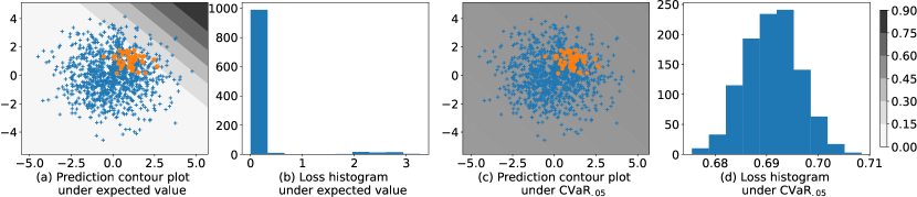
Figure 1: Prediction (predicted probability of a covariate being labeled as $1$) contours and loss histograms of two models learned under the expected loss and the $\textnormal{CVaR}_{.05}$ objective, respectively. The blue pluses and orange dots represent two classes. The loss distribution for the expected loss model has extremely high values for a small subset of the covariates.

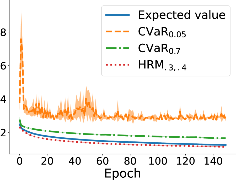
(a) Training objective values

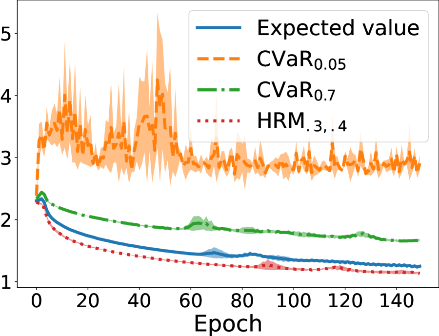
(b) Testing objective values

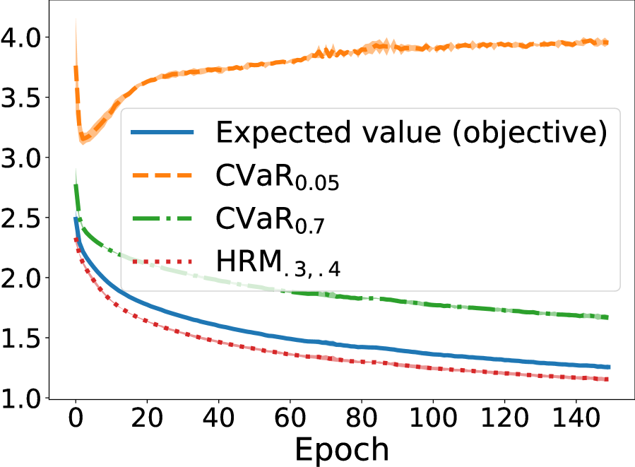
(c) Training risk evaluations

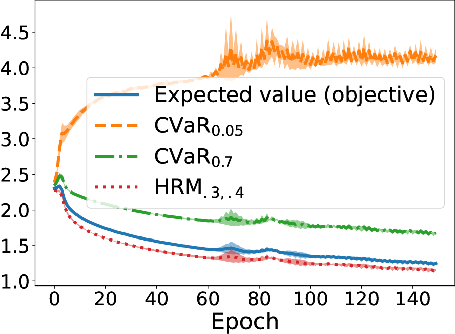
(d) Testing risk evaluations

Figure 2: Performance of VGG-16 models trained under expected loss, $\textnormal{CVaR}_{.05}$, $\textnormal{CVaR}_{.7}$ and $\text{HRM}_{.3,.4}$. In Figures 2(a) and 2(b), each model is trained and evaluated on the same objective. In Figures 2(c) and 2(d), we only train one model under the expected loss but report all four objectives of that model. All results are averaged over $5$ runs.

CIFAR-10

We have trained VGG-16 models on CIFAR-10 through minimizing the empirical risks for expected loss, $\textnormal{CVaR}_{.05}$, $\textnormal{CVaR}_{.7}$ and $\text{HRM}_{.3,.4}$ (Leqi et al., 2019) using the gradient descent step presented in (7). The models are trained over $150$ epochs and the learning rate is chosen to be $0.005$. As shown in Figure 2(a) and 2(b), in general, the objective values are decreasing over the epochs during training and testing. In addition, we observe that minimizing the empirical risk for expected loss does not necessarily imply minimizing other risks, e.g., $\textnormal{CVaR}_{.05}$ (Figure 2(c)). These results suggest the efficacy of our proposed optimization procedure for minimizing distortion risks.

8 Discussion

We have presented a principled framework, including analytic tools and algorithms for risk-sensitive learning and assessment that: (1) obtains the empirical CDF; (2) estimates the risks of interest through plugging in the empirical CDF; and (3) minimizes the empirical risk (for risk-sensitive learning). Our theoretical results on the uniform convergence of the proposed risk estimators hold simultaneously over a hypothesis class (constrained by an appropriate complexity measure) and over Hölder risks. The key building block for these results is the uniform convergence of the CDF estimator.

There are multiple future directions of our work. First, we hope to more precisely characterize the permutation complexity (under various hypothesis classes). Second, our gradient descent procedure (7) requires sorting all losses. An important next step would be to allow minibatches (sorting only a small subset of losses) when minimizing empirical distortion risks. Third, as shown in Figure 1, models learned under different risk objectives behave distinctly. Characterizing these model behaviors theoretically and empirically, and understanding the trade-offs among these objectives is crucial for building future models.

Appendix A Hölder Risk Functionals

In the definition of Hölder risk functionals, we require $d$ to be a quasi-metric, which we provide the definition here.

Definition A.1.

A function $d:\mathcal{L}_{\infty}(\mathbb{R},\mathbb{B}(\mathbb{R}))\times\mathcal{L}_{\infty}(\mathbb{R},\mathbb{B}(\mathbb{R}))\rightarrow[0,+\infty)$ is a quasi-metric if the following two conditions hold:

• For all $F_{U},F_{U^{\prime}}\in\mathcal{L}_{\infty}(\mathbb{R},\mathbb{B}(\mathbb{R}))$, $d(F_{U},F_{U^{\prime}})=0$ if and only if $F_{U}=F_{U^{\prime}}$;

• For all $F_{U},F_{U^{\prime}},F_{Z^{\prime\prime}}\in\mathcal{L}_{\infty}(\mathbb{R},\mathbb{B}(\mathbb{R}))$, $d(F_{U},F_{Z^{\prime\prime}})\leq d(F_{U},F_{U^{\prime}})+d(F_{U^{\prime}},F_{Z^{\prime\prime}})$.

If a quasimetric is symmetic, i.e., for all $F_{U},F_{U^{\prime}}\in\mathcal{L}_{\infty}(\mathbb{R},\mathbb{B}(\mathbb{R}))$, $d(F_{U},F_{U^{\prime}})=d(F_{U^{\prime}},F_{U})$, it is also a metric. The set of quasi-metrics contains symmetric quasi-metics, e.g., sup norms $\mathcal{L}_{\infty}$, Wasserstein distance, along with non-symmetric quasi-metrics, e.g., Kullback-Leibler divergence.

We will now discuss why optimized certainty equivalent (OCE) risks (e.g., mean-variance, entropic risk, CVaR) and spectral risks with bounded spectrum (e.g., CVaR, certain CPT-inspired Risks) are Lipschitz on bounded random variables. OCE risks, first introduced by Ben-Tal and Teboulle [1986], are defined as

$$\rho_{\text{oce}}(F_{U}):=\inf_{\lambda\in\mathbb{R}}\left\{\lambda+\mathbb{E}[\phi(U-\lambda)]\right\},$$

where $\phi:\mathbb{R}\to\mathbb{R}\cup\{+\infty\}$ is a nondecreasing, closed and convex function with $\phi(0)=0$ and $1\in\partial\phi(0)$. To complement the risk-averse OCEs, a risk-seeking version (inverted OCE) is proposed:

$$\rho_{\overline{{\text{oce}}}}(F_{U}):=\sup_{\lambda\in\mathbb{R}}\left\{\lambda-\mathbb{E}[\phi(\lambda-U)]\right\}.$$

Proposition A.1.

If $\phi$ is continuously differentiable, then the OCE risks $\rho_{\text{oce}}$ and inverted OCE risks $\rho_{\overline{{\text{oce}}}}$ are Lipschitz on the space of bounded random variables with support $[0,D]$:

$$|\rho_{\text{oce}}(F_{U})-\rho_{\text{oce}}(F_{U^{\prime}})| \leq\max_{x\in[0,D]}(\phi(D-x)-\phi(-x))\|F_{U}-F_{U^{\prime}}\|_{\infty},$$

$$|\rho_{\overline{{\text{oce}}}}(F_{U})-\rho_{\overline{{\text{oce}}}}(F_{U^{\prime}})| \leq\max_{x\in[0,D]}(\phi(x-D)-\phi(x))\|F_{U}-F_{U^{\prime}}\|_{\infty}.$$

Remark A.1.

Similar to Huang et al. [2021, Lemma 4.1], Proposition A.1 shows that the expected value and $\text{CVaR}_{\alpha}$ are $D$- and $\frac{D}{\alpha}$-Lipschtiz on random variables with support $[0,D]$, respectively. In addition, this result also provides Lipschitzness of the entropic risks (since the corresponding $\phi$ is continuously differentiable [Lee et al., 2020, Table 1]) and other OCE and inverted OCE risks that do not belong to distortion risk functionals.

Proof.

When $U$ has support $[0,D]$, as shown in Lee et al. [2020, Lemma 9], we can re-write the OCE and inverted OCE risks as follows:

$$\rho_{\text{oce}}(F_{U}) =\min_{\lambda\in[0,D]}\left\{\lambda+\mathbb{E}[\phi(U-\lambda)]\right\}$$

$$\rho_{\overline{{\text{oce}}}}(F_{U}) =\max_{\lambda\in[0,D]}\left\{\lambda-\mathbb{E}[\phi(\lambda-U)]\right\}.$$

For any $U,U^{\prime}\in[0,D]$, denote $\lambda_{U}\in\operatorname*{arg\,min}_{\lambda\in[0,D]}\lambda+\mathbb{E}_{U}[\phi(U-\lambda)]$ and $\lambda_{U^{\prime}}\in\operatorname*{arg\,min}_{\lambda\in[0,D]}\lambda+\mathbb{E}_{U^{\prime}}[\phi(U^{\prime}-\lambda)]$. Consider the case where $\rho_{\text{oce}}(F_{U})<\rho_{\text{oce}}(F_{U^{\prime}})$.

$$|\rho_{\text{oce}}(F_{U})-\rho_{\text{oce}}(F_{U^{\prime}})| =\rho_{\text{oce}}(F_{U^{\prime}})-\rho_{\text{oce}}(F_{U})$$

$$=\lambda_{U^{\prime}}+\mathbb{E}_{U^{\prime}}[\phi(U^{\prime}-\lambda_{U^{\prime}})]-\lambda_{U}-\mathbb{E}_{U}[\phi(U-\lambda_{U})]$$

$$\stackrel{{\scriptstyle(i)}}{{\leq}}\lambda_{U}+\mathbb{E}_{U^{\prime}}[\phi(U^{\prime}-\lambda_{U})]-\lambda_{U}-\mathbb{E}_{U}[\phi(U-\lambda_{U})]$$

$$=\int_{0}^{D}\phi(u-\lambda_{U})d\left(F_{U^{\prime}}(u)-F_{U}(u)\right)$$

$$\stackrel{{\scriptstyle(ii)}}{{=}}\phi(u-\lambda_{U})\left(F_{U^{\prime}}(u)-F_{U}(u)\right)\Big{|}_{u=0}^{u=D}-\int_{0}^{D}\phi^{\prime}(u-\lambda_{U})\left(F_{U^{\prime}}(u)-F_{U}(u)\right)du$$

$$\stackrel{{\scriptstyle(iii)}}{{\leq}}\|F_{U}-F_{U^{\prime}}\|_{\infty}\int_{0}^{D}\phi^{\prime}(u-\lambda_{U})du$$

$$=\left(\phi(D-\lambda_{U})-\phi(-\lambda_{U})\right)\|F_{U}-F_{U^{\prime}}\|_{\infty},$$

where $(i)$ comes from the definition of $\lambda_{U^{\prime}}$, $(ii)$ uses integration by parts, and $(iii)$ uses the fact that $\phi$ is non-decreasing, i.e., $\phi^{\prime}$ is non-negative, and $F_{U}(0)=F_{U^{\prime}}(0)=0,F_{U}(D)=F_{U^{\prime}}(D)=1$. The case when $\rho_{\text{oce}}(F_{U^{\prime}})<\rho_{\text{oce}}(F_{U})$ proceeds similarly:

$$|\rho_{\text{oce}}(F_{U})-\rho_{\text{oce}}(F_{U^{\prime}})| =\rho_{\text{oce}}(F_{U})-\rho_{\text{oce}}(F_{U^{\prime}})$$

$$\leq\int_{0}^{D}\phi(u-\lambda_{U^{\prime}})d\left(F_{U}(u)-dF_{U^{\prime}}(u)\right)$$

$$=\phi(u-\lambda_{U^{\prime}})\left(F_{U}(u)-F_{U^{\prime}}(u)\right)\Big{|}_{u=0}^{u=D}-\int_{0}^{D}\phi^{\prime}(u-\lambda_{U^{\prime}})\left(F_{U}(u)-F_{U^{\prime}}(u)\right)du$$

$$\leq\left(\phi(D-\lambda_{U^{\prime}})-\phi(-\lambda_{U^{\prime}})\right)\|F_{U}-F_{U^{\prime}}\|_{\infty}.$$

Putting it together, we have that

$$|\rho_{\text{oce}}(F_{U})-\rho_{\text{oce}}(F_{U^{\prime}})|\leq\max_{\lambda\in[0,D]}(\phi(D-x)-\phi(-x))\|F_{U}-F_{U^{\prime}}\|_{\infty}.$$

For inverted OCE risks, denote $\lambda_{U}\in\operatorname*{arg\,max}_{\lambda\in[0,D]}\lambda+\mathbb{E}_{U}[\phi(\lambda-U)]$ and $\lambda_{U^{\prime}}\in\operatorname*{arg\,max}_{\lambda\in[0,D]}\lambda+\mathbb{E}_{U^{\prime}}[\phi(\lambda-U)]$. The proof proceeds similarly by using the fact that $\rho_{\overline{{\text{oce}}}}(F_{U^{\prime}})-\rho_{\overline{{\text{oce}}}}(F_{U})\leq\mathbb{E}_{U}[\phi(\lambda_{U^{\prime}}-U)]-\mathbb{E}_{U^{\prime}}[\phi(\lambda_{U^{\prime}}-U^{\prime})]$ and $\rho_{\overline{{\text{oce}}}}(F_{U})-\rho_{\overline{{\text{oce}}}}(F_{U}^{\prime})\leq\mathbb{E}_{U^{\prime}}[\phi(\lambda_{U}-U^{\prime})]-\mathbb{E}_{U}[\phi(\lambda_{U}-U)]$. Following similar steps, we obtain that

$$|\rho_{\overline{{\text{oce}}}}(F_{U})-\rho_{\overline{{\text{oce}}}}(F_{U^{\prime}})|\leq\max_{\lambda\in[0,D]}(\phi(x-D)-\phi(x))\|F_{U}-F_{U^{\prime}}\|_{\infty}.$$

∎

Spectral risks (also known as $L$-risks or rank-weighted risks) are a subset of distortion risk functionals. As noted in Bäuerle and Glauner [2021], a spectral risk can be written as a distortion risk (Equation (4)) with the following distortion function: for $t\in[0,1]$,

$$g(t)=\int_{0}^{t}h(s)ds,$$

where $h:[0,1]\to\mathbb{R}_{+}$ is the non-decreasing spectrum function that integrates to $1$. Since $g$ is Lipschitz when $h$ is bounded (i.e., $g^{\prime}(t)=h(t)$ for $t\in(0,1)$), spectral risks are Lipschitz on the space of bounded random variables when their spectrum is bounded.

Finally, examples of risk functionals that are Hölder but are not Lipschitz include distortion risks whose distortion functions are Hölder but not Lipschitz.

Appendix B Proof of Results in Section 4

We note that in the following proofs, $Z$ is used to denote a generic random variable and the loss function is denoted by $\ell:\mathcal{X}\times\mathcal{Y}\times\mathcal{Y}\rightarrow\mathbb{R}$. (The loss function presented in the main text is a special case of this.) For a given $(X,Y,f(X))$, the loss is denoted by $\ell(X,Y,f(X))$.

B.1 Auxillary Lemmas

The below two auxillary lemmas are mainly adaptations to the class note from Professor Roberto Imbuzeiro Oliveira [Oliveira and Yang, ].

Lemma B.1.

Let $\mathbb{G}(1):=\left\{g(\cdot\;;r):=\mathbbm{1}_{\{\cdot\;\leq r\}}:\forall r\in\mathbb{R}\right\}$. For a fixed $f\in\mathbb{F}$, iid sample $\{X_{i},Y_{i}\}_{i=1}^{n}$ with joint probability measure $\mathbb{P}$, and a loss function $\ell:\mathcal{X}\times\mathcal{Y}\times\mathcal{Y}\rightarrow\mathbb{R}$, we have that

$$\sup_{g\in\mathbb{G}(1)}\left|\sum_{i=1}^{n}\xi_{i}g(\ell(X_{i},Y_{i},f(X_{i})))\right|=\max_{j\in[n]}\left|\sum_{i=1}^{j}\xi_{i}\right|,$$ (8)

and further

$$\mathbb{E}_{\mathbb{P},\mathfrak{R}}\left[\exp\left(\frac{\lambda}{n}\sup_{g\in\mathbb{G}(1)}\left|\sum_{i=1}^{n}\xi_{i}g(\ell(X_{i},Y_{i},f(X_{i})))\right|\right)\right]\leq 2\mathbb{E}_{\mathfrak{R}}\left[\max_{j\in[n]}\left(\exp\left(\frac{\lambda}{n}\sum_{i=1}^{j}\xi_{i}\right)\mathbbm{1}_{\{\sum_{i=1}^{j}\xi_{i}\geq 0\}}\right)\right].$$ (9)

Remark B.1.

We note that an important property of Lemma B.1 is that the bound is independent of the samples $\{X_{i},Y_{i}\}_{i=1}^{n}$.

Proof.

Let $\{R_{i}\}_{i=1}^{n}$ denote the sorted sequence of $\{\ell(X_{i},Y_{i},f(X_{i}))\}_{i=1}^{n}$, where $R_{1}\leq R_{2}\ldots\leq R_{n}$. Using $\{R_{i}\}_{i=1}^{n}$, we have

$$\mathbb{E}_{\mathbb{P},\mathfrak{R}}\left[\exp\left(\frac{\lambda}{n}\sup_{g\in\mathbb{G}(1)}\left|\sum_{i=1}^{n}\xi_{i}g(\ell(X_{i},Y_{i},f(X_{i})))\right|\right)\right]=\mathbb{E}_{\mathbb{P},\mathfrak{R}}\left[\exp\left(\frac{\lambda}{n}\sup_{g\in\mathbb{G}(1)}\left|\sum_{i=1}^{n}\xi_{i}g(R_{i})\right|\right)\right]$$

Consider a function $g(t;r)=\mathbbm{1}_{\{t\leq r\}}$. For such a function, $\sum_{i=1}^{n}\xi_{i}g(R_{i};r)$ is equal to

• $0$ if $r<\min_{i\in[n]}R_{i}$,

• $\sum_{i=1}^{j}\xi_{i}$ when $R_{j}\leq r<R_{j+1}$ for some $j\in\{1,\ldots,n-1\}$,

• $\sum_{i=1}^{n}\xi_{i}$ otherwise.

Therefore, we have that

$$\sup_{g\in\mathbb{G}(1)}\left|\sum_{i=1}^{n}\xi_{i}g(\ell(X_{i},Y_{i},f(X_{i})))\right|=\max_{j\in[n]}\left|\sum_{i=1}^{j}\xi_{i}\right|.$$

Finally, we notice that

$$\mathbb{E}_{\mathbb{P},\mathfrak{R}}\left[\sup_{g\in\mathbb{G}(1)}\exp\left(\frac{\lambda}{n}\left|\sum_{i=1}^{n}\xi_{i}g(R_{i})\right|\right)\right]=\mathbb{E}_{\mathbb{P},\mathfrak{R}}\left[\max_{j\in[n]}\exp\left(\frac{\lambda}{n}\left|\sum_{i=1}^{j}\xi_{i}\right|\right)\right]$$

$$= \mathbb{E}_{\mathbb{P},\mathfrak{R}}\Big{[}\max_{j\in[n]}\Big{(}\exp\left(\frac{\lambda}{n}\sum_{i=1}^{j}\xi_{i}\right)\mathbbm{1}_{\{\sum_{i=1}^{j}\xi_{i}\geq 0\}}+\exp\left(-\frac{\lambda}{n}\sum{i=1}^{j}\xi_{i}\right)\mathbbm{1}_{\{\sum_{i=1}^{j}\xi_{i}<0\}}\Big{)}\Big{]}$$

$$= \mathbb{E}_{\mathbb{P},\mathfrak{R}}\left[\max_{j\in[n]}\left(\exp\left(\frac{\lambda}{n}\sum_{i=1}^{j}\xi_{i}\right)\mathbbm{1}_{\{\sum_{i=1}^{j}\xi_{i}\geq 0\}}\right)\right]+\mathbb{E}_{\mathbb{P},\mathfrak{R}}\left[\max_{j\in[n]}\left(\exp\left(-\frac{\lambda}{n}\sum_{i=1}^{j}\xi_{i}\right)\mathbbm{1}_{\{\sum_{i=1}^{j}\xi_{i}<0\}}\right)\right]$$

$$\leq 2\mathbb{E}_{\mathbb{P},\mathfrak{R}}\left[\max_{j\in[n]}\left(\exp\left(\frac{\lambda}{n}\sum_{i=1}^{j}\xi_{i}\right)\mathbbm{1}_{\{\sum_{i=1}^{j}\xi_{i}\geq 0\}}\right)\right].$$ (10)

∎

Lemma B.2.

Let $\{Z_{i}\}_{i=1}^{n}$ taking values in $\mathcal{Z}$ denote independent samples drawn from $\mathbb{P}$ and $w:\mathcal{Z}\to\mathbb{R}_{+}$. For $n$ independent Rademacher random variables $\{\xi_{i}\}_{i=1}^{n}$, we have that for all $\lambda\geq 0$,

$$\mathbb{E}_{\mathbb{P},\mathfrak{R}}\left[\exp\left(\max_{j\in[n]}\frac{\lambda}{n}\sum_{i=1}^{j}w(Z_{i})\xi_{i}\right)\right]\leq 2\mathbb{E}_{\mathbb{P},\mathfrak{R}}\left[\exp\left(\frac{\lambda}{n}\sum_{i=1}^{n}w(Z_{i})\xi_{i}\right)\right].$$

Further, if $\frac{1}{n}\sum_{i=1}^{n}w(Z_{i})\xi_{i}$ is mean zero $\frac{\gamma^{2}}{n}$-subGaussian, then

$$\mathbb{E}_{\mathfrak{R}}\left[\exp\left(\max_{j\in[n]}\frac{\lambda}{n}\sum_{i}^{j}\xi_{i}\right)\right]\leq 2\exp\left(\frac{\lambda^{2}\gamma^{2}}{2n}\right).$$

Remark B.2.

We note that an immediate consequence of Lemma B.2 is

$$\mathbb{E}_{\mathbb{P},\mathfrak{R}}\left[\max_{j\in[n]}\left(\exp\left(\frac{\lambda}{n}\sum_{i=1}^{j}w(Z_{i})\xi_{i}\right)\mathbbm{1}_{\{\sum_{i=1}^{j}w(Z_{i})\xi_{i}\geq 0\}}\right)\right]$$

$$\leq \mathbb{E}_{\mathbb{P},\mathfrak{R}}\left[\exp\left(\max_{j\in[n]}\frac{\lambda}{n}\sum_{i=1}^{j}w(Z_{i})\xi_{i}\right)\right]\leq 2\mathbb{E}_{\mathbb{P},\mathfrak{R}}\left[\exp\left(\frac{\lambda}{n}\sum_{i=1}^{n}w(Z_{i})\xi_{i}\right)\right].$$

Proof.

The proof contains two main steps:
Step 1: We will show that for all $t>0$,

$$\mathbb{P}\left(\max_{j\in[n]}\sum_{i=1}^{j}w(Z_{i})\xi_{i}\geq t\right)\leq 2\mathbb{P}\left(\sum_{i=1}^{n}w(Z_{i})\xi_{i}\geq t\right).$$ (11)

To show (11), for $t>0$, consider events $E_{0}:=\emptyset$ and $E_{j}:=\{\sum_{i=1}^{j}w(Z_{i})\xi_{i}\geq t,\sum_{i=1}^{l}w(Z_{i})\xi_{i}<t,\forall l<j\}$ for $j\in[n]$, which states that $j$ is the first index such that the partial sum $\sum_{i=1}^{j}w(Z_{i})\xi_{i}$ is at least $t$. We first notice that

$$\left\{\max_{j}\sum_{i=1}^{j}w(Z_{i})\xi_{i}\geq t\right\}\subset\bigcup_{j=0}^{n}E_{j}.$$

Since $E_{j}$ and $\sum_{i=j+1}^{n}w(Z_{i})\xi_{i}\geq 0$ implies that $\sum_{i=1}^{n}w(Z_{i})\xi_{i}\geq t$, we obtain

$$\bigcup_{j=0}^{n}\left(E_{j}\bigcap\left\{\sum_{i=j+1}^{n}w(Z_{i})\xi_{i}\geq 0\right\}\right)\subset\left\{\sum_{i=1}^{n}w(Z_{i})\xi_{i}\geq t\right\}.$$ (12)

Moreover, for any $j\in[n]$, we have

$$\mathbb{P}\left(\sum_{i=j+1}^{n}w(Z_{i})\xi_{i}\geq 0\right)\geq\frac{1}{2},$$ (13)

since $\sum_{i=j+1}^{n}w(Z_{i})\xi_{i}$ is symmetic around $0$ (i.e., $\sum_{i=j+1}^{n}w(Z_{i})\xi_{i}\stackrel{{\scriptstyle d}}{{=}}-\sum_{i=j+1}^{n}w(Z_{i})\xi_{i}$) for all $i\in\{0,\ldots,n\}$. For any $j\in[n]$, since the event $E_{j}$ (dependeing on $\{w(Z_{i}),\xi_{i}\}_{i\leq j}$) is independent of $\{\sum_{i=j+1}^{n}w(Z_{i})\xi_{i}\geq 0\}$, we have

$$\mathbb{P}\left(E_{j}\bigcap\left\{\sum_{i=j+1}^{n}w(Z_{i})\xi_{i}\geq 0\right\}\right)=\mathbb{P}\left(E_{j}\right)\mathbb{P}\left(\sum_{i=j+1}^{n}w(Z_{i})\xi_{i}\geq 0\right)\geq\frac{\mathbb{P}\left(E_{j}\right)}{2}.$$

As a result, we have

$$\mathbb{P}\left(\sum_{i=1}^{n}w(Z_{i})\xi_{i}\geq t\right) \geq\mathbb{P}\left(\bigcup_{j=0}^{n}\left(E_{j}\bigcap\left\{\sum_{i=j+1}^{n}w(Z_{i})\xi_{i}\geq 0\right\}\right)\right)$$

$$=\sum_{j=0}^{n}\mathbb{P}\left(E_{j}\bigcap\left\{\sum_{i=j+1}^{n}w(Z_{i})\xi_{i}\geq 0\right\}\right)$$

$$\geq\sum_{j=1}^{n}\frac{\mathbb{P}\left(E_{j}\right)}{2}$$

$$\geq\frac{1}{2}\mathbb{P}\left(\max_{j\in[n]}\sum_{i=1}^{j}w(Z_{i})\xi_{i}\geq t\right),$$

where the first equality holds because for $i\neq j$, $E_{i}\cap E_{j}=\emptyset$, the first inequality follows from (12) and the last inequality comes from the union bound.

Step 2: For any differentiable $f$ and random variable $X$,

$$\mathbb{E}[f(X)\mathbbm{1}_{\{X\geq 0\}}] =\mathbb{E}\left[\left(f(0)+\int_{0}^{X}f^{\prime}(t)dt\right)\right]$$

$$=f(0)\mathbb{E}[\mathbbm{1}_{\{X\geq 0\}}]+\mathbb{E}\left[\int_{0}^{\infty}f^{\prime}(t)\mathbbm{1}_{\{X\geq t\}}dt\right]$$

$$=f(0)\mathbb{P}(X\geq 0)+\int_{0}^{\infty}f^{\prime}(t)\mathbb{P}(X\geq t)dt,$$ (14)

where the last equality follows from Fubini’s theorem. Putting it altogether, we have

$$\mathbb{E}_{\mathbb{P},\mathfrak{R}}\left[\exp\left(\max_{j\in[n]}\frac{\lambda}{n}\sum_{i=1}^{j}w(Z_{i})\xi_{i}\right)\right]$$

$$= 1+\lambda\int_{0}^{\infty}\exp\left(\lambda t\right)\mathbb{P}\left(\max_{j\in[n]}\frac{1}{n}\sum_{i=1}^{j}w(Z_{i})\xi_{i}\geq t\right)dt$$

$$\leq 1+2\lambda\int_{0}^{\infty}\exp\left(\lambda t\right)\mathbb{P}\left(\frac{1}{n}\sum_{i=1}^{n}w(Z_{i})\xi_{i}\geq t\right)dt$$

$$= 1+2\mathbb{E}_{\mathbb{P},\mathfrak{R}}\left[\left(\exp\left(\frac{\lambda}{n}\sum_{i=1}^{n}w(Z_{i})\xi_{i}\right)-1\right)\mathbbm{1}_{\{\sum_{i=1}^{n}w(Z_{i})\xi_{i}\geq 0\}}\right]$$

$$= 1+2\mathbb{E}_{\mathbb{P},\mathfrak{R}}\left[\exp\left(\frac{\lambda}{n}\sum_{i=1}^{n}w(Z_{i})\xi_{i}\right)\right]-2\mathbb{P}\left(\sum_{i=1}^{n}w(Z_{i})\xi_{i}\geq 0\right)$$

$$\leq 2\mathbb{E}_{\mathbb{P},\mathfrak{R}}\left[\exp\left(\frac{\lambda}{n}\sum_{i=1}^{n}w(Z_{i})\xi_{i}\right)\right],$$

where the first inequality follows from (11), the second equality uses (B.1) with $f(t)=e^{\lambda t}$ and $X=\max_{j\in[n]}\frac{1}{n}\sum_{i=1}^{j}w(Z_{i})\xi_{i}$, and the last inequality follows from (13). Finally, if $\frac{1}{n}\sum_{i=1}^{n}w(Z_{i})\xi_{i}$ is mean zero $\frac{\gamma^{2}}{n}$-subGaussian, then using the definition of a subGaussian random variable, we obtain

$$2\mathbb{E}_{\mathbb{P},\mathfrak{R}}\left[\exp\left(\frac{\lambda}{n}\sum_{i=1}^{n}w(Z_{i})\xi_{i}\right)\right]\leq 2\exp\left(\frac{\lambda^{2}\gamma^{2}}{2n}\right).$$

∎

B.2 Proof of Theorem 4.1

See 4.1

Proof.

We first analyze the sensitivity of the sup-norm of the CDF estimator over $\mathbb{F}$ and $\mathbb{G}(1)$. For a given two sets $\{x_{i},y_{i}\}_{i=1}^{n}$ and $\{x^{\prime}_{i},y^{\prime}_{i}\}_{i=1}^{n}$, which just differ in $j$’th entry, let

$$\widehat{F}_{1}(r;f):=\frac{1}{n}\sum_{i=1}^{n}\mathbbm{1}_{\{\ell(y_{i},f(x_{i}))\leq r\}}~{}\text{and},~{}\widehat{F}_{2}(r;f):=\frac{1}{n}\sum_{i=1}^{n}\mathbbm{1}_{\{\ell(y^{\prime}_{i},f(x^{\prime}_{i}))\leq r\}}$$

Then, if $\sup_{f\in\mathbb{F}}\sup_{r\in\mathbb{R}}\left|\widehat{F}_{1}(r;f)-F(r;f)\right|\geq\sup_{f\in\mathbb{F}}\sup_{r\in\mathbb{R}}\left|\widehat{F}_{2}(r;f)-F(r;f)\right|$, we have

$$\sup_{f\in\mathbb{F}}\sup_{r\in\mathbb{R}}\left|\widehat{F}_{1}(r;f)-F(r;f)\right|-\sup_{f\in\mathbb{F}}\sup_{r\in\mathbb{R}}\left|\widehat{F}_{2}(r;f)-F(r;f)\right|$$

$$=\sup_{f\in\mathbb{F}}\sup_{r\in\mathbb{R}}\left|\frac{1}{n}\sum_{i=1}^{n}\mathbbm{1}_{\{\ell(X_{i},y_{i},f(x_{i}))\leq r\}}-F(r;f)\right|-\sup_{f\in\mathbb{F}}\sup_{r\in\mathbb{R}}\left|\frac{1}{n}\sum_{i=1}^{n}\mathbbm{1}_{\{\ell(x_{i},y^{\prime}_{i},f(x^{\prime}_{i}))\leq r\}}-F(r;f)\right|$$

$$=\sup_{f\in\mathbb{F}}\sup_{r\in\mathbb{R}}\left|\frac{1}{n}\sum_{i=1}^{n}\mathbbm{1}_{\{\ell(x^{\prime}_{i},y^{\prime}_{i},f(x^{\prime}_{i}))\leq r\}}+\frac{1}{n}\left(\mathbbm{1}_{\{\ell(x_{j},y_{j},f(x_{j}))\leq r\}}-\mathbbm{1}_{\{\ell(x^{\prime}_{j},y^{\prime}_{j},f(x^{\prime}_{j}))\leq r\}}\right)-F(r;f)\right|$$

$$\quad\quad\quad\quad\quad\quad\quad\quad\quad\quad\quad\quad\quad\quad\quad\quad\quad\quad\quad\quad-\sup_{f\in\mathbb{F}}\sup_{r\in\mathbb{R}}\left|\frac{1}{n}\sum_{i=1}^{n}\mathbbm{1}_{\{\ell(x^{\prime}_{i},y^{\prime}_{i},f(x^{\prime}_{i}))\leq r\}}-F(r;f)\right|$$

$$=\sup_{f\in\mathbb{F}}\sup_{r\in\mathbb{R}}\frac{1}{n}\left|\mathbbm{1}_{\{\ell(x_{j},y_{j},f(x_{j}))\leq r\}}-\mathbbm{1}_{\{\ell(x^{\prime}_{j},y^{\prime}_{j},f(x^{\prime}_{j}))\leq r\}}\right|\leq\frac{1}{n}.$$

$$\left|\sup_{f\in\mathbb{F}}\sup_{r\in\mathbb{R}}\left|\widehat{F}_{1}(r;f)-F(r;f)\right|-\sup_{f\in\mathbb{F}}\sup_{r\in\mathbb{R}}\left|\widehat{F}_{2}(r;f)-F(r;f)\right|\right|$$

$$\quad\quad\quad\leq\sup_{f\in\mathbb{F}}\sup_{r\in\mathbb{R}}\frac{1}{n}\left|\mathbbm{1}_{\{\ell(x_{j},y_{j},f(x_{j}))\leq r\}}-\mathbbm{1}_{\{\ell(x^{\prime}_{j},y^{\prime}_{j},f(x^{\prime}_{j}))\leq r\}}\right|=\frac{1}{n}$$

This bound holds no matter what $j$ and what data set we choose. Using bounded difference inequality, i.e., McDiarmid’s inequality  [Boucheron et al., 2013], we have,

$$\mathbb{P}\left(\sup_{f\in\mathbb{F}}\sup_{r\in\mathbb{R}}\left|\widehat{F}(r;f)-F(r;f)\right|-\mathbb{E}_{\mathbb{P}}\left[\sup_{f\in\mathbb{F}}\sup_{r\in\mathbb{R}}\left|\widehat{F}(r;f)-F(r;f)\right|\right]\leq\sqrt{\frac{\log(\frac{1}{\delta})}{2n}}\right)$$ (15)

with probability at least $1-\delta$. Using a ghost sample set $\{X^{\prime}_{i},Y^{\prime}_{i}\}_{i=1}^{n}$ we have

$$\mathbb{E}_{\mathbb{P}}\left[\sup_{f\in\mathbb{F}}\sup_{r\in\mathbb{R}}\left|\widehat{F}(r;f)-F(r;f)\right|\right]$$

$$= \mathbb{E}_{\mathbb{P}}\left[\sup_{f\in\mathbb{F}}\sup_{r\in\mathbb{R}}\left|\frac{1}{n}\sum_{i=1}^{n}\mathbbm{1}_{\{\ell(X_{i},Y_{i},f(X_{i}))\leq r\}}-\mathbb{E}_{\mathbb{P}}\left[\frac{1}{n}\sum_{i=1}^{n}\mathbbm{1}_{\{\ell(X^{\prime}_{i},Y^{\prime}_{i},f(X^{\prime}_{i}))\leq r\}}\right]\right|\right]$$

$$= \mathbb{E}_{\mathbb{P}}\left[\sup_{f\in\mathbb{F}}\sup_{g\in\mathbb{G}(1)}\left|\frac{1}{n}\sum_{i=1}^{n}g(\ell(X_{i},Y_{i},f(X_{i})))-\mathbb{E}_{\mathbb{P}}\left[\frac{1}{n}\sum_{i=1}^{n}g(\ell(X^{\prime}_{i},Y^{\prime}_{i},f(X^{\prime}_{i})))\right]\right|\right]$$

$$= \mathbb{E}_{\mathbb{P}}\left[\sup_{f\in\mathbb{F}}\sup_{g\in\mathbb{G}(1)}\left|\frac{1}{n}\mathbb{E}_{\mathbb{P}}\left[\sum_{i=1}^{n}g(\ell(X_{i},Y_{i},f(X_{i})))-\sum_{i=1}^{n}g(\ell(X^{\prime}_{i},Y^{\prime}_{i},f(X^{\prime}_{i})))\Big{|}\sigma\left(\{X_{i},Y_{i}\}_{i=1}^{n}\right)\right]\right|\right]$$

$$\leq \mathbb{E}_{\mathbb{P}}\left[\sup_{f\in\mathbb{F}}\sup_{g\in\mathbb{G}(1)}\left|\frac{1}{n}\sum_{i=1}^{n}\left(g(\ell(X_{i},Y_{i},f(X_{i})))-g(\ell(X^{\prime}_{i},Y^{\prime}_{i},f(X^{\prime}_{i})))\right)\right|\right]$$

$$\leq \mathbb{E}_{\mathbb{P},\mathfrak{R}}\left[\sup_{f\in\mathbb{F}}\sup_{g\in\mathbb{G}(1)}\left|\frac{1}{n}\sum_{i=1}^{n}\xi_{i}\left(g(\ell(X_{i},Y_{i},f(X_{i})))-g(\ell(X^{\prime}_{i},Y^{\prime}_{i},f(X^{\prime}_{i})))\right)\right|\right]$$

$$\leq 2\mathbb{E}_{\mathbb{P},\mathfrak{R}}\left[\sup_{f\in\mathbb{F}}\sup_{g\in\mathbb{G}(1)}\left|\frac{1}{n}\sum_{i=1}^{n}\xi_{i}g(\ell(X_{i},Y_{i},f(X_{i})))\right|\right]=2\mathcal{R}(n,\mathbb{F}).$$ (16)

Putting (15) and (B.2) together concludes the proof. ∎

B.3 Permuation Complexity

We note that this proof, along with many other proofs for Section 4, is based on the machinery and techniques in Massart’s finite class Lemma [Massart, 2000] and DKW inequality in [Devroye et al., 2013].

See 4.2

Proof.

For a positive $\lambda$, we have,

$$\exp\left(\lambda\mathcal{R}(n,\mathbb{F})\right) =\exp\left(\frac{\lambda}{n}\mathbb{E}_{\mathbb{P},\mathfrak{R}}\left[\sup_{f\in\mathbb{F}}\sup_{g\in\mathbb{G}(1)}\left|\sum_{i=1}^{n}\xi_{i}g(\ell(X_{i},Y_{i},f(X_{i})))\right|\right]\right)$$

$$\leq\mathbb{E}_{\mathbb{P},\mathfrak{R}}\left[\exp\left(\frac{\lambda}{n}\sup_{f\in\mathbb{F}}\sup_{g\in\mathbb{G}(1)}\left|\sum_{i=1}^{n}\xi_{i}g(\ell(X_{i},Y_{i},f(X_{i})))\right|\right)\right]$$

$$\leq\mathbb{E}_{\mathbb{P},\mathfrak{R}}\left[\mathbb{E}_{\mathbb{P},\mathfrak{R}}\left[\exp\left(\frac{\lambda}{n}\sup_{f\in\mathbb{F}}\sup_{g\in\mathbb{G}(1)}\left|\sum_{i=1}^{n}\xi_{i}g(\ell(X_{i},Y_{i},f(X_{i})))\right|\right)\Big{|}\sigma\left(\{X_{i},Y_{i}\}_{i=1}^{n}\right)\right]\right]$$ (17)

For any $f\in\mathbb{F}$, let $\pi_{f}$ denote a permutation such that $\ell(X_{\pi_{f}(i)},Y_{\pi_{f}(i)},f(X_{\pi_{f}(i)}))\leq\ell(X_{\pi_{f}(j)},Y_{\pi_{f}(j)},f(X_{\pi_{f}(j)}))$ for any $i,j\in[n]$ and $i\leq j$. Therefore we have,

$$\sup_{g\in\mathbb{G}(1)}\left|\sum_{i=1}^{n}\xi_{i}g(\ell(X_{i},Y_{i},f(X_{i})))\right|=\sup_{g\in\mathbb{G}(1)}\left|\sum_{i=1}^{n}\xi_{\pi_{f}(i)}g(\ell(X_{\pi_{f}(i)},Y_{\pi_{f}(i)},f(X_{\pi_{f}(i)})))\right|$$

Consider a function $g(r^{\prime})=\mathbbm{1}_{\{r^{\prime}\leq r\}}$. For such a function, $\sum_{i=1}^{n}\xi_{\pi_{f}(i)}g(\ell(X_{\pi_{f}(i)},Y_{\pi_{f}(i)},f(X_{\pi_{f}(i)})))$ is equal to,

• $0$ if $r<\min_{i}\{\ell(X_{\pi_{f}(i)},Y_{\pi_{f}(i)},f(X_{\pi_{f}(i)}))\}_{i}^{n}$,

• $\sum_{i}^{j}\xi_{\pi_{f}(i)}$ when $\ell(X_{\pi_{f}(j)},Y_{\pi_{f}(j)},f(X_{\pi_{f}(j)}))\leq r<\ell(X_{\pi_{f}(j+1)},Y_{\pi_{f}(j+1)},f(X_{\pi_{f}(j+1)}))$ for a $j\in\{1,\ldots,n-1\}$,

• $\sum_{i}^{n}\xi_{\pi_{f}(i)}$ otherwise.

Using this property, we have,

$$\sup_{g\in\mathbb{G}(1)}\left|\sum_{i=1}^{n}\xi_{\pi_{f}(i)}g(\ell(X_{\pi_{f}(i)},Y_{\pi_{f}(i)},f(X_{\pi_{f}(i)})))\right|=\max_{j}\left|\sum_{i}^{j}\xi_{\pi_{f}(i)}\right|$$ (18)

Using this equality, we can further extend the Eq. B.3,

$$\exp\left(\lambda\mathcal{R}(n,\mathbb{F})\right) \leq\mathbb{E}_{\mathbb{P},\mathfrak{R}}\left[\mathbb{E}_{\mathbb{P},\mathfrak{R}}\left[\exp\left(\frac{\lambda}{n}\sup_{f\in\mathbb{F}}\max_{j}\left|\sum_{i}^{j}\xi_{\pi_{f}(i)}\right|\right)\Big{|}\sigma\left(\{X_{i},Y_{i}\}_{i=1}^{n}\right)\right]\right]$$

$$\leq\mathbb{E}_{\mathbb{P},\mathfrak{R}}\left[\mathbb{E}_{\mathbb{P},\mathfrak{R}}\left[\mathcal{N}_{\Pi}(\mathbb{F}_{\ell},\{X_{i},Y_{i}\}_{i=1}^{n})\exp\left(\frac{\lambda}{n}\max_{j}\left|\sum_{i}^{j}\xi_{i}\right|\right)\Big{|}\sigma\left(\{X_{i},Y_{i}\}_{i=1}^{n}\right)\right]\right]$$

$$\leq\mathcal{N}_{\Pi}(n,\mathbb{F}_{\ell},\mathbb{P})\mathbb{E}_{\mathbb{P},\mathfrak{R}}\left[\exp\left(\frac{\lambda}{n}\max_{j}\left|\sum_{i}^{j}\xi_{i}\right|\right)\right],$$ (19)

where the second inequality follows from the fact that effectively, there are at most $\mathcal{N}_{\Pi}(\mathbb{F}_{\ell},\{X_{i},Y_{i}\}_{i=1}^{n})$ number of $\pi_{f}$’s. Using the same derivation for (B.1) (Lemma B.1), we have

$$\exp\left(\lambda\mathcal{R}(n,\mathbb{F})\right) \leq 2\mathcal{N}_{\Pi}(n,\mathbb{F}_{\ell},\mathbb{P})\mathbb{E}_{\mathbb{P},\mathfrak{R}}\left[\max_{j}\left(\exp\left(\frac{\lambda}{n}\sum_{i}^{j}\xi_{i}\right)\mathbbm{1}_{\{\sum_{i}^{j}\xi_{i}\geq 0\}}\right)\right].$$

By Lemma B.2, we have

$$\exp\left(\lambda\mathcal{R}(n,\mathbb{F})\right) \leq 4\mathcal{N}_{\Pi}(n,\mathbb{F}_{\ell},\mathbb{P})\exp\left(\frac{\lambda^{2}}{2n}\right)$$

Now, taking the log from both sides, and dividing by $\lambda$, we have $\mathcal{R}(n,\mathbb{F})\leq\frac{\log(4\mathcal{N}_{\Pi}(n,\mathbb{F}_{\ell},\mathbb{P}))}{\lambda}+\frac{\lambda}{2n}.$ Choosing $\lambda=\sqrt{2n\log(2\mathcal{N}_{\Pi}(n,\mathbb{F}_{\ell},\mathbb{P}))}$, we obtain the final result

$$\mathcal{R}(n,\mathbb{F}) \leq\sqrt{\frac{\log(4\mathcal{N}_{\Pi}(n,\mathbb{F}_{\ell},\mathbb{P}))}{2n}}.$$

∎

See 4.1

Proof.

The result follows since when $|\mathbb{F}|<\infty$, $\mathcal{N}_{\Pi}(n,\mathbb{F}_{\ell},\mathbb{P})\leq|\mathbb{F}|$, i.e., we need at most one permutation function to sort the losses for each $f\in\mathbb{F}$.

∎

Appendix C Proof of Results in Section 5

See 5.1

Proof.

For all $\rho\in\mathbb{T}$, since $\rho$ is $L(\rho,1,\mathcal{L}_{\infty})$ Hölder, we have that $|\rho(F(\cdot;f))-\rho(\widehat{F}(\cdot;f))|\leq L(\rho,1,\mathcal{L}_{\infty})\|F-\widehat{F}\|_{\infty}$. The desired result then follows. ∎

The error of risk assessment can be bounded using distances other than the sup-norm, such as the Wasserstein distance. For two random variables $U$ and $U^{\prime}$ with bounded support $[0,D]$, the dual form of the Wasserstein distance $W_{1}(F_{U},F_{U^{\prime}})$ is given by [Vallender, 1974],

$$W_{1}(F_{U},F_{U^{\prime}})=\int_{0}^{D}|F_{U}(t)-F_{U^{\prime}}(t)|dt\leq D\|F_{U}-F_{U}\|_{\infty}.$$

This inequality suggests the following corollary.

Corollary C.1.

Under the setting of Theorem 5.1 where the loss has support $[0,D]$, with probability $1-\delta$, for all $\rho\in\mathbb{T}$, we have

$$\sup_{f\in\mathbb{F}}|\rho(F(\cdot;f))-\rho(\widehat{F}(\cdot;f))|\leq L(\rho,p,W_{1})D^{p}\epsilon^{p},$$

where $\mathbb{T}$ is the set of $L(\cdot,p,W_{1})$ Hölder risk functionals on the space of bounded random variables.

Proof.

For all $\rho\in\mathbb{T}$, since $\rho$ is $L(\rho,p,W_{1})$ Hölder, we have that $|\rho(F(\cdot;f))-\rho(\widehat{F}(\cdot;f))|\leq L(\rho,p,W_{1})W_{1}(F,\widehat{F})^{p}\leq L(\rho,p,W_{1})D^{p}\|F-\widehat{F}\|_{\infty}^{p}$. The desired result then follows. ∎

See 5.1

Proof.

As is shown in Huang et al. [2021, Lemma 4.1], $\rho$ is $L$-Lipschitz. Thus, directly applying Theorem 5.1 concludes the proof. ∎

Appendix D Proofs for results in Section 6

D.1 Proof of Lemma 6.1

Before proving Lemma 6.1, we first present two auxiliary lemmas.

Lemma D.1.

For any continuous function $g,h:\mathbb{R}^{d}\to\mathbb{R}$, $\min(g,h)$ and $\max(g,h)$ are continuous. Similarly, for any Lipschitz continuous function $g,h:\mathbb{R}^{d}\to\mathbb{R}$, $\min(g,h)$ and $\max(g,h)$ are Lipschitz continuous.

Proof.

Denote $f_{\min}=\min(g,h)$ and $f_{\max}=\max(g,h)$.
Continuity: We first consider the case when both $g$ and $h$ are continuous. Define $\overline{\Theta}=\{\theta\in\mathbb{R}^{d}:g(\theta)=h({\theta})\}$. For $\theta\notin\overline{\Theta}$, $f_{\min}$ and $f_{\max}$ are continuous since $g,h$ are continuous. Consider $\theta\in\overline{\Theta}$. For every $\epsilon>0$, there exists $\delta_{g},\delta_{h}>0$ such that for all $\theta^{\prime}\in\mathbb{R}^{d}$, $\|\theta-\theta^{\prime}\|\leq\epsilon\implies|g(\theta)-g(\theta^{\prime})|\leq\delta_{g},|h(\theta)-h(\theta^{\prime})|\leq\delta_{h}$. In addition, $f_{\min}(\theta)=g(\theta)=h(\theta)$, $f_{\max}(\theta)=g(\theta)=h(\theta)$ and $f_{\min}(\theta^{\prime})$, $f_{\max}(\theta^{\prime})$ can be either $g(\theta^{\prime})$ or $h(\theta^{\prime})$. Combining both facts gives us that $|f_{\min}(\theta)-f_{\min}(\theta^{\prime})|\leq\max(\delta_{g},\delta_{h})$ and $|f_{\max}(\theta)-f_{\max}(\theta^{\prime})|\leq\max(\delta_{g},\delta_{h})$.

Lipschitz Continuity: We next work with the case where both $g$ and $h$ are Lipschitz continuous. When $|f_{\max}(\theta)-f_{\max}(\theta^{\prime})|=|g(\theta)-h(\theta^{\prime})|,$ we have the following two cases:

1. $g(\theta)>h(\theta^{\prime})$: $|g(\theta)-h(\theta^{\prime})|=g(\theta)-h(\theta^{\prime})\leq g(\theta)-g(\theta^{\prime}),$ since $f_{\max}(\theta^{\prime})=h(\theta^{\prime})$.

2. $g(\theta)\leq h(\theta^{\prime})$: $|g(\theta)-h(\theta^{\prime})|=h(\theta^{\prime})-g(\theta)\leq h(\theta^{\prime})-h(\theta),$ since $f_{\max}(\theta)=g(\theta)$.

Since both $h$ and $g$ are Lipschitz continuous, we obtain that

$$|f_{\max}(\theta)-f_{\max}(\theta^{\prime})|{\leq}\max_{f\in\{g,h\}}|f(\theta)-f(\theta^{\prime})|\lesssim\|\theta-\theta^{\prime}\|,$$

showing that $f_{\max}$ is Lipschitz continuous. The proof completes with the fact that $\min(f,g)=-\max(-f,-g)$. ∎

Lemma D.2.

If $\{\ell_{\theta}(x_{j},y_{j})\}_{j=1}^{n}$ are Lipschitz continuous in $\theta$, then for all $i\in[n]$, $\ell_{\theta}(\pi_{\theta}(i))$, i.e., the $i$-th smallest loss evaluated using data points $\{x_{j},y_{j}\}_{j=1}^{n}$, is Lipschitz continuous in $\theta$.

Proof.

The key observation is that the $i$-th smallest loss can be defined as $\ell_{\theta}(\pi_{\theta}(i))=\min\{\max\{\ell_{\theta}(j):j\in J\}:J\subseteq[n],|J|=i\}.$ Since each $\ell_{\theta}(j)$ is Lipschitz continuous in $\theta$ and that for $j^{\prime}\in J$, $\max\{\ell_{\theta}(j):j\in J\}=\max\{\ell_{\theta}(j^{\prime}),\max\{\ell_{\theta}(j):j\in J\setminus\{j^{\prime}\}\}\}$, by Lemma D.1, we have $\max\{\ell_{\theta}(j):j\in J\}$ to be Lipschitz continuous in $\theta$. Similarly, since $\max\{\ell_{\theta}(j):j\in J\}$ is Lipschitz continuous in $\theta$, we have $\min\{\max\{\ell_{\theta}(j):j\in J\}:J\subseteq[n],|J|=i\}$ to be Lipschitz continuous. ∎

See 6.1

Proof.

Using Lemma D.2, we obtain that $\ell_{\theta}(\pi_{\theta}(i))$ is Lipschitz in $\theta\in\Theta$. Following from a classical result of Rademacher [Rockafellar and Wets, 2009, Theorem 9.60], i.e., a locally Lipschitz function is differentiable almost everywhere, we have that $\rho(\widehat{F}_{\theta})$ is differentiable almost everywhere. ∎

D.2 Local Convergence

The proofs for Corollary 6.1 are standard [Bottou et al., 2018], which we provide for completeness.

See 6.1

Proof.

For notation simplicity, we use $h(\theta)$ to denote $\rho(\widehat{F}_{\theta})$ and $g_{t}$ to denote $\nabla_{\theta}\rho(\widehat{F}_{\theta})$ when $\theta=\theta_{t}$. Since $h(\theta)$ is differentiable almost everywhere, following (7), the sequence $\{h(\theta_{t})\}_{t=1}^{T}$ will be differentiable almost surely. Since $h$ is $\beta$-smooth, we have that

$$h(\theta_{t+1})-h(\theta_{t})\leq\nabla_{\theta}h(\theta_{t})^{\top}(\theta_{t+1}-\theta_{t})+\frac{\beta}{2}\|\theta_{t+1}-\theta_{t}\|^{2}.$$

We denote the filtration for the stochastic process ${\{\theta_{t}\}}_{t=1}^{T}$ to be ${\{\mathcal{F}_{t}\}}_{t=1}^{T}$. Extending the above inequality, we have

$$h(\theta_{t+1})-h(\theta_{t})\leq\nabla_{\theta}h(\theta_{t})^{\top}(-\eta(g_{t}+w_{t}))+\frac{\beta}{2}\|-\eta(g_{t}+w_{t})\|^{2},$$

which suggests that

$$\mathbb{E}[h(\theta_{t+1})-h(\theta_{t})]\leq-\eta\nabla_{\theta}h(\theta_{t})^{\top}g_{t}+\eta^{2}\frac{\beta}{2}(\|g_{t}\|^{2}+d\sigma_{w}^{2}),$$

where $\sigma_{w}^{2}=1/d$ is the variance of $w_{t}$. Therefore, for the conditional expectation, we have

$$\mathbb{E}\left[h(\theta_{t+1})-h(\theta_{t})\Big{|}\mathcal{F}_{t}\right] \leq\mathbb{E}\left[-\eta\nabla_{\theta}h(\theta_{t})^{\top}g_{t}+\eta^{2}\frac{\beta}{2}(\|g_{t}\|^{2}+1)\Big{|}\mathcal{F}_{k}\right]$$

$$=-(\eta-\eta^{2}\frac{\beta}{2})\mathbb{E}\left[\|\nabla_{\theta}h(\theta_{t})\|^{2}\Big{|}\mathcal{F}_{t}\right]+\eta^{2}\frac{\beta}{2}.$$

Using the telescoping sum and law of total expectation, we obtain

$$\mathbb{E}\left[h(\theta_{T})-h(\theta_{1})\Big{|}\mathcal{F}_{1}\right] =\mathbb{E}\left[\sum_{t=1}^{T}h(\theta_{1})-h(\theta_{t-1})\Big{|}\mathcal{F}_{1}\right]\leq(\eta-\eta^{2}\frac{\beta}{2})\mathbb{E}\left[\sum_{t=1}^{T}-\|\nabla_{\theta}h(\theta_{t})\|^{2}\Big{|}\mathcal{F}_{1}\right]+T\eta^{2}\frac{\beta}{2}.$$ (20)

Use the fact that $h(\theta_{\star})\leq h(\theta_{T})$, we have $\mathbb{E}\left[h(\theta_{1})-h(\theta_{T})\right]\leq h(\theta_{1})-h(\theta_{\star})$, which implies

$$(\eta-\eta^{2}\frac{\beta}{2})\mathbb{E}\left[\sum_{t=1}^{T}\|\nabla_{\theta}h(\theta_{t})\|^{2}\right]\leq h(\theta_{1})-h(\theta_{\star})+T\eta^{2}\frac{\beta}{2}.$$

Plugging the learning rate $\eta={\frac{1}{\beta\sqrt{T}}}$, we have $\eta-\eta^{2}\frac{\beta}{2}={\frac{1}{\beta\sqrt{T}}}-{\frac{1}{2\beta{T}}}\geq{\frac{1}{\beta\sqrt{T}}}-{\frac{1}{2\beta\sqrt{T}}}\geq{\frac{1}{2\beta\sqrt{T}}}>0.$ Therefore we have

$$\frac{1}{2\beta\sqrt{T}}\mathbb{E}\left[\sum_{t=1}^{T}\|\nabla_{\theta}h(\theta_{t})\|^{2}\right]\leq h(\theta_{1})-h(\theta_{\star})+\frac{1}{2\beta}.$$

Rearranging the above inequality gives the result. ∎

Appendix E Additional Experimental Details

E.1 Risk Assessment on ImageNet Models

Figure 3 shows the CVaR of models presented in Table 1 under different $\alpha$’s. We note that $\textnormal{CVaR}_{\alpha}$ is the expected value above the top $100\alpha$ percent losses.

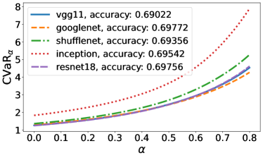
Figure 3: $\textnormal{CVaR}_{\alpha}(\ell_{f}(Z))$ across different $\alpha$’s where $\ell_{f}$ is the cross-entropy loss evaluated on the ImageNet validation dataset.

E.2 Empirical Distortion Risk Minimization

Toy Example

The data used in this experiment is generated using the make_blobs function from sklearn.datasets with the following parameters: n_samples = [1000, 50], centers = [[0.0, 0.0], [1.0, 1.0]], cluster_std = [1.5, 0.5], random_state = 0, shuffle = False.

References

- Acerbi [2002] Carlo Acerbi. Spectral measures of risk: A coherent representation of subjective risk aversion. Journal of Banking & Finance, 26(7):1505–1518, 2002.
- Alexander [1984] Kenneth S Alexander. Probability inequalities for empirical processes and a law of the iterated logarithm. The Annals of Probability, pages 1041–1067, 1984.
- Artzner et al. [1999] Philippe Artzner, Freddy Delbaen, Jean-Marc Eber, and David Heath. Coherent measures of risk. Mathematical finance, 9(3):203–228, 1999.
- Balbás et al. [2009] Alejandro Balbás, José Garrido, and Silvia Mayoral. Properties of distortion risk measures. Methodology and Computing in Applied Probability, 11(3):385–399, 2009.
- Bartlett and Mendelson [2002] Peter L Bartlett and Shahar Mendelson. Rademacher and gaussian complexities: Risk bounds and structural results. Journal of Machine Learning Research, 3(Nov):463–482, 2002.
- Bäuerle and Glauner [2021] Nicole Bäuerle and Alexander Glauner. Minimizing spectral risk measures applied to markov decision processes. Mathematical Methods of Operations Research, pages 1–35, 2021.
- Ben-Tal and Teboulle [1986] Aharon Ben-Tal and Marc Teboulle. Expected utility, penalty functions, and duality in stochastic nonlinear programming. Management Science, 32(11):1445–1466, 1986.
- Bhat and LA [2019] Sanjay P Bhat and Prashanth LA. Concentration of risk measures: A wasserstein distance approach. Advances in Neural Information Processing Systems, 32:11762–11771, 2019.
- Björk et al. [2014] Tomas Björk, Agatha Murgoci, and Xun Yu Zhou. Mean–variance portfolio optimization with state-dependent risk aversion. Mathematical Finance: An International Journal of Mathematics, Statistics and Financial Economics, 24(1):1–24, 2014.
- Bottou et al. [2018] Léon Bottou, Frank E Curtis, and Jorge Nocedal. Optimization methods for large-scale machine learning. Siam Review, 60(2):223–311, 2018.
- Boucheron et al. [2013] Stéphane Boucheron, Gábor Lugosi, and Pascal Massart. Concentration inequalities: A nonasymptotic theory of independence. Oxford university press, 2013.
- [12] Asaf Cassel, Shie Mannor, and Assaf Zeevi. A general framework for bandit problems beyond cumulative objectives.
- Chandak et al. [2021] Yash Chandak, Shiv Shankar, and Philip S. Thomas. High-confidence off-policy (or counterfactual) variance estimation, 2021.
- Denneberg [1990] Dieter Denneberg. Distorted probabilities and insurance premiums. Methods of Operations Research, 63(3):3–5, 1990.
- Devroye et al. [2013] Luc Devroye, László Györfi, and Gábor Lugosi. A probabilistic theory of pattern recognition, volume 31. Springer Science & Business Media, 2013.
- Duchi and Namkoong [2018] John Duchi and Hongseok Namkoong. Learning models with uniform performance via distributionally robust optimization. Annals of Statistics, 2018.
- Gänssler and Stute [1979] Peter Gänssler and Winfried Stute. Empirical processes: a survey of results for independent and identically distributed random variables. The Annals of Probability, pages 193–243, 1979.
- Gopalan et al. [2017] Aditya Gopalan, LA Prashanth, Michael Fu, and Steve Marcus. Weighted bandits or: How bandits learn distorted values that are not expected. In Proceedings of the AAAI Conference on Artificial Intelligence, volume 31, 2017.
- Guide [2006] A Hitchhiker’s Guide. Infinite dimensional analysis. Springer, 2006.
- He et al. [2016] Kaiming He, Xiangyu Zhang, Shaoqing Ren, and Jian Sun. Deep residual learning for image recognition. In Proceedings of the IEEE conference on computer vision and pattern recognition, pages 770–778, 2016.
- Holland and Haress [2021] Matthew J Holland and El Mehdi Haress. Spectral risk-based learning using unbounded losses. arXiv preprint arXiv:2105.04816, 2021.
- Huang et al. [2021] Audrey Huang, Liu Leqi, Zachary C Lipton, and Kamyar Azizzadenesheli. Off-policy risk assessment in contextual bandits. arXiv preprint arXiv:2104.08977, 2021.
- Jie et al. [2018] Cheng Jie, LA Prashanth, Michael Fu, Steve Marcus, and Csaba Szepesvári. Stochastic optimization in a cumulative prospect theory framework. IEEE Transactions on Automatic Control, 63(9):2867–2882, 2018.
- Khim et al. [2020] Justin Khim, Liu Leqi, Adarsh Prasad, and Pradeep Ravikumar. Uniform convergence of rank-weighted learning. In International Conference on Machine Learning, pages 5254–5263. PMLR, 2020.
- Krokhmal [2007] Pavlo A Krokhmal. Higher moment coherent risk measures. 2007.
- Kusuoka [2001] Shigeo Kusuoka. On law invariant coherent risk measures. In Advances in mathematical economics, pages 83–95. Springer, 2001.
- Lee et al. [2020] Jaeho Lee, Sejun Park, and Jinwoo Shin. Learning bounds for risk-sensitive learning. In 34th Conference on Neural Information Processing Systems (NeurIPS) 2020. Neural Information Processing Systems, 2020.
- Leqi et al. [2019] Liu Leqi, Adarsh Prasad, and Pradeep Ravikumar. On human-aligned risk minimization. In Advances in Neural Information Processing Systems, 2019.
- Li et al. [2020] Tian Li, Ahmad Beirami, Maziar Sanjabi, and Virginia Smith. Tilted empirical risk minimization. In International Conference on Learning Representations, 2020.
- Ma et al. [2018] Ningning Ma, Xiangyu Zhang, Hai-Tao Zheng, and Jian Sun. Shufflenet v2: Practical guidelines for efficient cnn architecture design. In Proceedings of the European conference on computer vision (ECCV), pages 116–131, 2018.
- Massart [1990] Pascal Massart. The tight constant in the dvoretzky-kiefer-wolfowitz inequality. The annals of Probability, pages 1269–1283, 1990.
- Massart [2000] Pascal Massart. Some applications of concentration inequalities to statistics. In Annales de la Faculté des sciences de Toulouse: Mathématiques, volume 9, pages 245–303, 2000.
- Munos [2014] Rémi Munos. From bandits to monte-carlo tree search: The optimistic principle applied to optimization and planning. 2014.
- [34] Lecturer: Prof Roberto Oliveira and Scribes: Shangjie Yang. Topics in statistical mathematics: Lecture 2. https://w3.impa.br/~rimfo/estatistica_a16/notas_alunos/shangjie.pdf. Accessed: 2021-9-15.
- Prashanth et al. [2016] LA Prashanth, Cheng Jie, Michael Fu, Steve Marcus, and Csaba Szepesvári. Cumulative prospect theory meets reinforcement learning: Prediction and control. In International Conference on Machine Learning, pages 1406–1415. PMLR, 2016.
- Rockafellar and Wets [2009] R Tyrrell Rockafellar and Roger J-B Wets. Variational analysis, volume 317. Springer Science & Business Media, 2009.
- Rockafellar et al. [2000] R Tyrrell Rockafellar, Stanislav Uryasev, et al. Optimization of conditional value-at-risk. Journal of risk, 2:21–42, 2000.
- Russakovsky et al. [2015] Olga Russakovsky, Jia Deng, Hao Su, Jonathan Krause, Sanjeev Satheesh, Sean Ma, Zhiheng Huang, Andrej Karpathy, Aditya Khosla, Michael Bernstein, Alexander C. Berg, and Li Fei-Fei. ImageNet Large Scale Visual Recognition Challenge. International Journal of Computer Vision (IJCV), 115(3):211–252, 2015. doi: 10.1007/s11263-015-0816-y.
- Sani et al. [2013] Amir Sani, Alessandro Lazaric, and Rémi Munos. Risk-aversion in multi-armed bandits. arXiv preprint arXiv:1301.1936, 2013.
- Shapiro et al. [2014] Alexander Shapiro, Darinka Dentcheva, and Andrzej Ruszczyński. Lectures on stochastic programming: modeling and theory. SIAM, 2014.
- Sharpe [1966] William F Sharpe. Mutual fund performance. The Journal of business, 39(1):119–138, 1966.
- Simonyan and Zisserman [2014] Karen Simonyan and Andrew Zisserman. Very deep convolutional networks for large-scale image recognition. arXiv preprint arXiv:1409.1556, 2014.
- Szegedy et al. [2015] Christian Szegedy, Wei Liu, Yangqing Jia, Pierre Sermanet, Scott Reed, Dragomir Anguelov, Dumitru Erhan, Vincent Vanhoucke, and Andrew Rabinovich. Going deeper with convolutions. In Proceedings of the IEEE conference on computer vision and pattern recognition, pages 1–9, 2015.
- Szegedy et al. [2016] Christian Szegedy, Vincent Vanhoucke, Sergey Ioffe, Jon Shlens, and Zbigniew Wojna. Rethinking the inception architecture for computer vision. In Proceedings of the IEEE conference on computer vision and pattern recognition, pages 2818–2826, 2016.
- Torossian et al. [2019] Léonard Torossian, Aurélien Garivier, and Victor Picheny. -armed bandits: Optimizing quantiles, cvar and other risks. In Asian Conference on Machine Learning, pages 252–267. PMLR, 2019.
- Vakili and Zhao [2015] Sattar Vakili and Qing Zhao. Mean-variance and value at risk in multi-armed bandit problems. In 2015 53rd Annual Allerton Conference on Communication, Control, and Computing (Allerton), pages 1330–1335. IEEE, 2015.
- Vallender [1974] SS Vallender. Calculation of the wasserstein distance between probability distributions on the line. Theory of Probability & Its Applications, 18(4):784–786, 1974.
- Vapnik [2006] Vladimir Vapnik. Estimation of dependences based on empirical data. Springer Science & Business Media, 2006.
- Vapnik [2013] Vladimir Vapnik. The nature of statistical learning theory. Springer science & business media, 2013.
- Vapnik [1999] Vladimir Naumovich Vapnik. An overview of statistical learning theory. IEEE transactions on neural networks, 10(5):988–999, 1999.
- Wainwright [2019] Martin J Wainwright. High-dimensional statistics: A non-asymptotic viewpoint, volume 48. Cambridge University Press, 2019.
- Wang [1996] Shaun Wang. Premium calculation by transforming the layer premium density. ASTIN Bulletin: The Journal of the IAA, 26(1):71–92, 1996.
- Wang et al. [1997] Shaun S Wang, Virginia R Young, and Harry H Panjer. Axiomatic characterization of insurance prices. Insurance: Mathematics and economics, 21(2):173–183, 1997.
- Wirch and Hardy [2001] Julia L Wirch and Mary R Hardy. Distortion risk measures: Coherence and stochastic dominance. In International congress on insurance: Mathematics and economics, pages 15–17, 2001.
- Wirch and Hardy [1999] Julia Lynn Wirch and Mary R Hardy. A synthesis of risk measures for capital adequacy. Insurance: mathematics and Economics, 25(3):337–347, 1999.
- Zimin et al. [2014] Alexander Zimin, Rasmus Ibsen-Jensen, and Krishnendu Chatterjee. Generalized risk-aversion in stochastic multi-armed bandits. arXiv preprint arXiv:1405.0833, 2014.