The intrinsic Fano factor of nuclear recoils for dark matter searches

Abstract

Nuclear recoils in germanium and silicon are shown to have much larger variance in electron-hole production than their electron-recoil counterparts for recoil energies between 10 and 200 keV. This effect–owing primarily to deviations in the amount of energy given to the crystal lattice in response to a nuclear recoil of a given energy–has been predicted by the Lindhard model. We parameterize the variance in terms of an intrinsic nuclear recoil Fano factor which is 24.3$\pm$0.2 and 26$\pm$8 at around 25 keV for silicon and germanium respectively. The variance has important effects on the expected signal shapes for experiments utilizing low-energy nuclear recoils such as direct dark matter searches and coherent neutrino-nucleus scattering measurements.

I Introduction

One of the most intensely researched channels for direct detection of dark matter is scattering off of a nucleus in a target material Arnaud et al. (2018); Abdelhameed et al. (2019); Angloher et al. (2014); Aprile et al. (2018); Agnese et al. (2018). While the ionization distribution for these recoils has never been well understood in solids, the Lindhard model Lindhard et al. (1963a) provides a benchmark. Experiments that simultaneously measured two deposition channels (like ionization and heat) did not worry about the exact ionization distributions in the past because they could measure recoil energy directly Armengaud et al. (2019); Agnese et al. (2015) (without a model for ionization production). With the two-channel measurements (ionization and heat) the results of dark matter searches was not systematically limited due to the lack of knowledge on the ionization.

In recent years, there has been a dramatic improvement in the detection energy threshold of many experiments Agnese et al. (2019); Aguilar-Arevalo et al. (2020), due largely to improvements in the measurement resolution for ionization or heat individually. The best detectors of the new generation of low-mass dark-matter-seeking experiments have single electron-hole pair sensitivity Tiffenberg et al. (2017); Romani et al. (2018). These detectors have not yet been able to achieve the ionization-yield insensitivity that their higher-energy predecessors have, so the dark-matter signal depends sensitively on the ionization yield and ionization variance produced by a low-energy nuclear recoil. In fact, it is often true that dominant systematic uncertainties in dark matter limits come from the uncertainty in the ionization yield Agnese et al. (2019). For single electron-hole devices the ionization variance also becomes a driving factor in the accuracy of signal models for low-mass dark matter via nuclear scattering.

While much of the literature has focused on the ionization yield Villano et al. (2022); Scholz et al. (2016); Chavarria et al. (2016); Sorensen (2015), there are existing published data that constrain the ionization variance either directly or indirectly Dougherty (1992); Gerbier et al. (1990); Martineau et al. (2004). And there is even more data still that might be used to more precisely measure the ionization variance if a resolution model was published Agnese et al. (2014).

We report here on the best such existing data to constrain the ionization variance in silicon and germanium, and provide a procedure by which such information can be extracted from a dark matter detector that measures two channels like ionization and heat. While our constraints are limited to the recoil energy region above about 24 keV, the techniques give insight into how this information can be extracted to lower energies in the future and the basic size and trend of the ionization variance for nuclear recoils.

To analyze the silicon data we have taken note that two previous publications have reported an “excess” ionization variance beyond the expected instrumental variance. We converted that variance into a Fano factor by using $\sigma_{e}^{2}$/$\bar{N}$=$F$, where $\sigma_{e}$ is the excess width in the ionization measurement.

We have used a similar method for a previous germanium publication. There, we used electron recoils to constrain the instrumental resolutions, obtaining an excellent fit to the measured widths for electron recoils (see Fig. 2). This instrumental resolution does not predict the nuclear recoil widths, so we include an “excess” variance in the form of a nuclear recoil Fano factor to obtain good fits. The method is similar to that of scintillator references Bousselham et al. (2010) who have accounted for instrumental resolution in order to obtain information on the intrinsic optical photon production process. The key difference being that the result in that publication shows sub-Poisson fluctuations in optical photon production where we see larger-than-Poisson fluctuations in electron-hole pair production for nuclear recoils.

Our results for the intrinsic nuclear recoil Fano factors of silicon and germanium (see Figs.1 and 6) are not in line with a division of some theoretical predictions of the electron recoil Fano factor Mei et al. (2020) by the ionization yield; this naive modification gives $F\sim$0.41. Those predictions, however, assume an underlying phonon distribution that is Poisson. Our results are roughly in line with the Lindhard Lindhard et al. (1963a) predictions which do not make that assumption.

II The Fano factor

The ionization variance for electron recoils is very succinctly characterized in terms of the Fano factor, F Fano (1946). Given an average number of electron-hole pairs produced, $\bar{N}$, the variance in this number of pairs is given simply by:

$$\sigma_{N}^{2}=F\bar{N}.$$ (1)

While this specification does not give insight into moments of the $N$ distribution of higher order than the variance, it emphasizes that $F$=1 corresponds to a behavior that is qualitatively similar to a Poisson distribution in the lowest two moments. For these reasons we find it simple and convenient to parameterize the nuclear recoil ionization variance in the same way, but with a modified intrinsic Fano factor, $F_{\mathrm{nr}}$ . The Fano factor for electron recoils seems to be in the range 0.084 – 0.16 Yamaya et al. (1979); Eberhardt (1970); Palms et al. (1969), but may have a temperature and/or energy dependence Perotti and Fiorini (1999). It is even possible that the “true” intrinsic Fano factor has not yet been measured directly and is lower than all the above measurements Zulliger and Aitken (1970).

In silicon there are two studies that we are aware of that measured the ionization variance in addition to the ionization yield for nuclear recoils. Both were done in the early 1990’s with secondary neutron beams produced from primary proton beams via the reaction ⁷Li(p,n)⁷Be Dougherty (1992); Gerbier et al. (1990). The measurement by Dougherty makes use of neutron elastic-scattering resonances present in silicon. The Gerbier et al. measurement uses a fixed-angle secondary neutron detector and a timing coincidence to constrain the true recoil energy in the silicon scattering detector.

Both of these measurements report the “extra” ionization variance after subtracting the expected variance due to known sources of errors such as instrumental noise or angular uncertainty in the secondary neutron scatters. The extracted additional ionization variance can be compared with the total recoil energy (inferred in the Dougherty measurement and measured in the Gerbier measurement) to give what we will define as the intrinsic fractional ionization width, $\xi$. This fractional ionization width is defined as the ionization width (in energy units) divided by the ionization energy collected, so that $\xi=\sigma_{N}/\bar{N}$. With these definitions the intrinsic nuclear-recoil Fano factor, $F_{\mathrm{nr}}$, is given by:

$$F_{\mathrm{nr}}=\bar{N}\xi^{2}=\frac{E_{r}\bar{Q}}{\epsilon_{\gamma}}\xi^{2},$$ (2)

where $E_{r}$ is the true recoil energy, $\bar{Q}$ is the average ionization yield (ratio of “collected” ionization energy to total energy; unity for electron recoils), and $\epsilon_{\gamma}$ is the average energy to produce one electron-hole pair for an electron recoil.

Recoil Energy (keV)	Ion. Efficiency (%)	Non-instr. Width (eV)	Non-instr. Width (%)	Effective Fano	Reference
109.1$\pm$0.7	51.4$\pm$2	-	6.1$\pm$1.2	208$\pm$82	Dougherty Dougherty (1992)
75.7 $\pm$0.4	45.6$\pm$0.5	-	5.3$\pm$0.6	123$\pm$28	Dougherty Dougherty (1992)
25.3$\pm$0.3	35.5$\pm$0.6	-	3.6$\pm$0.3	24.3$\pm$4.1	Dougherty Dougherty (1992)
7.50$\pm$0.03	26.9$\pm$0.4	-	2.8$\pm$0.4	5.75$\pm$1.65	Dougherty Dougherty (1992)
4.15$\pm$0.15	22.5$\pm$0.5	-	2.2$\pm$0.9	2.35$\pm$1.92	Dougherty Dougherty (1992)
21.7$\pm$0.2	40.7$\pm$0.5	1000$\pm$59	-	29.80$\pm$17.11	Gerbier Gerbier et al. (1990)
19.5$\pm$0.2	38.7$\pm$0.7	1101$\pm$108	-	42.27$\pm$8.33	Gerbier Gerbier et al. (1990)
13.5$\pm$0.3	33.6$\pm$0.7	601$\pm$42	-	20.96$\pm$2.96	Gerbier Gerbier et al. (1990)
8.6$\pm$0.1	31.1$\pm$0.5	348$\pm$13	-	11.91$\pm$0.91	Gerbier Gerbier et al. (1990)
4.7$\pm$0.1	26.6$\pm$0.8	185$\pm$36	-	7.20$\pm$2.81	Gerbier Gerbier et al. (1990)
4.15$\pm$0.1	27.4$\pm$0.8	166$\pm$39	-	6.38$\pm$3.00	Gerbier Gerbier et al. (1990)
3.9$\pm$0.1	22.9$\pm$2.0	241$\pm$66	-	17.11$\pm$9.49	Gerbier Gerbier et al. (1990)
3.3$\pm$0.1	25.9$\pm$1.6	131$\pm$55	-	5.28$\pm$4.45	Gerbier Gerbier et al. (1990)

Table 1: Data from the past publications constraining the intrinsic Fano factor in silicon Dougherty (1992); Gerbier et al. (1990). The intrinsic Fano factor is calculated from Eq. 2 in the text, using the measurements of the non-instrumental widths and the ionization efficiency (yield).

Table 1 shows the resulting intrinsic nuclear-recoil Fano factors for the silicon nuclear recoils measured in the two references we have been discussing. Even at low recoil energies, around 3 keV, the intrinsic Fano factors show that the ionization variance is such that the number of created pairs have more variance than a Poisson process with the same average number of pairs.

The Lindhard et al. model, articulated in the early papers Lindhard et al. (1968, 1963b, 1963a); Lindhard and Scharff (1961), contains predictions for the variance in the production of electron-hole pairs in a solid medium in addition to the average ionization (ionization yield). We compare this theoretical ionization variance with “extra” ionization variance extracted by Dougherty and Gerbier as a possible explanation.

Figure 1 shows the ionization variance results of the previous measurements by Dougherty and Gerbier cast in terms of the intrinsic nuclear recoil Fano factor. Lindhard’s predictions–shown in terms of the intrinsic Fano factor–are also shown on the plot. The predictions shown employ two different approximations used in the Lindhard work: the approximate separability between electronic and nuclear energy deposits (referred to as approximation D); and the additional assumption of forward-scattering dominance in nuclear collisions (referred to as Approximation E). Approximation E produces a lower ionization yield and a larger ionization variance. The lower ionization yield for Approximation E is expected because in that case nuclear collisions are assumed to transfer small amounts of energy and therefore contribute a smaller fraction of their energy to ionization. Furthermore, the larger ionization variance is a consequence of the approximate proportionality between $F_{\mathrm{nr}}$ and $\sqrt{\epsilon}$, where $\epsilon$ is the average energy needed to create a single electron-hole pair Mei et al. (2020)–a quantity that increases with decreasing yield.

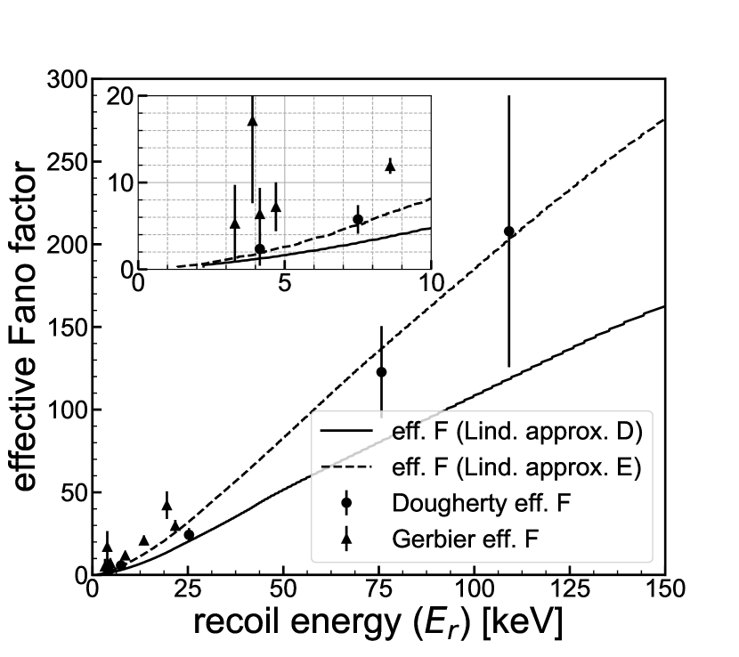
Figure 1: The measurements of Dougherty Dougherty (1992) and Gerbier Gerbier et al. (1990) converted into the intrinsic Fano factor for nuclear recoils. We also show the predictions of Lindhard Lindhard et al. (1963a) in the so-called Approximation D (solid) and Approximation E (dashed) curves (see text for descriptions). The inset shows a zoom of the low-energy region below 10 keV in recoil energy.

Despite clear evidence for a very large ionization production variance for nuclear recoils, and the importance of this variance for low-mass dark matter searches, studies of this effect are scant. Dark matter collaborations like SuperCDMS and EDELWEISS have excellent sensitivity to this effect because of their direct measurements of ionization yield. In the next sections we argue that the large ionization variance expected in moderate-energy nuclear recoils produces larger-than-expected measured ionization yield widths in cryogenic semiconductor detectors, and that this fact can be used to measure the ionization variance for silicon or germanium.

III Previous germanium ionization yield measurement

While the previously discussed measurements of the ionization variance in silicon came in the early 1990’s, other technologies that came later had excellent means to probe the ionization variance in germanium. Two such similar technologies came out of the cryogenic dark matter searches of EDELWEISS and SuperCDMS Martineau et al. (2004); Agnese et al. (2014).

EDELWEISS Martineau et al. (2004) was possibly the first to note in published work that the nuclear-recoil band in cryogenic ionization/phonon devices is expected to be significantly narrower than the electron-recoil band if only the effects of sensor resolution are included. Recently, the narrowness of the nuclear-recoil band when using empirical resolution functions has also been noted in the SuperCDMS detectors Kennedy (2017). The width of the nuclear-recoil band is directly related to the variance of the ionization yield (or what EDELWEISS and some others call the “Quenching”). In this work we use $Q$ to denote the random variable corresponding to the measured ionization yield for an event, and $\bar{Q}$ to denote the average of that quantity, equivalent to the $\langle Q\rangle$ of EDELWEISS.

At a given recoil energy the width of the quenching measurement was estimated in the 2004 EDELWEISS work Martineau et al. (2004) by :

$$\left(\sigma^{\mathrm{EDW}}_{\mathrm{NR}}\right)^{2}=\frac{1}{E_{r}^{2}}\left((1+\frac{V}{\epsilon_{\gamma}}\bar{Q})^{2}\sigma_{I}^{2}\\ +(1+\frac{V}{\epsilon_{\gamma}})^{2}\bar{Q}^{2}\sigma_{H}^{2}\right),$$ (3)

where $\sigma_{I}^{2}$ is the variance in the ionization signal in energy units and $\sigma_{H}^{2}$ is the variance in the heat signal in energy units. Since the quenching factor (less than unity for nuclear recoils) decreases each term in the equation, it is easy to see the variance in the event-by-event measured quenching should be significantly less for nuclear recoils than for electron recoils. In fact, this is not the case. EDELWEISS measures the variance in the nuclear recoils to be comparable to that of the electron recoils Martineau et al. (2004). We have reproduced the EDELWEISS analysis by first computing the expected ionization yield width for electron recoils and then doing a simple fit to constrain how much larger the nuclear recoil width that EDELWEISS measures is from the prediction in Eq. 3.

For the electron recoils, the average ionization yield, $\bar{Q}$, is taken to be unity. EDELWEISS parameterized the energy-dependent sensor resolutions by the following functional forms Martineau et al. (2004):

$$\sigma_{I}(E) =\sqrt{(\sigma_{I}^{0})^{2}+(a_{I}E)^{2}}$$ (4)

$$\sigma_{H}(E) =\sqrt{(\sigma_{H}^{0})^{2}+(a_{H}E)^{2}},$$

where $a_{I}$ and $a_{H}$ are adjustable parameters used to “tune” the ionization yield width. Using these resolutions we can compute the exact ionization yield width as a function of energy . The resolutions can also be used to calculate the nuclear-recoil width given an intrinsic Fano factor for nuclear recoils. The calculations are outlined in the Appendix.

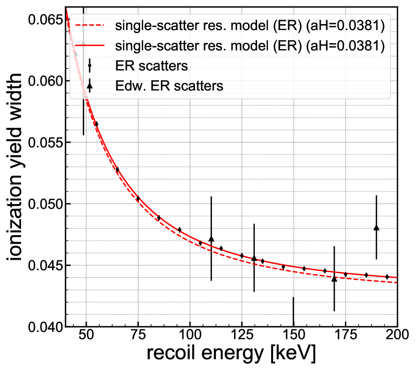
Figure 2: (Color online) The measured ionization width for electron recoils. The triangular data points are from the EDELWEISS Martineau et al. (2004) measurement on detector GGA3, and the circular data points are our simulation of that measurement with the “tuned” resolutions (see text). The solid curve is our exact model ($\sigma_{\mathrm{ER}}$) for the ionization width given the appropriate resolution and the dashed curve is the zeroth-order model ($\sigma^{\mathrm{EDW}}_{\mathrm{ER}}$) used by EDELWEISS.

Figure 2 shows the energy dependence of our exact expression for the electron-recoil width (see the Appendix) with the EDELWEISS approximations (Eq. 3). Looking at the electron-recoil band of the EDELWEISS GGA3 detector, we tune the parameter $a_{H}$ to be 0.0381 in FWHM units . This value gives the best fit to the EDELWEISS electron-recoil yield widths as a function of energy, as shown in Fig. 2. Also in the figure we have displayed the widths resulting from a simulation of these distributions given the tuned sensor resolutions and our best expression for the electron-recoil yield width given in the Appendix. We see that the EDELWEISS approximation to the yield width (Eq. 3) is lower by an amount that seems unimportant for this analysis, given the precision of the electron-recoil yield width data, but the exact expression (see the Appendix) matches the more precise simulation well. When we use this exact numerical Python routine for the nuclear-recoil yield, each call takes around 1 minute. Since our fitting routines need to call this function thousands of times we use an approximation that is higher order than the EDELWEISS approximation (so is more accurate, but not exact) but has a smaller computation time, making it usable for our purposes (see Sec. IV and the Appendix).

IV Established germanium ionization yield width

In the EDELWEISS publication Martineau et al. (2004) it is clear that the ionization yield width of nuclear-recoil events is systematically larger than expected. It is our goal to use a fitting technique to quantify precisely how much larger the measured ionization yield width for the EDELWEISS GGA3 detector is than expected (see Eq. 3 for the expectation) as a function of recoil energy.

It has been noted that the expected ionization yield width for nuclear recoils given in Eq. 3 is derived from a lowest-order “moment expansion” of the definition of the ionization yield random variable, $Q$. While this approximation is not bad for the electron-recoil ionization yield (see Fig. 2), it is not as accurate for the nuclear recoil version because of the smallness of $\bar{Q}$. For that reason a moment expansion out to order $1/E_{r}^{6}$–denoted by $\sigma^{\mathrm{SAI}}_{\mathrm{NR}}$–is used in our fitting for both the electron and nuclear recoil ionization yield width functions (see the Appendix for details).

In the EDELWEISS publication Martineau et al. (2004) the following functional form for the ionization yield is used because it fits the mean of the ionization data well:

$$\bar{Q}=AE_{r}^{B}.$$ (5)

We adopt this form of the average ionization yield in order to extract the “additional” ionization yield width. EDELWEISS has extracted this additional yield width by assuming a constant, called $C$, needs to be added in quadrature to the result of Eq. 3 and using the measured ionization yield widths to fit for the value of that parameter. We execute a similar fit, using the EDELWEISS measured points for the detector GGA3, and the corresponding resolutions but with a slightly more flexible function that allows $C$ to be a function of the recoil energy: $C(E_{r})=C_{0}+m\cdot E_{r}$, with $C_{0}$ and $m$ parameters. In our fit, the more exact curve for the expectation of the ionization yield width (derived from Eq. 9) is used. We use a Markov-Chain Monte Carlo (MCMC) technique Foreman-Mackey et al. (2013) to be sure to populate the full posterior distribution in the parameter space and account properly for parameter correlations. To incorporate systematics, the fit is taken over a six-dimensional space: $C_{0}$, $m$, $A$, $B$, $a_{H}$, and $\eta$. The last variable is a fractional multiplier applied to the detector voltage to account for possible measurement deviations in that detector setting.

The result of the fit is shown in Fig. 3 with the maximum likelihood curve for the extracted nuclear-recoil yield band width and several randomly-sampled curves from the correct posterior distribution. For the full reproducible code for this fit see the public data release Villano and Roberts (2022).

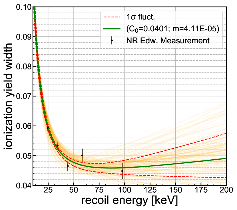
Figure 3: (Color online) Our fit to the nuclear-recoil ionization width using the MCMC procedure. The solid curve is the maximum-likelihood fit to the $C$ function, and the dashed lines are the assessed 1$\sigma$ statistical uncertainty bounds. The data points are the EDELWEISS Martineau et al. (2004) measured values for detector GGA3 and the transparent curves are a sampling of 100 realizations of $C(E_{r})$ using parameters pulled from the posterior parameter distributions.

The nuclear-recoil band width is well-reproduced by using the fitted $C(E_{r})$ added in quadrature to the base-level estimate. The base-level estimate is given in the Appendix and is symbolically referred to as $\sigma^{\mathrm{SAI}}_{\mathrm{NR}}$. Given the flexibility of our exact model for the ionization yield distribution, we proceeded to use this $C(E_{r})$ and its associated error to obtain the variance on $N$ as a function of recoil energy, parameterized by the intrinsic nuclear recoil Fano factor, $F_{\mathrm{nr}}$.

V Multiple scattering correction

For the EDELWEISS data the nuclear-recoil ionization yield information is generated via scattering of neutrons from a ²⁵²Cf source. Because of the use of neutrons, multiple scattering is an obvious effect that will increase the measured ionization yield width. The EDELWEISS study Martineau et al. (2004) accounted for this effect using a Monte Carlo simulation and concluded:

Although multiple interactions tend to lower $\langle Q\rangle$; this effect remains weak, and the $Q$ distribution associated with single interactions events is only slightly narrower and completely included in the wider band.

the “wider band” being the band that encompasses the measured nuclear recoils. In other words multiple scattering can not account for the full observed ionization yield width.

We have re-simulated the effect of multiple scattering in a detector that matches the EDELWEISS GGA3 germanium detector (approx. cylindrical with a 70 mm diameter and 20 mm thick). For this we have used a Geant4 Allison et al. (2006); Agostinelli et al. (2003) simulation where the geometry–aside from the germanium detector–was not made identical to the EDELWEISS setup, but where generic elements like typical cryostat materials and polyethylene shielding were included. Our specific geometry (from inside to outside) included: the germanium detector; an electronics “tower” made mostly of copper with small amounts of insulating carbon; an “inner vacuum chamber” wall made of stainless steel; liquid helium; a stainless steel Dewar with vacuum jacket; and a rectangular polyethylene shield and supporting structure (aluminum). The source is located between the Dewar and polyethylene shield, 66 cm below the detector at a radial distance of 35 cm from the cylindrical axis of the Dewar and germanium detector.

Our simulation uses Geant 4.10.1.p02 and the so-called “Shielding” physics list Agostinelli et al. (a). The main attribute of this physics list in the context of our analysis is the high-precision neutron-scattering library for neutron energies below 20 MeV. The use of this “NeutronHP” library Agostinelli et al. (b); Thulliez et al. (2022) gives more precise realizations of the nuclear recoils because of the implementation of the detailed low-energy neutron interaction library G4NDL. A small drawback of the library is that it sacrifices strict energy-momentum conservation on an event-by-event basis, but that is not an important deterrent for this study since the recoil spectrum is more correct.

While the simulation setup does not match the EDELWEISS geometry, we point out that the geometry will principally affect the energy distribution of the neutron flux near the detector. The yield width is insensitive to that distribution because all of our scattering neutrons lie above 20 keV, where the elastic scattering cross section is away from the resonance region, relatively flat, and well known Iwamoto, Osamu et al. (2020). Therefore, the distribution of multiple scatters within the detector–which does affect the $Q$ distribution–will not depend strongly on the energy distribution of the neutron flux or the geometry, but rather if the germanium elastic cross sections used are close to reality. The elastic cross sections used in our version of “NeutronHP” are in an energy region that has been well measured and match other evaluations like the JENDL 5.0 evaluation Iwamoto, Osamu et al. (2020).

We use this simulated data by applying the ionization yield model used in Sec. III. More precisely, we “tune” the sensor resolutions in the same way as produced the best match to the electron-recoil band width, take the ionization yield to be $\bar{Q}=0.16E_{r}^{0.18}$, and take the intrinsic nuclear recoil Fano factor to be zero.

The simulated ionization yield distributions in Fig. 4 show that the single scatter contribution has a clearly higher average yield than the distribution that includes all scatters. However, the width of the distribution is only modestly wider over the energy range shown (20–30 keV). The empirical distribution (Fig. 4 black dashed histogram) is clearly significantly wider than our simulation with multiple scatters included–a feature that gets more significant with increasing energy.

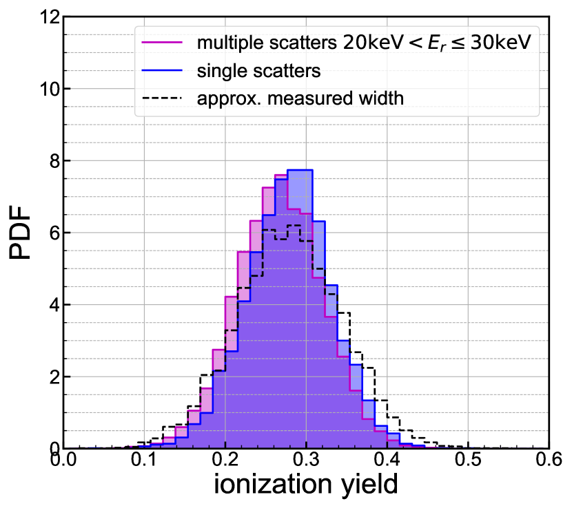
Figure 4: (Color online) Simulated ionization yield histograms of the single-scatter distribution (blue) and all-scatter distribution (magenta) for the energy range 20–30 keV. The black dashed histogram are single scatters with an “extra” resolution applied to bring the width of the distribution in line with what was measured by EDELWEISS as discussed in their publication Martineau et al. (2004).

We have systematically fit the distribution widths from the simulation as a function of energy and compared them with the single-scatter width predictions discussed previously. Figure 5 shows the ionization widths that result for a full simulated ²⁵²Cf data set with multiple scattering included. Of course, the resulting ionization widths are larger than would result from a nuclear recoil sample consisting only of single scatters. Since our ionization yield model only makes predictions for single scatters we compare the multiple scatters to that prediction to see how much wider the ionization yield distribution becomes. As in the previous section we fit a function $C_{m}(E_{r})=C_{0m}+m_{m}E_{r}$ that describes the quadrature addition necessary to bring the single-scatter prediction in line with the simulated multiple-scatter results. In this case we do not let $A$, $B$, $a_{H}$, or $\eta$ vary but set them equal to their best fit values from the MCMC in Sec. IV. The varying fit parameters are $C_{0m}$ and $m_{m}$.

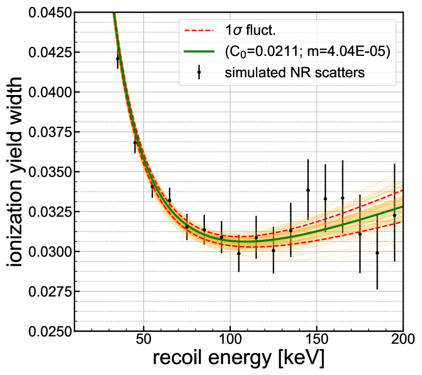
Figure 5: (Color online) A fit to the simulated multiple-scatter ionization width using the Geant4 recoil data, and our yield model. The points are the ionization yield widths of the simulated data, the solid line is the maximum likelihood fit to the $C_{m}$ function. The dashed lines are the assessed 1$\sigma$ statistical uncertainty bounds. The transparent curves are a sampling of 100 realizations of $C_{m}(E_{r})$ using parameters pulled from the posterior parameter distributions.

It is clear from the fit displayed in Fig. 5 that the quadrature addition needed to describe the effect of multiple scattering is observable but significantly less than what is required to describe the EDELWEISS ionization yield width data. This multiple-scatter correction to the yield widths will be used in Sec. VI to extract the required additional correction needed to describe the EDELWEISS data. We argue that this additional correction is related to unaccounted uncertainty in the fundamental ionization production by nuclear recoils; and can be described by an intrinsic nuclear recoil Fano factor.

VI Extracting the germanium intrinsic Fano factor

We posit that the reason the measured ionization variance on EDELWEISS’ GGA3 detector is larger than the expected when including multiple scattering (see Sec. V) is an unaccounted intrinsic ionization variance in the nuclear scattering process. We quantify this additional variance, by taking the quadrature subtraction of the corrections extracted in Secs. III and V. The result is a correction, $C^{\prime}(E_{r})$, that is equal to the intrinsic ionization variance. Equation 6 shows the relationship of the intrinsic variance to the previous corrections.

$$C^{\prime}(E_{r})=\sqrt{C(E_{r})^{2}-C_{m}(E_{r})^{2}}$$ (6)

Our intrinsic ionization variance is then converted into a Fano factor for nuclear recoils, $F_{\mathrm{nr}}$, as advocated in Sec. II. The conversion to the nuclear recoil Fano factor is made by assuming the intrinsic variance is produced by simply increasing the nuclear recoil Fano factor from $F_{\mathrm{nr}}$=0 to some finite (positive) value within the framework of the model given in Eq. 9 by setting the variance on the independent random variable $N$ taken to be $\sigma_{N}=\sqrt{F_{\mathrm{nr}}\bar{N}}$. The actual value of $F_{\mathrm{nr}}(E_{r})$ is then simply given by:

$$\sigma^{\mathrm{SAI}}_{\mathrm{NR}}(E_{r};F_{\mathrm{nr}})=\sqrt{C^{\prime}(E_{r})^{2}+\sigma^{\mathrm{SAI}}_{\mathrm{NR}}(E_{r};F_{\mathrm{nr}}=0)^{2}}$$ (7)

Figure 6 shows the extracted intrinsic Fano factor, $F_{\mathrm{nr}}$ , as a function of the recoil energy.

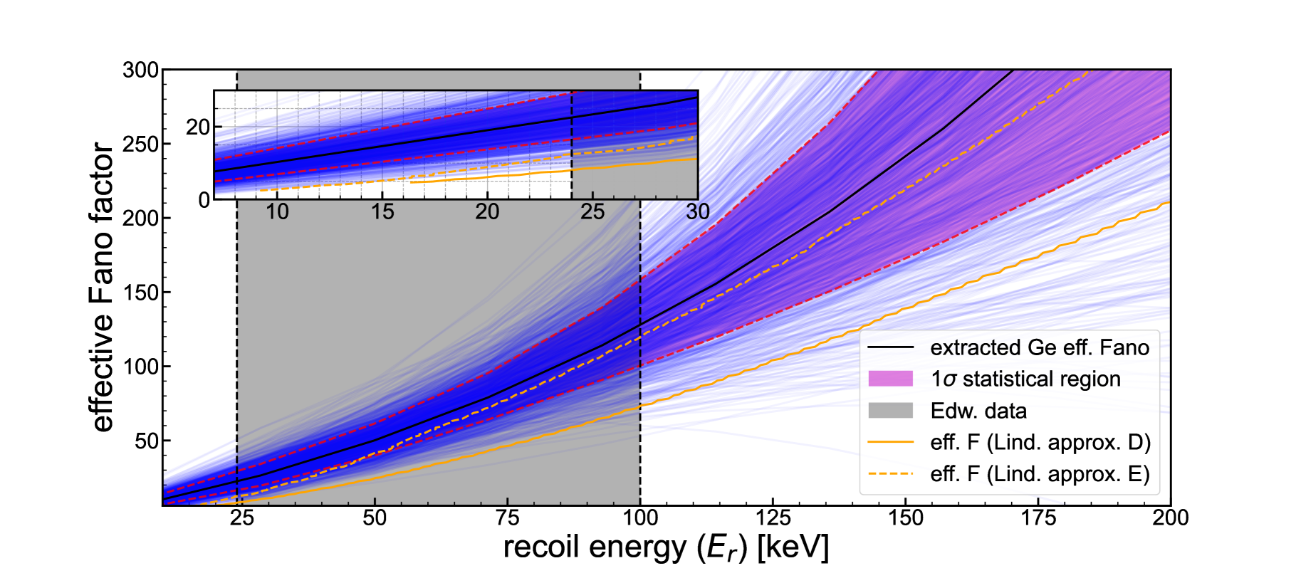
Figure 6: (Color online) The extracted nuclear-recoil intrinsic Fano factor for germanium using the EDELWEISS Martineau et al. (2004) data. The black line is the best fit, the magenta shaded region denotes the 1$\sigma$ statistical uncertainty region, and the inset shows a zoom of the region between 7 and 30 keV. The blue transparent curves are 1000 samples drawn from the MCMC posterior distribution–these give a sense for the presence of outlying behaviors. The gray shaded region is the region in which there are EDELWEISS yield width data; in that region the results are not an extrapolation. The Lindhard prediction for the nuclear recoil Fano factor are given in orange for the Approximations D (solid) and E (dashed). To produce those predictions we used a Lindhard model for the ionization yield with parameter $k$=0.157 Albakry et al. (2022).

The estimate for the uncertainties on the resulting $F_{\mathrm{nr}}(E_{r})$ were obtained from the MCMC posterior distribution of all of the parameters ($A$,$B$,$a_{H}$,$\eta$,$C_{0}$,$m$) in the original fit and the posterior distribution of the $C_{0m}$ and $m_{m}$ parameters in the multiples fit. A single realization of $F_{\mathrm{nr}}(E_{r})$ is obtained by using a sample of the original and multiples fit and then subtracting them in quadrature to get $C^{\prime}(E_{r})$. Each sample of $C^{\prime}$ is turned into a sample of $F_{\mathrm{nr}}$ through Eq. 7. The maximum likelihood parameters are taken as the central value for $F_{\mathrm{nr}}$ and we obtain the approximate 1$\sigma$ deviations by taking the standard deviation of all samples at each energy–these are plotted as the magenta band in Fig. 6.

These uncertainties include the systematic uncertainty on the result with contributions from several parameters which, while nominally fixed, are not known with certainty. They are, in order of decreasing importance: multiple scattering; a finite-binning uncertainty on the EDELWEISS ionization yield data; a possible departure of the quantity $V/\epsilon_{\gamma}$ from the nominal 4/3 value (fit parameter $\eta$); charge trapping (fit parameters $A$ and $B$); and the functional form of the average ionization yield. The uncertainties are obtained by directly estimating the contribution (in the case of the finite-binning) or including nuisance parameters in the 6-parameter MCMC Foreman-Mackey et al. (2013) fit to the EDELWEISS ionization yield width data for GGA3 for the extraction of $C(E_{r})$. For each of the parameters representing the systematic uncertainties, a prior was chosen that was reflective of the state of knowledge on the parameters.

Classification	Size (%)	Param.	Relevant Corr.
statistical (U)	40-80	$C_{0}$, $m$	none
multiple scattering (U)	$<$ 6	none	none
finite-binning (U)	5	-	-
$V/\epsilon_{\gamma}$ (U)	$<$ 20	$\eta$	$a_{H}$
charge trapping (U)	$<$ 20	$A$, $B$	$C_{0}$, $m$
yield variation (U)	$<$ 20	$A$, $B$	$C_{0}$, $m$
multiple scattering (C)	60-70	none	none

Table 2: The uncertainties and correction sizes for the extraction of the nuclear-recoil intrinsic Fano factor for germanium using the EDELWEISS Martineau et al. (2004) data. The first column lists uncertainties with a (U) and corrections with a (C). The third column are the parameters in the fit related to that category (if any). The last column lists the fit parameters that have relevant correlations with that particular category.

The total uncertainty is estimated in Figure 6 and the factional impact of each of the uncertainties or corrections are given in Tbl. 2.

VII Conclusions

We have espoused the preference for quantifying the inherent uncertainty on the number of electron-hole pairs produced as an intrinsic Fano factor, $F_{\mathrm{nr}}$, for nuclear recoils. We have also presented constraints on such a parameter from previous measurements on silicon and germanium–two important target materials for precision low-mass dark matter searches Agnese et al. (2017). In the latter case we extracted meaningful $F_{\mathrm{nr}}$ measurements by a technique that can be adapted to low-threshold detectors measuring ionization and heat, but that did not require a specialized neutron scattering setup. We have used the Lindhard predictions as a guide, with the hope that future experiments will be able to distinguish between approximations in that work and/or inspire the development of a more accurate framework.

Our results indicate that the intrinsic nuclear-recoil Fano factor is larger than expected for both silicon and germanium–24.3$\pm$0.2 and 26$\pm$8 respectively at 25 keV recoil energy. The expectation in some literature is based on the assumption that the number of phonons created is a Poisson random variable Mei et al. (2020). In that case the electron-recoil Fano factor is around 0.13 for germanium Alig et al. (1980) and the intrinsic nuclear-recoil Fano factor should be larger by about a factor of $1/\sqrt{\bar{Q}}$–still far lower than our suggested values. In the authors’ view, this would seem to indicate that for nuclear recoils the number of created phonons is not Poisson distributed and has a distribution that is significantly wider than naively expected; this wider distribution could then be imprinted on the electron-hole pairs in a way similar to the derivation in Mei et al. (2020). The authors do not see any reason why the number of phonons produced should have a Poisson distribution, in fact the Lindhard references explicitly compute an ionization variance that are out of line with that assumption Lindhard et al. (1963a). The Lindhard predictions for the intrinsic nuclear-recoil Fano factor are shown in Fig. 6 for germanium and have an $F_{\mathrm{nr}}$ at least as large as 8 at 25 keV recoil energy. Those intrinsic nuclear-recoil Fano predictions are not inconsistent with our measurement above around 50 keV but appear to be systematically lower than our measurement below 50 keV–perhaps due to an ionization yield that decreases more sharply toward lower recoil energy than the Lindhard theory suggests.

Based on our ionization yield model, which can describe EDELWEISS data well, the variance induced by the intrinsic Fano factor is correlated in its effect on ionization and heat resolutions. Roughly speaking, this means that the widening of “nuclear recoil bands” in low-threshold dark matter searches with discrimination capabilities (like SuperCDMS Agnese et al. (2014) and EDELWEISS Hehn et al. (2016)) may be smaller than one would naively expect.

There is a lot of existing data that might be exploited using our technique, but it is often true that precise resolution data is not published. If the sensor resolution is carefully extracted, then our technique might serve to extract $F_{\mathrm{nr}}$ more precisely for both silicon and germanium in the low-energy region. Such information is invaluable to low-mass nuclear-recoil dark matter searches in silicon and germanium that employ detectors without nuclear-recoil discrimination capabilities.

*

Appendix A Calculation of $\sigma_{\mathrm{NR}}$and cross-checks

A.1 Calculation of $\sigma_{\mathrm{NR}}$

Both the EDELWEISS and SuperCDMS detectors can be correctly modeled by assuming the measurements of the ionization and heat depend on three (approximately) independent random variables: the number of electron-hole pairs created in a detectable interaction, $N$; the variation (noise fluctuations) in the ionization sensor, $\delta I$; and the variation in the heat detection $\delta H$. The distributions of $\delta I$ and $\delta H$ have zero mean and are approximately normally distributed with an energy-dependent standard deviation given by the ionization and heat sensor resolutions. The typical measured quantities in these experiments are specific combinations of those random variables defined thusly:

$$\tilde{E}_{r} \equiv E_{r}+\left(1+\frac{V}{\epsilon_{\gamma}}\right)\delta H-\frac{V}{\epsilon_{\gamma}}\delta I$$ (8)

$$Q \equiv\frac{\epsilon_{\gamma}N+\delta I}{\tilde{E}_{r}}.$$

The variable $\tilde{E}_{r}$ is the measured recoil energy, $Q$ is the measured ionization efficiency (yield), $E_{r}$ is the true recoil energy, and $V$ is the voltage across the cylindrical detector. With this model, if the sensor resolutions are published (or otherwise known), the only remaining things needed to predict exact distributions for all the measured quantities are the true recoil energy distribution (which can be simulated) and the distribution of the random variable $N$. The latter is directly related to the Fano factor or the intrinsic nuclear-recoil Fano factor. Since $N$ is rather high for recoil energies above $\sim$10 keV the distribution is taken to be approximately normal, with the mean given by the average ionization yield at the particular recoil energy ($\bar{Q}(E_{r})$) and the width being given by the intrinsic Fano factor, $F_{\mathrm{nr}}$.

We have done the exact calculation simply by recognizing the joint conditional probability distribution for $\tilde{E}_{r}$ and $Q$ must have the following form:

$$P(Q,\tilde{E}_{r}|\delta H,\delta I,N,E_{r}) =\delta\left(\tilde{E}_{r}-\left[E_{r}+\left(1+\frac{V}{\epsilon_{\gamma}}\right)\delta H-\left(\frac{V}{\epsilon_{\gamma}}\right)\delta I\right]\right)$$ (9)

$$\times\delta\left(Q-\left[\frac{\epsilon_{\gamma}N+\delta I}{E_{r}+\left(1+V/\epsilon_{\gamma}\right)\delta H-(V/\epsilon_{\gamma})\delta I}\right]\right).$$

Equation 9 will correctly give the ionization yield ($Q$) distribution at a single measured energy or over a range of measured energies. The distribution close to normal for a wide range of parameters but not exactly normal. The distribution is especially far from normal when the heat or ionization have a large enough variance so that the measured recoil energy becomes consistent with zero. The ionization yield standard deviation with this ”exact” calculation is referred to as $\sigma_{\mathrm{NR}}$.

The procedure outlined above involves integrals that are difficult to accomplish analytically. For that reason, slower numerical techniques are used and the computation time makes it difficult to use (around 1 min for one calculation at one energy and parameter-value point). In this work, as discussed in Sections III,V, and VI, the fitting requires many evaluations of the function and so it must be approximated.

Part of the problem is not only the functional dependence on $E_{r}$, but the functional dependence on our nuisance parameters $A$, $B$, $a_{H}$, and $\eta$. In the general case–nuclear recoils with average yield modeled by the $A$ and $B$ parameters–we compute the “moment” expansion of $Q$ in Eq. 8 to order $1/E_{r}^{6}$. We refer to this expression as $\sigma^{\mathrm{SA}}_{\mathrm{NR}}$. For electron recoils, the agreement is quite good if we simply take this expansion with $A$=1 and $B$=0 (see Fig. 2). The expansion to lower order ($1/E_{r}^{2}$) is the expression used by EDELWEISS–$\sigma^{\mathrm{EDW}}_{\mathrm{NR}}$(see Eq. 3).

For nuclear recoils, the agreement is not as good, so we add a correction based on the preferred values of the nuisance parameters from our fit to the EDELWEISS data. Taking $A_{0}$=0.149, $B_{0}$=0.178, $a_{H0}$=0.038, and $\eta_{0}$=1.000 we can use the exact function to create a static correction to for use in the nuclear recoil case. This is the approximation we use to describe our nuclear recoil ionization yield widths in our fitting procedure of Sec. IV:

$$\sigma^{\mathrm{SAI}}_{\mathrm{NR}}(E_{r},A,B,\eta,F_{\mathrm{nr}}=0)^{2} =\sigma^{\mathrm{SA}}_{\mathrm{NR}}(E_{r},A,B,\eta,F_{\mathrm{nr}}=0)^{2}$$ (10)

$$+\left[\sigma_{\mathrm{NR}}(E_{r},A_{0},B_{0},\eta_{0},F_{\mathrm{nr}}=0)^{2}-\sigma^{\mathrm{SA}}_{\mathrm{NR}}(E_{r},A_{0},B_{0},\eta_{0},F_{\mathrm{nr}}=0)^{2}\right].$$

The form shown in Eq. 10 is much faster to compute than the exact version, but gives ionization yield widths which differ from the exact model by at most 7% over our parameter space ($E_{r}$ plus nuisance parameters).

A.2 Cross check with electron recoil Fano factor

One excellent check for consistency of our method is to fit the electron recoil ionization yield band and extract the electron recoil Fano factor, F. We cannot accomplish this with the real EDELWEISS data Martineau et al. (2004) that we’ve used for the majority of this paper because the data is not precise enough (about 10% relative uncertainty) and the Fano contribution to the ionization yield variance is expected only to be around 0.1%. This is in contrast to the nuclear recoil Fano contribution which we have measured to be at least 10%.

Instead what we’ve done is simulate electron recoil band data in a similar way as was done in Fig. 2, the high-precision simulated data points. We selected a Fano factor of F=0.15, adjusted the instrumental resolution so that the Fano contribution was about 1% in yield variance, and simulated the data with about 0.5% relative uncertainty on each data point. With this fit–using the same MCMC fitting method we used for nuclear recoils in this work–we extracted a Fano factor of F=0.13$\pm$0.08, consistent with the Fano factor we set for the simulation (F=0.15).

References

- Arnaud et al. (2018) Q. Arnaud et al., Astroparticle Physics 97, 54 (2018).
- Abdelhameed et al. (2019) A. H. Abdelhameed et al. (CRESST Collaboration), Phys. Rev. D 100, 102002 (2019).
- Angloher et al. (2014) G. Angloher et al., The European Physical Journal C 74, 3184 (2014).
- Aprile et al. (2018) E. Aprile et al. (XENON Collaboration 7), Phys. Rev. Lett. 121, 111302 (2018).
- Agnese et al. (2018) R. Agnese et al. (SuperCDMS Collaboration), Phys. Rev. Lett. 120, 061802 (2018).
- Lindhard et al. (1963a) J. Lindhard, V. Nielsen, M. Scharff, and P. Thomsen, Integral Equations Governing Radiation Effects. (NOTES ON ATOMIC COLLISIONS, III), Vol. 33 (Copenhagen, Denmark, 1963) pp. 1–42.
- Armengaud et al. (2019) E. Armengaud et al. (EDELWEISS Collaboration), Phys. Rev. D 99, 082003 (2019).
- Agnese et al. (2015) R. Agnese et al. (SuperCDMS Collaboration), Phys. Rev. D 92, 072003 (2015).
- Agnese et al. (2019) R. Agnese et al. (SuperCDMS Collaboration), Phys. Rev. D 99, 062001 (2019).
- Aguilar-Arevalo et al. (2020) A. Aguilar-Arevalo et al. (DAMIC Collaboration), Phys. Rev. Lett. 125, 241803 (2020).
- Tiffenberg et al. (2017) J. Tiffenberg et al., Phys. Rev. Lett. 119, 131802 (2017).
- Romani et al. (2018) R. K. Romani et al., Applied Physics Letters 112, 043501 (2018), https://doi.org/10.1063/1.5010699 .
- Villano et al. (2022) A. N. Villano et al., Phys. Rev. D 105, 083014 (2022).
- Scholz et al. (2016) B. J. Scholz, A. E. Chavarria, J. I. Collar, P. Privitera, and A. E. Robinson, Phys. Rev. D 94, 122003 (2016).
- Chavarria et al. (2016) A. E. Chavarria et al., Phys. Rev. D 94, 082007 (2016).
- Sorensen (2015) P. Sorensen, Phys. Rev. D 91, 083509 (2015).
- Dougherty (1992) B. L. Dougherty, Phys. Rev. A 45, 2104 (1992).
- Gerbier et al. (1990) G. Gerbier et al., Phys. Rev. D 42, 3211 (1990).
- Martineau et al. (2004) O. Martineau et al., Nuclear Instruments and Methods in Physics Research Section A: Accelerators, Spectrometers, Detectors and Associated Equipment 530, 426 (2004).
- Agnese et al. (2014) R. Agnese et al. (SuperCDMS Collaboration), Phys. Rev. Lett. 112, 241302 (2014).
- Bousselham et al. (2010) A. Bousselham, H. H. Barrett, V. Bora, and K. Shah, Nuclear Instruments and Methods in Physics Research Section A: Accelerators, Spectrometers, Detectors and Associated Equipment 620, 359 (2010).
- Mei et al. (2020) D.-M. Mei et al., Journal of Physics G: Nuclear and Particle Physics 47, 105106 (2020).
- Fano (1946) U. Fano, Phys. Rev. 70, 44 (1946).
- Note (1) Note that the convenience is in comparison to the electron recoil case and the qualitative similarity to the Poisson distribution, the underlying causes of the variance are different in the nuclear recoil case, arising from the inherent randomness in the energy deposition process in terms of the fraction of energy given to the lattice. The electron recoils have approximately zero energy given to the lattice.
- Note (2) The measurement temperatures are different for these measurements, being 90 K, 77 K, and 87 K for the lowest-to-highest measurements.
- Yamaya et al. (1979) T. Yamaya, R. Asano, H. Endo, and K. Umeda, Nuclear Instruments and Methods 159, 181 (1979).
- Eberhardt (1970) J. Eberhardt, Nuclear Instruments and Methods 80, 291 (1970).
- Palms et al. (1969) J. Palms, P. Venugopala Rao, and R. Wood, Nuclear Instruments and Methods 76, 59 (1969).
- Perotti and Fiorini (1999) F. Perotti and C. Fiorini, Nuclear Instruments and Methods in Physics Research Section A: Accelerators, Spectrometers, Detectors and Associated Equipment 423, 356 (1999).
- Zulliger and Aitken (1970) H. R. Zulliger and D. W. Aitken, IEEE Transactions on Nuclear Science 17, 187 (1970).
- Lindhard et al. (1968) J. Lindhard, V. Nielsen, and M. Scharff, Approximation Method in Classical Scattering by Screened Coulomb Fields (NOTES ON ATOMIC COLLISIONS, I), Matematisk-fysiske meddelelser (Copenhagen, Denmark, 1968) pp. 3–32.
- Lindhard et al. (1963b) J. Lindhard, M. Scharff, and H. Schioett, Range Concepts and Heavy Ion Ranges (NOTES ON ATOMIC COLLISIONS, II), Kgl. Danske Videnskab. Selskab. Mat. Fys. Medd., Vol. 33 (Copenhagen, Denmark, 1963) pp. 1–38.
- Lindhard and Scharff (1961) J. Lindhard and M. Scharff, Phys. Rev. 124, 128 (1961).
- Kennedy (2017) A. Kennedy, SuperCDMS Prototype Detector Design and Testing, Ph.D. thesis, University of Minnesota (2017).
- Note (3) Actually because of the definition of quenching as the expected width on this quantity needs to be derived more carefully than the standard .
- Note (4) As noted before the electron recoils also have a Fano factor but its effect was included in the measurement of the EDELWEISS resolution parameters.
- Note (5) Eq. 4 has the same form when written in terms of the instrumental FWHM values, except that the constants will have to be multiplied by a factor, due to convention is reported as if this equation is the FWHM version.
- Foreman-Mackey et al. (2013) D. Foreman-Mackey, D. W. Hogg, D. Lang, and J. Goodman, Publications of the Astronomical Society of the Pacific 125, 306 (2013).
- Villano and Roberts (2022) A. N. Villano and A. Roberts, “Intrinsic fano factor of nuclear recoils for dark matter searches,” (2022).
- Allison et al. (2006) J. Allison et al., IEEE Transactions on Nuclear Science 53, 270 (2006).
- Agostinelli et al. (2003) S. Agostinelli et al., Nuclear Instruments and Methods in Physics Research Section A: Accelerators, Spectrometers, Detectors and Associated Equipment 506, 250 (2003).
- Agostinelli et al. (a) S. Agostinelli et al., Geant4 Guide for Physics Lists, Geant4 Collaboration (a).
- Agostinelli et al. (b) S. Agostinelli et al., Geant4 Physics Reference Manual, Chapter 39: Low Energy Neutron Interactions, Geant4 Collaboration (b).
- Thulliez et al. (2022) L. Thulliez, C. Jouanne, and E. Dumonteil, Nuclear Instruments and Methods in Physics Research Section A: Accelerators, Spectrometers, Detectors and Associated Equipment 1027, 166187 (2022).
- Iwamoto, Osamu et al. (2020) Iwamoto, Osamu et al., EPJ Web Conf. 239, 09002 (2020).
- Albakry et al. (2022) M. F. Albakry et al., Phys. Rev. D 105, 122002 (2022).
- Agnese et al. (2017) R. Agnese et al. (SuperCDMS Collaboration), Phys. Rev. D 95, 082002 (2017).
- Alig et al. (1980) R. C. Alig, S. Bloom, and C. W. Struck, Phys. Rev. B 22, 5565 (1980).
- Hehn et al. (2016) L. Hehn et al., The European Physical Journal C 76, 548 (2016).