Nonparametric, Nonasymptotic Confidence Bands with
Paley-Wiener Kernels for Band-Limited Functions

Abstract

The paper introduces a method to construct confidence bands for bounded, band-limited functions based on a finite sample of input-output pairs. The approach is distribution-free w.r.t. the observation noises and only the knowledge of the input distribution is assumed. It is nonparametric, that is, it does not require a parametric model of the regression function and the regions have non-asymptotic guarantees. The algorithm is based on the theory of Paley-Wiener reproducing kernel Hilbert spaces. The paper first studies the fully observable variant, when there are no noises on the observations and only the inputs are random; then it generalizes the ideas to the noisy case using gradient-perturbation methods. Finally, numerical experiments demonstrating both cases are presented.

statistical learning, stochastic systems, estimation, nonlinear system identification

1 Introduction

Regression is one of the fundamental problems of statistics, system identification, signal processing and machine learning [1]. Given a finite sample of input-output pairs, the typical aim is to estimate the so-called regression function, which, given an input, encodes the conditional expectation of the corresponding output [2]. There are several well-known (parametric and nonparametric) approaches for regression, from linear regression to neural networks and kernel methods, which provide point-estimates from a given model class [3].

However, sole point-estimates are often not sufficient and region-estimates are also needed, for example, to support robust approaches. These region-estimates have several variants, such as confidence regions for the “true” function generating the observations [4]; for the expected output at a given input [5]; and prediction regions for the next (noisy) observation [6].

In this paper, we focus on building confidence bands for the regression function. These bands have natural connections to filtering and smoothing methods. While in a parametric setting such region-estimates are typically induced by confidence sets in the parameter space, in a nonparametric setting this indirect approach is not feasible. Therefore, nonparametic confidence bands for the expected outputs should be constructed directly.

Regarding prediction intervals for the next observation, promising distribution-free approaches are interval predictor models (IPMs) based on the scenario approach [7, 8], and the conformal prediction framework also offers several nonparametric methods for regression and classification [6].

If the data is jointly Gaussian, a powerful methodology is offered by Gaussian process regression [5] that can provide prediction regions for the outputs, and credible regions for the expected outputs. However, the Gaussianity assumption is sometimes unrealistic that calls for alternative approaches.

In this paper, we suggest a nonparametric approach using Paley-Wiener kernels, to build data-driven simultaneous confidence bands for an unknown bounded, band-limited function, based on an independent and identically distributed (i.i.d.) sample of input-output pairs. The method is distribution-free in the sense that only very mild assumptions are needed about the observation noises, such as they are distributed symmetrically about zero. On the other hand, we assume that the distribution of the inputs is known, particularly, we assume uniformly distributed inputs, as more general cases can often be traced back to this assumption. First, the case without observation noises is studied, then the ideas are extended to the general, noisy case. The results are supported by both non-asymptotic theoretical guarantees and numerical experiments.

2 Kernels and Band-Limited Functions

Kernel methods have an immerse range of applications in machine learning and related fields [9]. In this section, we review some of their fundamental theoretical concepts.

2.1 Reproducing Kernel Hilbert Spaces

A Hilbert space $\mathcal{H}$ of $f:\mathbb{X}\to\mathbb{R}$ functions with an inner product $\langle\cdot,\cdot\rangle_{\mathcal{H}}$ is called a Reproducing Kernel Hilbert Space (RKHS), if each Dirac functional, which evaluates functions at a point, $\delta_{z}:f\to f(z)$, is bounded for all $z\in\mathbb{X}$, that is $\forall z\in\mathbb{X}:\exists\,\kappa_{z}>0$ with $|\hskip 0.85358pt\delta_{z}(f)\hskip 0.85358pt|\leq\kappa_{z}\,\|f\|_{\mathcal{H}}$ for all $f\in\mathcal{H}$.

Then, by building on the Riesz representation theorem, a unique kernel, $k:\mathbb{X}\times\mathbb{X}\to\mathbb{R}$, can be constructed encoding the Dirac functionals satisfying $\langle k(\cdot,z),f\rangle_{\mathcal{H}}=f(z),$ for all $z\in\mathbb{X}$ and $f\in\mathcal{H}$, which formula is called the reproducing property. As a special case of this property, we also have for all $z,s\in\mathbb{X}$ that $k(z,s)=\langle k(\cdot,z),k(\cdot,s)\rangle_{\mathcal{H}}.$ Therefore, the kernel of an RKHS is a symmetric and positive-definite function.

Furthermore, the Moore-Aronszajn theorem asserts that the converse statement holds true, as well: for every symmetric and positive-definite function $k:\mathbb{X}\times\mathbb{X}\to\mathbb{R}$, there exists a unique RKHS for which $k$ is its reproducing kernel [10].

The Gram or kernel matrix of a given kernel $k$ w.r.t. (input) points $x_{1},\dots,x_{n}$ is $K_{i,j}\doteq k(x_{i},x_{j})$, for all $i,j\in[n]\doteq\{1,\dots,n\}$. Observe that $K\in\mathbb{R}^{n\times n}$ is always positive semi-definite. A kernel is called strictly positive-definite, if its Gram matrix is positive-definite for all distinct inputs $\{x_{i}\}$.

Archetypal kernels include the Gaussian kernel $k(z,s)=\exp(-||z-s||^{2}/(2\sigma^{2})),$ where $\sigma>0$; the polynomial kernel $k(z,s)=(\langle z,s\rangle+c)^{p},$ where $c\geq 0$, $p\in\mathbb{N}$; and the sigmoidal kernel $k(z,s)=\tanh(a\langle z,s\rangle+b),$ for some $a,b\geq 0$.

2.2 Paley-Wiener Spaces

Let $\mathcal{H}$ be the space of $f\in\mathcal{L}^{2}(\mathbb{R},\lambda)$ functions, where $\lambda$ is the Lebesgue measure, such that the support of the Fourier transform of $f$ is included in $[\hskip 0.85358pt-\eta,\,\eta\hskip 1.42262pt]$, where $\eta>0$. It is a subspace of $\mathcal{L}^{2}$ and thus we use the $\mathcal{L}^{2}$ inner product:

$$\langle f,g\rangle_{\mathcal{H}}\,\doteq\int_{\mathbb{R}}f(x)\,g(x)\>\mathrm{d}\lambda(x).$$

This space of band-limited functions, called the Paley-Wiener space [10], is an RKHS. Its reproducing kernel is

$$k(z,s)\,\doteq\,\frac{\sin(\eta(z-s))}{\pi(z-s)},$$

for $z\neq s$, where $z,s\in\mathbb{R}$; and $k(z,z)\doteq\eta/\pi$. Henceforth, we will work with the above defined Paley-Wiener kernel.

Remark 1

Paley-Wiener spaces can also be defined on $\mathbb{R}^{d}$ [11], but for simplicity we focus on the scalar input case.

3 Nonparametric Confidence Bands

Let $(x_{1},y_{1}),\dots,(x_{n},y_{n})$ be a finite sample of i.i.d. pairs of random variables with unknown joint distribution $\mathbb{P}_{\!\scriptscriptstyle X,Y}$, where $x_{k}$ and $y_{k}$ are $\mathbb{R}$-valued, and $\mathbb{E}[\hskip 0.85358pty^{2}_{k}\hskip 0.85358pt]<\infty$. We assume that

$$y_{k}\,=\,f_{*}(x_{k})+\varepsilon_{k},$$

for $k\in[n]$, where $\mathbb{E}[\hskip 0.85358pt\varepsilon_{k}\hskip 0.85358pt]=0$. Variables $\{\varepsilon_{k}\}$ represent the measurement or observation noises on the “true” $f_{*}$.

We call $f_{*}$ the regression function [1], as on the support of $\{x_{k}\}$ it can also be written as $f_{*}(x)\,=\,\mathbb{E}\left[\hskip 1.42262ptY\hskip 1.42262pt|\hskip 1.42262ptX=x\hskip 1.42262pt\right]$, where $(X,Y)$ is a random vector with distribution $\mathbb{P}_{\!\scriptscriptstyle X,Y}$.

3.1 Objectives and Reliability

Our aim is to build a (simultaneous) confidence band for $f_{*}$, i.e., a function $I:\mathcal{D}\to{\mathbb{R}\times\mathbb{R}}$, where $\mathcal{D}$ is the support of the input distribution, such that $I(x)=(\hskip 0.85358ptI_{1}(x),I_{2}(x)\hskip 0.85358pt)$ specifies the endpoints of an interval estimate for $f_{*}(x)$, for all $x\in\mathcal{D}$. More precisely, we would like to construct $I$ with

$$\nu(I)\,\doteq\,\mathbb{P}\big{(}\,\forall x\in\mathcal{D}:{I_{1}(x)\leq f_{*}(x)\leq I_{2}(x)}\,\big{)}\,\geq\,1-\alpha,$$

where $\alpha\in(0,1)$ is a user-chosen risk probability, and $\nu(I)$ is the reliability of the confidence band. Let us introduce

$$\mathcal{I}\,\doteq\,\big{\{}\hskip 1.42262pt(x,y)\in\mathcal{D}\times\mathbb{R}:y\in[\hskip 0.85358ptI_{1}(x),I_{2}(x)\hskip 0.85358pt]\hskip 1.42262pt\big{\}}.$$

Based on this, the reliability is $\nu(I)=\mathbb{P}(\,\mathrm{graph}_{\mathcal{D}}(f_{*})\subseteq\mathcal{I}\,)$, where we define $\mathrm{graph}_{\mathcal{D}}(f_{*})\doteq\{\,(x,f_{*}(x)):x\in\mathcal{D}\,\}$.

For notational simplicity, we will use $I(x)=\emptyset$ to denote $I(x)=(\hskip 0.85358pt1,-1\hskip 0.85358pt)$, i.e., the endpoints of an empty interval.

Hence, we aim at building a confidence band that contains the graph (w.r.t. domain $\mathcal{D}$) of the “true” $f_{*}$ with a user-chosen probability level. Moreover, we would like to have a distribution-free method (w.r.t. the noises) and the region should have finite-sample guarantees without a parametric model of $f_{*}$, namely, we take a nonparametric approach.

Remark 2

We note here, as well, that in the IPMs [7][8] and in the conformal prediction framework [6], the aim is to build a guaranteed prediction region for the next observation, while here we aim at predicting the value of the regression function instead. In this sense, our objective is similar to that of the region estimates of Gaussian process regression [5], however, without the assumption of joint Gaussianity.

3.2 Main Assumptions

Our core assumptions can be summarized as follows:

A​​ 0

The dataset, $(x_{1},y_{1}),\dots,(x_{n},y_{n})\in\mathbb{R}\times\mathbb{R}$, is an i.i.d. sample of input-output pairs; and $\mathbb{E}[\hskip 0.85358pty^{2}_{k}\hskip 0.85358pt]<\infty$, for $k\in[n]$.

A​​ 1

Each (measurement) noise, $\varepsilon_{k}\doteq y_{k}-f_{*}(x_{k})$, for $k\in[n]$, has a symmetric probability distribution about zero.

A​​ 2

The inputs, $\{x_{k}\}$, are distributed uniformly on $[\hskip 1.13809pt0,1\hskip 0.56905pt]$.

A​​ 3

Function $f_{*}$ is from a Paley-Wiener space $\mathcal{H}$; $\forall\,x\in[\hskip 1.13809pt0,1\hskip 0.56905pt]:{|f_{*}(x)|}\leq 1$; and $f_{*}$ is almost time-limited to $[\hskip 1.13809pt0,1\hskip 0.85358pt]:$

$$\int_{\mathbb{R}}f^{2}_{*}(x)\,\mathbb{I}(x\notin[\hskip 1.13809pt0,1\hskip 0.56905pt])\>\mathrm{d}\lambda(x)\,\leq\,\delta_{0},$$

where $\mathbb{I}(\cdot)$ is an indicator and $\delta_{0}>0$ is a universal constant.

Now, let us briefly discuss these assumptions. The i.i.d. requirement of A ‣ 3.2 is standard in mathematical statistics and supervised learning [12]. The square-integrability of the outputs is needed to estimate the $\mathcal{L}^{2}$ norm of $f_{*}$ based on the sample and to have a well-defined regression function. The assumption on the noises, A1, is very mild, as most standard distributions (e.g., Gauss, Laplace and uniform) satisfy this.

Our strongest assumption is certainly A2, which basically amounts to the assumption that we know the distribution of the inputs and it is absolutely continuous. The more general case when the inputs, $\{x^{\prime}_{k}\}$, have a known, strictly monotone increasing and continuous cumulative distribution function $F$, could be traced back to assumption A2, since it is well-known that $x_{k}\doteq F(x^{\prime}_{k})$ is distributed uniformly on $[\hskip 1.13809pt0,1\hskip 0.56905pt]$.

Assumption A3, especially limiting the frequency domain of $f_{*}$, is needed to restrict the model class and to ensure that we can effectively generalize to unknown data points. We allow the “true” function to be defined outside the support of the inputs, cf. the Fourier uncertainty principle[13], but the part of $f_{*}$ outside of $\mathcal{D}=[\hskip 1.13809pt0,1\hskip 0.56905pt]$ should be “negligible”, i.e., its norm cannot exceed a (known) small constant, $\delta_{0}$.

A crucial property of Paley-Wiener spaces is that their norms coincide with the standard $\mathcal{L}^{2}$ norm, which will allow us to efficiently upper bound $\|f_{*}\|_{\mathcal{H}}^{2}$ based on the sample.

4 Confidence Bands: Noise-Free Case

In order to motivate our solution, we start with a simplified problem, in which we observe the regression function perfectly at random inputs. In this noise-free case, we can recall the celebrated Nyquist–Shannon sampling theorem, which states that a band-limited function can be fully reconstructed from the samples, assuming the sampling rate exceeds twice the maximum frequency. On the other hand, if we only have a small number of observations, we cannot apply this result. Nevertheless, we still would like to have at least a region estimate. In this section we provide such an algorithm.

Recall that for a dataset $\{(x_{k},y_{k})\}$, where inputs $\{x_{k}\}$ are distinct (which has probability one under A2), the element from $\mathcal{H}$ that has the minimum norm and interpolates each output $y_{k}$ at the corresponding input $x_{k}$, that is

$$\bar{f}\,\doteq\,\operatornamewithlimits{arg\,min}\big{\{}\,\|\hskip 0.85358ptf\hskip 1.13809pt\|_{\mathcal{H}}:f\in\mathcal{H}\hskip 4.2679pt\&\hskip 4.2679pt\forall\hskip 0.85358ptk\in[n]:f(x_{k})=\,y_{k}\,\big{\}},\vspace{-0.5mm}$$

takes the following form [10] for all input $x\in\mathbb{X}:$

$$\bar{f}(x)\,=\,\sum_{k=1}^{n}\bar{\alpha}_{k}k(x,x_{k}),\vspace{-0.5mm}$$

where the weights are $\bar{\alpha}=K^{-1}y$ with $y\doteq(y_{1},\dots,y_{n})^{\mathrm{T}}$ and $\bar{\alpha}\doteq(\bar{\alpha}_{1},\dots,\bar{\alpha}_{n})^{\mathrm{T}}$; we also used that the Paley-Wiener kernel is strictly positive-definite, thus matrix $K$ is invertible.

We will exploit, as well, that the norm square of $\bar{f}$ is

$$\|\hskip 0.85358pt\bar{f}\hskip 1.13809pt\|_{\mathcal{H}}^{2}=\bar{\alpha}^{\mathrm{T}}K\bar{\alpha},\vspace{-0.5mm}$$

which is a direct consequence of the reproducing property.

Assuming we have a stochastic upper bound for the norm square of the regression function, denoted by $\kappa$, the idea of our construction is as follows. We include those $(x_{0},y_{0})$ pairs in the confidence band, for which the minimum norm interpolation of $\{(x_{k},y_{k})\}\,\cup\,\{(x_{0},y_{0})\}$, namely, which simultaneously interpolates the original dataset and $(x_{0},y_{0})$, has a norm square which is less than or equal to $\kappa$. In order to make this approach practical, we need (1) a guaranteed upper bound for the norm square of the “true” data-generating function; and (2) an efficient method to decide the endpoints of the confidence interval for each potential input $x_{0}\in\mathcal{D}$.

4.1 Bounding the Norm: Noise-Free Case

It is easy to see that in the noise-free case, if $y_{k}=f_{*}(x_{k})$, for $k\in[n]$, the norm square of $f_{*}$ can be estimated by

$$\frac{1}{n}\sum_{k=1}^{n}y_{k}^{2}=\frac{1}{n}\sum_{k=1}^{n}f_{*}^{2}(x_{k})\approx\mathbb{E}\big{[}f^{2}_{*}(X)\big{]}\approx\|\hskip 0.85358ptf_{*}\hskip 1.13809pt\|_{2}^{2}=\|\hskip 0.85358ptf_{*}\hskip 1.13809pt\|_{\mathcal{H}}^{2},$$

since in the Paley-Wiener space the norm is the $\mathcal{L}^{2}$ norm, and we also used that $\{x_{k}\}$ are uniform on domain $\mathcal{D}=[\hskip 1.13809pt0,1\hskip 0.56905pt]$.

As the next lemma demonstrates, we can construct such a guaranteed upper bound using the Hoeffding inequality:

Lemma 1

Assuming A ‣ 3.2, A2, A3 and that $y_{k}=f_{*}(x_{k})$, for $k\in[n]$, we have for any risk probability $\alpha\in(0,1)$,

$$\mathbb{P}\big{(}\left\lVert f_{*}\right\rVert_{\mathcal{H}}^{2}\leq\kappa\hskip 0.85358pt\big{)}\,\geq\,1-\alpha,$$

with the following choice of the upper bound $\kappa$:

$$\kappa\,\doteq\,\frac{1}{n}\sum_{k=1}^{n}y_{k}^{2}+\sqrt{\frac{\ln(\alpha)}{-2n}}+\delta_{0}.$$

Proof 4.1.

By using the notation ${R}\doteq\nicefrac{{1}}{{n}}\sum_{k=1}^{n}y_{k}^{2}$, we have

$$\mathbb{E}[\hskip 0.85358pt{R}\hskip 0.85358pt]\,=\,\|\hskip 0.85358ptf_{*}\cdot\mathbb{I}_{\mathcal{D}}\hskip 0.85358pt\|_{2}^{2}\,\geq\,\|\hskip 0.85358ptf_{*}\hskip 1.13809pt\|_{\mathcal{H}}^{2}-\delta_{0},$$

where $\mathbb{I}_{\mathcal{D}}$ is the indicator function of $\mathcal{D}=[\hskip 1.13809pt0,1\hskip 0.56905pt]$. That is, ${R}$ is a Monte Carlo estimate of the integral of this $\mathcal{L}^{2}$ norm.

Then, from the Hoeffding inequality, for all $t>0$:

$$\mathbb{P}({R}-\mathbb{E}[\hskip 0.85358pt{R}\hskip 0.85358pt]\leq-t)\leq\mbox{exp}(-2nt^{2}).$$

According to the complement rule, we also have

$$\mathbb{P}(\mathbb{E}[\hskip 0.85358pt{R}\hskip 0.85358pt]<{R}+t)\geq 1-\mbox{exp}(-2nt^{2}).$$

We would like choose a threshold $t>0$ such that

$$1-\alpha\,\leq\,\mathbb{P}(\mathbb{E}[\hskip 0.85358pt{R}\hskip 0.85358pt]<{R}+t).$$

This inequality is satisfied if we choose a $t>0$ with

$$1-\alpha\leq 1-\mbox{exp}(-2nt^{2})\;\Longrightarrow\;\mbox{exp}(-2nt^{2})\leq\alpha.$$

After taking the natural logarithm, we get $-2nt^{2}\leq\ln(\alpha)$, hence, the choice of $t^{*}=\sqrt{\ln(\alpha)/(-2n)}$ guarantees

$$\mathbb{P}\big{(}\hskip 0.85358pt\|\hskip 0.85358ptf_{*}\hskip 1.13809pt\|_{\mathcal{H}}^{2}\geq{R}+t^{*}+\delta_{0}\hskip 0.85358pt\big{)}\leq\alpha,$$

which completes the proof of the lemma.

4.2 Interval Endpoints: Noise-Free Case

Now, we construct a confidence interval for a given input query point $x_{0}\in\mathcal{D}$, for which $x_{0}\neq x_{k}$, for $k\in[n]$. That is, we build an interval $[I_{1}(x_{0}),I_{2}(x_{0})]$ that contains $f_{*}(x_{0})$ with probability at least $1-\alpha$, where $\alpha\in(0,1)$ is given.

First, we extend the Gram matrix with query point $x_{0}$,

$$K_{0}({i+1},{j+1})\,\doteq\,k(x_{i},x_{j}),$$

for $i,j=0,1,\dots,n$. As $\{x_{k}\}_{k=0}^{n}$ are distinct (a.s.), this Gramian can be inverted. Hence, for any $y_{0}$, the minimum norm interpolation of $(x_{0},y_{0}),(x_{1},y_{1}),\dots,(x_{n},y_{n})$ is

$$\tilde{f}(x)\,=\,\sum_{k=0}^{n}\tilde{\alpha}_{k}k(x,x_{k}),$$

where the weights are $\tilde{\alpha}=K_{0}^{-1}\tilde{y}$ with $\tilde{y}\doteq(y_{0},y_{1},\dots,y_{n})^{\mathrm{T}}$ and $\tilde{\alpha}\doteq(\tilde{\alpha}_{0},\dots,\tilde{\alpha}_{n})^{\mathrm{T}}.$ The norm square of $\tilde{f}$ is

$$\|\hskip 0.85358pt\tilde{f}\hskip 1.13809pt\|_{\mathcal{H}}^{2}\,=\,\tilde{\alpha}^{\mathrm{T}}K_{0}\tilde{\alpha}\,=\,\tilde{y}^{\mathrm{T}}K_{0}^{-1}K_{0}K_{0}^{-1}\tilde{y}\,=\,\tilde{y}^{\mathrm{T}}K_{0}^{-1}\tilde{y}.$$

Since the output query point $y_{0}$ in $\tilde{y}=(y_{0},y^{\mathrm{T}})^{\mathrm{T}}$ is arbitrary, we can compute the minimum norm needed to interpolate the original dataset extended by $(x_{0},y_{0})$ for any candidate $y_{0}$.

Therefore, having a bound $\kappa$ on the norm square (which is guaranteed with probability $\geq 1-\alpha$), we can compute the highest and the lowest $y_{0}$ values which can be interpolated with a function from $\mathcal{H}$ having at most norm square $\kappa$.

This leads to the following two optimization problems:

$$\begin{split}\mbox{min\,/\,max}&\quad y_{0}\\[1.42262pt] \mbox{subject to}&\quad(y_{0},y^{\mathrm{T}})K_{0}^{-1}(y_{0},y^{\mathrm{T}})^{\mathrm{T}}\leq\,\kappa\\[2.84526pt] \end{split}$$ (1)

where “min / max” means that we have to solve the problem as a minimization and also as a maximization (separately).

The optimal values of these problems, denoted by $y_{\mathrm{min}}$ and $y_{\mathrm{max}}$, respectively, determine the endpoints of the confidence interval for $f_{*}(x_{0})$, that is $I_{1}(x_{0})\doteq y_{\mathrm{min}}$ and $I_{2}(x_{0})\doteq y_{\mathrm{max}}$.

Problems (1) are convex, moreover, as we will show, their optimal vales can be calculated analytically. First, note that the only decision variable of these problems is $y_{0}$, everything else is constant (including the input $x_{0}$, which is also given).

Let us partition the inverse Gramian, $K_{0}^{-1}$, as

$$\begin{bmatrix}\;c&b^{\mathrm{T}}\\ \;b&A\,\end{bmatrix}\doteq\,K_{0}^{-1}\!\!,$$

where $c\in\mathbb{R}$, $b\in\mathbb{R}^{n}$ and $A\in\mathbb{R}^{n\times n}$; after which

$$\quad(y_{0},y^{\mathrm{T}})K_{0}^{-1}(y_{0},y^{\mathrm{T}})^{\mathrm{T}}=\,c\,y_{0}^{2}+2\,b^{\mathrm{T}}y\,y_{0}+y^{\mathrm{T}}Ay.$$

Then, introducing $a_{0}\doteq c$, $b_{0}\doteq 2b^{\mathrm{T}}y$ and $c_{0}=y^{\mathrm{T}}Ay-\kappa$, the two optimization problems (1) can be written as

$$\begin{split}\mbox{min\,/\,max}&\quad y_{0}\\[1.42262pt] \mbox{subject to}&\quad a_{0}y_{0}^{2}+b_{0}y_{0}+c_{0}\,\leq\,0\end{split}$$ (2)

in which $a_{0}$, $b_{0}$ and $c_{0}$ are constants (w.r.t. the optimization).

Since these are (convex) quadratic programming problems (with linear objectives), their optimal solutions must be on the boundary of the constraint. This can be easily verified directly, for example, by the technique of Lagrange multipliers.

There are at most two solutions of the quadratic equation $a_{0}y_{0}^{2}+b_{0}y_{0}+c_{0}=0.$ The smaller one will be denoted by $y_{\mathrm{min}}$ and the larger one by $y_{\mathrm{max}}$ (they are allowed to be the same, if there is only one solution). Then, we set $I_{1}(x_{0})\doteq y_{\mathrm{min}}$, and $I_{2}(x_{0})\doteq y_{\mathrm{max}}$; or $I(x_{0})\doteq\emptyset$, in case there is no solution. Finally, we define $I_{1}(x_{k})=I_{2}(x_{k})=y_{k}$, for all $k\in[n]$, as the outputs are noise-free, that is $y_{k}=f_{*}(x_{k})$, for $k\in[n]$.

Table 1:

Pseudocode: Confidence interval for the noise-free case
Input:	Data sample $\{(x_{k},y_{k})\}_{k=1}^{n}$, input query point $x_{0}\in\mathcal{D}$,
	and risk probability $\alpha\in(0,1)$.
Output:	The endpoints of the confidence interval $[\hskip 0.85358ptI_{1}(x_{0}),I_{2}(x_{0})\hskip 0.85358pt]$
	which has confidence probability at least $1-\alpha$.
1.	If $x_{0}=x_{k}$ for any $k\in[n]$, return $I_{1}(x_{0})=I_{2}(x_{0})=y_{k}$.
2.	Calculate $\kappa\doteq\frac{1}{n}\sum_{k=1}^{n}y_{k}^{2}+\sqrt{\frac{\log(\alpha)}{-2n}}+\delta_{0}$.
3.	Create the extended Gram matrix
	$K_{0}(i+1,j+1)\doteq k(x_{i},x_{j}),$ for $i,j=0,1,...,n$.
4.	Calculate $K_{0}^{-1}$ and partition it as:
	$\begin{bmatrix}\;c&b^{\mathrm{T}}\\ \;b&A\,\end{bmatrix}\doteq\,K_{0}^{-1}$
5.	Solve the quadratic equation $a_{0}y_{0}^{2}+b_{0}y_{0}+c_{0}=0$,
	where $a_{0}\doteq c$, $b_{0}\doteq 2b^{\mathrm{T}}y$ and $c_{0}=y^{\mathrm{T}}Ay-\kappa$.
6.	If there is no solution, return $I(x_{0})\doteq\emptyset$; otherwise return
	$I_{1}(x_{0})\doteq y_{\mathrm{min}}$, and $I_{2}(x_{0})\doteq y_{\mathrm{max}}$, where $y_{\mathrm{min}}\leq y_{\mathrm{max}}$
	are the solutions (which are allowed to coincide).

Table 1 summarizes the proposed algorithm for the case without measurement noise. By observing that if $\kappa$ satisfies $\left\lVert f\right\rVert_{\mathcal{H}}^{2}\leq\kappa$, which has probability at least $1-\alpha$, then the construction guarantees that $\mathrm{graph}_{\mathcal{D}}(f_{*})\subseteq\mathcal{I}$, as the region contains all outputs that can be interpolated with a function from $\mathcal{H}$ which also interpolates the original dataset and has norm square at most $\kappa$. Hence, we can conclude that

Theorem 4.2.

Assume that A ‣ 3.2, A2, A3 and $y_{k}=f_{*}(x_{k})$, for $k\in[n]$, are satisfied. Let $\alpha\in(0,1)$ be a risk probability. Then, the confidence band of Algorithm 1 guarantees

$$\mathbb{P}(\,\mathrm{graph}_{\mathcal{D}}(f_{*})\subseteq\mathcal{I}\,)\,\geq\,1-\alpha.\vspace*{0.8mm}$$

5 Confidence Bands with Measurement Noise

Now, we turn to the general case, when the observations of $f_{*}$ are affected by noises, $y_{k}=f_{*}(x_{k})+\varepsilon_{k}$, for $k\in[n]$.

Since now we do not have exact knowledge of the function values at the sample inputs, we cannot directly apply our previous approach. The main idea in this case is that first we need to construct interval estimates of $f_{*}$ at some observed inputs, $\{x_{k}\}$, which then can be used to bound the norm and to build confidence intervals for the unobserved inputs.

5.1 Confidence Intervals at the Observed Inputs

We employ the kernel gradient perturbation (KGP) method, proposed in [14], to build non-asymptotically guaranteed, distribution-free confidence intervals for $f_{*}$ at some of the observed inputs. The KGP algorithm is based on ideas from finite-sample system identification [4], particularly, it is an extension of the Sign-Perturbed Sums (SPS) method [15].

The KGP method can build non-asymptotically guaranteed distribution-free confidence regions for the RKHS coefficients of the ideal representation (w.r.t. given input points) of $f_{*}$. A representation $f\in\mathcal{H}$ is called ideal w.r.t. $\{x_{k}\}_{k=1}^{d}$, if it has the property that $f(x_{k})=f_{*}(x_{k})$, for all $k\in[\hskip 0.85358ptd\hskip 1.42262pt]$.

The KGP construction guarantees [14, Theorem 2] that the confidence set contains the coefficients of an ideal representation w.r.t. $\{x_{k}\}_{k=1}^{d}$ exactly with a user-chosen confidence probability, assuming the noises satisfy regularity conditions, e.g., they are symmetric and independent (cf. A ‣ 3.2 and A1).

Note that KGP regions are only guaranteed at the observed inputs. KGP cannot provide confidence bands directly.

The KGP approach can be used together with a number of kernel methods, such as support vector regression and kernelized LASSO. Here, we use it with kernel ridge regression (KRR) which is the kernelized version of Tikhonov regularized least squares (LS). It solves the following problem:

$$\hat{f}_{\scriptscriptstyle\text{KRR}}\;\doteq\;\operatornamewithlimits{arg\,min}_{f\in\mathcal{H}}\,\frac{1}{n}\,\sum_{k=1}^{n}w_{i}(y_{k}-f(x_{k}))^{2}\,+\,\lambda\,\|f\|^{2}_{\mathcal{H}},\vspace{1mm}$$ (3)

where $\lambda>0$, $w_{k}>0$, $i\in[n]$, are given (constant) weights.

Using the representer theorem [16] and the reproducing property, the objective of (3) can be rewritten as [14]

$$\frac{1}{n}\,(y-K\hskip 0.56905pt\theta)^{\mathrm{T}}W(y-K\hskip 0.56905pt\theta)\,+\,\lambda\,\theta^{\mathrm{T}}K\hskip 0.56905pt\theta,$$ (4)

where $W\doteq\mbox{diag}(w_{1},\dots,w_{n})$, $K$ is the Gramian matrix, and $\theta=(\theta_{1},\dots,\theta_{n})$ are the coefficients of the solution.

Minimizing (4) can be further reformulated as a canonical ordinary least squares (OLS) problem, $\|\hskip 0.85358pt{v}\,-\,\Phi\hskip 0.56905pt\theta\hskip 0.85358pt\|^{2}$, by using

$$\Phi\,=\,\left[\begin{array}[]{c}\,(\nicefrac{{1}}{{\sqrt{n}}})\,W^{\frac{1}{2}}K\\[2.84526pt] \sqrt{\lambda}\,K^{\frac{1}{2}}\end{array}\right]\!,\quad{v}\,=\,\left[\begin{array}[]{c}\,(\nicefrac{{1}}{{\sqrt{n}}})\,W^{\frac{1}{2}}y\\[2.84526pt] \;0_{n}\end{array}\right]\!,$$

where $W^{\frac{1}{2}}$ and $K^{\frac{1}{2}}$ denote the principal, non-negative square roots of matrices $W$ and $K$, respectively. Note that the square roots exist as these matrices are positive semi-definite.

For convex quadratic problems (such as KRR) and symmetric noises (cf. A1), the KGP confidence regions coincide with SPS regions. They are star convex with the LS estimate, $\hat{\theta}$, as a star center. Furthermore, they have ellipsoidal outer approximations, that is there are regions of the form

$$\widehat{\Theta}_{\beta}\;\doteq\;\Big{\{}\,\theta\in\mathbb{R}^{n}\,:\,(\theta-\hat{\theta})^{\mathrm{T}}\frac{1}{n}\Phi^{\mathrm{T}}\Phi\hskip 0.85358pt(\theta-\hat{\theta})\,\leq\,r\,\Big{\}},$$ (5)

where $1-\beta\in(0,1)$ is a given confidence probability [15]. The radius of this confidence ellipsoid, $r$, can be computed by semi-definite programming: see [15, Section VI.B].

Hence, the construction guarantees $\mathbb{P}(\hskip 0.85358pt\tilde{\theta}\in\Theta_{\beta}\hskip 0.85358pt)\geq 1-\beta$, where $\tilde{\theta}$ is the coefficient vector of an ideal representation:

$$\sum_{i=1}^{n}\tilde{\theta}_{i}k(x_{i},x_{k})\,=\,f_{*}(x_{k}),$$

for $k\in[n]$. By defining $\varphi_{k}\doteq(k(x_{1},x_{k}),\dots,k(x_{n},x_{k}))^{\mathrm{T}}$, we know that $f_{*}(x_{k})=\varphi_{k}^{\mathrm{T}}\tilde{\theta}$, but of course $\tilde{\theta}$ is unknown.

Since $\tilde{\theta}$ is inside the ellipsoid $\widehat{\Theta}_{\beta}$ with probability $\geq 1-\beta$, we could construct (probabilistic) upper and lower bounds of $f_{*}(x_{k})$ by maximizing and minimizing $\varphi_{k}^{\mathrm{T}}\theta$, for $\theta\in\widehat{\Theta}_{\beta}$.

These problems (linear objective and ellipsoid constraint) have known solutions: the minimum and the maximum are

$$\nu_{k}=\varphi_{k}^{\mathrm{T}}\hat{\theta}-(\varphi_{k}^{\mathrm{T}}P\varphi_{k})^{\frac{1}{2}},\qquad\mu_{k}=\varphi_{k}^{\mathrm{T}}\hat{\theta}+(\varphi_{k}^{\mathrm{T}}P\varphi_{k})^{\frac{1}{2}},$$

where $P=(nr)^{-1}\Phi^{\mathrm{T}}\Phi$, and $\hat{\theta}$ is the center of the ellipsoid, i.e., the solution of the OLS formulation $\|\hskip 0.85358pt{v}\,-\,\Phi\hskip 0.56905pt\theta\hskip 0.85358pt\|^{2}$.

Due to the construction of KGP confidence regions, there is a (extremely small, but nonzero) probability of getting an empty region. In this case, we define $\nu_{k}=1$ and $\mu_{k}=-1$, for all $k\in[n]$. That is, we give an empty interval for each $f(x_{k})$, using a similar representation as in Section 3.1.

Finally, we introduced a slight modification to this construction. We can also construct confidence intervals just for the first $d\leq n$ observations by redefining objective (4) as

$$\frac{1}{n}\,(y-K_{1}\hskip 0.56905pt\theta)^{\mathrm{T}}W(y-K_{1}\hskip 0.56905pt\theta)\,+\,\lambda\,\theta^{\mathrm{T}}K_{2}\hskip 0.56905pt\theta,$$

where $K_{1}\in\mathbb{R}^{n\times d}$ is $K$ having the last $n-d$ columns removed, and $K_{2}\in\mathbb{R}^{d\times d}$ is $K_{1}$ having the last $n-d$ rows removed. Hence, we search for $\tilde{\theta}\in\mathbb{R}^{d}$ ideal vector, such that for $k\in[\hskip 0.85358ptd\hskip 1.42262pt]$, we have $(K_{1}\tilde{\theta})(k)=f_{*}(x_{k})$. For the error computation we still use all measurements ($K_{1}$ still has $n$ rows). It is important that in this case only the first $d$ residuals are perturbed in the construction of the KGP ellipsoid. This usually considerably reduces the sizes of the intervals, but then we only have guarantees at $d\leq n$ observed inputs.

5.2 Bounding the Norm with Measurement Noise

In the previous section, we built simultaneous confidence intervals at the sample inputs for the first $d\leq n$ observations, $[\hskip 0.85358pt\nu_{k},\mu_{k}\hskip 0.85358pt]$, for $k\in[\hskip 0.85358ptd\hskip 1.42262pt]$; that is, they have the property

$$\mathbb{P}\big{(}\hskip 0.85358pt\forall\hskip 0.85358ptk\in[\hskip 0.85358ptd\hskip 1.42262pt]:f_{*}(x_{k})\in[\hskip 0.85358pt\nu_{k},\mu_{k}\hskip 0.85358pt]\hskip 0.85358pt\big{)}\,\geq\,1-\beta,$$ (6)

for some (user-chosen) risk probability $\beta\in(0,1)$.

Recall that by Lemma 1, for any $n$, the variable

$$\kappa\,\doteq\frac{1}{n}\sum_{k=1}^{n}f^{2}_{*}(x_{k})+\sqrt{\frac{\ln(\alpha)}{-2n}}+\delta_{0},$$ (7)

is an upper bound of $\left\lVert f_{*}\right\rVert_{\mathcal{H}}^{2}$ with probability at least $1-\alpha$.

Using property (6), we also know that

$$\sum_{k=1}^{d}f_{*}^{2}(x_{k})\,\leq\,\sum_{k=1}^{d}\max\{\nu_{k}^{2},\mu_{k}^{2}\},$$ (8)

with probability at least $1-\beta$. By combining property (6), formulas (7) and (8), the results of Lemma 1, as well as using Boole’s inequality (the union bound), we have

Lemma 5.3.

Assume that A ‣ 3.2, A2, A3 hold and that confidence intervals $[\hskip 0.85358pt\nu_{k},\mu_{k}\hskip 0.85358pt]$, for $k\in[\hskip 0.85358ptd\hskip 1.42262pt]$, satisfy (6). Then,

$$\mathbb{P}\big{(}\left\lVert f_{*}\right\rVert_{\mathcal{H}}^{2}\leq\tau\hskip 0.85358pt\big{)}\,\geq\,1-\alpha-\beta,$$

with the following choice of the upper bound $\tau$:

$$\tau\,\doteq\,\frac{1}{d}\sum_{k=1}^{d}\max\{\nu^{2}_{k},\mu^{2}_{k}\}+\sqrt{\frac{\ln(\alpha)}{-2d}}+\delta_{0}.$$

Remark 5.4.

Although we only used the first $d$ observations for estimating the norm (square), the intervals $[\hskip 0.85358pt\nu_{k},\mu_{k}\hskip 0.85358pt]$, for $k\in[\hskip 0.85358ptd\hskip 1.42262pt]$, incorporate information about the whole sample. The “optimal” choice of $d$ leading to small intervals is an open question, in practice $d=\mathcal{O}(\sqrt{n})$ often works well.

5.3 Interval Endpoints with Measurement Noise

The final step is to construct a confidence interval for a given input query point $x_{0}\in\mathcal{D}$ with $x_{0}\neq x_{k}$, for $k\in[\hskip 0.85358ptd\hskip 1.42262pt]$.

We extend the Gram matrix with query point $x_{0}$,

$$\widetilde{K}_{0}({i+1},{j+1})\,\doteq\,k(x_{i},x_{j}),$$

for $i,j=0,1,\dots,d$; but we only use the first $d$ data points.

Table 2:

Pseudocode: Confidence interval with measurement noise
Input:	Data sample $\{(x_{k},y_{k})\}_{k=1}^{n}$, input query point $x_{0}\in\mathcal{D}$,
	risk probabilities $\alpha\in(0,1)$ and $\beta\in(0,1)$.
Output:	The endpoints of the confidence interval $[\hskip 0.85358ptI_{1}(x_{0}),I_{2}(x_{0})\hskip 0.85358pt]$
	which has confidence probability at least $1-\alpha-\beta$.
1.	Select $d\in[n]$, the number of confidence intervals built for
	a subset of observed inputs. Default choice: $d=\lceil\sqrt{n}\hskip 0.85358pt\rceil$.
2.	Construct $1-\beta$ level simultaneous confidence intervals for
	$\{f_{*}(x_{k})\}_{k=1}^{d}$, that is $[\hskip 0.85358pt\nu_{k},\mu_{k}\hskip 0.85358pt]$, for $k\in[\hskip 0.85358ptd\hskip 1.42262pt]$, with (6).
	(e.g., apply the KGP method discussed in Section 5.1)
3.	Set $\tau\,\doteq\,\frac{1}{d}\sum_{k=1}^{d}\max\{\nu_{k}^{2},\mu_{k}^{2}\}+\sqrt{\frac{\ln(\alpha)}{-2d}}+\delta_{0}$.
4.	Solve both convex optimization problems given by (9).
5.	If there is no solution, return $I(x_{0})\doteq\emptyset$; otherwise return
	$I_{1}(x_{0})\doteq z_{\mathrm{min}}$ and $I_{2}(x_{0})\doteq z_{\mathrm{max}}$, where $z_{\mathrm{min}}\leq z_{\mathrm{max}}$
	are the solutions (which are allowed to coincide).

We have to be careful with the optimization problems, as now we do not know the exact function values, we only have potential intervals for them. Therefore, all function values are treated as decision-variables, which can take values from the given confidence intervals. Hence, we have to solve

$$\begin{split}\mbox{min\,/\,max}&\quad z_{0}\\[1.42262pt] \mbox{subject to}&\quad(z_{0},\dots,z_{d})\widetilde{K}_{0}^{-1}(z_{0},\dots,z_{d})^{\mathrm{T}}\leq\,\tau\\ &\quad\nu_{1}\leq z_{1}\leq\mu_{1},\;\dots,\;\nu_{d}\leq z_{d}\leq\mu_{d}\\[1.42262pt] \end{split}$$ (9)

where “min / max” again means that the problem have to be solved as a minimization and as a maximization (separately).

These problems are convex, therefore, they can be solved efficiently. The optimal values, denoted by $z_{\mathrm{min}}$ and $z_{\mathrm{max}}$, are the endpoints of the confidence interval: $I_{1}(x_{0})\doteq z_{\mathrm{min}}$, and $I_{2}(x_{0})\doteq z_{\mathrm{max}}$. If (9) is infeasible, e.g., we get an empty KGP ellipsoid, we set $I(x_{0})=\emptyset$, i.e., we use $I(x_{0})=(\hskip 0.85358pt1,-1\hskip 0.85358pt)$.

Table 2 summarizes the algorithm to construct the endpoints of a confidence interval at a given query point, in case of having measurement noises. Its theoretical guarantee is:

Theorem 5.5.

Assume that A ‣ 3.2, A1, A2, A3 are satisfied. Let $\alpha,\beta\in(0,1)$ be given risk probabilities. Then, the confidence band built by Algorithm 2 described above guarantees

$$\mathbb{P}(\,\mathrm{graph}_{\mathcal{D}}(f_{*})\subseteq\mathcal{I}\,)\,\geq\,1-\alpha-\beta.$$

Remark 5.6.

Applying the KGP approach in Algorithm 2 is optional. One could use any other construction that provides simultaneous confidence intervals for a subset of $\{f_{*}(x_{k})\}$, cf. (6). Another approach could be to assume sub-Gaussian or sub-exponential noises and use their tail bounds to ensure (6).

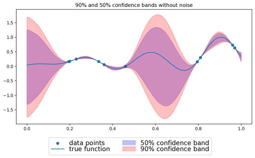
Figure 1: Nonparametric confidence bands for the noise-free setting.

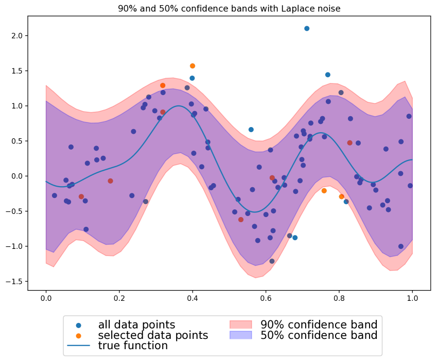
Figure 2: Nonparametric confidence bands with measurement noise.

6 Numerical Experiments

The algorithms were also tested numerically. We used a Paley-Wiener RKHS with $\eta=30$. The “true” function was constructed as follows: first, $20$ random input points $\{\bar{x}_{k}\}_{k=1}^{20}$ were generated, with uniform distribution on $[\hskip 0.85358pt0,1]$. Then $f_{*}(x)=\sum_{k=1}^{20}w_{k}k(x,\bar{x}_{k})$ was created, where each $w_{k}$ had a uniform distribution on $[-1,1]$. The function was normalized, in case its maximum exceeded $1$. Then, $n$ random observations were generated about $f_{*}$. In the noisy case, $\{\varepsilon_{k}\}$ had Laplace distribution with location $\mu=0$ and scale $b=0.4$ parameters.

In the noise-free case, we used $n=10$ observations, and created confidence bands with risk $\alpha=0.1$ and $0.5$. Figure 1 demonstrates that in the noise-free setting a very small sample size can lead to informative nonparametric confidence bands.

In case of measurement noises, $n=100$ sample size was used with $d=20$ (orange points). Confidence bands with risk $\alpha+\beta=0.1$ and $0.5$ are illustrated in Figure 2. We simply used $\alpha=\beta$ in these cases. The results indicated that even with limited information, adequate regions can be created.

7 Conclusions

In this paper a nonparametric and distribution-free method was introduced to build simultaneous confidence bands for bounded, band-limited functions. The construction was first presented for the case when there are no measurement noises, then it was extended allowing symmetric noises. Besides having non-asymptotic theoretical guarantees, the approach was also demonstrated numerically, supporting its feasibility.

References

- [1] F. Cucker and D. X. Zhou, Learning Theory: An Approximation Theory Viewpoint, vol. 24. Cambridge University Press, 2007.
- [2] L. Ljung, “Perspectives on System Identification,” Annual Reviews in Control, vol. 34, no. 1, pp. 1–12, 2010.
- [3] L. Györfi, M. Kohler, A. Krzyzak, and H. Walk, A Distribution-Free Theory of Nonparametric Regression. Springer, 2002.
- [4] A. Carè, B. Cs. Csáji, M. Campi, and E. Weyer, “Finite-Sample System Identification: An Overview and a New Correlation Method,” IEEE Control Systems Letters, vol. 2, no. 1, pp. 61 – 66, 2018.
- [5] J. Quinonero-Candela and C. E. Rasmussen, “A Unifying View of Sparse Approximate Gaussian Process Regression,” Journal of Machine Learning Research, vol. 6, pp. 1939–1959, 2005.
- [6] V. Vovk, A. Gammerman, and G. Shafer, Algorithmic Learning in a Random World. Springer Science & Business Media, 2005.
- [7] M. C. Campi, G. Calafiore, and S. Garatti, “Interval Predictor Models: Identification and Reliability,” Automatica, vol. 45, pp. 382–392, 2009.
- [8] S. Garatti, M. Campi, and A. Care, “On a Class of Interval Predictor Models with Universal Reliability,” Automatica, vol. 110, 2019.
- [9] G. Pillonetto, F. Dinuzzo, T. Chen, G. De Nicolao, and L. Ljung, “Kernel Methods in System Identification, Machine Learning and Function Estimation: A Survey,” Automatica, pp. 657–682, 2014.
- [10] A. Berlinet and C. Thomas-Agnan, Reproducing Kernel Hilbert Spaces in Probability and Statistics. Springer, 2004.
- [11] A. Iosevich and A. Mayeli, “Exponential Bases, Paley-Wiener Spaces and Applications,” Journal of Functional Analysis, pp. 363–375, 2015.
- [12] V. Vapnik, Statistical Learning Theory. Wiley-Interscience, 1998.
- [13] M. A. Pinsky, Introduction to Fourier Analysis and Wavelets, vol. 102. American Mathematical Society, 2008.
- [14] B. Cs. Csáji and K. B. Kis, “Distribution-Free Uncertainty Quantification for Kernel Methods by Gradient Perturbations,” Machine Learning, vol. 108, no. 8, pp. 1677–1699, 2019.
- [15] B. Cs. Csáji, M. C. Campi, and E. Weyer, “Sign-Perturbed Sums: A New System Identification Approach for Constructing Exact Non–Asymptotic Confidence Regions in Linear Regression models,” IEEE Transactions on Signal Processing, vol. 63, no. 1, pp. 169–181, 2014.
- [16] T. Hofmann, B. Schölkopf, and A. J. Smola, “Kernel Methods in Machine Learning,” Annals of Statistics, vol. 36, pp. 1171–1220, 2008.