Patch Selection for Melanoma Classification

Abstract

In medical image processing, the most important information is often located on small parts of the image. Patch-based approaches aim at using only the most relevant parts of the image. Finding ways to automatically select the patches is a challenge. In this paper, we investigate two criteria to choose patches: entropy and a spectral similarity criterion. We perform experiments at different levels of patch size. We train a Convolutional Neural Network on the subsets of patches and analyze the training time. We find that, in addition to requiring less preprocessing time, the classifiers trained on the datasets of patches selected based on entropy converge faster than on those selected based on the spectral similarity criterion and, furthermore, lead to higher accuracy. Moreover, patches of high entropy lead to faster convergence and better accuracy than patches of low entropy.

1 Introduction

With the development of better machine learning methods driven by deep learning, there have been many successful applications of neural networks in medical image processing, such as biomedical image segmentation or cancer diagnosis [1]. This is the case in cancer diagnosis and prognosis, with applications in breast cancer [22], lung cancer [14] and skin cancer [2].

Medical images can be widely different depending on their source, such as CT (Computed Tomography) scans, MRI (Magnetic Resonance Imaging) images, dermoscopy, etc. While classification is usually performed on the whole images, medical images can have extremely high resolution, e.g. gigapixels for skin tissue images, which makes it more time efficient to train on subsets or patches of images. Additionally, it can enhance a classifier performance in some settings. For example, in [11], the authors argue that cancer subtypes are distinguished at the image patch scale. Patch-based classification is also used in [18] for breast histology. More applications of patch-based applications are introduced in [17] and [25].

A judicious choice of patches reduces the importance of noise and focuses on the most important parts of the image. Two approaches of selecting the patches used for classification are to score the patches individually based on a given metric, or to compare each patch with the other patches of an image and rank the similarity between the patches. In the first approach, the patches can be scored using entropy, while the second approach relies on a similarity measure between images.

On one hand, entropy is used in information theory as a way to quantify the level of information of an object. Higher entropy means that there is more information in the object. For instance, a random noise image has high entropy while a unicolored one has very low entropy. Entropy plays an important role in data compression where it provides the lower bound on the storage required to compress an object without loss of information [19]. Entropy can also be used for object reconstruction using the principle of maximum entropy, which aims at selecting the most uniform probability distribution amongst multiple candidate distributions. It can be used for image reconstruction where the candidates are the set of missing pixels [20]. It applies to text data as well [15]. Entropy can also be used in image texture analysis [26] and texture synthesis. Selecting patches using entropy was explored in [13].

On the other hand, the Mean Exhaustive Minimum Distance (MEMD) is a criterion that was introduced in [8] to compare two images by trying to find the best pairing of pixels from the first and the second image; the criterion score then indicates how similar the images are. A low score indicates that the images are similar, and a high score that the image are different. This can be extended to comparison between a patch and several patches by averaging the scores.

In this paper we study the training time and the accuracy of these two criteria for patch-based binary classification. The data we use comes from the ISIC (International Skin Imaging Collaboration) archive. This consortium was created to improve the fight against skin melanoma cancer by improving computer-aided diagnosis. The consortium has held an annual challenge since 2016 [6]. Starting from 2019, the challenges are centered around dermoscopic image multi-class classification. The best team on the 2019 challenge [4], investigated patch-based classification on the HAM10000 dataset [21], where information from several patches is combined via an attention-based mechanism.

The paper is divided as follows. In Section 2 we present the dataset and the preprocessing we perform on the data. We also introduce the entropy and MEMD criterion that we use in our experiments. In Section 3 we present the results of our experiments and we conclude the paper in Section 4.

2 Materials and Methods

In this section we describe the dataset, the criteria of entropy and Mean-Exhaustive Minimum Distance (MEMD) we use, and the network architecture that is trained on the data.

2.1 Dataset description and preprocessing

The ISIC archive database comprises skin lesion images associated with a label indicating the status of the lesion. The image resolution is arbitrary. The archive provides an API to retrieve the images and their metadata, as well as the mask of the region of interest when an expert has created one. The total number of patches created is presented in Table 1. We perform binary classification on patches of the images. Our target variable is a categorical variable with two possible values: benign, or malignant.

The preprocessing steps are:

1. We download images from the ISIC archive, as well as the masks that are annotations from experts and indicate the lesion location.

2. All the malignant images with a mask are selected. The same number of benign images is sampled out of all the benign images.

3. The region of interest is divided in square patches of width 32, 64, 128 and 256. The region of interest is defined by the downloaded masks.

4. The entropy of each patch is computed, and we use these values to extract a subset of patches. This is explained in section 2.2.

5. For each image, we compute a spectral measure of similarity between a patch and all the other patches of the image; we use this measure to extract a subset of patches. The details are in section 2.3.

6. Finally, a classifier is trained on all the datasets we have created in the two previous steps.

Table 1: Number of patches for each patch size

Patch size	Number of patches
$32\times 32$	$4,889,969$
$64\times 64$	$1,173,052$
$128\times 128$	$270,821$
$256\times 256$	$58,253$

We divide the images in three groups: $90\%$ of the images are in the train set, with $20\%$ of the train set reserved for validation; the remaining $10\%$ constitutes the test set.

2.2 Entropy

We use the Shannon entropy [19]. It is defined by the formula

$$H=\sum_{k=1}^{M}p_{k}\log(p_{k})$$ (1)

where we sum across all the pixel intensities, i.e. from 0 to $M=255$. $p_{k}$ is the probability a pixel in the image is at intensity $k$. The entropy ranges from $0$ to $\log_{2}(255)\approx 8$. Because there is no consensus on how to compute the entropy for multi channel images, we convert our RGB images to grayscale. The conversion process is defined in the ITU-R Recommendation BT.601-2.

Using the entropy, we extract two datasets for each patch size:

• a low dataset, whose patches are all the patches that rank below the 15-th and the 30-th quantile of entropy with respect to the other patches of the same image.

• a high dataset, with entropy above the 85-th and the 70-th quantile.

2.3 Mean Exhaustive Minimum Distance (MEMD) criterion

The first methods of similarity measure usually consisted in computing certain features on a given image, such as the Haralick features [7], and then comparing the features obtained for different images. More recent techniques dealing with the structural similarity in textures have been proposed in [27] and [16]. Handling color or hyperspectral images is often done using histograms [24], but histograms require a large amount of data to get good estimates of the spectral distribution. A new criterion to evaluate the similarity of two images was proposed in [8]. This approach does not require histograms and generalizes to any number of channels.

Following the notation from [9], let $A$ and $B$ be two images, which can have multiple channels. Let $M=\min(\#A,\#B)$, with $\#A$ and $\#B$ the number of pixels in $A$ and $B$. Let $\langle A\rangle$ be the set of pairs of coordinates for the pixels of A, and $U$ the unprocessed pairs of coordinates of pixels of B. Let $\rho$ be the distance induced by a vector metric. $A_{i,j}$ denotes the pixel of $A$ at coordinates $(i,j)$; the channels dimension is implied. Similarly, $B_{k,l}$ is the pixel of $B$ at coordinates $(k,l)$. The MEMD criterion $\zeta$ is defined by Equation 2.

$$\zeta(A,B)=\frac{1}{M}\sum_{(i,j)\in\langle A\rangle}\min_{(k,l)\in U}\{\rho(A_{i,j},B_{k,l})\}$$ (2)

The lower the score is, the more similar images $A$ and $B$ are. Inversely, the higher the score, the higher the difference between the two images. The score can take values between 0 and 255. A score of 0 happens when we compare one image to itself; a score of 255 happens when we compare a white image with a black one.

To improve the computation time, [9] suggested that the pixels of both the images be sorted with respect to the chosen norm. Finding the minimum distance between the pixels of the two images then comes down to choosing the closest unprocessed neighbour in the sorted array. In the special case where $A$ and $B$ are of the same size, we can simply match the first element of the sorted pixels of $A$ with the first of element of the sorted pixels of $B$, and so on.

We compute the MEMD score of each patch with respect to all the other patches of the same image, and we average the scores. Figure 1 shows the distribution of the MEMD score at varying patch sizes. We observe two peaks. The peak on the left corresponds to the patches that are representative of the overall image, and the peak on the right corresponds to the patches that are more unique. The reason why we only have two peaks is that the images of the lesion all share similar elements: a little bit of skin, the lesion, and some noise such as hair, a ruler, etc. The distinction between the lesion and the skin is quite drastic, meaning that few patches are going to be equally similar to skin and lesion. The variation in scores is in part due to the different number of patches per image. The more patches an image has, the less extreme the MEMD score of the patches will be. The patches with a score of 0 are from images that have only one patch. This happens for big patch sizes where the region of interest is too small to get more patches.

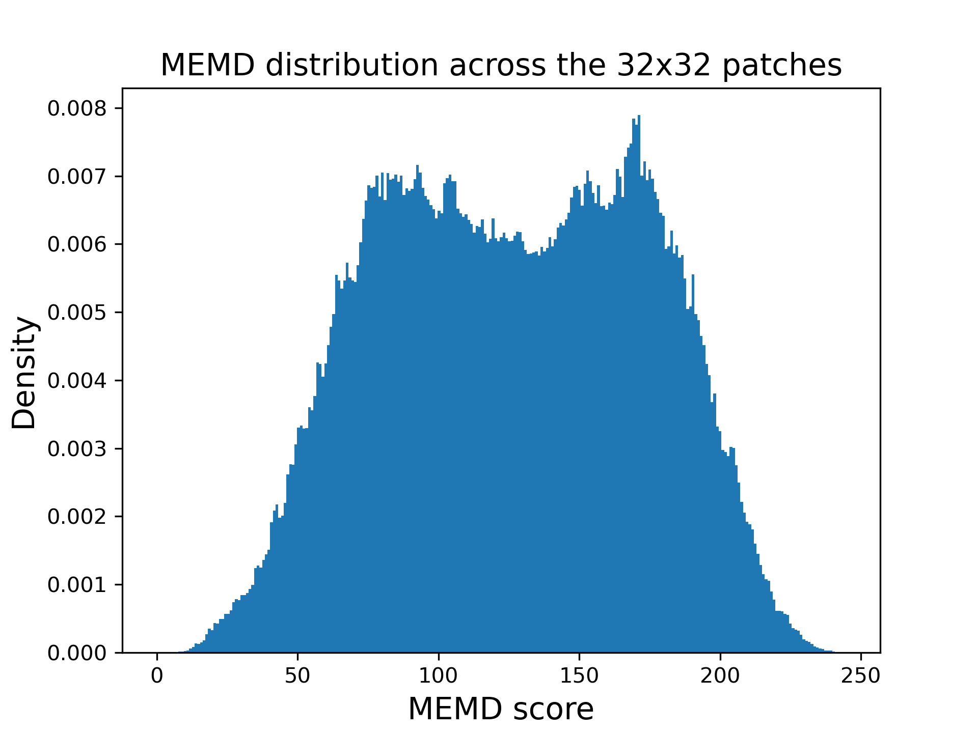
(a) $32\times 32$ patches

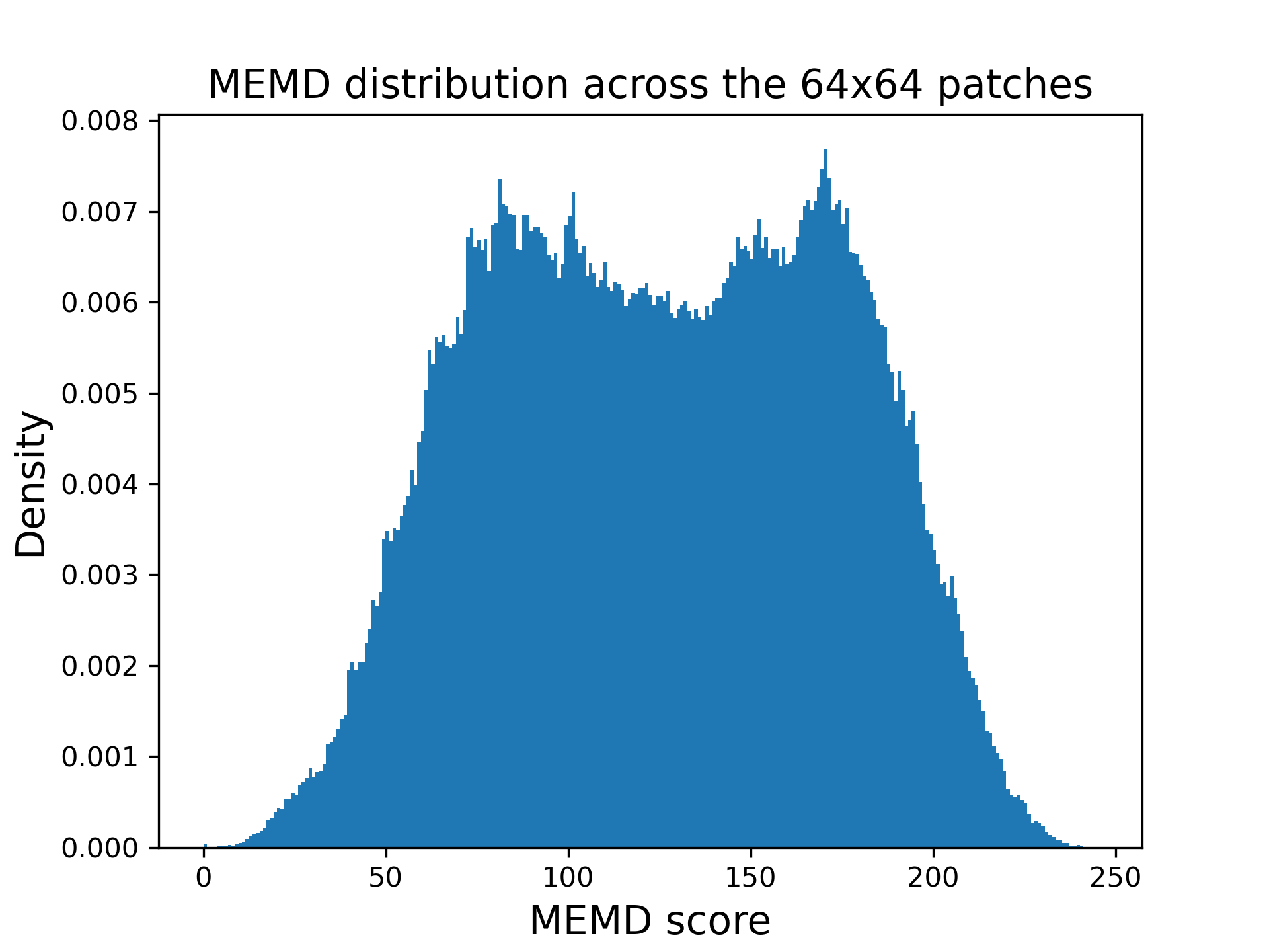
(b) $64\times 64$ patches

(c) $128\times 128$ patches

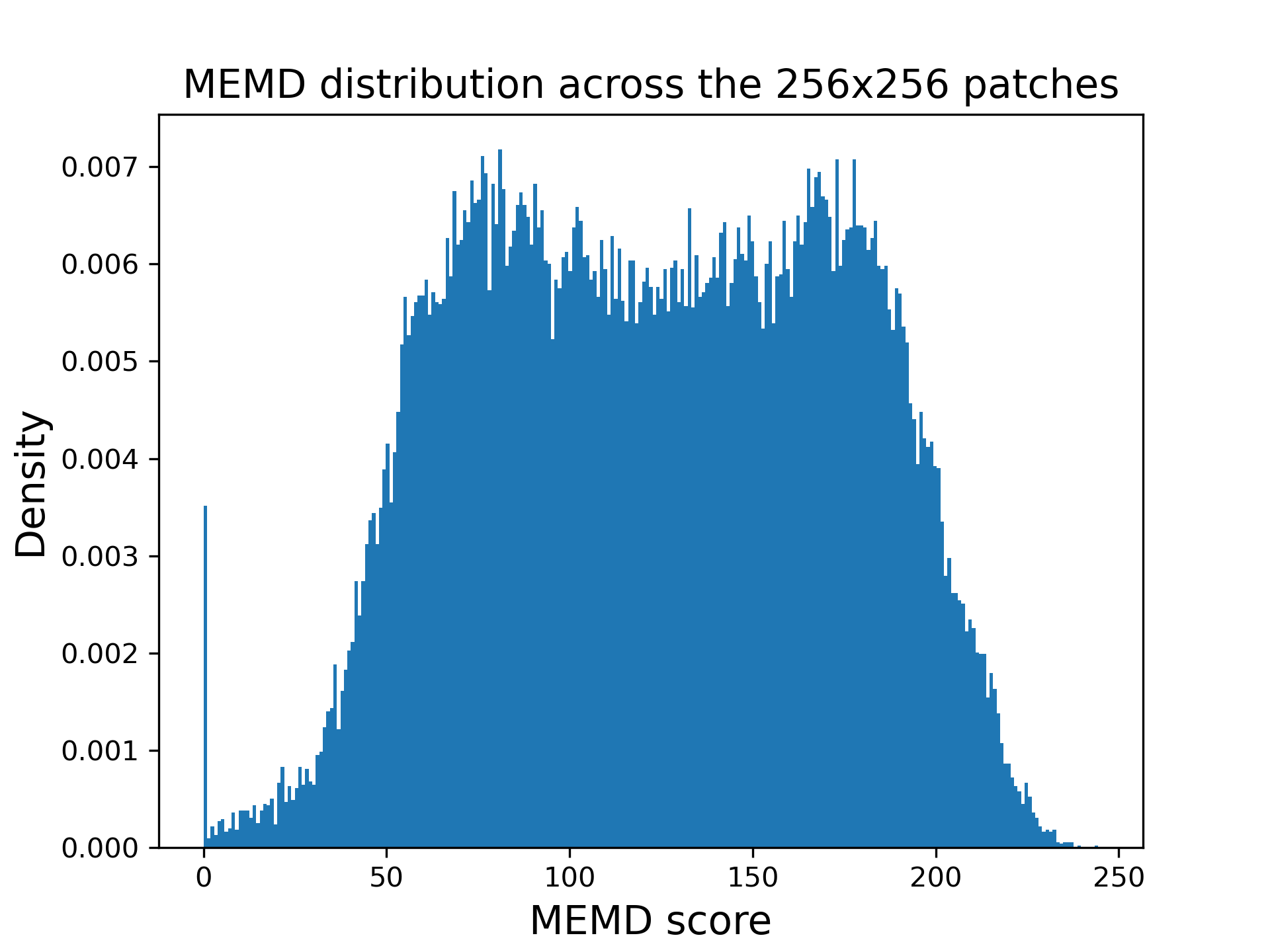
(d) $256\times 256$ patches

Figure 1: Distribution of MEMD score for different patch sizes

Similarly to what was done in Section2.2, we create datasets using the same quantiles for the MEMD score.

In the rest of the paper, we use the max norm for $\rho$, i.e. $\rho:x\mapsto\left\lVert x\right\rVert_{\infty}=\max_{i}\lvert x_{i}\rvert$, where $x_{i}$ are the coordinates of $x$. The distance induced by the max norm is $(x,y)\mapsto\left\lVert x-y\right\rVert_{\infty}$. Because the sorting of the pixels is done based on the norm of a single pixel, and the min is computed using the distance between two pixels, the optimization via sorting is not compatible with pixels with multiple channels. Indeed, let $p_{1}=[135,18,89]$, $p_{2}=[130,16,86]$ and $p_{3}=[12,134,1]$. If we sort the pixels by the max norm, we get $P=[p_{2},p_{3},p_{1}]$. Selecting the closest matching pixel using the proposed method in [9] would make us pair $p_{2}$ with $p_{3}$, which leads to $\zeta(p_{2},p_{3})=118$. But $p_{2}$ and $p_{1}$ are clearly a better match, with $\zeta(p_{2},p_{1})=5$. To alleviate the complications imposed by the multiple channels, we convert the images to grayscale before computing the MEMD score. Since the grayscale image has only one channel, the optimization via sorting works.

The computation of the average MEMD of all the patches of an image has $O(m^{2})$ with respect to $m$, the number of patches in the image. There is a trade-off between space and time complexity, where vectorizing part of the process using higher order tensors allows for faster computation but requires more space.

2.4 Network Architecture

For the choice of classifier, we follow [23] and [3] who found that ResNet50 achieved the best results for the same task and dataset. ResNet50 [10] is a 50-layer convolutional neural network (CNN) that was proposed to alleviate the problem of vanishing and exploding gradients [5] by introducing the notion of residual units.

With enough computing resources, ResNets can have as many layers as we want, e.g. 101 or 152 layers. We use the 50-layer version, which we adapt to binary classification by removing the last layer and replacing it with a max pooling layer followed by a Dense layer and a sigmoid activation.

We use the Adam optimizer [12]. We set the learning rate to $0.001$ and we use a binary cross-entropy loss for training.

We train the model for 10 epochs, each epoch representing a full pass through the train set.To mitigate overfitting, the training stops if the validation loss does not decrease after 3 consecutive epochs.

Additionally, we investigate combining predictions from several patches of an image to classify the image. We train a Resnet for 10 epochs and choose the weights that result in the best validation loss. To classify an image from the test set, we individually classify its patches and aggregate the results. Let $\mathcal{P}_{i}$ be the set of patches from an image $I_{i}$, $|\mathcal{P}_{i}|$ the number of patches selected from the image, $f$ be the classifier that maps a patch to $0$ for a benign patch and $1$ for a malignant one. The prediction $\hat{y}$ is given by the Equation 3.

$$\hat{y}_{i}=\begin{cases}0&\text{if }\left(\frac{1}{|\mathcal{P}|}\sum_{p\in\mathcal{P}_{i}}f(p)\right)<0.5\\ 1&\text{otherwise}\end{cases}$$ (3)

3 Experimental Results

The experiments were performed with an Nvidia Titan XP GPU. The code is written in Python and Tensorflow. The Pillow library was used for computing the entropy.

To make our results robust against the random initialization of the model parameters, we train 10 instances of a ResNet50 per dataset. Results of the experiments with the entropy datasets are presented in Table 2, and those performed on the MEMD datasets are presented in Table 3. The low entropy dataset contains the $15\%$ patches with the lowest entropy, and the high entropy dataset contains the $15\%$ patches with the highest entropy. Correspondingly, the low MEMD dataset contains the $15\%$ patches with the lowest MEMD score, and the high MEMD dataset contains the $15\%$ patches with the highest MEMD score. Additional results for datasets with intermediate entropy are presented in [13].

Table 2: Quantiles of training time for datasets of different entropy and patch size

		Quantile of training time (in seconds)
patch size	entropy	30	50 (median)	70
32	high	1350.7	2013.2	2781.4
32	low	1534.9	2906.7	3078.5
64	high	291.0	382.9	441.9
64	low	290.6	338.3	414.2
128	high	155.0	204.6	220.0
128	low	204.8	255.0	255.4
256	high	142.4	152.2	189.7
256	low	189.6	226.4	226.5

Table 3: Quantiles of training time for datasets of varying MEMD score and patch size

		Quantile of training time (in seconds)
patch_size	memd_score	30	50 (median)	70
32	high	3150.4	3254.8	3258.9
	low	3256.4	3260.0	3260.9
64	high	465.3	495.1	527.0
	low	564.4	691.9	986.3
128	high	241.5	281.9	387.9
	low	256.6	357.7	373.1
256	high	189.7	245.2	264.4
	low	215.4	226.7	275.2

Regarding the entropy datasets, we observe a tendency of faster convergence for datasets with higher entropy compared to datasets with lower entropy. Lower entropy means that the distribution of pixel intensity concentrates on fewer pixels than it does for higher entropy. This concentration makes for smoother textures, which might be harder for the classifier to learn. Higher entropy datasets have more salient features that more discernible and thus more easily learnable by the network.

As for the MEMD datasets, the dataset composed of patches with higher score tends to converge faster than the dataset with lower score. This might be explainable by the fact that a low MEMD score means a high similarity of the patch with the rest of the image, while a high score indicates a distinctive spectral texture compared with the other patches of the same image. Thus, the higher score patches capture the more unique features of the lesion, while the lower score patches are more representative of the overall texture of the lesion. The high representativeness of a patch might extend to patches of low score from another image, while the unique features are probably different between images. Therefore, the dataset with high score is richer in more unique patches, which provide more information than the similar patches contained in the lower score dataset. This, in turn, makes the network training converge faster for the dataset with higher score patches.

These interpretations are borne out by the results of the experiments presented in Table 4. For the $128\times 128$ patches, the accuracy does not improve when we select more patches: it stagnates around $50\%$. This indicates that this patch size is too small to properly discriminate the lesions. The problem is not about the number of patches but about the fact that small patches do not contain enough information to determine the status of the lesion. We believe that this situation holds also for even smaller patches, e.g. $32\times 32$ or $64\times 64$ patches. Conversely, for the case of $256\times 256$ patches, we remark that using too few patches results in very low accuracy (around $25\%$); however, the accuracy increases considerably when we select more patches ($30\%$ of $15\%$), achieving $71\%$ accuracy for patches of high entropy. This accuracy is similar to the $74\%$ accuracy obtained by the authors of [3] when training on the whole region of interest with a ResNet50.

Table 4: Test accuracy (in percentage) for the different datasets. For a given patch size, the test images are the same for each method.

Dataset	low MEMD	high MEMD	low entropy	high entropy
$128\times 128$, $15\%$ patches	46.7	50.5	46.2	52.7
$128\times 128$, $30\%$ patches	43.9	51.6	39.6	52.7
$256\times 256$, $15\%$ patches	27.2	26.3	25.1	32.0
$256\times 256$, $30\%$ patches	45.5	57.2	52.7	71.0

The lower accuracy for the low MEMD and low entropy datasets, compared with the high MEMD and entropy datasets, suggests that it is not sufficient to select more patches to reach a higher level of accuracy; it is also important to select appropriate patches.

(a) Malignant lesion

(b) Mask of the lesion

Figure 2: A malignant image and its mask

(a) Patch with low MEMD score

(b) Patch with high MEMD score

Figure 3: Two different MEMD patches

(a) Patch with low entropy score

(b) Patch with high entropy score

Figure 4: Two different entropy patches

Figure 3 and Figure 4 illustrate the role of MEMD and entropy in patch selection. The patch on the left of Figure 3 is one of the patches with the lowest MEMD score for the image, while the patch on the right has one of the highest scores. Due to the fact that the masks cannot perfectly capture the lesion, there will always be some part of the skin that will be present in the mask. Since the skin has more uniform texture than the lesion, it is likely that patches of skin will have the lowest score. Similarly, the patches with low entropy will have more uniform features, while the patches with higher entropy will have more salient ones, as in Figure 4.

The datasets extracted using the entropy converge faster than the datasets extracted with the MEMD criterion. We hypothesize that a likely explanation is that patches extracted with the entropy share similar distributions of pixels, albeit sometimes shifted. The entropy quantifies the distribution of pixel intensity: the higher the entropy, the closer the pixel distribution will be to the uniform distribution. Thus, the patches from entropy extracted datasets are similar across the images, and this similarity is learnable by the network. On the other hand, datasets extracted using the MEMD criterion do not provide any quantifiable information about the pixel distribution. Their score is only indicative of how representative the patch is with respect to the image. The network might thus be confronted with a wider variety of patches which lead to a longer training time.

4 Conclusion

We examined the role of entropy and the MEMD criteria on both CNN training time and classification efficiency for patch-based melanoma detection. The preprocessing is longer with the MEMD criterion because we have to compare patches two by two, whereas entropy requires a single computation per patch. We found that higher entropy leads to faster convergence than lower entropy; similarly, a higher MEMD score, which indicates that the patch does not resemble other patches from the same image, also leads to faster convergence. In terms of accuracy, the models trained on the higher entropy dataset or the higher MEMD are more performant than the models trained on the lower entropy or lower MEMD datasets. We also found that creating patch datasets using an absolute measure of information, such as entropy, makes the network train faster than when the datasets were created using a similarity measure. We also observed that patch size plays a significant role in the classifier accuracy, with small patches leading to poor results, regardless of the percentage of patches used.

References

- [1] Anwar, S.M., Majid, M., Qayyum, A., Awais, M., Alnowami, M., Khan, M.K.: Medical Image Analysis using Convolutional Neural Networks: A Review. Journal of Medical Systems 42(11), 226 (Nov 2018). https://doi.org/10.1007/s10916-018-1088-1
- [2] Esteva, A., Kuprel, B., Novoa, R.A., Ko, J., Swetter, S.M., Blau, H.M., Thrun, S.: Dermatologist-level classification of skin cancer with deep neural networks. Nature 542(7639), 115–118 (Feb 2017). https://doi.org/10.1038/nature21056
- [3] Favole, F., Trocan, M., Yilmaz, E.: Melanoma Detection Using Deep Learning. In: Nguyen, N.T., Hoang, B.H., Huynh, C.P., Hwang, D., Trawiński, B., Vossen, G. (eds.) Computational Collective Intelligence, vol. 12496, pp. 816–824. Springer International Publishing, Cham (2020). https://doi.org/10.1007/978-3-030-63007-2_64
- [4] Gessert, N., Nielsen, M., Shaikh, M., Werner, R., Schlaefer, A.: Skin lesion classification using ensembles of multi-resolution EfficientNets with meta data. MethodsX 7, 100864 (2020). https://doi.org/10.1016/j.mex.2020.100864
- [5] Glorot, X., Bengio, Y.: Understanding the difficulty of training deep feedforward neural networks. In: Teh, Y.W., Titterington, D.M. (eds.) Proceedings of the Thirteenth International Conference on Artificial Intelligence and Statistics, AISTATS 2010, Chia Laguna Resort, Sardinia, Italy, May 13-15, 2010. JMLR Proceedings, vol. 9, pp. 249–256. JMLR.org (2010)
- [6] Gutman, D., Codella, N.C.F., Celebi, E., Helba, B., Marchetti, M., Mishra, N., Halpern, A.: Skin Lesion Analysis toward Melanoma Detection: A Challenge at the International Symposium on Biomedical Imaging (ISBI) 2016, hosted by the International Skin Imaging Collaboration (ISIC). arXiv:1605.01397 [cs] (May 2016)
- [7] Haralick, R.M., Shanmugam, K., Dinstein, I.: Textural Features for Image Classification. IEEE Transactions on Systems, Man, and Cybernetics SMC-3(6), 610–621 (Nov 1973). https://doi.org/10.1109/TSMC.1973.4309314
- [8] Havlíček, M., Haindl, M.: Texture spectral similarity criteria. IET Image Processing 13(11), 1998–2007 (2019). https://doi.org/10.1049/iet-ipr.2019.0250
- [9] Havlíček, M., Haindl, M.: Optimized Texture Spectral Similarity Criteria. In: Wojtkiewicz, K., Treur, J., Pimenidis, E., Maleszka, M. (eds.) Advances in Computational Collective Intelligence, vol. 1463, pp. 644–655. Springer International Publishing, Cham (2021). https://doi.org/10.1007/978-3-030-88113-9_52
- [10] He, K., Zhang, X., Ren, S., Sun, J.: Deep Residual Learning for Image Recognition. In: 2016 IEEE Conference on Computer Vision and Pattern Recognition (CVPR). pp. 770–778. IEEE, Las Vegas, NV, USA (2016). https://doi.org/10.1109/CVPR.2016.90
- [11] Hou, L., Samaras, D., Kurc, T.M., Gao, Y., Davis, J.E., Saltz, J.H.: Patch-based convolutional neural network for whole slide tissue image classification. In: 2016 IEEE Conference on Computer Vision and Pattern Recognition (CVPR). pp. 2424–2433 (2016). https://doi.org/10.1109/CVPR.2016.266
- [12] Kingma, D.P., Ba, J.: Adam: A method for stochastic optimization. CoRR abs/1412.6980 (2015)
- [13] Lachaud, G., Céspedes, P.C., Trocan, M.: Entropy role on patch-based binary classification for skin melanoma. In: Wojtkiewicz, K., Treur, J., Pimenidis, E., Maleszka, M. (eds.) Advances in Computational Collective Intelligence - 13th International Conference, ICCCI 2021, Kallithea, Rhodes, Greece, September 29 - October 1, 2021, Proceedings. Communications in Computer and Information Science, vol. 1463, pp. 324–333. Springer (2021). https://doi.org/10.1007/978-3-030-88113-9_26, https://doi.org/10.1007/978-3-030-88113-9_26
- [14] Marentakis, P., Karaiskos, P., Kouloulias, V., Kelekis, N., Argentos, S., Oikonomopoulos, N., Loukas, C.: Lung cancer histology classification from CT images based on radiomics and deep learning models. Medical & Biological Engineering & Computing 59(1), 215–226 (Jan 2021). https://doi.org/10.1007/s11517-020-02302-w
- [15] Nigam, K., Lafferty, J., McCallum, A.: Using maximum entropy for text classification. In: IJCAI-99 Workshop on Machine Learning for Information Filtering. vol. 1, pp. 61–67. Stockholom, Sweden (1999)
- [16] Qin, X., Yang, Y.H.: Similarity measure and learning with gray level aura matrices (GLAM) for texture image retrieval. In: Proceedings of the 2004 IEEE Computer Society Conference on Computer Vision and Pattern Recognition, 2004. CVPR 2004. vol. 1, pp. I–I (Jun 2004). https://doi.org/10.1109/CVPR.2004.1315050
- [17] Rousseau, F., Habas, P.A., Studholme, C.: A supervised patch-based approach for human brain labeling. IEEE Trans. Medical Imaging 30(10), 1852–1862 (2011). https://doi.org/10.1109/TMI.2011.2156806
- [18] Roy, K., Banik, D., Bhattacharjee, D., Nasipuri, M.: Patch-based system for Classification of Breast Histology images using deep learning. Comput. Medical Imaging Graph. 71, 90–103 (2019). https://doi.org/10.1016/j.compmedimag.2018.11.003
- [19] Shannon, C.E.: A mathematical theory of communication. Bell System Technical Journal 27(3), 379–423 (1948). https://doi.org/10.1002/j.1538-7305.1948.tb01338.x
- [20] Skilling, J., Bryan, R.: Maximum entropy image reconstruction-general algorithm. Monthly notices of the royal astronomical society 211, 111 (1984)
- [21] Tschandl, P., Rosendahl, C., Kittler, H.: The HAM10000 dataset, a large collection of multi-source dermatoscopic images of common pigmented skin lesions. Scientific Data 5(1), 180161 (Dec 2018). https://doi.org/10.1038/sdata.2018.161
- [22] Yala, A., Lehman, C., Schuster, T., Portnoi, T., Barzilay, R.: A Deep Learning Mammography-Based Model for Improved Breast Cancer Risk Prediction. Radiology 292(1), 60–66 (Jul 2019). https://doi.org/10.1148/radiol.2019182716
- [23] Yilmaz, E., Trocan, M.: Benign and Malignant Skin Lesion Classification Comparison for Three Deep-Learning Architectures. In: Nguyen, N.T., Jearanaitanakij, K., Selamat, A., Trawiński, B., Chittayasothorn, S. (eds.) Intelligent Information and Database Systems, vol. 12033, pp. 514–524. Springer International Publishing, Cham (2020). https://doi.org/10.1007/978-3-030-41964-6_44
- [24] Yuan, J., Wang, D., Cheriyadat, A.M.: Factorization-Based Texture Segmentation. IEEE Transactions on Image Processing 24(11), 3488–3497 (Nov 2015). https://doi.org/10.1109/TIP.2015.2446948
- [25] Zhang, F., Song, Y., Cai, W., Lee, M.Z., Zhou, Y., Huang, H., Shan, S., Fulham, M.J., Feng, D.D.: Lung nodule classification with multilevel patch-based context analysis. IEEE Transactions on Biomedical Engineering 61(4), 1155–1166 (2014). https://doi.org/10.1109/TBME.2013.2295593
- [26] Zhu, S.C., Wu, Y.N., Mumford, D.: Minimax entropy principle and its application to texture modeling. Neural Computation 9(8), 1627–1660 (1997). https://doi.org/10.1162/neco.1997.9.8.1627
- [27] Zujovic, J., Pappas, T.N., Neuhoff, D.L.: Structural similarity metrics for texture analysis and retrieval. In: 2009 16th IEEE International Conference on Image Processing (ICIP). pp. 2225–2228. IEEE, Cairo, Egypt (Nov 2009). https://doi.org/10.1109/ICIP.2009.5413897