Triple electron-electron-proton excitations and second-order approximations in nuclear-electronic orbital coupled cluster methods

Abstract

The accurate description of nuclear quantum effects, such as zero-point energy, is important for modeling a wide range of chemical and biological processes. Within the nuclear-electronic orbital (NEO) approach, such effects are incorporated in a computationally efficient way by treating electrons and select nuclei, typically protons, quantum mechanically with molecular orbital techniques. Herein, we implement and test a NEO coupled cluster method that explicitly includes the triple electron-proton excitations, where two electrons and one proton are excited simultaneously. Our calculations show that this NEO-CCSD(eep) method provides highly accurate proton densities and proton affinities, outperforming any previously studied NEO method. These examples highlight the importance of the triple electron-electron-proton excitations for an accurate description of nuclear quantum effects. Additionally, we also implement and test the second-order approximate coupled cluster with singles and doubles (NEO-CC2) method, as well as its scaled-opposite-spin (SOS) versions. The NEO-SOS^′-CC2 method, which scales the electron-proton correlation energy as well as the opposite-spin and same-spin components of the electron-electron correlation energy, achieves nearly the same accuracy as the NEO-CCSD(eep) method for the properties studied. Because of its low computational cost, this method will enable a wide range of chemical and photochemical applications for large molecular systems. This work sets the stage for a wide range of developments and applications within the NEO framework.

I Introduction

Multicomponent quantum chemistry methods, in which more than one type of particle (e.g., electrons, positrons, nuclei, or photons) is treated quantum mechanically, are promising theoretical tools for describing various types of interesting chemical phenomena. Pavosevic, Culpitt, and Hammes-Schiffer (2020); Ruggenthaler et al. (2018); Pavošević et al. (2022) Among different multicomponent approaches,Ishimoto, Tachikawa, and Nagashima (2009); Pavosevic, Culpitt, and Hammes-Schiffer (2020); Reyes, Moncada, and Charry (2019) the nuclear-electronic orbital (NEO) method Webb, Iordanov, and Hammes-Schiffer (2002); Pavosevic, Culpitt, and Hammes-Schiffer (2020) treats all electrons and specified nuclei, typically protons, quantum mechanically on the same footing with molecular orbital techniques. In this way, many important nuclear quantum effects, such as zero-point energy, proton delocalization, and hydrogen tunnelling, as well as non-Born-Oppenheimer effects, are included during energy and reaction path calculations in a computationally efficient way.

The simplest method that can be formulated within the NEO framework is NEO-Hartree-Fock (NEO-HF), Webb, Iordanov, and Hammes-Schiffer (2002) in which the wave function is represented as a direct product of single electronic and single protonic Slater determinants. Because the NEO-HF method treats electrons and protons as uncorrelated particles, the predictions obtained from this method, such as proton densities and resulting properties, are highly inaccurate and unreliable. Pavošević, Culpitt, and Hammes-Schiffer (2018); Pavošević and Hammes-Schiffer (2019a); Pavosevic, Culpitt, and Hammes-Schiffer (2020) Analogous to conventional electronic structure methods, there are two main strategies to incorporate the missing correlation effects between quantum particles: density functional theory (DFT) Pak, Chakraborty, and Hammes-Schiffer (2007); Yang et al. (2017); Brorsen, Yang, and Hammes-Schiffer (2017) and wave function theory. Webb, Iordanov, and Hammes-Schiffer (2002); Nakai and Sodeyama (2003); Ishimoto, Tachikawa, and Nagashima (2009); Pavošević, Culpitt, and Hammes-Schiffer (2018); Pavošević and Hammes-Schiffer (2019a); Pavošević, Rousseau, and Hammes-Schiffer (2020); Pavošević, Tao, and Hammes-Schiffer (2021); Fajen and Brorsen (2020, 2021a) In the NEO-DFT method, both electron-electron and electron-proton correlation effects are included via correlation functionals in a computationally practical manner.Yang et al. (2017); Brorsen, Yang, and Hammes-Schiffer (2017) Because this method balances accuracy and computational cost, it is suitable for treatment of large molecular systems. However, a disadvantage of the NEO-DFT method is that it is not systematically improvable, and it suffers from the same problems that are inherent to conventional DFT methods,Hermann, DiStasio, and Tkatchenko (2017) such as self-interaction error. Cohen, Mori-Sánchez, and Yang (2008)

As an alternative to NEO-DFT, the wave function based methods, such as the NEO coupled cluster (NEO-CC) methods,Nakai and Sodeyama (2003); Ellis, Aggarwal, and Chakraborty (2016); Pavošević, Culpitt, and Hammes-Schiffer (2018); Pavošević and Hammes-Schiffer (2019a); Pavošević, Rousseau, and Hammes-Schiffer (2020); Pavošević, Tao, and Hammes-Schiffer (2021); Pavošević and Hammes-Schiffer (2021) are systematically improvable and parameter free. The NEO-CC methods use the exponentiated cluster operator to incorporate the correlation effects between quantum particles (i.e., electrons and protons) via single, double, and higher excitation ranks.Crawford and Schaefer (2000); Bartlett and Musiał (2007); Shavitt and Bartlett (2009) The truncation of the cluster operator up to a certain excitation rank establishes the NEO-CC hierarchy. For example, truncation of the cluster operator to include up to single and double electronic and protonic excitations, as well as double electron-proton excitations, defines the NEO coupled cluster with singles and doubles (NEO-CCSD) method.Pavošević, Culpitt, and Hammes-Schiffer (2018) Previously we showed that the NEO-CCSD method accurately predicts proton densities, energies, and vibrationally averaged geometries.Pavošević, Culpitt, and Hammes-Schiffer (2018); Pavošević and Hammes-Schiffer (2019a) More recently, the computational efficiency of the NEO-CCSD method was enhanced by the density fitting (DF) scheme,Pavošević, Tao, and Hammes-Schiffer (2021) which significantly reduces the memory requirements. This strategy enabled calculations of proton affinities of much larger molecules than previously possible, as well as the study of relative stabilities of protonated water tetramers with all nine protons treated quantum mechanically.Pavošević, Tao, and Hammes-Schiffer (2021) The reliability and robustness of the NEO-CCSD method has sparked an interest in development of other NEO wave function based methods, most notably the computationally attractive scaled-opposite-spin orbital optimized second-order Møller-Plesset perturbation theory (NEO-SOS^′-OOMP2) method,Pavošević, Rousseau, and Hammes-Schiffer (2020); Fetherolf et al. (2022) which scales the electron-proton correlation energy as well as the opposite-spin components of the electron-electron correlation energy.

In the NEO-CCSD method, truncation of the cluster operator to include up to double electron-proton excitations represented a compromise between accuracy and computational efficiency, as well as simplicity of implementation.Pavošević, Culpitt, and Hammes-Schiffer (2018) In order to account for some of the missing electron-proton correlation, in our previous work we used a larger electronic basis set for the quantum proton(s) than for the other nuclei.Pavošević, Culpitt, and Hammes-Schiffer (2018) Although this strategy works well by providing accurate predictions of different properties for the studied systems,Pavošević, Culpitt, and Hammes-Schiffer (2018); Pavošević and Hammes-Schiffer (2019a); Pavošević, Tao, and Hammes-Schiffer (2021) it might not be general for all systems. In this work, we move beyond the NEO-CCSD method by implementing the NEO-CCSD(eep) method, which also includes electron-electron-proton triple excitations. The importance of such triple excitations was observed recently in the context of perturbation theory.Fajen and Brorsen (2021b) Additionally, we implement and investigate a novel and computationally efficient second-order approximate coupled cluster with singles and doubles (NEO-CC2) method and its scaled-opposite-spin version (NEO-SOS^′-CC2). Analogous to its electronic counterpart,Christiansen, Koch, and Jørgensen ; Hellweg, Grün, and Hättig (2008); Tajti and Szalay (2019) the NEO-CC2 method can be used as a computationally efficient alternative to the equation-of-motion coupled cluster methods for excited states.Pavošević and Hammes-Schiffer (2019b); Pavošević et al. (2020) Moreover, in order to calculate protonic densities with these methods, we also implement the $\Lambda$-equations using automatic differentiation.Pavošević and Hammes-Schiffer (2020) The developments and tests performed within this work highlight the robustness and reliability of the NEO-CC methods.

II Theory

In this section we describe the multicomponent wave function approaches in which electrons and protons are treated quantum mechanically. We note that the extension to other multicomponent fermionic systems, such as where positrons instead of protons are treated quantum mechanically, is straightforward.Pavosevic, Culpitt, and Hammes-Schiffer (2020)

The NEO coupled cluster correlation energy is calculated from the energy Lagrangian asPavošević and Hammes-Schiffer (2019a)

$$E_{\text{NEO-CC}}=\langle 0^{\text{e}}0^{\text{p}}|(1+\hat{\Lambda})e^{-\hat{T}}\hat{H}_{\text{NEO}}e^{\hat{T}}|0^{\text{e}}0^{\text{p}}\rangle.$$ (1)

In this equation, $\hat{H}_{\text{NEO}}$ is the second-quantized normal-ordered (with respect to the NEO-HF reference state, $|0^{\text{e}}0^{\text{p}}\rangle$) NEO Hamiltonian that is expressed as

$$\hat{H}_{\text{NEO}}=F^{p}_{q}a^{q}_{p}+\frac{1}{4}\overline{g}^{pq}_{rs}a^{rs}_{pq}+F^{P}_{Q}a^{Q}_{P}+\frac{1}{4}\overline{g}^{PQ}_{RS}a^{RS}_{PQ}-g^{pP}_{qQ}a^{qQ}_{pP},$$ (2)

where $a_{p_{1}p_{2}...p_{n}}^{q_{1}q_{2}...q_{n}}=a_{q_{1}}^{\dagger}a_{q_{2}}^{\dagger}...a_{q_{n}}^{\dagger}a_{p_{n}}...a_{p_{2}}a_{p_{1}}$ are normal-ordered second-quantized excitation operators written in terms of fermionic creation/annihilation ($a^{\dagger}/a$) operators. The lowercase indices $i,j,k,l,...$, $a,b,c,d,...$, and $p,q,r,s,...$ denote occupied, unoccupied, and general electronic spin orbitals, whereas the corresponding uppercase indices denote protonic orbitals. Additionally, $F^{p}_{q}=\langle q|\hat{F}^{\text{e}}|p\rangle$ is a matrix element of the electronic Fock operator and $\overline{g}^{pq}_{rs}=g^{pq}_{rs}-g^{qp}_{rs}=\langle rs|pq\rangle-\langle rs|qp\rangle$ is an antisymmetrized two-electron repulsion tensor element. Their protonic counterparts $F^{P}_{Q}$ and $\overline{g}^{PQ}_{RS}$ are defined analogously, and $g^{pP}_{qQ}=\langle qQ|pP\rangle$ is the electron-proton attraction tensor element. The Einstein summation convention over repeated indices is utilized throughout this manuscript.

In Eq. (1), $\hat{T}=t_{\mu}a^{\mu}$ and $\hat{\Lambda}=\lambda^{\mu}a_{\mu}$ are excitation and de-excitation cluster operators, respectively, where $a^{\mu}=a_{\mu}^{\dagger}=\{a_{i}^{a},a_{I}^{A},a_{iI}^{aA},a_{ij}^{ab},a_{IJ}^{AB},a_{ijI}^{abA},a_{iIJ}^{aAB},...\}$ is a set of single, double, and higher excitation operators, and $\mu$ is an excitation rank. Moreover, $t_{\mu}$ and $\lambda^{\mu}$ are unknown wave function parameters (amplitudes) that are determined by minimizing Eq. (1) with respect to $\lambda^{\mu}$ and $t_{\mu}$, respectively:

$$\frac{\partial E_{\text{NEO-CC}}}{\partial\lambda^{\mu}}=\langle 0^{\text{e}}0^{\text{p}}|a_{\mu}e^{-\hat{T}}\hat{H}_{\text{NEO}}e^{\hat{T}}|0^{\text{e}}0^{\text{p}}\rangle=0,$$ (3)

$$\frac{\partial E_{\text{NEO-CC}}}{\partial t_{\mu}}=\langle 0^{\text{e}}0^{\text{p}}|(1+\hat{\Lambda})[e^{-\hat{T}}\hat{H}_{\text{NEO}}e^{\hat{T}},a^{\mu}]|0^{\text{e}}0^{\text{p}}\rangle=0.$$ (4)

The last two equations are known as the $t$-amplitude equations and the $\Lambda$-equations, respectively. The truncation of the cluster operator $\hat{T}$ up to a certain excitation rank $\mu$ establishes the NEO-CC hierarchy.

In our previous work,Pavošević, Culpitt, and Hammes-Schiffer (2018); Pavošević and Hammes-Schiffer (2019a); Pavošević, Tao, and Hammes-Schiffer (2021) the cluster operator $\hat{T}$ was defined as

$$\hat{T}^{\text{(ep)}}=t^{i}_{a}a_{i}^{a}+t^{I}_{A}a_{I}^{A}+t^{iI}_{aA}a_{iI}^{aA}+\frac{1}{4}t^{ij}_{ab}a_{ij}^{ab}+\frac{1}{4}t^{IJ}_{AB}a_{IJ}^{AB}.$$ (5)

Because the highest level of electron-proton excitation is the simultaneous single electronic and single protonic excitations due to $a_{iI}^{aA}$, we will refer to this method as NEO-CCSD(ep) throughout this manuscript. In the present work, we implement and explore the NEO-CC method with the cluster operator defined as

$$\hat{T}^{\text{(eep)}}=t^{i}_{a}a_{i}^{a}+t^{I}_{A}a_{I}^{A}+t^{iI}_{aA}a_{iI}^{aA}+\frac{1}{4}t^{ij}_{ab}a_{ij}^{ab}+\frac{1}{4}t^{IJ}_{AB}a_{IJ}^{AB}+\frac{1}{4}t^{ijI}_{abA}a_{ijI}^{abA}.$$ (6)

This cluster operator explicitly includes simultaneous double electronic and single protonic excitations. Although the total excitation rank of the operator $a_{ijI}^{abA}$ is triple, the highest excitation rank of a single particle (in this case electrons) is double, and therefore this method is denoted NEO-CCSD(eep). Although the addition of one extra term into the cluster operator may seem to be a trivial extension, the $t$-amplitude equations of the new NEO-CCSD(eep) method have roughly four times more terms than the NEO-CCSD(ep) method. Therefore, the derivation and implementation of the working equations for the NEO-CCSD(eep) method require a significant amount of effort. The computational cost of the NEO-CCSD(ep) and NEO-CCSD(eep) methods scales as $\mathcal{O}(N^{6})$, where $N$ is a measure of the system size, although the NEO-CCSD(eep) method has a greater prefactor than the NEO-CCSD(ep) method. For electron-dominated systems with one quantum-proton (as considered in the present study), the majority of the computation time for the NEO-CCSD(ep) method is spent in determining the $t^{ij}_{ab}$ amplitudes. On the other hand, the NEO-CCSD(eep) method has an additional set of $t$-amplitude equations for determining the $t^{ijI}_{abA}$ amplitudes. The total cost for the NEO-CCSD(eep) method is expressed roughly as the cost of determining the $t^{ij}_{ab}$ amplitudes multiplied by the number of protonic basis functions.

The programmable expressions for the $t$-amplitude equations of the NEO-CCSD(eep) method are obtained by utilizing the generalized Wick’s theorem.Kutzelnigg and Mukherjee (1997); Shavitt and Bartlett (2009); Bartlett and Musiał (2007) The $\Lambda$-equations can in principle be derived in the same way,Pavošević and Hammes-Schiffer (2019a) but because they have 50% more terms than the $t$-amplitude equations,Pavošević and Hammes-Schiffer (2019a, 2020) their derivation and implementation is a daunting task. Alternatively, the unknown $\lambda^{\mu}$ amplitudes can be calculated with the aid of automatic differentiation, as illustrated in our previous work.Pavošević and Hammes-Schiffer (2020) Within this procedure, the Lagrangian given in Eq. (1) is constructed by augmenting the NEO-CC energy $\big{(}\langle 0^{\text{e}}0^{\text{p}}|e^{-\hat{T}}\hat{H}_{\text{NEO}}e^{\hat{T}}|0^{\text{e}}0^{\text{p}}\rangle\big{)}$ with the $t$-amplitude equations from Eq. (3) weighted by the Lagrange multipliers $\lambda^{\mu}$. Therefore, if the $t$-amplitude equations are available, construction of the Lagrangian is straightforward. Once the Lagrangian is available, both $t_{\mu}$ and $\lambda^{\mu}$ are calculated with automatic differentiation. A significant advantage of this procedure is that it does not require derivation and implementation of the $\Lambda$-equations, thereby immensely reducing the coding effort.

The calculated wave function parameters $t_{\mu}$ and $\lambda^{\mu}$ allow calculation of various important molecular properties, one of which is the proton density that is used to validate the accuracy of NEO methods.Pavošević and Hammes-Schiffer (2019a) Accurate proton densities are crucial for calculation of molecular properties, such as vibrationally averaged geometries and zero-point energies.Brorsen, Yang, and Hammes-Schiffer (2017); Pavosevic, Culpitt, and Hammes-Schiffer (2020) The proton density is calculated from

$$\rho_{\text{p}}(\textbf{r}_{\text{p}})=\sum_{PQ}\gamma_{P}^{Q}\phi_{P}(\textbf{r}_{\text{p}})\phi_{Q}(\textbf{r}_{\text{p}}),$$ (7)

where $\gamma_{P}^{Q}$ is the total one-particle reduced density matrix that is defined as $\gamma_{P}^{Q}=\gamma_{\text{NEO-HF}}+\tilde{\gamma}_{P}^{Q}$. Here, $\gamma_{\text{NEO-HF}}$ is the NEO-HF one-particle reduced density matrix, and $\tilde{\gamma}_{P}^{Q}$ is the NEO-CC one-particle reduced density matrix defined by

$$\tilde{\gamma}_{P}^{Q}=\langle 0^{\text{e}}0^{\text{p}}|(1+\Lambda)e^{-\hat{T}}a_{P}^{Q}e^{\hat{T}}|0^{\text{e}}0^{\text{p}}\rangle.$$ (8)

In Eq. (7), $\phi_{P}$ is a protonic orbital and $\textbf{r}_{\text{p}}$ is the proton coordinate.

In this work, we also explore the second-order coupled cluster (NEO-CC2) method within the NEO framework, which can be regarded as an approximate NEO-CCSD(ep) method. In the NEO-CC2 method, the singles $t$-amplitude equations remain the same and are equivalent to those of the NEO-CCSD(ep) method, whereas the doubles $t$-amplitude equations are approximated as

$$\langle 0^{\text{e}}0^{\text{p}}|a_{\mu_{2}}\big{(}\bar{H}+[\hat{F},\hat{T}_{2}]\big{)}|0^{\text{e}}0^{\text{p}}\rangle=0.$$ (9)

Here, $a_{\mu_{2}}=\{a^{iI}_{aA},a^{ij}_{ab},a^{IJ}_{AB}\}$ is the double de-excitation operator, $\bar{H}=e^{-\hat{T}_{1}}\hat{H}_{\text{NEO}}e^{\hat{T}_{1}}$ is the normal-ordered $\hat{T}_{1}$-similarity transformed NEO Hamiltonian, and $\hat{F}=F^{p}_{q}a^{q}_{p}+F^{P}_{Q}a^{Q}_{P}$ is the normal-ordered second-quantized Fock operator. The cluster operators used in this expression are defined as

$$\hat{T}_{1}=t^{i}_{a}a_{i}^{a}+t^{I}_{A}a_{I}^{A}$$ (10)

and

$$\hat{T}_{2}=t^{iI}_{aA}a_{iI}^{aA}+\frac{1}{4}t^{ij}_{ab}a_{ij}^{ab}+\frac{1}{4}t^{IJ}_{AB}a_{IJ}^{AB}.$$ (11)

Due to the approximations introduced in the NEO-CC2 method, the computational cost scales as $\mathcal{O}(N^{5})$.

The NEO-CC2 method is closely related to the NEO-MP2 and NEO-OOMP2 methods. The NEO-MP2 method is obtained by setting the singles amplitudes in the NEO-CC2 method to zero, whereas the NEO-OOMP2 method is obtained by using the unitary rotations of orbitals instead of the exponentiated singles operator. The working equations of the NEO-CC2 and NEO-OOMP2 methods are very similar, as discussed in the context of their purely electronic counterparts in Ref. 33. Calculations of the $\Lambda$-equations and protonic density are performed analogously with the NEO-CC2 method as with the NEO-CCSD(ep) and NEO-CCSD(eep) methods.

The computational efficiency and accuracy of the NEO-CC2 method can be enhanced with the SOS approach, Jung et al. (2004); Distasio Jr and Head-Gordon (2007); Hellweg, Grün, and Hättig (2008); Tajti and Szalay (2019) in which the opposite-spin and same-spin components of the electron-electron correlation energy are scaled differently. In the context of the NEO method, the accuracy can be further enhanced by scaling the electron-proton contribution of the correlation energy,Pavošević, Rousseau, and Hammes-Schiffer (2020) leading to the NEO-SOS^′-CC2 method. Within this approach, the working singles and doubles amplitude equations are modified as follows:

$$\langle 0^{\text{e}}0^{\text{p}}|a_{\mu_{1}}\big{(}\bar{H}+\sum_{\sigma,\sigma^{\prime}}c_{\sigma,\sigma^{\prime}}[\bar{H},\hat{T}_{2,\text{ee}}^{\sigma,\sigma^{\prime}}]+c_{\text{ep}}[\bar{H},\hat{T}_{2,\text{ep}}]\big{)}|0^{\text{e}}0^{\text{p}}\rangle=0,$$ (12)

$$\langle 0^{\text{e}}0^{\text{p}}|a_{\mu_{2}}\big{(}\bar{H}+\sum_{\sigma,\sigma^{\prime}}c_{\sigma,\sigma^{\prime}}[\hat{F},\hat{T}_{2,\text{ee}}^{\sigma,\sigma^{\prime}}]+c_{\text{ep}}[\hat{F},\hat{T}_{2,\text{ep}}]\big{)}|0^{\text{e}}0^{\text{p}}\rangle=0,$$ (13)

respectively. The NEO-SOS^′-CC2 energy is calculated from

$$\begin{split}E_{\text{NEO-SOS${}^{\prime}$-CC2}}=&\langle 0^{\text{e}}0^{\text{p}}|\big{(}\bar{H}+\sum_{\sigma,\sigma^{\prime}}c_{\sigma,\sigma^{\prime}}[\bar{H},\hat{T}_{2,\text{ee}}^{\sigma,\sigma^{\prime}}]\\ &+c_{\text{ep}}[\bar{H},\hat{T}_{2,\text{ep}}]\big{)}|0^{\text{e}}0^{\text{p}}\rangle.\end{split}$$ (14)

In the last three equations, $\sigma$/$\sigma^{\prime}$ indicates $\alpha$/$\beta$ electron spin, $c_{\sigma,\sigma^{\prime}}=\{c_{\text{os}}=c_{\alpha\beta}=c_{\beta\alpha},c_{\text{ss}}=c_{\alpha\alpha}=c_{\beta\beta}\}$ are electron spin-specific scaling coefficients, $\hat{T}_{2,\text{ee}}^{\sigma,\sigma^{\prime}}=\frac{1}{2}t^{i_{\sigma}j_{\sigma^{\prime}}}_{a_{\sigma}b_{\sigma^{\prime}}}a_{i_{\sigma}j_{\sigma^{\prime}}}^{a_{\sigma}b_{\sigma^{\prime}}}$ is the spin-specific purely electronic cluster operator, $\hat{T}_{2,\text{ep}}=t^{iI}_{aA}a_{iI}^{aA}$ is the electron-proton cluster operator, and $c_{\text{ep}}$ is the scaling coefficient for the electron-proton correlation energy contribution. In the conventional electronic structure SOS-CC2 method, the opposite-spin and the same-spin scaling parameters are $c_{\text{os}}=1.3$ and $c_{\text{ss}}=0.0$, respectively. Jung et al. (2004); Tajti and Szalay (2019) Neglecting the same-spin electron-electron correlation allows implementation of the SOS-CC2 and NEO-SOS^′-CC2 methods with $\mathcal{O}(N^{4})$ scaling. Jung et al. (2004); Tajti and Szalay (2019)

Throughout this work, we apply density fitting Whitten (1973); Dunlap, Connolly, and Sabin (1979) to approximate the four-center two-particle integrals from Eq. (2) asMejía-Rodríguez and de la Lande (2019); Pavošević, Tao, and Hammes-Schiffer (2021)

$$\begin{split}g^{pq}_{rs}&=(rp|sq)\\ &\approx\sum_{MN}(rp|M)(M|N)^{-1}(N|sq),\end{split}$$ (15a)

$$\begin{split}g^{PQ}_{RS}&=(RP|SQ)\\ &\approx\sum_{M^{\prime}N^{\prime}}(RP|M^{\prime})(M^{\prime}|N^{\prime})^{-1}(N^{\prime}|SQ),\end{split}$$ (15b)

$$\begin{split}g^{pP}_{qQ}&=(pq|QP)\\ &\approx\sum_{M^{\prime}N^{\prime}}(pq|M^{\prime})(M^{\prime}|N^{\prime})^{-1}(N^{\prime}|QP).\end{split}$$ (15c)

In these equations, $M$ and $N$ indices denote auxiliary electronic basis functions, and $M^{\prime}$ and $N^{\prime}$ indices denote auxiliary protonic basis functions. Within the density fitting approach, the four-center two-particle integrals (here expressed in the chemist notation) are approximated in terms of the three-center and two-center two-particle integrals, thereby significantly reducing the memory requirements.

III Results

The NEO-CCSD(ep), NEO-CCSD(eep), NEO-CC2, and NEO-SOS^′-CC2 methods were implemented in an in-house version of the Psi4NumPy quantum chemistry software. Smith et al. (2018) All the implemented methods rely on the density fitting scheme for approximating the four-center two-particle integrals. The programmable expressions of the $t$-amplitude equations for the NEO-CCSD(eep) method have been derived with the SeQuant software. Valeev (2014) The $\Lambda$-equations were solved using automatic differentiation with the procedure described elsewhere. Pavošević and Hammes-Schiffer (2020) Automatic differentiation was performed using the TensorFlow v2.1.0 program. Abadi et al. (2015) The NEO methods were used to calculate proton densities for the FHF^- and HCN molecules, as well as proton affinities for a set of 12 small molecules. Pavošević, Culpitt, and Hammes-Schiffer (2018) All of the calculations were performed at the equilibrium geometries optimized with the conventional electronic CCSD/aug-cc-pVTZ level of theory. In the present study, the calculations employed the aug-cc-pVXZ Dunning Jr (1989); Kendall, Dunning Jr, and Harrison (1992) electronic basis set along with its matching aug-cc-pVXZ-RI Weigend et al. (1998); Weigend, Köhn, and Hättig (2002) electronic auxiliary basis set, where the basis set cardinal number is X=D,T,Q,5. Moreover, the quantum protons were treated with the PB4-F2 (4s3p2d2f) nuclear basis set Yu, Pavošević, and Hammes-Schiffer (2020) as well with an even-tempered 8s8p8d8f auxiliary nuclear basis set with exponents ranging from 2$\sqrt{2}$ to 32. Culpitt et al. (2019) The electronic and nuclear basis sets for the quantum hydrogen were centered at the hydrogen position optimized with the CCSD method.

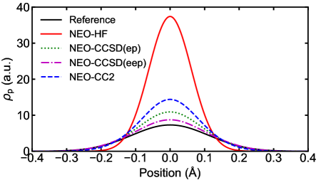
Figure 1: On-axis proton density for the FHF^- molecule calculated with the reference FGH (black solid curve), NEO-HF (red solid curve), NEO-CC2 (blue dashed curve), NEO-CCSD(ep) (green dotted curve), and NEO-CCSD(eep) (mangenta dashed-dotted curve) methods. The NEO calculations employ the aug-cc-pV5Z electronic basis set. The fluorine atoms are positioned at -1.1335 Å and 1.1335 Å, and the proton basis functions are centered at the origin. The on-axis proton density is along the line that connects the two fluorine atoms.

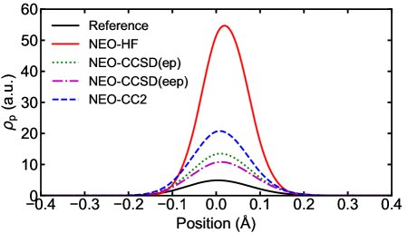
Figure 2: On-axis proton density for the HCN molecule calculated with the reference FGH (black solid curve), NEO-HF (red solid curve), NEO-CC2 (blue dashed curve), NEO-CCSD(ep) (green dotted curve), and NEO-CCSD(eep) (mangenta dashed-dotted curve) methods. The NEO calculations employ the aug-cc-pV5Z electronic basis set. The carbon atom is positioned at -1.058 Å, the nitrogen atom is positioned at -2.206 Å. and the proton basis functions are centered at the origin. The on-axis proton density is along the line that connects the carbon and nitrogen atoms.

Table 1: Root-Mean-Square deviation (RMSD) values of the proton density calculated with a NEO method relative to the FGH reference density.

	FHF-				HCN
method	aDZ	aTZ	aQZ	a5Z	aDZ	aTZ	aQZ	a5Z
NEO-HF	0.75	0.75	0.73	0.73	0.75	0.75	0.74	0.73
NEO-CCSD(ep)	0.41	0.26	0.15	0.13	0.48	0.36	0.25	0.23
NEO-CCSD(eep)	0.39	0.21	0.08	0.06	0.46	0.32	0.20	0.18
NEO-CC2	0.44	0.33	0.25	0.23	0.50	0.43	0.36	0.34
NEO-SOS-CC2	0.45	0.34	0.26	0.24	0.51	0.44	0.37	0.35
NEO-SOS′-CC2	-	-	0.06	-	-	-	0.18	-

To assess the accuracy of the novel NEO methods, we computed the proton densities for the FHF^- molecule and the HCN molecule. The benchmark densities were calculated with the Fourier Grid Hamiltonian (FGH) method, Webb and Hammes-Schiffer (2000) which is numerically nearly exact for these two systems. The FGH reference density was obtained at the conventional CCSD/aug-cc-pVDZ level of theory. For consistency with these NEO calculations, in the FGH method, only the hydrogen was treated quantum mechanically and the other nuclei were fixed. Figures 1 and 2 show on-axis one-dimensional slices of the proton densities for these two molecules calculated with the NEO-HF, NEO-CC2, NEO-CCSD(ep), NEO-CCSD(eep), and FGH methods. The on-axis proton density is along the line that connects the heavy atoms, which are either two fluorine atoms (for FHF^-) or carbon and nitrogen atoms (for HCN). Both the NEO and FGH three-dimensional proton densities are normalized to unity.

To quantify the difference between the proton densities obtained with the NEO methods and the FGH method, we computed the root-mean-square deviations (RMSDs). The RMSD values for both the FHF^- and HCN molecules calculated with the NEO-HF, NEO-CCSD(ep), NEO-CCSD(eep), NEO-CC2, and NEO-SOS^′-CC2 methods and with different basis sets are given in Table 1. As discussed previously,Pavošević, Culpitt, and Hammes-Schiffer (2018); Pavosevic, Culpitt, and Hammes-Schiffer (2020) the NEO-HF method produces proton densities that are too localized, mainly due to the inadequacies of the mean-field description. This behavior is depicted by the solid red curves in Figs. 1 and 2. Additionally, Table 1 shows that the NEO-HF exhibits the largest RMSD values, which remain nearly constant with increase of the basis set size.

Table 2: Absolute Deviation and Mean Unsigned Error (MUE) of Proton Affinities (in electron volts) with Respect to Experimental Data.

		NEO-CCSD(ep)				NEO-CCSD(eep)				NEO-CC2				NEO-SOS′-CC2
molecule	experiment	aDZ	aTZ	aQZ	a5Z	aDZ	aTZ	aQZ	a5Z	aDZ	aTZ	aQZ	a5Z	aQZ
CN-	15.31	0.58	0.30	0.24	0.18	0.55	0.26	0.18	0.12	0.71	0.46	0.43	0.38	0.01
NO${}_{2}^{-}$	14.75	0.40	0.20	0.13	0.08	0.36	0.15	0.06	$<$0.01	0.76	0.59	0.53	0.49	0.03
NH3	8.85	0.35	0.20	0.11	0.05	0.32	0.16	0.06	$<$0.01	0.47	0.35	0.29	0.24	0.08
HCOO-	14.97	0.42	0.22	0.12	0.05	0.39	0.18	0.07	0.01	0.74	0.58	0.51	0.43	0.02
HO-	16.95	0.46	0.21	0.12	0.05	0.42	0.16	0.05	0.02	0.83	0.64	0.58	0.54	0.11
HS-	15.31	0.55	0.32	0.25	0.14	0.52	0.27	0.18	0.07	0.74	0.51	0.47	0.38	0.04
H2O	7.16	0.42	0.23	0.16	0.10	0.39	0.19	0.10	0.05	0.55	0.39	0.33	0.29	$<$0.01
H2S	7.31	0.34	0.20	0.13	0.04	0.31	0.15	0.07	0.02	0.47	0.29	0.17	0.26	0.11
CO	6.16	0.40	0.21	0.16	0.11	0.38	0.17	0.11	0.06	0.36	0.19	0.17	0.13	0.12
N2	5.12	0.43	0.24	0.17	0.14	0.41	0.20	0.12	0.08	0.52	0.35	0.30	0.28	0.04
CO2	5.60	0.37	0.22	0.17	0.12	0.34	0.18	0.11	0.06	0.57	0.44	0.40	0.36	0.01
CH2O	7.39	0.35	0.19	0.11	0.06	0.31	0.14	0.05	$<$0.01	0.52	0.40	0.34	0.30	0.04
MUE		0.42	0.23	0.16	0.09	0.39	0.18	0.09	0.04	0.60	0.44	0.39	0.34	0.05

Inclusion of the correlation effects between quantum particles with any of the studied NEO-CC methods significantly improves the calculated proton densities. Because the NEO-CC2, NEO-CCSD(ep), and NEO-CCSD(eep) methods constitute a NEO-CC hierarchy, the calculated proton densities are improved in that order, where NEO-CCSD(eep) exhibits the highest degree of accuracy, as depicted in Figs. 1 and 2 for both systems. Moreover, Table 1 also indicates that the NEO-CC2 method yields the largest RMSD, whereas the NEO-CCSD(eep) method yields the lowest RMSD among the studied NEO-CC methods. Table 1 also shows that the proton density depends strongly on the electronic basis set size for all of these NEO-CC methods and that very extensive electronic basis sets are required for achieving quantitative accuracy. The performance of the NEO-CCSD(ep) method is closer to that of the NEO-CCSD(eep) method than to the NEO-CC2 method for the proton densities. Nevertheless, inclusion of the triple electron-electron-proton excitations significantly improves upon the NEO-CCSD(ep) method. Thus, inclusion of even higher order excitations in the NEO-CC methods is expected to provide more accurate proton densities that approach the FGH reference curve in a systematic manner but at higher computational cost.

As introduced previously in the context of the NEO-OOMP2 method, Pavošević, Rousseau, and Hammes-Schiffer (2020) the performance of the NEO-CC2 method can be enhanced by the SOS^′ approach, in which different correlation energy contributions are scaled with additional parameters. For the NEO-SOS-CC2 method, the different spin contributions to the electron-electron correlation energy are scaled with parameters $c_{\text{os}}=1.3$ and $c_{\text{ss}}=0.0$ for the opposite-spin and same-spin electron-electron correlation contributions, respectively. These parameters were determined previously in the context of electronic structure methods.Jung et al. (2004) As shown in Table 1, this parametrization for NEO-SOS-CC2 gives almost the same proton density RMSDs as those obtained with the NEO-CC2 method, mainly because the protonic orbitals are not influenced significantly when only the electron correlation energy is modified. In the NEO-SOS^′-CC2 method, the electron-proton correlation energy is also scaled by the parameter $c_{\text{ep}}$. We determined the optimal $c_{\text{ep}}=1.6$ parameter by minimizing the difference between the proton density RMSD calculated with the NEO-SOS^′-CC2/aug-cc-pVQZ and NEO-CCSD(eep)/aug-cc-pV5Z methods. The proton densities calculated with the NEO-SOS^′-CC2 method for both molecular systems are virtually indistinguishable from those calculated with the NEO-CCSD(eep) method, and therefore they are not included in Figs. 1 and 2 for clarity.

To further test the accuracy of these NEO methods, we used them to calculate the proton affinities for a set of 12 small molecules Pavošević, Culpitt, and Hammes-Schiffer (2018) and compared the predicted proton affinities to the experimental values. Within the NEO framework, the proton affinity of a species A is calculated as PA(A) = $E_{\text{A}}-E_{\text{HA}^{+}}+5/2RT$. Díaz-Tinoco et al. (2013); Brorsen, Yang, and Hammes-Schiffer (2017) In this expression, $E_{\text{A}}$ is the energy of species A calculated with the conventional electronic structure method, and $E_{\text{HA}^{+}}$ is the energy of species HA⁺ calculated with the corresponding NEO method, where the hydrogen H is treated quantum mechanically. The last term in this expression, $5/2RT$ ($R$ and $T$ are the ideal gas constant and the temperature, respectively), accounts for conversion from energy to enthalpy and the change in translational energy. Because the NEO method inherently includes the zero-point energy contribution of the quantum proton into the energy calculation, this approach does not require calculation of a Hessian. The vibrational zero-point energies associated with the other nuclei are assumed to be unchanged upon protonation, which has been shown to be a reasonable approximation. Pavošević, Culpitt, and Hammes-Schiffer (2018)

Table 2 presents the absolute deviations of the calculated proton affinities from experimental data, as obtained with different NEO methods and electronic basis sets. The results indicate a systematic improvement of the calculated proton affinities as the basis set cardinal number (X=D,T,Q,5) increases. Because the NEO-CCSD(eep) recovers a greater amount of the correlation energy, the results obtained with this method are more accurate than the results obtained with the NEO-CCSD(ep) method. For a large electronic basis set, aug-cc-pV5Z, the NEO-CCSD(eep) method provides MUEs that are within both chemical ($\sim 0.05$ eV) and experimental ($\sim 0.09$ eV) accuracy. Hunter and Lias (1998) Note that the NEO-CCSD(ep) method does not produce an MUE that is within chemical accuracy even with the largest electronic basis set employed. These results show that in order to achieve chemical accuracy with the NEO-CC methods, it is important to incorporate the triple excitations where two electrons and one proton are excited simultaneously. In our previous work, Pavošević, Culpitt, and Hammes-Schiffer (2018) the missing electron-proton correlation of the NEO-CCSD(ep) method due to these triple excitations was included by using a larger electronic basis set for the hydrogen nuclei treated quantum mechanically than for the other nuclei. In particular, the calculations were performed with the aug-cc-pVTZ basis set for the classical nuclei and the aug-cc-pVQZ basis set for the quantum nuclei. This combination of electronic basis sets produced an MUE of 0.04 eV for these proton affinities with the NEO-CCSD(ep) method, as reported previously in Ref. 7. With the NEO-CCSD(eep), chemical accuracy is achieved without such mixed basis sets.

In the future, the basis set incompleteness error could be tackled by a NEO variant of explicitly correlated methods.Kong, Bischoff, and Valeev (2012) Alternatively, the basis set incompleteness error can be mitigated by a basis set extrapolation scheme.Helgaker et al. (1997) Although the different correlation energy contributions (i.e., electron-electron and electron-proton) have a different rate of convergence to the complete basis set, here we used the established extrapolation scheme Helgaker et al. (1997) developed for electron correlation and applied it to the correlation energy obtained with the NEO-CCSD methods with the aug-cc-pVTZ and aug-cc-pVQZ basis sets. The resulting MUEs for the NEO-CCSD(ep) and NEO-CCSD(eep) methods are 0.10 eV and 0.05 eV, respectively, which are in excellent agreement with the results obtained with the aug-cc-pV5Z basis set (0.09 eV and 0.04 eV, respectively). Developing strategies to handle the slow convergence of the basis set represents an interesting research direction for the future.

The NEO-CC2 method provides the largest MUE among the NEO-CC methods due to the inadequate treatment of the correlations between quantum particles. Scaling of the electron-electron and electron-proton correlation contributions to the correlation energy in the NEO-SOS^′-CC2 method reduces the MUE to only 0.05 eV, which is in excellent agreement with the NEO-CCSD(eep)/aug-cc-pV5Z method (MUE of 0.04 eV). The employed scaling parameters are $c_{\text{os}}=1.3$, $c_{\text{ss}}=0.0$, and $c_{\text{ep}}=1.6$, as determined above by fitting to the proton densities. Interestingly, we found that this value of $c_{\text{ep}}$ is also optimal for proton affinities. Therefore, the NEO-SOS^′-CC2 method provides results that are within both chemical ($\sim 0.05$eV) and experimental ($\sim 0.09$eV) accuracy, making it a viable computationally efficient alternative to the NEO-CCSD(eep) method.

IV Conclusions

This paper presents the NEO-CCSD(eep) method, which includes simultaneous double electronic excitations and single protonic excitations. The proton densities of the FHF^- and HCN molecules computed with this method are in excellent agreement with the grid-based reference, outperforming all previously studied NEO methods. The $\Lambda$-equations that are necessary for obtaining the protonic density are calculated with automatic differentiation, which does not require explicit implementation of these equations. Our calculations also illustrate that the NEO-CCSD(eep) method, in conjunction with consistent basis sets, produces proton affinities within experimental and chemical accuracy, in contrast to lower-level NEO-CC methods. These results demonstrate the importance of the triple electron-electron-proton excitations for a quantitatively accurate description of the nuclear quantum effects.

We also developed and tested the NEO-CC2 method. As a rather crude approximation of NEO-CCSD(ep) and NEO-CCSD(eep), the properties predicted with NEO-CC2 are not accurate. The related NEO-SOS^′-CC2 method, which scales the same-spin and opposite-spin components of the electron-electron correlation energy and the electron-proton correlation energy, achieves nearly the same level of accuracy as the NEO-CCSD(eep) method. An appealing feature of the NEO-SOS^′-CC2 method is that it can be implemented with $\mathcal{O}(N^{4})$ computational scaling, and it can be used as an alternative to the NEO-CCSD(eep) method for large molecular systems.

Moreover, the NEO-SOS^′-CC2 method can be extended to treat excited states. A key advantage of this method is that it will be suitable for the description of excitations with double excitation character, in which both an electron and a proton are excited simultaneously. Such excitations correspond to an excited proton vibrational state associated with an excited electronic state, and they are essential for various photochemical processes such as photoinduced proton transfer and proton-coupled electron transfer. Lastly, this work shows that the NEO-CCSD(eep) method can serve as a reference in parametrization of the computationally more efficient methods, such as NEO-DFT and NEO-SOS^′-MP2, as it was used directly here for parametrizing the NEO-SOS^′-CC2 method. Thus, the developments presented in this work open up many research paths for future theoretical developments and applications to systems exhibiting significant nuclear quantum effects.

AUTHOR DECLARATIONS

Conflict of Interest

The authors have no conflicts of interest to disclose.

Data Availability Statement

The data that support the findings of this study are available within this article.

References

- Pavosevic, Culpitt, and Hammes-Schiffer (2020) F. Pavosevic, T. Culpitt, and S. Hammes-Schiffer, “Multicomponent quantum chemistry: Integrating electronic and nuclear quantum effects via the nuclear–electronic orbital method,” Chem. Rev. 120, 4222–4253 (2020).
- Ruggenthaler et al. (2018) M. Ruggenthaler, N. Tancogne-Dejean, J. Flick, H. Appel, and A. Rubio, “From a quantum-electrodynamical light-matter description to novel spectroscopies,” Nat. Rev. Chem. 2, 1–16 (2018).
- Pavošević et al. (2022) F. Pavošević, S. Hammes-Schiffer, A. Rubio, and J. Flick, “Cavity-modulated proton transfer reactions,” J. Am. Chem. Soc. 144, 4995–5002 (2022).
- Ishimoto, Tachikawa, and Nagashima (2009) T. Ishimoto, M. Tachikawa, and U. Nagashima, “Review of multicomponent molecular orbital method for direct treatment of nuclear quantum effect,” Int. J. Quant. Chem. 109, 2677–2694 (2009).
- Reyes, Moncada, and Charry (2019) A. Reyes, F. Moncada, and J. Charry, “The any particle molecular orbital approach: A short review of the theory and applications,” Int. J. Quant. Chem. 119, e25705 (2019).
- Webb, Iordanov, and Hammes-Schiffer (2002) S. P. Webb, T. Iordanov, and S. Hammes-Schiffer, “Multiconfigurational nuclear-electronic orbital approach: Incorporation of nuclear quantum effects in electronic structure calculations,” J. Chem. Phys. 117, 4106–4118 (2002).
- Pavošević, Culpitt, and Hammes-Schiffer (2018) F. Pavošević, T. Culpitt, and S. Hammes-Schiffer, “Multicomponent coupled cluster singles and doubles theory within the nuclear-electronic orbital framework,” J. Chem. Theory Comput. 15, 338–347 (2018).
- Pavošević and Hammes-Schiffer (2019a) F. Pavošević and S. Hammes-Schiffer, “Multicomponent coupled cluster singles and doubles and brueckner doubles methods: Proton densities and energies,” J. Chem. Phys. 151, 074104 (2019a).
- Pak, Chakraborty, and Hammes-Schiffer (2007) M. V. Pak, A. Chakraborty, and S. Hammes-Schiffer, “Density functional theory treatment of electron correlation in the nuclear- electronic orbital approach,” The Journal of Physical Chemistry A 111, 4522–4526 (2007).
- Yang et al. (2017) Y. Yang, K. R. Brorsen, T. Culpitt, M. V. Pak, and S. Hammes-Schiffer, “Development of a practical multicomponent density functional for electron-proton correlation to produce accurate proton densities,” J. Chem. Phys. 147, 114113 (2017).
- Brorsen, Yang, and Hammes-Schiffer (2017) K. R. Brorsen, Y. Yang, and S. Hammes-Schiffer, “Multicomponent density functional theory: Impact of nuclear quantum effects on proton affinities and geometries,” J. Phys. Chem. Lett. 8, 3488–3493 (2017).
- Nakai and Sodeyama (2003) H. Nakai and K. Sodeyama, “Many-body effects in nonadiabatic molecular theory for simultaneous determination of nuclear and electronic wave functions: Ab initio nomo/mbpt and cc methods,” The Journal of chemical physics 118, 1119–1127 (2003).
- Pavošević, Rousseau, and Hammes-Schiffer (2020) F. Pavošević, B. J. Rousseau, and S. Hammes-Schiffer, “Multicomponent orbital-optimized perturbation theory methods: Approaching coupled cluster accuracy at lower cost,” J. Phys. Chem. Lett. 11, 1578–1583 (2020).
- Pavošević, Tao, and Hammes-Schiffer (2021) F. Pavošević, Z. Tao, and S. Hammes-Schiffer, “Multicomponent coupled cluster singles and doubles with density fitting: Protonated water tetramers with quantized protons,” J. Phys. Chem. Lett. 12, 1631–1637 (2021).
- Fajen and Brorsen (2020) O. J. Fajen and K. R. Brorsen, “Separation of electron–electron and electron–proton correlation in multicomponent orbital-optimized perturbation theory,” J. Chem. Phys. 152, 194107 (2020).
- Fajen and Brorsen (2021a) O. J. Fajen and K. R. Brorsen, “Multicomponent casscf revisited: Large active spaces are needed for qualitatively accurate protonic densities,” J. Chem. Theory Comput. 17, 965–974 (2021a).
- Hermann, DiStasio, and Tkatchenko (2017) J. Hermann, R. A. DiStasio, and A. Tkatchenko, “First-principles models for van der waals interactions in molecules and materials: Concepts, theory, and applications,” Chem. Rev. 117, 4714–4758 (2017).
- Cohen, Mori-Sánchez, and Yang (2008) A. J. Cohen, P. Mori-Sánchez, and W. Yang, “Insights into current limitations of density functional theory,” Science 321, 792–794 (2008).
- Ellis, Aggarwal, and Chakraborty (2016) B. H. Ellis, S. Aggarwal, and A. Chakraborty, “Development of the multicomponent coupled-cluster theory for investigation of multiexcitonic interactions,” J. Chem. Theory Comput. 12, 188–200 (2016).
- Pavošević and Hammes-Schiffer (2021) F. Pavošević and S. Hammes-Schiffer, “Multicomponent unitary coupled cluster and equation-of-motion for quantum computation.” J. Chem. Theory Comput. 17, 3252–3258 (2021).
- Crawford and Schaefer (2000) T. D. Crawford and H. F. Schaefer, “An introduction to coupled cluster theory for computational chemists,” Reviews in computational chemistry 14, 33–136 (2000).
- Bartlett and Musiał (2007) R. J. Bartlett and M. Musiał, “Coupled-cluster theory in quantum chemistry,” Rev. Mod. Phys. 79, 291 (2007).
- Shavitt and Bartlett (2009) I. Shavitt and R. J. Bartlett, Many-Body Methods in Chemistry and Physics: MBPT and Coupled-Cluster Theory (Cambridge University Press, 2009).
- Fetherolf et al. (2022) J. H. Fetherolf, F. Pavošević, Z. Tao, and S. Hammes-Schiffer, “Multicomponent orbital-optimized perturbation theory with density fitting: Anharmonic zero-point energies in protonated water clusters,” J. Phys. Chem. Lett. 13, 5563–5570 (2022).
- Fajen and Brorsen (2021b) O. J. Fajen and K. R. Brorsen, “Multicomponent mp4 and the inclusion of triple excitations in multicomponent many-body methods,” J. Chem. Phys. 155, 234108 (2021b).
- (26) O. Christiansen, H. Koch, and P. Jørgensen, “The second-order approximate coupled cluster singles and doubles model cc2,” Chem. Phys. Lett. .
- Hellweg, Grün, and Hättig (2008) A. Hellweg, S. A. Grün, and C. Hättig, “Benchmarking the performance of spin-component scaled cc2 in ground and electronically excited states,” Phys. Chem. Chem. Phys. 10, 4119–4127 (2008).
- Tajti and Szalay (2019) A. Tajti and P. G. Szalay, “Accuracy of spin-component-scaled cc2 excitation energies and potential energy surfaces,” J. Chem. Theory Comput. 15, 5523–5531 (2019).
- Pavošević and Hammes-Schiffer (2019b) F. Pavošević and S. Hammes-Schiffer, “Multicomponent equation-of-motion coupled cluster singles and doubles: Theory and calculation of excitation energies for positronium hydride,” J. Chem. Phys. 150, 161102 (2019b).
- Pavošević et al. (2020) F. Pavošević, Z. Tao, T. Culpitt, L. Zhao, X. Li, and S. Hammes-Schiffer, “Frequency and time domain nuclear–electronic orbital equation-of-motion coupled cluster methods: Combination bands and electronic–protonic double excitations,” J. Phys. Chem. Lett. 11, 6435–6442 (2020).
- Pavošević and Hammes-Schiffer (2020) F. Pavošević and S. Hammes-Schiffer, “Automatic differentiation for coupled cluster methods,” arXiv preprint arXiv:2011.11690 (2020).
- Kutzelnigg and Mukherjee (1997) W. Kutzelnigg and D. Mukherjee, “Normal order and extended wick theorem for a multiconfiguration reference wave function,” J. Chem. Phys. 107, 432–449 (1997).
- Neese et al. (2009) F. Neese, T. Schwabe, S. Kossmann, B. Schirmer, and S. Grimme, “Assessment of orbital-optimized, spin-component scaled second-order many-body perturbation theory for thermochemistry and kinetics,” J. Chem. Theory Comput. 5, 3060–3073 (2009).
- Jung et al. (2004) Y. Jung, R. C. Lochan, A. D. Dutoi, and M. Head-Gordon, “Scaled opposite-spin second order møller–plesset correlation energy: An economical electronic structure method,” J. Chem. Phys. 121, 9793–9802 (2004).
- Distasio Jr and Head-Gordon (2007) R. A. Distasio Jr and M. Head-Gordon, “Optimized spin-component scaled second-order møller-plesset perturbation theory for intermolecular interaction energies,” Mol. Phys. 105, 1073–1083 (2007).
- Whitten (1973) J. L. Whitten, “Coulombic potential energy integrals and approximations,” J. Chem. Phys. 58, 4496–4501 (1973).
- Dunlap, Connolly, and Sabin (1979) B. I. Dunlap, J. Connolly, and J. Sabin, “On some approximations in applications of x theory,” J. Chem. Phys. 71, 3396–3402 (1979).
- Mejía-Rodríguez and de la Lande (2019) D. Mejía-Rodríguez and A. de la Lande, “Multicomponent density functional theory with density fitting,” J. Chem. Phys. 150, 174115 (2019).
- Smith et al. (2018) D. G. Smith, L. A. Burns, D. A. Sirianni, D. R. Nascimento, A. Kumar, A. M. James, J. B. Schriber, T. Zhang, B. Zhang, A. S. Abbott, et al., “Psi4numpy: An interactive quantum chemistry programming environment for reference implementations and rapid development,” J. Chem. Theory Comput. 14, 3504–3511 (2018).
- Valeev (2014) E. F. Valeev, https://github.com/ValeevGroup/SeQuant (2014).
- Abadi et al. (2015) M. Abadi, A. Agarwal, P. Barham, E. Brevdo, Z. Chen, C. Citro, G. S. Corrado, A. Davis, J. Dean, M. Devin, S. Ghemawat, I. Goodfellow, A. Harp, G. Irving, M. Isard, Y. Jia, R. Jozefowicz, L. Kaiser, M. Kudlur, J. Levenberg, D. Mané, R. Monga, S. Moore, D. Murray, C. Olah, M. Schuster, J. Shlens, B. Steiner, I. Sutskever, K. Talwar, P. Tucker, V. Vanhoucke, V. Vasudevan, F. Viégas, O. Vinyals, P. Warden, M. Wattenberg, M. Wicke, Y. Yu, and X. Zheng, “TensorFlow: Large-scale machine learning on heterogeneous systems,” (2015), software available from tensorflow.org.
- Dunning Jr (1989) T. H. Dunning Jr, “Gaussian basis sets for use in correlated molecular calculations. i. the atoms boron through neon and hydrogen,” J. Chem. Phys. 90, 1007–1023 (1989).
- Kendall, Dunning Jr, and Harrison (1992) R. A. Kendall, T. H. Dunning Jr, and R. J. Harrison, “Electron affinities of the first-row atoms revisited. systematic basis sets and wave functions,” J. Chem. Phys. 96, 6796–6806 (1992).
- Weigend et al. (1998) F. Weigend, M. Häser, H. Patzelt, and R. Ahlrichs, “Ri-mp2: optimized auxiliary basis sets and demonstration of efficiency,” Chem. Phys. Lett. 294, 143–152 (1998).
- Weigend, Köhn, and Hättig (2002) F. Weigend, A. Köhn, and C. Hättig, “Efficient use of the correlation consistent basis sets in resolution of the identity mp2 calculations,” J. Chem. Phys. 116, 3175–3183 (2002).
- Yu, Pavošević, and Hammes-Schiffer (2020) Q. Yu, F. Pavošević, and S. Hammes-Schiffer, “Development of nuclear basis sets for multicomponent quantum chemistry methods,” J. Chem. Phys. 152, 244123 (2020).
- Culpitt et al. (2019) T. Culpitt, Y. Yang, F. Pavošević, Z. Tao, and S. Hammes-Schiffer, “Enhancing the applicability of multicomponent time-dependent density functional theory,” J. Chem. Phys. 150, 201101 (2019).
- Webb and Hammes-Schiffer (2000) S. P. Webb and S. Hammes-Schiffer, “Fourier grid hamiltonian multiconfigurational self-consistent-field: A method to calculate multidimensional hydrogen vibrational wavefunctions,” J. Chem. Phys. 113, 5214–5227 (2000).
- Cumming and Kebarle (1978) J. B. Cumming and P. Kebarle, “Summary of gas phase acidity measurements involving acids ah. entropy changes in proton transfer reactions involving negative ions. bond dissociation energies d (a—h) and electron affinities ea (a),” Can. J. Chem. 56, 1–9 (1978).
- Graul, Schnute, and Squires (1990) S. T. Graul, M. E. Schnute, and R. R. Squires, “Gas-phase acidities of carboxylic acids and alcohols from collision-induced dissociation of dimer cluster ions,” Int. J. Mass Spectrom. Ion Processes 96, 181–198 (1990).
- Hunter and Lias (1998) E. P. Hunter and S. G. Lias, “Evaluated gas phase basicities and proton affinities of molecules: an update,” J. Phys. Chem. Ref. Data 27, 413–656 (1998).
- Díaz-Tinoco et al. (2013) M. Díaz-Tinoco, J. Romero, J. Ortiz, A. Reyes, and R. Flores-Moreno, “A generalized any-particle propagator theory: Prediction of proton affinities and acidity properties with the proton propagator,” J. Chem. Phys. 138, 194108 (2013).
- Kong, Bischoff, and Valeev (2012) L. Kong, F. A. Bischoff, and E. F. Valeev, “Explicitly correlated r12/f12 methods for electronic structure,” Chem. Rev. 112, 75–107 (2012).
- Helgaker et al. (1997) T. Helgaker, W. Klopper, H. Koch, and J. Noga, “Basis-set convergence of correlated calculations on water,” J. Chem. Phys. 106, 9639–9646 (1997).