Active nematic defects in compressible and incompressible flows
Abstract
We study the dynamics of active nematic films on a substrate driven by active flows with or without the incompressible constraint.Through simulations and theoretical analysis, we show that arch patterns are stable in the compressible case, whilst they become unstable under the incompressibility constraint. For compressible flows at high enough activity, stable arches organize themselves into a smectic-like pattern, which induce an associated global polar ordering of nematic defects. By contrast, divergence-free flows give rise to a local nematic order of the defects, consisting of anti-aligned pairs of neighboring defects, as established in previous studies.
I Introduction
Active nematic liquid crystals are fluids of elongated entities that exert forces on their environment, driving self-sustained flows Doostmohammadi et al. (2018). Nematic order is found ubiquitously in active systems, from suspensions of cytoskeletal filaments and associated motor proteins Sanchez et al. (2012); Zhang et al. (2018) to bacteria Thutupalli et al. (2015); Doostmohammadi et al. (2016a) and epithelial cells Duclos et al. (2017); Blanch-Mercader et al. (2018). At high enough activity, all these systems exhibit spontaneous spatio-temporal chaotic flows sustained by the balance between energy input at the microscale and energy dissipation via internal viscous stresses or friction with the environment. This rich dynamics is controlled by the energy exchange between flow and the elastic liquid crystalline degrees of freedom that control the nematic texture. In the chaotic dynamical state, turbulent-like vortical flows are accompanied by the generation of unbound half-integer topological defects in the nematic texture Alert et al. (2022). Defects in active nematics have been at the center of attention for some time. They play a role in driving and controlling flows Giomi et al. (2013); Pismen (2013); Giomi et al. (2014); Keber et al. (2014), have been suggested to have possible biological functions Kawaguchi et al. (2017); Saw et al. (2017); Maroudas-Sacks et al. (2021); Copenhagen et al. (2021), and can themselves organize in striking ordered structures Doostmohammadi et al. (2016b). Key in controlling defect dynamics and organization are the active flows generated by the distortions in the nematic texture.
In this paper we examine the role of flow incompressibility in controlling the emergent states of active nematics in two dimensions. We do so by comparing two minimal models of extensile active fluids, both at constant density, and where dissipation is controlled entirely by frictional coupling to a substrate. In the first model, we eliminate pressure by imposing incompressibility on the flow. In the second, we do not require incompressibility, but assume the density is kept constant, for instance via birth and death processes, resulting in vanishing pressure gradients. The resulting minimal model, referred to as compressible, exhibits emergent patterns qualitatively similar to those obtained in “dry” systems with density fluctuations Chaté (2020). We show that even without viscous stresses, incompressibility induces long-range constraints in the flow that strongly alter the collective behavior of nematic defects. In the absence of incompressibility and with increasing activity, flow-aligning () extensile nematics transition through the well-established bend instability Simha and Ramaswamy (2002) to a state of aligned arches of the director field or kink walls of the order parameter field Srivastava et al. (2016); Putzig et al. (2016); Patelli et al. (2019). The arches form a smectic-like structure and guide the defect dynamics, driving polar order of defects which travel along the arch walls, “unzipping” the nematic director field. These structures have been predicted before Shankar and Marchetti (2019) and observed in simulations Putzig et al. (2016); Srivastava et al. (2016); Patelli et al. (2019). Evidence of aligned arches has also been found in strongly damped cell layers Duclos et al. (2017). We demonstrate the linear stability of the arch states for compressible flow through an analytical calculation. When the flow is incompressible, in contrast, arches are unstable and the system transitions directly from the bend state to active turbulence. In this case, defects exhibit only local nematic order, corresponding to anti-aligned neighboring defect pairs.
The remainder of the paper is organized as follows. We introduce the two models in Sec. II, then present the results of numerical simulations in Sec. III, including phase diagrams in terms of activity. In Sec. IV, we perform analytically the linear stability of the arch state and demonstrate the key role of incompressiblity in destabilizing arches. Statistical properties of defect ordering are discussed in Sec. V. We conclude in Sec. VI with a brief discussion.
II Hydrodynamic model
We consider a two-dimensional active nematic film on a substrate described by a flow field and an orientational order parameter tensor . Here, is a scalar that quantifies the magnitude of orientational order and the director is a headless unit vector that identifies the direction of spontaneously broken rotational symmetry. The evolution of the order parameter is given by Beris et al. (1994); Marenduzzo et al. (2007); Doostmohammadi et al. (2018)
| (1) |
where and are the traceless symmetric and antisymmetric parts of the strain rate tensor, respectively. The flow alignment parameter is controlled by molecular shape and degree of orientational order. Here we consider a fluid of uniaxial elongated nematogens where . The molecular field controls the relaxation dynamics, with a rotational viscosity. It is obtained from a Landau-de Gennes-type free energy given by (assuming isotropic elastic stiffness )
| (2) |
which corresponds to a molecular field given by
| (3) |
Here, is a condensation energy and controls the passive transition between the nematic () and isotropic () phases. Below we focus on the behavior in the nematic phase, where the equilibrium magnitude is . Finally, represents an effective surface tension (see Appendix C), assumed isotropic for simplicity. As discussed below, this term provides stability at small length scales.
At the low Reynolds numbers relevant to active nematics, the flow field is determined by the Stokes equation
| (4) |
which balances frictional forces controlled by the drag , the gradient of pressure , and an active stress . Here we focus on extensile systems because, to our knowledge, most of the existing realizations of active nematics are extensile. As described in Ref. Giomi et al. (2010), to linear order the behavior of active nematics is controlled by the parameter : there is a duality between, for instance, extensile (), rod-like and flow aligning () fluids and contractile (), disk-shaped and flow tumbling () ones. We have found that this similarity extends to the nonlinear behavior, and the phase diagram for contractile, flow-tumbling discotics has the same qualitative form as shown in Fig. 1. In active fluids with the uniform state is linearly stable. We have neglected the elastic stress, whose effect on the linear stability of a uniform nematic state is captured by the phenomenological surface tension term with parameter (see Appendices A and C). This term is needed to provide stability at short scale when the effective nematic stiffness becomes negative due to activity.
We consider dense active nematics with constant density in two situations: (i) an incompressible fluid with , and (ii) a fluid where the density is maintained constant, for instance by birth and death processes, without enforcing . We refer to this second case as a compressible fluid. In the first case, the pressure serves as a Lagrange multiplier used to enforce the constraint of incompressibility. In the second case, the pressure is assumed to only depend on density, and therefore pressure gradients drop out of the force balance equation due to the constraint of constant density. This compressible, but constant density, limit has been used in previous literature as a minimal model of active flows on a substrate Srivastava et al. (2016); Oza and Dunkel (2016); Shankar et al. (2018). Additionally, as discussed further below, the behavior obtained is qualitatively similar to that obtained in particle simulations of dry (i.e., friction-dominated) truly compressible fluids, where the density is allowed to vary DeCamp et al. (2015); Putzig et al. (2016); Patelli et al. (2019). It therefore provides a useful minimal framework for describing compressible active flows on a substrate. Comparing the two models clarifies the role hydrodynamic effects, introduced by the incompressibility constraints, play in controlling emergent states in active nematics.
Our hydrodynamic model contains several length scales. The coherence length controls the minimal scale for spatial variations of the order parameter. We work here deep in the nematic regime with , giving an equilibrium order parameter . The active length quantifies the relative importance of active and elastic stresses. Finally, the length scale controls the typical size of smooth pattern formations in the tensor. We have chosen the nematic correlation length as the unit of length, the nematic relaxation time as the unit of time and as the unit of stress. In these units our equations only contain four dimensionless parameters: the flow alignment parameter which we fix at , that tunes the distance from the passive isotropic-nematic transition, which we choose to be unless otherwise specified, and a dimensionless activity . In the following we drop the tildes on the dimensionless variables.
We solve Eqs. (1) and (4) numerically using the finite difference method in a square periodic box of size . Spatial derivatives are evaluated with a fourth-order central difference on a uniform square grid with spacing . To integrate over time, we use the Euler scheme with a time step . Finally, we use the vorticity-stream function formulation to account for flow incompressibility Chung (2010). The values of the parameters are listed in Table 1.
| unit length | unit time | unit stress |
| (default) | ||
| 2 | 1.5 | 1 |
| 128 | 0.5 | 0.001 |
III Numerical State diagram
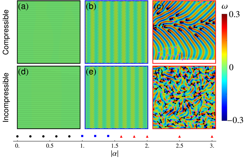
Figure 1 shows typical configurations of active nematics in compressible versus incompressible flows, starting from a homogeneous ordered state and increasing activity. At low activity, the homogeneous state remains stable, for both compressible and incompressible systems (Figs. 1a and 1d), due to the presence of substrate friction. Increasing activity destabilizes the homogeneous state, giving rise to a bend pattern (for ) in the director field (Figs. 1b, 1e, and Movies 1 and 2). The instability threshold is the same for both compressible and incompressible systems and is consistent with the value obtained from linear stability analysis Srivastava et al. (2016), which predicts a critical activity . At higher activity, however, relaxing the incompressibility constraint changes fundamentally the character of the defect patterns. Incompressible systems transition to a state of defect chaos (Fig. 1f and Movie 4), with proliferation of half-integer defects in the nematic texture and spatio-temporal chaotic vortical flows, as observed in many previous studies Giomi et al. (2014); Doostmohammadi et al. (2018). When the flow is compressible defect pairs also unbind at high activity. However, instead of the familiar chaotic dynamics, we observe a well-organized structure, consisting of a smectic-like state of equally spaced Néel or kink walls that have been referred to as arches due to the structure of the director field (Fig. 1c) Patelli et al. (2019), with associated polar order of defects. Upon nucleation of defect pairs, the defects move away from their companions, leaving a kink-wall structure of the director field in their wake. Active torques align the defect and the kink walls, resulting in polar flocking of the defects. This ordered state of defect and nematic texture was found to be a stable solution of the hydrodynamic of a defect gas derived in Ref. Shankar and Marchetti (2019). These structures have been previously found to be stable in continuum simulation of dry active nematics DeCamp et al. (2015); Putzig et al. (2016), but seemed to be long-lived metastable states in particle simulations of the same system Patelli et al. (2019). They are also similar to the filamentous network of domain walls that was recently shown to dominate the coarsening dynamics of polar active matter Chardac et al. (2021). In our compressible dry nematic, however, arches form a stable ordered state.
IV Arch patterns and stability
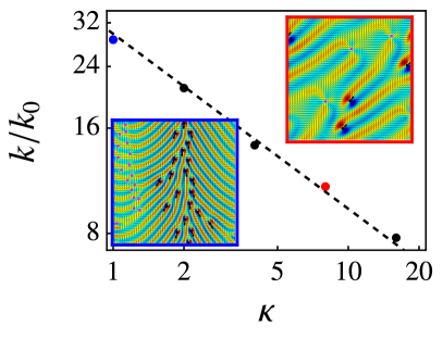
To quantify the periodicity of arches, we Fourier transform the phase field obtained from numerical simulations in the regime where arches coexist with topological defects. The peak of the Fourier spectrum allows us to extract a characteristic wavenumber of the arch pattern, and the results show that , where . Figure 2 shows as a function on a log-log scale at a fixed activity , demonstrating that indeed .
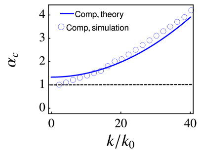
To examine the stability of uniform arches in compressible flows, we solve numerically Eqs. (1) and (4) with an initial condition given by an arbitrary number of perfectly aligned arches. Specifically, we set and impose an initial texture (mod ), with an integer representing the number of equilibrium arches that can be accommodated in a system of size . Figure 3 shows the critical activity as function of the number of initial arches and above which the initial uniform arch pattern becomes unstable to defect nucleation. We notice that increases monotonically with the initial arch wavenumber implying that the transition to the regime of coexistence between arches and orientational defects depends on initial conditions, thus the metastability of arches. The numerical protocol of destabilizing initially uniform arches is done in the absence of any noise and by gradually increasing activity. In this case, arches remain metastable also for . However, any additional noise perturbations will melt the arches into the uniform ordered state as shown in the state diagram in Fig. (1). This is not the case for where many possible arch states can be stable as discussed next.
By a theoretical stability analysis, we can also further understand the role of flow compressibility in stabilizing arch patterns. To do this, it is convenient to write Eqs. (1) and (4) in complex coordinates by introducing , , , and . The Q-tensor and flow velocity are written equivalently as complex scalar fields, and . In this notation, Eqs. (1) and (4) take the form
| (5) |
and
| (6) |
The incompressibility constraint reads . The first two terms on the right hand side of Eq. (5) are the convective terms, which are followed by the terms for vorticity.
When the flow is compressible, the pressure gradients vanishes and the flow velocity can be eliminated from the evolution. We seek a steady-state solution for perfectly aligned arches
| (7) |
where is a complex amplitude. In this case, the advective term and the term coupling to vorticity cancel each other, such that we obtain an equation for as
| (8) | ||||
This equation has a nontrivial steady-state solution given by
| (9) |
where
| (10) |
For , vanishes and this reduces to the homogeneous nematics.
To examine the stability of this arch solution against linear perturbations, we let
| (11) |
and linearize Eqs. (1) and (4) in , leading to
| (12) | ||||
Since Eq. (12) is a linear differential equation with -dependent coefficients, Fourier modes with different wavenumbers along are generally coupled and the eigenfunctions are not plane waves. One approach would then be to truncate the Fourier expansion to some order and numerically diagonalize the operator on the right hand side of Eq. (12), as done for instance in Ref. Jiang and Wang (2019). For the purpose of determining the critical activity, we find it suffices, however, to retain only the wavenumber that sets the periodicity of the arch solution and write
| (13) |
Substituting Eq. (13) into Eq. (12) and keeping only the lowest order mode in , we find that, given is real, the dynamical equations for , , and is block diagonal. The problem of finding the relaxation rate then reduces to the solution of two coupled equations that can be written as
| (14) |
where
| (15) |
The eigenvalues of the dynamical matrix are and correspond to the growth rates of the two modes. The instability is controlled by the largest growth rate , given by
| (16) |
Arches are therefore unstable for magnitudes of activity larger than the critical value
| (17) |
where the coefficient of changes sign. The wavenumber of the most rapidly growing mode vanishes at the onset of instability.
The analytically-predicted dependence of on the arches wavenumber is shown as a solid blue line in Fig. 3 and compares well with the results of numerical simulations.
V Defect ordering
To quantify orientational order of defects, we define the polarization of the -th defect as Vromans and Giomi (2016); Tang and Selinger (2017). In the compressible fluid, we measure a vector global polar order parameter of the defects as an ensemble average of the defect polarizations given by
| (18) |
where is the number of defects in the system at time . To quantify the correlation between arches and polar order of defects, we additionally measure the mean (spatially-averaged) phase gradient
| (19) |
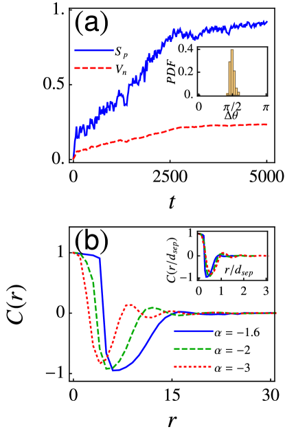
as a global indicator of the arches periodicity. Figure 4(a) shows that the magnitudes of both these measures increase in time in a correlated manner, and both saturates to a constant value on similar time scales. The inset is the histogram of the angle between and and is strongly peaked at , demonstrating that the polar defect order is normal to the arches periodicity. These findings are consistent with the hydrodynamic theory presented in Ref. Shankar and Marchetti (2019).
In an incompressible fluid, defects do not reveal global order, but may exhibit local order, as previously reported in Ref. Pearce et al. (2021), and which is extracted from the radial dependence of the defect orientation correlation function on the distance between defects
| (20) |
where is the total number of defect pairs with separation within . Figure 4(b) shows the correlation function for various values of activity . has a pronounced dip at small distances, signifying local nematic defect order. Furthermore, when the distance is scaled by the average defect separation , for different values of activity nearly collapse into a single curve (inset of Fig. 4(b)). Our findings on local nematic defect order are consistent with those reported in Ref. Pearce et al. (2021) for an incompressible active fluid with no substrate friction.
VI Conclusions
We have examined numerically and analytically the emergent dynamics of two-dimensional active nematics on a substrate with compressible and incompressible fluid flow. We find that long-range constraints imposed by incompressibility has a profound influence of the spontaneous flow structures observed upon increasing activity. While incompressible systems transition from a stationary homogeneous state to chaotic spatiotemporal dynamics with proliferation of unbound nematic defect pairs, compressible ones organize in a smectic-like state of aligned arches in the nematic texture and associated polar order of defects. We demonstrate explictely that arch patterns are stable in the compressible case below an arch-width dependent critical activity, which we calculate analytically. These arches underlie defect ordered states previously reported in compressible fluids that incorporate density fluctuations Putzig et al. (2016); Patelli et al. (2019).
To put our results in context, we briefly compare them to previous work. Polar order of defect and associated smectic arrangement of arches has been reported previously in simulations of hard spherocylinders DeCamp et al. (2015) and in numerical solution of the continuum hydrodynamics of dry active nematic both in the “compressible” limit implemented here Srivastava et al. (2016), as well as for a truly incompressible fluid with conserved density allowed to fluctuate Putzig et al. (2016). Oza and Dunkel Oza and Dunkel (2016) also used a dry continuum model, but placed themselves directly in the unstable regime and neglected entirely the rotational effects of the flow. In this limit they observed a variety of ordered structures, including defect lattices and anti-polar order of defects. Due to these differences in the model, a direct comparison with other results is not straightforward. Arches and associated polar defect order have also been observed in numerical simulations of Viscek-like model of self-propelled point particles that periodically reverse their direction of motion and interact through both aligning and repulsive interactions Patelli et al. (2019). Arches solutions where, however, found to be metastable in an associated continuum formulation of the same model, and no defect order was obtained in the continuum model.
Simulations of incompressible wet active nematics where dissipation is controlled entirely by viscous stresses have revealed local antialignment of defects, but no longer range order Pearce et al. (2021), as we find here in the dry limit. Finally, Nejad et al. Nejad et al. (2021) have recently examined the interplay between viscous and frictional dissipation in incompressible fluids. At large friction they observe arches and local polar defect order, but this behavior seems to be transient. In fact we have also observed such structures in the incompressible case, but they are never present in the long-time steady state, consistent with our analytical results on arches solutions. A more detailed comparison with their work is, however, not possible since these authors use the shear viscosity, which is zero in our work, to determine the units of time. Additionally, their large friction limit can also be interpreted as the limit of very low activity. It is therefore not surprising that in these limit they find no defect proliferation.
Our work demonstrates that nematic texture and defect order in active liquid crystals depend strongly on the nature of the flows. It further identifies the origin of apparent discrepancies reported in the literature on polar or nematic order of defects as arising from the constraint imposed by incompressibility.
Finally, it may be possible to observe the smectic arch state and polar defect order in dense, possibly jammed active systems where friction is the primary dissipation mechanism. In fact experiments in dense monolayer of spindle-shaped cells have revealed structures that resemble arches at high cell density, where the the cells are essentially jammed and defects are no longer motile Duclos et al. (2017). The phenomena described here may also be relevant to bacterial colonies growing on a frictional substrate.
Acknowledgements.
This work was supported by the National Science Foundation Grants No. DMR-2041459 (Z.Y. and M.C.M.) and No. PHY-1748958 (S.P, Z.C. and M.J.B.).References
- Doostmohammadi et al. (2018) A. Doostmohammadi, J. Ignés-Mullol, J. M. Yeomans, and F. Sagués, Nature communications 9, 1 (2018).
- Sanchez et al. (2012) T. Sanchez, D. T. Chen, S. J. DeCamp, M. Heymann, and Z. Dogic, Nature 491, 431 (2012).
- Zhang et al. (2018) R. Zhang, N. Kumar, J. L. Ross, M. L. Gardel, and J. J. De Pablo, Proceedings of the National Academy of Sciences 115, E124 (2018).
- Thutupalli et al. (2015) S. Thutupalli, M. Sun, F. Bunyak, K. Palaniappan, and J. W. Shaevitz, Journal of The Royal Society Interface 12, 20150049 (2015).
- Doostmohammadi et al. (2016a) A. Doostmohammadi, S. P. Thampi, and J. M. Yeomans, Physical review letters 117, 048102 (2016a).
- Duclos et al. (2017) G. Duclos, C. Erlenkämper, J.-F. Joanny, and P. Silberzan, Nature Physics 13, 58 (2017).
- Blanch-Mercader et al. (2018) C. Blanch-Mercader, V. Yashunsky, S. Garcia, G. Duclos, L. Giomi, and P. Silberzan, Physical review letters 120, 208101 (2018).
- Alert et al. (2022) R. Alert, J. Casademunt, and J.-F. Joanny, Annual Review of Condensed Matter Physics 13 (2022).
- Giomi et al. (2013) L. Giomi, M. J. Bowick, X. Ma, and M. C. Marchetti, Physical review letters 110, 228101 (2013).
- Pismen (2013) L. M. Pismen, Physical Review E 88, 050502(R) (2013).
- Giomi et al. (2014) L. Giomi, M. J. Bowick, P. Mishra, R. Sknepnek, and M. Cristina Marchetti, Philosophical Transactions of the Royal Society A: Mathematical, Physical and Engineering Sciences 372, 20130365 (2014).
- Keber et al. (2014) F. C. Keber, E. Loiseau, T. Sanchez, S. J. DeCamp, L. Giomi, M. J. Bowick, M. C. Marchetti, Z. Dogic, and A. R. Bausch, Science 345, 1135 (2014).
- Kawaguchi et al. (2017) K. Kawaguchi, R. Kageyama, and M. Sano, Nature 545, 327 (2017).
- Saw et al. (2017) T. B. Saw, A. Doostmohammadi, V. Nier, L. Kocgozlu, S. Thampi, Y. Toyama, P. Marcq, C. T. Lim, J. M. Yeomans, and B. Ladoux, Nature 544, 212 (2017).
- Maroudas-Sacks et al. (2021) Y. Maroudas-Sacks, L. Garion, L. Shani-Zerbib, A. Livshits, E. Braun, and K. Keren, Nature Physics 17, 251 (2021).
- Copenhagen et al. (2021) K. Copenhagen, R. Alert, N. S. Wingreen, and J. W. Shaevitz, Nature Physics 17, 211 (2021).
- Doostmohammadi et al. (2016b) A. Doostmohammadi, M. F. Adamer, S. P. Thampi, and J. M. Yeomans, Nature communications 7, 1 (2016b).
- Chaté (2020) H. Chaté, Annual Review of Condensed Matter Physics 11, 189 (2020).
- Simha and Ramaswamy (2002) R. A. Simha and S. Ramaswamy, Physical review letters 89, 058101 (2002).
- Srivastava et al. (2016) P. Srivastava, P. Mishra, and M. C. Marchetti, Soft matter 12, 8214 (2016).
- Putzig et al. (2016) E. Putzig, G. S. Redner, A. Baskaran, and A. Baskaran, Soft matter 12, 3854 (2016).
- Patelli et al. (2019) A. Patelli, I. Djafer-Cherif, I. S. Aranson, E. Bertin, and H. Chaté, Physical review letters 123, 258001 (2019).
- Shankar and Marchetti (2019) S. Shankar and M. C. Marchetti, Physical Review X 9, 041047 (2019).
- Beris et al. (1994) A. N. Beris, B. J. Edwards, et al., Thermodynamics of flowing systems: with internal microstructure, 36 (Oxford University Press on Demand, 1994).
- Marenduzzo et al. (2007) D. Marenduzzo, E. Orlandini, and J. M. Yeomans, Physical review letters 98, 118102 (2007).
- Giomi et al. (2010) L. Giomi, T. B. Liverpool, and M. C. Marchetti, Physical Review E 81, 051908 (2010).
- Oza and Dunkel (2016) A. U. Oza and J. Dunkel, New Journal of Physics 18, 093006 (2016).
- Shankar et al. (2018) S. Shankar, S. Ramaswamy, M. C. Marchetti, and M. J. Bowick, Physical review letters 121, 108002 (2018).
- DeCamp et al. (2015) S. J. DeCamp, G. S. Redner, A. Baskaran, M. F. Hagan, and Z. Dogic, Nature materials 14, 1110 (2015).
- Chung (2010) T. Chung, Computational Fluid Dynamics (Cambridge University Press, 2010).
- Chardac et al. (2021) A. Chardac, L. A. Hoffmann, Y. Poupart, L. Giomi, and D. Bartolo, Physical Review X 11, 031069 (2021).
- Jiang and Wang (2019) H. Jiang and S. Wang, Physical Review Research 1, 033164 (2019).
- Vromans and Giomi (2016) A. J. Vromans and L. Giomi, Soft matter 12, 6490 (2016).
- Tang and Selinger (2017) X. Tang and J. V. Selinger, Soft matter 13, 5481 (2017).
- Pearce et al. (2021) D. J. G. Pearce, J. Nambisan, P. W. Ellis, A. Fernandez-Nieves, and L. Giomi, Physical Review Letters 127, 197801 (2021).
- Nejad et al. (2021) M. R. Nejad, A. Doostmohammadi, and J. M. Yeomans, Soft Matter 17, 2500 (2021).
Appendix A Linear stability analysis with elastic stress
We present in this section the linear stability analysis of the uniform nematic state with and , where . We omit the phenomenological surface tension term in this analysis and include a passive elastic stress
| (21) |
in the equation of the flow field. This analysis demonstrates that, in the linearized theory, the phenomenological surface tension term in the main text captures some of the effects of the passive elastic stress. Appendix C provides a more general derivation of the surface tension term from elastic stress in a compressible fluid.
The linearized equation of motion of the order parameter is given by
| (22) |
where
| (23) |
A.1 Incompressible fluid
In an incompressible flow, the linearized equations of the flow are
| (24) | ||||
where is the active stress and is the passive elastic stress. The flow field can be solved in Fourier space as
| (25) |
where the transverse projection operator is .
The components of the active contribution to the strain rate tensor are
| (26) | ||||
and
| (27) | ||||
In the above equations, we have introduced , and , so that , , . The active contribution to the flow vorticity is
| (28) | ||||
The components of the passive contribution to the strain rate tensor are
| (29) | ||||
and
| (30) | ||||
The passive contribution to the vorticity is
| (31) | ||||
We see that the passive parts of the strain rate tensor and vorticity contain terms proportional to , which is an effective surface tension term.
Collecting the above results into Eq.(A2) then gives an explicit expression of the dynamical matrix for . One can check that the most unstable mode in an extensile active nematic system is the pure bend mode, corresponding to Srivastava et al. (2016). In this case, the dynamics of and are decoupled as
| (32) | ||||
is unstable if . The term provides stability at short length scale.
A.2 Compressible fluid
In a compressible fluid, the linearized equations of the flow are
| (33) |
The active and passive contributions to the flow vorticity remain the same as in Eq.(A8) and Eq.(A11). The active part of the strain rate tensor is given by
| (34) |
The components of the passive contribution to the strain rate tensor are given by
| (35) |
and
| (36) |
Similarly to before, the stability of can be analyzed by substituting these results into Eq.(A2). The most unstable mode in a compressible fluid is also the pure bend mode, in which case, the dynamics of is given by
| (37) | ||||
The critical activity for instability is the same as the one in the incompressible case.
Appendix B Absence of arch solution in incompressible fluids
In this appendix we recall the existence of arch solution in a compressible system and detail its absence for incompressible flows. We start with the equations in complex coordinates, as given in Eqs. (5) and (6), with the incompressibility constraint . The first two terms on the right hand side of Eq. (5) are the convective terms, which are followed by the terms for vorticity.
In the case of compressible flow the pressure gradient on the right hand side of Eq. (6) vanishes and one can immediately eliminate the flow velocity from Eq. (5) using . Substituting in Eq. (5) the solution for perfectly aligned arches with a constant phase gradient in the form given in Eq. (7), we then obtain Eq. (8), where the advective term and those coupling to vorticity exactly cancel. The resulting equation can then be solved in a steady state, leading to the value of given in Eq. (9).
The same arch structure is not a solution for the case of incompressible flow because in this case the nonlinear advective term and the term coupling to vorticity do not cancel. To see this, we solve for the pressure gradient in Eq.(4), with the result
| (38) |
where we assume the Q tensor is independent of , and is a real harmonic function. The superscript denotes a vector transpose. The flow is then given by
| (39) | ||||
where the second line represents the flow in complex coordinates. Using the ansatz in Eq.(7), the advective terms yield
| (40) |
and
| (41) | ||||
In other words the contribution from the coupling to vorticity is no longer balanced by advection. The above equation cannot be satisfied by a harmonic function . A solution would require, for instance, which would give Therefore, the arch ansatz with constant phase gradient is not a steady state solution when the flow is incompressible.
We note that in Ref. Nejad et al. (2021) by focusing on the dynamics of the phase field and assuming constant order parameter magnitude, the authors showed that the vorticity terms can be balanced by the elastic stiffness term at low activity, , allowing arches solutions with spatially varying phase gradient.
Appendix C Effective surface tension
Here we show that the effective surface tension arises from the elastic stress defined by Eq. (21) due to nematic distortions, namely
The overdamped flow velocity induced by this is therefore
and contributes to the flow alignment of tensor from Eq. (1) through an additional strain given by
where
From the symmetry of the tensor, it quickly follows that this elastic strain is proportional to . Consequently, the flow alignment due to this strain reduces to an effective surface tension. To see this, we evaluate the -component of which is given by
Similarly, it follows that
where . The term is
Thus, to this leading order, the surface tension reduces to . In general, however, it can also be taken as an independent parameter, and this is the route considered here.