Auditing Visualizations: Transparency Methods Struggle to Detect Anomalous Behavior

Abstract

Model visualizations provide information that outputs alone might miss. But can we trust that model visualizations reflect model behavior? For instance, can they diagnose abnormal behavior such as planted backdoors or overregularization? To evaluate visualization methods, we test whether they assign different visualizations to anomalously trained models and normal models. We find that while existing methods can detect models with starkly anomalous behavior, they struggle to identify more subtle anomalies. Moreover, they often fail to recognize the inputs that induce anomalous behavior, e.g. images containing a spurious cue. These results reveal blind spots and limitations of some popular model visualizations. By introducing a novel evaluation framework for visualizations, our work paves the way for developing more reliable model transparency methods in the future.

1 Introduction

Neural networks with similar validation accuracy can behave very differently when deployed. A network can have a high validation accuracy, but be vulnerable to distribution shift, backdoors, or spurious cues learned during training. To diagnose these failures, model visualizations rely on the internals of a network, such as the activations of inner layers or the model’s gradients (Molnar, 2022). By opening the black box, they may better uncover failure modes (Hernandez et al., 2022), tell us where to intervene to repair models (Wong et al., 2021; Santurkar et al., 2021), or provide auxiliary training objectives (Koh et al., 2020).

However, model visualizations can only fulfill these promises if they actually track model behavior. Previous evaluations have shown that many visualization methods fail basic tests of validity (Adebayo et al., 2018, 2020). However, we seek more than simply pointing out failures in methods: we would like a quantifiable goal for interpretability methods to aspire to.

Following Adebayo et al. (2020), we focus on the goal of debugging model errors: we say that a method is good at debugging if it can successfully uncover a wide range of possible anomalous behaviors in models. To measure this, we train a wide variety of models with anomalous behaviors, such as models containing backdoors or trained with spurious cues. We also train a set of reference models, that do not exhibit anomalous behavior, and we test whether visualization methods behave differently on the reference and anomalous models.

Our pipeline for evaluating visualizations is illustrated in Figure 1. We leverage the fact that visualizations are images and thus can be embedded in a semantic feature space. Under our evaluation metric, a visualization method distinguishes anomalous models if its embedding for the anomalous model is far from the reference models, relative to the variation within the reference models. We use this metric to measure whether visualizations can (1) detect that a network is anomalous, and (2) determine how the model is unusual, i.e. localize the inputs where it behaves atypically.

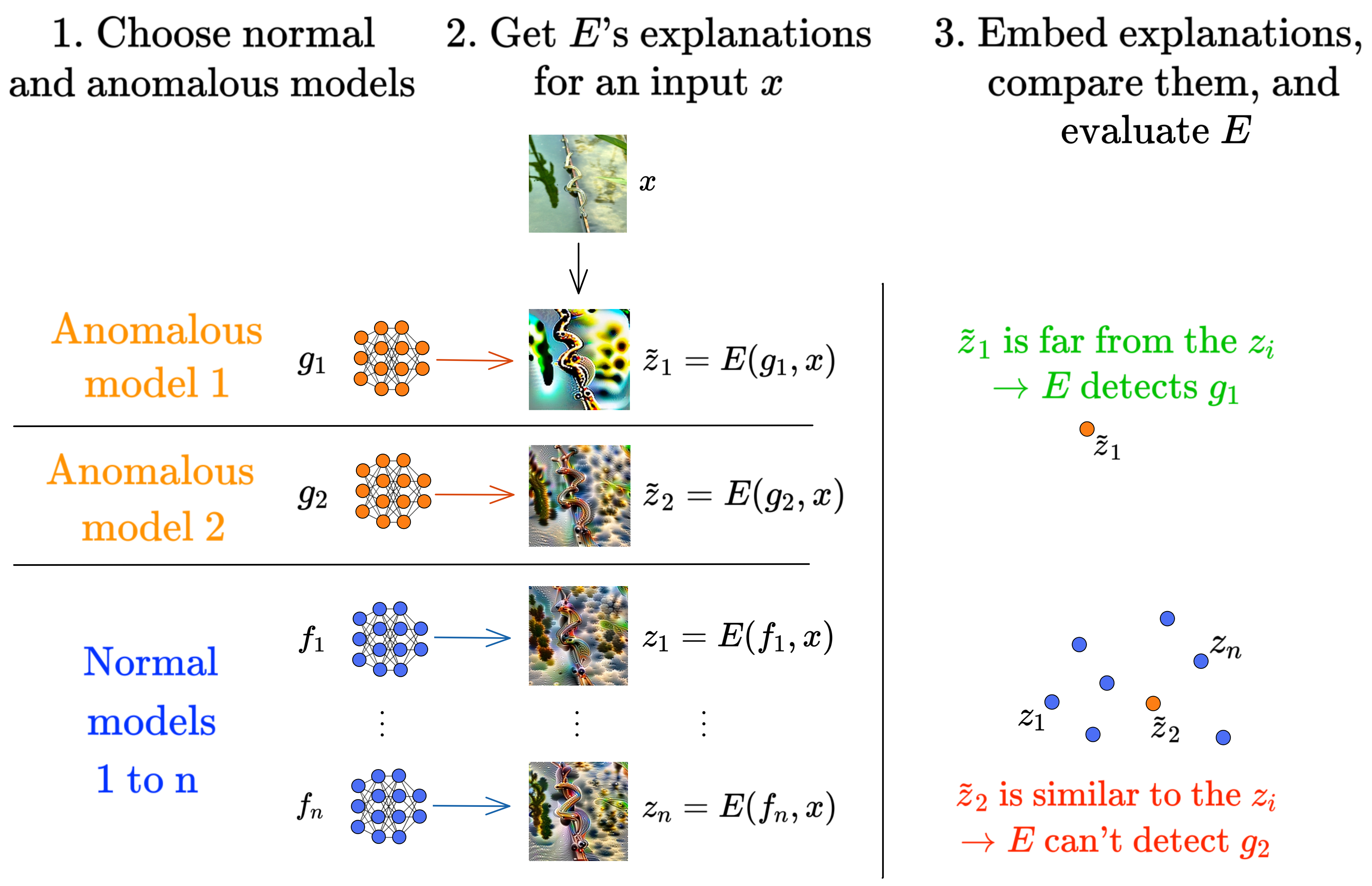
Figure 1: Testing whether a method $E$ can detect if a model is anomalous (Section 4). Here $E$ can detect that $g_{1}$ is anomalous, but not $g_{2}$.

We evaluate five widely used model visualization techniques: Caricatures (Olah, 2018), Integrated Gradients (Sundararajan et al., 2017), Guided Backpropagation (Springenberg et al., 2015), Grad-CAM, and Guided Grad-CAM (Selvaraju et al., 2019). For each technique, we test whether it can detect 24 anomalous models across 7 categories: adversarial training (Madry et al., 2019), randomized smoothing (Cohen et al., 2019), shape bias (Geirhos et al., 2019), backdoors (Li et al., 2021), spurious features, training without data from certain classes, and training on a face-obfuscated version of ImageNet (Yang et al., 2021).

Our main takeaway is that model visualizations fail to detect and localize a large number of anomalies. Most methods only consistently detect anomalous models in the regime where the validation accuracy itself is lower than normal (stark anomalies, such as adversarial training), and struggle with anomalies that affect behavior on a smaller number of inputs (subtle anomalies, for example removing all the images in a single class from the training data). Moreover, methods often fail to localize the inputs for which behavior is different, such as images containing a spurious cue for the spurious features anomaly.

Taken together, our results underscore the need to systematically evaluate visualization methods to check that they track model behavior. If we view visualization methods as a way of auditing models, our detection and localization benchmarks are a form of counterauditing—planting intentionally corrupted models to check that they are discovered. To achieve high reliability in machine learning, such counteraudits are a crucial counterpart to regular audits. Our framework can easily be adapted to other visualization methods and anomalies, and we encourage the community to use such evaluations in the future.

2 Related Work

Our work is closely related to Adebayo et al. (2018) and Adebayo et al. (2020), which evaluate feature attribution methods by their ability to diagnose different kinds of model errors. Similarly, Zhou et al. (2021) and Bastings et al. (2021) study whether feature attributions detect spurious features, and Adebayo et al. (2022) shows that model explanations can’t uncover unknown spurious correlations. Compared to these works, our evaluation framework is more flexible: given a set of reference models and a distance metric between model visualizations, it can work for any visualization method, model anomaly, and any modality (vision, language, or other). This flexibility allows us to consider a much greater variety of model anomalies (24 anomalous models), which provides more detailed information about the limitations of visualization methods. It also makes it possible to compare feature attributions and different kinds of methods, such as feature visualizations.

Lin et al. (2020) study whether 7 feature attribution methods, including Guided Backpropagation, are able to localize backdoor triggers: unlike us, they find that most methods fail, however they consider more sophisticated trojan attacks. Following our work, Casper et al. (2023) also used trojan discovery to benchmark feature attributions and feature synthesis methods, and found that most feature attribution methods could approximately locate the trigger, although failed to beat a simple baseline (see Figure 2 in (Casper et al., 2023). In contrast with these works, we consider anomalies other than backdoors, we define localization in a different and more general way, and we also assess whether a method can detect that a model is anomalous.

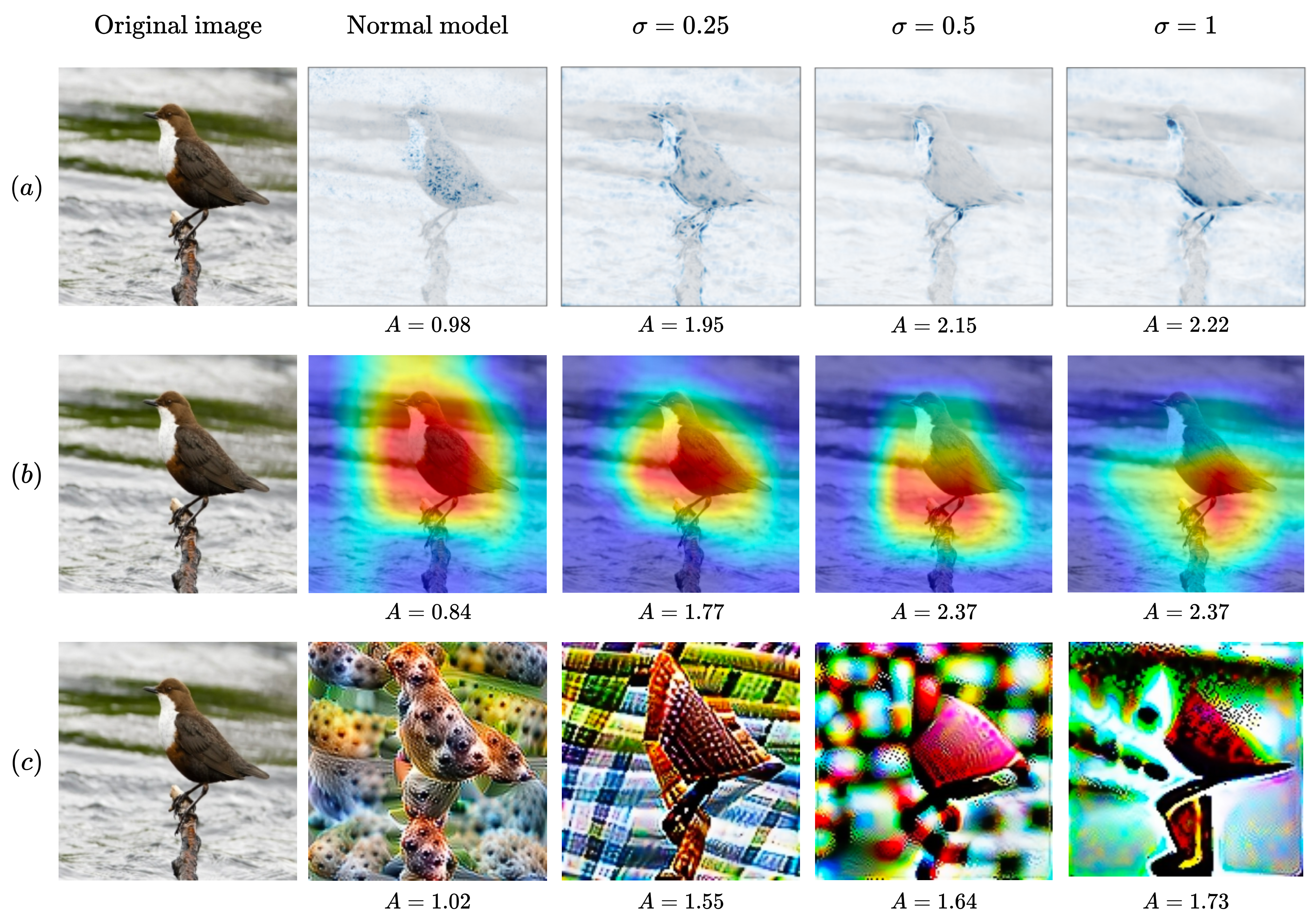
Figure 2: All methods are able to detect stark anomalies such as randomized smoothing (adding Gaussian noise to training inputs). We show model explanations by (a) Integrated Gradients, (b) Grad-CAM, and (c) Caricatures (layer (3,2,2)). We consider a normal model and anomalous models trained with increasing amounts $\sigma$ of randomized smoothing. The explanations of the anomalous models appear very different from those of the normal model, and their anomaly scores $A$ are greater.

Ding et al. (2021) apply a similar framework to evaluate representation similarity metrics: just like the model visualizations of an anomalous model should be different from those of a normal model, a representation similarity metric should assign a high distance between representations with different functional properties.

Finally, there are other approaches to ground and evaluate transparency methods. One especially ambitious goal is to reverse engineer entire parts of neural networks: a preliminary example is Cammarata et al. (2021), in which the authors use feature visualization methods to hand-code a curve detection module in InceptionV1. A related perspective is model repair: for example, Wong et al. (2021) and Singla & Feizi (2021) both introduce new visualization-based methods to help humans identify and repair spurious features in models. Finally, another way of evaluating transparency methods is to run human subject studies to determine how much they help humans understand the underlying models Doshi-Velez & Kim (2017); Bhatt et al. (2020).

3 Problem Setup

In this section, we first introduce the anomalous models and reference models used in our evaluations (Section 3.1), then define model visualizations and visualization anomaly scores (Section 3.2). Finally, we introduce the transparency methods considered in this work (Section 3.3).

3.1 Anomalous models and reference models

We call a model $f$ anomalous if it differs from a set of reference models that specify normal behavior, for example in its accuracy on an out-of-distribution test set.

Reference models. In what follows, all the models we consider will be ResNet-50 variants, and our reference models will be $n=12$ ResNet-50 networks $g_{1},\dots,g_{n}$ trained on ImageNet with the same hyperparameters but different random seeds.

Anomalous models. For the choice of the anomalous model $f$, we consider 24 ResNet-50 models comprising 7 different types of anomalies. The first three families of anomalies are stark (they always induce a significant drop in validation accuracy), while the remainder are subtle (their behavior is only different on out-of-distribution data). We will often find that model visualizations can detect stark anomalies, but not the subtle ones. We describe each family below, with full training details given in Section A.2.

Randomized Smoothing: These models are trained on ImageNet images perturbed by isotropic Gaussian noise with standard deviation $\sigma$, for $\sigma\in\{0.25,0.5,1.0\}$. We obtained checkpoints from the ImageNet Testbed (Taori et al., 2020). Randomized smoothing substantially decreases the test set accuracy, to at most $0.4$ for $\sigma=0.25$. Unlike in applications to adversarial robustness, we do not add noise to the inputs at evaluation time.

Adversarial Training: These are robust models adversarially trained on ImageNet with a PGD adversary. We obtained models with $\ell^{\infty}$-norm constraints of $\epsilon=4$ and $8$ from Engstrom et al. (2019a), and models with $\ell^{2}$-norm constraints of $\epsilon=0.01$, $0.1$, $1$, and $5$ from Salman et al. (2020). Most of these models exhibit a noticeable drop in validation accuracy.

Shape Bias: This anomalous model is trained on Stylized-ImageNet (Geirhos et al., 2019), which makes it more sensitive to shapes and less sensitive to textures when classifying images. Once again, the resulting model has low accuracy on the ImageNet validation set ($0.602$).

Spurious Features: We trained models on ImageNet, but where a fraction $\delta$ of each training batch’s images had the class index overlaid at the bottom right of the image. We trained 4 such models with $\delta\in\{1.0,0.5,0.3,0.1\}$. The spurious features have a large impact on validation accuracy when $\delta=1.0$, but the effect nearly disappears for smaller $\delta$.

Backdoors: We trained 6 backdoored ResNets with a pixel-modification data poisoning attack by following the methodology in Bagdasaryan & Shmatikov (2021). These models exhibit a negligible drop in validation accuracy (at most $0.01$ and sometimes smaller). On the other hand, their out-of-distribution accuracy on images with the backdoor trigger is near zero.

Removing data from a class: We trained networks on variants of ImageNet with all images from a given class removed. We considered 3 such models, removing data from classes 414 (backpack), 400 (academic gown), and 218 (Welsh springer spaniel). We sampled classes 400 and 414 uniformly from the 1000 classes. Because ImageNet contains so many dogs, we thought that removing data from a dog class would be harder to detect, so we chose class 218 by sampling uniformly from dog classes. These anomalies have a negligible effect on the overall validation accuracy, but drop the accuracy on the missing class to 0.

Training on blurred images: Finally, we trained a model on a variant of ImageNet with blurred faces (Yang et al., 2021). This decreases the validation accuracy by less than $1\%$, but has a large effect on some classes, such as harmonica, where key information becomes blurred.

Table 1: Fraction of anomalous models detected by each method. All methods succeed at the detection task for the stark anomalies, but fail for most of the subtle anomalies.

	Stark Anomalies				Subtle Anomalies
Anomaly Type	Smoothing	Shape Bias	Adv. ($\ell^{\infty}$)	Adv. ($\ell^{2}$)	Backdoor	Spurious	Blur	Missing
GBP	1	1	1	0.75	0.67	0.5	0	0
IG	1	1	1	1	0.17	1	0	0
GC	1	1	1	0.75	0.5	0.25	0	0
GGC	1	1	1	0.75	0.5	0.25	0	0
Caricatures	1	1	1	1	1	0.25	0	0

3.2 Anomaly scores for visualizations

Recall that model visualizations $E(\cdot,\cdot)$ are functions that take as arguments a neural network $f$ and input $x$, and output some information $E(f,x)$ about how $f$ processes $x$. This information is usually a vector or tensor, e.g. an image in the case of feature visualizations.

We will call an visualization $z=E(f,x)$ anomalous when it is far away from reference visualizations $z_{i}=E(g_{i},x)$. Given a metric $\mathrm{d}(\cdot,\cdot)$ between visualizations, a simple way to quantify this is via the average distance between $z$ and the reference visualizations, normalized by the average distance between the reference visualizations themselves:

$$A(f,E,x)\mathrel{\mathop{:}}=\frac{\frac{1}{n}\sum\limits_{i=1}^{n}\mathrm{d}(z,z_{i})}{\frac{2}{n(n-1)}\sum\limits_{1\leq i<j\leq n}\mathrm{d}(z_{i},z_{j})}.$$ (1)

We call this ratio the anomaly score of $z$ compared to the reference visualizations $z_{1},\dots,z_{n}$. When this ratio is much larger than 1, then the visualization $z=E(f,x)$ is anomalous. A good transparency method should assign a high anomaly score to models with anomalous behavior.

For the metric $\mathrm{d}(\cdot,\cdot)$, we use the LPIPS distance, since Zhang et al. (2018) show that it aligns well with human perceptual similarity. In the main text, we used AlexNet features for the LPIPS distance, because Zhang et al. (2018) found that they perform the best. As a robustness check, we also computed anomaly scores for LPIPS distances with two other networks, VGG and SqueezeNet; we show the corresponding results in the Appendix.

3.3 Visualization methods

We assess four feature attribution methods and one feature visualization method.

Feature attributions. Consider a neural network classifier $f:\mathbb{R}^{d}\to\mathbb{R}^{C}$, which outputs a logit for each possible class $1\leq c\leq C$. For an input $x$, a feature attribution of $f$ with target class $c$ is a tensor with the same shape as $x$. Intuitively, it represents the relevance of each of $x$’s entries to $f(x)$’s output logit for class $c$. In what follows, we’ll always take $c$ to be the output class $c_{\text{max}}=\underset{c}{\text{argmax}}f_{c}(x)$. We consider four feature attribution methods:

Guided Backpropagation (GBP) (Springenberg et al., 2015) takes the gradient $\nabla_{x}f_{c}(x)$ of the output logit with respect to the pixels, and modifies it by only backpropagating non-negative gradients through ReLU nonlinearities.

Integrated Gradient (IG) (Sundararajan et al., 2017) attributions take the integral of the gradient of $f_{c}$ along a linear path connecting $x$ to some base point $x_{0}$:

$$\left(x-x_{0}\right)\times\int_{0}^{1}\nabla_{x}f_{c}\left(x_{0}+\alpha\left(x_{i}-x_{0}\right)\right)d\alpha.$$ (2)

Grad-CAM (GC) (Selvaraju et al., 2019) highlights large regions of the input image that are important for the prediction. It is the sum of the activations of the final convolutional layer’s feature maps, weighted by the gradient of $f_{c}$ with respect to each feature map.

Guided Grad-CAM (GGC) (Selvaraju et al., 2019) takes the product of guided backpropagation attributions and GradCAM attributions.

We obtained Guided Backpropagation, Integrated Gradients and Guided Grad-CAM attributions using the Captum library (Kokhlikyan et al., 2020) with default settings. We obtained Grad-CAM attributions using the pytorch-grad-cam library (Gildenblat & contributors, 2021). We display these visualizations by superposing the attributions on top of the input image (c.f. the first two rows of Figure 2).

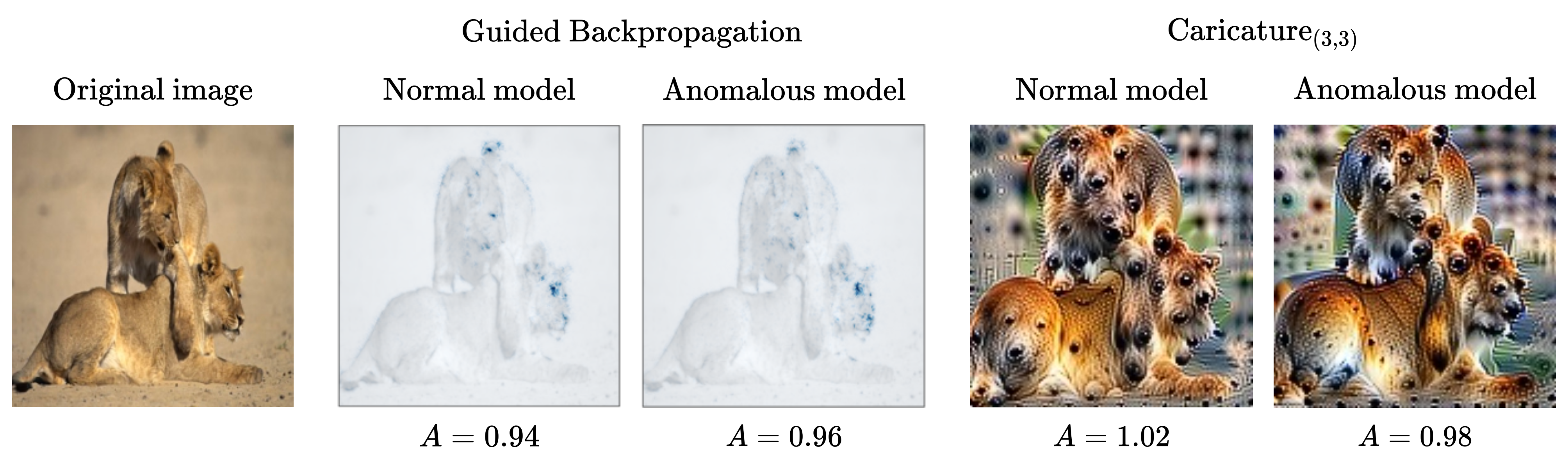
Figure 3: Most methods struggle to detect subtle anomalies like Spurious Features. We show model explanations by Guided Backpropagation and Caricatures (layer (3,3)) for a normal model and a Spurious Features model ($\delta=0.3$), with each explanation’s anomaly score $A$. Both methods fail to detect that the model is anomalous, and the explanations of both models appear very similar.

Feature Visualization: Caricatures. For a neural net classifier $f$, let $f_{\ell},1\leq\ell\leq L$ denote its layers, i.e. $f_{\ell}$ maps an input $x$ to the vector of activations at layer $\ell$. Intuitively, a Caricature describes what a layer “sees” in an input $x$ by visualizing the activation vector $f_{\ell}(x)$.

Formally, the Caricature of an input $x$ at layer $\ell$ is the solution to the following optimization problem (Olah, 2018): $\text{Caricature}_{\ell}(x,f):=\text{argmax}_{x^{\prime}}\langle f_{\ell}(x^{\prime}),f_{\ell}(x)\rangle$. In practice, $\text{Caricature}_{\ell}(x,f)$ solves a regularized, preconditioned, and data-augmented version of this optimization problem (see Olah et al., 2017, “The Enemy of Feature Visualization”). We obtained Caricatures (c.f. Figure 2c) by running 512 steps of optimization with the Lucent (Kiat, 2021) library’s default parameters.

4 Detection

In this section, we formally define our detection metric, then describe our experimental procedure. Finally, we present and interpret our empirical results.

Detection Metric. To test whether a method $E(\cdot,\cdot)$ can detect an anomalous model, we compute visualizations on a set of $m$ sample images $\{x_{1},\ldots,x_{m}\}$. We define the overall anomaly score of a model, $\bar{A}(f,E)$, as the average of the anomaly scores for the visualizations $E(f,x_{1}),\ldots,E(f,x_{m})$. We say that $E$ detects $f$ if $\bar{A}(f,E)$ is larger than all the normal models’ anomaly scores $\bar{A}(g_{i},E)$.

Experimental Procedure. We sampled $m=50$ input images uniformly from the ImageNet test set as our sample images $x_{j}$. To reduce computation time for Caricatures, we visualized a subset of $N_{\ell}=7$ layers in different parts of the model: layers (2,2,1), (3,0,3), (3,2,2), (3,3), (3,4,3), (4,0,3), and (4,3,2). We chose these layers to have information about different parts of the network: in earlier or later stages, in earlier or later residual blocks within a stage, and after or within residual blocks. For concision, we averaged the anomaly scores over these 7 layers as well as the 50 images to obtain an overall anomaly score for all caricatures $\bar{A}(f,\text{Caricatures})$. We show individual layer results in the Appendix. Integrated Gradients, Guided Backpropagation, Grad-CAM and Guided Grad-CAM do not depend on a layer: for them, we just average over images and report $\bar{A}(f,\text{IntGrad})$ and $\bar{A}(f,\text{GBP})$.

Results for stark anomalies. For every transparency method $E$ and every family of anomalous models, we report the fraction of anomalous models that $E$ detects in Table 1. The five methods are able to detect that all the models trained on Stylized ImageNet or with randomized smoothing are anomalous. They also usually detect that adversarially trained models are anomalous, although GBP, Grad-CAM, and Guided Grad-CAM fail to detect $\ell^{2}$-adversarial training with radius $\epsilon=0.01$.

Qualitatively inspecting the visualizations corroborates these results. Figure 2 shows the Integrated Gradients, Grad-CAM, and Caricature_(3,2,2) visualizations of the randomized smoothing models and a normal model. The visualizations of the anomalous models appear very different from those of the normal model. Moreover, they appear more different from the normal visualizations as $\sigma$ increases.

Results for subtle anomalies. The results are much worse for the subtle anomalies. No methods detect that any of the networks trained on blurred faces or with missing data are anomalous. For backdoors and spurious cues, the detection results differ between methods: for example, Caricatures detect that all backdoored models are anomalous but only a quarter of models in the Spurious Features category, whereas Integrated Gradients detect that all the models that rely on spurious features are anomalous but only 17$\%$ of backdoored models.

Table 2: Localization AUROC (%) for every anomaly and explanation method, with AUROCs higher than 70% bolded. Although feature attributions successfully localize the backdoors, no method can localize all of the anomalies, and visualizations often have close to random performance, with $54\%$ of AUROCs between 40% and 60%.

Category	Backdoor						Missing class			Spurious				Blur
Anomaly	0	1	2	3	4	5	218	400	414	0.1	0.3	0.5	1.0
GBP	100	100	100	100	100	100	69	43	58	72	77	80	69	87
IG	99	97	98	98	99	94	57	61	46	82	77	85	42	85
GC	98	99	95	98	99	97	81	58	59	53	55	53	53	76
GGC	99	100	96	100	100	100	74	40	58	51	70	64	57	79
Car(2,2,1)	37	40	50	45	52	50	38	45	67	57	48	57	52	28
Car(3,0,3)	47	54	54	53	50	60	62	52	51	49	54	40	51	65
Car(3,2,2)	56	53	56	52	55	50	60	61	41	50	52	51	49	66
Car(3,3)	51	56	59	60	71	68	56	47	62	57	55	46	53	82
Car(3,4,3)	57	59	52	58	71	63	53	58	57	42	43	46	39	53
Car(4,0,3)	64	80	67	48	77	72	66	32	46	52	54	46	77	59
Car(4,2,3)	84	90	91	93	82	69	51	46	50	55	51	52	64	73

Once again, qualitatively inspecting the visualizations confirms these findings. For example, Figure 3 shows visualizations by Guided Backpropagation and Caricature_(3,3) of a normal model and a Spurious Features model with $\delta=0.3$. Both methods fail to detect that this model is anomalous, and for both methods the visualizations of the two models appear very similar.

In summary, most methods succeed at detecting stark anomalies, but fail for most of the subtle anomalies. Grad-CAM and Guided Grad-CAM perform the same, and generally worse than Integrated Gradients, Guided Backpropagation, and Caricatures. We show in the Appendix that these results are robust with respect to the choice of the metric between visualizations (Section A.1.1).

5 Localization

Having studied transparency methods’ ability to detect that a model is anomalous, we now turn to the question of localization.

Localization Metric. Given an anomalous model $f$, we assess a method $E(\cdot,\cdot)$’s localization ability via the question: is the anomaly score $A(f,E,x)$ highest on the inputs $x$ where $f$’s behaviour is unusual? We will measure $E$’s ability to distinguish these inputs via AUROC. Concretely, we sample $p=40$ “normal” inputs (e.g. from the ImageNet validation set), and $p$ “abnormal” images on which the anomalous network has abnormal behavior (e.g. images with a backdoor trigger). We then compute anomaly scores for all 80 images.

Thresholding on the anomaly score defines a binary classifier, which classifies an image as “normal” if the score is below a threshold, and as “abnormal” otherwise. We compute the area under the corresponding ROC curve (AUROC), which is equivalently the probability that a random abnormal images has a higher anomaly score than a random normal image. An AUROC of $1$ indicates perfect performance, while $0.5$ is random chance. Under a null hypothesis of exchangeable anomaly scores for normal and abnormal images, for $m=40$ the $95\%$ confidence interval for the AUROC is $[0.4,0.6]$–thus, an AUROC in this range is not distinguishable from random chance.

Experimental Procedure. We assess each method’s ability to localize for 4 types of anomalies: backdoors, spurious cues, training without data from a missing class, and training on images with blurred faces. We chose these 4 types because they lead to unusual behavior on a well-identified set of inputs (e.g. for backdoored models, images where a trigger is present). In contrast, anomalies like adversarial training change the network’s behavior on the entire distribution of inputs.

For most anomalies, we obtain normal images by sampling uniformly from the ImageNet validation set. In contrast, we obtain abnormal images by selecting inputs on which the anomalous model processes inputs very differently from the reference models. For example, for the Missing Class anomalies, we sample images from the missing class. For Backdoors and Spurious Features, we obtain abnormal images by sampling from the ImageNet validation set and applying the trigger or overlaying the spurious cue (the class index). For the Blurred-faces anomaly, harmonica is the class for which training on blurred faces leads to the greatest accuracy drop. We construct abnormal images by sampling uniformly from the images in that class that contain faces, using the face annotation data from (Yang et al., 2021).

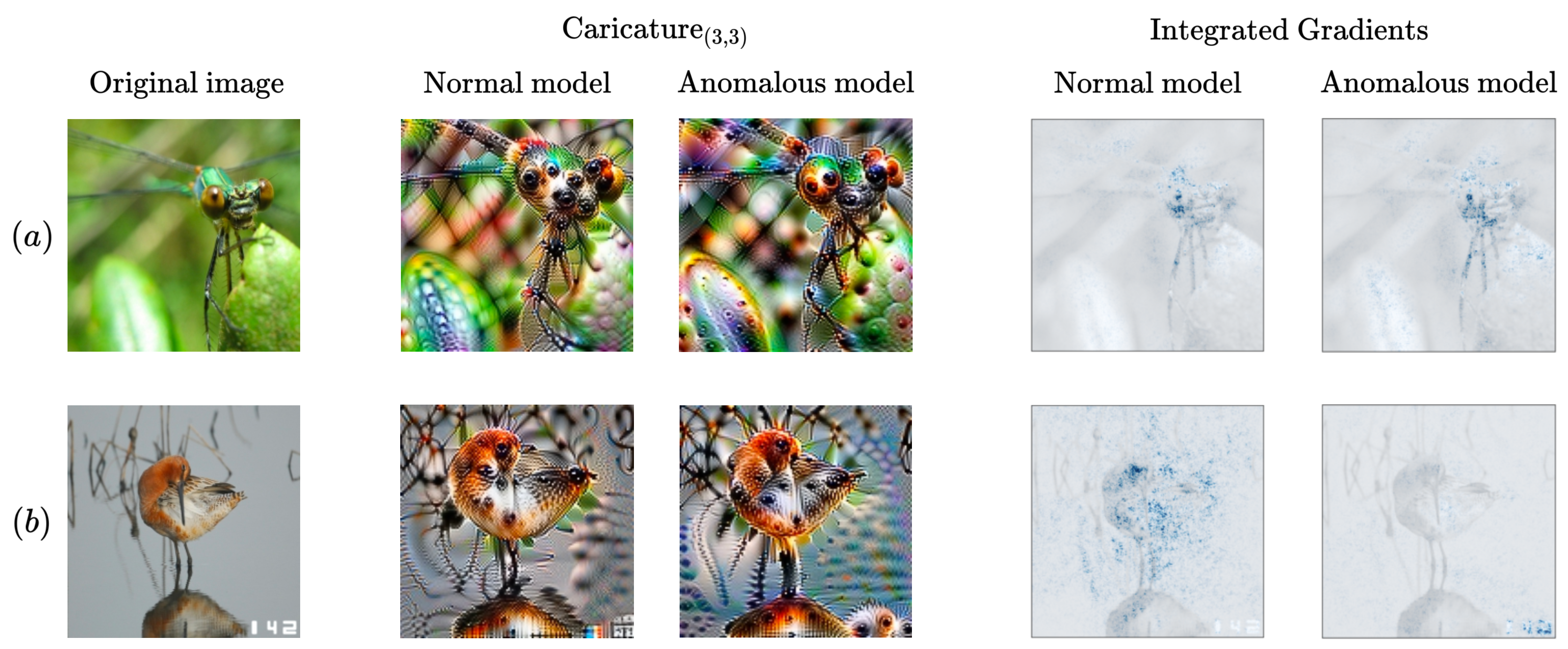
Figure 4: An example where one method can localize abnormal inputs but another method cannot. We show explanations by Caricatures (layer (3,3)) and Integrated Gradients of a reference model and Spurious Feature model ($\delta=0.3$) on a normal image $(a)$ and an abnormal image $(b)$. For IntGrad, the anomalous and normal models’ explanations appear very different for the abnormal image, but not for the normal image. In contrast, for Caricatures the explanations don’t seem more different for the abnormal image: IntGrad can localize the abnormal image, but Caricatures can’t.

Results. We display results in Table 2. We find that no method can localize all of the anomalies, and that the visualizations often have close to random performance. Indeed, only $31\%$ of the AUROCs in Table 2 are greater than 0.7, which we use as a threshold for acceptable classification following (Hosmer Jr. et al., 2013), and $54\%$ are between 0.4 and 0.6. This is especially clear for Missing Class anomalies, where only 2 AUROCs out of 33 exceed 0.7, and all methods generally fail to detect whether an input is from the removed class.

We also find that the feature attribution methods are better than the caricatures at localizing the anomalies. In particular, all of the feature attributions succeed at localization for the Backdoor and Blurred Faces anomalies – achieving AUROCs of at least 0.95 for all the backdoors – whereas most of the caricatures fail. This could be because feature attributions are designed to highlight specific regions inside images, which would include backdoor triggers and faces. However, this explanation should also apply to the Spurious Feature anomalies, on which feature attribution methods do not perform as well. We were also surprised by the AUROC of 0.28 for Caricature_(2,2,1) and the Blurred Faces anomaly, since we don’t see any reason for worse-than-random performance.

Finally, there are some anomalies for which only a couple of methods can distinguish abnormal images. For example, Grad-CAM and Guided Grad-CAM succeed at localization for the model trained without data from the Welsh springer spaniel class, with AUROCs of 0.81 and 0.74, whereas all other methods fail. Similarly for the Spurious Features anomalies (see Figure 4 for qualitative observations), the AUROCs of Guided Backpropagation and Integrated Gradients are greater than 0.75 for $\delta\in\{0.1,0.3,0.5\}$, while the other methods have close to random performance. Surprisingly, the AUROCs tend to be worse for $\delta=1.0$, for example 0.42 for Integrated Gradients, and generally do not increase with $\delta$.

Overall, we find mixed results: although feature attribution methods are able to localize some anomalies (Backdoors and Blurred Faces), no method can localize all of the anomalies, and the feature attribution methods have near-random performance for the majority of anomalies. We show similar results for the other LPIPS metrics in the Appendix (Section A.1.2).

6 Discussion

We have presented a general framework to evaluate model visualizations, grounded in their ability to detect and localize model failures. Given a visualization method $E$ and a metric between visualizations, our scheme provides fine-grained information on $E$’s sensitivity to different anomalies. Applying this framework to feature attribution and feature visualization methods allowed us to discover important shortcomings of these methods.

Are our tests easy or hard? We designed the detection and localization tests to be easy to pass. This means we cannot draw strong conclusions when methods pass them, but that when methods fail at them, this is strong evidence that they are not sensitive enough to the model anomalies.

First, detection should be easy because our reference set of normal models is very narrow. Indeed, the normal models differ only by the random seed used in training, while in reality models vary in architecture, training hyperparameters, etc. According to D’Amour et al. (2020), varying random seed only leads to a 0.001 standard deviation in ImageNet validation accuracy, and an at most 0.024 standard deviations on ImageNet-C stress tests. Moreover, some of our subtle anomalies are not as stealthy as their real-world counterparts: for example, half of our backdoors poison a very large fraction of the training data ($30\%$ to $50\%$), so we should expect them to be fairly easy to detect. Similarly, our localization task is much simpler than localization in real-world settings, where one must proactively anticipate the inputs on which models fail rather than simply recognize them.

Understanding how anomalies change networks. Our results can also help better understand how different anomalies affect the models. For example, Caricatures cannot detect dropping a class from the training dataset: this suggests that this anomaly has only a minor effect on the network’s learned features, likely because most features are shared across different classes. In contrast, Caricatures can detect adversarial training, which corroborates prior work showing that adversarially trained networks learn different, more robust features (Ilyas et al., 2019; Engstrom et al., 2019b).

Future work. One direction for future work is applying this framework to more models: adding new anomalies to detect such as the rewritten models in Santurkar et al. (2021), working with other architectures, and considering different modalities such as natural language or code generation.

Currently, our framework relies heavily on a reference set of “normal models”. This is useful to ground the notion of an anomalous model, and also helps quantify transparency methods’ performance at detection and localization. However, we do not always have such a set of networks at hand. For example, suppose we want to evaluate whether a method can detect the failure modes of a large new model. While this new model may often be “anomalous” compared to reference sets of older models, that is not very relevant to us: we are interested in specific, problematic anomalies. It would therefore be valuable to design frameworks that do not require access to “normal” models, perhaps by replacing the notion of “anomaly” with that of “deviation from a specification”.

Finally, one could extend our framework to evaluate different kinds of visualization methods. For instance, some transparency methods are intrinsic to a model or one of its neurons (Olah et al., 2017), thus obviating the need for input examples. Developing tools to evaluate these input-independent methods could help transparency researchers draw more robust conclusions that are not contingent on a specific choice of samples.

Our results add to the growing body of work on assessing and grounding model transparency methods. We hope this will spur further method development, and aid researchers in their goal of better understanding neural network models.

7 Acknowledgments and Disclosure of Funding

Thanks to Lisa Dunlap, Yaodong Yu, Erik Jones, Suzie Petryk, Xinyan Hu, and Cassidy Laidlaw for comments and feedback. Thanks to Chris Olah, Julius Adebayo, and our anonymous reviewers for helpful discussion. JSD is supported by the NSF Division of Mathematical Sciences Grant No. 2031899.

Appendix A Appendix

A.1 Results with other LPIPS distances

A.1.1 Detection

Table 3: Fraction of anomalous models detected by each method when using AlexNet for the LPIPS distance, with layer-wise Caricature results. The results are similar to those with different LPIPS distances: all methods succeed at the detection task for most stark anomalies, but fail for most of the subtle anomalies.

	Stark Anomalies				Subtle Anomalies
Anomaly Type	Smoothing	Shape Bias	Adv. ($\ell^{\infty}$)	Adv. ($\ell^{2}$)	Backdoor	Spurious	Blur	Missing
GBP	1	1	1	0.75	0.67	0.5	0	0
IntGrad	1	1	1	1	0.17	1	0	0
Grad-CAM	1	1	1	0.75	0.5	0.25	0	0
Guided Grad-CAM	1	1	1	0.75	0.5	0.25	0	0
Car(2,2,1)	1	1	1	0.75	0.5	0.25	0	0
Car(3,0,3)	1	1	1	0.75	0.67	0.25	0	0
Car(3,2,2)	1	1	1	1	0.83	0.5	0	0
Car(3,3)	1	1	1	0.75	0.5	0.25	0	0
Car(3,4,3)	1	1	1	0.75	0	0.25	0	0
Car(4,0,3)	1	1	1	0.75	0.83	0.25	0	0
Car(4,2,3)	1	1	1	0.75	0	0.25	0	0
Car${}_{\text{(all)}}$	1	1	1	1	1	0.25	0	0

Table 4: Fraction of anomalous models detected by each method when using VGG for the LPIPS distance, with layer-wise Caricature results. The results are similar to those with different LPIPS distances: all methods succeed at the detection task for most stark anomalies, but fail for most of the subtle anomalies.

	Stark Anomalies				Subtle Anomalies
Anomaly Type	Smoothing	Shape Bias	Adv. ($\ell^{\infty}$)	Adv. ($\ell^{2}$)	Backdoor	Spurious	Blur	Missing
GBP	1	1	1	0.75	0.17	0.5	0	0.33
IntGrad	1	1	1	1	0.33	1	0	0
Grad-CAM	1	1	1	0.75	0.5	0.25	0	0
Guided Grad-CAM	1	1	1	0.75	0.17	0.25	0	0.33
Car(2,2,1)	1	0	1	0.5	0.33	0	0	0
Car(3,0,3)	1	1	1	1	0.83	0.25	0	0
Car(3,2,2)	1	1	1	1	1	0.25	0	0
Car(3,3)	1	1	1	0.75	0.83	0.25	0	0
Car(3,4,3)	1	1	1	0.5	0	0.25	0	0
Car(4,0,3)	1	1	1	0.75	0.83	0.5	0	0
Car(4,2,3)	1	1	1	0.75	0.17	0.25	0	0
Car${}_{\text{(all)}}$	1	1	1	0.75	0.83	0.25	0	0

Table 5: Fraction of anomalous models detected by each method when using SqueezeNet for the LPIPS distance, with layer-wise Caricature results. The results are similar to those with different LPIPS distances: all methods succeed at the detection task for most stark anomalies, but fail for most of the subtle anomalies.

	Stark Anomalies				Subtle Anomalies
Anomaly Type	Smoothing	Shape Bias	Adv. ($\ell^{\infty}$)	Adv. ($\ell^{2}$)	Backdoor	Spurious	Blur	Missing
GBP	1	1	1	0.75	0.83	0.75	0	0.33
IntGrad	1	1	1	1	0.17	1	0	0
Grad-CAM	1	1	1	0.75	0.5	0.25	0	0
Guided Grad-CAM	1	1	1	0.75	0.17	0.25	0	0
Car(2,2,1)	1	0	1	0.5	0.67	0.25	0	0
Car(3,0,3)	1	1	1	1	0.83	0.25	0	0
Car(3,2,2)	1	1	1	1	0.83	0.25	0	0
Car(3,3)	1	1	1	0.75	0.67	0.5	0	0
Car(3,4,3)	1	1	1	0.5	0	0.25	0	0
Car(4,0,3)	1	1	1	0.5	0.83	0.5	0	0
Car(4,2,3)	1	1	1	1	0.17	0.5	1	0
Car${}_{\text{(all)}}$	1	1	1	0.75	1	0.25	0	0

A.1.2 Localization

Table 6: Localization AUROC (%) using the VGG-LPIPS distance for every anomaly and explanation method, with AUROCs higher than 70% bolded. Although feature attributions successfully localize the backdoors, no method can localize all of the anomalies, and visualizations often have close to random performance.

Category	Backdoor						Missing class			Spurious				Blur
Anomaly	0	1	2	3	4	5	218	400	414	0.1	0.3	0.5	1.0
GBP	100	100	99	100	99	100	66	44	55	66	77	66	66	88
IntGrad	97	92	91	96	96	83	55	55	44	77	66	77	33	77
Grad-CAM	98	98	94	97	99	96	88	55	55	55	55	55	55	77
Guided Grad-CAM	99	100	92	100	99	100	77	33	55	55	66	55	44	77
Car(2,2,1)	53	47	51	48	50	56	33	66	77	55	44	44	55	33
Car(3,0,3)	53	48	55	47	53	54	44	44	44	44	55	44	55	55
Car(3,2,2)	55	62	56	51	43	57	44	55	33	44	55	44	55	44
Car(3,3)	52	74	81	61	80	63	44	44	66	66	44	44	55	88
Car(3,4,3)	60	68	68	61	72	62	66	55	33	44	44	44	44	55
Car(4,0,3)	58	74	79	63	88	66	66	33	44	55	55	44	55	66
Car(4,2,3)	98	98	97	96	88	87	44	55	66	55	55	44	55	66

Table 7: Localization AUROC (%) using the SqueezeNet-LPIPS distance for every anomaly and explanation method, with AUROCs higher than 70% bolded. Although feature attributions successfully localize the backdoors, no method can localize all of the anomalies, and visualizations often have close to random performance.

Category	Backdoor						Missing class			Spurious				Blur
Anomaly	0	1	2	3	4	5	218	400	414	0.1	0.3	0.5	1.0
GBP	100	100	100	100	100	100	67	42	58	74	79	75	64	84
IntGrad	100	98	99	99	99	96	61	63	46	85	81	87	35	90
Grad-CAM	98	98	95	97	99	97	80	58	58	52	53	51	53	76
Guided Grad-CAM	99	100	97	100	100	100	70	39	56	56	71	63	58	79
Car(2,2,1)	50	45	55	47	52	50	49	41	66	45	44	55	59	24
Car(3,0,3)	60	50	60	43	50	49	45	49	55	56	55	44	53	66
Car(3,2,2)	57	52	58	55	47	46	58	70	34	54	60	46	49	50
Car(3,3)	49	58	71	63	73	62	45	51	65	55	59	38	55	86
Car(3,4,3)	67	60	58	64	83	63	67	63	58	44	51	43	35	57
Car(4,0,3)	61	62	75	56	77	70	53	26	49	52	49	45	50	59
Car(4,2,3)	91	63	92	91	84	81	55	51	53	56	53	51	41	55

A.2 More details on the models

Normal models: We trained the normal models with a batch size of 300. Other than that, we used the same hyperparameters as PyTorch’s (Paszke et al., 2019) pretrained ResNet-50: we did 90 epochs of SGD with momentum $0.9$ and a weight decay of $0.0001$. Our initial learning rate was 0.1, and we multiplied it by 0.1 every 30 epochs. We used the exact same parameters when training the backdoored, spurious features, missing class, and blurred faces anomalous models.

Adversarial Training: The $\ell^{2}$ adversarially trained models were trained with the same hyperparameters, except for the batch size which was equal to 512 (Salman et al., 2020). The $\ell^{\infty}$ adversarially trained models were also trained with the same hyperparameters as the PyTorch pretrained ResNet-50 (Engstrom et al., 2019a).

Shape Bias: We used the checkpoint from Geirhos et al. (2019). This was not trained using the exact same hyperparameters as the PyTorch pretrained ResNet-50: training on Stylized ImageNet was done for 60 rather than 90 epochs, they used a batch size of 256 and multiplied the learning rate by 0.1 after 20 and 40 epochs. The other hyperparameters were the same: SGD with momentum $0.9$, weight decay $0.0001$, initial learning rate of $0.1$.

Backdoored models: To train the backdoored models, we select a fraction $\nu$ of the images in each batch, add the trigger to it, and replace its label by a preset target label. We train 6 backdoored models, indexed from 0 to 5. Figure 5 below shows for each backdoored model, an example of an image with the trigger, as well as the value of $\nu$.

(a) Backdoor 0: $\nu=0.5$

(b) Backdoor 1: $\nu=0.1$

(c) Backdoor 2: $\nu=0.05$

(d) Backdoor 3: $\nu=0.3$

(e) Backdoor 4: $\nu=0.01$

(f) Backdoor 5: $\nu=0.5$

Figure 5: Images with the different backdoored models’ triggers.

Spurious Features: To train the models with spurious features, we select a fraction $\delta$ of the images in each batch, and overlay the corresponding class index on the bottom right of the image. Figure 6 shows an example of an image with the spurious feature.

Figure 6: Image with the spurious cue.

References

- Adebayo et al. (2018) Julius Adebayo, Justin Gilmer, Michael Muelly, Ian Goodfellow, Moritz Hardt, and Been Kim. Sanity checks for saliency maps. In Proceedings of the 32nd International Conference on Neural Information Processing Systems, NIPS’18, 2018.
- Adebayo et al. (2020) Julius Adebayo, Michael Muelly, Ilaria Liccardi, and Been Kim. Debugging tests for model explanations, 2020.
- Adebayo et al. (2022) Julius Adebayo, Michael Muelly, Harold Abelson, and Been Kim. Post hoc explanations may be ineffective for detecting unknown spurious correlation. In International Conference on Learning Representations, 2022. URL https://openreview.net/forum?id=xNOVfCCvDpM.
- Bagdasaryan & Shmatikov (2021) Eugene Bagdasaryan and Vitaly Shmatikov. Blind backdoors in deep learning models. In 30th USENIX Security Symposium (USENIX Security 21). USENIX Association, August 2021.
- Bastings et al. (2021) Jasmijn Bastings, Sebastian Ebert, Polina Zablotskaia, Anders Sandholm, and Katja Filippova. "will you find these shortcuts?" a protocol for evaluating the faithfulness of input salience methods for text classification, 2021.
- Bhatt et al. (2020) Umang Bhatt, Alice Xiang, Shubham Sharma, Adrian Weller, Ankur Taly, Yunhan Jia, Joydeep Ghosh, Ruchir Puri, José M. F. Moura, and Peter Eckersley. Explainable machine learning in deployment, 2020.
- Cammarata et al. (2021) Nick Cammarata, Gabriel Goh, Shan Carter, Chelsea Voss, Ludwig Schubert, and Chris Olah. Curve circuits. Distill, 2021. URL https://distill.pub/2020/circuits/curve-circuits.
- Casper et al. (2023) Stephen Casper, Yuxiao Li, Jiawei Li, Tong Bu, Kevin Zhang, and Dylan Hadfield-Menell. Benchmarking interpretability tools for deep neural networks, 2023.
- Cohen et al. (2019) Jeremy M Cohen, Elan Rosenfeld, and J. Zico Kolter. Certified adversarial robustness via randomized smoothing, 2019.
- D’Amour et al. (2020) Alexander D’Amour, Katherine Heller, Dan Moldovan, Ben Adlam, Babak Alipanahi, Alex Beutel, Christina Chen, Jonathan Deaton, Jacob Eisenstein, Matthew D. Hoffman, Farhad Hormozdiari, Neil Houlsby, Shaobo Hou, Ghassen Jerfel, Alan Karthikesalingam, Mario Lucic, Yian Ma, Cory McLean, Diana Mincu, Akinori Mitani, Andrea Montanari, Zachary Nado, Vivek Natarajan, Christopher Nielson, Thomas F. Osborne, Rajiv Raman, Kim Ramasamy, Rory Sayres, Jessica Schrouff, Martin Seneviratne, Shannon Sequeira, Harini Suresh, Victor Veitch, Max Vladymyrov, Xuezhi Wang, Kellie Webster, Steve Yadlowsky, Taedong Yun, Xiaohua Zhai, and D. Sculley. Underspecification presents challenges for credibility in modern machine learning, 2020.
- Ding et al. (2021) Frances Ding, Jean-Stanislas Denain, and Jacob Steinhardt. Grounding representation similarity with statistical testing, 2021.
- Doshi-Velez & Kim (2017) Finale Doshi-Velez and Been Kim. Towards a rigorous science of interpretable machine learning, 2017.
- Engstrom et al. (2019a) Logan Engstrom, Andrew Ilyas, Hadi Salman, Shibani Santurkar, and Dimitris Tsipras. Robustness (Python Library), 2019a. URL https://github.com/MadryLab/robustness.
- Engstrom et al. (2019b) Logan Engstrom, Andrew Ilyas, Shibani Santurkar, Dimitris Tsipras, Brandon Tran, and Aleksander Madry. Adversarial robustness as a prior for learned representations, 2019b.
- Geirhos et al. (2019) Robert Geirhos, Patricia Rubisch, Claudio Michaelis, Matthias Bethge, Felix A. Wichmann, and Wieland Brendel. ImageNet-trained CNNs are biased towards texture; increasing shape bias improves accuracy and robustness, 2019.
- Gildenblat & contributors (2021) Jacob Gildenblat and contributors. Pytorch library for CAM methods. https://github.com/jacobgil/pytorch-grad-cam, 2021.
- Hernandez et al. (2022) Evan Hernandez, Sarah Schwettmann, David Bau, Teona Bagashvili, Antonio Torralba, and Jacob Andreas. Natural language descriptions of deep visual features, 2022.
- Hosmer Jr. et al. (2013) David W Hosmer Jr., Stanley Lemeshow, and Rodney X Sturdivant. Applied logistic regression, volume 398. John Wiley & Sons, 2013.
- Ilyas et al. (2019) Andrew Ilyas, Shibani Santurkar, Dimitris Tsipras, Logan Engstrom, Brandon Tran, and Aleksander Madry. Adversarial examples are not bugs, they are features, 2019.
- Kiat (2021) Lim Swee Kiat. Lucent, Lucid library adapted for pytorch, 2021.
- Koh et al. (2020) Pang Wei Koh, Thao Nguyen, Yew Siang Tang, Stephen Mussmann, Emma Pierson, Been Kim, and Percy Liang. Concept bottleneck models, 2020.
- Kokhlikyan et al. (2020) Narine Kokhlikyan, Vivek Miglani, Miguel Martin, Edward Wang, Bilal Alsallakh, Jonathan Reynolds, Alexander Melnikov, Natalia Kliushkina, Carlos Araya, Siqi Yan, and Orion Reblitz-Richardson. Captum: A unified and generic model interpretability library for PyTorch, 2020.
- Li et al. (2021) Yiming Li, Baoyuan Wu, Yong Jiang, Zhifeng Li, and Shu-Tao Xia. Backdoor learning: A survey, 2021.
- Lin et al. (2020) Yi-Shan Lin, Wen-Chuan Lee, and Z. Berkay Celik. What do you see? evaluation of explainable artificial intelligence (XAI) interpretability through neural backdoors, 2020.
- Madry et al. (2019) Aleksander Madry, Aleksandar Makelov, Ludwig Schmidt, Dimitris Tsipras, and Adrian Vladu. Towards deep learning models resistant to adversarial attacks, 2019.
- Molnar (2022) Christoph Molnar. Interpretable Machine Learning. 2 edition, 2022. URL https://christophm.github.io/interpretable-ml-book.
- Olah (2018) Chris Olah. Research: Caricatures, 2018. URL https://github.com/tensorflow/lucid/issues/121.
- Olah et al. (2017) Chris Olah, Alexander Mordvintsev, and Ludwig Schubert. Feature visualization. Distill, 2017. URL https://distill.pub/2017/feature-visualization.
- Paszke et al. (2019) Adam Paszke, Sam Gross, Francisco Massa, Adam Lerer, James Bradbury, Gregory Chanan, Trevor Killeen, Zeming Lin, Natalia Gimelshein, Luca Antiga, Alban Desmaison, Andreas Kopf, Edward Yang, Zachary DeVito, Martin Raison, Alykhan Tejani, Sasank Chilamkurthy, Benoit Steiner, Lu Fang, Junjie Bai, and Soumith Chintala. PyTorch: An imperative style, high-performance deep learning library, 2019. URL http://papers.neurips.cc/paper/9015-pytorch-an-imperative-style-high-performance-deep-learning-library.pdf.
- Salman et al. (2020) Hadi Salman, Andrew Ilyas, Logan Engstrom, Ashish Kapoor, and Aleksander Madry. Do adversarially robust ImageNet models transfer better?, 2020.
- Santurkar et al. (2021) Shibani Santurkar, Dimitris Tsipras, Mahalaxmi Elango, David Bau, Antonio Torralba, and Aleksander Madry. Editing a classifier by rewriting its prediction rules, 2021.
- Selvaraju et al. (2019) Ramprasaath R. Selvaraju, Michael Cogswell, Abhishek Das, Ramakrishna Vedantam, Devi Parikh, and Dhruv Batra. Grad-CAM: Visual explanations from deep networks via gradient-based localization. International Journal of Computer Vision, 128(2):336–359, Oct 2019. URL https://doi.org/10.1007%2Fs11263-019-01228-7.
- Singla & Feizi (2021) Sahil Singla and Soheil Feizi. Salient ImageNet: How to discover spurious features in deep learning?, 2021.
- Springenberg et al. (2015) Jost Tobias Springenberg, Alexey Dosovitskiy, Thomas Brox, and Martin Riedmiller. Striving for simplicity: The all convolutional net, 2015.
- Sundararajan et al. (2017) Mukund Sundararajan, Ankur Taly, and Qiqi Yan. Axiomatic attribution for deep networks, 2017.
- Taori et al. (2020) Rohan Taori, Achal Dave, Vaishaal Shankar, Nicholas Carlini, Benjamin Recht, and Ludwig Schmidt. Measuring robustness to natural distribution shifts in image classification. In Advances in Neural Information Processing Systems (NeurIPS), 2020. URL https://arxiv.org/abs/2007.00644.
- Wong et al. (2021) Eric Wong, Shibani Santurkar, and Aleksander Mądry. Leveraging sparse linear layers for debuggable deep networks, 2021.
- Yang et al. (2021) Kaiyu Yang, Jacqueline Yau, Li Fei-Fei, Jia Deng, and Olga Russakovsky. A study of face obfuscation in ImageNet, 2021.
- Zhang et al. (2018) Richard Zhang, Phillip Isola, Alexei A. Efros, Eli Shechtman, and Oliver Wang. The unreasonable effectiveness of deep features as a perceptual metric, 2018.
- Zhou et al. (2021) Yilun Zhou, Serena Booth, Marco Tulio Ribeiro, and Julie Shah. Do feature attribution methods correctly attribute features?, 2021.