New heuristic to choose a cylindrical algebraic decomposition variable ordering motivated by complexity analysis

Abstract

It is well known that the variable ordering can be critical to the efficiency or even tractability of the cylindrical algebraic decomposition (CAD) algorithm. We propose new heuristics inspired by complexity analysis of CAD to choose the variable ordering. These heuristics are evaluated against existing heuristics with experiments on the SMT-LIB benchmarks using both existing performance metrics and a new metric we propose for the problem at hand. The best of these new heuristics chooses orderings that lead to timings on average 17% slower than the virtual-best: an improvement compared to the prior state-of-the-art which achieved timings 25% slower.

1 Introduction

1.1 Cylindrical algebraic decomposition

A Cylindrical Algebraic Decomposition (CAD) of $\mathbb{R}^{n}$ is a decomposition of $\mathbb{R}^{n}$ into semi-algebraic cells that are cylindrically arranged. A cell being semi-algebraic means that it can be described by polynomial constraints. CADs are defined relative to a variable ordering, for example, $x_{n}\succ x_{n-1}\succ\dots\succ{x_{1}}$. Then the cylindrical property means that the projections of any two cells in $\mathbb{R}^{n}$ onto a subspace $\mathbb{R}^{i},i<n$ with respect to this variable ordering, are either equal or disjoint. I.e. the cells in $\mathbb{R}^{n}$ are arranged into cylinders above cells in $\mathbb{R}^{n-1}$, which are themselves arranged into cylinders above $\mathbb{R}^{n-2}$ and so on.

It can be very useful to find such decompositions satisfying a property such as sign-invariance for an input set of polynomials (i.e. each polynomial has constant sign in each cell). The principle is that given an infinite space, a sign-invariant decomposition gives a finite set of regions on each of which our system of study has invariant behaviour, and thus can be analyzed by testing a single sample point. When such a decomposition is also cylindrical and semi-algebraic we can use it to perform tasks like quantifier elimination.

Collins in 1975 [Collins1975] was the first to propose a feasible algorithm to build such sign-invariant decompositions for a given set of polynomials. This algorithm has two phases, projection and lifting, each of them consisting of $n$ steps, where $n$ is the number of variables in the given set of polynomials $S_{n}$.

In the first step of the projection phase the given set of polynomials, $S_{n}$ is passed to a CAD projection operator to obtain a set of polynomials $S_{n-1}$ in $n-1$ variables (without the biggest variable $x_{n}$). This process is iterated until a set of polynomials $S_{1}$ only in the variable ${x_{1}}$ is left: at this point the projection phase ends.

In the first step of the lifting phase a CAD of $\mathbb{R}^{1}$ is created by computing the $t$ ordered roots of $S_{1}$, denoted $r_{1},\dots,r_{t}$, and building the CAD of $\mathbb{R}^{1}$ out of the cells $(-\infty,r_{1}),[r_{1}],(r_{1},r_{2}),\dots,(r_{n-1},r_{n}),[r_{n}],(r_{n},\infty)$. Note that a sample point can be taken from each of those cells.

For each of those cells, the sample point is substituted into the set of polynomials $S_{2}$ to obtain a set of polynomials in one variable. Then using this set a stack of cells is built on top of each cell by following the instructions in the previous paragraph. These stacks are combined later into a CAD of $\mathbb{R}^{2}$ and by iterating this process a CAD of $\mathbb{R}^{n}$ is eventually built, concluding the lifting phase and the algorithm.

The proof of correctness of CAD (allowing the conclusion of sign-invariance) relies on proving that the decompositions built over the sample point are representative of the behaviour over the entire cell: to conclude this the projection operator must produce polynomials whose zeros indicate where the behaviour would change. One representation of a CAD is as a tree of cells of increasing dimension; whose leaves are the cells in $\mathbb{R}^{n}$, nodes the cells in lower dimension, and branches representing the cylinders over projections.

Since the introduction of CAD by Collins, many improvements have been made to the algorithm. We do not detail them all here but refer the reader to the overview of the first 20 years in [Collins1998] and to e.g. the introduction of [Bradford2016] for some of the more recent advances. We note in particular the recent developments in CAD projection [McCallum2019] and the recent application of CAD technology within SMT and verification technology e.g. [Kremer2020], [Abraham2021] which has inspired new adaptations of the CAD algorithm such as [Brown2015]. The work of this paper is presented for traditional CAD, but we expect it would transfer easily to these recent contexts.

1.2 CAD variable ordering

It is well known that the variable ordering given can have a huge impact on the time and resources needed to build the CAD (see e.g. [Dolzmann2004], [England2019], [Huang2019]). We demonstrate this for a very simple example in Figure 1, where one choice leads to three times the number of cells than the other. In fact, [Brown2007] shows that the choice of variable ordering can even change the theoretical complexity for certain classes of problems.

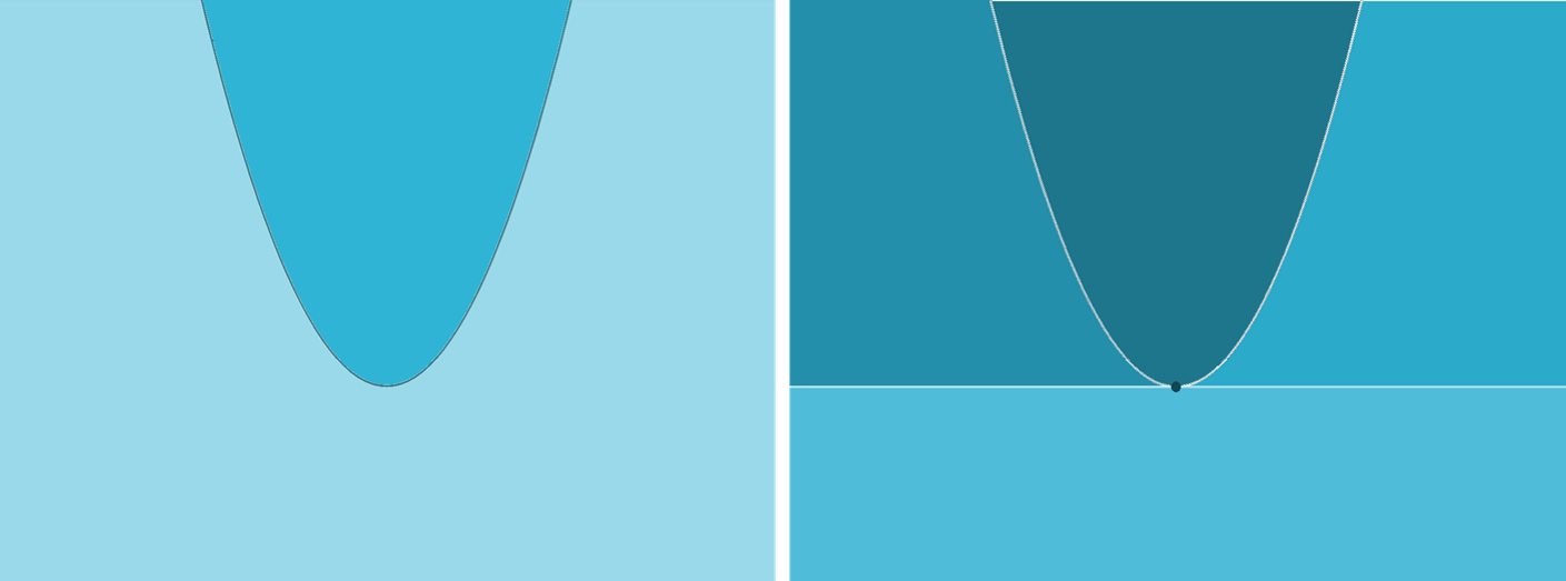
Figure 1: CADs sign-invariant for $x^{2}-y$ in the two possible orderings. The ordering $y\succ x$ generates the CAD on the left with only three cells (the coloured regions and the curve between). The ordering $x\succ y$ generates the CAD on the right with nine cells (the four coloured regions along with four line segments and the turning point of the curve).

Depending on the application the CAD is to be used for, we have a free or constrained choice of variable ordering. For example, to use a CAD for real quantifier elimination it is necessary to project variables in the order they are quantified, but there is freedom to swap the order of variables in quantifier blocks, and also to swap the order of the free (unquantified) variables and parameters. Making use of this freedom is an important optimisation. This paper aims to present a new heuristic to pick the variable ordering for the construction of a CAD.

1.3 Plan of the paper

We continue in Section 2 by describing the previous heuristics developed for the problem. Then in Section 3 the proposed heuristics are presented. We then move onto our experimental evaluation: in Section 4 the methodology is detailed and in Section 5 the results obtained are analyzed. We finish with our conclusions and suggestions for future work in Section LABEL:sec:final.

2 Previous heuristics

Due to how critical the variable ordering can be, a variety of heuristics have already been proposed for making the choice. We will focus on two of these which are widely considered to constitute the current state-of-the-art: the Brown heuristic, presented in [Brown2004], and sotd, presented in [Dolzmann2004]. We describe these in full over the coming subsections.

We acknowledge there are additional human-designed heuristics in the literature, but these are either even more expensive than sotd e.g. [Bradford2013], [Wilson2015], or designed relative to a very specific CAD implementation e.g. [England2014].

We also acknowledge that there exists a family of machine learning methods to take this decisions e.g. [Huang2019], [England2019], [Florescu2019b], [Chen2020], [Brown2020] which have been shown to outperform the human-designed heuristics. We do not compare against these directly but note that the lessons learnt in this paper could inform another generation of these machine learnt heuristics.

2.1 The Brown heuristic

The Brown heuristic was proposed by Brown in the notes to his ISSAC 2004 tutorial [Brown2004, Section 5.2]. It chooses to project the variable with:

1. lowest degree; breaking ties with

2. lowest value of the highest total degree term in which the variable appears; breaking ties with

3. lowest number of terms containing the variable.

Should there remain ties after the third measure then [Brown2004] does not specify what to do: we name the variables $x_{1},x_{2},\dots$ according to the order in which they appear in the description of the problem and our implementation of the Brown heuristic chooses the variable with the lowest subindex first.

The text in [Brown2004] is also unclear on whether these measures are applied only to the input polynomials to produce the complete ordering, or whether they are applied to select an ordering one variable at a time, each time being applied to the polynomials obtained from projection with the last variable. Our implementation does the latter: this requires no additional projection computation above that required to build a single CAD, and matches the projection computation used by our new heuristic allowing for a fair comparison later.

For an example, let us consider the set $S_{3}=\{{x_{3}}^{3}+{x_{2}}^{3}+{x_{2}}-{x_{1}}^{4},{x_{2}}^{3}-{x_{1}}\}$. In $S_{3}$ the variable ${x_{1}}$ has degree $4$, but ${x_{3}}$ and ${x_{2}}$ both have degree $3$ so they tie in the first feature. However, ${x_{3}}$ reaches this maximum in only one term, while ${x_{2}}$ does so in two of them and hence ${x_{3}}$ will be the first CAD projected variable. The CAD projection of $S_{3}$ with respect to ${x_{3}}$ is $S_{2}=\{{x_{2}}^{3}+{x_{2}}-{x_{1}}^{4},{x_{2}}^{3}-{x_{1}}\}$. In $S_{2}$ the variable ${x_{1}}$ has degree $4$ while ${x_{2}}$ has degree $3$, so ${x_{2}}$ is the second variable to be projected. This determines the variable ordering chosen with our implementation of the Brown heuristic: ${x_{3}}\succ{x_{2}}\succ{x_{1}}$.

The motivation of the Brown heuristic is to try to make the next projected set of polynomials as small as possible. The heuristic is “cheap” as the measures it uses require only easy to calculate characteristics of the input polynomials, and no algebraic computations such as projection.

Moreover, the Brown heuristic has been shown to achieve similar accuracy to more complicated heuristics [Huang2019], [Florescu2019a], like the one introduced in the next section. This means that when we include the cost of running the heuristics themselves, the Brown heuristic is actually superior.

Nevertheless, as will be seen later, it is possible to propose better heuristics by looking at the bigger picture rather than focusing on the next projected set.

2.2 The sotd heuristics

The acronym sotd stands for ‘sum of total degrees’. The heuristic sotd consists of computing the whole CAD projection of the input polynomials in every possible variable ordering and choosing the ordering whose projection has the smallest sum of total degrees throughout all the monomials in all the polynomials of the projection [Dolzmann2004].

For example, given the set of polynomials $S_{3}$ defined above and following variable ordering ${x_{3}}\succ{x_{1}}\succ{x_{2}}$, then we find $S_{2}$ as defined above and them projection with respect to ${x_{1}}$ gives $S_{1}=\{{x_{2}},{x_{2}}^{2}+1,{x_{2}}^{11}-{x_{2}}^{2}-1\}$. The sum of all the degrees in the projected sets for this ordering is $43$. It turns out that this is lowest such value possible from any of the six possible orderings. Hence the sotd heuristic would choose this variable ordering.

This heuristic is not very desirable at first glance, because $\mathcal{O}(n!)$ projection steps are needed to make the choice, far more than the $n$ projections used to make a single CAD. This problem was spotted by the authors of [Dolzmann2004] leading them to develop a “greedy” version of the heuristic in the same paper. This was greedy in the sense that instead of selecting the entire ordering at once using information from the whole projection phase for each possible ordering; it computed the ordering one variable at a time by comparing their metric on the output of a single projection step for each possible variable from the remaining ones. This version only requires $\frac{n(n+1)}{2}$ number of projections, still more than the amount of projection normally used to build a CAD. In our experiments, the choices it makes are much poorer than those made by sotd with the full projection information. In fact, some experiments show it even performs worse than the Brown heuristic, despite having more projection information available to make its choice. We see this later in our experiments (Table LABEL:tab:allvsallInf0).

The metric sotd, i.e. summing all the degrees in a set of polynomials, was originally constructed as a measure of the overall size of a polynomial set. In [Dolzmann2004] it was used along with other measures to demonstrate the effect of variable ordering on CAD computation. It was found to have a strong correlation with those other CAD complexity measures, but unlike them, it did not require the computation of the entire CAD. This led to its proposal for using it as a heuristic.

Thus, it seems the sotd measure was not designed primarily for use in a CAD variable ordering heuristics, allowing a gap for the new results of the present paper which presents a measure that is designed this way. This lack of tailoring to CAD can be seen in the way sotd and its greedy version give the same importance to all degrees found in the projected sets of polynomials regardless of the variable carrying that degree, whereas CAD works iteratively one variable at a time (treating the others as part of the coefficients when projection and substituting them for the sample point when lifting). Thus different variables carry different weights of effect on CAD computation.

In the next section, it will be shown how better heuristics can be proposed which take into account the potential growth in complexity of the polynomials we observe in CAD projection.

3 Our new proposed heuristics

It has been shown in [Dolzmann2004] that the number of cells of a CAD is strongly correlated with the time taken to build that CAD. Hence the most recent CAD complexity analyses in e.g. [England2015], [Bradford2016], [England2020], [Li2021] have studied a bound on the maximum number of cells that can be generated.

The idea of the proposed heuristic is to make a corresponding estimate on this maximum number of cells of the final CAD for each of the possible orderings and pick the ordering that minimizes this value.

We explain how this number can be computed or estimated if the whole CAD projection is known for each ordering. However, as CAD projection of polynomials can be an expensive operation, a greedy version of this heuristic that does not require any CAD projections to make the choice is also proposed.

3.1 Heuristic motivated by a complexity analysis: mods

Define the degree sum of a variable $x$ in a set of polynomials $S=\{p_{1},\dots,p_{n}\}$ as

$$D_{x}(S)=\sum_{i=1}^{n}d_{x}(p_{i}),$$ (1)

where $d_{x}(p)$ is the degree of $x$ in the polynomial $p$. Thus the maximum number of unique real roots that the polynomials in $S$ can have with respect to $x$, is $D_{x}(S)$.

To compute a CAD with the variable ordering $x_{n}\succ\dots\succ x_{1}$ for the set of polynomials $S_{n}$, the set $S_{n}$ must be projected with respect to $x_{n}$ to obtain the set $S_{n-1}$; and in the same fashion the sets $S_{n-2},S_{n-3},\dots,S_{1}$ are computed.

Thus when following the creation of a CAD as described in Section 1, in the first lifting step at most $2D_{{x_{1}}}(S_{1})+1$ cells can be created because ${x_{1}}$ will have at most $D_{{x_{1}}}(S_{1})$ roots in $S_{1}$. Subsequently at most $(2D_{{x_{1}}}(S_{1})+1)\cdot(2D_{x_{2}}(S_{2})+1)$ cells will be built in the second lifting step (a similar limit applied for each stack above a cell from $\mathbb{R}^{1}$).

Hence, at the end of the lifting phase, when the CAD is completed, an upper bound on the number of cells is

$$\prod_{i=1}^{n}\big{(}2D_{x_{i}}(S_{i})+1\big{)}.$$ (2)

As discussed earlier, the number of cells in a CAD is strongly correlated with the time needed to build such CAD. Therefore, choosing the ordering that minimizes the maximum number of cells in the final CAD sounds like a good idea if we want to choose a fast ordering. Hence, we want to choose the ordering that minimizes (2).

We note that the dominant term of (2) is

$$\prod_{i=1}^{n}D_{x_{i}}(S_{i}),$$ (3)

which we refer to as the multiplication of degree sum (mods). By minimising (2) we are likely minimising this and so we refer to the heuristic that picks an ordering to minimise (2) as mods. As with our implementation of the Brown heuristic, we apply this to choose one variable at a time, projecting with respect to that variable after the choice and then applying the measure to the projection polynomials to make the next choice. In case where there is a tie on the measure then we pick the variable with the lowest subindex.

Consider our example set of polynomials $S_{3}=\{{x_{3}}^{3}+{x_{2}}^{3}+{x_{2}}-{x_{1}}^{4},{x_{2}}^{3}-{x_{1}}\}$. The degree sum of ${x_{1}}$ in $S_{3}$ is

$$D_{x_{e}}(S_{3})=d_{x_{e}}({x_{3}}^{3}+{x_{2}}^{3}+{x_{2}}-{x_{1}}^{4})+d_{x_{e}}({x_{2}}^{3}-{x_{1}})=3+0=3.$$

Suppose we built a CAD using the variable ordering ${x_{3}}\succ{x_{1}}\succ{x_{2}}$. Then as before we obtain $S_{2}=\{-{x_{2}}^{3}+{x_{1}},{x_{1}}^{4}-{x_{2}}^{3}-{x_{2}}\}$ for which $D_{{x_{1}}}(S_{2})=5$, and $S_{1}=\{{x_{2}},{x_{2}}^{2}+1,{x_{2}}^{11}-{x_{2}}^{2}-1\}$ for which $D_{x_{2}}(S_{1})=14$. Therefore, for this example CAD the product (2) evaluates to 2233. It turns out that is the lowest value of (2) for all the possible orderings. Hence mods would have chosen this ordering.

3.2 Creating a greedy version of mods

As with sotd, the heuristic mods is relatively expensive, requiring the use of CAD projection operations in all different variable orderings. To reduce its cost we present a greedy version of this heuristic, that will simply choose to project the variable with the lowest degree sum (see ((1))) in the set of polynomials

This heuristic will be referred to as gmods. Note that unlike greedy-sotd, gmods does not use any projection information beyond that required to build a single CAD. The metric it is based on uses only easily extracted information from the polynomials. It is thus similar in cost to our implementation of the Brown heuristic.

For example, given the set of polynomials $S_{3}$ above we have $D_{x_{1}}(S_{3})=5$, $D_{x_{2}}(S_{3})=6$ and $D_{x_{3}}(S_{3})=3$. Thus gmods will select ${x_{3}}$ as the first variable for CAD projection. The CAD projection of $S_{3}$ with respect to ${x_{3}}$ gives $S_{2}$ as above. In $S_{2}$ the variable ${x_{1}}$ has degree sum $5$ while ${x_{2}}$ has degree sum $6$, so ${x_{1}}$ is the second variable to be projected, determining completely the variable ordering that gmods chooses: ${x_{3}}\succ{x_{1}}\succ{x_{2}}$.

3.3 Heuristic motivated by expected number of cells

Our mods heuristic is motivated to reduce the maximum number of cells that could be computed according to a complexity analysis. It is natural to ask whether we could be more accurate and seek take decisions according to an expected value of the number of cells rather than the maximum?

To calculate the maximum number of cells that can be generated, the degree of the polynomials has been used because it is the maximum number of real roots that a polynomial can have, so we may consider the expected number of roots of a polynomial. According to [Fairley1976], the expected number of real roots for polynomials of small degree is proportional to the logarithm of its degree, at least for their definition of random polynomials. However, for a linear polynomial, this relation would predict zero roots when it should be one, and so to address this we suggest a heuristic following this approach should add one before taking the logarithm.

Thus we hypothesise an expected number of cells in the final CAD as below (following the approach of Section 3.1):

$$\prod_{i=1}^{n}(2\log(D_{x_{i}}(S_{i})+1)+1).$$ (4)

As before, we define a heuristic to pick the ordering that minimizes (4). Given the similarity to mods and the use of the logarithm we refer to this as logmods.

For example, consider the set of polynomials $S_{3}$ as before and the variable ordering ${x_{3}}\succ{x_{1}}\succ{x_{2}}$ to produce $S_{2}$ and $S_{1}$ as before. We find $D_{x_{3}}(S_{3})=3$, $D_{x_{1}}(S_{2})=5$, and $D_{x_{2}}(S_{1})=14$. Therefore, (4) evaluates to $15.43$, and it turns out that is the lowest value for all possible orderings, hence, logmods would choose this variable ordering.

4 Experiments and benchmarking

4.1 Benchmarking

The three-variable problems in the QF_NRA category of the SMT-LIB [Barrett2016] are used to build a dataset for comparing the different heuristics.

For each of those problems and all possible orderings, we timed (see Section 4.1.2) how long it takes to build a sign-invariant CAD for the polynomials involved, discarding the problems in which the creation of the CAD timed out for all orderings. After building all the possible CADs, a dataset of “unique” problems is created (see Section 4.1.3).

Of the 5942 original problems, in 343 of them, all the orderings timed out. And out of the remaining 5599 problems, only 1019 unique problems were found. These 1019 problems will be used as benchmarks to compare the heuristics presented in Sections 2 and 3.

4.1.1 CAD Implementation

For our experiments we used the function
CylindricalAlgebraicDecompose in the Maple 2022 Library RegularChains, whose implementation is described in [Chen2014]. This actually implements a somewhat different CAD algorithm to the classical approach described above. Instead of projecting and lifting it first decomposes complex space and then refines this to a CAD [Chen2009], with the current implementation doing the complex decomposition incrementally by polynomial [Chen2014a]. As reported in these papers, this approach can avoid some superfluous cell divisions. However, there is still the same choice of variable ordering to be made which can be crucial [Chen2020] with the Brown heuristic observed previously to work similarly well for the regular chains based algorithms [Huang2019].

4.1.2 Timings

Timings are performed following the methodology of [England2019]. For each of the possible variable orderings, the polynomials defining the problems were given as input to the CAD in Maple with a time limit of 30 seconds. If none of the orderings finishes, all the orderings are attempted again with a time limit of 60 seconds.

Projection times are timed individually using our implementation in Maple of McCallum CAD projection (that returns the polynomials factorized) with a time limit of 10 seconds: these times are used to give a more meaningful comparison of heuristics that requires us to compute all the projections, with heuristics that do not need to do so.

Every CAD call was made in a separate Maple session launched from and timed in Python, to avoid Maple’s caching of intermediate results from one benchmark or ordering that may help another. From each timing, 0.075 seconds were removed: the average time that Maple takes to open on the computer when called from Python. It was removed as this is not a cost that would normally be paid but as a consequence of the benchmarking.

4.1.3 Uniqueness

When studying the dataset it was observed that many examples were very similar to each other. Similar in the sense that they were described by very similar polynomials, resulting in CADs with equivalent tree structures for every variable ordering, making it likely that all aspects of the CAD generation were similar. It is well observed that there exist these families of very similar benchmarks in the SMT-LIB. Treating each of them as an independent benchmark could result in skewed experimental results. E.g. a heuristic that happens to perform well on a large family of almost identical benchmarks would receive a huge but unwarranted boost in the analysis if we do not take care.

To avoid this, the samples with the same number of cells in the CADs for all possible variable orderings are clustered and only one of them is included in the dataset. This ensures that there are no two problems with an equivalent CAD tree structure for each variable ordering.

4.2 Evaluation metrics

4.2.1 Existing evaluation metrics

The most obvious metric to evaluate the choices of our heuristics is the total time taken to build CADs for all the problems with the orderings chosen by that heuristic: this metric will be referred to as total-time. Also, another metric that will be used to compare the different heuristics is the number of problems completed before timeout using the orderings chosen by the heuristic.

In previous studies such as [Florescu2019a] accuracy, i.e. the percentage of times that the fastest ordering is chosen, is used as one of the main metrics. However, as discussed in [Florescu2019b], for our context, accuracy is not the most meaningful metric. This is because it is well observed that the second-best ordering may only be very marginally worse than the best ordering and so picking that should also be considered accurate. Further, the timings may include small amounts of computational noise which change the ranking of orderings in such subsets and thus the accuracy score.

In [Florescu2019b] the authors proposed to address this by considering a heuristic as successful if it identifies any ordering that takes no more than 20% additional time than the optimal. This fitted their work on a machine learning classification problem, but this definition is not suitable for regression, or use to evaluate a continuous range of possibilities. It considers equally inaccurate an ordering that is 30% slower and an ordering that is three or four times slower, and even an ordering that timed out. We thus propose a new metric for use in the evaluation in place of accuracy.

4.2.2 Markup

We suggest measuring the amount of time that the chosen ordering takes above the time of the optimal ordering, as a percentage of the optimal ordering:

$$\frac{\rm{heuristic}\_\rm{time}-\rm{optimal}\_\rm{time}}{\rm{optimal}\_\rm{time}}.$$

This allows for problems of different sizes to be evaluated relative to their possible solutions. For example, suppose Problem A’s optimal ordering took 10 seconds and Problem B’s took 20s. If the chosen ordering for Problem A took 2s longer than optimal then the score would be 0.2; while if that happened for Problem B the score would be 0.1, recognizing that the excess 2s is a less substantial markup for the larger problem.

However, this can lead to distortions for problems where the optimal ordering is really fast. For example, if the optimal ordering takes 0.02s and the chosen ordering takes 4s then the metric above would give that problem a very huge influence over the final score. To avoid that situation, and taking into consideration that anything below a second would likely be acceptable to use for constructing a CAD, we propose instead to add one to all the timings, i.e.

$$\rm{Markup}=\frac{(\rm{heuristic}\_\rm{time}+1)-(\rm{optimal}\_\rm{time}+1)}{\rm{optimal}\_\rm{time}+1}.$$

This measure still allows the evaluation of relative potential but reduces distortions from fast examples and computational noise. In the example above, the metric would evaluate to 3.9 instead of 199. We refer to this as Markup, i.e. a measure of how far from the optimal this choice was.

Markup combines the benefits of both accuracy and total-time. Like total-time does it can measure not only if a choice was worse than the virtual-best but also how worse it was. But it adapts better to the different sizes of examples, unlike total-time where performing slightly worse in a difficult problem can have more impact on the metric than performing really bad in an easy example. Like accuracy it gives the same relevance to all the instances, but unlike accuracy it does not define a choice as simply either right or wrong.

4.2.3 Timeouts

For computing markup and total-time we must decide how to deal with cases where the chosen variable ordering leads to a timeout in CAD computation. In this case, when an ordering does not finish within the time limit given it will be assumed that it would have taken twice the time limit given.

4.3 Metrics and expensive heuristics

Note that some of our heuristics are cheap, manipulating over data easily extracted from the polynomial, while others are expensive, requiring the use of CAD projection and thus algebraic computations. When analyzing an expensive heuristic we have the choice of ignoring the cost of the heuristic or taking it into account. It is clear that the latter is more realistic because without paying this cost it would not be possible to make the choice. However, the former way of analyzing the heuristic also brings some interesting insight. Therefore, when presenting the metrics for these heuristics (Table LABEL:tab:allvsallInf0), the metric without including the cost of the heuristic will be shown between brackets.

For example, the number of examples marked as complete stands for the number of problems in which the CAD was constructed with the heuristic’s choice of variable ordering before the timeout. To adjust this in expensive heuristics, we count as timeouts the problems in which the time taken to choose the ordering plus the time taken to build the CAD did not exceed the time limit. As the more realistic value, the latter is outside brackets and the former within.

5 Results and analysis

The results given by the analysis of the different heuristics to choose the variable ordering for the 1019 benchmarks are summarized in Table LABEL:tab:allvsallInf0, and a survival plot comparing the heuristics is presented in Figure LABEL:fig:survivalmin0. To produce the survival plot, for each heuristic the times taken to solve the problems with the variable ordering chosen by the heuristic are sorted into increasing order to form a sequence $(t_{i})$, discarding the timed-out problems; and the points $(k,\sum_{i=1}^{k}t_{i})$ are then plotted. This plot encapsulates visually a lot of information about the success of the heuristics on a given dataset (it does not say anything about heuristics relative performance on particular problem instances).

Name

Accuracy

Total time

Markup