Thermodynamics of Interpretation

Abstract

Abstract
Over the past few years, different types of data-driven Artificial Intelligence (AI) techniques have been widely adopted in various domains of science for generating predictive models. However, because of their black-box nature, it is crucial to establish trust in these models before accepting them as accurate. One way of achieving this goal is through the implementation of a post-hoc interpretation scheme that can put forward the reasons behind a black-box model’s prediction. In this work, we propose a classical thermodynamics inspired approach for this purpose: Thermodynamically Explainable Representations of AI and other black-box Paradigms (TERP). TERP works by constructing a linear, local surrogate model that approximates the behaviour of the black-box model within a small neighborhood around the instance being explained. By employing a simple forward feature selection algorithm, TERP assigns an interpretability score to all the possible surrogate models. Compared to existing methods, TERP improves interpretibility by selecting an optimal interpretation from these models by drawing simple parallels with classical thermodynamics. To validate TERP as a generally applicable method, we successfully demonstrate how it can be used to obtain interpretations of a wide range of black-box model architectures including deep learning Autoencoders, Recurrent neural networks and Convolutional neural networks applied to different domains including molecular simulations, image, and text classification respectively.

I Introduction

Performing predictions based on observed data is a general problem of interest in a wide range of scientific disciplines. A traditional approach is to construct problem-specific mathematical models that relate observed data features or inputs to predictions or outputs. For many practical problems however, such relationships can be too complex to establish by manually analyzing data.Dhar (2013) In recent years, there has been an explosion of alternative purely data-driven approaches involving Artificial Intelligence (AI) / Machine Learning (ML) techniques effecting numerous areas of social and physical sciences and engineering. Shalev-Shwartz and Ben-David (2014); LeCun, Bengio, and Hinton (2015); Davies et al. (2021); Carleo et al. (2019); Mater and Coote (2019); Hamet and Tremblay (2017); Baldi and Brunak (2001); Brunton and Kutz (2022) As compared to models derived on the basis of physical intuition, these data-driven AI/ML models are in principle agnostic to our understanding of the system and are known as black-box models.Loyola-Gonzalez (2019). This lack of understanding in AI naturally raises concerns especially when designing further actionable policies on their basis. One approach to solving this problem is to design AI models that are inherently interpretable.Rudin (2019) A second approach is to interpret existing black-box AI by explaining the reasons behind specific predictions.

In this work we view the problem of interpretation of black-box models from the lens of classical thermodynamics.Callen (1985) In one school of thought, the central postulate is that there exists an entropy function $S$ for any system, which is a continuously differentiable and monotonically increasing function of the system’s energy $U$. In absence of any constraints, equilibrium is characterized by the entropy $S$ being maximized. In presence of constraints, entropy maximization for equilibrium is equivalent to minimization of so-called free energies. For instance, for a closed system with fixed number of particles $N$ at constant temperature $T$ and volume $V$, the equilibrium state is characterized by the Helmholtz Free Energy $F(T,V)\coloneqq U-TS$ attaining its minimum value. Furthermore, due to the monotonicity postulate $(\frac{\partial S}{\partial U})_{N,V}>0$,Callen (1985) minimizing $F$ can be viewed as a convex optimization problem. At any given temperature at equilibrium, a trade-off is achieved between minimizing the energy $U$ and maximizing the entropy $S$. Across different temperatures however, the system typically exhibits the existence of different stable states or phases.

Similarly, we set up a formalism where interpretation can be expressed as a trade-off between the interpretation’s simplicity and unfaithfulness to the underlying ground truth. This allows us to propose a rigorous and practical scheme for quantifying an optimal interpretation. We start by introducing a simplicity function $S$ and an unfaithfulness function $U$ (see Sec. II for details) which depend monotonically on each other. Afterwards, the best interpretation is defined as the model with the highest $S$, and smallest $U$ as expressed through a model interpretability score that we call Interpretation Free Energy $\zeta\coloneqq U-\theta S$. Here $\theta$ is a tunable parameter, analogous to temperature in thermodynamics. For any choice of $\theta>0$, $\zeta$ is then guaranteed to have exactly one minimum characterized by a pair of values $\{U,S\}$, with a degeneracy of equally plausible interpretations corresponding to this minimum. Finally, we identify a range of stability of interpretations akin to a thermodynamic phase by varying the temperature parameter $\theta$.

We call this approach Thermodynamically Explainable Representations of AI and other black-box Paradigms (TERP). In Sec. II we clarify details of $U$, $S$, $\theta$ as well as other crucial aspects of our approach. TERP has the following salient features:

1. It is locally valid, i.e. interpretations are produced not for the entire dataset at the same time but in a tunable vicinity of any specific datapoint.

2. It is model agnostic, i.e. it can work without assuming anything about the model being explained.

3. It uses a surrogate model generation scheme, implemented through a forward feature selection Kumar and Minz (2014) algorithm.

4. By tuning the trade-off parameter $\theta$, TERP identifies an optimal family of interpretations.

TERP attributes feature contributions towards a specific black-box prediction based on the non-zero weights of a surrogate, linear model. Such a post-hoc analysis scheme is not new, and the LIME approach from Ref. Ribeiro, Singh, and Guestrin, 2016 closely inspires our work. There have been other schemes for interpreting black-box models, such as permutation feature importance,Fisher, Rudin, and Dominici (2019) SHAP,Lundberg and Lee (2017); Gupta, Kulkarni, and Mukherjee (2021) integrated gradients,Sundararajan, Taly, and Yan (2017) and counterfactual explanations.Wachter, Mittelstadt, and Russell (2017); Wellawatte, Seshadri, and White (2022) In this work, we examine an open question in black-box model interpretation: how to choose an optimal number of features that provide maximum human interpretability. In adition, TERP advances the surrogate model approach by (i) providing a robust scheme for quantifying and obtaining an optimal interpretation, (ii) significantly improving interpretability of tabular data by introducing more accurate similarity measures, and (iii) improving the quality of representative neighborhood by implementing a resampling trick as discussed in Sec. II.

TERP is appropriate for interpreting predictions from any classifier. In this work we demonstrate this generality by interpreting the following black-box models: (i) autoencoder based VAMPnetsMardt et al. (2018) for tabular molecular data, (ii) convolutional neural network based MobileNetsHoward et al. (2017) for images and, (iii) attention-based bidirectional long short-term memory (Att-BLSTM) for textZhou et al. (2016) classification. The first class of models has been developed particularly for analyzing molecular dynamics (MD) simulations,Frenkel and Smit (2001); Doerr et al. (2021); Han et al. (2017); Gao et al. (2020); Wang and Tiwary (2021) an area of research undergoing rapid progress.Ma and Dinner (2005); Wang, Ribeiro, and Tiwary (2020) The aim of these methods is to learn and accelerate the underlying physics governing a system. Wang, Ribeiro, and Tiwary (2020); Beyerle, Mehdi, and Tiwary (2022); Ribeiro et al. (2018) Application of an interpretation scheme would be very useful for deriving direct mechanistic insightVanden-Eijnden (2014); Smith et al. (2020) from these simulations and in ensuring that these models are working as intended.

II Theory

II.1 Simplicity, Unfaithfulness and Interpretation Free Energy

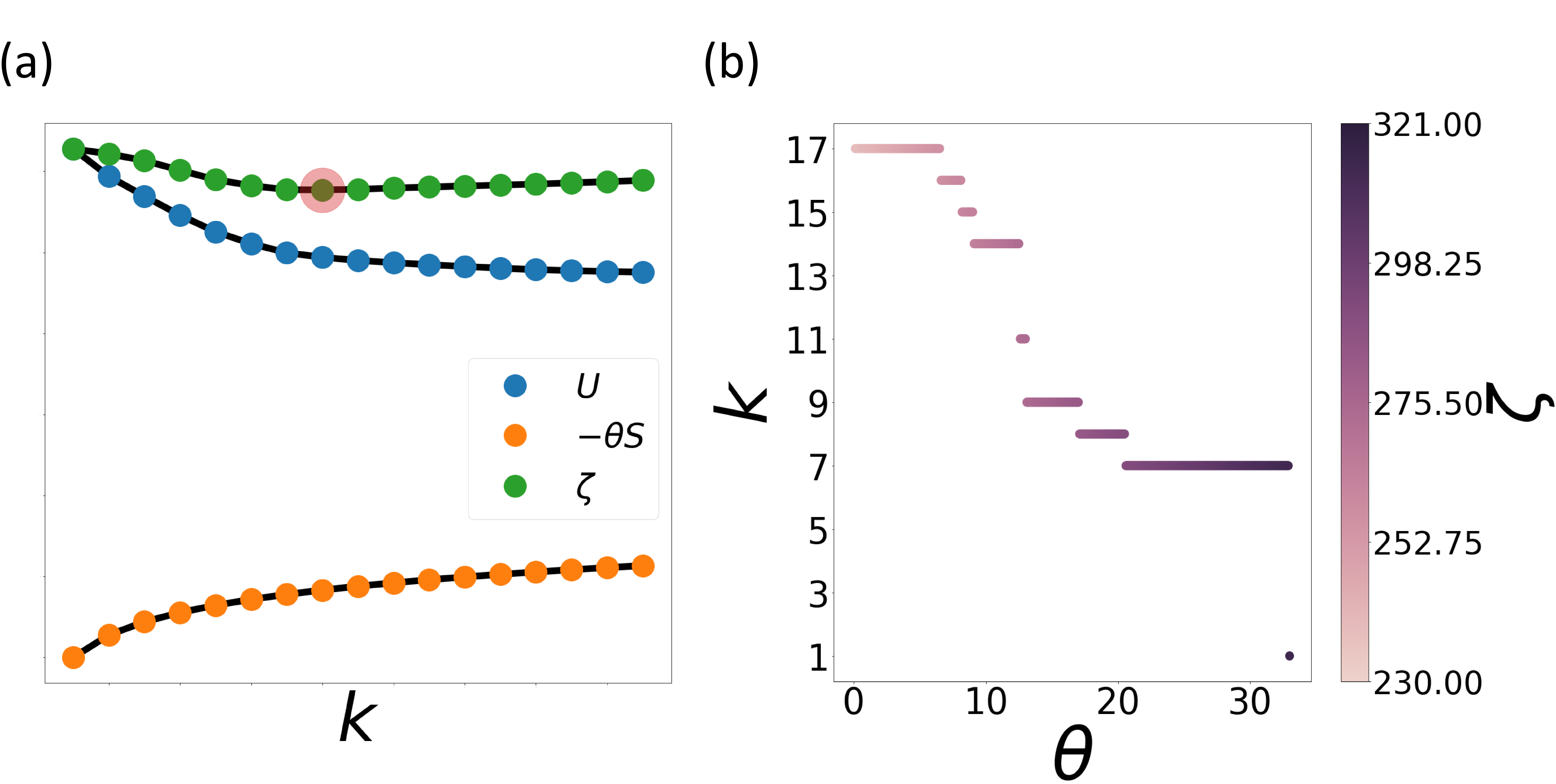
Figure 1: Illustrative example highlighting properties of Interpretation Free Energy $\zeta$, Unfaithfulness $U$, and Simplicity $S$. (a) Strength of $S$ contribution to $\zeta$ can be tuned by the trade-off parameter $\theta$. (b) For a particular problem we construct a phase diagram by plotting $\zeta$ as a function of $k$ and $\theta$. Here, the family of interpretations at $k_{c}=7$ is optimal since it remained stable over the widest range of $\theta$.

Our starting point is some given dataset $\mathcal{X}$ and corresponding predictions $g$ coming from a black-box model. For instance, $\mathcal{X}$ could comprise a collection of chemical compounds, and the prediction $g$ could be if a particular compound is carcinogenic or not. For a particular element $x\in\mathcal{X}$, we seek approximate interpretations or representations $f$ that are as simple as possible while also being as faithful as possible to $g$ in the vicinity of $x$. In order to keep the interpretation simple, we consider linear approximations $f$, which has $k>0$ non-zero coefficients expressed as a linear combination of corresponding human-understandable representative features $\{s_{k}\}$, defined as:

$$f=\Sigma_{j=0}^{k}f_{j}s_{j}$$ (1)

where $f_{j}$ denotes the weight for feature $s_{j}$, and $s_{0}\equiv 1$ denotes identity or null feature. Representative features $\{s_{k}\}$ are typically domain dependent e.g, one-hot encoded superpixels for an image, keywords for text, and standardized values for tabular data. Here, a $k-$coefficient model has $k$ non-zero coefficients out of possible $M$, with the other $M-k$ equaling 0.

Even a linear model with too many non-zero coefficients can become hard to interpret. As such we quantify its simplicity through a Simplicity function $S[f]$ that depends on the number $k$ of non-zero coefficients, defined as:

$$S[f]\equiv S_{k}=-\ln{(k)}$$ (2)

As per Eq. 2, the Simplicity $S$ decreases monotonically with increasing $k>0$. Such a functional form encourages the construction of a sparse linear model. Although other forms of $S$ satisfying the monotonicity property could be used, we found this specific choice of a logarithmic function to be appropriate due to an observation discussed in Appendix VI.1.

Next we introduce an Unfaithfulness function $U[f,d]$ where $d$ represents an appropriate distance metric between the data instance $x$ and some other data point in $\mathcal{X}$. Intuitively, $U$ captures the deviation from the black-box model behaviour within a small neighborhood of interest of the data instance being explained, where different points in the neighborhood are weighted by a distance dependent similarity measure. Given the simplicity and Unfaithfulness functions $S[f]$ and $U[f,d]$, we define the Interpretation Free Energy $\zeta$ as:

$$\zeta[f,d]=U[f,d]-\theta S[f]$$ (3)

Let’s consider a specific problem where $x_{0}$ is a high-dimensional instance for which an explanation is needed for a black-box model prediction $g(x_{0})$. We first generate a neighborhood of $n$ samples $x_{i}$, and associated black-box predictions $g(x_{i})$. Afterwards, a linear, local surrogate model $f$ with $k$ non-zero coefficients $f_{k}$ corresponding to $k$ observed features (Eq. 1) is built by minimizing weighted squares of the residuals between ground-truth $g$ and all possible $k-$coefficient interpretations $f_{k}$ as shown in Eq. (4). Here $\Pi_{i}(x_{0},x_{i})=e^{-d(x_{0},x_{i})^{2}/\sigma^{2}}$ is a Gaussian similarity measure, where $d$ is the distance between instance $x_{0}$ being explained and a neighborhood sample $x_{i}$ (see Sec. II.2 for details). Such a best-fit $k-$coefficient linear model has Unfaithfulness denoted $U_{k}$ which is calculated as follows:

$$U_{k}=\mathop{min}_{f_{k}}{\sum_{i=1}^{n}\Pi_{i}(x_{0},x_{i})\left[g(x_{i})-(\sum_{j=0}^{k}f_{j}s_{ij})\right]^{2}}$$ (4)

With $U$ so defined, it can be seen that increasing $k$ can not increase $U$, as long as the most influential features are added sequentially. Since a model with $k$+1 non-zero coefficients will be less or at best equally unfaithful as a model with $k$ non-zero coefficients defined in Eq. 1. Thus, both $S_{k}$ and $U_{k}$ decrease with increasing $k$, giving us the sought after monotonicity. It should be noted, similar to $S$ the definition of $U$ is also not unique and other forms of $U$ could be chosen (e.g, negatives of the absolute correlation coefficient between constructed surrogate and black-box model predictions as proposed in LIME). However, this framework still holds for other appropriate definitions of $U$, since the observation of diminishing unfaithfulness remains valid for such definitions. We note that our definition of assigning model accuracy using eq. 4, encourages the selection of features with high positive coefficients i.e, features that contribute towards a particular class prediction as opposed to high negative coefficients which increases $U_{k}$ because of the minus ($-$) sign. This is to be contrasted with previous correlation coefficient based model selection schemes, that will likely identify high negative coefficients i.e, features contributing to not in-class prediction along with positives which may make the interpretation difficult in certain applications.

This then gives the Interpretation Free Energy $\zeta$ from Eq. 3 a unique minimum at a critical $k=k_{c}$ with maximal Simplicity and minimum Unfaithfulness as illustrated in Fig. 1. With these definitions of $U$ and $S$ we write down the final expression for the Interpretation Free Energy $\zeta$ as a function of the number of non-zero coefficients $k$ in the interpretation:

$$\zeta(k)=U_{k}-\theta S_{k}\\ =\mathop{min}_{f_{k}}{\sum_{i=1}^{n}\Pi_{i}\left[g(x_{i})-(\sum_{j=0}^{k}f_{j}s_{ij})\right]^{2}}+\theta\ln{(k)}$$ (5)

With this set-up, we now describe a complete protocol for implementing TERP as shown in Algorithm. 1. Our starting points are a high-dimensional data instance $x_{0}\in\mathcal{X}$, and the prediction $g(x_{0})$ from the black-box model $g$.

Next, we follow the framework of local surrogate modelsMolnar (2020) that generate new neighborhood data by randomly perturbing the high-dimensional input space. This has both its pros and cons. The primary advantage over using already existing data used to train the black-box model is that practical high-dimensional input data is typically sparse in nature. Thus it might not do a good job of generating samples from local neighborhood of the data instance being explained. An additional concern could be that the training data used to set up the model is no longer available. At the same time, such local surrogate models can become misleading if the number of features is high. This is because random sampling does not provide a faithful representation of the neighborhood due to the curse of dimensionality. Yet, to keep TERP as model-agnostic, we prefer random sampling as the data generation scheme and perform a second round of neighborhood sampling by perturbing a sub-space of relevant features. Details of constructing this sub-space is provided in Algorithm 1.

Afterwards, all the input features are standardized and a linear model is constructed using ridge regressionHoerl and Kennard (1970) and stochastic gradient descentBottou (2012) optimization scheme. We do not use LASSO regressionTibshirani (2011) typically used in such algorithms to avoid discarding correlated features since in some problems they may still contain useful information. Instead we use a cut-off to discard irrelevant features with coefficient values close to zero and construct a relevant feature sub-space. Time complexity of this step is $O(nk^{2})$. Since, $n$ is the size of the neighborhood and not the size of the training dataset and the feature sub-space is significantly smaller than the entire input space, this step is tractable. Parallel implementation can improve time complexity to $O(nk).$ Finally we employ a forward feature selection algorithm to compute $U$ and identify the most relevant features by tuning $\theta$ as discussed in Algorithm 2.

Algorithm 1 TERP protocol

1:Generate neighborhood data by perturbing input features. Obtain associated black-box predictions.

2:Compute appropriate similarity (Sec. II.2) and construct a linear, surrogate model.

3:Identify relevant features from this model by discarding features with coefficients close to zero.

4:Regenerate neighborhood by perturbing only the identified relevant features for an improved representation, and obtain associated black-box predictions.

5:Implement forward feature selection to identify accurate models by computing $U_{k}$.

6:Obtain optimal interpretation by constructing Interpretation Phase Diagrams (Algorithm 2) and calculating $\zeta$.

II.2 Similarity measure using linear discriminant analysis

As can be seen from the discussion in Sec. II.1, the Interpretation Free Energy $\zeta$ is a functional of the interpretation $f$ as well as a distance measure $d$ which quantifies distance from the specific instance $x$ of data being explained. A key question now is how to appropriately calculate this distance metric $d$, which is crucial for evaluating the similarity measure $\Pi$.

In previous approaches that inspired TERP, particularly LIME,Ribeiro, Singh, and Guestrin (2016) the distance $d$ is calculated through a Euclidean measure in the continuous input feature space of tabular data and through a Cosine measure in the binary representative feature space of image and text data respectively. Computing $d$ based on Euclidean measure has the possibility of producing incorrect similarities if the input space has several correlated or redundant features.Karagiannopoulos et al. (2004); Liang and Zeger (1993) To deal with this problem, TERP computes a one-dimensional (1-d) projection of the neighborhood using linear discriminant analysisIzenman and Izenman (2008) (LDA) for tabular data, which removes redundancy and produces more accurate similarity. LDA generates this 1-d projection by minimizing within class variance and maximizing between class distances. Such a projection encourages formation of two clusters in a 1-d space, corresponding to in-class and not in-class datapoints respectively. Since we are working within a linear regime of the neighborhood, the classes will be well-separated i.e, mean values of the individual classes will not overlap and LDA will be able to produce a meaningful projection. This proposed scheme for computing similarity is not limited to TERP and can be adopted by existing surrogate model approaches e.g, LIME. Advantages of LDA based similarity has been highlighted for a practical application in Sec. IIIA. Fig. 2(e-g).

II.3 Interpretation phase diagram

A natural question to ask pertains to picking the trade-off or temperature-like parameter $\theta$ in Eq. 3. Per our arguments in Sec. II.1 the Interpretation Free Energy $\zeta$ is guaranteed to have a minimum for any choice of $\theta$, naturally the interpretation itself will change with $\theta$. This is again reminiscent of thermodynamics where a system’s equilibrium configuration will in general vary with the temperature and the associated energy-entropy trade-off. At the same time, thermodynamic systems tend to display stable phases over big swaths of control parameters such as the temperature, represented through a phase diagram.Callen (1985) As long as one is in a stable phase region, it does not matter which temperature is picked.

In TERP we draw a direct parallel with the above observation from thermodynamics and propose an Interpretation Phase Diagram. We propose a way to ascertain the stability or robustness of the linear models at different $k$ with respect to the choice of $\theta$ by constructing $\theta$–dependent maps as shown in Fig. 1(b) and outlined in Algorithm 2. A linear model with Interpretation Free Energy minimum at $k=k_{c}$ is stable only if $\zeta_{min}$ does not shift to a different $k=k_{c^{\prime}}$ when $\theta$ is perturbed significantly. This happens when the change in model unfaithfulness is significantly higher/lower for a particular $k=k_{c}$ compared to solutions for others $k$ models and is demonstrated using an illustrative example in Fig. 1. For a stable $k$ coefficient model, we suggest the use of any $\theta$ within the model’s range of stability.

Algorithm 2 Interpretation phase diagram construction

1:Identify the least unfaithful models at different $k$ by computing $U_{k}$ (Algorithm 1).

2:Starting from zero tune $\theta$, and compute $\zeta_{k}$ for these models.

3:Construct a phase diagram as shown in Fig. 1(b) and identify the most stable model at $k=k_{c}$ as the optimal solution.

III Results

In this section, we apply TERP to interpret black-box models applied to a range of domains, including classifiers for physics based simulations, images, and texts. In particular, interpretability approaches for the first class of problems has not seen a systematic implementation yet. Here we interpret autoencoder classification of the conformational states of a peptide molecule observed in MD simulation, convolutional neural network (CNN) predictions for detecting human facial attributes from images, and long short-term memory (LSTM) model predictions for classifying news articles.

III.1 AI-augmented MD method: VAMPnets

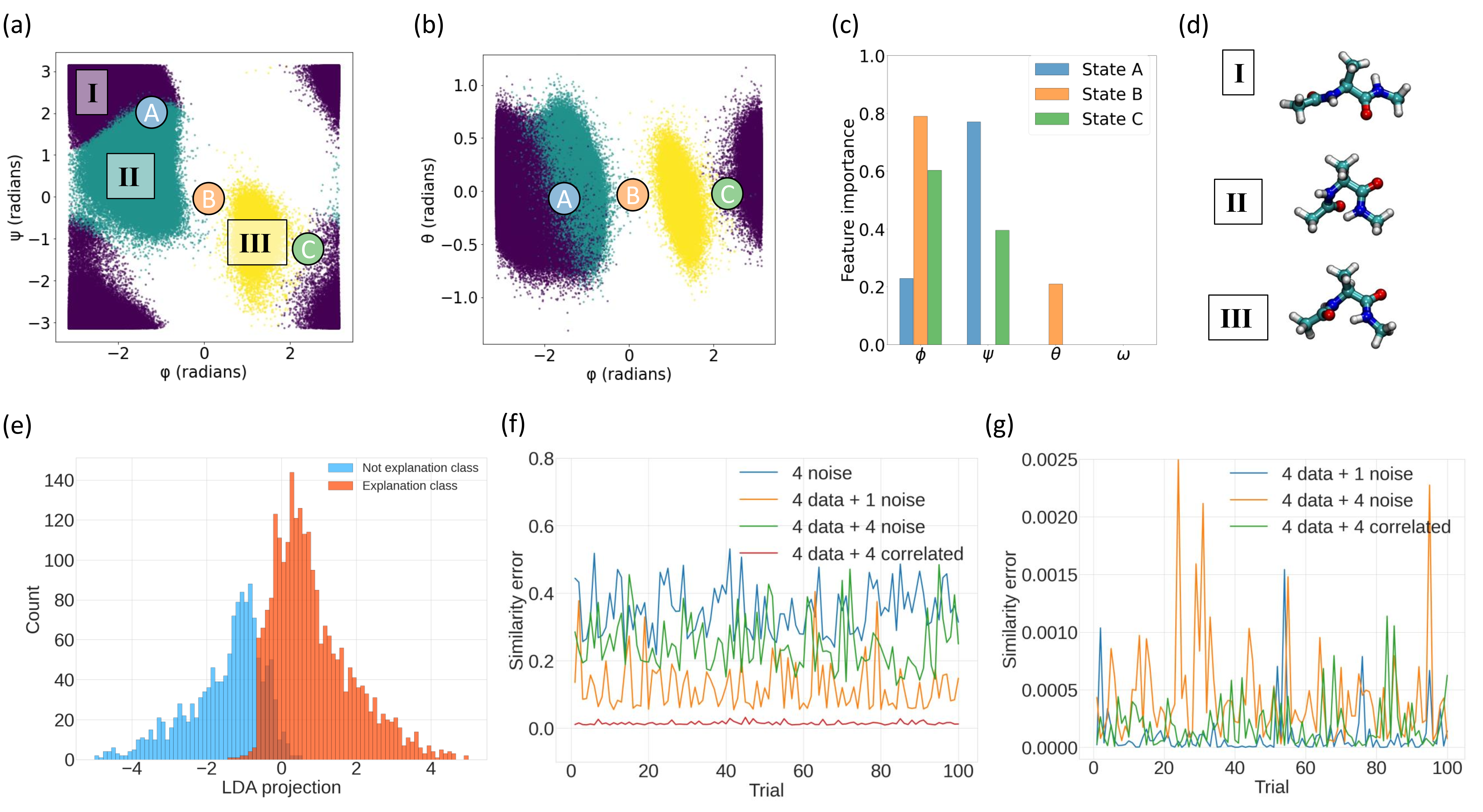
Figure 2: Using TERP to interpret VAMPnet for alanine dipeptide in vacuum. Projected converged states highlighted in three different colors as obtained by VAMPnets along (a) ($\phi,\psi$), and (b) ($\phi,\theta$) dihedral angles. VAMPnets learn the transitions state in this system, three of which were probed using TERP denoted by states A, B, and C. (c) Relative feature importance at A, B, C. (d) Representative conformational states of alanine dipeptide at I, II, III. (e) High dimensional neighborhood data projected onto 1-d using LDA for improved similarity measure. Separation of the two classes indicates meaningful projection. Average similarity error per datapoint for (f) Euclidean, and (g) LDA based similarity respectively. Comparison between (f) and (g) shows minimal error for LDA based similarity, specifically demonstrated for an input space constructed from the four dihedral angles plus one pure noise, four pure noise, and four correlated features with partial noise respectively. The input space for no actual data and four pure noise features in (f) establishes a baseline, showing that the Euclidean similarity will include significant error even when one redundant feature is included. All the calculations were performed in 100 independent trials to appropriately examine the effects.

Variational approach for markov processes (VAMPnets) is a popular technique for analyzing molecular dynamics (MD) trajectories.Mardt et al. (2018) VAMPnets can be used to featurize, transform inputs to a lower dimensional representation, and construct a markov state modelBowman, Pande, and Noé (2013) in an automated manner by maximizing the so called VAMP score. Detailed discussion of VAMPnets theory and parameters are provided in the SI.

In this work, we trained a VAMPnet model on a standard toy system: alanine dipeptide in vacuum. An 8-dimensional input space with sines and cosines of all the dihedral angles $\phi,\psi,\theta,\omega$ was constructed and passed to VAMPnet. VAMPnet was able to identify three metastable states I, II, and III as shown in Fig. 2 (a).

To interpret the VAMPnet model using TERP, we picked three configurations A, B, and C corresponding to three datapoints at the boundaries between the three pairs of states (I, II), (II, III), and (III, I) respectively, thus likely to be configurations from the transition state ensemble for moving between these pairs of states. These three instances were chosen for TERP analysis, with the goal of understanding the reasons behind their classification under respective transition metastable states. Implementing Algorithms 1, and 2, TERP identified $\zeta$ minima at $k_{c}=2$ for all these configurations as highlighted by the corresponding feature importance in Fig. 2 (c). From this figure, we can see that VAMPnet classified B at the boundary between two specific metastable states by considering $\phi$, and $\theta$ dihedral angle, while for configurations A, and C $\phi$, and $\psi$ dihedral angles were taken into account. Additional details are provided in the SI. The feature attributions learned by TERP to explain VAMPnet predictions for this system are in agreement with previous literature,Bolhuis, Dellago, and Chandler (2000) thereby showing that VAMPnet worked here for the right reasons and thus can be trusted.

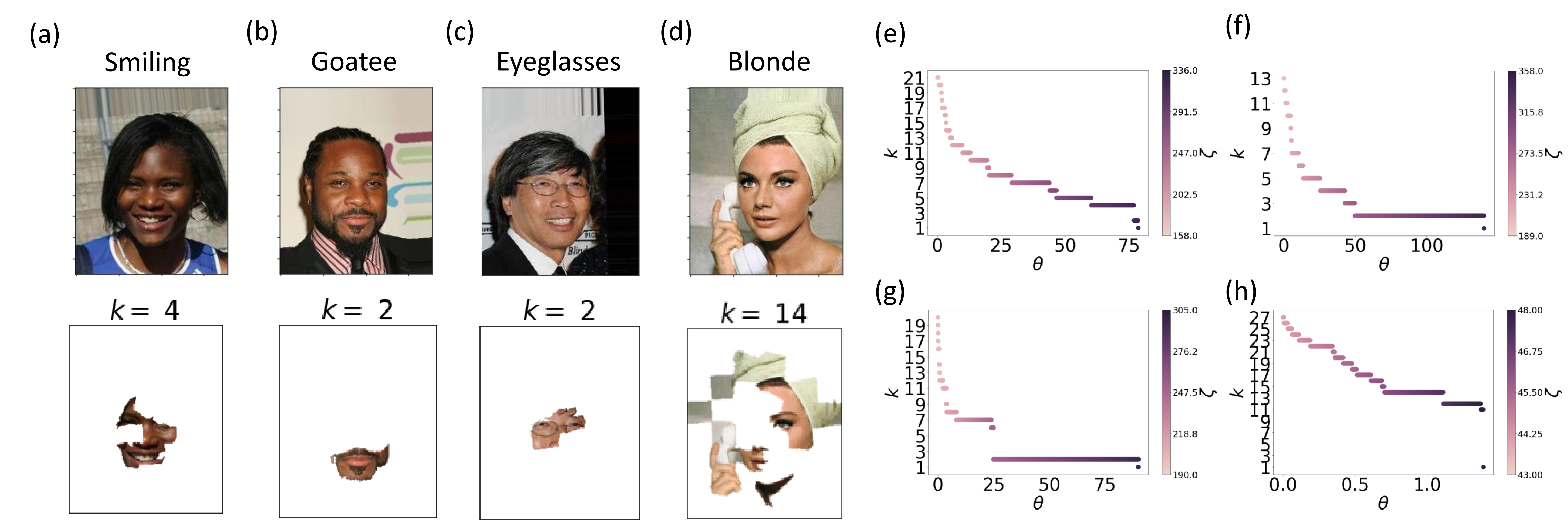
Figure 3: Using TERP to interpret and check reliability of MobileNet model trained on celebA dataset for images not included in the training set. Top rows in (a), (b), (c), and (d) show images classified by MobileNet as ‘smiling’, ‘goatee’, ‘eyeglasses’ and ‘blonde hair’ respectively. Bottoms rows show corresponding free energy optimized explanations generated by TERP. By comparing the figures in the bottom row with the corresponding figures in the top row, it can be seen that the black-box MobileNet model had the right reasons to label the images as ‘smiling’, ‘goatee’, and ‘eyeglasses’ in (a), (b), and (c) respectively. However, for (d) the black-box model prediction of ‘blonde hair’ is clearly wrong. Phase diagrams for (a-d)) are shown in (e-h) respectively.

Next, we demonstrate the implementation of LDA based similarity measure for tabular data. Fig. 2(e) shows that the LDA projection successfully generated two clusters of datapoints belonging to the in-explanation and not in-explanation classes respectively. These well separated clusters help in computing meaningful and improved distance measure $d$. In Figs 2(f,g) we illustrate the robustness of an LDA implementation against noisy and correlated features and compare results with Euclidean similarity implementation. We generate pure white noise by drawing samples from a normal distribution $\mathcal{N}(0,1)$ and generate correlated data by taking $a_{i}x_{i}+b\mathcal{N}(0,1)$ (e.g, $a_{i}=1.0,b=0.2$), where $x_{i}$ are standardized features from the actual data. As shown in Figs. 2(f,g), we construct synthetic neighborhoods by combining actual data from the four dihedral angles and adding one pure noise, four pure noise, four correlated features respectively. Since the synthetic features do not contain any information, their addition should not change similarity. Thus we can compare the robustness of a measure by computing average change in similarity per datapoint squared which we call similarity error, $\Delta\Pi\in[0,1]$ as shown in Eq. 6.

$$\Delta\Pi=\frac{1}{N}\sum_{i=1}^{N}(\Pi_{i}^{o}-\Pi_{i}^{s})^{2}$$ (6)

Here, the superscripts $o$ and $s$ represent similarities corresponding to the original and synthetic datapoints respectively. From Fig. 2(g,h) we can see that LDA based similarity performs significantly better in $100$ independent trials compared to Euclidean similarity. On the other hand, the addition of one pure noise introduces significant similarity error for Euclidean measure. Thus we can conclude that adopting LDA over Euclidean similarity measure will produce significantly improved interpretation.

III.2 Image classification: MobileNets

CNN is a class of AI that has become very popular and is constructed from a deep, non-fully connected feed forward artificial neural network (ANN). Because of their unique architecture, CNNs are efficient in analyzing data with local correlations and have numerous applications in computer vision and in other fields.Traore, Kamsu-Foguem, and Tangara (2018); Giménez, Palanca, and Botti (2020); Pelletier, Webb, and Petitjean (2019) Per construction, CNNs are black-box models and because of their practical usage, it is desirable to employ an interpretation scheme to validate their predictions before deploying them.

In this work, we examine MobileNetsHoward et al. (2017), a particular CNN implementation for image recognition that is suitable for mobile devices due to it being architecturally light-weight. We trained a MobileNet model using the publicly available large-scale CelebFaces Attributes (CelebA)Liu et al. (2018) dataset to learn $21$ features from $141,820$ Human facial images. Details of the architecture and training procedure are provided in the SI.

Fig. 3 shows results from having employed TERP to explain feature predictions from four images that were not present in the training data. For this purpose, every image was divided into superpixels by using the SLIC image segmentation algorithm.Achanta et al. (2010) These superpixels are then perturbed to generate neighborhood data based on which a linear, interpretable model is constructed by minimizing the Interpretation Free Energy in Eq. 5. We can see from Fig. 3 (a), (b), and (c) respectively that for the attributes ‘smiling’, ‘goatee’, and ‘eyeglasses’, the black-box model made predictions based on reasons that a human reader of this manuscript would perceive as justified. However, for Fig. 3 (d), the black-box model predicted the attribute ‘blonde hair’, which is clearly wrong. The relevant superpixels for this prediction as identified by TERP indicates that the reasons behind this black-box prediction had nothing to do with hair or its color. For these four images, TERP generates the Interpretation Free Energy $\zeta$ minima at four different $k_{c}=4,2,2,14$ as shown in Fig. 3 (e), (f), (g), and (h) respectively. From these Interpretation Phase Diagrams it can be observed that the surrogate models constructed at $k_{c}$ are the most stable in terms of temperature $\theta$, indicating that the model achieved highest improvement at these $k_{c}$. TERP parameters for these four explanations are provided in SI.

III.3 Text classification: Attention-based Bidirectional Long Short-Term Memory (Att-BLSTM)

Classification tasks in natural language processing (NLP) involve identifying semantic relations between units appearing at distant locations of in a block of text. This challenging problem is known as relation classification and models based on long short-term memory (LSTM)Yu et al. (2019), gated recurrent unit (GRU)Chung et al. (2014), transformersVaswani et al. (2017) have been very successful in addressing such problems. In this work, we look at the widely used attention-based bidirectional long short-term memoryZhou et al. (2016) (AttBLSTM) classifier and apply TERP to interpret its predictions.

First, we trained an AttBLSTM model on Antonio Gulli’s (AG’s) news corpusGulli (2005), which is a large collection of more than $1$ million news articles curated from more than $2,000$ news sources. The labels associated with each news article in the dataset indicates the section of the news source (e.g, World, Sports, Business, or Science and technology) that the news was published in. Afterwards, we employed the trained model and obtained predictions for each of the news stories published in a special edition of Nature News (Nature’s biggest news stories of 2022)nat (2022) which was not included in the training data.

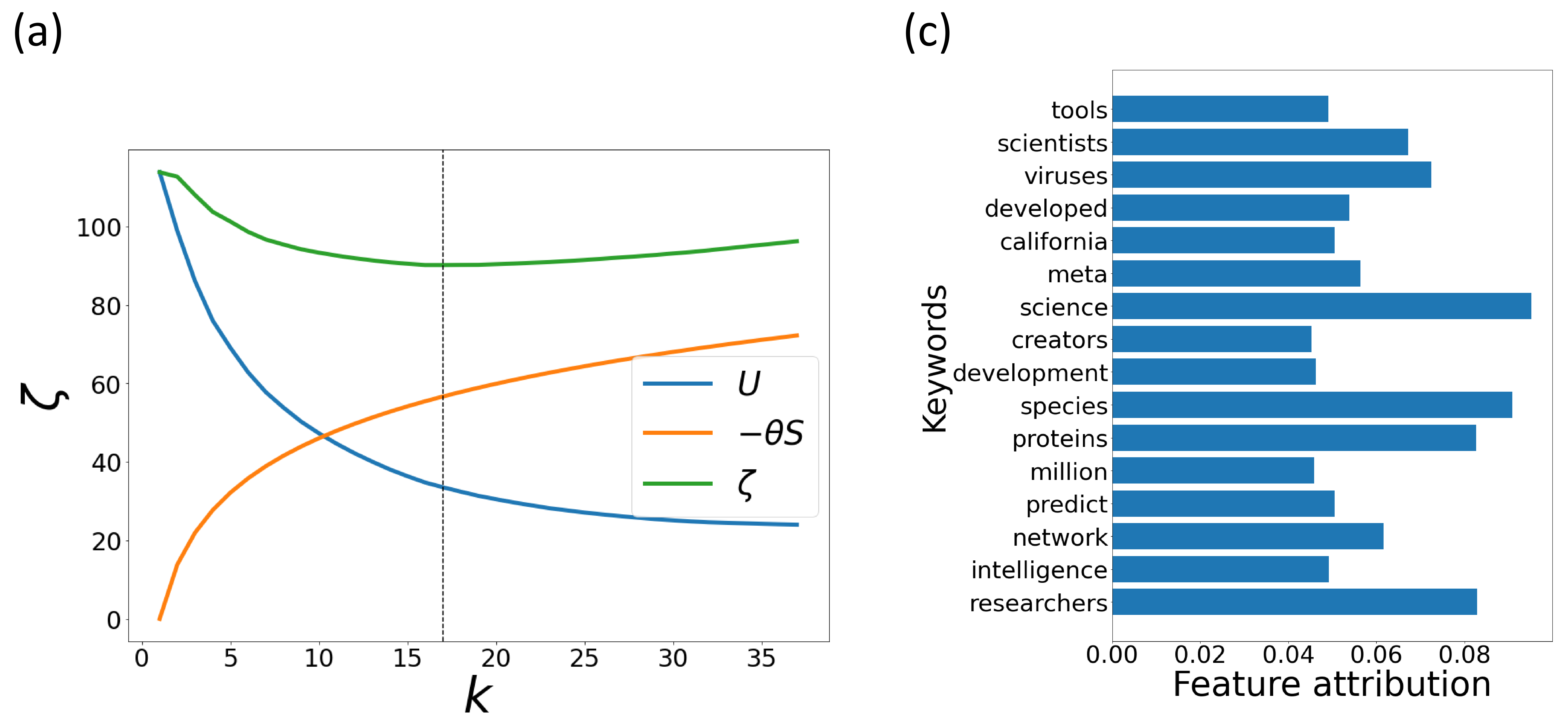
Figure 4: Using TERP to interpret and check reliability of AttBLSTM model trained on AG’s news corpus to predict the news story titled ”AI predicts protein structures”. (a) $\zeta$ vs. $k$ plot showing $k_{c}=16$ at $\theta=20$, (b) relative feature attribution for the most relevant 16 features for prediction as identified by TERP.

In in Fig. 4 we highlight the results for one out of the ten news stories titled “AI predicts protein structures”. The AttBLSTM classifier predicted that the news is about Science and Technology and the most influential keywords for this prediction have been identified by TERP in Fig. 4(b). Interestingly, AttBLSTM makes its prediction not from a few keywords but from a collection of keywords which is possibly the reason behind its success. Interesting results about four other news stories, for some of which AttBLSTM fails to make a correct prediction have been provided in the SI. Here TERP based interpretation gives confidence that Att-BLSTM was able to identify relevant semantic relations and classified the news story for the correct reasons, since from Fig. 4(b) we see that almost all of the influential keywords are about Science and Technology including the keyword ”Science” itself having the highest influence.

IV Discussion

The use of AI-based black-box models has now become a staple feature across domains as they can be deployed without any need for a fundamental understanding of the governing processes at work. This strength is however their weakness too, as it leads to questions about whether an AI model can be trusted and how one should proceed about deriving the meaning of any AI based model. In this work, we established a thermodynamics inspired framework for generating interpretable representations of complex black-box models, wherein the optimal representation was expressed as one that minimizes unfaithfulness to the ground truth model, while still staying as simple as possible. This trade-off was quantified through the concept of an Interpretation Free Energy which has simple but useful mathematical properties guaranteeing the existence of a global minima. We demonstrated the use of this approach on different problems using AI, such as classifying images, texts and tablular data. Numerous approaches have been proposed to tackle this problem Ribeiro, Singh, and Guestrin (2016); Fisher, Rudin, and Dominici (2019); Lundberg and Lee (2017); Sundararajan, Taly, and Yan (2017); Wachter, Mittelstadt, and Russell (2017), however very few with the notable exception of Ref. Wellawatte, Seshadri, and White, 2022; Kikutsuji et al., 2022; Fleetwood et al., 2020 have been used to explain molecular simulations. Finally, we believe that arguably TERP is one of the first applications of interpretability schemes to AI-augmented molecular dynamics, which is a rapidly burgeoning sub-discipline in its own right. Since molecular sciences are being employed to discover chemical reaction pathways,Yang et al. (2017) understand disease mechanisms,Hollingsworth and Dror (2018) design effective drugsZhao and Caflisch (2015) and many other applications, an incorrect black-box analysis can have severe financial and public health consequences in addition to providing an incorrect understanding of these phenomena. TERP should provide practitioners of molecular sciences a way to interpret these black-box models on a footing made rigorous through simple yet powerful parallels with the field of thermodynamics.

Code for TERP is available at github.com/tiwarylab/TERP.

V Acknowledgments

This work was supported by the National Science Foundation, grant no. CHE-2044165. The authors thank Dr. Eric Beyerle for insightful discussions. The authors also thank Deepthought2, MARCC, and XSEDE (projects CHE180007P and CHE180027P) for the computational resources used in this work.

VI Appendices

VI.1 Rationale for choice of Simplicity Function

Here we note a key observation that for practical problems, the decrease in Unfaithfulness becomes less prominent as $k$ is increased and eventually becomes zero if the most relevant features are added sequentially to the surrogate model. In other words, only a handful of features typically have the most influence in black-box model prediction. Due to this property of $U$, we choose a logarithmic definition of $S$ since it balances $U$ in a stable manner. Effectively, at a particular $\theta$, $\zeta_{min}$ is achieved at $k=k_{c}$ when decrease in $U$ becomes worse compared to a logarithmic decrease.

References

References

- Dhar (2013) V. Dhar, “Data science and prediction,” Communications of the ACM 56, 64–73 (2013).
- Shalev-Shwartz and Ben-David (2014) S. Shalev-Shwartz and S. Ben-David, Understanding machine learning: From theory to algorithms (Cambridge university press, 2014).
- LeCun, Bengio, and Hinton (2015) Y. LeCun, Y. Bengio, and G. Hinton, “Deep learning,” nature 521, 436–444 (2015).
- Davies et al. (2021) A. Davies, P. Veličković, L. Buesing, S. Blackwell, D. Zheng, N. Tomašev, R. Tanburn, P. Battaglia, C. Blundell, A. Juhász, et al., “Advancing mathematics by guiding human intuition with ai,” Nature 600, 70–74 (2021).
- Carleo et al. (2019) G. Carleo, I. Cirac, K. Cranmer, L. Daudet, M. Schuld, N. Tishby, L. Vogt-Maranto, and L. Zdeborová, “Machine learning and the physical sciences,” Reviews of Modern Physics 91, 045002 (2019).
- Mater and Coote (2019) A. C. Mater and M. L. Coote, “Deep learning in chemistry,” Journal of chemical information and modeling 59, 2545–2559 (2019).
- Hamet and Tremblay (2017) P. Hamet and J. Tremblay, “Artificial intelligence in medicine,” Metabolism 69, S36–S40 (2017).
- Baldi and Brunak (2001) P. Baldi and S. Brunak, Bioinformatics: the machine learning approach (MIT press, 2001).
- Brunton and Kutz (2022) S. L. Brunton and J. N. Kutz, Data-driven science and engineering: Machine learning, dynamical systems, and control (Cambridge University Press, 2022).
- Loyola-Gonzalez (2019) O. Loyola-Gonzalez, “Black-box vs. white-box: Understanding their advantages and weaknesses from a practical point of view,” IEEE Access 7, 154096–154113 (2019).
- Rudin (2019) C. Rudin, “Stop explaining black box machine learning models for high stakes decisions and use interpretable models instead,” Nature Machine Intelligence 1, 206–215 (2019).
- Callen (1985) H. B. Callen, “Thermodynamics and an introduction to thermostatistics,” (1985).
- Kumar and Minz (2014) V. Kumar and S. Minz, “Feature selection: a literature review,” SmartCR 4, 211–229 (2014).
- Ribeiro, Singh, and Guestrin (2016) M. T. Ribeiro, S. Singh, and C. Guestrin, “” why should i trust you?” explaining the predictions of any classifier,” in Proceedings of the 22nd ACM SIGKDD international conference on knowledge discovery and data mining (2016) pp. 1135–1144.
- Fisher, Rudin, and Dominici (2019) A. Fisher, C. Rudin, and F. Dominici, “All models are wrong, but many are useful: Learning a variable’s importance by studying an entire class of prediction models simultaneously.” J. Mach. Learn. Res. 20, 1–81 (2019).
- Lundberg and Lee (2017) S. M. Lundberg and S.-I. Lee, “A unified approach to interpreting model predictions,” Advances in neural information processing systems 30 (2017).
- Gupta, Kulkarni, and Mukherjee (2021) A. Gupta, M. Kulkarni, and A. Mukherjee, “Accurate prediction of b-form/a-form dna conformation propensity from primary sequence: A machine learning and free energy handshake,” Patterns 2, 100329 (2021).
- Sundararajan, Taly, and Yan (2017) M. Sundararajan, A. Taly, and Q. Yan, “Axiomatic attribution for deep networks,” in International conference on machine learning (PMLR, 2017) pp. 3319–3328.
- Wachter, Mittelstadt, and Russell (2017) S. Wachter, B. Mittelstadt, and C. Russell, “Counterfactual explanations without opening the black box: Automated decisions and the gdpr,” Harv. JL & Tech. 31, 841 (2017).
- Wellawatte, Seshadri, and White (2022) G. P. Wellawatte, A. Seshadri, and A. D. White, “Model agnostic generation of counterfactual explanations for molecules,” Chemical science 13, 3697–3705 (2022).
- Mardt et al. (2018) A. Mardt, L. Pasquali, H. Wu, and F. Noé, “Vampnets for deep learning of molecular kinetics,” Nature communications 9, 1–11 (2018).
- Howard et al. (2017) A. G. Howard, M. Zhu, B. Chen, D. Kalenichenko, W. Wang, T. Weyand, M. Andreetto, and H. Adam, “Mobilenets: Efficient convolutional neural networks for mobile vision applications,” (2017).
- Zhou et al. (2016) P. Zhou, W. Shi, J. Tian, Z. Qi, B. Li, H. Hao, and B. Xu, “Attention-based bidirectional long short-term memory networks for relation classification,” in Proceedings of the 54th annual meeting of the association for computational linguistics (volume 2: Short papers) (2016) pp. 207–212.
- Frenkel and Smit (2001) D. Frenkel and B. Smit, Understanding molecular simulation: from algorithms to applications, Vol. 1 (Elsevier, 2001).
- Doerr et al. (2021) S. Doerr, M. Majewski, A. Pérez, A. Kramer, C. Clementi, F. Noe, T. Giorgino, and G. De Fabritiis, “Torchmd: A deep learning framework for molecular simulations,” Journal of chemical theory and computation 17, 2355–2363 (2021).
- Han et al. (2017) J. Han, L. Zhang, R. Car, et al., “Deep potential: A general representation of a many-body potential energy surface,” arXiv preprint arXiv:1707.01478 (2017).
- Gao et al. (2020) X. Gao, F. Ramezanghorbani, O. Isayev, J. S. Smith, and A. E. Roitberg, “Torchani: a free and open source pytorch-based deep learning implementation of the ani neural network potentials,” Journal of chemical information and modeling 60, 3408–3415 (2020).
- Wang and Tiwary (2021) D. Wang and P. Tiwary, “State predictive information bottleneck,” The Journal of Chemical Physics 154, 134111 (2021).
- Ma and Dinner (2005) A. Ma and A. R. Dinner, “Automatic method for identifying reaction coordinates in complex systems,” The Journal of Physical Chemistry B 109, 6769–6779 (2005).
- Wang, Ribeiro, and Tiwary (2020) Y. Wang, J. M. L. Ribeiro, and P. Tiwary, “Machine learning approaches for analyzing and enhancing molecular dynamics simulations,” Current opinion in structural biology 61, 139–145 (2020).
- Beyerle, Mehdi, and Tiwary (2022) E. R. Beyerle, S. Mehdi, and P. Tiwary, “Quantifying energetic and entropic pathways in molecular systems,” The Journal of Physical Chemistry B (2022).
- Ribeiro et al. (2018) J. M. L. Ribeiro, P. Bravo, Y. Wang, and P. Tiwary, “Reweighted autoencoded variational bayes for enhanced sampling (rave),” The Journal of chemical physics 149, 072301 (2018).
- Vanden-Eijnden (2014) E. Vanden-Eijnden, “Transition path theory,” An introduction to Markov state models and their application to long timescale molecular simulation , 91–100 (2014).
- Smith et al. (2020) Z. Smith, P. Ravindra, Y. Wang, R. Cooley, and P. Tiwary, “Discovering protein conformational flexibility through artificial-intelligence-aided molecular dynamics,” The Journal of Physical Chemistry B 124, 8221–8229 (2020).
- Molnar (2020) C. Molnar, Interpretable machine learning (Lulu. com, 2020).
- Hoerl and Kennard (1970) A. E. Hoerl and R. W. Kennard, “Ridge regression: applications to nonorthogonal problems,” Technometrics 12, 69–82 (1970).
- Bottou (2012) L. Bottou, “Stochastic gradient descent tricks,” in Neural networks: Tricks of the trade (Springer, 2012) pp. 421–436.
- Tibshirani (2011) R. Tibshirani, “Regression shrinkage and selection via the lasso: a retrospective,” Journal of the Royal Statistical Society: Series B (Statistical Methodology) 73, 273–282 (2011).
- Karagiannopoulos et al. (2004) M. Karagiannopoulos, D. Anyfantis, S. Kotsiantis, and P. Pintelas, “Feature selection for regression problems,” Educational Software Development Laboratory, Department of Mathematics, University of Patras, Greece (2004).
- Liang and Zeger (1993) K.-Y. Liang and S. L. Zeger, “Regression analysis for correlated data,” Annual review of public health 14, 43–68 (1993).
- Izenman and Izenman (2008) A. J. Izenman and A. J. Izenman, “Linear discriminant analysis,” Modern multivariate statistical techniques: regression, classification, and manifold learning , 237–280 (2008).
- Bowman, Pande, and Noé (2013) G. R. Bowman, V. S. Pande, and F. Noé, An introduction to Markov state models and their application to long timescale molecular simulation, Vol. 797 (Springer Science & Business Media, 2013).
- Bolhuis, Dellago, and Chandler (2000) P. G. Bolhuis, C. Dellago, and D. Chandler, “Reaction coordinates of biomolecular isomerization,” Proceedings of the National Academy of Sciences 97, 5877–5882 (2000).
- Traore, Kamsu-Foguem, and Tangara (2018) B. B. Traore, B. Kamsu-Foguem, and F. Tangara, “Deep convolution neural network for image recognition,” Ecological Informatics 48, 257–268 (2018).
- Giménez, Palanca, and Botti (2020) M. Giménez, J. Palanca, and V. Botti, “Semantic-based padding in convolutional neural networks for improving the performance in natural language processing. a case of study in sentiment analysis,” Neurocomputing 378, 315–323 (2020).
- Pelletier, Webb, and Petitjean (2019) C. Pelletier, G. I. Webb, and F. Petitjean, “Temporal convolutional neural network for the classification of satellite image time series,” Remote Sensing 11, 523 (2019).
- Liu et al. (2018) Z. Liu, P. Luo, X. Wang, and X. Tang, “Large-scale celebfaces attributes (celeba) dataset,” Retrieved August 15, 11 (2018).
- Achanta et al. (2010) R. Achanta, A. Shaji, K. Smith, A. Lucchi, P. Fua, and S. Süsstrunk, “Slic superpixels,” Tech. Rep. (2010).
- Yu et al. (2019) Y. Yu, X. Si, C. Hu, and J. Zhang, “A review of recurrent neural networks: Lstm cells and network architectures,” Neural computation 31, 1235–1270 (2019).
- Chung et al. (2014) J. Chung, C. Gulcehre, K. Cho, and Y. Bengio, “Empirical evaluation of gated recurrent neural networks on sequence modeling,” arXiv preprint arXiv:1412.3555 (2014).
- Vaswani et al. (2017) A. Vaswani, N. Shazeer, N. Parmar, J. Uszkoreit, L. Jones, A. N. Gomez, Ł. Kaiser, and I. Polosukhin, “Attention is all you need,” Advances in neural information processing systems 30 (2017).
- Gulli (2005) A. Gulli, “The anatomy of a news search engine,” in Special interest tracks and posters of the 14th international conference on World Wide Web (2005) pp. 880–881.
- nat (2022) “Nature’s biggest news stories of 2022,” (2022).
- Kikutsuji et al. (2022) T. Kikutsuji, Y. Mori, K.-i. Okazaki, T. Mori, K. Kim, and N. Matubayasi, “Explaining reaction coordinates of alanine dipeptide isomerization obtained from deep neural networks using explainable artificial intelligence (xai),” The Journal of Chemical Physics 156, 154108 (2022).
- Fleetwood et al. (2020) O. Fleetwood, M. A. Kasimova, A. M. Westerlund, and L. Delemotte, “Molecular insights from conformational ensembles via machine learning,” Biophysical Journal 118, 765–780 (2020).
- Yang et al. (2017) M. Yang, J. Zou, G. Wang, and S. Li, “Automatic reaction pathway search via combined molecular dynamics and coordinate driving method,” The Journal of Physical Chemistry A 121, 1351–1361 (2017).
- Hollingsworth and Dror (2018) S. A. Hollingsworth and R. O. Dror, “Molecular dynamics simulation for all,” Neuron 99, 1129–1143 (2018).
- Zhao and Caflisch (2015) H. Zhao and A. Caflisch, “Molecular dynamics in drug design,” European journal of medicinal chemistry 91, 4–14 (2015).