Canonical tessellations
of decorated hyperbolic surfaces

Abstract.

A decoration of a hyperbolic surface of finite type is a choice of circle, horocycle or hypercycle about each cone-point, cusp or flare of the surface, respectively. In this article we show that a decoration induces a unique canonical tessellation and dual decomposition of the underlying surface. They are analogues of the weighted Delaunay tessellation and Voronoi decomposition in the Euclidean plane. We develop a characterisation in terms of the hyperbolic geometric equivalents of Delaunay’s empty-discs and Laguerre’s tangent-distance, also known as power-distance. Furthermore, the relation between the tessellations and convex hulls in Minkowski space is presented, generalising the Epstein-Penner convex hull construction. This relation allows us to extend Weeks’ flip algorithm to the case of decorated finite type hyperbolic surfaces. Finally, we give a simple description of the configuration space of decorations and show that any fixed hyperbolic surface only admits a finite number of combinatorially different canonical tessellations.

1. Introduction

It is commonly known that one can associate to a finite set of points $V$ in the Euclidean plane two dual combinatorial structures: the Delaunay tessellation and the Voronoi decomposition. The former is a tessellation of $\operatorname{conv}(V)$ with vertex set $V$ such that faces are given as the convex hulls of vertices on the boundaries of empty discs, i.e., discs which contain no point of $V$ in their interiors. The latter is a decomposition of the Euclidean plane into regions, each consisting of all points closest to one of the points in $V$, respectively.

The study of Voronoi decompositions has a long history. It dates back at least to L. Dirichlet’s analysis of fundamental domains of $2$- and $3$-dimensional Euclidean lattices in 1850 [Dirichlet50]. The analogous considerations of H. Poincaré for Fuchsian groups acting on the hyperbolic plane are almost as old [Poincare82]. The first general results in $N$-dimensions are due to G. Voronoï [Voronoi08]. His student B. Delaunay introduced the dual approach via empty spheres [Delaunay34]. The classical motivations for studying these tessellations and there generalisations, i.e., weighed Delaunay tessellations and weighted Voronoi decompositions, are diverse. They range form number-theoretic considerations in the reduction theory of quadratic forms [Dirichlet50][Voronoi08][Delaunay34], over questions in surface theory [Poincare82] to statics and kinematics of frameworks and the analysis of combinatorics of convex polyhedra [Izmestiev19][EricksonLin21].

Since the 1980s canonical tessellations, i.e., weighted Delaunay tessellations, of hyperbolic cusp surfaces play an important role in the analysis of Teichmüller and moduli spaces [Harer88][Penner12]. One approach to these tessellations considers level sets of intrinsic “polar coordinates” which can be introduced about each cusp of the surface. It is due to ideas of W. Thurston and was worked out by B. Bowditch, D. Epstein and L. Mosher [Harer88]*Chapter 2, §3[BowditchEpstein88]. Another approach introduced by D. Epstein and R. Penner uses affine lifts to convex hulls in Minkowski-space [EpsteinPenner88], the Epstein-Penner convex hull construction. Subsequently, the latter approach was successfully applied to closed hyperbolic surfaces with a finite number of distinguished points [NaatanenPenner91], compact hyperbolic surfaces with boundaries [Ushijima99] and projective manifolds with radial ends [CooperLong13]. The convex hull construction gives rise to an explicit method to compute the weighted Delaunay tessellations, the flip algorithm. It was originally explored by J. Weeks for decorated hyperbolic cusp surfaces [Weeks93] and recently extended to projective surfaces by S. Tillmann and S. Wong [TillmannWong16].

Weighted Delaunay tessellations of closed hyperbolic surfaces and surfaces with singular Euclidean structure (PL-surfaces) are closely related to $3$-dimensional hyperbolic polyhedra. They can be characterised as critical points of certain “energy-functionals” related to the volumes of these polyhedra [Leibon02][Rivin94][Springborn08]. Conversely, weighted Delaunay tessellations have proven to be a valuable tool for finding variational methods for the polyhedral realisation of hyperbolic cusp surfaces [Springborn20][Prosanov20] (see [Fillastre08] for an overview of the general problem).

Finally, weighted Delaunay tessellations and Voronoi decompositions are interesting for applications (see [BogdanovEtAl14][Edelsbrunner00][ImaiEtAl85] and references therein). In particular, there is a flip algorithm to compute Delaunay triangulations of PL-surfaces [IndermitteEtAl01]. These can be used to define a discrete notion of intrinsic Laplace-Beltrami operator [BobenkoSpringborn07]. Furthermore, there are surprising connections between discrete conformal equivalence and decorated hyperbolic cusp surfaces [BobenkoEtAl15]. Their weighted Delaunay tessellations play an important role in the theoretical proof of the discrete uniformization theorem [GuEtAl18a][GuEtAl18b] (see also [Springborn20]). Additionally, they are necessary to ensure optimal results when computing discrete conformal maps [GillespieEtAl21].

1.1. Statements of the article

In this article we are going to define and analyse weighted Delaunay tessellations and Voronoi decompositions on decorated hyperbolic surfaces of finite type. Our constructions contain the results about tessellations obtained in [BowditchEpstein88][EpsteinPenner88][NaatanenPenner91] [Ushijima99][Weeks93] as special cases. Another important class of examples are hyperbolic surfaces corresponding to the quotients of the hyperbolic plane by a finitely generated, non-elementary Fuchsian groups (see Figure 1 and Example 3.1).

Figure 1. A tessellation of the hyperbolic plane corresponding to a weighted Delaunay triangulation (solid lines) and its dual weighted Voronoi decomposition (dashed lines) of a decorated hyperbolic surface. The surface can be obtained by identifying the boundary edges of a fundamental domain (darker shaded) as indicated by arrows. It is homeomorphic to a twice punctured sphere and has a cone-point (striped), cusp (chequered) and flare (solid). The identifications correspond to the action of a Fuchsian group.

Informally speaking, a hyperbolic surface of finite type consists of a surface $\Sigma$ which is homeomorphic to a closed orientable surface $\bar{\Sigma}$ minus a finite set of points $V_{0}\cup V_{1}$ endowed with a complete hyperbolic path-metric $\operatorname{dist}_{\Sigma}$ which possesses a finite number of cone-points $V_{-1}\subset\Sigma$, ends of finite area $V_{0}$ (cusps) and infinite area ends $V_{1}$ (flares). Each “point” in $V\coloneq V_{-1}\cup V_{0}\cup V_{1}$ is decorated with a hyperbolic cycle of the respective type, i.e., a circle, horocycle or hypercycle.

In Theorem 3.4 we prove the existence and uniqueness of weighted Delaunay tessellations. They are defined using properly immersed discs, the analogue of B. Delaunay’s empty discs for decorated hyperbolic surfaces. The corresponding results about weighted Voronoi decompositions are contained in Theorem 3.9. Their $2$-cells consist of all points of $\Sigma$ closest to one of the decorated vertices in $V$ measured in the modified tangent distance, respectively. The distance is an analogue of E. Laguerre’s tangent-distance, also known as “power distance” in the Euclidean plane (see [Blaschke29]). Our construction generalises the approach of L. Mosher, B. Bowditch and D. Epstein. Theorem 3.12 reveals the connections between weighted Delaunay tessellations and Voronoi decompositions. The flip algorithm is discussed in Theorem 3.14. We prove that for all proper decorations (see section 3.3) a weighted Delaunay triangulation of $\Sigma$ can be computed from an arbitrary geodesic triangulation in finite time. All steps to actually implement the algorithm are discussed. For the analysis of the flip algorithm we introduce support functions, i.e., the local “scaling offsets” from the one-sheeted hyperboloid, on the surface (compare to [Fillastre13]). If the hyperbolic surface corresponds to a Fuchsian group, the support function associated to a weighted Delaunay triangulation induces a convex hull in Minkowski-space (Corollary 3.16). This is a direct generalisation of the Epstein-Penner convex hull construction to all finitely generated, non-elementary Fuchsian groups. Finally, Theorem 4.3 identifies the configuration space of proper decorations as a convex, connected subset of $\mathbb{R}_{>0}^{V}$ and discusses the dependence of the combinatorics of weighted Delaunay tessellations on the decoration. In particular, we prove a generalisation of “Akiyoshi’s compactification” [Akiyoshi00][GuEtAl18a]*Appendix, that is, we prove that any fixed hyperbolic surface of finite type only admits a finite number of combinatorially different weighted Delaunay tessellations. Moreover, we show that weighted Delaunay tessellations induce a decomposition of the configuration space into convex polyhedral cones. This is an analogue of the classical secondary fan associated to a finite number of points in the Euclidean plane [GelfandEtAl94]*Chapter 7[DeLoeraEtAl10]*Chapter 5.

We highlight that the main methods of this article, namely, properly immersed discs, tangent-distances and support functions, are intrinsic in nature. That is, they only depend on the metric of the surface and the given decoration. In contrast most other approaches like the classical Epstein-Penner convex hull construction or the “empty discs” utilised in [DespreEtAl20] rely on the existence of (metric) covers of the surface by the hyperbolic plane. Notable exceptions are the approach by B. Bowditch, D. Epstein and L. Mosher for hyperbolic cusp surfaces and the “empty immersed discs” A. Bobenko and B. Springborn considered for PL-surfaces. It is important to notice that for the objects of interest of this article, i.e., canonical tessellations of finite type hyperbolic surfaces, (metric) covers by the hyperbolic plane do in general not exist. Thus a classical Epstein-Penner convex hull construction is not feasible.

1.2. Outline of the article

We begin our expositions with an introduction to the local geometry of hyperbolic cycles and their associated polygons in section 2. The main aim is to derive relations between hyperbolic cycles, hyperbolic polygons and the hyperbolic analogue of E. Laguerre’s tangent-distance. This will lead us to a generalisation of J. Weeks’ tilt formula [Weeks93, SakumaWeeks95].

In the next section 3 we are turning our attention to hyperbolic surfaces of finite type. After collecting some properties of these surfaces we introduce and analyse weighted Delaunay tessellations and Voronoi decompositions. We close this section with an analysis of the flip algorithm and a generalisation of the Epstein-Penner convex hull construction to decorated hyperbolic surfaces.

The last section 4 is about characterising the configuration space of decorations of a fixed hyperbolic surface of finite type. Furthermore, we consider some explicit examples.

1.3. Open questions

Using the convex hull construction, R. Penner introduced a mapping class group invariant cell decomposition of the decorated Teichmüller space of hyperbolic cusp surfaces [Penner87, Penner12]. A. Ushijima presented a similar construction for Teichmüller spaces of compact surfaces with boundary [Ushijima99]. But his constructions do not cover decorations of these surfaces. Actually, in light of this article, we see that A. Ushijima implicitly prescribes a constant radius decoration for all surfaces. It remains the question whether his decompositions extend to decorated Teichüller spaces exhibiting equal properties to the case of hyperbolic cusp surfaces.

Independently of these questions the structure of the configuration space of decorations for a fixed surface remains interesting on its own. M. Joswig, R. Löwe and B. Springborn showed that the notions of secondary fan and polyhedron can be defined for decorated hyperbolic cusp surfaces [JoswigEtAl20]. Our Theorem 4.3 provides the existence of secondary fans for the more general class of finite type hyperbolic surfaces. Their secondary polyhedra still remain to be investigated.

The algorithmic aspects of finding weighted Delaunay tessellations on hyperbolic surfaces, or PL-surfaces, are still little explored. To date, J. Weeks’ flip algorithm and its generalisations, presents the only general means to compute such tessellations known to the author. Except for correctness and termination in the case of surfaces there is not much known about the flip algorithm. Recently, V. Despré, J.-M. Schlenker and M. Teillaud found upper bounds for the run-time in the case of undecorated compact hyperbolic surfaces with a finite number of distinguished points [DespreEtAl20]. For dimensions $\geq 3$ even an algorithm which is guaranteed to terminate with a correct tessellation is an open question.

Another question is characterising all decorations of a fixed hyperbolic surface whose weighted Delaunay tessellation can be computed via the flip algorithm. Our Theorem 3.14 guarantees that this is possible for all decorations of a hyperbolic surfaces without cone points, i.e., $V_{-1}=\emptyset$. Should cone points exist we only consider proper decorations (see section 3.3). Experiments for a finite set of points on a compact hyperbolic surface indicate that the flip-algorithm is still valid for (some) non-proper decorations. Indeed we conjecture that our configuration space of proper decorations is optimal iff all cone-angles at vertices in $V_{-1}$ are $\leq\pi$.

1.4. Acknowledgements

This work was supported by DFG via SFB-TRR 109: “Discretization in Geometry and Dynamics”. The author wishes to thank his doctoral advisor Alexander Bobenko for his encouragement and support, Boris Springborn for always having an open door and Fabian Bittl for interesting discussions.

2. The local geometry

In this section we consider the geometry of hyperbolic cycles and their associated hyperbolic polygons in the hyperbolic plane. We approach this topic from a Möbius geometric point of view. Apart from some elementary facts about hyperbolic geometry our expositions are self contained.

The interested reader can find a classical account of Möbius geometry in [Blaschke29]. In-depth discussions of its relations to complex numbers and matrix-groups are given in [Yaglom68][Benz73]. A modern introduction to Möbius geometry and its connections to hyperbolic geometry is given in [BobenkoEtAl21]. More informations about the differential aspects of Möbius geometry can be found in [Cecil92].

For comprehensive overviews of hyperbolic geometry and its different models we refer the reader to [CannonEtAl97][Ratcliffe94]. If the reader wishes to get a better intuition of hyperbolic geometry we recommend [Thurston97].

2.1. Möbius circles and hyperbolic cycles

The complex plane $\mathbb{C}$ extended by a single point $\infty$ is called the Möbius plane $\hat{\mathbb{C}}$. Its automorphisms are given by (orientation preserving) Möbius transformations, i.e., complex linear fractional transformations

(1) $$z\mapsto\frac{az+b}{cz+d},$$

where $ad-bc\neq 0$. They form a group isomorphic to $\operatorname{PSL}(2;\mathbb{C})$ as $\hat{\mathbb{C}}$ is equivalent to the complex projective line $\mathbb{C}\mathrm{P}^{1}$. Möbius transformations act bijectively on the set of quadratic equations of the form

(2) $$az\bar{z}-\bar{b}z-b\bar{z}+c\,=\,0,$$

with non-simultaneously vanishing $a,c\in\mathbb{R}$, $b\in\mathbb{C}$. The solution set of such a quadratic equation, if non-empty, is a point, line or circle in $\mathbb{C}$. It is easy to see that for points $b\bar{b}-ac=0$ while $b\bar{b}-ac>0$ for lines and circles. Furthermore, Möbius transformations preserve these relations. Therefore, Möbius transformations act bijectively on the set of lines and circles of the complex plane, the Möbius circles of $\hat{\mathbb{C}}$.

The left hand side of the quadratic equation (2) can be uniquely identified with an Hermitian matrix, namely

$$\begin{pmatrix}a&b\\ \bar{b}&c\end{pmatrix}\in\operatorname{Herm}(2).$$

Endowed with the bilinear form

(3) $$\langle X,Y\rangle\,\coloneq\,-\frac{1}{2}\operatorname{tr}\left(X\left(\begin{smallmatrix}0&-\bm{i}\\ \bm{i}&0\end{smallmatrix}\right)Y^{\mathsf{T}}\left(\begin{smallmatrix}0&-\bm{i}\\ \bm{i}&0\end{smallmatrix}\right)\right)$$

the Hermitian matrices constitute an inner product space of signature $(3,1)$. More precisely, parametrising $X\in\operatorname{Herm}(2)$ by

$$X=\begin{pmatrix}x_{0}+x_{3}&x_{1}+\bm{i}x_{2}\\ x_{1}-\bm{i}x_{2}&x_{0}-x_{3}\end{pmatrix}$$

we see that $\langle X,Y\rangle=-x_{0}y_{0}+x_{1}y_{1}+x_{2}y_{2}+x_{3}y_{3}$. The identity component $\operatorname{SO}^{+}(3,1)$ of its isometry group is isomorphic to $\operatorname{SL}(2;\mathbb{C})$, the isomorphism $\varphi\colon\operatorname{SO}^{+}(3,1)\to\operatorname{SL}(2;\mathbb{C})$ being defined by

(4) $$f(X)\,=\,\bar{\varphi}_{f}^{\mathsf{T}}\,X\,\varphi_{f}.$$

Utilising the bilinear form (3) the collection of Möbius circles and points in $\hat{\mathbb{C}}$ can be identified up to scaling with the elements of $\{|X|^{2}>0\}$ and $\{|X|^{2}=0\}$, respectively. Here $|X|^{2}\coloneq\langle X,X\rangle$. We will not further distinguish between elements of $\operatorname{Herm}(2)$ and their Möbius-geometric counterparts if the scaling ambiguity poses no problem for the presented constructions.

Lemma 2.1.

Two Möbius circles $C_{1}$ and $C_{2}$ intersect orthogonally iff $\langle C_{1},C_{2}\rangle\,=\,0$.

Proof.

Using a Möbius transformation we can assume that the first Möbius circle is the $x$-axis and the second one intersects it in $\pm 1$. Thus, they intersect orthogonally iff the second Möbius circle is the unit circle centred at the origin. The claim follows by direct computation. ∎

It is clear that any two Möbius circles $C_{1}$ and $C_{2}$ span a $2$-dimensional subspace of $\operatorname{Herm}(2)$ and thus induce a $1$-parameter family of Möbius circles. It is call the pencil (of circles) spanned by $C_{1}$ and $C_{2}$. The non-degeneracy of $\langle\cdot,\cdot\rangle$ grants that there is a unique complementary subspace in $\operatorname{Herm}(2)$ such that the two $1$-parameter families of Möbius circles are mutually orthogonal. They are said to be dual to each other (see Figure 2).

Figure 2. Pencils of circles (solid) in $\hat{\mathbb{C}}$ with their respective dual pencils (dotted). They are also known as Apollonian circles. There are three types of pencils.

Lemma 2.2.

Two Möbius circles $C_{1}$ and $C_{2}$ intersect, touch or are disjoint iff the expression

(5) $$|C_{1}|^{2}|C_{2}|^{2}-\langle C_{1},C_{2}\rangle^{2}$$

is positive, zero or negative, respectively.

Proof.

If there are any common points of $C_{1}$ and $C_{2}$ they are contained in their dual pencil. A pencil of circles contains two, one or zero points depending on whether its signature is $+-$, $+0$ or $++$, respectively. Thus, the question of common points can be decided by looking at the sign of the Gramian determinant of the subspace spanned by $C_{1}$ and $C_{2}$, that is expression (5). ∎

Prescribing a Möbius circle, say the $x$-axis, divides the Möbius plane $\hat{\mathbb{C}}$ into two components. One of them, say the upper half plane, can be identified with the hyperbolic plane. We denote this component by $\mathbb{H}$ and its bounding Möbius circle by $\partial\mathbb{H}$. Using the mentioned normalisation, the subgroup of Möbius transformations leaving $\partial\mathbb{H}$ invariant is given by $\operatorname{PSL}(2;\mathbb{R})$, the group of hyperbolic motions. Clearly they preserve Möbius circles intersecting $\partial\mathbb{H}$ orthogonally. These Möbius circles, or rather their intersection with $\mathbb{H}$, are the hyperbolic lines of the hyperbolic plane $\mathbb{H}$.

Definition 2.3 (hyperbolic cycle).

A Möbius circle, or more precisely its intersections with $\mathbb{H}$, which is neither $\partial\mathbb{H}$ nor a hyperbolic line is called a hyperbolic cycle (see Figure 3). The type of a hyperbolic cycle is given by the number of intersection points with $\partial\mathbb{H}$:

no. points		type
$0$		(hyperbolic) circle
$1$		horocycle
$2$		hypercycle

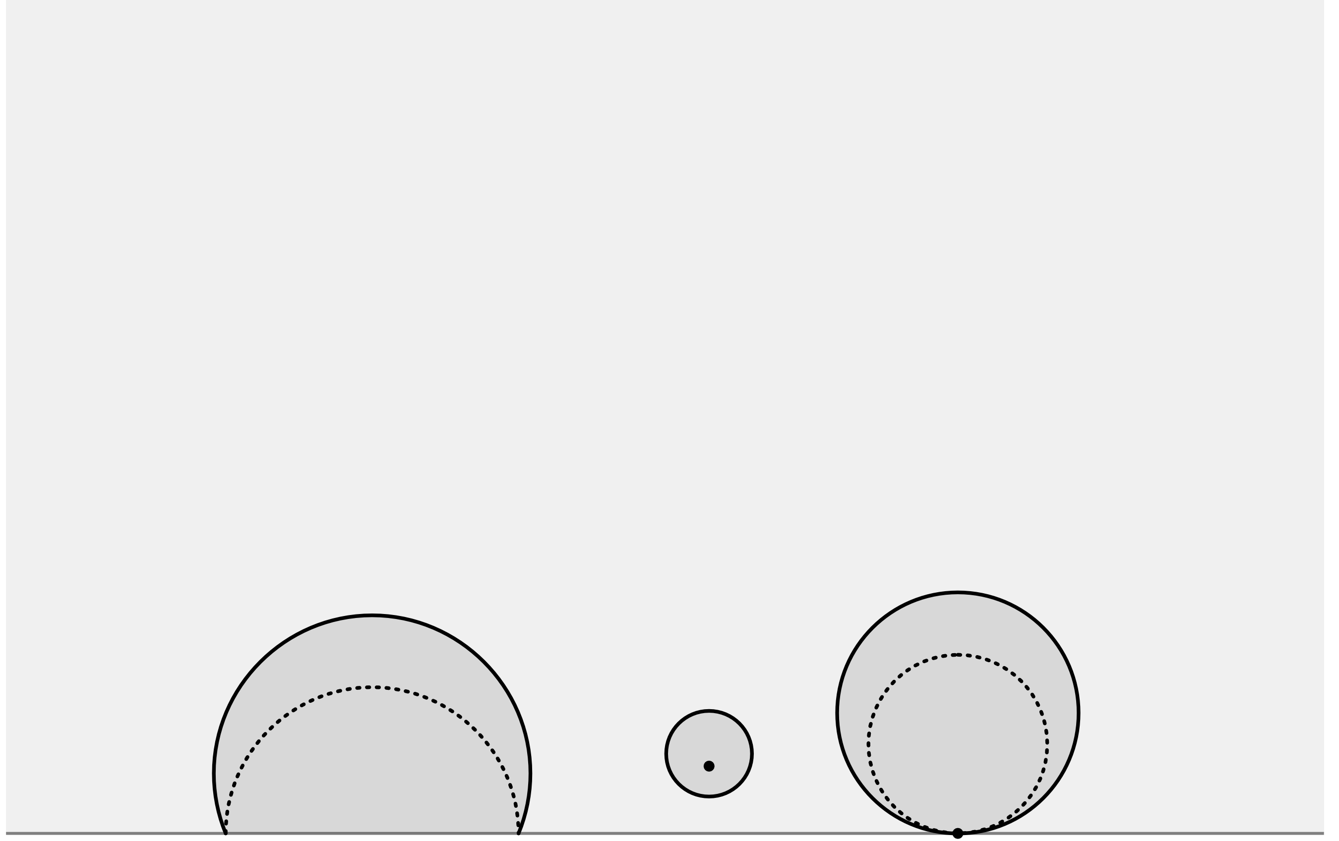
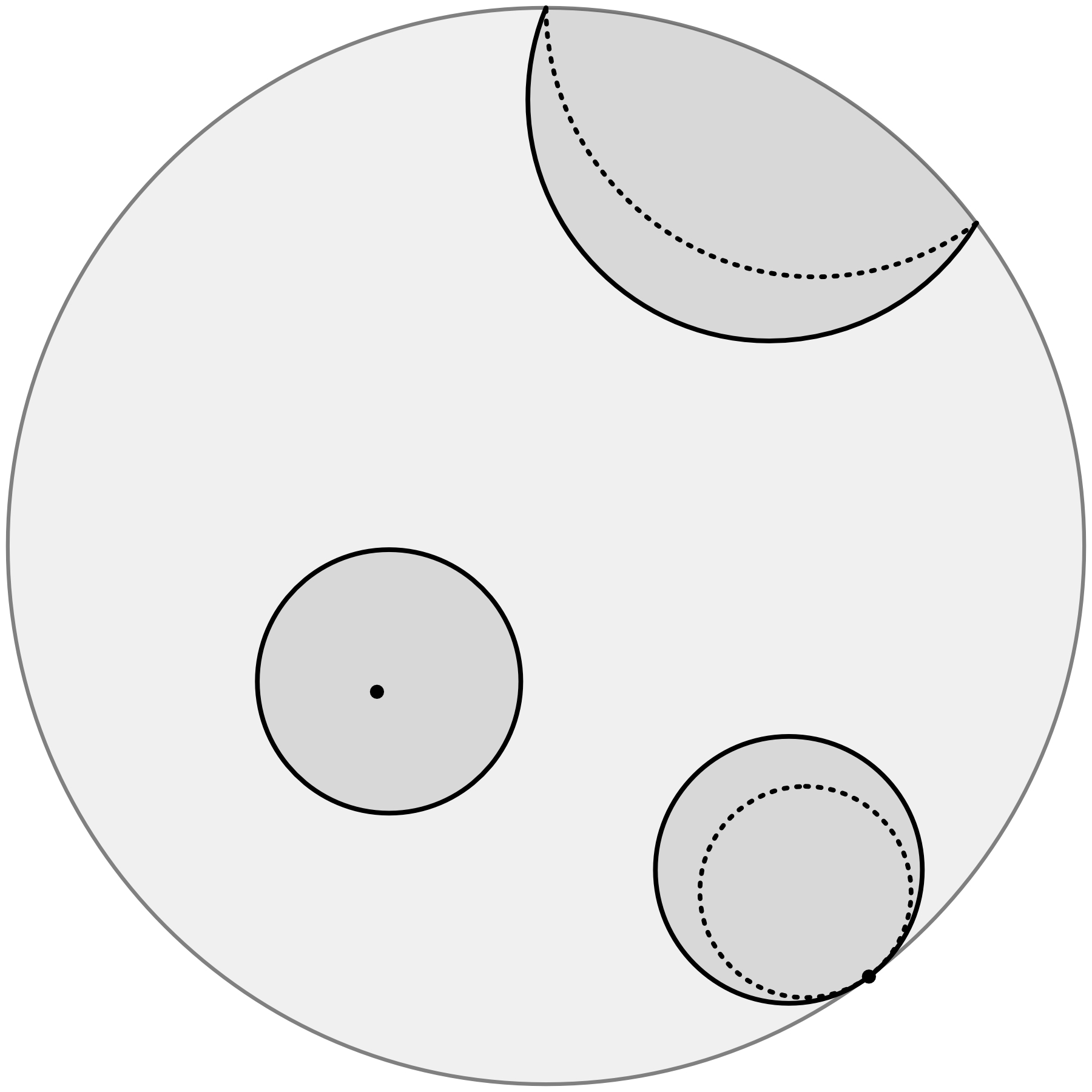
Figure 3. Left: hyperbolic cycles (solid) with their centres (dotted) and associated discs (shaded). From left to right: hypercycle, circle, horocycle. Right: using the Cayley transform $z\mapsto(z-\bm{i})/(z+\bm{i})$ we can switch to the Poincaré disc model of the hyperbolic plane.

Each hyperbolic cycle spans a pencil together with $\partial\mathbb{H}$. This pencil either contains a point in $\mathbb{H}\cup\partial\mathbb{H}$ or a hyperbolic line. These members are called the centres of the corresponding hyperbolic cycles. Furthermore, a hyperbolic cycle divides $\mathbb{H}$ into two components. For a circle or a hypercycle one of these components contains its centre and in the case of a horocycle there is a component such that the intersection of its closure in $\hat{\mathbb{C}}$ with $\partial\mathbb{H}$ is its centre. These components are called (open) circular discs, (open) horodiscs or (open) hyperdiscs, respectively. The closure of these discs will always be considered relative to $\mathbb{H}$, i.e., it is given by the union of the disc with its bounding cycle.

Lemma 2.4.

Any pencil spanned by two hyperbolic cycles, say $C_{1}$ and $C_{2}$, contains at most one hyperbolic line.

Proof.

From dimension considerations it follows that the intersection of $\{\langle X,\partial\mathbb{H}\rangle=0\}$ and $\operatorname{span}\{C_{1},C_{2}\}$ is non-empty. Furthermore, $\operatorname{span}\{C_{1},C_{2}\}\nsubset\{\langle X,\partial\mathbb{H}\rangle=0\}$ since neither $C_{1}$ nor $C_{2}$ is a hyperbolic line or a point. ∎

Definition 2.5 (radical line).

Given two hyperbolic cycles. The unique hyperbolic line, if existent, in their pencil is called their (hyperbolic) radical line.

Since we normalised $\partial\mathbb{H}$ to be the $x$-axis its complement is given by $\operatorname{Sym}(2)\subset\operatorname{Herm}(2)$. Hence, the space of hyperbolic cycles is given by $\{|X|^{2}>0\}\setminus\operatorname{Sym}(2)$ up to scaling. This can be simplified by considering an affine space parallel to $\operatorname{Sym}(2)$.

Proposition 2.6 (space of hyperbolic cycles).

The hyperbolic cycles and points of $\mathbb{H}$ can be identified with elements of $\operatorname{Sym}(2)$. In particular, the type of a cycle represented by $C\in\operatorname{Sym}(2)$ can be determined using $\langle\cdot,\cdot\rangle$ (see Figure 4):

type		norm
hypercycle		$|C|^{2}>0$
horocycle		$|C|^{2}=0$, $x_{0}>0$
circle		$0>|C|^{2}>-1$, $x_{0}>0$
point		$|C|^{2}=-1$, $x_{0}>0$.

Furthermore, two hyperbolic cycles are orthogonal iff their representatives $C_{1},C_{2}\in\operatorname{Sym}(2)$ satisfy $\langle C_{1},C_{2}\rangle=-1$.

Proof.

As described, we can identify the hyperbolic cycles with part of an affine space parallel to $\operatorname{Sym}(2)$, say $\{\langle X,\partial\mathbb{H}\rangle=1\}$. By definition, the type of a cycle $C$ is determined by the signature of $\operatorname{span}\{\partial\mathbb{H},C\}$. Our choice of affine space and Lemma 2.2 lead to the table above. Similarly, the characterisation of orthogonality follows from Lemma 2.1. ∎

Figure 4. 2D-sketch of the domains representing hyperbolic cycles: points (solid line); circles (shaded region); horocycles (dotted line); hypercycles (striped region).

2.2. Hyperbolic polygons and decorations

To a finite collection of hyperbolic circles we can naturally associate a hyperbolic polygon by considering the convex hull of their centres. We are now going to investigate how this construction can be extended to more general collections of hyperbolic cycles.

Definition 2.7 (hyperbolic polygons).

Consider a finite collection $\{C_{n}\}_{n=1}^{N}$, $N\geq 3$, of hyperbolic cycles. Suppose that their associated discs are pairwise disjoint. Their associated hyperbolic polygon is

$$\operatorname{poly}\big{(}\{C_{n}\}_{n=1}^{N}\big{)}\;\coloneq\;\left\{p\in\mathbb{H}\,:\,p=\sum_{n=1}^{N}\alpha_{n}C_{n},\;\,\alpha_{1},\dotsc,\alpha_{N}\geq 0\right\}.$$

A (convex) hyperbolic polygon (see Figure 5, left) is a subset $P\subset\mathbb{H}$ such that there is some sequence $\{C_{n}\}_{n=1}^{N}$ of hyperbolic cycles with $P=\operatorname{poly}\big{(}\{C_{n}\}_{n=1}^{N}\big{)}$.

We call a collection of hyperbolic cycles minimal if there is no $n$ such that the centre of $C_{n}$ is contained in $\operatorname{poly}\big{(}\{C_{n}\}_{n=1}^{N}\big{)}\eqcolon P$. In this case we also call $P$ a hyperbolic $N$-gon and the centres of the $C_{n}$ the vertices of $P$. In particular, $P$ is a hyperbolic triangle or quadrilateral if $N=3$ or $N=4$, respectively. By our assumption about the associated discs, we can reorder a minimal sequence of cycles defining $P$ such that there are $L_{n}\in\operatorname{Sym}(2)$ with $|L_{n}|^{2}=1$,

$$\operatorname{poly}\big{(}\{C_{n}\}_{n=1}^{N}\big{)}\;=\;\mathbb{H}\,\cap\,\bigcap_{n=1}^{N}\{\langle X,L_{n}\rangle\leq 0\}$$

and $\langle C_{n},L_{n}\rangle=0=\langle C_{n+1},L_{n}\rangle$, where $C_{N+1}=C_{1}$. The intersection $P\cap\{\langle X,L_{n}\rangle=0\}$ is a hyperbolic line segment and we call it an edge of $P$. Suppose that there are $0<M\leq N$ vertices of $P$ which are hyperbolic lines. For each such vertex there is $c_{m}\in\operatorname{Sym}(2)$ representing the centre of $C_{n_{m}}$ with $|c_{m}|^{2}=1$ and $\langle c_{m},C_{n}\rangle<0$ for all $n\neq n_{m}$. The truncation of $P$ is defined as

$$\operatorname{trunc}(P)\;\coloneq\;P\,\cap\,\bigcap_{m=1}^{M}\{\langle X,c_{m}\rangle\leq 0\}.$$

Definition 2.8 (decorated hyperbolic polygon).

Let $P$ be a hyperbolic $N$-gon and denote by $v_{1},\dotsc,v_{N}$ its vertices. A decoration of $P$ is a choice of hyperbolic cycles $C_{v_{1}},\dotsc,C_{v_{N}}$ such that $C_{v_{n}}$ is centred at $v_{n}$ and all cycles intersect the interior of the truncation of $P$. The polygon $P$ together with the cycles $C_{v_{n}}$ is called a decorated hyperbolic polygon (see Figure 5, right).

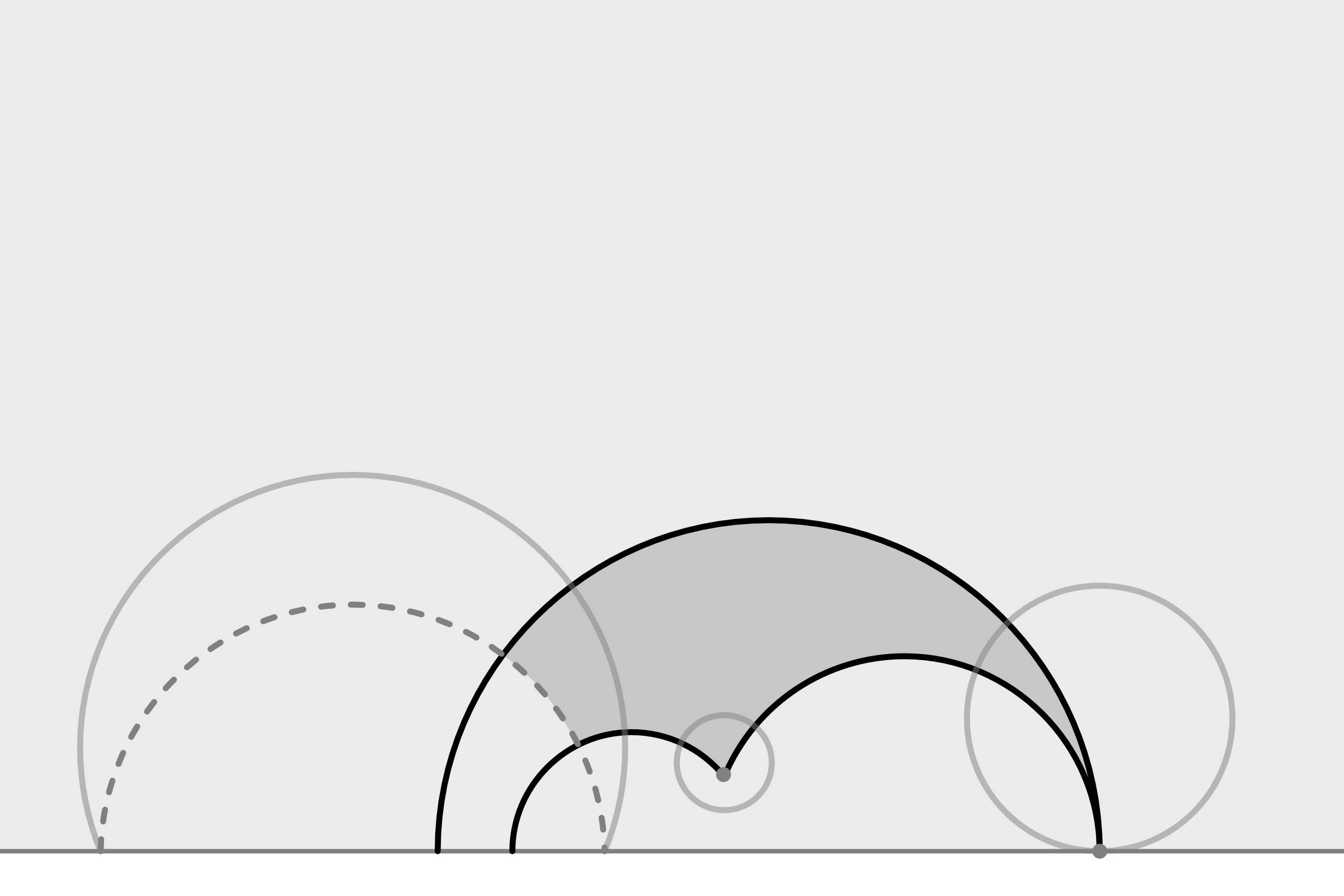
Figure 5. Left: in the Beltrami-Klein model of the hyperbolic plane a hyperbolic polygon is given by the intersection of the Euclidean unit disc with a Euclidean polygon. Vertices outside the disc correspond to hyperbolic lines by polarity (dashed lines). Right: a decorated hyperbolic triangle in the half-plane model. The truncation of the triangle is shaded.

Consider a vertex $v$ of a decorated hyperbolic polygon $P$ incident to the hyperbolic lines $L_{n}$ and $L_{m}$ with decorating cycle $C_{v}$. The (generalised) angle $\theta_{v}$ at $v$ in $P$ is defined as follows: if $v\in\mathbb{H}$ then $\theta_{v}$ is the interior angle between $L_{n}$ and $L_{m}$ in $P$. For $v\in\partial\mathbb{H}$ the angle is the hyperbolic length of the horocyclic arc $C_{v}\cap P$. Finally, if $v$ is a hyperbolic line we define $\theta_{v}$ to be the hyperbolic distance between $L_{n}$ and $L_{m}$.

For $v\notin\partial\mathbb{H}$ we define the radius $r_{v}$ of $C_{v}$ to be its distance to its centre $v$. If $v\in\partial\mathbb{H}$ we choose some horocycle $H_{v}$ centred at $v$. We call it an auxiliary centre of $C_{v}$ and the oriented hyperbolic distance $r_{v}$ between $H_{v}$ and $C_{v}$ the (auxiliary) radius of $C_{v}$. The orientation is chosen such that $r_{v}$ is negative if $C_{v}$ is contained in the horodisc bounded by $H_{v}$. Whenever it is clear from the context that we are talking about $H_{v}$ and not $v$ we might call $H_{v}$ a centre, too. Furthermore, let $e$ be an edge of $P$ contained in the line $L$ with adjacent vertices $u$ and $v$. Its (generalised) edge-length $\ell_{e}$ is the oriented distance between the (auxiliary) centres at $u$ and $v$. Clearly, the notions of auxiliary radius and edge-length depend on the choice of auxiliary centres. But we will see in the following (Lemma 2.10) that different choice, say $H_{v}$ and $\tilde{H}_{v}$, only result in a constant offset, i.e., the oriented distance between $H_{v}$ and $\tilde{H}_{v}$ (see Figure 6).

Figure 6. Definition of radius and edge-length for horocycles. Left: Concentric horocycles (solid) with auxiliary centre $H_{v}$ (dashed). The disc belonging to $H_{v}$ is shaded. Right: Edge-length between horocycles and a hyperbolic line.

We aim to relate the metric properties of decorated triangles to the representation of their cycles in $\operatorname{Sym}(2)$. Therefore, we need to introduce some extra notation. The type $\epsilon_{v}$ of a vertex $v$ is $-1$, $0$ or $+1$ depending on whether $v\in\mathbb{H}$, $v\in\partial\mathbb{H}$ or is a hyperbolic line. Furthermore, we define the angle-modifiers $\rho_{\epsilon}\colon\mathbb{R}\to\mathbb{R}$ by

$$\rho_{-1}(\theta)\coloneq\sin(\theta),\qquad\rho_{0}(\theta)\coloneq\theta,\qquad\rho_{1}(\theta)\coloneq\sinh(\theta)$$

and the length-modifiers $\tau_{\epsilon}\colon\mathbb{R}\to\mathbb{R}$ are given by

(6) $$\tau_{-1}(\ell)\coloneq\cosh(\ell),\qquad\tau_{0}(\ell)\coloneq\frac{1}{2}\mathrm{e}^{\ell},\qquad\tau_{1}(\ell)\coloneq\sinh(\ell).$$

Lemma 2.9.

Consider a hyperbolic cycle $C$ with centre of type $\epsilon=\pm 1$ and radius $r$. Then its representative in $C\in\operatorname{Sym}(2)$ satisfies

(7) $$|C|^{2}\,=\,\frac{\epsilon}{\tau_{\epsilon}^{2}(r)}.$$

Proof.

Using a Möbius transformation we can assume that the centre of the cycle is $\bm{i}$ or intersects the $y$-axis orthogonally in $\bm{i}$, respectively. The hyperbolic distance in the Poincaré metric for two points $p\bm{i},q\bm{i}\in\mathbb{H}$ on the $y$-axis takes the form

(8) $$\operatorname{dist}_{\mathbb{H}}(p\bm{i},q\bm{i})=|\ln(p)-\ln(q)|.$$

Hence, it follows that the cycle can be represented in $\operatorname{Herm}(2)$ by

(9) $$\begin{pmatrix}1&\bm{i}\tau_{\epsilon}(r)\\ -\bm{i}\tau_{\epsilon}(r)&-\epsilon\end{pmatrix}.$$

The assertion follows by direct computation. ∎

Lemma 2.10.

Given a decorated hyperbolic polygon. Denote by $\ell_{uv}$ the length of the edge between two adjacent vertices $u$ and $v$. Then the product of the cycles $C_{u},C_{v}\in\operatorname{Sym}(2)$ at these vertices is

(10) $$-\langle C_{u},C_{v}\rangle\,=\,\frac{\tau_{\epsilon_{u}\epsilon_{v}}^{\prime}(\ell_{uv})}{\tau_{\epsilon_{u}}(r_{v})\tau_{\epsilon_{v}}(r_{v})}.$$

Proof.

We begin by normalising the first cycle as in the previous Lemma 2.9. Note that equation (9) for the representative in $\operatorname{Herm}(2)$ remains valid for the horocycle passing through $0$ and $\bm{i}$ with auxiliary radius $r_{u}=0$. The second cycle is then given by

(11) $$\begin{cases}\begin{pmatrix}0&\bm{i}\\ -\bm{i}&-2\mathrm{e}^{\ell_{uv}}\end{pmatrix}&\text{if $\epsilon_{v}=0$ or}\\[14.22636pt] \begin{pmatrix}1&-\bm{i}\tau_{\epsilon_{v}}(r_{v})\mathrm{e}^{\ell_{uv}}\\ \bm{i}\tau_{\epsilon_{v}}(r_{v})\mathrm{e}^{\ell_{uv}}&-\epsilon_{v}\mathrm{e}^{2\ell_{uv}}\end{pmatrix}&\text{if $\epsilon_{v}\neq 0$.}\end{cases}$$

Again, the assertion follows by direct computation. ∎

Lemma 2.11 (hyperbolic cosine laws).

Consider a decorated hyperbolic triangle with vertices $u$, $v$ and $w$. Denote by $\ell_{uv}$, $\ell_{vw}$ and $\ell_{wu}$ the edge-lengths and suppose that $\epsilon_{v}=-1$. Then the angle $\theta_{v}$ is related to the edge-lengths by

(12) $$\cos(\theta_{v})\;=\;\frac{-\tau_{\epsilon_{w}\epsilon_{u}}^{\prime}(\ell_{wu})\,+\,\tau_{\epsilon_{u}}(\ell_{uv})\tau_{\epsilon_{w}}(\ell_{vw})}{\tau_{\epsilon_{u}}^{\prime}(\ell_{uv})\tau_{\epsilon_{w}}^{\prime}(\ell_{vw})}.$$

Proof.

These relations follow either by direct computation for the different cases [Ratcliffe94]*§3.5 or using a combined approach by analysing bases in $\operatorname{Sym}(2)$ [Thurston97]*Section 2.4. ∎

Definition 2.12 (modified tangent distance).

Let $C$ be hyperbolic cycle of type $\epsilon$ with (auxiliary) centre $c$ and radius $r$. The modified tangent distance between $C$ and a point $x\in\mathbb{H}$ is

$$\operatorname{td}_{x}(c,r)\,\coloneq\,\operatorname{td}_{x}(C)\,\coloneq\,\frac{\tau_{\epsilon}(\operatorname{dist}_{\mathbb{H}}(c,x))}{\tau_{\epsilon}(r)}.$$

Here, we orient $\operatorname{dist}_{\mathbb{H}}$ such that $\operatorname{dist}_{\mathbb{H}}(c,x)>0$ iff $\langle C,x\rangle<(\epsilon-1)/\tau_{\epsilon}(r)$ (compare to Lemma 2.10). Note that this condition is satisfied for all points $x\neq c$ if $\epsilon=-1$.

Lemma 2.13.

Let $C_{1}$ and $C_{2}$ be hyperbolic cycles whose associated discs do not contain each other, respectively. Then the radical line of $C_{1}$ and $C_{2}$ exists and is given by $\{x\in\mathbb{H}:\operatorname{td}_{x}(C_{1})=\operatorname{td}_{x}(C_{2})\}$.

Proof.

Suppose a point $x\in\mathbb{H}$ is not contained in the disc associated to $C_{n}$, $n=1,2$. By Lemma 2.11, $\operatorname{td}_{x}(C_{n})=\cosh(\delta)$ where $\delta$ is the hyperbolic length of the hyperbolic segments which starts in $x$ and ends at a tangent point with $C_{n}$ (see Figure 7). Thus, if there is a point $x$ such that

(13) $$\operatorname{td}_{x}(C_{1})\,=\,\operatorname{td}_{x}(C_{2})$$

then $x$ is the centre of a hyperbolic circle $C$ which is orthogonal to both $C_{1}$ and $C_{2}$.

Figure 7. The modified tangent distance between a cycle $C$ and a point $x$ outside its associated disc is the hyperbolic cosine of the length of the tangential segment to $C$ starting at $x$. It can be computed using right-angled hyperbolic triangles.

Now, consider the function $f\colon x\mapsto\operatorname{td}_{x}(C_{1})-\operatorname{td}_{x}(C_{2})$. It is continuous. Furthermore, we find $x_{+},x_{-}\in\mathbb{H}$ with $f(x_{+})>0$ and $f(x_{-})<0$ because of our assumption about the associated discs. It follows, considering two non-intersecting continuous path starting at $x_{+}$ and ending at $x_{-}$, that there are $p,\tilde{p}\in\mathbb{H}$ which satisfy equation (13). We already observed that they are the centres of two hyperbolic circles which are orthogonal to both $C_{1}$ and $C_{2}$. Hence, they span the dual pencil of $C_{1}$ and $C_{2}$. We conclude that the hyperbolic line connecting $p$ and $\tilde{p}$ is in the pencil spanned by $C_{1}$ and $C_{2}$, that is, the unique radical line of $C_{1}$ and $C_{2}$ (Lemma 2.4). ∎

Corollary 2.14.

Let $C_{1}$ be a hyperbolic cycle with (auxiliary) centre $c_{1}$ and $C_{2}$ a circle with centre $c_{2}$. In addition to the assumptions of Lemma 2.13 we require that $\operatorname{dist}_{\mathbb{H}}(c_{1},c_{2})>0$. The orientation is chosen as in Definition 2.12. Then the radical line of $C_{1}$ and $C_{2}$ intersects the hyperbolic ray starting at $c_{2}$ extending towards the centre of $C_{1}$ iff $\tau_{\epsilon_{1}}(r_{1})/\cosh(r_{2})<\tau_{\epsilon_{1}}(\operatorname{dist}_{\mathbb{H}}(c_{1},c_{2}))$.

Suppose $C_{1},C_{2},C_{3}\in\operatorname{Sym}(2)$ are the vertex cycles of a decorated hyperbolic triangle. They form a basis of $\operatorname{Sym}(2)$. Hence, they determine a unique affine plane in $\operatorname{Sym}(2)$. There is a unique $F\in\operatorname{Sym}(2)$ such that this plane is given by $\{\langle X,F\rangle=-1\}$. We call $F$ the face-vector of the triangle.

Lemma 2.15.

The three radical lines defined by a decorated hyperbolic triangle whose vertex discs do not contain each other, respectively, either intersect in a common point in $\mathbb{H}\cup\partial\mathbb{H}$ or are all orthogonal to a common hyperbolic line.

Proof.

Let $C_{1}$, $C_{2}$ and $C_{3}$ denote the vertex cycles and $F$ their face-vector. From Lemma 2.10 and Lemma 2.13 we deduce that the radical line of the vertex cycles $C_{m}$ and $C_{n}$, $m\neq n$, is given by $\{\langle X,C_{n}-C_{m}\rangle=0\}$. Since $\langle F,C_{n}\rangle=-1$, $n=1,2,3$, we see that

$$\bigcap_{n\neq m}\{\langle X,C_{n}-C_{m}\rangle=0\}\,=\,\operatorname{span}\{F\}.\qed$$

By definition the vertices of an associated hyperbolic polygon are centres of the defining cycles. But in general not all centres need to be vertices, too. We are now going to find some sufficient conditions in terms of the intersection angles the cycles. It is understood to be the interior intersection angle of their associated discs.

Lemma 2.16.

Consider two vertex cycles, say $C_{1}$ and $C_{2}$. Their associated discs either do not intersect or intersect at most with an angle of $\pi/2$ if $\langle C_{1},C_{2}\rangle\leq-1$.

Proof.

This assertion follows from combining Lemma 2.11 and Lemma 2.10. ∎

Lemma 2.17.

Consider a decorated hyperbolic triangle with vertex cycles given by $C_{1},C_{2},C_{3}\in\operatorname{Sym}(2)$. Let $F$ be their face-vector. Suppose that $X=\alpha_{1}C_{1}+\alpha_{2}C_{2}+\alpha_{3}C_{3}$ is a hyperbolic cycle with $\alpha_{1},\alpha_{2},\alpha_{3}\geq 0$ and $\langle F,X\rangle\leq-1$. Then there is an $n$ such that $\langle C_{n},X\rangle>-1$.

Proof.

From $\langle F,C_{i}\rangle=-1$, we deduce that

$$-1\,\geq\,\langle F,X\rangle\,=\,-(\alpha_{1}+\alpha_{2}+\alpha_{3}).$$

By assumption $X$ is a hyperbolic cycle. Proposition 2.6 leads to

(14) $$|X|^{2}\,=\,\alpha_{1}\langle C_{1},X\rangle\,+\,\alpha_{2}\langle C_{2},X\rangle\,+\,\alpha_{3}\langle C_{3},X\rangle\,>\,-1.$$

Combining these two inequalities yields the result. ∎

Proposition 2.18.

Let $C_{1},\dotsc,C_{N}$ be hyperbolic cycles with pairwise non-intersecting discs. Suppose that there is $F\in\operatorname{Sym}(2)$ such that $\langle F,C_{n}\rangle=-1$ for all $n=1,\dotsc,N$. Then the centre of each $C_{n}$ is a vertex of the associated hyperbolic polygon $\operatorname{poly}(C_{1},\dotsc,C_{N})$.

Proof.

Suppose otherwise. Then there are four cycles, w.l.o.g., $C_{1}$, $C_{2}$, $C_{3}$ and $C_{4}$, such that $C_{4}=\alpha_{1}C_{1}+\alpha_{2}C_{2}+\alpha_{3}C_{3}$ with $\alpha_{1},\alpha_{2},\alpha_{3}\geq 0$. By Lemma 2.17 there is an $n\in\{1,2,3\}$ such that $\langle C_{4},C_{n}\rangle>-1$. Hence, Lemma 2.16 implies that the discs of $C_{4}$ and $C_{n}$ intersect. This contradicts our assumption. ∎

2.3. The local Delaunay condition

A triangulated decorated hyperbolic quadrilateral is the union of two decorated hyperbolic triangles with disjoint interiors which share an edge and the corresponding vertex cycles. For the rest of the section we refer to them simply as decorated quadrilaterals. The two triangles give a triangulation of the quadrilateral and their common edge is called diagonal. Combinatorially there are two triangulation for each quadrilateral. This change of combinatorics is called an edge-flip. The diagonal of a decorated quadrilateral is called flippable if its edge-flip can be geometrically realised in $\mathbb{H}$. It is immediate that a diagonal is flippable iff the decorated quadrilateral is strictly convex. Note that a decorated quadrilateral in the sense of this section need not be convex. Hence it is not necessarily a decorated hyperbolic $4$-gon as defined in Definition 2.8. Still, a decorated quadrilateral is always strictly convex if it has no vertices contained in $\mathbb{H}$.

Definition 2.19 (local Delaunay condition).

Consider a decorated quadrilateral with vertex cycles $C_{1},C_{2},C_{3},C_{4}\in\operatorname{Sym}(2)$ such that $C_{2}$ and $C_{3}$ belong to the diagonal. Denote by $F_{123},F_{234}\in\operatorname{Sym}(2)$ the face-vectors. We say that the diagonal satisfies the local Delaunay condition, or is local Delaunay, iff

(15) $$\langle C_{1},F_{234}\rangle\,\leq\,-1\qquad\text{and}\qquad\langle C_{4},F_{123}\rangle\,\leq\,-1.$$

Remark 2.1.

Suppose that $|F_{123}|^{2}>-1$. Then it represents a hyperbolic cycle which is orthogonal to $C_{1}$, $C_{2}$ and $C_{3}$. The proof of Lemma 2.15 shows that the centre of $F_{123}$ is the “intersection point” of the radical lines of the triangle corresponding to $F_{123}$. In addition, Lemma 2.16 shows that the local Delaunay is equivalent to $F_{123}$ intersecting $C_{4}$ at most orthogonally.

In the following we are going to derive a way to determine the local Delaunay condition just by intrinsic properties of the decorated quadrilateral. To this end, again denote by $C_{1}$, $C_{2}$ and $C_{3}$ the vertex cycles of a decorated hyperbolic triangle. For any permutation $(m,n,k)$ of $\{1,2,3\}$ the subspace spanned by $C_{m}$ and $C_{n}$ corresponds to an edge of the triangle. Therefore, there is a $L_{k}\in\operatorname{Sym}(2)$ with $|L_{k}|^{2}=1$ such that this subspace is given by the complement of $L_{k}$ in $\operatorname{Sym}(2)$. The $L_{k}$ can be chosen in such a way that $\langle L_{k},C_{k}\rangle<0$. Denote by $r_{n}$ the radius and by $\epsilon_{n}$ the type of the cycle represented by $C_{n}$. Furthermore, let $\theta_{n}$ be the interior angle at the vertex $n$ and $d_{n}$ be the (oriented) distance between the (auxiliary) centre of $C_{n}$ and the line $L_{n}$ (see Figure 8). Note that the $d_{n}$ can be computed from the edge-lengths.

Figure 8. Notation in a decorated hyperbolic triangle.

Lemma 2.20.

The $L_{k}$ form a basis of $\operatorname{Sym}(2)$. Their dual basis is $-\tau_{\epsilon_{k}}(r_{k})/\tau_{\epsilon_{k}}^{\prime}(d_{k})\,C_{k}$.

Proof.

By construction $\langle L_{k},C_{m}\rangle=0=\langle L_{k},C_{m}\rangle$. Hence, up to a scalar, $C_{k}$ is the dual vector of $L_{k}$. The scale factor follows from Lemma 2.10. ∎

Lemma 2.21.

Let $L_{1},L_{2}\in\operatorname{Herm}(2)$ be representatives of two hyperbolic lines. Suppose that $|L_{n}|^{2}=1$. Denote by $\theta$ the generalised angle between $L_{1}$ and $L_{2}$ and by $\epsilon$ the type of there common vertex. Then

(16) $$|\rho_{\epsilon}^{\prime}(\theta)|\,=\,|\langle L_{1},L_{2}\rangle|.$$

Proof.

We can normalise the first line to be the $y$-axis. Then its representative is given by $L_{1}=\left(\begin{smallmatrix}0&1\\ 1&0\end{smallmatrix}\right)$. The representative of the second line can now be obtained by applying the appropriate hyperbolic motion to $L_{1}$, i.e.,

(17) $$\begin{pmatrix}\sin(\theta)&1-\cos(\theta)\\ \cos(\theta)-1&\sin(\theta)\end{pmatrix},\qquad\begin{pmatrix}1&0\\ \theta&1\end{pmatrix}\qquad\text{or}\qquad\begin{pmatrix}\sinh(\theta)&1-\cosh(\theta)\\ 1-\cosh(\theta)&\sinh(\theta)\end{pmatrix}$$

depending on whether the common vertex of $L_{1}$ and $L_{2}$ has type $-1$, $0$ or $1$, respectively. The rest of the proof follows by direct computation. ∎

Lemma 2.22.

Consider a decorated hyperbolic triangle with face-vector $F$. Define $t_{n}\coloneq\langle F,L_{n}\rangle$. The $t_{n}$ can be computed by

(18) $$\begin{pmatrix}t_{1}\\ t_{2}\\ t_{3}\end{pmatrix}\,=\,\begin{pmatrix}1&-\rho_{\epsilon_{3}}^{\prime}(\theta_{3})&-\rho_{\epsilon_{2}}^{\prime}(\theta_{2})\\ -\rho_{\epsilon_{3}}^{\prime}(\theta_{3})&1&-\rho_{\epsilon_{1}}^{\prime}(\theta_{1})\\ -\rho_{\epsilon_{2}}^{\prime}(\theta_{2})&-\rho_{\epsilon_{1}}^{\prime}(\theta_{1})&1\end{pmatrix}\begin{pmatrix}\tau_{\epsilon_{1}}(r_{1})/\tau_{\epsilon_{1}}^{\prime}(d_{1})\\ \tau_{\epsilon_{2}}(r_{2})/\tau_{\epsilon_{2}}^{\prime}(d_{2})\\ \tau_{\epsilon_{3}}(r_{3})/\tau_{\epsilon_{3}}^{\prime}(d_{3})\end{pmatrix}.$$

Proof.

Using the defining property of the face-vector and Lemma 2.20 we see

(19) $$F\,=\,\sum_{n=1}^{3}\langle-\frac{\tau_{\epsilon_{n}}(r_{n})}{\tau_{\epsilon_{n}}^{\prime}(d_{n})}C_{n},F\rangle\,L_{n}\,=\,\sum_{n=1}^{3}\frac{\tau_{\epsilon_{n}}(r_{n})}{\tau_{\epsilon_{n}}^{\prime}(d_{n})}\,L_{n}.$$

The result follows from Lemma 2.21. Note that the sign of the generalised angles follows from our choice of $L_{n}$. ∎

Definition 2.23 (tilts of a decorated hyperbolic triangle).

The $t_{n}$ in the Lemma 2.22 above is called the tilt of the decorated hyperbolic triangle along the edge $L_{n}$.

Remark 2.2.

The tilts have a special geometric meaning if $|F|^{2}>-1$. In this case $F$ represents the unique hyperbolic cycle orthogonal to all vertex-cycles of the decorated triangle. Thus, by Lemma 2.10, the tilt $t_{n}$ is given by the (oriented) distance of the centre of $F$ to $L_{n}$ divided by the radius of $F$. By Remark 2.1, this distance is measured along the radical line belonging to the edge $L_{n}$.

Proposition 2.24 (local Delaunay condition).

Given a decorated quadrilateral. Let $t_{\mathrm{left}}$ and $t_{\mathrm{right}}$ be the tilts along its diagonal relative to the two triangles constituting the quadrilateral. Then the interior edge is locally Delaunay iff its tilts satisfy

(20) $$t_{\mathrm{left}}\,+\,t_{\mathrm{right}}\,\leq\,0.$$

Proof.

This proof follows the ideas in [Ushijima02]. Let $C_{1},\dotsc,C_{4}\in\operatorname{Sym}(2)$ denote the vertex cycles of the decorated quadrilateral such that $C_{1}$, $C_{2}$ and $C_{3}$ belong to the left and $C_{2}$, $C_{3}$ and $C_{4}$ to the right triangle. Since the subspace spanned by $C_{2}$ and $C_{3}$ corresponds to the common edge of the triangles there is an $L\in\operatorname{Sym}(2)$ with $|L|^{2}=1$ and $\langle L,C_{2}\rangle=0=\langle L,C_{3}\rangle$. We can normalise $L$ such that $\langle L,C_{1}\rangle<0$ and $\langle L,C_{4}\rangle>0$. It follows that $\{L,C_{2},C_{3}\}$ is a basis of $\operatorname{Sym}(2)$. Using this basis we can represent the remaining vertex cycles as linear combinations:

(21) $$C_{1}\,=\,\alpha L\,+\,\alpha_{2}C_{2}\,+\,\alpha_{3}C_{3}\qquad\text{and}\qquad C_{4}\,=\,\tilde{\alpha}L\,+\,\tilde{\alpha}_{2}C_{2}\,+\,\tilde{\alpha}_{3}C_{3}.$$

Note that $\tilde{\alpha}>0$ by our choice of $L$. Furthermore, we get the representation

(22) $$F_{\mathrm{left}}\,=\,\beta L\,+\,\beta_{2}C_{2}\,+\,\beta_{3}C_{3}\qquad\text{and}\qquad F_{\mathrm{right}}\,=\,\tilde{\beta}L\,+\,\tilde{\beta}_{2}C_{2}\,+\,\tilde{\beta}_{3}C_{3}$$

for the face-vectors $F_{\mathrm{left}}$ and $F_{\mathrm{right}}$ of the left and right triangle, respectively. By the defining property of the face-vectors we see that $-1=\langle C_{i},F_{\mathrm{right}}\rangle=\tilde{\beta_{2}}\langle C_{i},C_{2}\rangle+\tilde{\beta_{3}}\langle C_{i},C_{3}\rangle$ for $i=2,3$. A similar equation holds for $\langle C_{i},F_{\mathrm{left}}\rangle$. Hence, we compute

(23) $$-1 \,=\,\langle C_{4},F_{\mathrm{right}}\rangle$$

(24) $$\,=\,\tilde{\alpha}\tilde{\beta}\,+\,\tilde{\alpha}_{2}(\tilde{\beta}_{2}\langle C_{2},C_{2}\rangle+\tilde{\beta}_{3}\langle C_{2},C_{3}\rangle)\,+\,\tilde{\alpha}_{3}(\tilde{\beta}_{2}\langle C_{3},C_{2}\rangle+\tilde{\beta}_{3}\langle C_{3},C_{3}\rangle)$$

(25) $$\,=\,\tilde{\alpha}\tilde{\beta}\,-\,\tilde{\alpha}_{2}\,-\,\tilde{\alpha}_{3}.$$

Finally, we see that the local Delaunay condition (15) is given by

(26) $$-1\,\geq\,\langle C_{4},F_{\mathrm{left}}\rangle\,=\,\tilde{\alpha}\beta\,-\,\tilde{\alpha}_{2}\,-\,\tilde{\alpha}_{3}\,=\,\tilde{\alpha}(\beta-\tilde{\beta})\,-\,1.$$

Observing that $\beta=t_{\mathrm{left}}$ and $\tilde{\beta}=-t_{\mathrm{right}}$ yields the claim. ∎

Example 2.25.

Consider a decorated quadrilateral by gluing two copies of an isosceles decorated triangle along one of their legs, respectively. Note that by construction the vertex cycles at the base are of the same type and radius. Suppose that the radii satisfy the condition given in Corollary 2.14. By symmetry, the radical line of the cycles at the base and the altitude erected over the base of the isosceles triangle coincide. Hence, the tilt with respect to one leg, and thus both, is negative (see Remark 2.2 and Figure 9, left). It follows that the diagonal satisfies the local Delaunay condition.

Figure 9. Left: an isosceles hyperbolic triangle. The centre of the hyperbolic cycle which is orthogonal to all vertex cycles lies always to the left of the legs of the triangle. Right: a concave decorated quadrilateral with radical lines (dashed). Corollary 2.14 provides conditions for the radical lines to intersect the interior of the edges. This guarantees that the diagonal satisfies the local Delaunay condition.

Proposition 2.26.

Suppose a quadrilateral is decorated such that the radii satisfy the condition given in Corollary 2.14. Then it can always be triangulated such that its diagonal satisfies the local Delaunay condition. Equivalently, if the diagonal is not local Delaunay then it is flippable and the new diagonal is local Delaunay.

Proof.

The vertex cycles give rise to an affine tetrahedron in $\operatorname{Sym}(2)$. A triangulation of the decorated quadrilateral whose diagonal is local Delaunay corresponds to the lower convex hull of this tetrahedron. If the decorated quadrilateral is strictly convex then the lower and upper convex hulls project to the two possible triangulations of the quadrilateral. Hence one of them is locally Delaunay.

Should the quadrilateral be not strictly convex then it possesses only one (geometric) triangulation. Let $C_{1},\dotsc,C_{4}\in\operatorname{Sym}(2)$ denote the vertex cycles of the decorated quadrilateral as indicated in Figure 9, right. The dual pencil to the pencil spanned by $C_{2}$ and $C_{3}$ is given by $F_{\lambda}\coloneq F_{0}\,+\,\lambda\,L_{23},$ where $L_{23}$ is the line supporting the diagonal such that $\langle L_{23},C_{1}\rangle<0$ and $F_{0}\in\operatorname{Sym}(2)$ satisfies $\langle C_{2},F_{0}\rangle=\langle C_{3},F_{0}\rangle=\langle L_{23},F_{0}\rangle=0$. There are $\lambda_{n}$, $n\in\{1,4\}$, such that $F_{\lambda_{n}}$ is the face-vector of the left or right triangle, respectively. Equivalently, $\langle C_{n},F_{\lambda_{n}}\rangle=-1$. It follows that $\langle C_{1},F_{\lambda}\rangle<-1$ for all $\lambda>\lambda_{1}$. Corollary 2.14 grants that the radical lines intersect their corresponding edges. Furthermore, the diagonal of the triangulation is incident to a vertex of type $-1$ which has an interior angle sum $\geq\pi$. Thus, using Lemma 2.14, we deduce $\lambda_{2}>\lambda_{1}$. ∎

3. Decorated surfaces and their tessellations

3.1. Decorated hyperbolic surfaces of finite type

Let $\bar{\Sigma}$ be a closed orientable surface, that is, a closed orientable $2$-manifold, and $V\subset\bar{\Sigma}$ a finite set of points partitioned into $V_{-1}\cup V_{0}\cup V_{1}=V$. This partition determines a type $\epsilon_{v}\in\{-1,0,1\}$ for each point $v\in V$. Note that it is allowed for some $V_{\epsilon}$ to be empty. A complete path metric $\operatorname{dist}_{\Sigma}$ on $\Sigma\coloneq\bar{\Sigma}\setminus(V_{0}\cup V_{1})$ is hyperbolic if there is a cell-complex homeomorphic to $\bar{\Sigma}$ with $0$-cells given by $V$ such that each open $2$-cell endowed with the restriction of $\operatorname{dist}_{\Sigma}$ is isometric to a hyperbolic polygon whose vertices have the same type as the corresponding points in $V$. For more information on path metrics we refer the reader to [BridsonHaefliger99, CooperEtAl00]. We call $\Sigma$ together with $\operatorname{dist}_{\Sigma}$ a hyperbolic surface of finite type, or short hyperbolic surface. The restriction $\operatorname{trunc}(\Sigma)\subseteq\Sigma$ such that each restricted $2$-cell is isometric to the corresponding truncated hyperbolic polygon is the truncation of $\Sigma$.

The $1$-cells of the cell-complex above straighten to geodesics in $\Sigma$. Therefore, we call it a geodesic tessellation of $\Sigma$. In general there are infinitely many geodesic tessellations for a given hyperbolic surface. If each $2$-cell is isometric to a hyperbolic triangle we call the tessellation a triangulation. We also refer to the $0$-cells as vertices, the $1$-cells as edges and the $2$-cells as faces. Finally, a decoration of a hyperbolic surface is a choice of decoration for each face such that it is consistent along the common edges of each pair of neighbouring faces (more details are given in section 4). Note that a decoration is independent of the tessellation since it can be completely described by the path metric $\operatorname{dist}_{\Sigma}$.

Example 3.1.

Let $\Gamma<\operatorname{PSL}(2;\mathbb{R})$ be a finitely generated non-elementary Fuchsian group, i.e., it has a finite-sided fundamental domain (see [Beardon83]*§10.1). The quotient $\Sigma\coloneq\mathbb{H}/\Gamma$ is a hyperbolic surface of finite type (see Figure 1). A triangulation of $\Sigma$ can be obtained by triangulating the fundamental domain with hyperbolic triangles. Using the Beltrami-Klein model this is just triangulating a finite-sided convex polygon in the Euclidean sense. Identifying the sides of this Euclidean polygon according to the action of $\Gamma$ we obtain a closed surface homeomorphic to $\bar{\Sigma}$. If we decorate these triangles consistently with the action of $\Gamma$, i.e., identified vertices get cycles with the same radius, we obtain a decoration of $\Sigma$.

A decoration introduces about each vertex $v\in V$ of a hyperbolic surface $\Sigma$ a closed curve: the vertex cycle $C_{v}$. These are special constant curvature curves in $\Sigma$. A decorated hyperbolic surface is thus a pair $(\Sigma,\{C_{v}\}_{v\in V})$. Furthermore, the notions introduced in the local setting (section 2.2), e.g., centres, vertex discs, radius, edge-length, etc., carry over to decorated hyperbolic surfaces. In particular, we denote the disc associated with $C_{v}$ by $D_{v}$ and its radius by $r_{v}$. The weight-vector $\omega\coloneq(\tau_{\epsilon_{v}}(r_{v}))_{v\in V}$ determines the decoration. We also write $\Sigma^{\omega}$ for the hyperbolic surface $\Sigma$ decorated with $\omega$. Note that the centres of hypercycles, i.e., $v\in V_{1}$, are simple closed geodesics. In the following, if not mentioned otherwise, we assume the auxiliary centre about a vertex $v\in V_{0}$ to be chosen such that it does not intersect any other vertex cycle $C_{\tilde{v}}$. Slightly abusing notation, we write $\operatorname{dist}_{\Sigma}(x,v)$ for the distance between a point $x\in\Sigma$ and the (auxiliary) centre of the vertex cycle $C_{v}$. Similarly, $\operatorname{dist}_{\Sigma}(v,\tilde{v})$ will be the smallest non-zero distance between the centres of the vertex cycles $C_{v}$ and $C_{\tilde{v}}$.

Lemma 3.2.

Let $\Sigma^{\omega}$ be a decorated hyperbolic surface with non-intersecting vertex discs. For each pair of vertex cycles, say $C_{v_{0}}$ and $C_{v_{1}}$, and $L>0$ there is only a finite number of geodesic arcs which are orthogonal to both cycles and their length is $\leq L$.

Proof.

Denote by $\mathcal{A}$ the set of all constant speed parametrised arcs $\gamma\colon[0,L]\to\Sigma$ with $\gamma(0)\in C_{v_{0}}$ and $\gamma(1)\in C_{v_{1}}$. We endow $\mathcal{A}$ with the topology of uniform convergence induced by the path metric $\operatorname{dist}_{\Sigma}$. Furthermore, let $\mathcal{A}_{L}\subset\mathcal{A}$ be the subset of all geodesic arcs orthogonal to $C_{v_{0}}$ and $C_{v_{1}}$ with length $\leq L$.

The family $\mathcal{A}_{L}$ is equicontinuous and has bounded diameter. Indeed, $1$ is a uniform Lipschitz constant for $\mathcal{A}_{L}$. To see the boundedness of the diameter restrict $\Sigma$ as follows: for each vertex $v\in V_{0}\setminus\{v_{0},v_{1}\}$ choose a horocycle $C_{v}$ with $\operatorname{dist}_{\Sigma}(C_{v},C_{v_{0}}\cup C_{v_{1}})>L$. Then denote by $\Sigma^{\prime}\subseteq\Sigma$ the surface obtained by removing the horodiscs associated to the $C_{v}$ from the truncation $\operatorname{trunc}(\Sigma)$. The surface $\Sigma^{\prime}$ is compact and contains the support of all arcs contained in $\mathcal{A}_{L}$. Thus the diameter of $\mathcal{A}_{L}$ is at most the diameter of $\Sigma^{\prime}$.

Using the Arzelà-Ascoli theorem we conclude that $\mathcal{A}_{L}$ is compact in $\mathcal{A}$. Finally, we observe that the elements of $\mathcal{A}_{L}$ are isolated with respect to the uniform topology. Equivalently, because they are locally length minimising, each such geodesic arc possess a tubular neighbourhood which can not completely contain another element form $\mathcal{A}_{L}$. Hence, $\mathcal{A}_{L}$ has to be a finite set. ∎

3.2. Weighted Delaunay tessellations

Assume for the rest of this section 3.2 that $\Sigma^{\omega}$ is decorated with non-intersecting vertex discs. Define $\Sigma^{\prime}\coloneq\Sigma\setminus\bigcup_{v\in V}D_{v}$. By assumption, $\Sigma^{\prime}$ is a compact connected surface with $|V|$ boundary components. A properly immersed (circular) disc $(\varphi,D)$ is a continuous map $\varphi\colon\bar{D}\to\Sigma$, where $D\subset\mathbb{H}$ is a circular disc and $\bar{D}$ its closure, such that $\varphi|_{D}$ is an isometric immersion, i.e., each point in $D$ possesses a neighbourhood which is mapped isometrically, and the circle $\varphi(\partial D)$ intersects no $C_{v}$ more then orthogonally. As in the local setting (section 2.2) the intersection angle is understood to be the interior intersection angle of the associated discs.

Let $N\geq 2$ be a positive integer. Suppose there is a properly immersed disc $(\varphi,D)$ such that $\varphi^{-1}(\bigcup_{v\in V^{\prime}}\bar{D}_{v})$ consists of exactly $N$ connected components, where $v\in V^{\prime}\subseteq V$ iff $C_{v}$ intersects $\varphi(\partial D)$ orthogonally. To each of these connected components corresponds a hyperbolic cycle in $\mathbb{H}$ because $\varphi$ is isometric. We refer to them as the vertex cycles pulled back by $\varphi$. Denote them by $C_{1},\dotsc,C_{N}$. Then we call $\Sigma^{\prime}\cap\varphi(\operatorname{poly}(C_{1},\dotsc,C_{N})\cap D)$ a truncated $N$-vertex cell and $\varphi|_{\operatorname{poly}(C_{1},\dotsc,C_{N})\cap D}$ is its attachment map. Note that $\operatorname{poly}(C_{1},\dots,C_{N})$ is well defined by Proposition 2.18 and our assumption about the decoration.

Definition 3.3 (weighted Delaunay tessellation, non-intersecting vertex discs).

Let $\Sigma^{\omega}$ be a decorated hyperbolic surface with non-intersecting vertex discs. Geodesically extending the truncated vertex cells into the vertex discs defines a geodesic tessellation of $\Sigma$. It is called the weighted Delaunay tessellation of $\Sigma^{\omega}$. We refer to the extended truncated $2$-vertex cells as Delaunay $1$-cells and to the extended truncated $N$-vertex cells with $N\geq 3$ as Delaunay $2$-cells.

Remark 3.1.

The assumption about non-intersecting vertex discs is important to ensure the existence of properly immersed discs. For a surface without cone-points, i.e., $V_{-1}=\emptyset$, this poses no real loss of generality. In these cases, we can consider the rescaled weights $s\omega$, where $s$ is a small positive scalar. If $s$ is small enough, it follows that $s\omega$ induces non-intersecting vertex discs and Corollary 4.2 will guaranty that $\omega$ and $s\omega$ induce the same weighted Delaunay tessellation. We note that this observation was already utilised in the classical Epstein-Penner convex hull construction.

Theorem 3.4 (well-definedness of weighted Delaunay tessellations).

The weighted Delaunay tessellation defined in Definition 3.3 is a geodesic tessellation of $\Sigma$.

Proof.

First, we observe that the truncated $2$-vertex cells are geodesic segments since they are isometric images of hyperbolic segments in $\mathbb{H}$. Each such truncated $2$-vertex cell intersects its two vertex cycles orthogonally. Hence, we can geodesically extend the segments into the corresponding vertex discs. Lemma 3.6 shows that truncated $2$-vertex cells do not intersect, so lifted to $\bar{\Sigma}$ they form an embedded $1$-dimensional cell-complex with vertex set $V$.

Now, Lemma 3.5 grants that the interiors of truncated $N$-vertex cells, $N\geq 3$, are homeomorphic to open discs. Their boundary is mapped into the union of the vertex cycles with the truncated $2$-vertex cells. Furthermore, the truncated $2$-vertex cells do not intersect the interiors of the truncated $N$-vertex cells. Thus, the truncated $N$-vertex cells can be extended into the vertex discs along with the truncated $2$-vertex cells. All ideas needed to prove these assertions are presented in the rest of this section. We omit further details.

Finally, by Lemma 3.7, we see that every point of $\bar{\Sigma}$ is either contained in $V$ or in the geodesic extension of a truncated vertex cell. ∎

Lemma 3.5.

The interiors of truncated $N$-vertex cells with $N\geq 3$ are homeomorphic to open discs.

Proof.

Let $(\varphi,D)$ be the properly immersed disc used to define the truncated $N$-vertex cell and $C_{1},\dotsc,C_{N}$ the pulled back vertex cycles. Define $P\coloneq\operatorname{poly}(C_{1},\dotsc,C_{N})$. We show that $\varphi|_{\operatorname{int}(P)\cap D}$ is injective, thus a homeomorphism onto its image.

To this end suppose there is $q\in\operatorname{int}P$ and $\tilde{q}\in D$ with $q\neq\tilde{q}$ and $\varphi(q)=\varphi(\tilde{q})$. Since $\varphi|_{D}$ is isometric, there is a neighbourhood $U\subset D$ of $q$ and a hyperbolic motion $M$ such that $M(q)=\tilde{q}$ and $M(U)\subset D$. Define $\tilde{D}\coloneq M(D)$ and $\tilde{\varphi}\coloneq\varphi\circ M^{-1}$. Then $(\tilde{\varphi},\tilde{D})$ is a properly immersed disc and $\varphi|_{D\cap\tilde{D}}=\tilde{\varphi}|_{D\cap\tilde{D}}$ (see Figure 10).

Now, let $\tilde{C}_{n}\coloneq M(C_{n})$, $n=1,\dotsc,N$. Clearly, $\operatorname{poly}(\tilde{C}_{1},\dotsc,\tilde{C}_{N})=M(P)\eqcolon\tilde{P}$. Since $\partial D$ and $\partial\tilde{D}$ are mirror symmetric about the unique hyperbolic line through their two intersection points, there is a representative $L\in\operatorname{Sym}(2)$ of this line such that $\langle L,\partial D\rangle<0$ and $\langle L,\partial\tilde{D}\rangle>0$. The $\tilde{C}_{n}$ intersect $\partial D$ less then orthogonally, as $(\varphi,D)$ is proper, whilst they intersect $\partial\tilde{D}$ orthogonally, by construction. It follows that $\langle L,\tilde{C}_{n}\rangle>0$. Similarly we see that $\langle L,C_{n}\rangle<0$. Hence $P\cap\tilde{P}=\emptyset$. The assertion follows from observing that $\tilde{q}\in\operatorname{int}\tilde{P}$. ∎

Figure 10. A visualisation of the construction described in Lemma 3.5. Observe that the transformed cycles $\tilde{C}_{n}$ intersect the circle $\partial\tilde{D}$ (dashed) orthogonally whilst intersecting $\partial D$ (solid) less the orthogonally, if at all.

Lemma 3.6.

Two distinct truncated $2$-vertex cells do not cross each other or themselves.

Proof.

Let $e$ and $\tilde{e}$ be two distinct truncated $2$-vertex cells with attachment maps $\phi$ and $\tilde{\phi}$, respectively. Furthermore, let $(\varphi,D)$ and $(\tilde{\varphi},\tilde{D})$ be the properly immersed discs used to define them. Towards a contradiction suppose that there are $q\in\phi^{-1}(e)$ and $\tilde{q}\in\tilde{\phi}^{-1}(\tilde{e})$ such that $\phi(q)=\tilde{\phi}(\tilde{q})$. Using the same argument as in Lemma 3.5, we can assume that $q=\tilde{q}$ and $\varphi|_{D\cap\tilde{D}}=\tilde{\varphi}|_{D\cap\tilde{D}}$. On one hand, the vertex cycles pulled back by $\varphi$ and $\tilde{\varphi}$ intersect $\partial\tilde{D}$ or $\partial D$ less then orthogonally, respectively. Hence $D\neq\tilde{D}$. On the other hand, the pulled back vertex cycles define a decorated hyperbolic quadrilateral. Its diagonals are given by $\phi^{-1}(e)$ and $\tilde{\phi}^{-1}(\tilde{e})$. Since $\partial D$ intersects the vertex cycles pulled back by $\tilde{\varphi}$ less then orthogonal, the diagonal $\phi^{-1}(e)$ is local Delaunay. The same argument applies to $\tilde{\phi}^{-1}(\tilde{e})$, implying $D=\tilde{D}$. ∎

Lemma 3.7.

The surface $\Sigma^{\prime}$ is covered by the truncated cells.

Proof.

Consider a properly immersed disc $(\varphi,D)$. Let $(c,r)\in\Sigma^{\prime}\times\mathbb{R}_{>0}$ such that $\varphi^{-1}(c)$ is the centre and $r$ the radius of $D$. Then $(c,r)$ determines $(\varphi,D)$ up to hyperbolic motions. Utilising Lemma 2.11, we see that the closure of the configuration space of properly immersed discs, up to hyperbolic motions, is given by

$$\bar{\mathcal{D}}\coloneq\Big{\{}(c,r)\in\Sigma^{\prime}\times\mathbb{R}_{\geq 0}\,:\,\cosh(r)\,\leq\,\min_{v\in V}\operatorname{td}_{c}(C_{v})\Big{\}}.$$

Here the modified tangent distance $\operatorname{td}$ on $\Sigma$ is defined by replacing $\operatorname{dist}_{\mathbb{H}}$ by $\operatorname{dist}_{\Sigma}$ in Definition 2.12. The configuration space $\bar{\mathcal{D}}$ is a compact $3$-dimensional manifold with boundary. If $(\varphi,D)$ is a properly immersed disc corresponding to $(c,r)\in\bar{\mathcal{D}}$ then $\operatorname{td}_{x}(c,r)$ is greater, equal or smaller then $1$ iff $x\in\Sigma^{\prime}\setminus\varphi(\bar{D})$, $x\in\varphi(\partial D)$ or $x\in\varphi(D)$, respectively. Moreover, for each fixed $x\in\Sigma^{\prime}$ the tangent distance $\operatorname{td}_{x}$ is a continuous function over $\bar{\mathcal{D}}$. Hence, as $\bar{\mathcal{D}}$ is compact, $\operatorname{td}_{x}$ attains a minimum at some $(c_{\mathrm{min}},r_{\mathrm{min}})\in\bar{\mathcal{D}}$. Clearly some properly immersed disc contains $x$. Thus $r_{\mathrm{min}}>0$, implying that there is a properly immersed disc $(\varphi_{\mathrm{min}},D_{\mathrm{min}})$ with centre $c_{\mathrm{min}}$ and radius $r_{\mathrm{min}}$ such that $x\in\varphi_{\mathrm{min}}(D_{\mathrm{min}})$. Let $C_{1},\dotsc,C_{N}$ be the vertex cycles pulled back by $\varphi_{\mathrm{min}}$. Considering the degrees of freedom of a properly immersed disc it follows that $N\geq 3$.

Figure 11. Sketch of the construction used in Lemma 3.7: small perturbations of $C_{\mathrm{min}}$ (solid black) in the pencil of cycles spanned by $C_{\mathrm{min}}$ and $L$ are still hyperbolic circles (dashed black). Since $C_{\mathrm{min}}$ and $\tilde{x}$ lie on opposite sides of $L$, some of these perturbed hyperbolic circles have a smaller modified tangent distance to $\tilde{x}$ then $C_{\mathrm{min}}$ whilst still being at most orthogonal to all $C_{n}$.

We prove by contradiction that $x\in\varphi_{\mathrm{min}}(\operatorname{poly}(C_{1},\dotsc,C_{N})\cap D_{\mathrm{min}})$: denote by $\tilde{c}_{\mathrm{min}}\coloneq\varphi_{\mathrm{min}}^{-1}(c_{\mathrm{min}})\in\mathbb{H}$ the centre of $D_{\mathrm{min}}$. There is a $\tilde{x}\in\varphi^{-1}(x)$ such that $\operatorname{dist}_{\mathbb{H}}(\tilde{c}_{\mathrm{min}},\tilde{x})=\operatorname{dist}_{\Sigma}(c_{\mathrm{min}},x)$. Suppose $\tilde{x}\notin\operatorname{poly}(C_{1},\dotsc,C_{N})$. Then we find a hyperbolic line separating $\tilde{x}$ from $\operatorname{poly}(C_{1},\dotsc,C_{N})$. Choose a representative $L\in\operatorname{Sym}(2)$ of this line with $\langle L,\tilde{x}\rangle>0$ and $\langle L,C_{n}\rangle<0$, $n=1,\dotsc,N$. The circle $C_{\mathrm{min}}\coloneq\partial D_{\mathrm{min}}$ and line $L$ span a pencil of hyperbolic cycles given by

$$C^{\lambda}\;\coloneq\;C_{\mathrm{min}}\,+\,\lambda L.$$

Note that $C_{\mathrm{min}}=C^{0}$. By continuity, $C^{\lambda}$ represents a hyperbolic circle for small $0\leq\lambda$ (see Figure 11). Furthermore, we have $\langle C^{\lambda},C_{n}\rangle<-1$, $n=1,\dotsc,N$, and $\langle C^{\lambda},\tilde{x}\rangle>\langle C_{\mathrm{min}},\tilde{x}\rangle$. It follows that if $\lambda$ is small enough there is a properly immersed disc $(\varphi^{\lambda},D^{\lambda})$ with $C^{\lambda}=\partial D_{\lambda}$. Denote by $c^{\lambda}\in\Sigma^{\prime}$ its centre and by $r^{\lambda}>0$ its radius. Using Lemma 2.10, we observe that $\langle C^{\lambda},\tilde{x}\rangle=-\operatorname{td}_{x}(c^{\lambda},r^{\lambda})$. But this leads to

$$\operatorname{td}_{x}(c^{\lambda},r^{\lambda})\,<\,\operatorname{td}_{\tilde{x}}(C_{\mathrm{min}})=\operatorname{td}_{x}(c_{\mathrm{min}},r_{\mathrm{min}})$$

contradicting the assumption that $(c_{\mathrm{min}},r_{\mathrm{min}})$ is a minimum point of $\operatorname{td}_{x}$. ∎

3.3. Weighted Voronoi decompositions

A decoration of a hyperbolic surface $\Sigma$ is called proper if for all $(v,\tilde{v})\in V\times V_{-1}$ holds $\tau_{\epsilon_{v}}(r_{v})/\cosh(r_{\tilde{v}})<\tau_{\epsilon_{v}}(\operatorname{dist}_{\Sigma}(v,\tilde{v})).$ For a point $x\in\Sigma$ of a properly decorated hyperbolic surface $\Sigma$ and a vertex cycle $C_{v}$ there might be multiple geodesic arcs realising the modified tangent distance $\operatorname{td}_{x}(C_{v})$. By $\mathfrak{m}_{x}(v,r_{v})$ we will denote the number of such arcs. Note that always $\mathfrak{m}_{x}(v,r_{v})\geq 1$. We define

$$\mathfrak{M}_{x}\;\coloneq\;\sum_{v\in{\operatorname*{argmin}\limits_{\tilde{v}\in V}\operatorname{td}_{x}(C_{\tilde{v}})}}\mathfrak{m}_{x}(v,r_{v}).$$

Definition 3.8 (weighted Voronoi decomposition).

Let $\Sigma^{\omega}$ be a properly decorated hyperbolic surface. The weighted Voronoi decomposition of $\Sigma^{\omega}$ is defined in the following way: define $\mathcal{V}_{-1}\coloneq\emptyset$ and $\mathcal{V}_{n}\coloneq\{x\in\Sigma\,:\,\mathfrak{M}_{x}\geq 3-n\}$, $n=0,1,2$. The (open) Voronoi $n$-cells, $n=0,1,2$, are the connected components of $\mathcal{V}_{n}\setminus\mathcal{V}_{n-1}$. The attachment maps are given by inclusion.

Theorem 3.9 (properties of the weighted Voronoi decomposition).

To the weighted Voronoi decomposition of $\Sigma^{\omega}$ corresponds a cell-complex of $\bar{\Sigma}$ such that each $2$-cell contains exactly one of the points of $V$ in its interior. In particular, the Voronoi $0$- and $1$-cells form a $1$-dimensional cell-complex which is geodesically embedded into $\Sigma$.

Proof.

It is clear from the definition that the (open) Voronoi cells partition $\Sigma$. Lemma 3.11 shows that Voronoi $0$-cells are points. By a similar construction, we see that the interiors of Voronoi $1$-cells are isomorphic to open hyperbolic segments. Finally, Lemma 3.10 grants that to each open Voronoi $2$-cell $P_{v}$ corresponds exactly one $v\in V$ such that $P_{v}\cup\{v\}$ is an open disc in $\bar{\Sigma}$. ∎

Lemma 3.10.

For each open Voronoi $2$-cell there is a $v\in V$ such that it is given by

(27) $$P_{v}\;\coloneq\;\Big{\{}x\in\Sigma\;:\;\operatorname{td}_{x}(C_{v})<\min_{\tilde{v}\in V\setminus\{v\}}\operatorname{td}_{x}(C_{\tilde{v}})\;\text{ and }\;\mathfrak{m}_{x}(v,r_{v})=1\Big{\}}.$$

Conversely, for each $v\in V$ there is a neighbourhood $U_{v}\subset\bar{\Sigma}$ of $v$ such that $U_{v}\setminus\{v\}\subset P_{v}$. In particular, $P_{v}\setminus V$ is homeomorphic to a punctured disc.

Proof.

Equation (27) is a direct reformulation of the definition of Voronoi $2$-cells. Now, let $v\in V$ and define $f_{v}\colon D_{v}\to\mathbb{R}$ by $f_{v}(x)\coloneq\operatorname{dist}_{\Sigma}(x,C_{v})$. Since $\Sigma$ is properly decorated, we conclude that there is some $R_{v}>0$ such that $f_{v}^{-1}(\{t\geq R_{v}\})\subset P_{v}$ (see Corollary 2.14). This shows that $P_{v}$ is not empty and $U_{v}\coloneq f_{v}^{-1}(\{t>R_{v}\})\cup\{v\}$ is the required neighbourhood of $v$.

Its left to show that $P_{v}\setminus V$ is homeomorphic to a punctured disc (see Figure 12). The previous considerations and $P_{v}\cap P_{\tilde{v}}=\emptyset$ for $v\neq\tilde{v}$ show that $P_{v}\setminus V=P_{v}\setminus\{v\}$. For large enough $R_{v}$ the set $S_{v}\coloneq f_{v}^{-1}(\{R_{v}\})$ is an embedding of the topological circle $\SS^{1}$ into $\Sigma$. Indeed, the $S_{v}$ are vertex cycles which can be chosen such that they do not intersect each other or themselves. Denote by $\gamma_{p}^{v}\colon[0,L_{p})\to\Sigma\setminus U_{v}$ the arc-length parametrised geodesic arc orthogonal to $S_{v}$ with $\gamma_{p}^{v}(0)=p\in S_{v}$ emitting into $\Sigma\setminus U_{v}$. Here $L_{p}^{v}\in\mathbb{R}_{>0}\cup\{\infty\}$ is either the smallest number such that $\gamma_{p}^{v}(L_{p}^{v})\notin P_{v}$ or $L_{p}^{v}=\infty$. Since, by construction, $S_{v}$ has constant distance to the centre of $C_{v}$ and $\gamma_{p}^{v}([0,L_{p}^{v}))\subset P_{v}$, all $\gamma_{p}$ are distance minimising. It follows that $\gamma_{p}^{v}$ can not cross each other or themselves. Finally, $L_{p}^{v}<\infty$ for all $p\in S_{v}$. This follows form $\Sigma^{\prime}\coloneq\Sigma\setminus\bigcup_{v\in V}U_{v}$ being compact and $\gamma_{p}^{v}([0,L_{p}^{v}))\subset\Sigma^{\prime}$. Thus, $L_{p}^{v}=\sup_{t\in[0,L_{p}^{v})}\operatorname{dist}_{\Sigma}(\gamma_{p}^{v}(t),S_{v})<\infty$. ∎

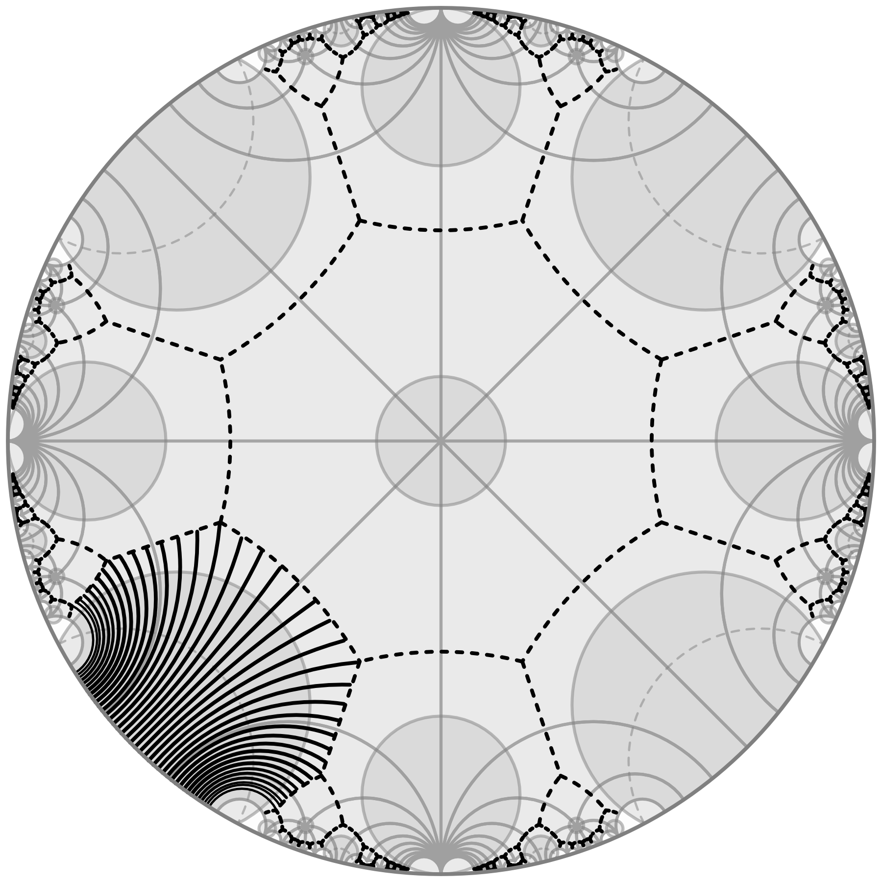
Figure 12. Depicted is the covering of the decorated hyperbolic surface discussed in Figure 1 and the $1$-skeleton of its weighted Voronoi decomposition (dashed lines). Each Voronoi $2$-cell $P_{v}$ without $V$ is homeomorphic to a once punctured disc. This can be seen by considering the “polar coordinates” $(p,t)\mapsto\gamma_{p}^{v}(t)$ introduced in Lemma 3.10. The solid black segments are a sampling of their “radial coordinate lines”.

Lemma 3.11.

There is only a finite number of Voronoi $0$-cells each of which is a point.

Proof.

Let $p\in\Sigma$ be a point contained in a Voronoi $0$-cell. We can find a circular disc $D\subset\mathbb{H}$ and an isometry $\varphi\colon D\to\Sigma$ such that $\varphi^{-1}(p)\eqcolon\tilde{p}$ is the centre of $D$. By definition, there are $N\geq 3$ geodesic arcs $\gamma_{n}\colon(0,1)\to\Sigma$ corresponding to the minimisers of $\operatorname{td}_{p}$ in $\{C_{v}\}_{v\in V}$. Suppose they are enumerated in counter-clockwise direction. These geodesic arcs are pulled back by $\varphi$ to the intersections of $D$ with hyperbolic rays starting at $\tilde{p}$ (see Figure 13). Let $v_{n}\in V$ be the endpoint of $\gamma_{n}$. Then there is a hyperbolic cycle $C_{n}$ of type $\epsilon_{v_{n}}$ and radius $r_{v_{n}}$ on the ray corresponding to $\gamma_{n}$ such that $\operatorname{td}_{p}(C_{v_{n}})=\operatorname{td}_{\tilde{p}}(C_{n})$. Maybe after choosing a smaller disc $D$, it follows that $\operatorname{td}_{\varphi(x)}(C_{v_{n}})=\operatorname{td}_{x}(C_{n})$ for all $x\in D$ and $n=1,\dotsc,N$, because $\operatorname{dist}_{\Sigma}$ is continuous. Hence, $\tilde{p}$ is the common intersection point of the radical lines of consecutive cycles $C_{n}$ (see Lemma 2.13). Due to the requirement of properness of the decoration consecutive radical lines can not coincide. This shows that the set of Voronoi $0$-cells consists of isolated points. Observing that all $0$-cells have to be contained in the compact set $\Sigma^{\prime}$ constructed in Lemma 3.10, we see that there are only a finite number of Voronoi $0$-cells. ∎

Figure 13. Using a small isometrically embedded disc $(\varphi,D)$ about a point $p\in\Sigma$ contained in a Voronoi $0$-cell, we can pull back the $\operatorname{td}$-minimising cycles along hyperbolic rays (solid black) corresponding to the geodesic arcs in $\Sigma$. It follows that $p$ is an isolated point since $\tilde{p}\coloneq\varphi^{-1}(p)$ is the common intersection point of the radical lines (dashed black) of consecutive cycles.

Theorem 3.12 (dual tessellation of weighted Voronoi decomposition).

Let $\Sigma^{\omega}$ be a properly decorated hyperbolic surface. The combinatorial dual of its weighted Voronoi decomposition can be realised as a geodesic tessellation of $\Sigma$. This realisation exhibits the following properties:

1. If the vertex discs of the decoration do not intersect, the realisation is given by the weighted Delaunay tessellation of $\Sigma^{\omega}$ (Definition 3.3). In particular, the Voronoi $0$-cells are the centres of the properly immersed discs defining the Delaunay $2$-cells.

2. All edges of a geodesic triangulation refining the realisation satisfy the local Delaunay condition (Definition 2.19). In particular, an edge satisfies the strict local Delaunay condition iff it already was an edge of the weighted Delaunay tessellation.

Figure 14. Visualisation of the constructions used in Theorem 3.12. Left: building upon the construction presented in Lemma 3.11, we can associate a hyperbolic polygon $P$ (shaded) to a Voronoi $0$-cell. The embedding $\varphi$ can be extended to an isometric immersion using the indicated homotopy. Right: should some cone-point $\Phi(q)$ obstruct extending $\varphi$ to all of $\operatorname{int}(P)$ then $\operatorname{td}_{p}(C_{v_{n}})>\operatorname{td}_{p}(C_{\Phi(q)})$ as $q$ and $\tilde{p}$ lie on the same side of the radical line (dashed black) between $C_{n}$ and $q$.

Proof.

Consider a Voronoi $0$-cell $p\in\Sigma$. Let $\varphi\colon D\to\Sigma$ be the isometry and $C_{1},\dotsc,C_{N}$ be the hyperbolic cycles defined in Lemma 3.11. In addition to the $C_{n}$ we can find hyperbolic cycles $S_{n}$ corresponding to the $S_{v}$ defined in Lemma 3.10. By construction their associated discs do not intersect. Let $P\coloneq\operatorname{poly}(S_{1},\dotsc,S_{N})$. We show that the interior of $P$ can be isometrically mapped into $\Sigma$, i.e., it defines an (open) Delaunay $2$-cell. The rest of the assertions, including properties (i) and (ii), follow directly by tracing back the definitions made up to this point.

All cycles $C_{n}$ have equal tangent distance to $\tilde{p}\coloneq\varphi^{-1}(p)$. Hence, we find an $F\in\operatorname{Sym}(2)$ such that $\langle F,C_{n}\rangle=-1$ for all $n=1,\dotsc,N$. Indeed, $F=\tilde{p}/\operatorname{td}_{\tilde{p}}(C_{n})$. Note that $F$ defines a properly immersed disc if $|F|^{2}>-1$. Furthermore, the $C_{n}$ give another decoration of $P$ as $C_{n}$ and $S_{n}$ share the same centre. So Proposition 2.18 grants that the centres of the $C_{n}$ are exactly the vertices of $P$. Consider the cycles $C_{1}$ and $C_{2}$. We can homotope the path given by the concatenation of the two rays connecting $\tilde{p}$ with $C_{1}$ and $C_{2}$, respectively, to the edge between these cycles by moving $\tilde{p}$, and with it the rays, along the radical line of $C_{1}$ and $C_{2}$ (see Figure 14, left). Proceeding like this for all consecutive cycles $C_{n}$ and $C_{n+1}$ we can extend $\varphi$ to an isometric immersion $\Phi\colon U\to\Sigma$. Here, $U\subseteq P$ shall be the largest set which can be obtained by the described homotopy such that $\Phi$ is still isometric. Suppose that $U\neq P$. Then there is a $q\in\partial U$ with $q\in\operatorname{int}(P)$ and $\Phi(q)\in V_{-1}$. Let $C_{n}$ be a cycle whose centre has minimal distance to $q$. Then the angle at $q$ between the rays connecting it to $\tilde{p}$ and the centre of $C_{n}$ is $>\pi/2$ (see Figure 14, right). Thus, by the properness of the decoration and Corollary 2.14, we see that

$$\operatorname{td}_{\tilde{p}}(C_{n})\;>\;\frac{\cosh(\operatorname{dist}_{\mathbb{H}}(q,\tilde{p}))}{\cosh(r_{\Phi(q)})}\;>\;\operatorname{td}_{p}(C_{\Phi(q)}).$$

This contradicts the minimality of $\operatorname{td}_{p}(C_{v_{n}})=\operatorname{td}_{\tilde{p}}(C_{n})$. So $U=P$. Finally, suppose $\Phi|_{\operatorname{int}(P)}$ is not injective. Similarly to Lemma 3.5, we can find a non-trivial hyperbolic motion $M$ such that $P\cap M(P)\neq\emptyset$ and $\Phi|_{P\cap M(P)}=(\Phi\circ M^{-1})|_{P\cap M(P)}$. Since $\Phi|_{\operatorname{int}(P)}$ is an isometry on each region belonging to a Voronoi $2$-cell (Lemma 3.10) we see that there is no neighbourhood of $\tilde{p}$ over which $\Phi$ is injective. But this contradicts the initial assertion that $\Phi|_{D}$ is an isometry. It follows that $\Phi$ is injective over $\operatorname{int}(P)$. ∎

This theorem justifies the following generalisation of the notion of weighted Delaunay tessellation to properly decorated surfaces.

Definition 3.13 (weighted Delaunay tessellation, proper decorations).

For a properly decorated surface $\Sigma^{\omega}$ the geodesic tessellation dual to the weighted Voronoi decomposition of $\Sigma^{\omega}$ is called weighted Delaunay tessellation of $\Sigma^{\omega}$. A geodesic triangulation refining this tessellation is called a weighted Delaunay triangulation of $\Sigma^{\omega}$.

3.4. The flip algorithm

Consider a geodesic triangulation $T$ of a properly decorated hyperbolic surface $\Sigma^{\omega}$. A triangle $\Delta$ of $T$ can be lifted to a decorated triangle in $\mathbb{H}$. This lift is not unique but any two lifts can be connected by a hyperbolic motion. Denote the vertex cycles of some lift by $C_{1}$, $C_{2}$ and $C_{3}$. Furthermore, let $F_{\Delta}\in\operatorname{Sym}(2)$ denote their face-vector. The support function $H_{\Delta}^{\omega}\colon\mathbb{H}\setminus\{\langle X,F_{\Delta}\rangle=0\}\to\mathbb{R}_{>0}$ of the decorated triangle $\Delta$ is defined by

$$-1\;=\;\big{\langle}\sqrt{\smash[b]{H_{\Delta}^{\omega}(X)}}\,X,\,F_{\Delta}\big{\rangle}$$

for all $X\in\mathbb{H}\setminus\{\langle X,F_{\Delta}\rangle=0\}$. We observe that $\operatorname{poly}(C_{1},C_{2},C_{3})\subset\mathbb{H}\setminus\{\langle X,F_{\Delta}\rangle=0\}$ because $\langle C_{n},F_{\Delta}\rangle=-1$. Hence, $H_{\Delta}^{\omega}$ is well defined on $\Delta\subset\Sigma$. For two adjacent triangles the support functions agree on their common edge (see Figure 15). It follows, that each geodesic triangulation $T$ of a decorated hyperbolic surface $\Sigma^{\omega}$ induces a continuous support function $H_{T}^{\omega}\colon\Sigma\to\mathbb{R}_{>0}$ restricting to $H_{\Delta}^{\omega}$ on each triangle $\Delta$, respectively.

Figure 15. Decorating a hyperbolic triangle $\Delta$ defines a lift to the affine plane $\{\langle F_{\Delta},X\rangle=-1\}\subset\operatorname{Sym}(2)$. The support function $H^{\omega}_{\Delta}$ is given by the scaling factors such that $\sqrt{\smash[b]{H_{\Delta}^{\omega}(X)}}X\in\{\langle F_{\Delta},X\rangle=-1\}$ for all $X\in\mathbb{H}\setminus\{\langle F_{\Delta},X\rangle=0\}$. If two decorated triangles $\Delta$ and $\tilde{\Delta}$ share an edge, then their support functions agree on the corresponding points.

Theorem 3.14 (flip algorithm).

Let $\Sigma^{\omega}$ be a properly decorated hyperbolic surface. Start with any geodesic triangulation of $\Sigma$. Then consecutively flipping edges violating the strict local Delaunay condition terminates after a finite number of steps. The computed triangulation of $\Sigma$ is a weighted Delaunay triangulation with respect to the decoration $\omega$ in the sense of Theorem 3.12.

Proof.

Let us suppose for a moment that consecutively flipping edges of a geodesic triangulation violating the strict local Delaunay condition terminates after a finite number of steps. Hence, all edges of the final geodesic triangulation satisfying the local Delaunay condition. Therefore, Proposition 3.21 grants that this triangulation refines the weighted Delaunay tessellation of the decorated hyperbolic surface $\Sigma^{\omega}$, i.e., it is a weighted Delaunay triangulation of $\Sigma^{\omega}$.

It remains to show that the flip algorithm terminates. Proposition 2.26 together with Example 2.25 guarantees that an edge violating the strict local Delaunay condition can always be flipped. Let $T$ and $\tilde{T}$ be geodesic triangulations. Suppose $\tilde{T}$ can be obtained from $T$ by flipping an edge $e\subset\Sigma$ of $T$ which violates the strict local Delaunay condition. Locally this is equivalent to changing to the lower convex hull of four points in $\operatorname{Sym}(2)$ (compare to the proof of Proposition 2.26). Thus we deduce that $H_{\tilde{T}}^{\omega}\leq H_{T}^{\omega}$. In particular, $H_{\tilde{T}}^{\omega}(x)<H_{T}^{\omega}(x)$ for all $x\in e$. Finally, Lemma 3.18 yields that there is an upper bound for the lengths of the edges of $T$ only determined by $H_{T}^{\omega}$ and the vertex radii. Using Lemma 3.2, it follows that there is only a finite number of geodesic triangulations of $\Sigma$ whose edges satisfy this lengths constraint. This implies that the number of geodesic triangulations $\tilde{T}$ with $H_{\tilde{T}}^{\omega}\leq H_{T}^{\omega}$ is finite. ∎

Corollary 3.15.

Let $T$ be a weighted Delaunay triangulation of a properly decorated hyperbolic surface $\Sigma^{\omega}$. Then $H_{T}^{\omega}\leq H_{\tilde{T}}^{\omega}$ for any other geodesic triangulation $\tilde{T}$ of $\Sigma$. In particular $H_{T}^{\omega}=H_{\tilde{T}}^{\omega}$ holds iff $\tilde{T}$ is another weighted Delaunay triangulation of $\Sigma^{\omega}$.

Corollary 3.16 (generalised Epstein-Penner convex hull construction).

Let $\Sigma^{\omega}$ be a properly decorated hyperbolic surface coming from a finitely generated, non-elementary Fuchsian group $\Gamma<\operatorname{PSL}(2;\mathbb{R})$ (see Example 3.1). Since the covering space of $\Sigma$ is $\mathbb{H}$, we can find for each vertex $v\in V$ an orbit $\mathcal{C}_{v}\coloneq\{C_{v}^{g}\}_{g\in\Gamma}\subset\operatorname{Sym}(2)$, each element representing the vertex cycle about $v$ (see Proposition 2.6). Then the boundary of $\operatorname{conv}\left(\bigcup_{v\in V}\mathcal{C}_{v}\right)$ exhibits the following properties:

• it consists of a countable number of codimension-one “faces” each of which is the convex hull of a finite number of points in $\bigcup_{v\in V}\mathcal{C}_{v}$,

• each face lies in an elliptic plane, i.e, its face-vector $F$ satisfies $|F|^{2}<0$,

• the set of faces is locally finite about each point in $\bigcup_{v\in V}\mathcal{C}_{v}$,

• the set of faces can be partitioned into a finite number of $\Gamma$-invariant subsets,

• the faces project to the Delaunay $2$-cells of the decorated hyperbolic surface.

The rest of the section is devoted to proving the technical details needed for the proof of Theorem 3.14. We begin by analysing the relation between the function $H_{T}^{\omega}$ and the edge-lengths.

Lemma 3.17.

Suppose $C_{0},C_{1}\in\operatorname{Sym}(2)$ are two hyperbolic cycles in $\mathbb{H}$ whose corresponding discs do not intersecting. Then $|C_{1}-C_{0}|^{2}>0$ and

$$0\,<\,\operatorname*{argmin}_{\lambda\in\mathbb{R}}|C_{0}+\lambda(C_{1}-C_{0})|^{2}\,<\,1.$$

Proof.

Let $\hat{C}_{0}$ and $\hat{C}_{1}$ be the lifts of $C_{0}$ and $C_{1}$ to $\operatorname{Herm}(2)$ as defined in Proposition 2.6, respectively. From Lemma 2.13 follows that $C_{0}$ and $C_{1}$ posses a radical line. By Lemma 2.4, this radical line is given by $\hat{C}_{1}-\hat{C}_{0}=C_{1}-C_{0}$ since it is contained in the pencil spanned by $\hat{C}_{0}$ and $\hat{C}_{1}$. Hence $|C_{1}-C_{0}|^{2}>0$ as $C_{1}-C_{0}$ is a Möbius-circle. Furthermore, the cycles lie on different sides of the radical line, i.e., $\langle C_{0},C_{1}-C_{0}\rangle<0$ and $\langle C_{1},C_{1}-C_{0}\rangle>0$, because their discs do not intersect. It follows that

$$|C_{1}-C_{0}|^{2}\,=\,\langle C_{1},C_{1}-C_{0}\rangle\,-\,\langle C_{0},C_{1}-C_{0}\rangle\,>\,-\langle C_{0},C_{1}-C_{0}\rangle.$$

Finally, the expression $|C_{0}+\lambda(C_{1}-C_{0})|^{2}$ is quadratic in $\lambda$. Thus its minimum point is given by the root of the first derivative, that is,

$$\lambda_{\mathrm{min}}\,=\,-\frac{\langle C_{0},C_{1}-C_{0}\rangle}{|C_{1}-C_{0}|^{2}}.\qed$$

Lemma 3.18.

Let $\Delta\subset\Sigma$ be a triangle in a geodesic triangulation $T$ of a properly decorated hyperbolic surface $\Sigma^{\omega}$. Suppose it is incident to the vertices $v_{0},v_{1},v_{2}\in V$ and define $H_{\Delta,\omega}^{\max}\coloneq\max\{1,\,\max_{x\in\Delta}H_{T}^{\omega}(x)\}.$ Then the edge-lengths of the edges of $\Delta$ are bounded from above by

$$\max\big{\{}r_{v_{m}}+r_{v_{n}}+2\operatorname{arcosh}(H^{\max}_{\Delta,\omega})\;:\;m,n\in\{0,1,2\}^{2},\;m<n\big{\}}.$$

Proof.

Consider two vertices, say $v_{0}$ and $v_{1}$. Lift the edge between $v_{0}$ and $v_{1}$ to $\mathbb{H}$. Denote by $C_{0}$ and $C_{1}$ the corresponding lifts of the vertex cycles. If the cycles $C_{0}$ and $C_{1}$ intersect, then the length of the edge between them is less or equal to $r_{v_{0}}+r_{v_{1}}$. Now assume otherwise. The previous Lemma 3.17 shows that $h_{01}\coloneq-\min_{\lambda\in\mathbb{R}}|C_{0}+\lambda(C_{1}-C_{0})|^{2}\leq H^{\max}_{\Delta,\omega}.$ In addition, the pencil spanned by the cycles contains two points. The distance of these points bounds the distance of the cycles since each of the discs bounded by the cycles contains one of them. One computes that the distance of the points is given by $2\operatorname{arcosh}(h_{01})$. The monotonicity of the $\operatorname{arcosh}$-function yields the result. ∎

Finally, we are going to consider the relationship between the support function $H_{T}^{\omega}$, the local Delaunay condition and global Delaunay triangulations. The following proposition proves the ellipticity part of Corollary 3.16. This provides us with the means to derive some technical details about the geometry of support functions (Lemma 3.20) building the core of the proof of Proposition 3.21.

Proposition 3.19.

Consider a geodesic triangulation $T$ of a properly decorated hyperbolic surface $\Sigma^{\omega}$. Suppose that all edges satisfy the local Delaunay condition. Then the face-vector $F_{\Delta}\in\operatorname{Sym}(2)$ of any lift of a (decorated) triangle $\Delta$ to $\mathbb{H}$ satisfies $|F_{\Delta}|^{2}<0$.

Proof.

Suppose otherwise. We are going to construct a geodesic ray $\gamma\colon[0,\infty)\to\Sigma\setminus V$ such that $H_{T}^{\omega}\circ\gamma$ is unbounded. This is a contradiction to the existence of $\max_{x\in\Sigma}H_{T}^{\omega}(x)$. There are two cases: either $|F_{\Delta}|^{2}=0$ or $|F_{\Delta}|^{2}>0$. We are only elaborating the first case. The proof for the other one works similarly.

Let $\Delta_{0}$ be a triangle whose lift $\tilde{\Delta}_{0}$ has a face-vector satisfying $|F_{\Delta_{0}}|^{2}=0$. Choose a geodesic ray $\tilde{\gamma}\colon[0,\infty)\to\mathbb{H}$ starting in the interior of $\tilde{\Delta}_{0}$ which limits to the centre of the horocycle corresponding to $F_{\Delta_{0}}$ and intersects the interior of an edge of $\tilde{\Delta}_{0}$. Maybe after perturbing the ray a little bit, it projects to a geodesic ray $\gamma\colon[0,\infty)\to\Sigma\setminus V$. Successively lift triangles of $T$ along $\gamma$ to $\mathbb{H}$ such that they cover $\tilde{\gamma}$ (see Figure 16). Denote the triangles by $\Delta_{1},\Delta_{2},\dotsc$ and the times when $\gamma$ intersects edges of $T$ by $0\eqcolon s_{0}<s_{1}<s_{2}<\cdots$. Hence, $(H_{T}^{\omega}\circ\gamma)(s)=(H_{\Delta_{n}}^{\omega}\circ\tilde{\gamma})(s)$ for $s_{n}\leq s\leq s_{n+1}$. By the local Delaunay condition (compare to Lemma 3.20), $(H_{\Delta_{m}}^{\omega}\circ\tilde{\gamma})(s)\geq(H_{\Delta_{n}}^{\omega}\circ\tilde{\gamma})(s)$ for $s>s_{n+1}$ and $m>n$. Finally, by construction, there is a $\lambda_{s}>0$ for every $s\geq 0$ such that

$$(H_{\Delta_{0}}^{\omega}\circ\tilde{\gamma})(s)\;=\;-\big{|}\sqrt{h_{0}}\,\tilde{\gamma}(0)+\lambda_{s}F_{\Delta_{0}}\big{|}^{2}\;=\;h_{0}+2\lambda_{s}\mathrm{e}^{\delta}.$$

Here $h_{0}\coloneq(H_{\Delta_{0}}^{\omega}\circ\tilde{\gamma})(0)$ and $\delta$ is the (oriented) distance of $\tilde{\gamma}(0)$ to the horocycle given by $F_{\Delta_{0}}$. Note that $\lambda_{s}\to\infty$ as $s\to\infty$. Thus, $(H_{\Delta_{0}}^{\omega}\circ\tilde{\gamma})(s)\to\infty$ as $s\to\infty$, too. ∎

Figure 16. Sketch of the construction used in Proposition 3.19.

Lemma 3.20.

Let $C$ be a hyperbolic cycle in $\mathbb{H}$ and $L$ a hyperbolic line orthogonal to it. Let $\gamma\colon\mathbb{R}\to L$ be the parametrisation of $L$ by the (oriented) distance to the (auxiliary) centre of $C$. If $C$ is a horo- or hypercycle choose $\gamma$ such that $\mathbb{R}_{<0}$ is mapped into the disc associated to $C$. Consider $F_{1},F_{2}\in\operatorname{Sym}(2)\setminus\operatorname{span}\{C\}$ with $\langle C,F_{n}\rangle=-1$, $n=1,2$, such that $\nu F_{1}$ and $\nu F_{2}$ are hyperbolic circles for some $\nu>0$. Denote by $H_{n}\colon\mathbb{H}\to\mathbb{R}$ the support function induced by $F_{n}$. Furthermore, let $\delta_{n}$ the distance of the (auxiliary) centre of $C$ to the orthogonal projection of the centre of $F_{n}$ to the line $L$ (see Figure 17).

Then the sign of $H_{1}\circ\gamma-H_{2}\circ\gamma$ is constant over $\mathbb{R}_{>0}$ if $C$ is a circle or $\mathbb{R}$ otherwise. Furthermore, if $(H_{1}\circ\gamma)(s)>(H_{2}\circ\gamma)(s)$ for some $s>0$, then $\delta_{1}>\delta_{2}$.

Proof.

The first claim about the sign follows from observing that the functions $H_{n}\circ\gamma$ correspond to two intersecting affine lines in $\operatorname{Sym}(2)$. Indeed, for each $s\in\mathbb{R}$ there is a $\lambda_{s}>0$ such that

$$\sqrt{(H_{n}\circ\gamma)(s)}\,\gamma(s)\,=\,C\,+\,\lambda_{s}X_{n}$$

where $X_{n}\coloneq\sqrt{(H_{n}\circ\gamma)(1)}\,\gamma(1)-C$, $n=1,2$, (compare to Figure 15).

Next, note that we can assume $F_{1}$, $F_{2}$ and $C$ to represent hyperbolic cycles, maybe after rescaling, i.e., considering $\nu F_{1}$, $\nu F_{2}$ and $(1/\nu)C$ for some $\nu>0$. Denote by $\epsilon\in\{-1,0,1\}$ the type of $C$ and by $R$ its radius. Furthermore, let $r_{n}>0$ denote the radius of the circle corresponding to $F_{n}$ and by $d_{n}$ the distance between its centre and $L$. Finally, consider an $s>0$ such that $\gamma(s)$ is not contained in the discs associated to $F_{1}$ and $F_{2}$. Then there are circles centred at $\gamma(s)$ orthogonally intersecting $F_{1}$ or $F_{2}$, respectively. Denote their radii by $r^{s}_{1}$ and $r^{s}_{2}$. Using Lemma 2.11 we see that $\cosh(r_{n})\tau^{\prime}_{\epsilon}(R)=\tau^{\prime}_{\epsilon}(\delta_{n})\cosh(d_{n})$ and $\cosh(r_{n})\cosh(r_{n}^{s})=\cosh(d_{n})\cosh(s-\delta_{n})$. Hence

$$\cosh(r_{n}^{s})\,=\,\frac{\tau^{\prime}_{\epsilon}(R)\cosh(s-\delta_{n})}{\tau^{\prime}_{\epsilon}(\delta_{n})}.$$

By Lemma 2.9, $(H_{n}\circ\gamma)(s)=\cosh^{-2}(r_{n}^{s})$. Therefore, assuming that $(H_{1}\circ\gamma)(s)>(H_{2}\circ\gamma)(s)$ is equivalent to

(28) $$\frac{\mathrm{e}^{\delta_{2}}+\epsilon\mathrm{e}^{-\delta_{2}}}{\mathrm{e}^{\delta_{1}}+\epsilon\mathrm{e}^{-\delta_{1}}}\;<\;\mathrm{e}^{\delta_{1}-\delta_{2}}\frac{1+\mathrm{e}^{2(\delta_{2}-s)}}{1+\mathrm{e}^{2(\delta_{1}-s)}}.$$

Here we used that $\tau^{\prime}_{\epsilon}(x)=(\mathrm{e}^{x}+\epsilon\mathrm{e}^{-x})/2$. After taking the limit $s\to\infty$ and rearranging we arrive at $\delta_{1}\geq\delta_{2}$. But equation (28) prohibits equality. ∎

Figure 17. Sketch of the geometric objects considered in Lemma 3.20. It shows elements of two distinct pencils of cycles which both contain a hyperbolic cycle $C$ and their dual pencils both contain a common hyperbolic line $L$. The radical line of the first pencil intersects $L$ further to the right then the radical line of the second pencil, i.e., $\delta_{1}>\delta_{2}$, if at some point $\gamma(s)\in L$ the radii of the corresponding members of the pencils satisfy $r_{2}^{s}>r_{1}^{s}$, that is, $(H_{1}\circ\gamma)(s)>(H_{2}\circ\gamma)(s)$.

Proposition 3.21.

Let $T$ be a geodesic triangulation of a properly decorated hyperbolic surface $\Sigma^{\omega}$ whose edges all satisfy the local Delaunay condition. Then it refines the weighted Delaunay tessellation of $\Sigma^{\omega}$.

Proof.

Let $\tilde{T}$ be another geodesic triangulation whose edges all satisfy the local Delaunay condition. We claim that an edge of $T$ is either also an edge of $\tilde{T}$ or it only intersects edges of $\tilde{T}$ which satisfy the local Delaunay condition with equality. The proposition now follows from the properties of the weighted Delaunay tessellation (Theorem 3.12 item (ii)).

We proceed by proving the claim. Let $e$ be an edge of $T$ incident to the vertices $u,v\in V$. Denote by $\gamma\colon I\to e$ the parametrisation of $e$ by the (oriented) distance to the centre of $C_{u}$. If $C_{u}$ is a horo- or hypercycle choose $\gamma$ such that $\mathbb{R}_{<0}$ is mapped into the disc associated to $C_{u}$. Suppose that $e$ intersects $N>0$ edges of $\tilde{T}$ at $(s_{n})_{1\leq n\leq N}\subset I$ with

$$\inf I\eqcolon s_{0}\;<\;s_{1}\;<\;\cdots\;<\;s_{N}\;<\;s_{N+1}\coloneq\sup I.$$

By definition, $h\coloneq H_{T}^{\omega}\circ\gamma$ is a function satisfying the assumptions of Lemma 3.20 whilst $\tilde{h}\coloneq H_{\tilde{T}}^{\omega}\circ\gamma$ is a continuous function agreeing on each $(s_{n},s_{n+1})$ with such a function $\tilde{h}_{n}\colon I\to\mathbb{R}$. Towards a contradiction, suppose that there is an $x\in I$ such that $\tilde{h}(x)=\tilde{h}_{n}(x)>h(x)$. After possibly changing the role of $u$ and $v$, from Lemma 3.20 follows that $\tilde{h}_{n}(s)>h(s)$ for all $s<x$. Using the local Delaunay condition, we see by induction that $\tilde{h}_{m}(s)\geq\tilde{h}_{n}(s)$ for all $s<s_{m+1}$ and $m<n$. Hence, $\tilde{h}_{0}(s)>h(s)$ for all $s<s_{1}$. Utilising Lemma 3.20 and the local Delaunay condition one more time we get

(29) $$\delta\;<\;\tilde{\delta}_{0}\;<\;\cdots\;<\;\tilde{\delta}_{N}$$

and $\tilde{h}_{N}(s)>h(s)$ for all $s>s_{N}$. Considering the parametrisation of $e$ with respect of $C_{v}$ instead of $C_{u}$, the second inequality and Lemma 3.20 imply $\ell_{e}-\delta<\ell_{e}-\tilde{\delta}_{N}$. Here $\ell_{e}$ is the length of the edge $e$. But this is equivalent to $\tilde{\delta}_{N}<\delta$ contradicting inequality (29). Thus, $h(s)\geq\tilde{h}(s)$ for all $s\in I$. Applying the same argument to each edge of $\tilde{T}$ which intersects $e$ we also get $h(s_{n})\leq\tilde{h}(s_{n})$, $n=1,\dotsc,N$. It follows $h(s)=\tilde{h}(s)$ for all $s\in I$. This is equivalent to the claim. ∎

4. The configuration space of decorations

Recall that the weight-vector of a decoration is defined as $\omega\coloneq(\tau_{\epsilon_{v}}(r_{v}))_{v\in V}\in\mathbb{R}_{>0}^{V}$. We call $\mathbb{R}_{>0}^{V}$ the space of abstract (positive) weights. Its subspace $\mathfrak{D}_{\Sigma}\subseteq\mathbb{R}_{>0}^{V}$ consisting of all weight-vectors $\omega\in\mathbb{R}_{>0}^{V}$ satisfying the homogeneous linear constraints

(30) $$0\;>\;\omega_{v}\,-\,\tau_{\epsilon_{v}}(\operatorname{dist}_{\Sigma}(v,\tilde{v}))\,\omega_{\tilde{v}}$$

for all $(v,\tilde{v})\in V\times V_{-1}$ is the configuration space of proper decorations of $\Sigma$. If $V_{-1}=\emptyset$ all abstract weights can be realised as the (modified) radii of decoration of $\Sigma$. Furthermore, it is clear that $\mathfrak{D}_{\Sigma}=\mathbb{R}_{>0}^{V}$. For $V_{-1}=\emptyset$ weights in $\mathfrak{D}_{\Sigma}$ can, in general, only be realised as a decoration of $\Sigma$ if $\omega_{v}<\tau_{\epsilon_{v}}(\operatorname{dist}_{\Sigma}(v,\tilde{v}))$ and $1<\omega_{\tilde{v}}$ for all $(v,\tilde{v})\in V\times V_{-1}$. Still, the derivations of the previous sections 3.3 and 3.4 are true for all weights in $\mathfrak{D}_{\Sigma}$, since the key observation, i.e., Corollary 2.14, only depends on the constraints (30). In particular, for any $\omega\in\mathfrak{D}_{\Sigma}$ Theorem 3.12 grants the existence of a unique weighted Delaunay tessellation with respect to the decoration induced by $\omega$. Denote it by $T_{\Sigma}^{\omega}$. Let $T$ be some geodesic tessellation of $\Sigma$. We define

$$\mathfrak{D}_{\Sigma}(T)\;\coloneq\;\big{\{}\omega\in\mathfrak{D}_{\Sigma}\,:\,T\text{ refines }T_{\Sigma}^{\omega}\big{\}}.$$

Note that $\mathfrak{D}_{\Sigma}(T)$ is allowed to be empty.

Lemma 4.1.

Consider the weighted Delaunay tessellation $T_{\Sigma}^{\omega}$ corresponding to $\omega\in\mathfrak{D}_{\Sigma}$. Then $\mathfrak{D}_{\Sigma}(T_{\Sigma}^{\omega})$ is the intersection of $\mathfrak{D}_{\Sigma}$ with a closed polyhedral cone $\mathcal{C}_{\Sigma}(T_{\Sigma}^{\omega})$. Furthermore, the faces of $\mathcal{C}_{\Sigma}(T_{\Sigma}^{\omega})$ are exactly given by those cones $\mathcal{C}_{\Sigma}(T_{\Sigma}^{\tilde{\omega}})$ defined by weighted Delaunay tessellations $T_{\Sigma}^{\tilde{\omega}}$ which $T_{\Sigma}^{\omega}$ refines.

Proof.

Let $T$ be a geodesic triangulation refining $T_{\Sigma}^{\omega}$. Then all edges of $T$ satisfy the local Delaunay condition (Theorem 3.12). We observe that the tilts (Definition 2.23), and thus the local Delaunay condition (Proposition 2.24), are linear in the $\tau_{\epsilon_{v}}(r_{v})=\omega_{v}$. It follows that $\mathcal{C}_{\Sigma}(T_{\Sigma}^{\omega})$ is the solution space to a finite number of homogeneous linear inequalities and equalities, thus a closed polyhedral cone. The second claim about the faces of $\mathcal{C}_{\Sigma}(T_{\Sigma}^{\omega})$ is a reformulation of Theorem 3.12 item (ii). ∎

Corollary 4.2.

Let $\omega\in\mathfrak{D}_{\Sigma}$. Then $\{s\omega:s>0\}\subseteq\mathfrak{D}_{\Sigma}(T_{\Sigma}^{\omega}).$ In particular, for any geodesic triangulation $T$ refining $T_{\Sigma}^{\omega}$ we have $H_{T}^{s\omega}=(1/s^{2})H_{T}^{\omega}$. Here $H_{T}^{\omega}$ and $H_{T}^{s\omega}$ are the support functions induced by $\omega$ and $s\omega$, respectively.

Theorem 4.3 (configuration space of proper decorations).

The configuration space $\mathfrak{D}_{\Sigma}$ of proper decorations of $\Sigma$ is a convex connected subset of $\mathbb{R}_{>0}^{V}$. There is only a finite number of geodesic tessellations $T_{1},\dotsc,T_{N}$ such that $\mathfrak{D}_{\Sigma}(T_{n})$ are non-empty. In particular, $\mathfrak{D}_{\Sigma}=\bigcup_{n}\mathfrak{D}_{\Sigma}(T_{n})$. In addition, for all $1\leq m<n\leq N$ either $\mathfrak{D}_{\Sigma}(T_{m})\cap\mathfrak{D}_{\Sigma}(T_{n})=\emptyset$ or there is a $k\neq m,n$ such that $\mathfrak{D}_{\Sigma}(T_{m})\cap\mathfrak{D}_{\Sigma}(T_{n})=\mathfrak{D}_{\Sigma}(T_{k})$.

Proof.

Everything except the (global) finiteness of the decomposition was covered in Lemma 4.1. Aiming for a contradiction, suppose that there are infinitely many geodesic tessellations $(T_{n})_{n=1}^{\infty}$ with $\mathfrak{D}_{\Sigma}(T_{n})\neq\emptyset$. In particular, we assume that $T_{m}\neq T_{n}$ if $m\neq n$. Denote by $\SS^{V}\coloneq\{\omega\in\mathbb{R}^{V}:\sum_{v\in V}\omega_{v}^{2}=1\}$ the unit sphere in $\mathbb{R}^{V}$. Choose for each $n\geq 1$ a $\omega^{n}\in\SS^{V}\cap\mathfrak{D}_{\Sigma}(T_{n})$. Then there is a convergent subsequence of $(\omega^{n})_{n=1}^{\infty}$ since $\SS^{V}$ is compact. To simplify notation, we assume that $(\omega^{n})_{n=1}^{\infty}$ already converges. Let $\omega\in\mathbb{R}_{\geq 0}^{V}\cap\SS^{V}$ be its limit point. Denote by $V_{0}^{0}$ and $V_{1}^{0}$ those vertices $v$ in $V_{0}$ or $V_{1}$ with $\omega_{v}=0$, respectively. Note that by construction $V_{0}^{0}\cup V_{1}^{0}\neq V$.

First, assume that $V_{0}^{0}\cup V_{1}^{0}=\emptyset$. If $\omega\in\mathfrak{D}_{\Sigma}$, it induces a weighted Delaunay tessellation by Corollary 4.2. This contradicts the local finiteness of the decomposition implied by Lemma 4.1. Should $\omega\in\partial\mathfrak{D}_{\Sigma}$ instead, then $\operatorname{td}_{x}(\omega_{v}^{n})\coloneq\tau_{\epsilon_{v}}(\operatorname{dist}_{\Sigma}(v,x))/\omega_{v}^{n}$ still converges for all $x\in\Sigma$ and $v\in V$ as $n\to\infty$. So the global finiteness follows again from the local finiteness. Now assume $V_{0}^{0}\cup V_{1}^{0}\neq\emptyset$. The idea is to show that the (combinatorial) star of each vertex in $V_{0}^{0}\cup V_{1}^{0}$ is constant for large enough $n$. Then we can use the same argument as in the first case. To this end, consider the auxiliary sequence $(\tilde{\omega}^{n})_{n=1}^{\infty}$ with

$$\tilde{\omega}_{v}^{n}\;\coloneq\;\begin{cases}\omega_{v}^{n}&,\text{if }v\in V_{0}^{0}\cup V_{1}^{0},\\ \omega_{v}&,\text{otherwise}.\end{cases}$$

In the weighted Voronoi decomposition dual to the weighted Delaunay tessellation $T_{\Sigma}^{\tilde{\omega}^{n}}$ to each vertex $v$ corresponds an open Voronoi $2$-cell $P_{v}^{n}$ containing it. Denote its closure by $\bar{P}_{v}^{n}$. The boundary of $P_{v}^{n}$ is comprised of Voronoi $1$- and $0$-cells. By definition, for each (open) $1$-cell $e\subset\partial P_{v}^{n}$ there is a unique $u\in V$ such that $\operatorname{td}_{x}(\tilde{\omega}_{u}^{n})=\operatorname{td}_{x}(\tilde{\omega}_{v}^{n})$ for all $x\in e$. Remember the embedded cycle $S_{v}$ and the map $\gamma^{v}\colon p\mapsto\gamma_{p}^{v}(L_{p})$ introduced in Lemma 3.10. The latter maps $S_{v}$ continuously onto $\partial P_{v}^{n}$. Using this map, the Voronoi $1$-cells induce a decomposition of $S_{v}$ into segments. Hence, traversing $S_{v}$ in counter-clockwise direction, we can associate to each vertex $v$ and step $n$ a finite sequence $U_{v}^{n}\coloneq(u_{1}^{v,n},\dotsc,u_{i_{v,n}}^{v,n})$ of vertices corresponding to Voronoi $1$-cells in the boundary of $P_{v}^{n}$. Note that $U_{v}^{n}$ is defined up to cyclic permutations and that it determines the star of $v$ in $T_{\Sigma}^{\tilde{\omega}^{n}}$ together with $\gamma^{v}$. We observe that $\operatorname{td}_{x}(\tilde{\omega}_{v}^{n})\to\infty$ as $n\to\infty$ for all pairs $(x,v)\in\operatorname{trunc}(\Sigma)\times(V_{0}^{0}\cup V_{1}^{0})$. So for large enough $n$ all faces of $T_{\Sigma}^{\tilde{\omega}^{n}}$ contain at most one vertex from $V_{0}^{0}\cup V_{1}^{0}$, counted with multiplicity. Moreover the discs $D_{v}(\tilde{\omega}^{n})$ about $v\in V_{0}^{0}\cup V_{1}^{0}$ corresponding to $\tilde{\omega}^{n}$ exist for large $n$. From these observations and the definition of the modified tangent distance (Definition 2.12) follows that for each $n$ and $v\in V_{0}^{0}\cup V_{1}^{0}$ there is an $N_{v}^{n}>0$ such that $\bar{P}_{v}^{m}\subset D_{v}(\tilde{\omega}^{n})$ for all $m>N_{v}^{n}$. Conversely, there is an $M_{v}^{n}>0$ such that $D_{v}(\tilde{\omega}^{m})\subset\bar{P}_{v}^{n}$ for all $m>M_{v}^{n}$. It follows that we can find for each $n$ an $N^{n}>0$ such that $\bar{P}_{v}^{m}\subset\bar{P}_{v}^{n}$ for all $v\in V_{0}^{0}\cup V_{1}^{0}$ and $m>N^{n}$. Thus $U_{v}^{m}$ is a subsequence of $U_{v}^{n}$. We conclude that there is some $N>0$ such that $U_{v}^{n}=U_{v}^{m}$ for all $v\in V_{0}^{0}\cup V_{1}^{0}$ and $n,m>N$. ∎

Remark 4.1.

This theorem shows that the notion of a partial decoration can be extended from hyperbolic cusp surfaces to hyperbolic surfaces of finite type. For more information on partial decorations of cusp surfaces see [Springborn20]*§5.

Corollary 4.4.

The configuration space of proper decorations $\mathfrak{D}_{\Sigma}$ can be identified up to scaling with the interior of a convex $(|V|-1)$-polytope $\mathcal{P}_{\Sigma}$ contained in the standard simplex $\Delta^{|V|-1}=\operatorname{conv}\{(\delta_{v\tilde{v}})_{\tilde{v}\in V}\}_{v\in V}.$ Here $\delta_{v\tilde{v}}$ is the Kronecker-delta. The weight-vectors can be recovered using barycentric coordinates with respect to $\Delta^{|V|-1}$. In particular, $\mathcal{P}_{\Sigma}=\Delta^{|V|-1}$ if $V_{-1}=\emptyset$. Moreover, there is a (finite) simplicial decomposition of $\mathcal{P}_{\Sigma}$ such that each facet contains all points which induce the same weighted Delaunay decomposition of $\Sigma$.

Figure 18. A maximally symmetric hyperbolic quadrilateral (shaded). Its opposite edges can be identified (indicated by arrows) to obtain a hyperbolic torus with a single flare. By symmetry all vertex cycles of the quadrilateral are orthogonal to a common circle (dashed circle). Consequently the corresponding weighted Delaunay tessellation (solid edges) of the hyperbolic surface possesses only a single $2$-cell and the weighted Voronoi decomposition (dashed edges) only a single $0$-cell, respectively.

Example 4.5.

It is worth noting that a geodesic tessellation $T$ defining a $|V|$-dimensional set $\mathfrak{D}_{\Sigma}(T)\subset\mathbb{R}_{>0}^{V}$ is not always a triangulation. To see this consider a maximally symmetric hyperbolic quadrilateral (see Figure 18). Necessarily its vertices all have the same type and all its edges have the same length. We can glue opposite edges of the quadrilateral to obtain a genus-$1$ hyperbolic surface $\Sigma$ with a single vertex. By symmetry, for any non self-intersecting decoration of the quadrilateral, all vertex cycles posses a single common orthogonal circle. It follows that the corresponding weighted Delaunay tessellation $T$ possesses only a single Delaunay $2$-cell, the interior of the initial quadrilateral. Hence, $\mathfrak{D}_{\Sigma}(T)=\mathfrak{D}_{\Sigma}$.

Example 4.6.

Let $\Gamma<\operatorname{PSL}(2;\mathbb{R})$ be a non-elementary free Fuchsian group with finite-sided fundamental domain. Denote by $V$ the vertex set of the hyperbolic surface $\Sigma\coloneq\mathbb{H}/\Gamma$. Note that $V_{-1}=\emptyset$. Extend the vertex set by some $p\in\operatorname{trunc}(\Sigma)$. Then the weighted Voronoi decomposition for the “undecorated” surface, i.e., $\omega_{v}=0$ for $v\in V$ and $\omega_{p}=1$, exists by Theorem 4.3. Indeed, the open Voronoi $2$-cell containing $p$ is given by

$$\big{\{}x\in\operatorname{int}(\operatorname{trunc}(\Sigma))\;:\;\mathfrak{m}_{x}(p,0)=1\big{\}}.$$

In other words, it is the intersection of the interior of $\operatorname{trunc}(\Sigma)$ with the Dirichlet domain of $\Sigma$ defined by $p$ (see [Beardon83]*§9.4).

Example 4.7.

Let $n\geq 4$. The $(n,n,n)$-Triangle group is the subgroup $\Gamma<\operatorname{PSL}(2;\mathbb{R})$ of all Möbius transformations contained in the group generated by reflections in the hyperbolic triangle with three angles of $\pi/n$. It is a co-compact Fuchsian group. In particular, $\Sigma\coloneq\mathbb{H}/\Gamma$ is homeomorphic to a sphere and has three cone-points, i.e., $V=V_{-1}$ and $|V_{-1}|=3$. About each cone-point there is a cone-angle of $(2\pi)/n$ ([Beardon83]*§10.6). The sphere with three marked points admits four combinatorial triangulations. Each of them is a Delaunay triangulation of $\Sigma$ for some $\omega\in\mathfrak{D}_{\Sigma}$ (see Figure 19).

Figure 19. Depicted is the space of abstract weights for the hyperbolic surface associated to the $(4,4,4)$-Triangle group using the simplicial representation (Corollary 4.4). Weight-vectors can be recovered using barycentric coordinates $[\omega_{v_{1}}:\omega_{v_{2}}:\omega_{v_{3}}]$. The configuration space of proper decorations is highlighted. Its simplicial decomposition corresponding to weighted Delaunay tessellations of the surface is indicated.

References

- \bibselectreferences