Benchopt: Reproducible, efficient and collaborative optimization benchmarks

Abstract

Numerical validation is at the core of machine learning research as it allows to assess the actual impact of new methods, and to confirm the agreement between theory and practice. Yet, the rapid development of the field poses several challenges: researchers are confronted with a profusion of methods to compare, limited transparency and consensus on best practices, as well as tedious re-implementation work. As a result, validation is often very partial, which can lead to wrong conclusions that slow down the progress of research. We propose Benchopt, a collaborative framework to automate, reproduce and publish optimization benchmarks in machine learning across programming languages and hardware architectures. Benchopt simplifies benchmarking for the community by providing an off-the-shelf tool for running, sharing and extending experiments. To demonstrate its broad usability, we showcase benchmarks on three standard learning tasks: $\ell_{2}$-regularized logistic regression, Lasso, and ResNet18 training for image classification. These benchmarks highlight key practical findings that give a more nuanced view of the state-of-the-art for these problems, showing that for practical evaluation, the devil is in the details. We hope that Benchopt will foster collaborative work in the community hence improving the reproducibility of research findings.

1 Introduction

Numerical experiments have become an essential part of statistics and machine learning (ML). It is now commonly accepted that every new method needs to be validated through comparisons with existing approaches on standard problems. Such validation provides insight into the method’s benefits and limitations and thus adds depth to the results. While research aims at advancing knowledge and not just improving the state of the art, experiments ensure that results are reliable and support theoretical claims [128]. Practical validation also helps the ever-increasing number of ML users in applied sciences to choose the right method for their task. Performing rigorous and extensive experiments is, however, time-consuming [118], particularly because comparisons against existing methods in new settings often requires reimplementing baseline methods from the literature. In addition, ingredients necessary for a proper reimplementation may be missing, such as important algorithmic details, hyperparameter choices, and preprocessing steps [111].

In the past years, the ML community has actively sought to overcome this “reproducibility crisis” [72] through collaborative initiatives such as open datasets (OpenML, [138]), standardized code sharing [55], benchmarks (MLPerf, [99]), the NeurIPS and ICLR reproducibility challenges [111, 110] and new journals (e.g.,  [123]). As useful as these endeavors may be, they do not, however, fully address the problems in optimization for ML since, in this area, there are no clear community guidelines on how to perform, share, and publish benchmarks.

Optimization algorithms pervade almost every area of ML, from empirical risk minimization, variational inference to reinforcement learning [131]. It is thus crucial to know which methods to use depending on the task and setting [7]. While some papers in optimization for ML provide extensive validations [95], many others fall short in this regard due to lack of time and resources, and in turn feature results that are hard to reproduce by other researchers. In addition, both performance and hardware evolve over time, which eventually makes static benchmarks obsolete. An illustration of this is the recent work by [127], which extensively evaluates the performances of 15 optimizers across 8 deep-learning tasks. While their benchmark gives an overall assessment of the considered solvers, this assessment is bound to become out-of-date if it is not updated with new solvers and new architectures. Moreover, the benchmark does not reproduce state-of-the-art results on the different datasets, potentially indicating that the considered architectures and optimizers could be improved.

We firmly believe that this critical task of maintaining an up-to-date benchmark in a field cannot be solved without a collective effort. We want to empower the community to take up this challenge and build a living, reproducible and standardized state of the art that can serve as a foundation for future research.

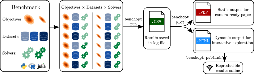
Figure 1: A visual summary of Benchopt. Each Solver is run (in parallel) on each Dataset and each variant of the Objective. Results are exported as a CSV file that is easily shared and can be automatically plotted as interactive html visualizations or PDF figures.

Benchopt provides the tools to structure the optimization for machine learning (Opt-ML) community around standardized benchmarks, and to aggregate individual efforts for reproducibility and results sharing. Benchopt can handle algorithms written in Python, R, Julia or C/C++ via binaries. It offers built-in functionalities to ease the execution of benchmarks: parallel runs, caching, and automatical results archiving. Benchmarks are meant to evolve over time, which is why Benchopt offers a modular structure through which a benchmark can be easily extended with new objective functions, datasets, and solvers by the addition of a single file of code.

The paper is organized as follows. We first detail the design and usage of Benchopt, before presenting results on three canonical problems:

• $\ell_{2}$-regularized logistic regression: a convex and smooth problem which is central to the evaluation of many algorithms in the Opt-ML community, and remains of high relevance for practitioners;

• the Lasso: the prototypical example of non-smooth convex problem in ML;

• training of ResNet18 architecture for image classification: a large scale non-convex deep learning problem central in the field of computer vision.

The reported benchmarks, involving dozens of implementations and datasets, shed light on the current state-of-the-art solvers for each problem, across various settings, highlighting that the best algorithm largely depends on the dataset properties (e.g., size, sparsity), the hyperparameters, as well as hardware. A variety of other benchmarks (e.g., MCP, TV1D, etc.) are also presented in Appendix, with the goal to facilitate contributions from the community.

By the open source and collaborative design of Benchopt (BSD 3-clause license), we aim to open the way towards community-endorsed and peer-reviewed benchmarks that will improve the tracking of progress in optimization for ML.

2 The Benchopt library

The Benchopt library aims to provide a standard toolset and structure to implement benchmarks for optimization in ML, where the problems depend on some input dataset $\mathcal{D}$. The considered problems are of the form

$$\theta^{*}\in\mathop{\mathrm{arg\,min}}_{\theta\in\Theta}f(\theta;\mathcal{D},\Lambda)\enspace,$$ (1)

where $f$ is the objective function, $\Lambda$ are its hyperparameters, and $\Theta$ is the feasible set for $\theta$. The scope of the library is to evaluate optimization methods in their wide sense by considering the sequence $\{\theta^{t}\}_{t}$ produced to approximate $\theta^{*}$. We emphasize than Benchopt does not provide a fixed set of benchmarks, but a framework to create, extend and share benchmarks on any problem of the form (1). To provide a flexible and extendable coding standard, benchmarks are defined as the association of three types of object classes:

.1 benchmark/. .2 objective.py. .2 datasets/. .3 dataset1.py. .3 dataset2.py. .2 solvers/. .3 solver1.py. .3 solver2.py.

Figure 2: Standard benchmark structure

• Objective: It defines the function $f$ to be minimized as well as the hyperparameters $\Lambda$ or the set $\Theta$, and the metrics to track along the iterations (e.g., objective value, gradient norm for smooth problems, or validation loss). Multiple metrics can be registered for each $\theta^{t}$.

• Datasets: The Dataset objects provide the data $\mathcal{D}$ to be passed to the Objective class. They control how data is loaded and preprocessed. Datasets are separated from the Objective, making it easy to add new ones, provided they are coherent with the Objective.

• Solvers: The Solver objects define how to run the algorithm. They are provided with the Objective and Dataset objects and output a sequence $\{\theta^{t}\}_{t}$. This sequence can be obtained using a single run of the method, or with multiple runs in case the method only returns its final iterate.

Each of these objects can have parameters that change their behavior, e.g.,  the regularization parameters for the Objective, the choice of preprocessing for the Datasets, or the step size for the Solvers. By exposing these parameters in the different objects, Benchopt can evaluate their influence on the benchmark results. The Benchopt library defines an application programming interface (API) for each of these concepts and provides a command line interface (CLI) to make them work together. A benchmark is defined as a folder that contains an Objective as well as subfolders containing the Solvers and Datasets. Appendix B presents a concrete example on Ridge regression of how to construct a Benchopt benchmark while additional design design choices of Benchopt are discussed in Appendix C.

For each Dataset and Solver, and for each set of parameters, Benchopt retrieves a sequence $\{\theta^{t}\}_{t}$ and evaluates the metrics defined in the Objective for each $\theta^{t}$. To ensure fair evaluation, the computation of these metrics is done off-line. The metrics are gathered in a CSV file that can be used to display the benchmark results, either locally or as HTML files published on a website that reference the benchmarks run with Benchopt. This workflow is described in Figure 1.

This modular and standardized organization for benchmarks empowers the optimization community by making numerical experiments easily reproducible, shareable, flexible and extendable. The benchmark can be shared as a git repository or a folder containing the different definitions for the Objective, Datasets and Solvers and it can be run with the Benchopt CLI, hence becoming a convenient reference for future comparisons. This ensures fair evaluation of baselines in follow-up experiments, as implementations validated by the community are available. Moreover, benchmarks can be extended easily as one can add a Dataset or a Solver to the comparison by adding a single file. Finally, by supporting multiple metrics – e.g.,  training and testing losses, error on parameter estimates, sparsity of the estimate – the Objective class offers the flexibility to define the concurrent evaluation, which can be extended to track extra metrics on a per benchmark basis, depending on the problem at hand.

As one of the goal of Benchopt is to make benchmarks as simple as possible, it also provides a set of features to make them easy to develop and run. Benchopt is written in Python, but Solvers run with implementations in different languages (e.g., R and Julia, as in Section 4) and frameworks (e.g., PyTorch and TensorFlow, as in Section 5). Moreover, benchmarks can be run in parallel with checkpointing of the results, enabling large scale evaluations on many CPU or GPU nodes. Benchopt also makes it possible to run solvers with many different hyperparameters’ values , allowing to assess their sensitivity on the method performance. Benchmark results are also automatically exported as interactive visualizations, helping with the exploration of the many different settings.

Benchmarks   All presented benchmarks are run on 10 cores of an Intel Xeon Gold 6248 CPUs @ 2.50GHz and NVIDIA V100 GPUs (16GB). The results’ interactive plots and data are available at https://benchopt.github.io/results/preprint_results.html.

3 First example: $\ell_{2}$-regularized logistic regression

Logistic regression is a very popular method for binary classification. From a design matrix $X\in\mathbb{R}^{n\times p}$ with rows $X_{i}$ and a vector of labels $y\in\{-1,1\}^{n}$ with corresponding element $y_{i}$, $\ell_{2}$-regularized logistic regression provides a generalized linear model indexed by $\theta^{*}\in\mathbb{R}^{p}$ to discriminate the classes by solving

$$\theta^{*}=\mathop{\mathrm{arg\,min}}_{\theta\in\mathbb{R}^{p}}\sum_{i=1}^{n}\log\big{(}1+\exp(-y_{i}X_{i}^{\top}\theta)\big{)}+\frac{\lambda}{2}\|\theta\|_{2}^{2}\enspace,$$ (1)

where $\lambda>0$ is the regularization hyperparameter. Thanks to the regularization part, Section 3 is strongly convex with a Lipschitz gradient, and thus its solution can be estimated efficiently using many iterative optimization schemes.

The most classical methods to solve this problem take inspiration from Newton’s method [142]. On the one hand, quasi-Newton methods aim at approximating the Hessian of the cost function with cheap to compute operators. Among these methods, L-BFGS [91] stands out for its small memory footprint, its robustness and fast convergence in a variety of settings. On the other hand, truncated Newton methods [44] try to directly approximate Newton’s direction by using e.g.,  the conjugate gradient method [54] and Hessian-vector products to solve the associated linear system. Yet, these methods suffer when $n$ is large: each iteration requires a pass on the whole dataset.

In this context, methods based on stochastic estimates of the gradient have become standard [21], with Stochastic Gradient Descent (SGD) as a main instance. The core idea is to use cheap and noisy estimates of the gradient [121, 79]. While SGD generally converges either slowly due to decreasing step sizes, or to a neighborhood of the solution for constant step sizes, variance-reduced adaptations such as SAG [126], SAGA [43] and SVRG [75] make it possible to solve the problem more efficiently and are often considered to be state-of-the-art for large scale problems.

Finally, methods based on coordinate descent [14] have also been proposed to solve Section 3. While these methods are usually less popular, they can be efficient in the context of sparse datasets, where only few samples have non-zero values for a given feature, or when accelerated on distributed systems or GPU [46].

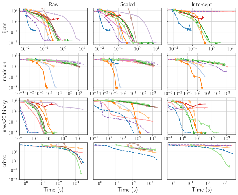
Figure 3: Benchmark for the $\ell_{2}$-regularized logistic regression, on 13 solvers, 4 datasets (rows), and 3 variants of the Objective (columns) with $\lambda=1$. The curves display the suboptimality of the iterates, $f(\theta^{t})-f(\theta^{*})$, as a function of time. The first column corresponds to the objective function detailed in Section 3. In the second column, datasets were preprocessed by normalizing each feature to unit standard deviation. The third column is for an objective function which includes an unregularized intercept.

The code for the benchmark is available at https://github.com/benchopt/benchmark_logreg_l2/. To reflect the diversity of solvers available, we showcase a Benchopt benchmark with 3 datasets, 10 optimization strategies implemented in 5 packages, leveraging GPU hardware when possible. We also consider different scenarios for the objective function: (i) scaling (or not) the features, a recommended data preprocessing step, crucial in practice to have comparable regularization strength on all variables; (ii) fitting (or not) an unregularized intercept term, important in practice and making optimization harder when omitted from the regularization term [81]; (iii) working (or not) with sparse features, which prevent explicit centering during preprocessing to keep memory usage limited. Details on packages, datasets and additional scenarios are available in Appendix D.

Results   Figure D.1 presents the results of the benchmarks, in terms of suboptimality of the iterates, $f(\theta^{t})-f(\theta^{*})$, for three datasets and three scenarios. Here, because the problem is convex, $\theta^{*}$ is approximated by the best iterate across all runs (see Section C.1). Overall, the benchmark shows the benefit of using GPU solvers (cuML and snapML), even for small scale tasks such as ijcnn1. Note that these two accelerated solvers converge to a higher suboptimality level compared to other solvers, due to operating with 32-bit float precision. Another observation is that data scaling can drastically change the picture. In the case of madelon, most solvers have a hard time converging for the scaled data. For the solvers that converge, we note that the convergence time is one order of magnitude smaller with the scaled dataset compared to the raw one. This stems from the fact that in this case, the scaling improves the conditioning of the dataset. For news20.binary, the stochastic solvers such as SAG and SAGA have degraded performances on scaled data. Here, the scaling makes the problem harder.

On CPU, quasi-Newton solvers are often the most efficient ones, and provide a reasonable choice in most situations. For large scale news20.binary, stochastic solvers such as SAG, SAGA or SVRG –that are often considered as state of the art for such problem– have worst performances for the presented datasets. While this dataset is often used as a test bed for benchmarking new stochastic solvers, we fail to see an improvement over non-stochastic ones for this experimental setup. In contrast, the last row in Figure D.1 displays an experiment with the larger scale criteo dataset, which demonstrates a regime where variance-reduced stochastic gradient methods outperform quasi-Newton methods. For future benchmarking of stochastic solvers, we therefore recommend using such a large dataset.

Finally, the third column in Figure D.1 illustrates a classical problem when benchmarking different solvers: their specific (and incompatible) definition and resolution of the corresponding optimization problem. Here, the objective function is modified to account for an intercept (bias) in the linear model. In most situations, this intercept is not regularized when it is fitted. However, snapML and liblinear solvers do regularize it, leading to incomparable losses.

4 Second example: The Lasso

The Lasso, [134, 33], is an archetype of non-smooth ML problems, whose impact on ML, statistics and signal processing in the last three decades has been considerable [29, 67]. It consists of solving

$$\theta^{*}\in\mathop{\mathrm{arg\,min}}_{\theta\in\mathbb{R}^{p}}\tfrac{1}{2}\left\|y-X\theta\right\|^{2}+\lambda\left\|\theta\right\|_{1}\enspace,$$ (1)

where $X\in\mathbb{R}^{n\times p}$ is a design matrix containing $p$ features as columns, $y\in\mathbb{R}^{n}$ is the target vector, and $\lambda>0$ is a regularization hyperparameter. The Lasso estimator was popularized for variable selection: when $\lambda$ is high enough, many entries in $\theta^{*}$ are exactly equal to 0. This leads to more interpretable models and reduces overfitting compared to the least-squares estimator.

Solvers for Section 4 have evolved since its introduction by [134]. After generic quadratic program solvers, new dedicated solvers were proposed based on iterative reweighted least-squares (IRLS) [62], followed by LARS [47], a homotopy method computing the full Lasso path. The LARS solver helped popularize the Lasso, yet the algorithm suffers from stability issues and can be very slow for worst case situations [96]. General purpose solvers became popular for Lasso-type problems with the introduction of the iterative soft thresholding algorithm (ISTA, [42]), an instance of forward-backward splitting [37]. These algorithms became standard in signal and image processing, especially when accelerated (FISTA, [8]).

In parallel, proximal coordinate descent has proven particularly relevant for the Lasso in statistics. Early theoretical results were proved by [137, 125], before it became the standard solver of the widely distributed packages glmnet in R and scikit-learn in Python. For further improvements, some solvers exploit the sparsity of $\theta^{*}$, trying to identify its support to reduce the problem size. Best performing variants of this scheme are screening rules (e.g.,  [48, 20, 104]) and working/active sets (e.g.,  [76, 98]), including strong rules [133].

While reviews of Lasso solvers have already been performed [3, Sec. 8.1], they are limited to certain implementation and design choices, but also naturally lack comparisons with more recent solvers and modern hardware, hence drawing biased conclusions.

The code for the benchmark is available at https://github.com/benchopt/benchmark_lasso/. Results obtained on 4 datasets, with 9 standard packages and some custom reimplementations, possibly leveraging GPU hardware, and 17 different solvers written in Python/numba/Cython, R, Julia or C++ (Table E.1) are presented in Figure 4. All solvers use efficient numerical implementations, possibly leveraging calls to BLAS, precompiled code in Cython or just-in-time compilation with numba.

The different parameters influencing the setup are

• the regularization strength $\lambda$, controlling the sparsity of the solution, parameterized as a fraction of $\lambda_{\max}=\left\|X^{\top}y\right\|_{\infty}$ (the minimal hyperparameter such that $\theta^{*}=0$),

• the dataset dimensions: MEG has small $n$ and medium $p$; rcv1.binary has medium $n$ and $p$; news20.binary has medium $n$ and very large $p$ while MillionSong has very large $n$ and small $p$ (Table E.2).

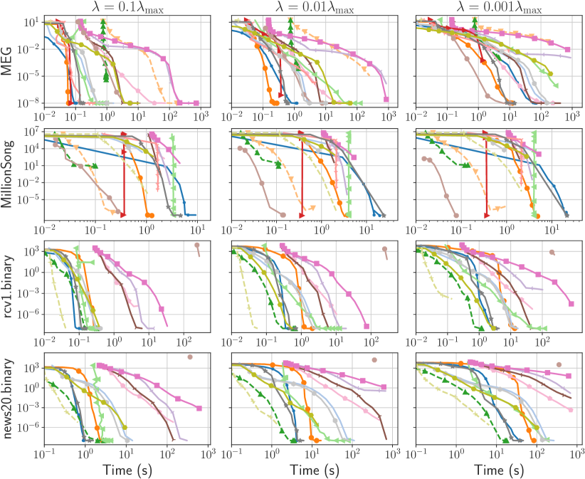
Figure 4: Benchmark for the Lasso, on 17 solvers, 4 datasets (rows), and 3 variants of the Objective (columns) with decreasing regularization $\lambda$. The curves display the suboptimality of the objective function, $f(\theta^{t})-f(\theta^{*})$, as a function of time.

Results   Figure 4 presents the result of the benchmark on the Lasso, in terms of objective suboptimality $f(\theta^{t})-f(\theta^{*})$ as a function of time.

Similarly to Section 3, the GPU solvers obtain good performances in most settings, but their advantage is less clear. A consistent finding across all settings is that coordinate descent-based methods outperform full gradient ones (ISTA and FISTA, even restarted), and are improved by the use of working set strategies (blitz, celer, skglm, glmnet). This observation is even more pronounced when the regularization parameter is large, as the solution is sparser.

When observing the influence of the dataset dimensions, we observe 3 regimes. When $n$ is small (MEG), the support of the solution is small and coordinate descent, LARS and noncvx-pro perform the best. When $n$ is much larger than $p$ (MillionSong), noncvx-pro clearly outperforms other solvers, and working set methods prove useless. Finally, when $n$ and $p$ are large (rcv1.binary, news20.binary), CD and working sets vastly outperforms the rest while noncvx-pro fails, as it requires solving a linear system of size $\min(n,p)$. We note that this setting was not tested in the original experiment of [112], which highlights the need for extensive, standard experimental setups.

When the support of the solution is small (either small $\lambda$, either small $n$ since the Lasso solution has at most $n$ nonzero coefficients), LARS is a competitive algorithm. We expect this to degrade when $n$ increases, but as the LARS solver in scikit-learn does not support sparse design matrices we could not include it for news20.binary and rcv1.binary.

This benchmark is the first to evaluate solvers across languages, showing the competitive behavior of lasso.jl and glmnet compared to Python solvers. Both solvers have a large initialization time, and then converge very fast. To ensure that the benchmark is fair, even though the Benchopt library is implemented in Python, we made sure to ignore conversion overhead, as well as just-in-time compilation cost. We also checked the timing’s consistency with native calls to the libraries.

Since the Lasso is massively used for it feature selection properties, the speed at which the solvers identify the support of the solution is also an important performance measure. Monitoring this with Benchopt is straightforward, and a figure reporting this benchmark is in Appendix E.

5 Third example: How standard is a benchmark on ResNet18?

As early successes of deep learning have been focused on computer vision tasks [86], image classification has become a de facto standard to validate novel methods in the field. Among the different network architectures, ResNets [69] are extensively used in the community as they provide strong and versatile baselines [143, 132, 45, 28, 92]. While many papers present results with such model on classical datasets, with sometimes extensive ablation studies [70, 141, 9, 127], the lack of standardized codebase and missing implementation details makes it hard to replicate their results.

The code for the benchmark is available at https://github.com/benchopt/benchmark_resnet_classif/. We provide a cross-dataset –SVHN, [106]; MNIST, [88] and CIFAR-10, [85]– and cross-framework –TensorFlow/Keras, [1, 35]; PyTorch, [107]– evaluation of the training strategies for image classification with ResNet18 (see Appendix F for details on architecture and datasets). We train the network by minimizing the cross entropy loss relatively to the weights $\theta$ of the model. Contrary to logistic regression and the Lasso, this problem is non-convex due to the non-linearity of the model $f_{\theta}$. Another notable difference is that we report the evolution of the test error rather than the training loss.

Because we chose to monitor the test loss, the Solvers are defined as the combination of an optimization algorithm, its hyperparameters, the learning rate (LR) and weight decay schedules, and the data augmentation strategy. This is in contrast to a case where we would monitor the train loss, and therefore make the LR and weight decay schedules, as well as the data augmentation policy, part of the objective. We focus on 2 standard methods: stochastic gradient descent (SGD) with momentum and Adam [80], as well as a more recently published one: Lookahead [145]. The LR schedules are chosen among fixed LR, step LR, and cosine annealing [93]. We also consider decoupled weight decay for Adam [94], and coupled weight decay (i.e., $\ell_{2}$-regularization) for SGD. Regarding data augmentation, we use random cropping for all datasets and add horizontal flipping only for CIFAR-10, as the digits datasets do not exhibit a mirror symmetry. We detail the remaining hyperparameters in Table F.2, and discuss their selection as well as their sensitivity in Appendix F.

Aligning cross-framework implementations   Due to some design choices, components with the same name in the different frameworks do not have the same behavior. For instance, when it comes to applying weight decay, PyTorch’s SGD uses coupled weight decay, while in TensorFlow/Keras weight decay always refers to decoupled weight decay. These two methods lead to significantly different performance and it is not straightforward to apply coupled weight decay in a post-hoc manner in TensorFlow/Keras (see further details in Section F.3). We conducted an extensive effort to align the networks implementation in different frameworks using unit testing to make the conclusions of our benchmarks independent of the chosen framework. We found additional significant differences (reported in Table F.3) in the initialization, the batch normalization, the convolutional layers and the weight decay scaling.

Results

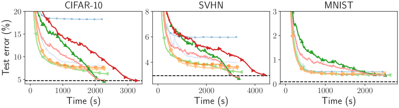
Figure 5: ResNet18 image classification benchmark with PyTorch Solvers. The best SGD configuration features data augmentation, momentum, cosine learning rate schedule and weight decay. In dashed black is the state of the art for the corresponding datasets with a ResNet18 measured by [145] for CIFAR-10, by [147] for SVHN with a PreAct ResNet18, by PapersWithCode for MNIST with all networks considered. Off-the-shelf ResNet implementations in TensorFlow/Keras do not support images smaller than $32\times 32$ and is hence not shown for MNIST.Curves are exponentially smoothed.

The results of the benchmark are reported in Figure 5. Each graph reports the test error relative to time, with an ablation study on the solvers parameters. Note that we only report selected settings for clarity but that we run every possible combinations..

Firstly, reaching the state of the art for a vanilla ResNet18 is not straightforward. On the popular website Papers with code it has been so far underestimated. It can achieve 4.45% and 2.65% test error rates on CIFAR-10 and SVHN respectively (compared to 4.73% and 2.95% – for a PreAct ResNet18 – before that). Our ablation study shows that a variety of techniques is required to reach it. The most significant one is an appropriate data augmentation strategy, which lowers the error rate on CIFAR-10 from about 18% to about 8%. The second most important one is weight decay, but it has to be used in combination with a proper LR schedule, as well as momentum. While these techniques are not novel, they are regularly overlooked in baselines, resulting in underestimation of their performance level.

This reproducible benchmark not only allows a researcher to get a clear understanding of how to achieve the best performances for this model and datasets, but also provides a way to reproduce and extend these performances. In particular, we also include in this benchmark the original implementation of Lookahead [145]. We confirm that it slightly accelerates the convergence of the Best SGD, even with a cosine LR schedule – a setting that had not been studied in the original paper.

Our benchmark also evaluates the relative computational performances of the different frameworks. We observe that PyTorch-Lightning is significantly slower than the other frameworks we tested, in large part due to their callbacks API. We also notice that our TensorFlow/Keras implementation is significantly slower ($\approx$ 28%) than the PyTorch ones, despite following the best practices and our profiling efforts. Note that we do not imply that TensorFlow is intrinsically slower than PyTorch, but a community effort is needed to ensure that the benchmark performances are framework-agnostic.

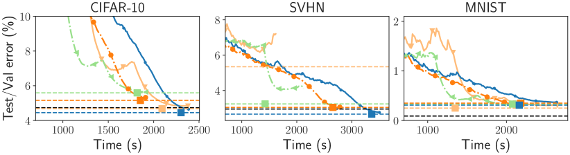
Figure 6: ResNet18 image classification benchmark with a validation split. In dashed black is the state of the art (see caption of Figure 5 for more details). In addition, we show in colored horizontal dashed lines, the test results for early stopping on the validation and on the test set for the different solvers, the square mark indicating the moment this stopping would happen. The curves for the train-val splits show the exponentially smoothed median results for five different random seeds.

A recurrent criticism of such benchmarks is that only the best test error is reported. In Figure 6, we measure the effect of using a train-validation-test split, by keeping a fraction of the training set as a validation set. The splits we use are detailed in Table F.1. Our finding is that the results of the ablation study do not change significantly when using such procedure, even though their validity is reinforced by the use of multiple trainings. Yet, a possible limitation of our findings is that some of the hyperparameters we used for our study, coming from the PyTorch-CIFAR GitHub repository, may have been tuned while looking at the test set.

6 Conclusion and future work

We have introduced Benchopt, a library that makes it easy to collaboratively develop fair and extensive benchmarks of optimization algorithms, which can then be seamlessly published, reproduced, and extended. In the future, we plan on supporting the creation of new benchmarks, that could become the standards the community builds on. This work is part of a wider effort to improve reproducibility of machine learning results. It aims to contribute to raising the standard of numerical validation for optimization, which is pervasive in the statistics and ML community as well as for the experimental sciences that rely more and more on these tools for research.

7 Acknowledgements

It can not be stressed enough how much the Benchopt library relies on contributions from the community and in particular the Python open source ecosystem. In particular, it could not exist without the libraries mentioned in Appendix A.

This work was granted access to the HPC resources of IDRIS under the allocation 2022-AD011011172R2 and 2022-AD011013570 made by GENCI, which was used to run all the benchmarks. MM also gratefully acknowledges the support of the Centre Blaise Pascal’s IT test platform at ENS de Lyon (Lyon, France) for Machine Learning facilities. The platform operates the SIDUS solution [116].

TL, CFD and JS contributions were supported by the Chaire IA CaMeLOt (ANR-20-CHIA-0001-01). AG, EL and TM contributions were supported by the Chaire IA ANR BrAIN (ANR-20-CHIA-0016). BMa contributions were supported by a grant from Digiteo France. MD contributions were supported by a public grant overseen by the French National Research Agency (ANR) through the program UDOPIA, project funded by the ANR-20-THIA-0013-01 and DATAIA convergence institute (ANR-17-CONV-0003). BN work was supported by the Télécom Paris’s Chaire DSAIDIS (Data Science & Artificial Intelligence for Digitalized Industry Services). BMo contributions were supported by a grant from the Labex MILYON.

bergstra2012random

Checklist

1. For all authors…

   1. Do the main claims made in the abstract and introduction accurately reflect the paper’s contributions and scope? [Yes]

   2. Did you describe the limitations of your work? [Yes]

   3. Did you discuss any potential negative societal impacts of your work? [Yes]

   4. Have you read the ethics review guidelines and ensured that your paper conforms to them? [Yes]

2. If you are including theoretical results…

   1. Did you state the full set of assumptions of all theoretical results? [N/A]

   2. Did you include complete proofs of all theoretical results? [N/A]

3. If you ran experiments…

   1. Did you include the code, data, and instructions needed to reproduce the main experimental results (either in the supplemental material or as a URL)? [Yes]

   2. Did you specify all the training details (e.g., data splits, hyperparameters, how they were chosen)? [Yes] These are specified in Appendix, on a per-benchmark basis.

   3. Did you report error bars (e.g., with respect to the random seed after running experiments multiple times)? [No] Error bars are not reported for clarity, but Benchopt allows this in particular in html versions of the plots that can be found in https://benchopt.github.io/results/preprint_results.html.

   4. Did you include the total amount of compute and the type of resources used (e.g., type of GPUs, internal cluster, or cloud provider)? [Yes]

4. If you are using existing assets (e.g., code, data, models) or curating/releasing new assets…

   1. If your work uses existing assets, did you cite the creators? [Yes]

   2. Did you mention the license of the assets? [Yes] In the introduction.

   3. Did you include any new assets either in the supplemental material or as a URL? [Yes]

   4. Did you discuss whether and how consent was obtained from people whose data you’re using/curating? [N/A]

   5. Did you discuss whether the data you are using/curating contains personally identifiable information or offensive content? [N/A]

5. If you used crowdsourcing or conducted research with human subjects…

   1. Did you include the full text of instructions given to participants and screenshots, if applicable? [N/A]

   2. Did you describe any potential participant risks, with links to Institutional Review Board (IRB) approvals, if applicable? [N/A]

   3. Did you include the estimated hourly wage paid to participants and the total amount spent on participant compensation? [N/A]

Appendix A Software ecosystem acknowledgement

The command line interface and API use the click, pyyaml and psutil [122] libraries.

Numerical computations involve numpy [66] and scipy [139]. For cross-language processing, we used rpy2 for calling R [117] libraries and PyJulia for interfacing with Julia [15]. The benchmark runs extensively use joblib, loky [102] and submitit for parallelization.

The results are stored and processed for visualizations using pandas [101], matplotlib [71] for static rendering, mako and plotly [73] for interactive webpages. The participative results website relies partially on pygithub.

Our documentation is generated by multiple sphinx-based [25] libraries (sphinx-bootstrap-theme, sphinx-click, sphinx-gallery [103] and sphinx-prompt), and also the numpydoc and pillow [36] libraries.

Appendix B A complete Benchmark example: Objective, Dataset and Solver classes for Ridge regression

Here, we provide code examples for a simple benchmark on Ridge regression. The Ridge regression – also called $\ell_{2}$-regularized least-squares or Tikhonov regression – is a popular method to solve least-square problems in the presence of noisy observations or correlated features. The problem reads:

$$\min_{\theta}\frac{1}{2}\|y-X\theta\|_{2}^{2}+\frac{\lambda}{2}\|\theta\|_{2}^{2}\enspace,$$ (1)

where $X\in\mathbb{R}^{n\times p}$ is a design matrix, $y\in\mathbb{R}^{n}$ is the target vector and $\lambda$ is the regularization parameter. This problem is strongly convex and many methods can be used to solve it. Direct computation of the close form solution $\theta^{*}=(X^{\top}X+\lambda Id)^{-1}X^{\top}y$ can be obtained using matrix factorization methods such as Cholesky decomposition or the SVD [114] or iterative linear solver such as Conjugate-Gradient [91]. One can also resort on first order methods such as gradient descent, coordinate descent (known as the Gauss-Seidel method in this context), or their stochastic variant.

The code for the benchmark is available at https://github.com/benchopt/benchmark_ridge/. The following code snippets are provided in the documentation as a template for new benchmarks.

B.1 Objective class

The Objective class is the central part of the benchmark, defining the objective function. This class allows us to monitor the quantities of interest along the iterations of the solvers, amongst which the objective function value. An Objective class should define 3 methods:

• set_data(**data): it allows specifying the nature of the data used in the benchmark. The data is passed as a dictionary of Python variables, so no constraint is enforced to what can be passed here.

• compute(theta): it allows evaluating the objective function for a given value of the iterate, here called $\theta$. This method should take only one parameter, the output returned by the Solver. All other parameters should be stored in the class with the set_data method. The compute function should return a float (understood as the objective value) or a dictionary. If a dictionary is returned it should contain a key called value (the objective value) and all other keys should correspond to float values allowing tracking more than one quantity of interest (e.g. train and test errors).

• to_dict(): a method that returns a dictionary to be passed to the set_objective() method of a Solver.

An Objective class needs to inherit from a base class, benchopt.BaseObjective. Below is the implementation of the Ridge regression Objective class.

from benchopt import BaseObjective

class Objective(BaseObjective): name = "Ridge regression" parameters = "reg": [0.1, 1, 10]

def __init__(self, reg=1): self.reg = reg

def set_data(self, X, y): self.X, self.y = X, y

def compute(self, theta): res = self.y - self.X @ theta return .5 * res @ res + 0.5 * self.reg * theta @ theta

def to_dict(self): return dict(X=self.X, y=self.y, reg=self.reg)

B.2 Dataset class

A Dataset class defines data to be passed to the Objective. More specifically, a Dataset class should implement one method:

• get_data(): A method outputting a dictionary that can be passed as keyword arguments **data to the set_data method of the Objective.

A Dataset class also needs to inherit from a base class, benchopt.BaseDataset.

If a Dataset requires some packages to function, Benchopt allows listing some requirements. The necessary packages should be available via conda or pip.

Below is an example of a Dataset definition using the libsvmdata library, which exposes datasets from libsvm, such as leukemia, bodyfat and gisette – described in Table B.1.

from benchopt import BaseDataset from benchopt import safe_import_context

# This context allow to manipulate the Dataset object even if # libsvmdata is not installed. It is used in ‘benchopt install‘. with safe_import_context() as import_ctx: from libsvmdata import fetch_libsvm

class Dataset(BaseDataset): name = "libsvm" install_cmd = "conda" requirements = ["libsvmdata"] parameters = "dataset": ["bodyfat", "leukemia", "gisette"]

def __init__(self, dataset="bodyfat"): self.dataset = dataset

def get_data(self): X, y = fetch_libsvm(self.dataset) return dict(X=self.X, y=self.y)

B.3 Solver class

A Solver class must define three methods:

• set_objective(**objective_dict): This method will be called with the dictionary objective_dict returned by the method to_dict from the Objective. The goal of this method is to provide all necessary information to the Solver so it can optimize the objective function.

• run(stop_value): This method takes only one parameter that controls the stopping condition of the Solver. Typically this is either a number of iterations n_iter or a tolerance parameter tol. Alternatively, a callback function that will be called at each iteration can be passed. The callback should return False once the computation should stop. The parameter stop_value is controlled by the stopping_strategy, see below for details.

• get_result(): This method returns a variable that can be passed to the compute method from the Objective. This is the output of the Solver.

If a Python Solver requires some packages such as scikit-learn, Benchopt allows listing some requirements. The necessary packages must be available via conda or pip.

Below is a simple Solver example using scikit-learn implementation of Ridge regression with different optimization algorithms.

from benchopt import BaseSolver from benchopt import safe_import_context

# This context allow to manipulate the Solver object even if # scikit-learn is not installed. It is used in ‘benchopt install‘. with safe_import_context() as import_ctx: from sklearn.linear_model import Ridge

class Solver(BaseSolver): name = "scikit-learn" install_cmd = "conda" requirements = ["scikit-learn"] parameters = "alg": ["svd", "cholesky", "lsqr", "sparse_cg", "saga"],

def __init__(self, alg="svd"): self.alg = alg

def set_objective(self, X, y, reg=1): self.X, self.y = X, y self.clf = Ridge( fit_intercept=False, alpha=reg, solver=self.alg, tol=1e-10 )

def run(self, n_iter): self.clf.max_iter = n_iter + 1 self.clf.fit(self.X, self.y)

def get_result(self): return self.clf.coef_

B.4 Results from the benchmark

Descriptions of datasets   Table B.1 describes the datasets used in this benchmarks.

Table B.1: List of the datasets used in Ridge regression in Appendix B

Datasets	References	Samples ($\mathbf{n}$)	Features ($\mathbf{p}$)
leukemia	[59]	$38$	$7129$
bodyfat	[63]	$252$	$8$
gisette	[63]	$6000$	$5000$

We also run the solvers on the simulated data described bellow.

Generation process for simulated dataset   We generate a linear regression scenario with decaying correlation for the design matrix, i.e., the ground-truth covariance matrix is a Toeplitz matrix, with each element $\Sigma_{ij}=\rho^{|i-j|}$. As a consequence, the generated features have 0 mean, a variance of 1, and the correlation structure as:

$$\mathbb{E}[X_{i}]=0~{},\quad\mathbb{E}[X_{i}^{2}]=1\quad\text{and}\quad\mathbb{E}[X_{i}X_{j}]=\rho^{|i-j|}\ .$$ (2)

Our simulation scheme also includes the parameter $\texttt{density}=0.2$ that controls the proportion of non-zero elements in $\theta^{*}$. The target vector is generated according to linear relationship with Gaussian noise:

$$y=X\theta^{*}+\varepsilon\ ,$$

such that the signal-to-noise ratio is $\texttt{snr}=\frac{\|X\theta^{*}\|_{2}}{\|\varepsilon\|_{2}}$.

We use a signal-to-noise ratio $\texttt{snr}=3$, a correlation $\rho$ of $0$ or $0.6$ with $n=500$ samples and $p=1000$ features.

Description of the solvers   Table B.2 describes the different solvers compared in this benchmark.

Table B.2: List of solvers used in the Ridge benchmark in Appendix B

Solver	References	Description	Language
GD	[23]	Gradient Descent	Python
Accelerated GD	[105]	Gradient Descent + acceleration	Python
scikit-learn[svd]	[109]	SVD (Singular Value Decomposition)	Python (Cython)
scikit-learn[cholesky]	[109]	Cholesky decomposition	Python (Cython)
scikit-learn[lsqr]	[109]	regularized least-squares	Python (Cython)
scikit-learn[saga]	[109]	SAGA (Varianced reduced stochastic method)	Python (Cython)
scikit-learn[cg]	[109]	Conjugate Gradient	Python (Cython)
CD	[14]	Cyclic Coordinate Descent	Python (Numba)
lightning[cd]	[17]	Cyclic Coordinate Descent	Python (Cython)
snapML[cpu]	[46]	CD	Python, C++
snapML[gpu]	[46]	CD + GPU	Python, C++

Results   Figure B.1 presents the performance of the different methods for different values of the regularization parameter in the benchmark. The algorithms based on the direct computation of the closed-form solution outperform iterative ones in a majority of presented datasets. Among closed-form algorithms, the Cholesky solver converges faster.

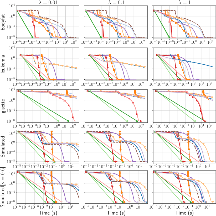
Figure B.1: Benchmark for the Ridge regression, on 10 solvers, 5 datasets (rows), and 3 variants of the Objective (columns) each with a different regularization value $\lambda\in\{0.01,0.1,1\}$. The curves display the suboptimality of the iterates, $f(\theta^{t})-f(\theta^{*})$, as a function of time.

Appendix C Design choices

Benchopt has made some design choices, while trying as much as possible to leave users free of customizing the behavior on each benchmark. We detail the most important ones in this section.

C.1 Estimating $\theta^{*}$ for convex problems

When the problem is convex, many solvers are guaranteed to converge to a global minimizer $\theta^{*}$ of the objective function $f$. To estimate $\theta^{*}$ and $f(\theta^{*})$, Benchopt approximates $\theta^{*}$ by the iterate achieving the lowest objective_value among all solvers for a given Dataset and Objective. This means that the sub-optimality plot proposed by Benchopt are only valid if at least one solver has converged to the optimal solution. Else, the curves are a lower bound estimate of the sub-optimality. In practice, for most considered convex problems, running the Solver for long enough ensures that $f(\theta^{*})$ is correctly estimated.

C.2 Stopping solvers

Benchopt offers many ways to stop running a solver. The most common is to stop the solver when the objective value does not decrease significantly between iterations. For some convex problems, we also propose to track the duality gap (which upper bounds the suboptimality), as is done for the Lasso. For non convex problems, criteria such as gradient norm or violation of first order conditions can be used, as users do in practice. These criteria can easily be customized.

C.3 Wall-clock time versus number of iterations

Measuring time or iteration are two alternatives that make sense in their respective contexts. Practitioners mostly care about the time it takes to solve their problem, while researchers in mathematical optimization may want to abstract away the implementation and hardware details and only consider iteration. The benchmarks we have presented showcase efficient implementations and are also interested in hardware and implementation differences (e.g. CPU vs GPU solvers for LABEL:sec:logreg,sec:lasso, torch versus tensorflow for Section F.4), hence our focus on time. However, Benchopt does not impose a choice between the two measures: it is perfectly possible to create plots as a function of the number of iterations as evidenced for example in LABEL:app:sec:lasso_iteration.

Appendix D $\ell_{2}$-regularized logistic regression

D.1 List of solvers and datasets used in the benchmark in Section 3

Table D.1 and Table D.2 respectively present the Solvers and Datasets used in this benchmark.

Table D.1: List of solvers used in the $\ell_{2}$-regularized logistic regression benchmark in Section 3

Solver	References	Description	Language
lightning[sag]	[17]	SAG	Python (Cython)
lightning[saga]	[17]	SAGA	Python (Cython)
lightning[cd]	[17]	Cyclic Coordinate Descent	Python (Cython)
Tick[svrg]	[4]	Stochastic Variance Reduced Gradient	Python, C++
scikit-learn[sgd]	[109]	Stochastic Gradient Descent	Python (Cython)
scikit-learn[sag]	[109]	SAG	Python (Cython)
scikit-learn[saga]	[109]	SAGA	Python (Cython)
scikit-learn[liblinear]	[109], [52]	Truncated Newton Conjugate-Gradient	Python (Cython)
scikit-learn[lbfgs]	[109], [139]	L-BFGS (Quasi-Newton Method)	Python (Cython)
scikit-learn[newton-cg]	[109], [139]	Truncated Newton Conjugate-Gradient	Python (Cython)
snapml[cpu]	[46]	CD	Python, C++
snapml[gpu]	[46]	CD + GPU	Python, C++
cuML[gpu]	[120]	L-BFGS + GPU	Python, C++

Table D.2: List of the datasets used in $\ell_{2}$-regularized logistic regression in Section 3

Datasets	References	Samples ($\mathbf{n}$)	Features ($\mathbf{p}$)	Density
ijcnn1	[115]	$49\,990$	$22$	$0.045$
madelon	[63]	$2000$	$500$	$0.0020$
news20.binary	[78]	$19\,996$	$1\,355\,191$	$0.000\,34$
criteo	[41]	$45\,840\,617$	$1\,000\,000$	$0.000\,039$

D.2 Results

Figure D.1 presents the performance results for the different solvers on the different datasets using various regularization parameter values, on unscaled raw data. We observe that when the regularization parameter $\lambda$ increases, the problem tends to become easier and faster to solve for most methods. Also, the relative order of the method does not change significantly for the considered range of regularization.

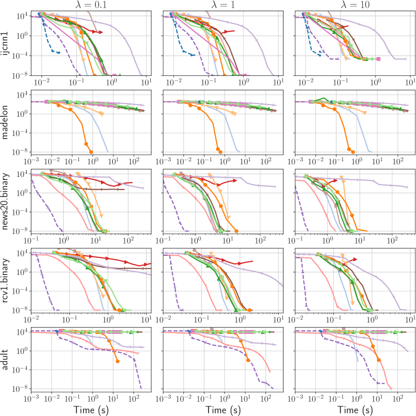
Figure D.1: Additional benchmark for the $\ell_{2}$-regularized logistic regression on variants of the Objective (columns) with fit_intercept=False. The curves display the suboptimality of the iterates, $f(\theta^{t})-f(\theta^{*})$, as a function of time. The columns correspond to the objective detailed in Section 3 with different value of $\lambda$: (first) $\lambda=0.1$, (second) $\lambda=1$ and (third) $\lambda=10$.

Appendix E Lasso

E.1 List of solvers and datasets used in the Lasso benchmark in Section 4

Table E.1 and Table E.2 respectively present the Solvers and Datasets used in this benchmark.

Table E.1: List of solvers used in the Lasso benchmark in Section 4

Solver	References	Description	Language
blitz	[76]	CD + working set	Python, C++
coordinate descent	[56]	(Cyclic) Minimization along coordinates	Python (Numba)
celer	[98]	CD + working set + dual extrapolation	Python (Cython)
cuML[cd]	[120]	(Cyclic) Minimization along coordinates	Python, C++
cuML[qn]	[120]	Orthant-Wise Limited Memory Quasi-Newton (OWL-QN)	Python, C++
FISTA	[8]	ISTA + acceleration	Python
glmnet	[56]	CD + working set + strong rules	R, C++
ISTA	[42]	ISTA (Proximal GD)	Python
LARS	[47]	Least-Angle Regression algorithm (LARS)	Python (Cython)
FISTA[adaptive-1]	[90, Algo 4 ], [53]	FISTA + adaptive restart	Python
FISTA[greedy]	[90, Algo 5 ], [53]	FISTA + greedy restart	Python
noncvx-pro	[112]	Bilevel optim + L-BFGS	Python (Cython)
skglm	[13]	CD + working set + primal extrapolation	Python (Numba)
scikit-learn	[109]	CD	Python (Cython)
snapML[gpu]	[46]	CD + GPU	Python, C++
snapML[cpu]	[46]	CD	Python, C++
lasso.jl	[84]	CD	Julia

Table E.2: List of datasets used in the Lasso benchmark in Section 4

Dataset	References	Samples ($\mathbf{n}$)	Features ($\mathbf{p}$)	Density
MEG	[61]	$305$	$7498$	$1.0$
news20	[78]	$19\,996$	$1\,355\,191$	$0.000\,34$
rcv1	[89]	$20\,242$	$47\,236$	$0.0036$
MillionSong	[12]	$463\,715$	$90$	$1$

E.2 Support identification speed benchmark

Since the Lasso is massively used for its feature selection properties, the speed at which the solvers identify the support of the solution is also an important performance measure. To evaluate the behavior of solvers in this task, it is sufficient to add a single new variable in the Objective, namely the $\ell_{0}$ pseudonorm of the iterate, allowing to produce Figure E.1 in addition to Figure 4.

Figure E.1: Additional benchmark for the Lasso on variants of the Objective (columns). The curves display the fraction of non-zero coefficients in iterates $\theta_{t}$ ($\|\theta_{t}\|_{0}/p$), as a function of time.

E.3 Convergence in terms of iteration

LABEL:app:sec:lasso_iteration

While practitioners are mainly concerned with the time it takes to solve their optimization problem, one may also be interested in the convergence as a function of the number of iterations. This is particularly relevant to compare theoretical convergence rates with experiments. Benchopt natively supports such functionality. Yet, this makes sense only if one iteration of each algorithm costs the same. Figure E.2 presents such a case on the leukemia dataset, using algorithms for which one iteration costs $n\times p$. One can observe that cyclic coordinate descent as implemented in Cython in scikit-learn or in Numba lead to identical results, while they outperform proximal gradient methods.

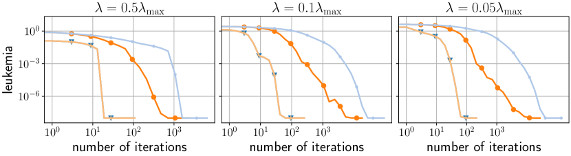
Figure E.2: Convergence speed with respect to the number of iterations for some solvers of the Lasso benchmark on the leukemia dataset.

Appendix F ResNet18

F.1 Description of the benchmark

Setting up the benchmark   The three currently supported frameworks are TensorFlow/Keras [1, 35], PyTorch [107] and PyTorch Lightning [50]. We report here results for TensorFlow/Keras and PyTorch. To guarantee that the model behaves consistently across the different considered frameworks, we implemented several consistency unit tests. We followed the best practice of each framework to make sure to achieve the optimal computational efficiency. In particular, we tried as much as possible to use official code from the frameworks, and not third-party code. We also optimized and profiled the data pipelines to make sure that our training was not IO-bound. Our benchmarks were run using TensorFlow version 2.8 and PyTorch version 1.10.

Descriptions of the datasets

Table F.1: Description of the datasets used in the ResNet18 image classification benchmark

Dataset	Content	References	Classes	Train Size	Val. Size	Test Size	Image Size	RGB
CIFAR-10	natural images	[85]	10	$40$k	$10$k	$10$k	32	✓
SVHN	digits in natural images	[106]	10	$58.6$k	$14.6$k	$26$k	32	✓
MNIST	handwritten digits	[88]	10	$50$k	$10$k	$10$k	28	✗

In Table F.1, we present some characteristics of the different datasets used for the ResNet18 benchmark. In particular, we specify the size of each splits when using the train-validation-test split strategy. The test split is always fixed, and is the official one.

While the datasets are downloaded and preprocessed using the official implementations of the frameworks, we made sure to test that they matched using a unit test.

ResNet   The ResNet18 is the smallest variant of the architecture introduced by [69]. It consists in 3 stages:

1. A feature extension convolution that goes from 3 channels (RGB, or a repeated grayscale channel in the MNIST case) to 64, followed by a batch normalization and a ReLU.

2. A series of residual blocks. Residual blocks are grouped by scale, and each individual group starts with a strided convolution to reduce the image scale (except the first one). As the scale increases, so does the number of features (64, 128, 256, 512). In the ResNet18 case, each scale group has two individual residual blocks and there are four scales. A residual block is comprised of three convolution operations, all followed by a batch normalization layer, and the first two also followed by a ReLU. The input is then added to the output of the third batch normalization layer before being fed to a ReLU.

3. A classification head that performs global average pooling, before applying a fully connected (i.e. dense) layer to obtain logits.

Training’s hyperparameters

Table F.2: Hyperparameters used for each solver. If a hyperparameter’s value is not specified in the table, it was set as the default of the implementation (checked to be consistent across frameworks).

Hyperparameter	SGD	Adam
Learning Rate	0.1	0.001
Momentum	0.9	N/A
Weight Decay	$5\times 10^{-4}$	0.02
Batch Size	128	128

In Table F.2, we specify the hyperparameters we used for the benchmark. For the SGD, the values were taken from the pytorch-cifar GitHub repository, while for Adam we took the most relevant ones from the work of [141].

F.2 Hyperparameter sensitivity

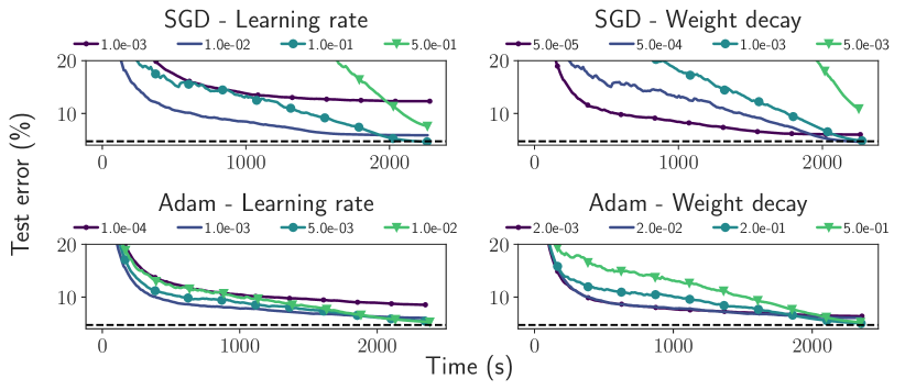
Figure F.1: ResNet18 image classification benchmark on CIFAR-10 for different values of learning rate and weight decay for SGD and Adam. The default values are that reported in Table F.2. In dashed black is the state of the art for CIFAR-10 with a ResNet18 measured by [145]. Curves are exponentially smoothed.

In the benchmark presented in Section 5, we consider fixed hyperparameters chosen from common practices to train ResNet18 models for an image classification task. However, in practice, these hyperparameters must be carefully set, either via a grid search, or via more adapted algorithms such as random search [bergstra2012random] or bayesian optimization [107]. It is therefore important to evaluate how sensitive an optimizer is to choosing the right parameters, as more sensitive methods will require more exhaustive hyperparameters search. In Figure F.1, we study this issue using Benchopt for image classification on CIFAR-10. Despite achieving the best results in terms of accuracy, SGD is way more sensitive to the choice of hyperparameters than Adam.

Another way to look at hyperparameter sensitivity is to evaluate how a given selection of hyperparameters performs for different tasks. Figure 5 shows that while SGD is sensitive to the choice of learning rate and weight decay, the selected values work very well across 3 different datasets.

F.3 Aligning TensorFlow and PyTorch ResNet18 training

Table F.3: Differences in off-the-shelf implementations of various components when training ResNet18 for image classification in PyTorch and TensorFlow. The selected versions are put in bold font for components that we were able to reconcile. This highlights the numerous details to consider when comparing experimental results.

Component	PyTorch	TensorFlow/Keras
Bias in convolutions	✗	✓
Decoupled weight decay scaling	Multiplied by learning rate	Completely decoupled
Batch normalization momentum	0.9	0.99
Conv2D weights init.	Fan out, normal	Fan average, uniform
Classification head init. (weights)	Fan in, uniform	Fan average, uniform
Classification head init. (bias)	Fan in, uniform	Zeros
Striding in convolutions	Starts one off	Ends one off
Variance estimation in batch norm	unbiased (eval)/biased (training)	biased

We summarized in Table F.3 the different elements that have to be considered to align the training of a ResNet18 in PyTorch and TensorFlow. Let us detail here some lines of this table:

• Bias in convolutions: It can be seen in TensorFlow/Keras official implementation, that convolutions operations use a bias. This is in contrast to PyTorch’s official implementation in torchvision which does not. Since the convolutions are followed by batch normalization layers, with a mean removal, the convolutions’ bias is a spurious parameter, as was noted by [74]. We therefore chose to use unbiased convolutions.

• Decoupled weight decay scaling: this led us to scale manually the weight decay used in TensorFlow by the learning rate when setting it. Moreover, because the weight decay is completely decoupled from the learning rate, it is important to update it accordingly when using a learning rate schedule, as noted in the TensorFlow documentation.

• Batch normalization momentum: an important note here is that the convention used to implement the batch normalization momentum is not the same in the 2 frameworks. Indeed we have the relationship $\text{{momentum}}_{\text{TF}}=1-\text{{momentum}}_{\text{PT}}$.

• Conv2D weights intialization: TensorFlow/Keras uses the default intialization which is a Glorot uniform intialization [58]. PyTorch uses a He normal initialization [68]. We used TensorFlow’s Variance Scaling framework to differentiate the 2.

• Striding in convolutions: when using a stride of 2 in convolutions on an even-size image, one needs to specify where to start the convolution in order to know which lines (one in every two) in the image will be removed. The decision is different between TensorFlow and PyTorch. This is not expected to have an effect on the final performance, but it makes it more difficult to compare the architectures when unit testing. We therefore decided to align the models on this aspect as well.

• Variance estimation in batch normalization: in order to estimate the batch variance during training for batch normalization layers, it is possible to chose between the unbiased and the biased variance estimator. The unbiased variance estimator applies a Bessel correction to the biased variance estimator, namely a multiplication by a factor $\frac{m}{m-1}$, where $m$ is the number of samples used to estimate. It is to be noted that PyTorch does uses the biased estimator in training, but stores the unbiased estimator for use during inference. TensorFlow does not allow for such a behaviour, and the 2 are therefore not reconcilable. Arguably this inconsistency should not play a big role with large batch sizes, but can be significant for smaller batches, especially in deeper layers where the feature map size (and therefore the number of samples used to compute the estimates) is reduced.

Adapting official ResNet implementations to small images   In addition to these elements, it is important to adapt the reference implementations of both frameworks to the small image case. Indeed, for the case of ImageNet, the ResNet applies two downsampling operations (a stride-2 convolution and a max pooling) at the very beginning of the network to make the feature maps size more manageable. In the case of smaller images, it is necessary to do without these downsampling operations (i.e. perform the convolution with stride 1 and get rid of the max pooling).

Coupled weight decay in TensorFlow   In TensorFlow, the SGD implementation does not allow the setting of coupled weight decay. Rather, one has to rely on the equivalence (up to a scale factor of 2) between coupled weight decay and L2 regularization. However, in TensorFlow/Keras, adding L2 regularization on an already built model (which is the case for the official ResNet implementation), is not straightforward and we relied on the workaround of [129].

F.4 VGG benchmark on CIFAR-10

In order to show how flexible Benchopt is, we also ran a smaller version of the ResNet benchmark using a VGG16 [130] network instead of a ResNet18. In the Benchopt framework, this amounts to specifying a different model in the objective, while all the other pieces of code in the benchmark remain unchanged. Note that the VGG official implementations also need to be adapted to the CIFAR-10 case by changing the classification head. This was not specified in the original paper, where no experiment was conducted on small-scale datasets, and we relied on available open source implementations (cifar10-vgg16 and cifar-vgg) to make this decision. Importantly, these implementations use batch normalization to make the training of VGG more robust to initialization, which is not the case in the official framework implementations.

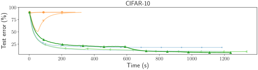
Figure F.2: VGG16 image classification benchmark with PyTorch solvers. The best SGD configuration features data augmentation, momentum, step learning rate schedule and weight decay.

In Figure F.2, we see that for the case of VGG, the application of weight decay is so important that without it, in cases with momentum, the model does not converge.

Appendix G $\ell_{1}$-regularized logistic regression

This additional benchmark is dedicated to $\ell_{1}$-regularized logistic regression, in the same setting as Section 3 but this time with an $\ell_{1}$-regularization for the parameters of the model:

$$\theta^{*}=\mathop{\mathrm{arg\,min}}_{\theta\in\mathbb{R}^{p}}\sum_{i=1}^{n}\log\big{(}1+\exp(-y_{i}X_{i}^{\top}\theta)\big{)}+\lambda\|\theta\|_{1}\enspace.$$ (2)

G.1 List of solvers and datasets used in the $\ell_{1}$-regularized logistic regression benchmark

The code for the benchmark is available at https://github.com/benchopt/benchmark_logreg_l1/. Table G.1 and Table G.2 present the solvers and datasets used in this benchmark.

Table G.1: List of solvers used in the $\ell_{1}$-regularized logistic regression benchmark

Solver	References	Description	Language
blitz	[76]	CD + working set	Python, C++
coordinate descent	[56]	(Cyclic) Minimization along coordinates	Python (Numba)
coordinate descent (Newton)	[56]	CD + Newton	Python (Numba)
celer	[98]	CD + working set + dual extrapolation	Python (Cython)
copt[FISTA line search]	[108], [8]	FISTA (ISTA + acceleration) + line search	Python (Cython)
copt[PGD]	[108], [37]	Proximal Gradient Descent	Python (Cython)
copt[PGD linesearch]	[108], [37]	Proximal Gradient Descent + linesearch	Python (Cython)
copt[saga]	[108]	SAGA (Variance reduced stochastic method)	Python (Cython)
copt[svrg]	[108]	SVRG (Variance reduced stochastic method)	Python (Cython)
cuML[gpu]	[120]	L-BFGS + GPU	Python, C++
cuML[qn]	[120]	Orthant-Wise Limited Memory Quasi-Newton (OWL-QN)	Python, C++
cyanure	[97]	Proximal Minimization by Incremental Surrogate Optimization (MISO)	Python, C++
lightning	[17]	(Cyclic) Coordinate Descent	Python (Cython)
scikit-learn[liblinear]	[109], [52]	Truncated Newton Conjugate-Gradient	Python (Cython)
scikit-learn[lbfgs]	[109], [139]	L-BFGS (Quasi-Newton Method)	Python (Cython)
scikit-learn[newton-cg]	[109], [139]	Truncated Newton Conjugate-Gradient	Python (Cython)
snapml[gpu=True]	[46]	CD + GPU	Python, C++
snapml[gpu=False]	[46]	CD	Python, C++

Table G.2: List of the datasets used in the $\ell_{1}$-regularized logistic regression benchmark

Datasets	References	Samples ($\mathbf{n}$)	Features ($\mathbf{p}$)	Density
gisette	[63]	$6000$	$5000$	$9.9\text{\times}{10}^{-1}$
colon-cancer	[63]	$62$	$2000$	$1.0$
news20.binary	[78]	$19\,996$	$1\,355\,191$	$0.000\,34$
rcv1.binary	[63]	$20\,242$	$19\,959$	$3.6\text{\times}{10}^{-3}$

G.2 Results

The results of the $\ell_{1}$-regularized logistic regression benchmark are in Figure G.1.

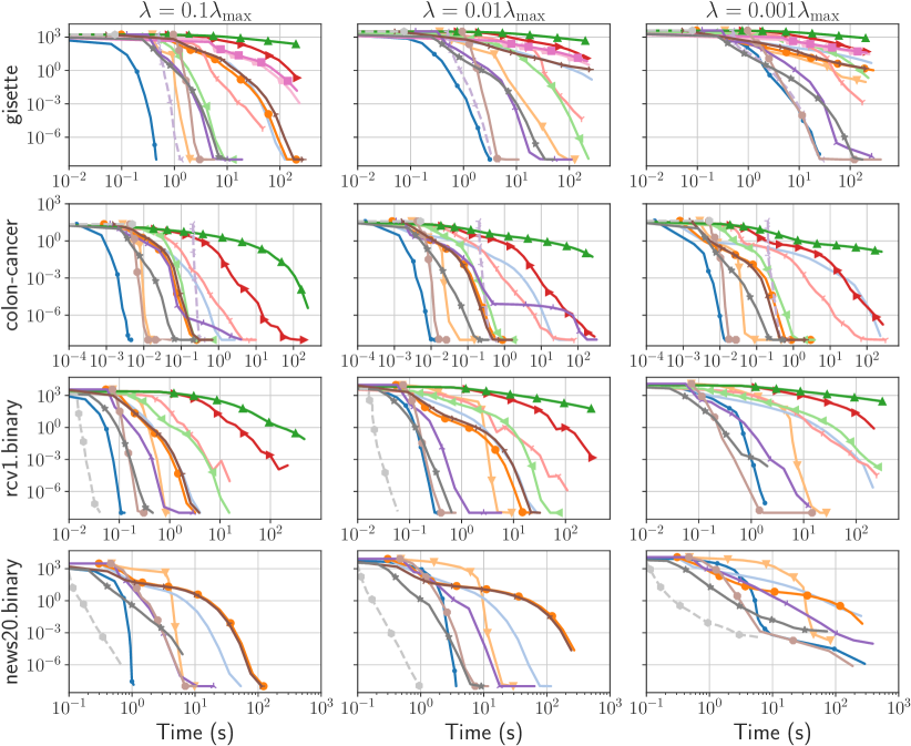
Figure G.1: Benchmark for the $\ell_{1}$-regularized logistic regression on variants of the Objective (columns). The curves display the suboptimality of the iterates, $f(\theta^{t})-f(\theta^{*})$, as a function of time. The first column corresponds to the objective detailed in Appendix G with $\lambda=0.1\|X^{\top}y\|_{\infty}/2$, the second one with $\lambda=0.01\|X^{\top}y\|_{\infty}/2$ and the third column with $\lambda=0.001\|X^{\top}y\|_{\infty}/2$.

Appendix H Unidimensional total variation

The use of 1D Total Variation regularization takes its root in the taut-string algorithm [6] and can be seen as a special case of either the Rudin-Osher-Fatemi model [124] or the Generalized Lasso [136] for a quadratic data fit term. It reads

$$\theta^{*}\in\mathop{\mathrm{arg\,min}}_{\theta\in\mathbb{R}^{p}}F(y,X\theta)+\lambda\left\|D\theta\right\|_{1}\enspace,$$ (2)

where $F$ is a data fidelity term, $X\in\mathbb{R}^{n\times p}$ is a design matrix with $n$ samples and $p$ features, $y\in\mathbb{R}^{n}$ is the target vector, $\lambda>0$ is a regularization hyperparameter, and $D\in\mathbb{R}^{(p-1)\times p}$ is a finite difference operator defined by $(D\theta)_{k}=\theta_{k+1}-\theta_{k}$ for all $1\leq k\leq p-1$ (it is also possible to use cyclic differences).

Most often, the data fidelity term is the $\ell^{2}$-loss $F(y,z)=\tfrac{1}{2}\left\|y-z\right\|_{2}^{2}$, following an additive Gaussian noise hypothesis. But the data fit term can also account for other types of noises, such as noises with heavy tails using the Huber loss $F(y,z)=|y-z|_{\mu}$ where $|\cdot|_{\mu}$ is defined coordinate-wise by

$$|t|_{\mu}=\begin{cases}\frac{1}{2}t^{2}&\textrm{if }|t|\leq\mu\\ \mu|t|-\frac{\mu^{2}}{2}&\textrm{otherwise.}\end{cases}$$

Appendix H promotes piecewise-constant solutions – alternatively said, solutions such that their gradients is sparse – and was proved to be useful in several applications, in particular for change point detection [16, 135], for BOLD signal deconvolution in functional MRI [77, 34] or for detrending in oculomotor recordings [87].

The penalty $\theta\mapsto\left\|D\theta\right\|_{1}$ is convex but non-smooth, and its proximity operator has no closed form. Yet as demonstrated by [39], the taut-string algorithm allows to compute this proximity operator in $O(p^{2})$ operations in the worst case, but it enjoys a $O(p)$ complexity in most cases. Other methods do not rely on this proximity operator and directly solve Appendix H, using either primal-dual approaches [32, 40], or solving the dual problem [83]. Finally, for 1-dimensional TV regularization, one can also use the synthesis formulation [49] to solve the problem. By setting $z=D\theta$ and $\theta=Lz+\rho$ where $L\in\mathbb{R}^{p\times p-1}$ is a lower trianglar matrix representing an integral operator (cumulative sum), the problem is equivalent to a Lasso problem, and $\rho^{*}$ has a closed-form expression (see e.g., [16] for a proof). As a consequence, any lasso solver can be used to obtain the solution of the Lasso problem $z^{*}$ and the solution of the original Appendix H $u^{*}$ is retrieved as $u^{*}=Lz^{*}+\rho^{*}$.

The code for the benchmark is available at https://github.com/benchopt/benchmark_tv_1d/ and Table H.1 details the different algorithms used in this benchmark.

Table H.1: List of solvers used in the 1D Total Variation benchmarks

Solver	References	Formulation	Description
ADMM	[22]	Analysis	Primal-Dual Augmented Lagrangian
ChambollePock	[32]	Analysis	Primal-Dual Hybrid Gradient
CondatVu	[40]	Analysis	Primal-Dual Hybrid Gradient
DPGD	[83]	Analysis	Dual proximal GD (+ acceleration)
PGD	[39]	Analysis	Proximal GD + taut–string
	[5]		ProxTV (+ acceleration)
celer	[98]	Synthesis	CD + working set (lasso)
			only for $\ell_{2}$ data-fit
FP	[38]	Synthesis	Fixed point with block updates
ISTA	[42]	Synthesis	Proximal GD (+ acceleration)
skglm	[13]	Synthesis	CD + working set

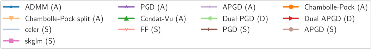
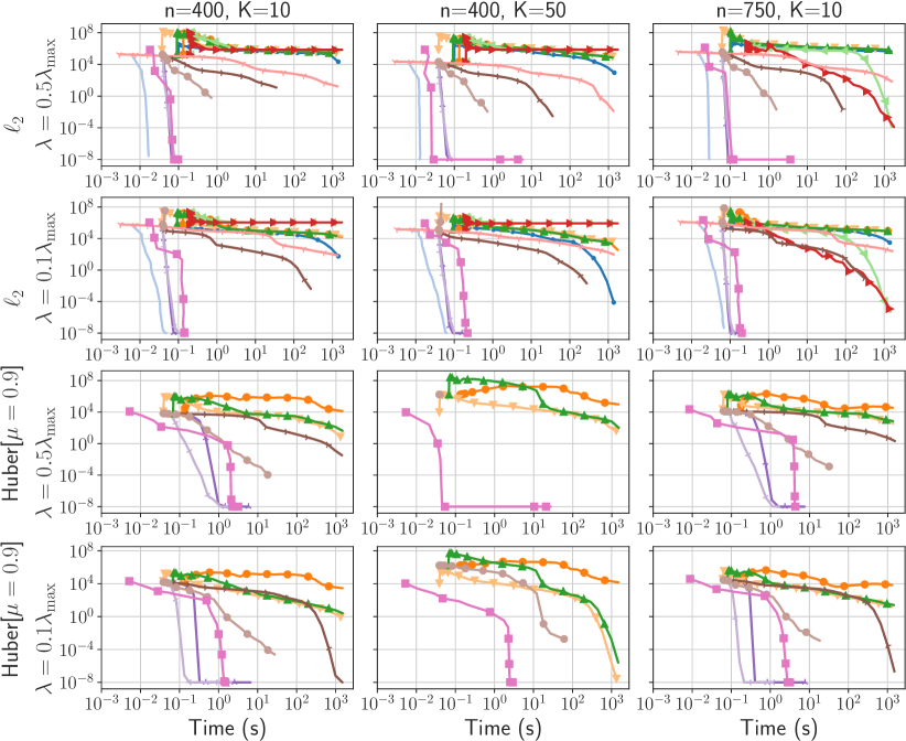
Figure H.1: Benchmark for the $TV$-regularized regression regression, on 13 solvers, 4 variants of the Objective (rows), and 3 configurations for a simulated dataset (columns). The curves display the suboptimality of the iterates, $f(\theta^{t})-f(\theta^{*})$, as a function of time. The solvers in this benchmark showcase the three resolution approaches with the Analysis (A), Dual (D) and Synthesis (S) formulations.

Simulated dataset   We use here simulated data, as applications based on fMRI and EOG signals require access to open and preprocessed data that we will make available on OpenML [138] in the future. The data are generated as follows: a block signal $\bar{\theta}\in\mathbb{R}^{p}$ is generated by sampling first a sparse random vector $z\in\mathbb{R}^{p}$ with $K$ non-zero coefficients positioned randomly, and taking random values following a $\mathcal{N}(0,1)$ distribution. Finally, $\bar{\theta}$ is obtained by discrete integration as $\bar{\theta}_{i}=\sum_{k=1}^{i}z_{k}$ for $1\leq i\leq p$. The design matrix $X\in\mathbb{R}^{n\times p}$ is a Gaussian random design with $X_{ij}\sim\mathcal{N}(0,1)$. The observations $y$ are obtained as $y=X\bar{\theta}+\epsilon$, with $\epsilon\sim\mathcal{N}(0,0.01)$ a Gaussian white noise. For all experiments, we used $p=500$ and vary the number of non-zero coefficient $K$, and the number of rows $n$ of the matrix $X$.

Results   Figure H.1 shows that the solvers using the synthesis formulation and coordinate descent-based solvers for the Lasso ($\ell_{2}$ data fit term) work best on this type of problem. For the Huber data fit term, the solver using the analysis formulation and the taut-string algorithm for the proximal operator are faster. An interesting observation from this benchmark is the behavior of the solvers based on primal-dual splitting or dual formulation. We observe that for all these solvers, the objective starts by increasing. This is probably due to a sub-optimal initialization of the dual variable compared to the primal one. While this initialization is seldom described in the literature, it seems to have a large impact on the speed of these algorithms. This shows how Benchopt allows to reveal such behavior, and could lead to practical guidelines on how to select this dual initialization.

Extensions   We plan to extend this benchmark in the future to consider higher dimensional problems – e.g.,  2D TV problems for images – or higher order TV regularization, such as Total Generalized Variation [26] or inf-convolution of TV functionals [31] – used of instance for change point detection [135]. Yet, for 2D or higher dimensional problems, we can no longer use the synthesis formulation. It is however possible to apply the taut-string method of [39] and graph-cut methods of [24] and [82] for anisotropic TV, and dual or primal-dual methods for isotropic, such as Primal-Dual Hybrid Gradient algorithm [32].

Appendix I Linear regression with minimax concave penalty (MCP)

The Lasso problem [134] is a least-squares regression problem with a convex non-smooth penalty that induces sparsity in its solution. However, despite its success and large adoption by the machine learning and signal processing communities, it is plagued with some statistical drawbacks, such as bias for large coefficients. To overcome these issues, the standard approach is to consider non-convex sparsity-inducing penalties. Several penalties have been proposed: Smoothly Clipped Absolute Deviation (SCAD, [51]), the Log Sum penalty [30], the capped-$\ell_{1}$ penalty [146] or the Minimax Concave Penalty (MCP, [144]).

This benchmark is devoted to least-squares regression with the latter, namely the problem:

$$\theta^{*}\in\mathop{\mathrm{arg\,min}}_{\theta\in\mathbb{R}^{p}}\tfrac{1}{2n}\left\|y-X\theta\right\|^{2}+\sum_{j=1}^{p}\rho_{\lambda,\gamma}(\theta_{j})\enspace,$$ (2)

where $X\in\mathbb{R}^{n\times p}$ is a design matrix containing $p$ features as columns, $y\in\mathbb{R}^{n}$ is the target vector, and $\rho_{\lambda,\gamma}$ the penalty function that reads as:

$$\rho_{\lambda,\gamma}(t)=\begin{cases}\lambda|t|-\frac{t^{2}}{2\gamma}\enspace,\quad&\text{if }|t|\leq\gamma\lambda\enspace,\\ \frac{\lambda^{2}\gamma}{2}\enspace,\quad&\text{if }|t|>\gamma\lambda\enspace.\end{cases}$$

Similarly to the Lasso, Appendix I promotes sparse solutions but the optimization problem raises some difficulties due to the non-convexity and non-smoothness of the penalty. Nonetheless, several efficient algorithms have been derived for solving it. The ones we use in the benchmark are listed in Table I.1.

Table I.1: List of solvers used in the MCP benchmark

Solver	References	Short Description
CD	[27], [100]	Proximal coordinate descent
PGD	[19]	Proximal gradient descent
GIST	[60]	Proximal gradient + Barzilai-Borwein rule
WorkSet CD	[18]	Coordinate descent + working set
skglm	[13]	Accelerated coordinate descent + Working set

The code for the benchmark is available at https://github.com/benchopt/benchmark_mcp/. For this benchmark, we run the solvers on the colon-cancer dataset and on the simulated dataset described in Table B.1. We use a signal-to-noise ratio $\texttt{snr}=3$, a correlation $\rho=0.6$ with $n=500$ observations and $p=2000$ features.

I.1 Results

The result of the benchmark is presented in Figure I.1 The problem is non-convex and solvers are only guaranteed to converge to local minima; hence in Figure I.1 we monitor the distance of the negative gradient to the Fréchet subdifferential of the MCP, representing the violation of the first order optimality condition. Other metrics, such as objective of iterates sparsity, are monitored in the full benchmark, allowing to compare the different limit points obtained by the solvers.

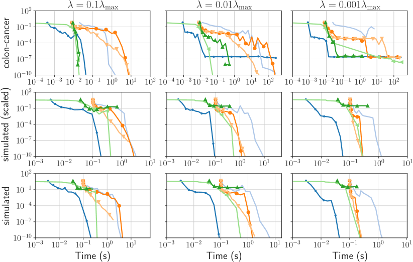
Figure I.1: Benchmark for the MCP regression on variants of the Objective (columns). The curves display the violation of optimality conditions, $\operatorname{dist}(-X^{\top}(X\theta_{t}-y)/n,\partial\rho_{\lambda,\gamma}(\theta_{t}))$, as a function of time. $\gamma$ is set to 3, and $\lambda$ is parameterized as a fraction of the Lasso’s $\lambda_{\max}$, $\left\|X^{\top}y\right\|_{\infty}/n$.

Appendix J Zero-order optimization on standard functions

Zero-order optimization refers to scenarios where only calls to the function to minimize are possible. This is in contrast with first-order optimization where gradient information is available. Grid search, random search, evolution strategies (ES) or Bayesian optimization (BO) are popular methods to tackle such a problem and are most commonly employed for hyperparameter optimization. This setting is also known as black-box optimization.

This benchmark demonstrates the usability of Benchopt for zero-order optimization considering functions classically used in the literature [64]. The functions are available in the PyBenchFCN package https://github.com/Y1fanHE/PyBenchFCN/. In particular, among the 61 functions of interest we present here (see Figure J.1) a benchmark for three functions, defined for any $\mathbf{x}=(x_{1},\ldots,x_{N})\in\mathbb{R}^{N}$:

$$f(\mathbf{x}) =\sum_{i=1}^{N-1}[100(x_{i+1}-x_{i}^{2})^{2}+(1-x_{i})^{2}]\,$$ (Rosenbrock)

$$f(\mathbf{x}) =10\cdot N+\sum_{i=1}^{N}[(x_{i}^{2}-10\cdot\cos(2\pi x_{i})]\,$$ (Rastrigin)

$$f(\mathbf{x}) =-20\cdot\exp\left[-0.2{\sqrt{\frac{1}{d}\sum_{i=1}^{N}x_{i}^{2}}}\right]-\exp\left[{\frac{1}{d}\sum_{i=1}^{N}\cos(2\pi x_{i})}\right]+e+20\, \text{(Ackley)}\enspace.$$

For each function, the domain is restricted to a box: $\|\mathbf{x}\|_{\infty}\leq 32$ for Ackley, $\|\mathbf{x}\|_{\infty}\leq 30$ for Rosenbrock and $\|\mathbf{x}\|_{\infty}\leq 5.12$ for Rastrigin. The algorithms considered in the benchmark are listed in Table J.1. As BFGS requires first-order information, gradients are approximated with finite-differences.

Table J.1: List of solvers used in the zero-order benchmark

Solver	References	Description
Basin-hopping	[140, 139]	Two-phase method: global step + local min.
Nevergrad-RandomSearch	[119, 10]	Sampler by random search
Nevergrad-CMA	[119, 65]	CMA evolutionary strategy
Nevergrad-TwoPointsDE	[119]	Evolutionary strategy
Nevergrad-NGOpt	[119]	Adaptive evolutionary algorithm
Nelder-Mead	[57, 139]	Direct search (downhill simplex)
BFGS	[139]	BFGS with finite differences
Powell	[113, 139]	Conjugate direction method
optuna-TPE	[2, 11]	Sampler by Tree Parzen Estimation (TPE)
optuna-CMA	[2, 65]	CMA evolutionary strategy

The code for the benchmark is available at https://github.com/benchopt/benchmark_zero_order/.

J.1 Results

The results of the benchmark are presented in Figure J.1. The functions are non-convex and solvers are only guaranteed to converge to local minima; hence in Figure J.1 we monitor the value of the function. The functions are designed such that the global minimum of the function is always 0. One can observe that the CMA and TwoPointsDE implementations from nevergrad consistently reaches the global minimum. In addition, the CMA implementation from optuna is a bit slower than the one from nevergrad. Also one can notice that random search offers reasonable results. The TPE method seems to suffer from the curse of dimensionality, as most kernel methods in non-parametric estimation. Finally regarding the scipy solvers, Powell can be competitive, while Nelder-Mead and BFGS suffer a lot from local minima.

Figure J.1: Benchmark for the zero-order optimization on the Ackley, Rosenbrock and Rastrigin functions in dimension $N=20$.

References

- [1] Martín Abadi, Ashish Agarwal, Paul Barham, Eugene Brevdo, Zhifeng Chen, Craig Citro, Soprano Corrado, Andy Davis, Jeffrey Dean, Matthieu Devin, Sanjay Ghemawat, Ian Goodfellow, Andrew Harp, Geoffrey Irving, Michael Isard, Yangqing Jia, Rafal Jozefowicz, Lukasz Kaiser, Manjunath Kudlur, Josh Levenberg, D. Mané, Rajat Monga, Sherry Moore, Derek Murray, Chris Olah, Mike Schuster, Jonathon Shlens, Benoit Steiner, Ilya Sutskever, Kunal Talwar, Paul Tucker, Vincent Vanhoucke, Vijay Vasudevan, Fernanda Viégas, Oriol Vinyals, Pete Warden, Martin Wattenberg, Martin Wicke, Yuan Yu and Xiaoqiang Zheng “TensorFlow: Large-Scale Machine Learning on Heterogeneous Systems” Software available from tensorflow.org, 2015
- [2] Takuya Akiba, Shotaro Sano, Toshihiko Yanase, Takeru Ohta and Masanori Koyama “Optuna: A Next-generation Hyperparameter Optimization Framework” arXiv, 2019 DOI: 10.48550/ARXIV.1907.10902
- [3] Francis Bach, Rodolphe Jenatton, Julien Mairal and Guillaume Obozinski “Optimization with sparsity-inducing penalties” In Foundations and Trends in Machine Learning 4.1, 2012, pp. 1–106
- [4] E. Bacry, M. Bompaire, S. Gaïffas and S. Poulsen “Tick: A Python Library for Statistical Learning, with a Particular Emphasis on Time-Dependent Modeling” In ArXiv e-prints, 2017 eprint: 1707.03003
- [5] Alvero Barbero and Suvrit Sra “Modular Proximal Optimization for Multidimensional Total-Variation Regularization” In Journal of Machine Learning Research 19.56, 2018, pp. 1–82 URL: http://jmlr.org/papers/v19/13-538.html
- [6] R.. Barlow and H.. Brunk “The Isotonic Regression Problem and Its Dual” In Journal of the American Statistical Association 67.337 [American Statistical Association, Taylor & Francis, Ltd.], 1972, pp. 140–147
- [7] T. Bartz-Beielstein, C. Doerr, D. Berg, J. Bossek, S. Chandrasekaran, T. Eftimov, A. Fischbach, P. Kerschke, W. La Cava and M. Lopez-Ibanez “Benchmarking in optimization: Best practice and open issues” In arXiv preprint arXiv:2007.03488, 2020
- [8] A. Beck and M. Teboulle “A fast iterative shrinkage-thresholding algorithm for linear inverse problems” In SIAM J. Imaging Sci. 2.1, 2009, pp. 183–202
- [9] I. Bello, W. Fedus, X. Du, E.. Cubuk, A. Srinivas, T.-Y. Lin, J. Shlens and B. Zoph “Revisiting ResNets: Improved Training and Scaling Strategies” In Advances in Neural Information Processing Systems, 2021 arXiv:2103.07579v1
- [10] J. Bergstra and Y. Bengio “Random search for hyper-parameter optimization” In J. Mach. Learn. Res. 13.2, 2012
- [11] James Bergstra, Daniel Yamins and David Cox “Making a Science of Model Search: Hyperparameter Optimization in Hundreds of Dimensions for Vision Architectures” In ICML 28.1, 2013, pp. 115–123
- [12] Thierry Bertin-Mahieux, Daniel P.W. Ellis, Brian Whitman and Paul Lamere “The Million Song Dataset” In Proceedings of the 12th International Conference on Music Information Retrieval (ISMIR 2011), 2011
- [13] Q. Bertrand, Q. Klopfenstein, P.-A. Bannier, G. Gidel and M. Massias “Beyond L1: Faster and Better Sparse Models with skglm” In arXiv preprint arXiv:2204.07826, 2022
- [14] D.. Bertsekas “Nonlinear programming” Athena Scientific, 1999
- [15] Jeff Bezanson, Alan Edelman, Stefan Karpinski and Viral B Shah “Julia: A fresh approach to numerical computing” In SIAM Review 59.1 SIAM, 2017, pp. 65–98 DOI: 10.1137/141000671
- [16] Kevin Bleakley and Jean-Philippe Vert “The group fused Lasso for multiple change-point detection” arXiv, 2011
- [17] Mathieu Blondel and Fabian Pedregosa “Lightning: Large-Scale Linear Classification, Regression and Ranking in Python”, 2016
- [18] A. Boisbunon, R. Flamary and A. Rakotomamonjy “Active set strategy for high-dimensional non-convex sparse optimization problems” In ICASSP, 2014, pp. 1517–1521 IEEE
- [19] Jérôme Bolte, Shoham Sabach and Marc Teboulle “Proximal alternating linearized minimization for nonconvex and nonsmooth problems” In Mathematical Programming 146.1 Springer, 2014, pp. 459–494
- [20] A. Bonnefoy, V. Emiya, L. Ralaivola and R. Gribonval “Dynamic screening: accelerating first-order algorithms for the Lasso and Group-Lasso” In IEEE Trans. Signal Process. 63.19, 2015, pp. 20
- [21] Léon Bottou “Large-Scale Machine Learning with Stochastic Gradient Descent” In COMPSTAT Physica-Verlag, 2010, pp. 177–186
- [22] Stephen Boyd, Neal Parikh, Eric Chu, Borja Peleato and Jonathan Eckstein “Distributed Optimization and Statistical Learning via the Alternating Direction Method of Multipliers” In Foundations and Trends in Machine Learning 3.1, 2011
- [23] Stephen P. Boyd and Lieven Vandenberghe “Convex Optimization” Cambridge, UK ; New York: Cambridge University Press, 2004
- [24] Y. Boykov, O. Veksler and R. Zabih “Fast approximate energy minimization via graph cuts” In IEEE Transactions on Pattern Analysis and Machine Intelligence 23.11, 2001, pp. 1222–1239 DOI: 10.1109/34.969114
- [25] Georg Brandl “Sphinx documentation” In URL http://sphinx-doc. org/sphinx. pdf, 2010
- [26] Kristian Bredies, Karl Kunisch and Thomas Pock “Total generalized variation” In SIAM J. Imaging Sci. 3.3 SIAM, 2010, pp. 492–526
- [27] P. Breheny and J. Huang “Coordinate descent algorithms for nonconvex penalized regression, with applications to biological feature selection” In Ann. Appl. Stat. 5.1 NIH Public Access, 2011, pp. 232
- [28] A. Brock, S. De, S.. Smith and K. Simonyan “High-performance large-scale image recognition without normalization” In ICML, 2021, pp. 1059–1071 PMLR
- [29] P. Bühlmann and S. van de Geer “Statistics for high-dimensional data” Methods, theory and applications, Springer Series in Statistics Heidelberg: Springer, 2011
- [30] E.. Candès, M.. Wakin and S.. Boyd “Enhancing Sparsity by Reweighted Minimization” In J. Fourier Anal. Applicat. 14.5-6, 2008, pp. 877–905
- [31] Antonin Chambolle and Pierre-Louis Lions “Image recovery via total variation minimization and related problems” In Numerische Mathematik 76.2 Springer, 1997, pp. 167–188
- [32] Antonin Chambolle and Thomas Pock “A first-order primal-dual algorithm for convex problems with applications to imaging” In Journal of Mathematical Imaging and Vision 40.1, 2011
- [33] S.. Chen, D.. Donoho and M.. Saunders “Atomic decomposition by basis pursuit” In SIAM J. Sci. Comput. 20.1, 1998, pp. 33–61
- [34] Hamza Cherkaoui, Thomas Moreau, Abderrahim Halimi and Philippe Ciuciu “Sparsity-Based Semi-Blind Deconvolution of Neural Activation Signal in fMRI” In IEEE International Conference on Acoustics, Speech and Signal Processing (ICASSP), 2019
- [35] Francois Chollet “Keras” GitHub, 2015
- [36] Alex Clark “Pillow (PIL Fork) Documentation” readthedocs, 2015 URL: https://buildmedia.readthedocs.org/media/pdf/pillow/latest/pillow.pdf
- [37] P.. Combettes and V. Wajs “Signal recovery by proximal forward-backward splitting” In Multiscale modeling & simulation 4.4 SIAM, 2005, pp. 1168–1200
- [38] Patrick L. Combettes and Lilian E. Glaudin “Solving Composite Fixed Point Problems with Block Updates” In Advances in Nonlinear Analysis, 2021
- [39] Laurent Condat “A Direct Algorithm for 1-D Total Variation Denoising” In IEEE SIGNAL PROCESSING LETTERS 20.12, 2013
- [40] Laurent Condat “A primal-dual splitting method for convex optimization involving Lipschitzian, proximable and linear composite terms” In Journal of Optimization Theory and Applications, Springer Verlag, 2013
- [41] Criteo-Labs “Criteo releases industry’s largest-ever dataset for machine learning to academic community”, 2015 URL: https://www.criteo.com/news/press-releases/2015/07/criteo-releases-industrys-largest-ever-dataset
- [42] I. Daubechies, M. Defrise and C. De Mol “An iterative thresholding algorithm for linear inverse problems with a sparsity constraint” In Commun. Pure Appl. Math. 57.11 Wiley Online Library, 2004, pp. 1413–1457
- [43] Aaron Defazio, Francis Bach and Simon Lacoste-Julien “SAGA: A Fast Incremental Gradient Method With Support for Non-Strongly Convex Composite Objectives” In Advances in Neural Information Processing Systems 28, 2014, pp. 1646–1654
- [44] Ron S Dembo, Stanley C Eisenstat and Trond Steihaug “Inexact Newton Methods” In SIAM J. Numer. Anal. 19.2 SIAM, 1982, pp. 400–408
- [45] Alexey Dosovitskiy, Lucas Beyer, Alexander Kolesnikov, Dirk Weissenborn, Xiaohua Zhai, Thomas Unterthiner, Mostafa Dehghani, Matthias Minderer, Georg Heigold, Sylvain Gelly, Jakob Uszkoreit and Neil Houlsby “An Image is Worth 16x16 Words: Transformers for Image Recognition at Scale” In ICLR, 2021
- [46] C. Dünner, T. Parnell, D. Sarigiannis, N. Ioannou, A. Anghel, G. Ravi, M. Kandasamy and H. Pozidis “Snap ML: A hierarchical framework for machine learning” In Advances in Neural Information Processing Systems 31, 2018
- [47] B. Efron, T.. Hastie, I.. Johnstone and R. Tibshirani “Least angle regression” With discussion, and a rejoinder by the authors In Ann. Statist. 32.2, 2004, pp. 407–499
- [48] L. El Ghaoui, V. Viallon and T. Rabbani “Safe feature elimination in sparse supervised learning” In J. Pacific Optim. 8.4, 2012, pp. 667–698
- [49] Michael Elad, Peyman Milanfar and Ron Rubinstein “Analysis versus synthesis in signal priors” In 2006 14th European Signal Processing Conference, 2006
- [50] William Falcon, Jirka Borovec, Adrian Wälchli, Nic Eggert, Justus Schock, Jeremy Jordan, Nicki Skafte, Ir1dXD, Vadim Bereznyuk, Ethan Harris, Tullie Murrell, Peter Yu, Sebastian Præsius, Travis Addair, Jacob Zhong, Dmitry Lipin, So Uchida, Shreyas Bapat, Hendrik Schröter, Boris Dayma, Alexey Karnachev, Akshay Kulkarni, Shunta Komatsu, Martin.B, Jean-Baptiste SCHIRATTI, Hadrien Mary, Donal Byrne, Cristobal Eyzaguirre, cinjon and Anton Bakhtin “PyTorchLightning/pytorch-lightning: 0.7.6 release” Zenodo, 2020
- [51] J. Fan and R. Li “Variable selection via nonconcave penalized likelihood and its oracle properties” In J. Amer. Statist. Assoc. 96.456, 2001, pp. 1348–1360
- [52] Rong-En Fan, Kai-Wei Chang, Cho-Jui Hsieh, Xiang-Rui Wang and Chih-Jen Lin “LIBLINEAR: A Library for Large Linear Classification” In J. Mach. Learn. Res. 9 Cambridge, MA, USA: MIT Press, 2008
- [53] S Farrens, A Grigis, L El Gueddari, Z Ramzi, GR Chaithya, S Starck, B Sarthou, H Cherkaoui, P Ciuciu and J-L Starck “PySAP: Python Sparse Data Analysis Package for multidisciplinary image processing” In Astronomy and Computing 32 Elsevier, 2020, pp. 100402
- [54] R. Fletcher and C.. Reeves “Function Minimization by Conjugate Gradients” In The Computer Journal 7.2, 1964, pp. 149–154 eprint: https://academic.oup.com/comjnl/article-pdf/7/2/149/959725/070149.pdf
- [55] J. Forde, T. Head, C. Holdgraf, Y. Panda, G. Nalvarete, B. Ragan-Kelley and E. Sundell “Reproducible research environments with repo2docker”, 2018
- [56] J. Friedman, T. Hastie and R. Tibshirani “Regularization paths for generalized linear models via coordinate descent” In J. Stat. Softw. 33.1 NIH Public Access, 2010, pp. 1–22
- [57] Fuchang Gao and Lixing Han “Implementing the Nelder-Mead simplex algorithm with adaptive parameters” In Computational Optimization and Applications 51.1 Springer, 2012, pp. 259–277
- [58] X. Glorot and Y. Bengio “Understanding the difficulty of training deep feedforward neural networks” In AISTATS 9, 2010, pp. 249–256
- [59] Todd R Golub, Donna K Slonim, Pablo Tamayo, Christine Huard, Michelle Gaasenbeek, Jill P Mesirov, Hilary Coller, Mignon L Loh, James R Downing and Mark A Caligiuri “Molecular classification of cancer: class discovery and class prediction by gene expression monitoring” In science 286.5439 American Association for the Advancement of Science, 1999, pp. 531–537
- [60] P. Gong, C. Zhang, Z. Lu, J. Huang and J. Ye “A general iterative shrinkage and thresholding algorithm for non-convex regularized optimization problems” In ICML, 2013, pp. 37–45
- [61] A. Gramfort, M. Luessi, E. Larson, D.. Engemann, D. Strohmeier, C. Brodbeck, L. Parkkonen and M.. Hämäläinen “MNE software for processing MEG and EEG data” In NeuroImage 86, 2014, pp. 446–460
- [62] Y. Grandvalet “Least absolute shrinkage is equivalent to quadratic penalization” In International Conference on Artificial Neural Networks, 1998, pp. 201–206 Springer
- [63] Isabelle Guyon, Steve Gunn, Asa Ben-Hur and Gideon Dror “Result analysis of the nips 2003 feature selection challenge” In Advances in neural information processing systems 17, 2004
- [64] Nikolaus Hansen, Anne Auger, Raymond Ros, Olaf Mersmann, Tea Tušar and Dimo Brockhoff “COCO: A Platform for Comparing Continuous Optimizers in a Black-Box Setting” ArXiv e-prints, arXiv:1603.08785 In Optimization Methods and Software 36.1 Taylor & Francis, 2021, pp. 114–144 DOI: 10.1080/10556788.2020.1808977
- [65] Nikolaus Hansen and Andreas Ostermeier “Completely derandomized self-adaptation in evolution strategies” In Evolutionary computation 9.2 MIT Press, 2001, pp. 159–195
- [66] Charles R Harris, K Jarrod Millman, Stéfan J Van Der Walt, Ralf Gommers, Pauli Virtanen, David Cournapeau, Eric Wieser, Julian Taylor, Sebastian Berg and Nathaniel J Smith “Array programming with NumPy” In Nature 585.7825 Nature Publishing Group, 2020, pp. 357–362
- [67] T.. Hastie, R. Tibshirani and M. Wainwright “Statistical Learning with Sparsity: The Lasso and Generalizations” CRC Press, 2015
- [68] Kaiming He, Xiangyu Zhang, Shaoqing Ren and Jian Sun “Delving deep into rectifiers: Surpassing human-level performance on imagenet classification” In CVPR, 2015, pp. 1026–1034
- [69] Kaiming He, Xiangyu Zhang, Shaoqing Ren and Jian Sun “Deep residual learning for image recognition” In CVPR, 2016
- [70] Tong He, Zhi Zhang, Hang Zhang, Zhongyue Zhang, Junyuan Xie and Mu Li “Bag of tricks for image classification with convolutional neural networks” In CVPR 2019-June, 2019, pp. 558–567 arXiv:1812.01187
- [71] J.. Hunter “Matplotlib: A 2D graphics environment” In Computing in Science & Engineering 9.3 IEEE COMPUTER SOC, 2007, pp. 90–95 DOI: 10.1109/MCSE.2007.55
- [72] M. Hutson “Artificial intelligence faces reproducibility crisis” In Science 359.6377 American Association for the Advancement of Science, 2018, pp. 725–726
- [73] Plotly Technologies Inc. “Collaborative data science” Montreal, QC: Plotly Technologies Inc., 2015 URL: https://plot.ly
- [74] S. Ioffe and C. Szegedy “Batch normalization: Accelerating deep network training by reducing internal covariate shift” In ICML, 2015, pp. 448–456
- [75] Rie Johnson and Tong Zhang “Accelerating Stochastic Gradient Descent Using Predictive Variance Reduction” In Advances in Neural Information Processing Systems 26, 2013
- [76] T.. Johnson and C. Guestrin “Blitz: A Principled Meta-Algorithm for Scaling Sparse Optimization” In ICML 37, 2015, pp. 1171–1179
- [77] Fikret Işık Karahanoğlu, César Caballero-Gaudes, François Lazeyras and Dimitri Van De Ville “Total Activation: fMRI Deconvolution through Spatio-Temporal Regularization” In NeuroImage 73, 2013, pp. 121–134
- [78] S Sathiya Keerthi, Dennis DeCoste and Thorsten Joachims “A modified finite Newton method for fast solution of large scale linear SVMs.” In Journal of Machine Learning Research 6.3, 2005
- [79] Jack Kiefer and Jacob Wolfowitz “Stochastic estimation of the maximum of a regression function” In Ann. Math. Stat., 1952, pp. 462–466
- [80] Diederik P. Kingma and Jimmy Ba “Adam: A Method for Stochastic Optimization” In ICLR, 2015, pp. 1–10
- [81] K. Koh, J. Kim and S. Boyd “An interior-point method for large-scale l1-regularized logistic regression.” In J. Mach. Learn. Res. 8.8, 2007, pp. 1519–1555
- [82] V. Kolmogorov and R. Zabin “What energy functions can be minimized via graph cuts?” In IEEE Transactions on Pattern Analysis and Machine Intelligence 26.2, 2004, pp. 147–159 DOI: 10.1109/TPAMI.2004.1262177
- [83] Nikos Komodakis and Jean-Christophe Pesquet “Playing with Duality: An overview of recent primal-dual approaches for solving large-scale optimization problems” In IEEE Signal Processing Magazine, Institute of Electrical and Electronics Engineers, 2015
- [84] Simon Kornblith “Lasso.jl”, 2021 JuliaStats URL: https://github.com/JuliaStats/Lasso.jl
- [85] Alex Krizhevsky “Learning multiple layers of features from tiny images”, 2009
- [86] Alex Krizhevsky, Ilya Sutskever and Geoffrey E. Hinton “Imagenet Classification with Deep Convolutional Neural Networks” In Advances in Neural Information Processing Systems, 2012, pp. 1097–1105
- [87] Clement Lalanne, Maxence Rateaux, Laurent Oudre, Matthieu P. Robert and Thomas Moreau “Extraction of Nystagmus Patterns from Eye-Tracker Data with Convolutional Sparse Coding” In Annual International Conference of the IEEE Engineering in Medicine & Biology Society (EMBC) Montreal, QC, Canada: IEEE, 2020, pp. 928–931
- [88] Yann LeCun, Corinna Cortes and CJ Burges “MNIST handwritten digit database” In ATT Labs [Online]. Available: http://yann.lecun.com/exdb/mnist 2, 2010
- [89] David D Lewis, Yiming Yang, Tony Russell-Rose and Fan Li “Rcv1: A new benchmark collection for text categorization research” In Journal of machine learning research 5.Apr Goldsmiths, University of London, 2004, pp. 361–397
- [90] Jingwei Liang, Tao Luo and Carola-Bibiane Schöenlieb “Improving “Fast Iterative Shrinkage-Thresholding Algorithm”: Faster, Smarter, and Greedier” In SIAM J. Sci. Comput. 44.3 SIAM, 2022, pp. A1069–A1091
- [91] Dong C. Liu and Jorge Nocedal “On the Limited Memory BFGS Method for Large Scale Optimization” In Math. Program. 45.1-3, 1989, pp. 503–528
- [92] Zhuang Liu, Hanzi Mao, Chao-Yuan Wu, Christoph Feichtenhofer, Trevor Darrell and Saining Xie “A ConvNet for the 2020s” In CVPR, 2022
- [93] Ilya Loshchilov and Frank Hutter “SGDR: Stochastic Gradient Descent with Warm Restarts” In ICLR, 2017
- [94] Ilya Loshchilov and Frank Hutter “Decoupled Weight Decay Regularization” In ICLR, 2019
- [95] Jan-Matthis Lueckmann, Jan Boelts, David S Greenberg, Pedro J Gonçalves and Jakob H Macke “Benchmarking Simulation-Based Inference” In AISTATS 130, PMLR, 2021, pp. 343–351
- [96] J. Mairal and B. Yu “Complexity analysis of the Lasso regularization path” In ICML, 2012, pp. 353–360
- [97] Julien Mairal “Cyanure: An open-source toolbox for empirical risk minimization for python, c++, and soon more” In arXiv preprint arXiv:1912.08165, 2019
- [98] M. Massias, A. Gramfort and J. Salmon “Celer: a fast solver for the lasso with dual extrapolation” In ICML, 2018, pp. 3315–3324
- [99] P. Mattson, V. Reddi, C. Cheng, C. Coleman, G. Diamos, D. Kanter, P. Micikevicius, D. Patterson, G. Schmuelling and H. Tang “MLPerf: An industry standard benchmark suite for machine learning performance” In IEEE Micro 40.2 IEEE, 2020, pp. 8–16
- [100] R. Mazumder, J.. Friedman and T. Hastie “Sparsenet: Coordinate descent with nonconvex penalties” In J. Amer. Statist. Assoc. 106.495 Taylor & Francis, 2011, pp. 1125–1138
- [101] Wes McKinney “Data structures for statistical computing in python” In Proceedings of the 9th Python in Science Conference 445, 2010, pp. 51–56 Austin, TX
- [102] Thomas Moreau, Pierre Glaser, Roman Yurchak and Olivier Grisel “Loky”, 2017 DOI: 10.5281/zenodo.5770406
- [103] Óscar Nájera, Eric Larson, Loïc Estève, Gael Varoquaux, Lucy Liu, Jaques Grobler, Elliott Sales Andrade, Chris Holdgraf, Alexandre Gramfort, Mainak Jas, Joel Nothman, Olivier Grisel, Nelle Varoquaux, Emmanuelle Gouillart, Martin Luessi, Antony Lee, Jake Vanderplas, Tim Hoffmann, Thomas A Caswell, Bane Sullivan, Alyssa Batula, jaeilepp, Thomas Robitaille, Stefan Appelhoff, Patrick Kunzmann, Matthias Geier, Lars, Kyle Sunden, Dominik Stańczak and Albert Y. Shih “sphinx-gallery/sphinx-gallery: Release v0.7.0” Zenodo, 2020 DOI: 10.5281/zenodo.3838216
- [104] E. Ndiaye, O. Fercoq, A. Gramfort and J. Salmon “Gap Safe screening rules for sparsity enforcing penalties” In J. Mach. Learn. Res. 18.128, 2017, pp. 1–33
- [105] Yurii E Nesterov “A method for solving the convex programming problem with convergence rate ” In Dokl. akad. nauk Sssr 269, 1983, pp. 543–547
- [106] Yuval Netzer, Tao Wang, Adam Coates, Alessandro Bissacco, Bo Wu and Andrew Y Ng “Reading Digits in Natural Images with Unsupervised Feature Learning” In Advances in Neural Information Processing Systems, 2011
- [107] Adam Paszke, Sam Gross, Francisco Massa, Adam Lerer, James Bradbury, Gregory Chanan, Trevor Killeen, Zeming Lin, Natalia Gimelshein, Luca Antiga, Alban Desmaison, Andreas Kopf, Edward Yang, Zachary DeVito, Martin Raison, Alykhan Tejani, Sasank Chilamkurthy, Benoit Steiner, Lu Fang, Junjie Bai and Soumith Chintala “PyTorch: An Imperative Style, High-Performance Deep Learning Library” In Advances in Neural Information Processing Systems, 2019, pp. 8024–8035
- [108] Fabian Pedregosa, Geoffrey Negiar and Gideon Dresdner “copt: composite optimization in Python”, 2020
- [109] Fabian Pedregosa, Gaël Varoquaux, Alexandre Gramfort, Vincent Michel, Bertrand Thirion, Olivier Grisel, Mathieu Blondel, Peter Prettenhofer, Ron Weiss and Vincent Dubourg “Scikit-learn: Machine learning in Python” In J. Mach. Learn. Res. 12 JMLR. org, 2011, pp. 2825–2830
- [110] J. Pineau, P. Vincent-Lamarre, K. Sinha, V. Larivière, A. Beygelzimer, F. d’Alché-Buc, E. Fox and H. Larochelle “Improving reproducibility in machine learning research: a report from the NeurIPS 2019 reproducibility program” In J. Mach. Learn. Res. 22 Microtome Publishing, 2021
- [111] Joelle Pineau, Koustuv Sinha, Genevieve Fried, Rosemary Nan Ke and Hugo Larochelle “ICLR reproducibility challenge 2019” In ReScience C 5.2, 2019, pp. 5
- [112] Clarice Poon and Gabriel Peyré “Smooth Bilevel Programming for Sparse Regularization” In Advances in Neural Information Processing Systems 34, 2021, pp. 1543–1555
- [113] Michael JD Powell “An efficient method for finding the minimum of a function of several variables without calculating derivatives” In The computer journal 7.2 Oxford University Press, 1964, pp. 155–162
- [114] William H Press, Saul A Teukolsky, William T Vetterling and Brian P Flannery “Numerical recipes 3rd edition: The art of scientific computing” Cambridge university press, 2007
- [115] Danil Prokhorov “IJCNN 2001 neural network competition” In Slide presentation in IJCNN 1.97, 2001, pp. 38
- [116] Emmanuel Quemener and Marianne Corvellec “SIDUS—the solution for extreme deduplication of an operating system” In Linux Journal 2013.235 Belltown Media Houston, TX, 2013, pp. 3
- [117] R Core Team “R: A Language and Environment for Statistical Computing”, 2017 R Foundation for Statistical Computing URL: https://www.R-project.org/
- [118] E. Raff “A step toward quantifying independently reproducible machine learning research” In Advances in Neural Information Processing Systems 32, 2019, pp. 5486–5496
- [119] J. Rapin and O. Teytaud “Nevergrad - A gradient-free optimization platform” In GitHub repository GitHub, https://GitHub.com/FacebookResearch/Nevergrad, 2018
- [120] Sebastian Raschka, Joshua Patterson and Corey Nolet “Machine Learning in Python: Main Developments and Technology Trends in Data Science, Machine Learning, and Artificial Intelligence” In Information-an International Interdisciplinary Journal 11.4 Multidisciplinary Digital Publishing Institute, 2020, pp. 193
- [121] Herbert Robbins and Sutton Monro “A stochastic approximation method” In Ann. Math. Stat., 1951, pp. 400–407
- [122] Giampaolo Rodola “Psutil package: a cross-platform library for retrieving information on running processes and system utilization” In Google Scholar, 2016
- [123] N.. Rougier and K. Hinsen “ReScience C: a journal for reproducible replications in computational science” In International Workshop on Reproducible Research in Pattern Recognition, 2018, pp. 150–156 Springer
- [124] Leonid I. Rudin, Stanley Osher and Emad Fatemi “Nonlinear total variation based noise removal algorithms” In Physica D: Nonlinear Phenomena 60.1-4 Elsevier, 1992, pp. 259–268
- [125] S. Sardy, A.. Bruce and P. Tseng “Block coordinate relaxation methods for nonparametric wavelet denoising” In J. Comput. Graph. Stat. 9.2 Taylor & Francis, 2000, pp. 361–379
- [126] Mark Schmidt, Nicolas Le Roux and Francis Bach “Minimizing Finite Sums with the Stochastic Average Gradient” In Math. Program. 162.arXiv:1309.2388, 2017, pp. 83–112 arXiv:1309.2388 [cs, math, stat]
- [127] Robin M. Schmidt, Frank Schneider and Philipp Hennig “Descending through a Crowded Valley - Benchmarking Deep Learning Optimizers” In ICML 139 PMLR, 2021, pp. 9367–9376
- [128] David Sculley, Jasper Snoek, Alex Wiltschko and Ali Rahimi “Winner’s curse? On pace, progress, and empirical rigor”, 2018
- [129] Thalles Santos Silva “How to Add Regularization to Keras Pre-trained Models the Right Way” In https://sthalles.github.io, 2019
- [130] Karen Simonyan and Andrew Zisserman “Very Deep Convolutional Networks for Large-Scale Image Recognition” In ICLR, 2015
- [131] S. Sra, S. Nowozin and S.. Wright “Optimization for machine learning” MIT Press, 2012
- [132] Mingxing Tan and Quoc Le “Efficientnet: Rethinking model scaling for convolutional neural networks” In ICML, 2019, pp. 6105–6114
- [133] R. Tibshirani, J. Bien, J. Friedman, T. Hastie, N. Simon, J. Taylor and R.. Tibshirani “Strong rules for discarding predictors in lasso-type problems” In J. R. Stat. Soc. Ser. B Stat. Methodol. 74.2 Wiley Online Library, 2012, pp. 245–266
- [134] Robert Tibshirani “Regression shrinkage and selection via the lasso” In J. R. Stat. Soc. Ser. B Stat. Methodol. 58.1 Wiley Online Library, 1996, pp. 267–288
- [135] Ryan J. Tibshirani “Adaptive Piecewise Polynomial Estimation via Trend Filtering” In The Annals of Statistics 42.1, 2014
- [136] Ryan J. Tibshirani and Jonathan Taylor “The solution path of the generalized lasso” In Ann. Statist. 39.3 Institute of Mathematical Statistics, 2011, pp. 1335–1371
- [137] P. Tseng “Dual coordinate ascent methods for non-strictly convex minimization” In Math. Program. 59.1 Springer, 1993, pp. 231–247
- [138] J. Vanschoren, J. Rijn, B. Bischl and L. Torgo “OpenML: networked science in machine learning” In SIGKDD Explorations 15.2 ACM, 2013, pp. 49–60
- [139] Pauli Virtanen, Ralf Gommers, Travis E. Oliphant, Matt Haberland, Tyler Reddy, David Cournapeau, Evgeni Burovski, Pearu Peterson, Warren Weckesser, Jonathan Bright, Stéfan J. van der Walt, Matthew Brett, Joshua Wilson, K. Millman, Nikolay Mayorov, Andrew R.. Nelson, Eric Jones, Robert Kern, Eric Larson, C J Carey, İlhan Polat, Yu Feng, Eric W. Moore, Jake VanderPlas, Denis Laxalde, Josef Perktold, Robert Cimrman, Ian Henriksen, E.. Quintero, Charles R. Harris, Anne M. Archibald, Antônio H. Ribeiro, Fabian Pedregosa, Paul van Mulbregt and SciPy 1.0 Contributors “SciPy 1.0: Fundamental Algorithms for Scientific Computing in Python” In Nature Methods 17, 2020, pp. 261–272
- [140] David J Wales and Jonathan PK Doye “Global optimization by basin-hopping and the lowest energy structures of Lennard-Jones clusters containing up to 110 atoms” In The Journal of Physical Chemistry A 101.28 ACS Publications, 1997, pp. 5111–5116
- [141] R. Wightman, H. Touvron and H. Jégou “ResNet strikes back: An improved training procedure in timm”, 2021, pp. 1–22 arXiv:2110.00476
- [142] S. Wright and J. Nocedal “Numerical Optimization” Science Springer, 1999
- [143] Saining Xie, Ross Girshick, Piotr Dollár, Zhuowen Tu and Kaiming He “Aggregated residual transformations for deep neural networks” In CVPR, 2017, pp. 1492–1500
- [144] . Zhang “Nearly unbiased variable selection under minimax concave penalty” In Ann. Statist. 38.2, 2010, pp. 894–942
- [145] Michael Zhang, James Lucas, Jimmy Ba and Geoffrey E Hinton “Lookahead optimizer: k steps forward, 1 step back” In Advances in Neural Information Processing Systems 32, 2019
- [146] T. Zhang “Analysis of multi-stage convex relaxation for sparse regularization” In J. Mach. Learn. Res. 11.Mar, 2010, pp. 1081–1107
- [147] Yaowei Zheng, Richong Zhang and Yongyi Mao “Regularizing neural networks via adversarial model perturbation” In CVPR, 2021, pp. 8156–8165