Algebraic study of receptor-ligand systems: a dose-response analysis

Abstract

The study of a receptor-ligand system generally relies on the analysis of its dose-response (or concentration-effect) curve, which quantifies the relation between ligand concentration and the biological effect (or cellular response) induced when binding its specific cell surface receptor. Mathematical models of receptor-ligand systems have been developed to compute a dose-response curve under the assumption that the biological effect is proportional to the number of ligand-bound receptors. Given a dose-response curve, two quantities (or metrics) have been defined to characterise the properties of the ligand-receptor system under consideration: amplitude and potency (or half-maximal effective concentration, and denoted by EC₅₀). Both the amplitude and the EC₅₀ are key quantities commonly used in pharmaco-dynamic modelling, yet a comprehensive mathematical investigation of the behaviour of these two metrics is still outstanding; for a large (and important) family of receptors, called cytokine receptors, we still do not know how amplitude and EC₅₀ depend on receptor copy numbers. Here we make use of algebraic approaches (Gröbner basis) to study these metrics for a large class of receptor-ligand models, with a focus on cytokine receptors. In particular, we introduce a method, making use of two motivating examples based on the interleukin-7 (IL-7) receptor, to compute analytic expressions for the amplitude and the EC₅₀. We then extend the method to a wider class of receptor-ligand systems, sequential receptor-ligand systems with extrinsic kinase, and provide some examples. The algebraic methods developed in this paper not only reduce computational costs and numerical errors, but allow us to explicitly identify key molecular parameter and rates which determine the behaviour of the dose-response curve. Thus, the proposed methods provide a novel and useful approach to perform model validation, assay design and parameter exploration of receptor-ligand systems.

Keywords – dose-response, cytokine, receptor, Gröbner basis, amplitude, half-maximal effective concentration, steady state

1 Introduction

The human body consists of more than $3\times 10^{13}$ cells [1], each of them receiving, at any given time, hundreds of signals from extra-cellular molecules when these bind their specific membrane receptors. These signals are integrated, translated and read by a small number of intra-cellular molecules to generate appropriate cellular responses [2]. Surface receptors specifically bind to extra-cellular molecules called ligands. The binding of a ligand to its receptor induces an intra-cellular cascade of signalling events which regulate a cell’s fate, such as migration, proliferation, death, or differentiation [3, 4]. Receptor-ligand interactions are essential in cell-to-cell communication, as is the case for immune cell populations [5], and thus, a large body of literature has been devoted to the experimental and theoretical study of cell signalling dynamics [6, 7, 8, 9, 10, 11, 12, 13, 14]. Exploiting the controlled environment of in vitro experiments, most cell signalling studies focus on the estimation of the affinity constant for a given receptor-ligand system, and the quantification of biochemical on and off rates for the binding and unbinding, respectively, of receptor and ligand molecules. Recent single-cell studies have shown that cells have heterogeneous expression levels of receptor copy numbers. Not only does the copy number depend on the cell type, but receptor copy numbers vary strongly between isogenic cells of one cell type [14, 15, 5]. Given the heterogeneity of receptor copy numbers across and within cell types, it is timely to understand how a cell’s response to a given ligand depends on the expression levels of its receptor. This quantification will be a first step to account for the variability of receptor expression levels when designing and studying receptor-ligand models (both from an experimental and mathematical perspective) [5, 15, 8, 7].

The study of a receptor-ligand system generally relies on the analysis of its dose-response (or concentration-effect) curve, which describes the relation between ligand concentration and the biological effect (or cellular response) it generates when binding its specific receptor [3, 16, 11]. Mathematical models of receptor-ligand systems have been developed to compute a dose-response curve, under the assumption that a biological effect is proportional to the number of ligand-bound receptors [13, 15, 5, 6]. Given a dose-response curve, two quantities (or metrics) have been defined to characterise the properties of the ligand-receptor system under consideration. These metrics are: the amplitude, which is defined as the difference between the maximal and minimal response, and the half-maximal effective concentration (or EC₅₀), which is the concentration of ligand required to induce an effect corresponding to 50% of the amplitude [3, 16, 11]. The amplitude is a measure of the efficacy of the ligand, and the EC₅₀, a measure of the potency (or sensitivity) of the ligand (for a given receptor) [3, 16, 17]. Both amplitude and EC₅₀ are key quantities commonly used in pharmaco-dynamic modelling, yet a comprehensive mathematical investigation of the behaviour of these two metrics is still outstanding for most receptor-ligand systems. For instance, for a large (and important) family of receptors, called cytokine receptors [18, 19, 20], we still do not know how amplitude and EC₅₀ depend on receptor copy numbers (for a given concentration of ligand) [14, 15].

In this paper we bridge this gap by deriving closed-form expressions for a class of cytokine-receptor models. We further highlight how tools from computational algebra can be used to facilitate the calculation of both the amplitude and the EC₅₀ for this family of models.

Previous work has shown that the estimation of the amplitude and the EC₅₀ from experimental data is often possible, although strong inductive biases might be introduced [16, 3]. Usually one starts with a data set where the number (or concentration) of receptor-ligand signalling complexes formed (see Section 2.2) is measured for different values of the ligand concentration. Then, the estimation of the amplitude and the EC₅₀ is turned into a regression problem by assuming a functional relationship in the data set and fitting a parametric curve. A simple first approach is to plot experimental values (corresponding to a measurable variable which quantifies cellular response) as a function of ligand concentration. The amplitude and the EC₅₀ are then read directly from a curve formed by interpolation of the data points. Since the EC₅₀ is likely to fall between two data points, a geometrical method [21] can be used for an accurate determination. Nowadays many software packages can compute the amplitude and the EC₅₀ from the data set making use of statistical methods, which consist in finding the ‘‘best-fit" equation to the dose-response curve. The most common shape of the dose-response curve is a sigmoid, and thus, can be fitted with the famous Hill equation [22, 23]. However, other functions are also possible, such as a logistic equation [24, 25], a log-logistic equation [26, 27], or the Emax model [28, 29]. An asymmetrical sigmoid equation is sometimes needed for better precision [24, 27]. The amplitude and the EC₅₀ are parameters of these equations and can thus, be directly inferred from the fitting process. When a data set does not follow the strictly increasing pattern of these Hill-like functions, then more complex functions, such as bell-shaped curves [30], or multi-phasic curves [31] can be used. It is important to note that even though these empirical regression methods allow one to quantify the two key receptor-ligand metrics, amplitude and EC₅₀, they do not offer any mechanistic insights for the receptor-ligand system under consideration. To this end, mathematical models can be used to describe the receptor-ligand system at a molecular level; that is, mathematical models consider the biochemical reactions which initiate a cellular response [32, 6, 11]. The challenge in such models is finding analytical, ideally closed-form, expressions for the amplitude and the EC₅₀. Due to the non-linear nature of the biochemical reactions involved, this poses a significant and practical challenge.

Cytokine-receptor systems are of great relevance in immunology [18, 19, 20], and here we want to address this challenge in the context of this family of receptors [33, 20]. The advantages of having analytical (or closed-form) expressions of the amplitude and the EC₅₀ for a large class of receptor-ligand systems are many: i) they allow to quantify their dependence on receptor copy numbers, ii) they facilitate mathematical model validation and parameter exploration, and iii) they reduce computational cost. To the best of our knowledge such expressions have been obtained in a few instances: closed or open bi-molecular receptor-ligand systems [34], monomeric receptors [35], or ternary complexes [36]. More complicated receptor-ligand models have been studied with chemical reaction network theory (CRNT) [37, 38, 39, 38], but CNRT has thus far, been focused on the analysis of the steady state of the system (i.e., existence and number of steady states and their stability). Yet, we believe CRNT is an essential and useful framework to start any mathematical investigation of the amplitude and the EC₅₀.

Another aspect which can be effectively addressed by mechanistic mathematical modelling is the effect of internal or external perturbations to the state of a cell. For example, in single-cell experiments or even repetitions of bulk experiments [15, 14], the experimental conditions can never be replicated exactly. This leads to noise not only in the measured quantities, but also in the reaction mechanisms themselves. This variation can be captured in mathematical models which encode parameters such as affinity constants or total copy number of constituent molecular species. An analytical study of the dependency of pharmacologically relevant quantities, such as amplitude and EC₅₀, on the reaction parameters can facilitate in silico drug design [40]. While amplitude and EC₅₀ are widely employed to characterise biological phenomena, the manner in which they depend on the parameters of the receptor-ligand model is not fully understood. Thus, improved understanding of these relationships could provide novel biological and computational insights.

Motivated by the previous challenges and making use of methods from CRNT and algebraic geometry, such as the Gröbner basis, in this paper we propose a new method to obtain analytic expressions of the amplitude and the EC₅₀ for a large class of receptor-ligand models, with a focus on cytokine receptors. The paper is organised as follows. In Section 2 we introduce the mathematical background and essential notions of CRNT used in the following sections. With IL-7 cytokine receptor as a paradigm, in Section 3 we propose a general method to calculate the amplitude and the EC₅₀ of the dose-response curve for a class of receptor-ligand systems. In Section 4 we generalise the previous results to a wider class of receptor-ligand systems, sequential receptor-ligand systems with extrinsic kinase, and provide a few biological examples of these systems. Finally, we discuss and summarise our results in Section 5. We have included an appendix to provide additional details of our methods (perturbation theory) and our algebraic computations.

2 Mathematical background

In this section we briefly summarise the relevant notions of chemical reaction network theory and formally define amplitude, EC₅₀, and signalling function. A very short introduction to the use of Gröbner bases is also given.

2.1 A brief introduction to chemical reaction network theory

In this paper we view a chemical reaction network (CRN), $\mathcal{N}$, as a multi-set $\mathcal{N}=\{\mathcal{S},\mathcal{C},\mathcal{R}\}$, where $\mathcal{S}$ is the set of species, $\mathcal{C}$ the set of complexes, and $\mathcal{R}$ the set of reactions. We note that in the context of CRN, a ‘‘complex’’ is a linear combination of species and need not be a ‘‘biological functional unit’’, which we refer to as a biological complex. We denote, whenever useful, a biological complex formed by species $X$ and $Y$ as $X:Y$, where the colon denotes the physical bond between $X$ and $Y$. The order of species in the biological complex is irrelevant, i.e., $X:Y$ = $Y:X$.

Example 2.1 (Heterodimeric receptor tyrosine kinase).

A simple heterodimeric receptor tyrosine kinase (RTK) model has a species set $\mathcal{S}=\{X_{1},X_{2},Y_{1}\}$, a complex set $\mathcal{C}=\{X_{1}+X_{2},Y_{1},Y_{2}\}$, and a reaction set $\mathcal{R}=\{X_{1}+X_{2}\to Y_{1},Y_{1}\to X_{1}+X_{2},Y_{1}\to Y_{2},Y_{2}\to Y_{1}\}$. Ligand binding induces dimerisation of these receptors resulting in auto-phosphorylation of their cytoplasmic domains (tyrosine autophosphorylation sites) [41]. $X_{1}$ and $X_{2}$ are the two components of the heterodimeric RTK. The biological complexes $Y_{1}=X_{1}:X_{2}$ and $Y_{2}=L:Y_{1}$ are the heterodimeric receptor with intrinsic kinase activity and the heterodimeric receptor bound to the ligand, respectively. In this paper the ligand concentration ($L$) is taken to be an input parameter and, hence, it does not feature as a separate chemical species in the species set $\mathcal{S}$.

We can associate a reaction graph to every CRN $\mathcal{N}$, by letting the vertex set be $\mathcal{C}$ and the (directed) edge set $\mathcal{R}$. There exists a class of important CRNs defined by their network reversibility.

Definition 2.2 (Network reversibility).

Let $\mathcal{N}$ be a CRN with its associated reaction graph $\mathcal{G}(\mathcal{C},\mathcal{R})$. An edge between $C_{i}$ and $C_{j}\in\mathcal{C}$ exists if $C_{i}\to C_{j}\in\mathcal{R}$. If for every edge $C_{i}\to C_{j}\in\mathcal{R}$, the edge $C_{j}\to C_{i}\in\mathcal{R}$ also exists, then the network is called reversible. If for every edge, $C_{i}\to C_{j}\in\mathcal{R}$, a directed path exists going back from $C_{j}$ to $C_{i}$, then the network is called weakly reversible. All reversible networks are also weakly reversible.

A general reaction from complex $C_{i}$ to complex $C_{j}$ can be written as

$$\sum_{k=1}^{n}\alpha_{ik}\;X_{k}\rightarrow\sum_{k=1}^{n}\alpha_{jk}\;X_{k},$$ (1)

where the sum is over the set of species $(X_{1},X_{2},\ldots,X_{n})$, and $\alpha_{i}=(\alpha_{i1},...,\alpha_{in})^{T}$ and $\alpha_{j}=(\alpha_{j1},...,\alpha_{jn})^{T}$ are non-negative integer vectors. The corresponding reaction vector is given by $r=\alpha_{j}-\alpha_{i}$. For a CRN with $n$ species and $m$ reactions we can now define the $n\times m$ matrix of all reaction vectors, $\Gamma$, such that $\Gamma=(r_{1},\ldots,r_{m})$. This matrix is called the stoichiometric matrix.

Example 2.3 (Heterodimeric RTK continued).

The reaction graph of the heterodimeric RTK model is given by

$$X_{1}+X_{2}\rightleftharpoons Y_{1}\rightleftharpoons Y_{2}.$$

The model is reversible with reaction vectors $r_{1}=(-1,-1,1,0)^{T}$ and $r_{2}=(1,1,-1,0)^{T},r_{3}=(0,0,-1,1)^{T},r_{4}=(0,0,1,-1)^{T}$.

To derive dynamical properties from the static description so far provided, we make use of the law of mass action kinetics [42]. First, we assign a rate constant $k\in\mathbb{R}_{>0}$ to each and every reaction in the network. Second, we denote the concentration of species $X_{i}$ by $x_{i}$. With this notation, we then associate a monomial to every complex $C_{i}=\sum_{k}\alpha_{ik}\;X_{k}$, as follows

$$x^{\alpha_{i}}=x_{1}^{\alpha_{i1}}\cdots x_{n}^{\alpha_{in}},$$ (2)

where $n$ is the number of species in the network. We define the reactant complex of a reaction as the complex on the left hand side of reaction (1). The reaction rate of a reaction is the monomial of its reactant complex multiplied by the rate constant. The flux vector, $R(x)$, is the $m\times 1$ column vector of all reaction rates. The ordinary differential equations (ODEs) governing the dynamics of the reaction network are given by

$$\frac{dx}{dt}=\Gamma\;R(x),$$ (3)

where $\Gamma$ is the stoichiometric matrix (defined above). We note that the reaction rate of the ${i}^{\text{th}}$ reactant complex is the $i^{\text{th}}$ row in $R(x)$, and similarly, the stoichiometry of ${i}^{\text{th}}$ reaction is given by the $i^{\text{th}}$ column of $\Gamma$.

From (3) we can also deduce the conserved quantities of the reaction network. That is, if a vector exists, $z\in\mathbb{Z}^{n}$, such that $d(z^{T}x)/dt=z^{T}\Gamma R(x)=0$, the quantity $z^{T}x$ is conserved. Consequently, the left kernel of $\Gamma$ defines a basis for the space of conserved quantities. In this way, conservations induce linear relations between the variables. Informally we say that a molecular species $X_{i}$ is conserved if its total number of molecules, $N_{i}$, is constant. $N_{i}$ is determined by the initial conditions.

Example 2.4 (Heterodimeric RTK continued).

The dynamical system associated with the heterodimeric RTK model is given by

$$\frac{dx}{dt}=\frac{d}{dt}\begin{pmatrix}x_{1}\\ x_{2}\\ y_{1}\\ y_{2}\end{pmatrix}=\begin{pmatrix}-1&1&0&0\\ -1&1&0&0\\ 1&-1&-1&1\\ 0&0&1&-1\end{pmatrix}\begin{pmatrix}k_{1}x_{1}x_{2}\\ q_{1}y_{1}\\ k_{2}y_{1}\\ q_{2}y_{2}\end{pmatrix}=\begin{pmatrix}-k_{1}x_{1}x_{2}+q_{1}y_{1}\\ -k_{1}x_{1}x_{2}+q_{1}y_{1}\\ k_{1}x_{1}x_{2}-(q_{1}+k_{2}-q_{2})y_{1}\\ k_{2}y_{1}-q_{2}y_{2}\end{pmatrix},$$

with $k_{i}$ as the reaction constants of the forward chemical reactions ($\rightharpoonup$) and $q_{i}$ the reaction constants of the backward reactions ($\leftharpoondown$). A basis for the conservation equations is given by the linear relations $X_{1}+Y_{1}+Y_{2}=N_{1}$ and $X_{2}+Y_{1}+Y_{2}=N_{2}$. These imply that the total amount of the species $X_{1}$ ($X_{2}$) is conserved by adding the amounts of the bound states of the molecule ($Y_{1}$ and $Y_{2}$) to the amount of free molecule $X_{1}$ ($X_{2}$).

We can now define the biologically relevant steady states of a CRN.

Definition 2.5.

A vector $x^{*}$ is a biologically relevant steady state if $\Gamma R(x^{*})=0$ and $x^{*}_{i}>0\;\forall i\in\{1,\ldots,n\}$.

A useful connection between the static network structure (defined earlier) and the existence (and stability) of unique biologically relevant steady states can be made via deficiency theory [37].

Definition 2.6 (Deficiency).

Let $\mathcal{N}$ be a CRN with $\ell$ connected components in the reaction graph and $\eta=\dim{\text{span}(r_{1},\ldots,r_{m})}$ be the dimension of the span of the reaction vectors. The deficiency of $\mathcal{N}$ is then given by

$$\delta=|\mathcal{C}|-\ell-\eta.$$

The notion of network deficiency leads to one of the fundamental theorems of CRNT, the Deficiency Zero Theorem [37], which connects the network structure to the dynamics of a CRN.

Theorem 2.7 (Deficiency zero theorem).

Let $\mathcal{N}$ be a weakly reversible CRN with $\delta=0$. Then the network has a unique biologically relevant steady state for every set of initial conditions, and this steady state is asymptotically stable.

With certain additional conditions on the reaction rates (see Refs. [43, 44]), biologically relevant steady states are detailed balanced. This means that for every reaction of the form (1), the steady states satisfy

$$Kx^{\alpha_{i}}=x^{\alpha_{j}},$$

where $K=k/q$, the ratio of the rate constants of the forward and backward reactions, is called the affinity constant of the reaction.

Example 2.8 (Heterodimeric RTK continued).

The heterodimeric RTK model has $3$ complexes, $1$ connected component and the dimension of the span of the reaction vectors is $2$; hence, $\delta=3-1-2=0$. Since the network is reversible, we know from Theorem 2.7 that there exists exactly one stable positive steady state for each set of initial conditions. One can show that in fact $y_{1}=(k_{1}/q_{1})x_{1}x_{2}$ and $y_{2}=(k_{2}/q_{2})y_{1}$.

2.2 Signalling function: amplitude and half-maximal effective concentration

In this paper we want to closely investigate pharmacological properties of receptor-ligand systems, rather than the steady state structure of the models. In particular, we want to study the dose-response (or concentration-effect) curve of the system, which describes the relation between ligand concentration and the biological effect (or cellular response) it generates when binding its specific cell surface receptor. As mentioned in Section 1 a lot of effort has been devoted to explore the steady state structure of chemical reaction networks. In this paper we make use of algebraic methods to explore the dose-response of receptor-ligand systems. To do so we start with the definition of signalling complex. We note that in most biological instances the signalling complex is formed by all the sub-unit chains that make up the full receptor, intra-cellular kinases and the specific ligand [2, 4, 8, 10, 14, 15, 17].

Definition 2.9.

The signalling complex of a receptor-ligand system is the biological complex which induces a biological response.

This leads to the following definitions of the signalling function and dose-response curve.

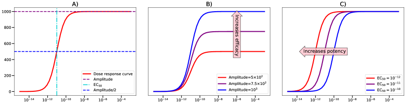
Figure 1: Sigmoid dose-response curve: number of signalling complexes formed, $\sigma(L)$, as a function of the concentration of ligand $L$ (arbitrary units). A) The maximum value defines the amplitude. The EC₅₀ is the concentration of ligand which corresponds to half the amplitude. B) Three dose-response curves with the same EC₅₀ value and different amplitudes. Increasing the amplitude shifts up the maximum of the curve and increases the efficacy. C) Three dose-response curves with the same amplitude and different EC₅₀ values. Decreasing the EC₅₀ shifts the dose-response curve to the left and increases the potency of the ligand.

Definition 2.10.

We define the signalling function, $\sigma:\mathbb{R}_{+}\to\mathbb{R}_{+},\,L\mapsto\sigma(L)$, as the univariate function which assigns to a given value of ligand concentration, $L$, the number (or concentration) of signalling complexes formed at steady state. The dose-response curve is the corresponding plot of the signalling function.

We note that in what follows we will not distinguish between number (or concentration) of signalling complexes since one can be obtained from the other if we know the volume of the system and Avogadro’s number.

The specific choice of $\sigma$ will depend on the receptor-ligand system under consideration. In this paper we focus on the class of cytokine receptors and the signalling function will be defined in Section 3. In our examples the signalling function will be a product of the steady state values (numbers) of sub-unit chains that make up the full receptor, intra-cellular kinases, affinity constants of the reactions involved, and ligand concentration. This together with equations (2) and (3) indicate that the signalling function will always be algebraic. Next, we define a central object of study in this paper; namely, the amplitude of the signalling function, often referred as efficacy in the pharmacology literature [3].

Definition 2.11.

The amplitude of the signalling function, $A$, is the difference between the maximum and the minimum of $\sigma$; that is, $A\equiv max(\sigma)-min(\sigma)$.

We note that when $\min(\sigma)=0$, which is the case considered in this paper ($\min(\sigma)=\sigma(0)=0$), the amplitude is given by the maximum of the signalling function. If, in addition, the dose-response curve attains its maximum at large concentrations (for instance, when the dose-response curve is sigmoid), we have

$$A=\lim_{L\to+\infty}\sigma(L).$$ (4)

The amplitude provides information about the magnitude of the intra-cellular response to the stimulus, $L$. The larger the amplitude is, the larger the response variability will be. The amplitude is always bounded by the number of molecules available. However, this bound is often not tight [45]. To quantify the sensitivity of the model to the stimulus, i.e., the potency of the ligand $L$, we introduce the half-maximal effective concentration, EC₅₀.

Definition 2.12.

The half-maximal effective concentration, or EC₅₀, is the ligand concentration $L^{*}$ which satisfies $\sigma(L^{*})=min(\sigma)+\frac{max(\sigma)-min(\sigma)}{2}=min(\sigma)+\frac{A}{2}$.

We say that the EC₅₀ is inversely proportional to ligand potency; namely, the lower the EC₅₀, the higher the potency of the ligand. Figure 1 illustrates the amplitude and the EC₅₀ of a sigmoid dose-response curve (A) when its minimum is zero: increasing the amplitude shifts up the maximum of the curve and results in greater efficacy (B), and decreasing the EC₅₀ shifts the dose-response curve to the left and increases the potency of the ligand (C). We now review some algebraic and analytic tools which will enable us to compute the EC₅₀ and the amplitude.

2.3 Gröbner bases

Since we assume the law of mass action, the models studied in this paper are systems of polynomial equations, and thus, we can use the techniques developed in the field of computational algebra and algebraic geometry [46]. Such methods have also been successfully applied to many topics in chemical reaction network theory, see e.g., Refs. [47, 48, 49]. In particular, we make use of Gröbner bases. Informally speaking, a Gröbner basis is a non-linear generalisation of the concept of a basis in linear algebra and, therefore when a Gröbner basis for a polynomial system is calculated, many properties of the system can be investigated, such as the number of solutions and the dimensionality of the space of solutions. Strictly speaking, however, a Gröbner basis is not a basis as it is not unique and it depends on the lexicographical (lex) monomial ordering chosen. For more details we refer the reader to Ref. [46].

A lex Gröbner basis is a triangular polynomial system; that is, for a polynomial system (ideal) in $\mathbb{Q}[x_{1},\ldots,x_{n}]$ we obtain a polynomial system of the form

$$g_{n}(x_{1},\ldots,x_{n})=g_{n-1}(x_{1},\ldots,x_{n-1})=\dots=g_{1}(x_{1})=0.$$ (5)

We note that when the solution space is positive dimensional, then $g_{1},\ldots,g_{n}$ are identically zero. For a given Gröbner basis with zero-dimensional solution space we can now iteratively, and often numerically, solve the constituent polynomials to obtain the solutions (in $\mathbb{C}^{n}$) for the polynomial system. We can also find all real and, further, positive solutions, if there are any [46].

3 Methods: analytical study of receptor-ligand systems

In this section we first outline the computation of the analytic expressions of the steady state, amplitude and EC₅₀ for two IL-7 receptor (IL-7R) models. These two examples then allow us to introduce a more general method to analytically compute the amplitude and the EC₅₀ of receptor-ligand systems under the following hypotheses:

1. The system is in steady state.

2. The ligand is in excess (we consider ligand concentration, $L$, as a parameter instead of a dynamic variable).

3. A unique biologically relevant solution exists for any given set of rate constants and initial conditions.

The IL-7R models we have chosen are simple enough to illustrate our method, and thus, to derive analytic expressions for the amplitude and the EC₅₀, yet complex enough to show its limitations.

3.1 Two motivating examples: IL-7 cytokine receptor as a paradigm

We now consider the cytokine interleukin-7 (IL-7) and its receptor (IL-7R) [50, 9, 8, 10, 15, 12] as a motivating receptor-ligand system. IL-7 is a cytokine involved in T cell development, survival and homeostasis [51]. Its receptor, IL-7R, is displayed on the surface of T cells and is composed of two trans-membrane chains: the common gamma chain (denoted by $\gamma$) and the specific high affinity chain IL-7R$\alpha$ (denoted by $\alpha$) [8, 12, 51, 13]. Cytokine receptors do not contain intrinsic kinase domains, and thus, make use of Janus family tyrosine kinases (JAKs) and signal in part by the activation of signal transducer and activator of transcription (STAT) proteins [52]. In the case of the gamma chain, it binds to the intra-cellular extrinsic Janus kinase molecule, JAK3. Binding of IL-7 to the dimeric JAK3-bound IL-7 receptor, defined as $\alpha:\gamma:JAK3$, initiates a series of biochemical reactions from the membrane of the cell to its nucleus, which in turn lead to a cellular response. For the IL-7R system the STAT protein preferentially activated is STAT5 [52], so that the amount of phosphorylated STAT5 can be used as the experimental measure of the intra-cellular response generated by the IL-7 stimulus. The IL-7R receptor is illustrated in Figure 2(a), where the hatched area determines the intra-cellular environment.

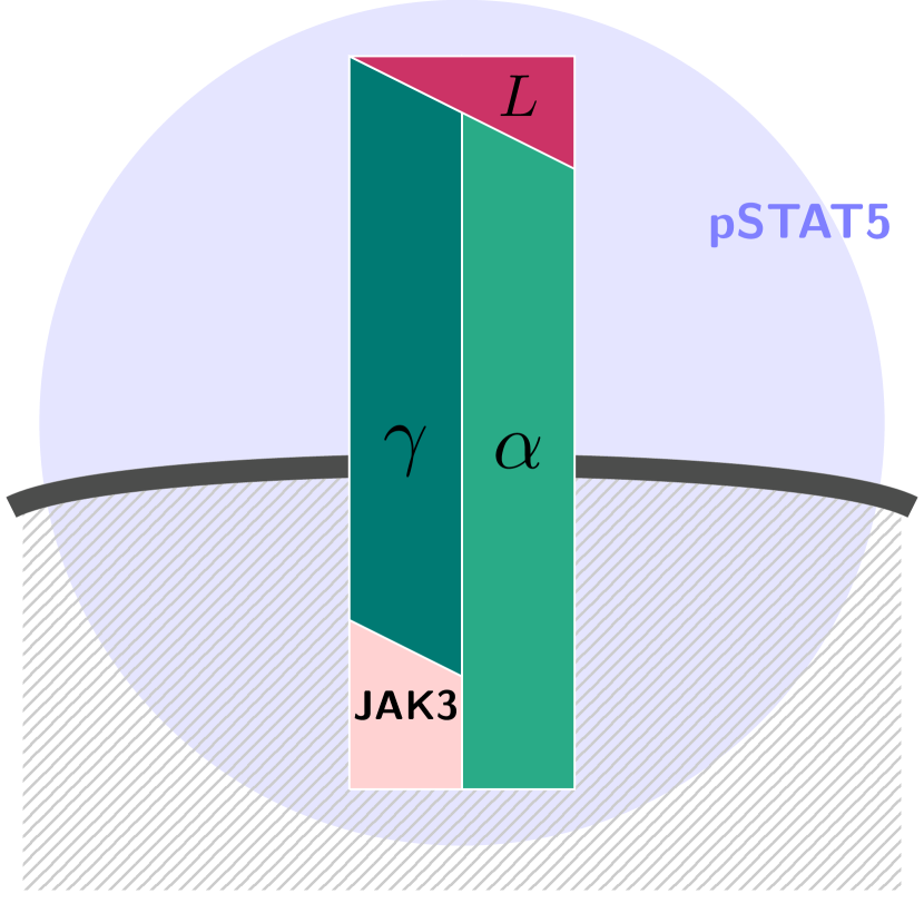
(a) Signalling IL-7 complex.

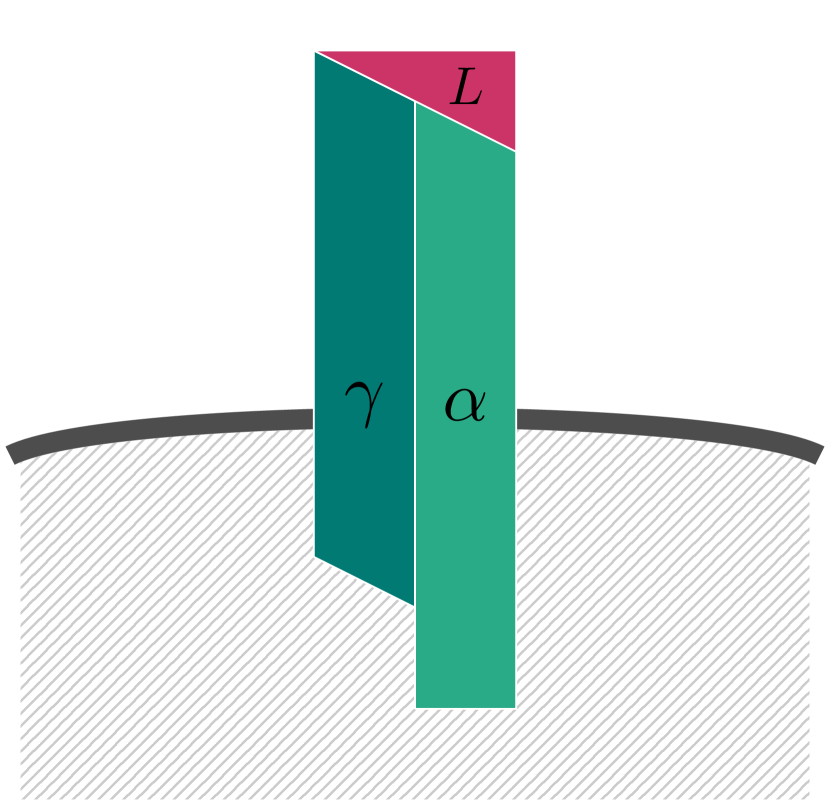
(b) Dummy IL-7 complex.

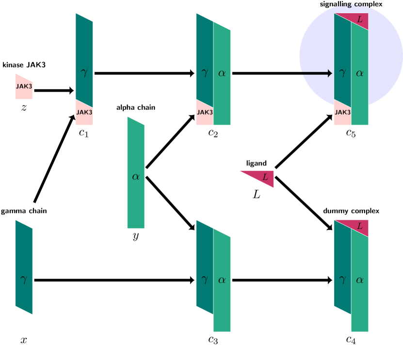
(c) IL-7R model: sequential chemical reaction scheme.

Figure 2: First IL-7R model: (a) The IL-7 receptor is composed of the trans-membrane $\gamma$ and $\alpha$ chains. The $\gamma$ chain can bind the intra-cellular downstream kinase JAK3. When the ligand, IL-7, binds the full receptor, it phosphorylates STAT5. (b) The IL-7R model allows the formation of ‘‘dummy’’ complexes: IL-7 bound IL-7R complexes, devoid of JAK3, which are unable to induce intra-cellular signalling. (c) IL-7 bound IL-7R complexes with JAK3 are able to induce intra-cellular signalling, and thus, are called ‘‘signalling’’ complexes. IL-7R dummy and signalling complexes are formed sequentially. The mathematical notation used in this paper is shown below each molecule or complex.

The first model we consider is shown in Figure 2(c). As discussed in Ref. [9], the gamma chain is shared by other cytokine receptors. This model does not include the competition for the gamma chain between different cytokine receptors, therefore later in this section we introduce a second model to account for this competition. In this section we will provide an (algebraic) analytic treatment of both models. We consider the formation of ‘‘dummy’’ receptors, $\alpha:\gamma$, which are formed of the IL-7R devoid of JAK3 and, therefore, they cannot signal (see Figure 2(b)). We further assume no allostery; that is, the affinity constants of the biochemical reactions involved in the formation of the dummy complex, $L:\alpha:\gamma$, are the same as the affinity constants involved in the formation of the signalling complex, $L:\alpha:\gamma:JAK3$.

3.1.1 The IL-7 receptor-ligand system: two receptor chains and a kinase

We first consider a model in which the IL-7R is formed sequentially, one molecule at a time; the $\gamma$ chain binds to the kinase, JAK3, then the $\alpha$ chain binds to the complex formed by $\gamma$ and JAK3. Finally, the ligand, IL-7, binds to the signalling receptor composed of $\gamma$, $\alpha$ and $JAK3$. The model also includes the formation of ‘‘dummy’’ receptors, which do not involve the kinase JAK3. Figure 2(c) illustrates the sequential formation of the signalling and dummy complexes. The reaction scheme for this model is as follows

$$\begin{array}[]{lllccl}\gamma+JAK3&\rightleftharpoons&\gamma:JAK3,&&&K_{1},\\ \alpha+\gamma:JAK3&\rightleftharpoons&\alpha:\gamma:JAK3,&&&K_{2},\\ \alpha+\gamma&\rightleftharpoons&\alpha:\gamma,&&&K_{2},\\ L+\alpha:\gamma&\rightleftharpoons&L:\alpha:\gamma,&&&K_{3},\\ L+\alpha:\gamma:JAK3&\rightleftharpoons&L:\alpha:\gamma:JAK3,&&&K_{3},\\ \end{array}$$ (6)

where for $i=1,2,3$, $K_{i}$ is the affinity constant of the appropriate reaction. One can show that this system has deficiency zero and is reversible (see Section 2.1). Therefore, for every set of rate constants and initial conditions, there exists exactly one positive steady state. Moreover, this positive steady state is in detailed balance. We remind the reader that in this paper we assume mass action kinetics to determine reaction rates. We denote the concentration of $\gamma$, $\alpha$, JAK3 and IL-7 by $x$, $y$, $z$, and $L$, respectively. The reaction rate for the forward/backward reaction ($\rightharpoonup$/$\leftharpoondown$) is given by $k_{i}$ and $q_{i}$, respectively, for $i=1,2,3$. We note that $K_{i}=k_{i}/q_{i}$. The concentrations of the product complexes of the forward reactions are denoted by $c_{i}$ in order of appearance (see Figure 2(c)). We can now write down the ordinary differential equations (ODEs) associated to the system of reactions (6):

$$\frac{dx}{dt} =-k_{1}xz+q_{1}c_{1}-k_{2}xy+q_{2}c_{3},$$ (7)

$$\frac{dy}{dt} =-k_{2}yc_{1}+q_{2}c_{2}-k_{2}xy+q_{2}c_{3},$$

$$\frac{dz}{dt} =-k_{1}xz+q_{1}c_{1},$$

$$\frac{dc_{1}}{dt} =k_{1}xz-q_{1}c_{1}-k_{2}yc_{1}+q_{2}c_{2},$$

$$\frac{dc_{2}}{dt} =k_{2}yc_{1}-q_{2}c_{2}-k_{3}c_{2}L+q_{3}c_{5},$$

$$\frac{dc_{3}}{dt} =k_{2}xy-q_{2}c_{3}-k_{3}c_{3}L+q_{3}c_{4},$$

$$\frac{dc_{4}}{dt} =k_{3}c_{3}L-q_{3}c_{4},$$

$$\frac{dc_{5}}{dt} =k_{3}c_{2}L-q_{3}c_{5}.$$

A suitable basis for the conservation equations is

$$N_{x} =x+c_{1}+c_{2}+c_{3}+c_{4}+c_{5},$$ (8)

$$N_{y} =y+c_{2}+c_{3}+c_{4}+c_{5},$$

$$N_{z} =z+c_{1}+c_{2}+c_{5};$$

that is, single chain molecules are conserved since we do not consider the generation or degradation of molecules. The constants $N_{x}$, $N_{y}$ and $N_{z}$ represent the total copy number of $\gamma$, $\alpha$ and JAK3 molecules per cell, respectively. Detailed balance leads to the following steady state equations:

$$c_{1} =K_{1}xz,$$ (9)

$$c_{2} =K_{2}yc_{1},$$

$$c_{3} =K_{2}xy,$$

$$c_{4} =K_{3}Lc_{3},$$

$$c_{5} =K_{3}Lc_{2}.$$

Substituting the steady state equations into the conservation equations, we obtain a system of polynomials

$$0 =-N_{x}+x+K_{1}xz+K_{2}K_{1}xyz+K_{2}xy+K_{3}K_{2}Lxy+K_{3}K_{2}K_{1}Lxyz,$$ (10)

$$0 =-N_{y}+y+K_{2}K_{1}xyz+K_{2}xy+K_{3}K_{2}Lxy+K_{3}K_{2}K_{1}Lxyz,$$

$$0 =-N_{z}+z+K_{1}xz+K_{2}K_{1}xyz+K_{3}K_{2}K_{1}Lxyz.$$

Analytic computation of the steady state.

The polynomial system (10) can be solved numerically for a particular set of parameter values. However, an analytic solution will provide greater insight and will allow us to derive expressions for the amplitude and the EC₅₀. We make use of Macaulay2 [53] to compute a lex Gröbner basis for this model, which will lead to a triangular set of polynomials , as follows:

$$0 =z^{2}+\frac{[1+K_{1}(N_{x}-N_{z})]}{K_{1}}z-\frac{N_{z}}{K_{1}},$$ (11a)

$$0 =y^{2}+\frac{[1+K_{2}(K_{3}L+1)(N_{x}-N_{y})]}{K_{2}(K_{3}L+1)}y-\frac{N_{y}}{K_{2}(K_{3}L+1)},$$ (11b)

$$0 =x-\frac{1}{N_{x}}yz-\frac{(N_{x}-N_{z})}{N_{x}}y-\frac{(N_{x}-N_{y})}{N_{x}}z-\frac{N_{x}(N_{x}-N_{y}-N_{z})+N_{y}N_{z}}{N_{x}}.$$ (11c)

Equation (11c) gives

$$x=\frac{(N_{x}-N_{y}+y)(N_{x}-N_{z}+z)}{N_{x}}=\frac{N_{x}-N_{y}+y}{1+K_{1}z},$$

where the last equality follows from equation (11a). Solving the system (11) and selecting the biologically relevant solution, we obtain an analytic expression for the number of free (unbound) JAK3, $\alpha$ and $\gamma$ molecules at steady state

$$z =\frac{-1+K_{1}(N_{z}-N_{x})+\sqrt{\Delta_{1}}}{2K_{1}},$$ (12a)

$$y =\frac{-1+K_{2}(N_{y}-N_{x})(K_{3}L+1)+\sqrt{\Delta_{2}}}{2K_{2}(K_{3}L+1)},$$ (12b)

$$x =\frac{N_{x}-N_{y}+y}{1+K_{1}z},$$ (12c)

where we have introduced

$$\Delta_{1} =4K_{1}N_{z}+\left[K_{1}(N_{x}-N_{z})+1\right]^{2},$$

and

$$\Delta_{2} =4K_{2}N_{y}\left(K_{3}L+1\right)+\left[K_{2}(N_{x}-N_{y})(K_{3}L+1)+1\right]^{2}.$$

We study the dose-response curve of this model given by the number of signalling complexes, $L:\gamma:\alpha:JAK$, per cell at steady state and as a function of $L$. The signalling function, $\sigma(L)$, is given by

$$\sigma(L)\equiv c_{5}=K_{3}K_{2}K_{1}Lxyz.$$ (13)

.

Analytic computation of the amplitude.

A simple inspection of the behaviour of (12) shows that the dose-response curve is a sigmoid, such that $\sigma(0)=0$. Therefore the amplitude $A$ is given by the asymptotic behaviour of the signalling function as follows:

$$A\equiv\lim_{L\to+\infty}\sigma(L).$$ (14)

We will prove this result rigorously for a more general class of models in Section 4.

We first notice that $z$ is independent of $L$. We now compute the product $xy$ (at steady state) as follows

$$xy=\frac{(N_{x}-N_{y})y+y^{2}}{1+K_{1}z}.$$

From equation (11b) we can replace the polynomial in $y$ of degree two by an expression linear in $y$:

$$(N_{x}-N_{y})y+y^{2}=\frac{N_{y}-y}{K_{2}(K_{3}L+1)}.$$

Thus, we obtain the following analytic expression for the signalling function:

$$\sigma(L)=K_{3}K_{2}K_{1}Lxyz=\frac{K_{1}z}{(1+K_{1}z)}\frac{K_{3}L}{(K_{3}L+1)}(N_{y}-y).$$ (15)

Since $\frac{K_{3}L}{1+K_{3}L}\to 1$ when $L\to+\infty$, we need to study the expression $N_{y}-y$ in this limit. We have

$$N_{y}-y=\frac{(N_{y}+N_{x})K_{2}(K_{3}L+1)+1-\sqrt{\Delta_{2}}}{2K_{2}(K_{3}L+1)},$$ (16)

where

$$\Delta_{2}=K_{2}^{2}(K_{3}L+1)^{2}(N_{x}-N_{y})^{2}+2K_{2}(K_{3}L+1)(N_{x}+N_{y})+1.$$

Keeping to lowest order in $\mathcal{O}(\frac{1}{L})$ we obtain

$$N_{y}-y =\frac{1+(N_{x}+N_{y})K_{2}(K_{3}L+1)-K_{2}(K_{3}L+1)|N_{x}-N_{y}|(1+\mathcal{O}(\frac{1}{L}))}{2K_{2}(K_{3}L+1)},$$ (17)

$$=\frac{N_{x}+N_{y}-|N_{x}-N_{y}|}{2}+\mathcal{O}(\frac{1}{L}).$$ (18)

Finally, noticing that

$$\frac{N_{x}+N_{y}-|N_{x}-N_{y}|}{2}=\text{min}(N_{x},N_{y}),$$

we obtain the amplitude

$$A=\text{min}(N_{x},N_{y})\frac{K_{1}z}{1+K_{1}z},$$ (19)

where $z$ is the analytic expression obtained in (12). This result indicates that the amplitude of this model is the total number of the limiting trans-membrane chain modulated by a factor, valued in the interval $[0,1]$, which only depends on $K_{1}$, $N_{x}$ and $N_{z}$.

Analytic computation of the EC₅₀.

We now determine the EC₅₀ by finding the value of $L_{50}$ such that

$$\sigma(L_{50})=\frac{A}{2}=K_{1}K_{2}K_{3}L_{50}x_{50}y_{50}z_{50},$$ (20)

where $x_{50}$, $y_{50}$ and $z_{50}$ are the steady state expressions found in (12) evaluated at $L=L_{50}$. Two expressions satisfy this equation but only one provides a relevant biological solution with $L,x,y,z>0$. The relevant analytic expression of the EC₅₀ is given by

$$EC_{50}=M\;\frac{1+K_{2}(N_{x}+N_{y}-M)+\sqrt{1+K_{2}^{2}(N_{y}-N_{x})^{2}+2K_{2}(N_{x}+N_{y}-M)}}{K_{2}K_{3}(M-2N_{x})(M-2N_{y})},$$ (21)

with $M=\text{min}(N_{x},N_{y})$. The details of the computation can be found in Appendix B. This result shows that the EC₅₀ value for this system is independent of the kinase, since the parameters $K_{1}$ and $N_{z}$ are absent in the previous expression.

Alternatively, we now propose a more algebraic method to derive the analytic expression of the EC₅₀. We compute a lex Gröbner basis for the augmented system of polynomials consisting of the steady state equations (10) and

$$K_{1}K_{2}K_{3}Lxyz\;(1+K_{1}z)-\frac{MK_{1}z}{2}=0,$$ (22)

where this time $x$, $y$, $z$, and $L$ are variables. The resulting triangular system describes directly the EC₅₀ and $x$, $y$, $z$ at $L=$EC₅₀:

$$0 =L^{2}+\frac{2M[-1+K_{2}(M-N_{x}-N_{y})]}{K_{2}K_{3}(M-2N_{x})(M-2N_{y})}L+\frac{M^{2}}{K_{3}^{2}(M-2N_{x})(M-2N_{y})},$$ (23a)

$$0 =z^{2}+\frac{1+K_{1}(N_{x}-N_{z})}{K_{1}}z-\frac{N_{z}}{K_{1}},$$ (23b)

$$0 =y-\frac{K_{3}(M-2N_{x})(M-2N_{y})}{2M}L+\frac{K_{2}(2N_{x}-M)+2}{2K_{2}},$$ (23c)

$$0 =x-\frac{K_{3}(M-2N_{x})(M-2N_{y})(N_{x}-N_{z}+z)}{2MN_{x}}L+\frac{[2+K_{2}(2N_{y}-M)](N_{x}-N_{z}+z)}{2K_{2}N_{x}}.$$ (23d)

Solving (23a) and selecting the solution for which $y$ and $x$, given by equations (23c) and (23d), respectively, are positive yields the final result, in agreement with (21).

3.1.2 The IL-7 receptor-ligand system: an additional sub-unit receptor chain

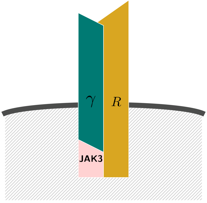
(a) Decoy complex with kinase.

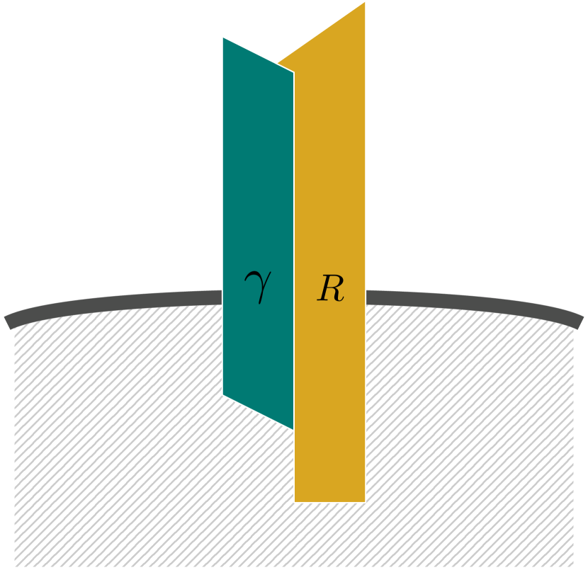
(b) Decoy complex without kinase.

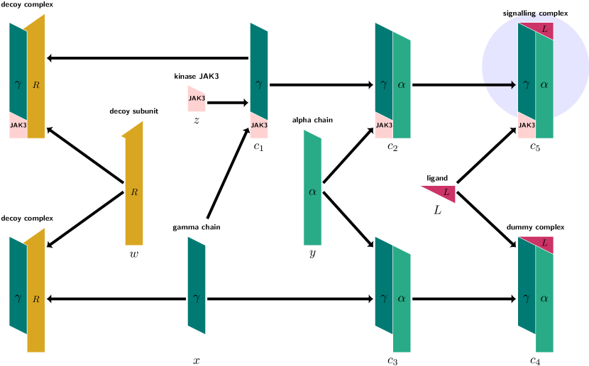
(c) Second IL-7R model: sequential chemical reaction scheme.

Figure 3: IL-7R model with an additional receptor sub-unit. The signalling and dummy complexes are the same as in the first IL-7R model. This second model allows the formation of decoy complexes: (a) with the kinase JAK3, or (b) without the kinase. (c) The IL-7R dummy and signalling complexes are formed sequentially. Decoy complexes can be formed to prevent the formation of signalling or dummy complexes. The mathematical notation used is annotated below each molecule or complex.

The previous model described the IL-7 receptor system without any consideration for the fact that the $\gamma$ chain is shared with other cytokine receptors [9]. We now account for this competition by including in the previous model an additional receptor chain, $R$, which can bind to the $\gamma$ chain, or the complex $\gamma:JAK3$, to form decoy receptor complexes (see Figure 3(a) and Figure 3(b), where the hatched area indicates the cytoplasmic region). The resulting reaction scheme (summarised in Figure 3(c)) is given by

$$\begin{array}[]{lllccl}JAK3+\gamma&\rightleftharpoons&JAK3:\gamma&&&K_{1},\\ \alpha+JAK3:\gamma&\rightleftharpoons&\alpha:\gamma:JAK3&&&K_{2},\\ \alpha+\gamma&\rightleftharpoons&\alpha:\gamma&&&K_{2},\\ L+\alpha:\gamma&\rightleftharpoons&L:\alpha:\gamma&&&K_{3},\\ L+\alpha:\gamma:JAK3&\rightleftharpoons&L:\alpha:\gamma:JAK3&&&K_{3},\\ R+\gamma&\rightleftharpoons&R:\gamma&&&K_{4},\\ R+JAK3:\gamma&\rightleftharpoons&R:\gamma:JAK3&&&K_{4}.\end{array}$$

We use $w$ to describe the concentration of the additional chain $R$. Similarly to the previous model, we write the system of ODEs describing the time evolution for each complex and then derive (a basis for) the conservation and steady state equations. Combining them, we obtain the following polynomial system:

$$0 =-N_{x}+x+K_{2}xy+K_{1}xz+K_{2}K_{1}xyz+K_{3}K_{2}Lxy+K_{3}K_{2}K_{1}Lxyz+K_{4}xw+K_{1}K_{4}xwz,$$ (24)

$$0 =-N_{y}+y+K_{2}xy+K_{2}K_{1}xyz+K_{3}K_{2}Lxy+K_{3}K_{2}K_{1}Lxyz,$$

$$0 =-N_{z}+z+K_{1}xz+K_{2}K_{1}xyz+K_{3}K_{2}K_{1}Lxyz+K_{1}K_{4}xwz,$$

$$0 =-N_{w}+w+K_{4}xw+K_{4}K_{1}xwz,$$

where $N_{w}$ is the additional conserved quantity. Again, we compute a lex Gröbner basis for this set of polynomials to obtain the following triangular system:

$$0 =K_{1}z^{2}+z[1+K_{1}(N_{x}-N_{z})]-N_{z},$$ (25a)

$$0 =Ay^{3}+By^{2}+Cy+D,$$ (25b)

$$0 =\left[K_{2}K_{4}(1+K_{3}L)N_{x}N_{y}\right]x+(Ay^{2}+By+C+K_{4}N_{y})(N_{x}-N_{z}+z),$$ (25c)

$$0 =\left[K_{2}K_{4}(1+K_{3}L)N_{y}\right]w+Ay^{2}+By+[K_{2}(1+K_{3}L)-K_{4}]N_{y},$$ (25d)

where

$$A =-K_{2}(1+K_{3}L)[K_{2}(1+K_{3}L)-K_{4}],$$

$$B =K_{4}-K_{2}(1+K_{3}L)[1+K_{4}(N_{w}-N_{x}+2N_{y})+K_{2}(1+K_{3}L)(N_{x}-N_{y})],$$

$$C =N_{y}[-2K_{4}+K_{2}(1+K_{3}L)(1+K_{4}(N_{w}-N_{x}+N_{y}))],$$

$$D =K_{4}N_{y}^{2}.$$

Solving (25a) gives the number of free JAK3 molecules per cell at steady state, $z$; solving (25b) gives the number of free (unbound) $\alpha$ chains per cell, $y$; and substituting $y$ and $z$ into (25c) and (25d) gives the remaining steady states. We obtain the following implicit steady state expressions for the number of free (unbound) chains:

$$z= \frac{-1+K_{1}(N_{z}-N_{x})+\sqrt{[1+K_{1}(N_{x}-N_{z})]^{2}+4N_{z}K_{1}}}{2K_{1}},$$ (26)

$$x= -\frac{(Ay^{2}+By+C+K_{4}N_{y})(N_{x}-N_{z}+z)}{K_{2}K_{4}(1+K_{3}L)N_{x}N_{y}},$$

$$w= -\frac{Ay^{2}+By+[K_{2}(1+K_{3}L)-K_{4}]N_{y}}{K_{2}K_{4}(1+K_{3}L)N_{y}}.$$

The problem now reduces to finding the positive real roots of (25b). As (25b) is a polynomial of degree three, we could, in principle, find an exact analytic solution. However, such a solution might not be very informative. Instead, we show how perturbation theory can be used to obtain the amplitude of the dose-response. In this model, the signalling complex is still $L:\alpha:\gamma:JAK3$. The signalling function is given by

$$\sigma(L)\equiv K_{3}K_{2}K_{1}Lxyz.$$ (27)

In Section 4.3 we will show that, for this model, the maximum of $\sigma$ is attained in the limit $L\to+\infty$. Hence, we have

$$A\equiv\lim_{L\to+\infty}\sigma(L).$$ (28)

Combining (25a), written as $N_{x}-N_{z}+z=\frac{N_{x}}{1+K_{1}z}$, and (25b), we obtain a reduced expression for the product $xy$

$$xy=\frac{N_{y}-y}{K_{2}(1+K_{3}L)(1+K_{1}z)},$$ (29)

which allows us to rewrite the amplitude as

$$A=\lim_{L\to+\infty}\frac{K_{1}z}{(1+K_{1}z)}\frac{K_{3}L}{(K_{3}L+1)}(N_{y}-y).$$ (30)

We note that $z$ is independent of $L$ and, therefore, to compute the amplitude we only need to find the behaviour of $y$ as $L\to+\infty$.

Perturbation theory to determine $y$ as $L\to+\infty$.

We now apply the method described in Ref. [54] and summarised in Appendix A. Let $\epsilon=\tfrac{1}{L}$ and define the polynomial $P_{\epsilon}$ as follows:

$$P_{\epsilon}(y)\equiv P_{2}(y)\epsilon^{2},$$

where $P_{2}$ is the polynomial (25b). We added a factor of $\epsilon^{2}$ to remove any negative powers of $\epsilon$ in $P_{2}$. We obtain the polynomial

$$P_{\epsilon}(y)=A_{\epsilon}y^{3}+B_{\epsilon}y^{2}+C_{\epsilon}y+D_{\epsilon},$$ (31)

where

$$A_{\epsilon}= -K_{2}(\epsilon+K_{4})[K_{2}(\epsilon+K_{4})-\epsilon K_{6}],$$

$$B_{\epsilon}= K_{2}^{2}K_{4}^{2}(N_{y}-N_{x})-\epsilon K_{2}K_{4}[1+2K_{2}N_{x}-2K_{2}N_{y}+K6(N_{w}-N_{x}+2N_{y})]$$

$$+ \epsilon^{2}(K_{6}-K_{2}(1+K_{2}N_{x}-K_{2}N_{y}+K_{6}(N_{w}-N_{x}+2N_{y}))),$$

$$C_{\epsilon}= \epsilon N_{y}(K_{2}K_{4}(1+K_{6}(N_{w}-N_{x}+N_{y}))+\epsilon(K_{2}-2K_{6}+K_{2}K_{6}(N_{w}-N_{x}+N_{y}))),$$

$$D_{\epsilon}= K_{6}N_{y}^{2}\epsilon^{2}.$$

We now replace $y$ by $\epsilon^{p}\omega(\epsilon)$ with $\omega(0)\neq 0$ according to theorem A.3. We obtain

$$P_{\epsilon}(\epsilon^{p}\omega(\epsilon))=A_{p,\epsilon}\omega^{3}+B_{p,\epsilon}\omega^{2}+C_{p,\epsilon}\omega+D_{p,\epsilon},$$ (32)

where

$$A_{p,\epsilon}= -\epsilon^{3p}K_{2}(\epsilon+K_{4})(K_{2}(\epsilon+K_{4})-\epsilon K_{6}),$$

$$B_{p,\epsilon}= \epsilon^{2p}(K_{2}^{2}K_{4}^{2}(N_{y}-N_{x})-\epsilon K_{2}K_{4}(1+2K_{2}(N_{x}-N_{y})+K_{6}(N_{w}-N_{x}+2N_{y}))$$

$$+ \epsilon^{2}(K_{6}-K_{2}(1+K_{2}N_{x}-K_{2}N_{y}+K_{6}(N_{w}-N_{x}+2N_{y})))),$$

$$C_{p,\epsilon}= \epsilon^{1+p}N_{y}(K_{2}K_{4}(1+K_{6}(N_{w}-N_{x}+N_{y}))+\epsilon(K_{2}-2K_{6}+K_{2}K_{6}(N_{w}-N_{x}+N_{y}))),$$

$$D_{p,\epsilon}= K_{6}N_{y}^{2}\epsilon^{2}.$$

The smallest exponents in the previous equation are

$$E=\{2,1+p,2p,3p\}.$$

We note that $0$ is not in $E$ because we multiplied $P_{2}$ by $\epsilon^{2}$. Applying the graphical algorithm detailed in Appendix A, we find the proper values $(0,0)$ and $(1,2)$ (see Figure 4). We investigate these two branches.

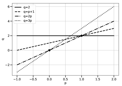
Figure 4: The lines defined in set $E$ and the proper values, (black dots), computed following the graphical algorithm described in Appendix A.

Branch (0,0).

We make use of the notation in Appendix A, to define

$$T_{\epsilon}^{(1)}(\omega)\equiv\epsilon^{0}P_{\epsilon}(\omega\epsilon^{0}).$$

The least common denominator of {2,1,0,0} is $q_{1}=1$. Therefore in accordance with the notation of Appendix A

$$\epsilon=\beta,$$

and the polynomial $R_{\beta}^{(1)}$ defined as

$$R_{\beta}^{(1)}(\omega)\equiv T_{\epsilon}^{(1)}(\omega),$$

is the polynomial $P_{\epsilon}$. It means that we have $y=\omega$ and we can directly carry out a regular perturbation expansion.

Let us write the asymptotic expansion $y=y_{0}+y_{1}\epsilon+y_{2}\epsilon^{2}+\ldots$ and replace it in $P_{\epsilon}(y)$. Since $P_{\epsilon}(y)=0$, by the fundamental theorem of perturbation theory (Theorem A.2) we obtain a system of equations in $y_{0}$, $y_{1},\ldots$, which can be solved. The first equation of the system is given by

$$-K_{2}^{2}K_{3}^{2}y_{0}^{2}(N_{x}-N_{y}+y_{0})=0.$$ (33)

We are are only interested in non-negative values of $y_{0}$, since we want $y$ to be biologically relevant. We also require $\omega(0)=y(0)=y_{0}\neq 0$ from Theorem A.3. Thus, solving equation (33), we obtain $y_{0}=N_{y}-N_{x}$ if $N_{y}>N_{x}$ and $y_{0}=0$ otherwise. Assuming $y_{0}=0$ (i.e., $N_{x}\geq N_{y}$), we solve the next order equation

$$K_{4}N_{y}^{2}+K_{2}K_{3}N_{y}(1+K_{4}(N_{w}-N_{x}+N_{y}))y_{1}+K_{2}^{2}K_{3}^{2}(N_{y}-N_{x})y_{1}^{2}=0.$$ (34)

We select the positive root of this polynomial and obtain an expression for $y_{1}$ when $y_{0}=0$. Thus, we have

$$y_{1}=N_{y}\frac{1+K_{4}(N_{w}-N_{x}+N_{y})+\sqrt{1+2K_{4}(N_{w}+N_{x}-N_{y})+K_{4}^{2}(N_{w}-N_{x}+N_{y})^{2}}}{2K_{2}K_{3}(N_{x}-N_{y})}.$$ (35)

Equation (35) shows that $y_{1}>0$ when $N_{x}\geq N_{y}$. Hence, $y\approx\epsilon y_{1}$ converges to zero from above and, therefore, represents a biologically relevant solution. We can conclude that

$$\lim_{\epsilon\to 0}(N_{y}-y)=\left\{\begin{array}[]{ll}N_{x},&\text{if $N_{y}>N_{x}$,}\\ N_{y},&\text{otherwise.}\end{array}\right\}=\min(N_{x},N_{y}).$$ (36)

Branch (1,2).

On this branch, and again following the notation of Appendix 47, we define

$$T_{\epsilon}^{(2)}(\omega)\equiv\epsilon^{-2}P_{\epsilon}(\epsilon^{1}\omega).$$

The least common denominator of {2,1+1,0+1,0+1} is $q_{2}=1$, so $R_{\beta}^{(2)}$ is the same polynomial as $T^{(2)}_{\epsilon}$. Since $y=\omega\epsilon$, we have $N_{y}-y\underset{\epsilon\to 0}{\sim}N_{y}$. Furthermore, when replacing $\omega$ by an asymptotic expansion $\omega_{0}+\omega_{1}\epsilon+\ldots$ in $T_{\epsilon}^{(2)}$ and applying the fundamental theorem of perturbation theory (Theorem A.2), we obtain the same equation for $w_{0}$ as for $y_{1}$ in the previous branch (see equation (34)):

$$K_{4}N_{y}^{2}+K_{2}K_{3}N_{y}(1+K_{4}(N_{w}-N_{x}+N_{y}))\omega_{0}+K_{2}^{2}K_{3}^{2}(N_{y}-N_{x})\omega_{0}^{2}=0\;.$$ (37)

We have $y_{1}=\omega_{0}$. In other words, at large, but finite $L=1/\epsilon$, the convergence behaviour of the two branches is identical. This agrees with Theorem 2.7 which states that there is only one positive solution for each set of reaction constants and initial conditions. In conclusion, we find that $N_{y}-y=\text{min}(N_{x},N_{y})$, which gives the following expression for the amplitude

$$A\equiv\frac{K_{1}z}{1+K_{1}z}\text{min}(N_{x},N_{y}),$$ (38)

with $z$ defined in (26). As the steady state concentration of JAK3, $z$, is the same in the IL-7R model with or without the extra chain $R$, the amplitude of both models has the exact same expression.

Computation of the EC₅₀.

Since we did not compute analytic expressions for each steady state concentration, the EC₅₀ expression has to be obtained by computing a Gröbner basis of the polynomial system (24) augmented by the polynomial

$$K_{3}K_{2}K_{1}Lxyz(1+K_{1}z)-\frac{K_{1}zM}{2}=0,$$ (39)

considering $x,y,z$ and $L$ as variables, with $M=\text{min}(N_{x},N_{y})$. The lex Gröbner basis obtained for this system is:

$$0 =K_{1}z^{2}+(1+K_{1}(N_{x}-N_{z}))z-N_{z},$$ (40a)

$$0 =K_{3}aL^{3}+A_{L}L^{2}+B_{L}L+C_{L},$$ (40b)

$$0 =y+\frac{-aL^{2}+B_{y}L+C_{y}}{2K_{2}(K_{2}-K_{4})M^{2}},$$ (40c)

$$0 =w+\frac{aL^{2}+B_{w}L+C_{w}}{2K_{4}(K_{2}-K_{4})M^{2}},$$ (40d)

$$0 =x+\frac{aL^{2}+B_{x}L+C_{x}}{2K_{2}K_{4}M^{2}(1+K_{1}z)},$$ (40e)

where we wrote:

$$a =K_{2}^{2}K_{3}^{2}(M-2N_{x})(M-2N_{y})^{2},$$

$$A_{L} =K_{2}K_{3}^{2}M(M-2N_{y})(-2+3K_{2}M-K_{4}(M+2N_{w}-2N_{x})-2K_{2}(2N_{x}+N_{y})),$$

$$B_{L} =K_{3}M^{2}(2K_{4}+K_{2}(-2+3K_{2}M+2K_{4}(-M-N_{w}+N_{x}+N_{y})-2K_{2}(N_{x}+2N_{y}))),$$

$$C_{L} =K_{2}(K_{2}-K_{4})M^{3},$$

$$B_{y} =-\frac{A_{L}}{K_{3}},$$

$$C_{y} =M^{2}(-2K_{4}+K_{2}(2+K_{4}(M+2N_{w}-2N_{x})-2K_{2}(M-N_{x}-N_{y}))),$$

$$B_{w} =-2K_{2}K_{3}M(M-2N_{y})(1+K_{4}N_{w}+K_{2}(N_{x}+N_{y}-M)),$$

$$C_{w} =K_{2}M^{2}(K_{2}(M-2N_{y})-2K_{4}N_{w}),$$

$$B_{x} =-K_{2}K_{3}M(M-2N_{y})(2+K_{4}(M+2N_{w}-2N_{x})-2K_{2}(M-N_{x}-N_{y})),$$

$$C_{x} =M^{2}(2K_{4}+K_{2}(K_{2}-K_{4})(M-2N_{y})).$$

The polynomial (40a) is expected to be independent of the ligand concentration, $L$. The EC₅₀ expression is the real positive root of polynomial (40b) at which $x$, $y$ and $w$ (obtained via polynomials (40e), (40c) and (40d), respectively) are positive. The polynomial (40b) reflects the parameter dependency of the EC₅₀: since the parameters $K_{1}$ and $N_{z}$ are not present in its coefficients, we can affirm that the EC₅₀ is, once again, independent of the kinase. Thus, we reduced the problem of computing the EC₅₀ to solving a univariate polynomial (equation (40b)). In comparison, before any algebraic manipulation was possible, the polynomial system (24) had to be solved multiple times to obtain the dose-response curve (a sigmoid), which was then fitted with a Hill equation. Finally, the EC₅₀ was computed from the fitted parameters of the Hill curve. Alternatively, if one wanted to apply the Gröbner basis-free method of Section 3.1.1, one would have to solve the polynomial (25b) in $y$ (which is possible in theory), find its positive real solution (which is potentially hard), substitute the expression of $y$ into $\sigma(L)$, and then solve for the EC₅₀.

3.2 Summary of proposed algebraic method to study the signalling function

From the two previous examples, we devise a general algorithm to compute analytic expressions of the steady state, the amplitude and the EC₅₀ for some receptor-ligand systems when ligand is in excess.

Key steps 1) Write the mass action kinetics set of ODEs for the system under consideration. 2) Obtain the polynomial system by combining the steady state and conservation equations. 3) Compute a lex Gröbner basis of the polynomial system obtained in step 2. 4) Define the signalling function $\sigma(L)$. 5) Compute the amplitude expression by finding the extreme values of $\sigma$: $$\text{Amplitude}=\max(\sigma)-\min(\sigma).$$ 6) Compute a lex Gröbner basis of the polynomial system obtained in step 2 augmented by the equation $$\sigma(L)-\left[\frac{\text{Amplitude}}{2}+\min(\sigma)\right]=0,$$ with the ligand concentration, $L$, considered an additional variable. This additional equation corresponds to definition 2.12 of the EC₅₀. 7) Find the positive roots of the univariate polynomial in $L$ of the Gröbner basis obtained in step 6. The root which allows the other variables to be positive is the EC₅₀.

One of the crucial parts of the proposed algebraic algorithm is the amplitude computation. Usually, we have the simplification that $\min(\sigma)=\sigma(0)=0$, however, finding $\max(\sigma)$ can be challenging. For certain classes of models we have

$$\lim_{L\to+\infty}\sigma(L)=\text{max}(\sigma),$$

which greatly reduces the calculation. We can now either solve the Gröbner basis from step 3 directly, to obtain analytic expressions of the steady state concentrations of the single chains components, or use perturbation theory as outlined in Section 3.1.2. In the final step, if an exact expression for the EC₅₀ cannot be computed, i.e., the univariate polynomial in $L$ has a large degree, one already reduces the cost of the EC₅₀ computation compared to the naive approach. In summary, in this section we compute the lex Gröbner bases with the computer algebra package Macaulay2 [53] and provide a Macaulay2 code example in Appendix C.

4 Analytical study of general sequential receptor-ligand systems

In spite of the general applicability of the method outlined in the previous section, we still have to make the assumption that the computed limit of the signalling function coincides with its amplitude. In this section we show that this is indeed the case for a wider class of receptor-ligand systems. An analytic closed-form expression for the amplitude follows with little extra work. The EC₅₀ can then be studied making use of the extended Gröbner basis introduced in Section 3.2. We start by giving an abstract generalisation of the example from Section 3.1.1.

Definition 4.1 (SRLK model).

We call a sequential receptor-ligand model with extrinsic kinase (SRLK) a receptor-ligand model with the following properties:

• The receptor is composed of $n$ different trans-membrane chains, $X_{1},\ldots,X_{n}$, which bind sequentially,

  $$X_{1}:\ldots:X_{i-1}+X_{i}\rightleftharpoons X_{1}:\ldots:X_{i}\ \ \text{ for all }i\in\{2,\ldots,n\}.$$

• $X_{1}$ can bind reversibly to an intra-cellular extrinsic kinase $Z$.

• The signalling receptor is given by $Z:X_{1}:\ldots:X_{n}$ and the dummy receptor by $X_{1}:\ldots:X_{n}$.

• The extra-cellular ligand, $L$, binds reversibly to the signalling (or dummy) receptor, forming the signalling (or dummy) complex $Z:X_{1}:\ldots:X_{n}:L$ (or $X_{1}:\ldots:X_{n}:L$).

The biochemical reaction network for a general SRLK model is given by

$$\begin{array}[]{lllllccl}Z&+&X_{1}&\rightleftharpoons&Z:X_{1}&&&K_{0},\\ X_{2}&+&Z:X_{1}&\rightleftharpoons&Z:X_{1}:X_{2}&&&K_{1},\\ X_{2}&+&X_{1}&\rightleftharpoons&X_{1}:X_{2}&&&K_{1}^{\prime},\\ \vdots&&\vdots&&\vdots&&&\vdots\\ X_{i+1}&+&Z:X_{1}:\ldots:X_{i}&\rightleftharpoons&Z:X_{1}:\ldots:X_{i+1}&&&K_{i},\\ X_{i+1}&+&X_{1}:\ldots:X_{i}&\rightleftharpoons&X_{1}:\ldots:X_{i+1}&&&K_{i}^{\prime},\\ \vdots&&\vdots&&\vdots&&&\vdots\\ X_{n}&+&Z:X_{1}:\ldots:X_{n-1}&\rightleftharpoons&Z:X_{1}:\ldots:X_{n}&&&K_{n-1},\\ X_{n}&+&X_{1}:\ldots:X_{n-1}&\rightleftharpoons&X_{1}:\ldots:X_{n}&&&K_{n-1}^{\prime},\\ L&+&Z:X_{1}:\ldots:X_{n}&\rightleftharpoons&Z:X_{1}:\ldots:X_{n}:L&&&K_{n},\\ L&+&X_{1}:\ldots:X_{n}&\rightleftharpoons&X_{1}:\ldots:X_{n}:L&&&K_{n}^{\prime},\end{array}$$ (41)

where the $K_{i}$ (or $K_{i}^{\prime}$) are the affinity constants related to the formation of the signalling (or dummy) complex. Figure 5 illustrates the formation of the signalling and dummy complexes in an SRLK model with $n=4$ trans-membrane chains. We assume the system at steady state and that ligand is in excess. In what follows We refer to these two assumptions as the experimental hypotheses.

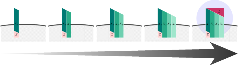
(a) Sequential formation of the signalling complex.

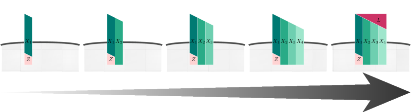
(b) Sequential formation of the dummy complex.

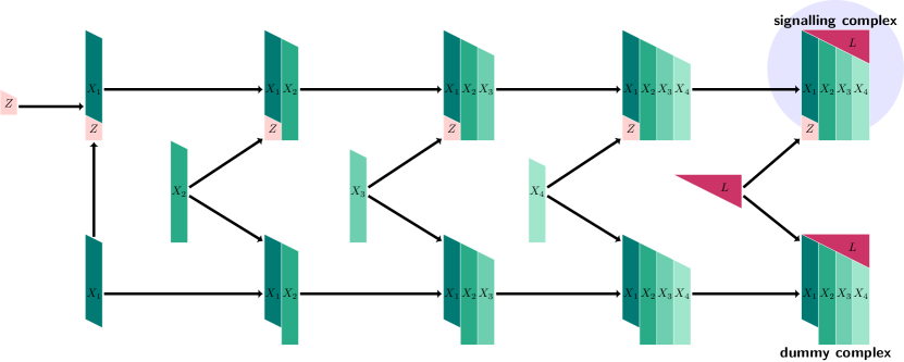
(c) SRLK model: sequential biochemical reaction scheme.

Figure 5: SRLK model with $n=4$ trans-membrane chains: (a)/(b) Sequential formation of the signalling/dummy complex. (c) Scheme of the sequential formation of the signalling/dummy complex: the chain $X_{1}$ binds first to the intra-cellular extrinsic kinase $Z$ (only for the signalling complex). Next, the chain $X_{2}$ binds to the complex $Z:X_{1}$ (or $X_{1}$) and $X_{3}$ binds to $Z:X_{1}:X_{2}$ (or $X_{1}:X_{2}$). Then, $X_{4}$ binds to $Z:X_{1}:X_{2}:X_{3}$ (or $X_{1}:X_{2}:X_{3}$). Finally, the ligand $L$ binds to the signalling receptor $Z:X_{1}:X_{2}:X_{3}:X_{4}$ (or dummy receptor $X_{1}:X_{2}:X_{3}:X_{4}$), thus forming the signalling (or dummy) complex.

We write $z$ (or $x_{i}$) for the steady state concentration of unbound chain $Z$ (or $X_{i}$). We also use $L$ to denote the ligand concentration. Finally, $N_{z}$ (or $N_{i}$) denotes the total copy number per cell of the species $Z$ (or $X_{i}$). An SRLK model satisfying the experimental hypotheses is then described by the following polynomial system:

$$N_{z} =z+K_{0}zx_{1}+K_{0}K_{1}zx_{1}x_{2}+\ldots+K_{0}K_{1}\ldots K_{n-1}zx_{1}\ldots x_{n}+K_{0}\ldots K_{n}zx_{1}\ldots x_{n}L$$ (42a)

$$=z+K_{0}z[x_{1}+\sum_{j=2}^{n}(\prod_{l=1}^{j-1}K_{l}x_{l}x_{j})+L\prod_{j=1}^{n}K_{j}x_{j}],$$

$$N_{1} =x_{1}+K_{1}^{\prime}x_{1}x_{2}+\ldots+K_{1}^{\prime}\ldots K_{n-1}^{\prime}x_{1}\ldots x_{n}+K_{1}^{\prime}\ldots K_{n}^{\prime}Lx_{1}\ldots x_{n}$$ (42b)

$$\quad+K_{0}z(x_{1}+K_{1}x_{1}x_{2}+\ldots+K_{1}\ldots K_{n-1}x_{1}\ldots x_{n}+K_{1}\ldots K_{n}x_{1}\ldots x_{n}L),$$

for $$i=2,\ldots,n-1$$:

$$N_{i} =x_{i}+K_{1}^{\prime}\ldots K_{i-1}^{\prime}x_{1}\ldots x_{i}+\ldots+K_{1}^{\prime}\ldots K_{n-1}^{\prime}x_{1}\ldots x_{n}+K_{1}^{\prime}\ldots K_{n}^{\prime}x_{1}\ldots x_{n}L$$ (42c)

$$\quad+K_{0}z(K_{1}\ldots K_{i-1}x_{1}\ldots x_{i}+\ldots+K_{1}\ldots K_{n-1}x_{1}\ldots x_{n}+K_{1}\ldots K_{n}x_{1}\ldots x_{n}L)$$

$$=x_{i}+\sum_{j=i}^{n}(\prod_{l=1}^{j-1}K_{l}^{\prime}x_{l}x_{j}+K_{0}z\prod_{l=1}^{j-1}K_{l}x_{l}x_{j})+L\prod_{j=1}^{n}K_{j}^{\prime}x_{j}+K_{0}zL\prod_{j=1}^{n}K_{j}x_{j},$$

$$N_{n} =x_{n}+K_{0}\ldots K_{n-1}zx_{1}\ldots x_{n}+K_{1}^{\prime}\ldots K_{n-1}^{\prime}x_{1}\ldots x_{n}+K_{1}^{\prime}\ldots K_{n}^{\prime}Lx_{1}\ldots x_{n}+K_{0}\ldots K_{n}zLx_{1}\ldots x_{n}\;.$$ (42d)

We note that many results in this section can be further simplified under the additional hypothesis of no allostery.

Definition 4.2.

There is no allostery in an SRLK model if $K_{i}=K_{i}^{\prime}$ for all $i=1,\ldots,n$.

Finally, we formally define the signalling and dummy functions for this class of models.

Definition 4.3.

For an SRLK model under the experimental hypotheses the signalling function, $\sigma(L)$, is the number of signalling complexes formed as a function of the ligand concentration, $L$, and can be written as follows

$$\sigma(L)=K_{0}zL\prod_{i=1}^{n}K_{i}x_{i}.$$

Similarly, the dummy function, $\delta(L)$, is the number of dummy complexes formed as a function of the ligand concentration, $L$, and can be written as follows

$$\delta(L)=L\prod_{i=1}^{n}K_{i}^{\prime}x_{i}.$$

Note that the IL-7R model of Section 3.1.1 is one example of an SRLK model and the definition of signalling function given in Section 2.2 is equivalent. We now introduce the notion of a limiting component.

Definition 4.4.

The species, $X_{j}$, which has the smallest total copy number of molecules

$$0<N_{j}<N_{i},\ \forall i\neq j,$$

is the limiting component of the system. If there are multiple limiting components, $X_{j_{1}},\ldots,X_{j_{r}}$, then

$$0<N_{j_{1}}=\ldots=N_{j_{r}}<N_{i},\ \forall i\notin\{j_{1},\ldots,j_{r}\}.$$

If the signalling function attains its maximum for large values of the ligand concentration, then, since by definition $\sigma(0)=0$, the amplitude of such model is given by

$$A\equiv\lim_{L\to+\infty}\sigma(L).$$

In this section we present some general results for $\lim_{L\to+\infty}\delta(L)$ and $\lim_{L\to+\infty}\sigma(L)$ applicable to SRLK models. The proofs of the lemmas and theorems can be found in Appendix D.

4.1 Asymptotic study of the steady states

While it is difficult to find closed-form expressions of the steady states for general receptor-ligand systems, in what follows we show that considerable progress can be made for the specific case of SRLK models. In this section we describe the behaviour of the concentrations, $x_{i}$, in the limit $L\to+\infty$. The proofs of our results can be found in Appendix D. First, we recall the definition and a property of algebraic functions.

Definition 4.5.

A univariate function $y=f(x)$ is said to be algebraic if it satisfies the polynomial equation:

$$y^{m}+R_{m-1}(x)y^{m-1}+\cdots+R_{0}(x)=0, \dagger$$ ()

where the $R_{i}(x)$ are rational functions of $x$, i.e., are of the form $\tfrac{p(x)}{q(x)}$, where $p$ and $q$ are polynomial functions and $q(x)\neq 0$ for all $x\in\mathbb{R}$.

Remark 4.6.

Note that the polynomial ($\dagger$ ‣ 4.5) has $m$ solutions. These solutions are called the branches of an algebraic function and one often specifies a particular branch.

Since we are interested in the limit behaviour, the following lemma proves useful.

Lemma 4.7.

Any bounded, continuous solution of ($\dagger$ ‣ 4.5) defined on $\mathbb{R}$ has a finite limit at $+\infty$ (and $-\infty$).

With this background in place, we can now proceed to study SRLK models in detail. We start by showing that in steady state the signalling and the dummy functions have a positive limit when $L$ tends to $+\infty$.

Lemma 4.8.

The signalling and the dummy functions of an SRLK model satisfying the experimental hypotheses admit a finite limit when $L\to+\infty$ and this limit is positive.

An equivalent result holds for the steady state concentration of the kinase.

Lemma 4.9.

In an SRLK model under the experimental hypotheses, the concentration of the extrinsic intra-cellular kinase $Z$ admits a positive finite limit, $c_{z}>0$, when $L\to+\infty$.

In the particular case of no allostery, we can write an explicit expression of the limit of $z$, $c_{z}$.

Lemma 4.10.

Consider an SRLK model which satisfies the experimental hypotheses. If we assume no allostery, then the steady state value of the extrinsic intra-cellular kinase, $z$, is given by

$$z =\frac{-1+K_{1}(N_{z}-N_{1})+\sqrt{\Delta_{z}}}{2K_{1}},$$ (43)

where

$$\Delta_{z} =(1+K_{1}(N_{1}-N_{z}))^{2}+4K_{1}N_{z}.$$

By Lemma 4.10 $z$ is independent of $L$ (thus, $c_{z}=z$) and only depends on $K_{1}$, $N_{1}$ and $N_{z}$. Note that this result is equivalent to the one obtained in Section 3.1.1 for the IL-7R model. Finally, we study the behaviour of the concentration $x_{i}$ in the limit $L\to+\infty$. We first give bounds to the asymptotic dependency of $x_{i}$ on $L$.

Lemma 4.11.

Let us consider an SRLK model which satisfies the experimental hypotheses. Then no concentration $x_{i}$ behaves proportionally to $L^{q}$, $q>0$ or $\frac{1}{L^{p}}$, $p>1$ when $L\to+\infty$.

We can now state the main theorem of this section.

Theorem 4.12.

We consider an SRLK model which satisfies the experimental hypotheses. If there exists a unique limiting component $X_{i_{0}}$, then

$$x_{i_{0}}\underset{L\to+\infty}{\sim}\frac{c_{i_{0}}}{L},$$

and for all $i=1,\ldots,n,i\neq i_{0}$,

$$x_{i}\underset{L\to+\infty}{\sim}c_{i},$$

where $c_{i_{0}}$ and $c_{i}$ are positive constants.

Corollary 4.13.

If an SRLK model, which satisfies the experimental hypotheses, has multiple limiting components, $X_{i_{1}},\ldots,X_{i_{r}}$, $i_{1}<\ldots<i_{r}$, then

$$x_{i_{1}}\underset{L\to+\infty}{\sim}\frac{c_{i_{1}}}{L^{p_{1}}},\ldots,x_{i_{r}}\underset{L\to+\infty}{\sim}\frac{c_{i_{r}}}{L^{p_{r}}},$$

where $c_{i_{1}},\ldots c_{i_{r}}$ are positive constants and $p_{1}=\ldots=p_{r}=\frac{1}{r}$. The concentrations of the non-limiting components, $x_{i}$, (for $i\notin\{i_{1},\ldots,i_{r}\}$) tend to positive constants, $c_{i}>0$.

4.2 Asymptotic study of the signalling and dummy functions

The previous section presented numerous small results which give insight into the steady state behaviour of SRLK receptor-ligand systems. We are now in a position to combine these results to state and prove our main theorem, which gives closed-form formulæ for the limits of the signalling and dummy functions.

Theorem 4.14.

Consider an SRLK model which satisfies the experimental hypotheses. Let us write $X_{i_{1}},\ldots,X_{i_{r}}$ as the limiting components and $N_{i_{0}}\equiv N_{i_{1}}=\ldots=N_{i_{r}}$ as their corresponding total number. The limit of the signalling function is given by

$$\lim_{L\to+\infty}\sigma(L)=\frac{\prod_{i=1}^{n}K_{i}K_{0}c_{z}}{\prod_{i=1}^{n}K_{i}^{\prime}+\prod_{i=1}^{n}K_{i}K_{0}c_{z}}N_{i_{0}},$$

and the limit of the dummy function is

$$\lim_{L\to+\infty}\delta(L)=\frac{\prod_{i=1}^{n}K_{i}^{\prime}}{\prod_{i=1}^{n}K_{i}^{\prime}+\prod_{i=1}^{n}K_{i}K_{0}c_{z}}N_{i_{0}},$$

where

$$c_{z}=\lim_{L\to+\infty}z.$$

Under the assumption of no allostery, these expressions can be further simplified.

Corollary 4.15.

Consider the system of Theorem 4.14 and assume there is no allostery. Denote the limiting components by $X_{i_{1}},\ldots,X_{i_{r}}$ and $N_{i_{0}}\equiv N_{i_{1}}=\ldots=N_{i_{r}}$, their corresponding total number. The limit of the signalling function is

$$\lim_{L\to+\infty}\sigma(L)=\frac{K_{0}z}{1+K_{0}z}N_{i_{0}},$$

and the limit of the dummy function is

$$\lim_{L\to+\infty}\delta(L)=\frac{N_{i_{0}}}{1+K_{0}z},$$

with $z$ given by equation (43) in Lemma 4.10.

From the previous expressions we observe that the limit of the signalling and dummy functions are equal to the total copy number of the limiting component, $N_{i_{0}}$, multiplied by a term which is bounded between $0$ and $1$. This term only depends on the affinity constant $K_{0}$ and the steady state concentration of the kinase. In order to relate the above limits back to biologically meaningful quantities, all there is left to show is that the explicit expression of the limit of $\sigma$ is in fact the amplitude of the system. Since $\sigma(0)=0$, let us first note that the amplitude is equal to the maximum of $\sigma$. Under the no allostery assumption, we can show mathematically that this maximum is the limit of $\sigma$ when $L\to+\infty$. To this end, the following lemma is needed.

Lemma 4.16.

Consider an SRLK model under the experimental hypotheses. If there is no allostery, then we have

$$\sup\sigma(L)=\lim_{L\to+\infty}\sigma(L).$$

The supremum here is attained and is a maximum. Thus, the amplitude for a SRLK receptor-ligand system when there is no allostery is the limit of $\sigma$ described in Corollary 4.15. This result is the generalisation of the example discussed in Section 3.1.1. We note that the amplitude of the IL-7R model of Section 3.1.1 can be recovered by setting $N_{i_{0}}=\min(N_{x},N_{y})$. We now have also rigorously shown that the limit of the signalling function is indeed the amplitude. The EC₅₀ can now be found as outlined in Section 3.1.1.

4.3 SRLK models with additional sub-unit receptor chains

As hinted in Section 3.1.2, the IL-7R model with the additional sub-unit receptor chain is part of a larger group of models which are an extension of the SRLK family. Therefore, our previous results can be extended to this type of models. Again, we start by giving an abstract definition of the extended SRLK family of models.

Definition 4.17 (Extended SRLK model).

An extended SRLK model is an SRLK model where we assume that each intermediate complex, $Z:X_{1}:\ldots:X_{i}$ (or $X_{1}:\ldots:X_{i}$), for $i=1,\ldots,n$ can bind to an extra chain, $Y_{i}$, with an affinity constant $K_{y_{i}}$ (or $K_{y_{i}}^{\prime}$), to form a decoy complex $Z:X_{1}:\ldots X_{i}:Y_{i}$ (or $X_{1}:\ldots X_{i}:Y_{i}$). The addition of a sub-unit chain of the kind $Y_{i}$ prevents the binding of ligand to the receptor, and thus, does not allow the formation of signalling or dummy complexes.

The chemical reaction network for an extended SRLK model is given by:

$$\begin{array}[]{lllllccl}Z&+&X_{1}&\rightleftharpoons&Z:X_{1}&&&K_{0}\\ Y_{1}&+&X_{1}&\rightleftharpoons&X_{1}:Y_{1}&&&K_{y_{1}}^{\prime}\\ Y_{1}&+&Z:X_{1}&\rightleftharpoons&Z:X_{1}:Y_{1}&&&K_{y_{1}}\\ X_{2}&+&Z:X_{1}&\rightleftharpoons&Z:X_{1}:X_{2}&&&K_{1}\\ X_{2}&+&X_{1}&\rightleftharpoons&X_{1}:X_{2}&&&K_{1}^{\prime}\\ Y_{2}&+&X_{1}:X_{2}&\rightleftharpoons&X_{1}:X_{2}:Y_{2}&&&K_{y_{2}}^{\prime}\\ Y_{2}&+&Z:X_{1}:X_{2}&\rightleftharpoons&Z:X_{1}:X_{2}:Y_{2}&&&K_{y_{2}}\\ \vdots&&\vdots&&\vdots&&&\vdots\\ X_{i+1}&+&Z:X_{1}:\ldots:X_{i}&\rightleftharpoons&Z:X_{1}:\ldots:X_{i+1}&&&K_{i}\\ X_{i+1}&+&X_{1}:\ldots:X_{i}&\rightleftharpoons&X_{1}:\ldots:X_{i+1}&&&K_{i}^{\prime}\\ Y_{i}&+&X_{1}:\ldots:X_{i}&\rightleftharpoons&X_{1}:\ldots:X_{i}:Y_{i}&&&K_{y_{i}}^{\prime}\\ Y_{i}&+&Z:X_{1}:\ldots:X_{i}&\rightleftharpoons&Z:X_{1}:\ldots:X_{i}:Y_{i}&&&K_{y_{i}}\\ \vdots&+&\vdots&&\vdots&&&\vdots\\ Y_{n}&+&X_{1}:\ldots:X_{n}&\rightleftharpoons&X_{1}:\ldots:X_{n}:Y_{n}&&&K_{y_{n}}^{\prime}\\ Y_{n}&+&Z:X_{1}:\ldots:X_{n}&\rightleftharpoons&Z:X_{1}:\ldots:X_{n}:Y_{n}&&&K_{y_{n}}\\ L&+&Z:X_{1}:\ldots.X_{n}&\rightleftharpoons&Z:X_{1}:\ldots:X_{n}:L&&&K_{n}\\ L&+&X_{1}:\ldots.X_{n}&\rightleftharpoons&X_{1}:\ldots:X_{n}:L&&&K_{n}^{\prime}\end{array}$$

where $K_{i}$, $K_{i}^{\prime}$, $K_{y_{i}}$ and $K_{y_{i}}^{\prime}$ denote the affinity constants. Figure 6(a) and Figure 6(b) show the decoy complexes of an extended SRLK receptor-ligand system with $n=4$ trans-membrane chains. The signalling and dummy complexes are built sequentially similarly to the classic SRLK model (see Figure 5 and Figure 6(c)).

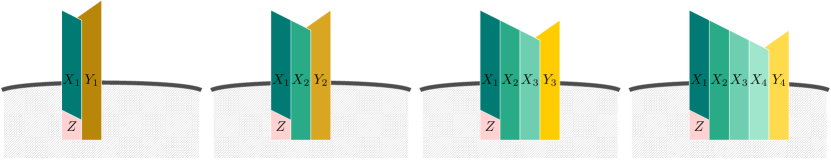
(a) Decoy complexes with kinase.

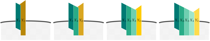
(b) Decoy complexes without kinase.

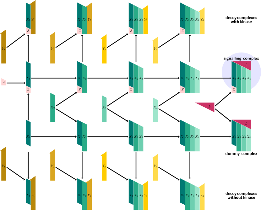
(c) Extended SRLK model: sequential biochemical reaction scheme.

Figure 6: Extended SRLK model with $n=4$ trans-membrane chains: (a) An additional sub-unit chain, $Y_{i}$, can bind to each intermediate signalling complex $Z:X_{1}:\ldots:X_{i}$, to form decoy complexes with kinase. (b) The sub-unit chain $Y_{i}$ can also bind to the intermediate dummy complexes $X_{1}:X_{2}:\ldots:X_{i}$, forming decoy complexes without kinase. (c) Scheme of the sequential formation of the signalling and dummy complexes. At each step their formation can be interrupted by the binding of a sub-unit chain, $Y_{i}$, to the intermediate complex, forming a decoy complex.

We note that while we assume all the $X_{i}$ to be different species, we allow that $Y_{i}=Y_{j}$ or $Y_{i}=\emptyset$, as long as for $i=1,\ldots,n$, $Y_{i}\notin\{X_{1},\ldots,X_{n},Z,L\}$. We assume that the receptor-ligand system is in steady state and the ligand is in excess. We further assume that the concentration of the species $Y_{i}$ (which we write $y_{i}$) are all bounded. We could consider the case when the $Y_{i}$ are in excess, and thus, treat their concentration as a parameter of the model, or assume that the number of $Y_{i}$ molecules is conserved. We refer to these assumptions as the extended experimental hypotheses.

The signalling and dummy functions of classic and extended SRLK receptor-ligand systems are equivalent (see Definition 4.3). The polynomial system describing an extended SRLK model under the extended experimental hypotheses is given by

$$N_{z} =z+K_{0}z(x_{1}(1+K_{y_{1}}y_{1})+\sum_{j=2}^{n}((1+K_{y_{j}}y_{j})\prod_{l=1}^{j-1}K_{l}x_{l}x_{j}))+\sigma(L),$$ (44a)

$$N_{1} =x_{1}(1+K_{y_{1}}^{\prime}y_{1})+\sum_{j=2}^{n}((1+K_{y_{j}}^{\prime}y_{j})\prod_{l=1}^{j-1}K_{l}^{\prime}x_{l}x_{j})+\delta(L)$$ (44b)

$$\quad+K_{0}z(x_{1}(1+K_{y_{1}}y_{1})+\sum_{j=2}^{n}((1+K_{y_{j}}y_{j})\prod_{l=1}^{j-1}K_{l}x_{l}x_{j}))+\sigma(L),$$

$$\vdots$$

$$N_{i} =x_{i}+\sum_{j=i}^{n}((1+K_{y_{j}}^{\prime}y_{j})\prod_{l=1}^{j-1}K_{l}^{\prime}x_{l}x_{j}+K_{0}z(1+K_{y_{j}}y_{j})\prod_{l=1}^{j-1}K_{l}x_{l}x_{j})+\delta(L)+\sigma(L),\quad\text{for }i=2,\ldots,n-1,$$ (44c)

$$\vdots$$

$$N_{n} =x_{n}+K_{0}z(1+K_{y_{n}}y_{n})\prod_{j=1}^{n-1}K_{j}x_{j}x_{n}+(1+K_{y_{n}}^{\prime}y_{n})\prod_{j=1}^{n-1}K_{j}^{\prime}x_{j}x_{n}+\delta(L)+\sigma(L).$$ (44d)

This system of polynomials is completed by the conservation equations of the species $Y_{i}$, for $i=1,\ldots,n$, if we assume they are conserved.

We can extend the notion of no allostery to the extended models.

Definition 4.18.

An extended SRLK model is said to be under the assumption of no allostery if for each $i=1,\ldots,n$, $K_{i}=K_{i}^{\prime}$ and $K_{y_{i}}=K_{y_{i}}^{\prime}$.

With these expanded definitions, we can extend the results previously obtained for the SRLK receptor-ligand systems.

Theorem 4.19.

The theorems and lemmas previously true for the SRLK models are true for the extended SRLK models under the same (extended) hypotheses.

4.4 A few examples of (extended) SRLK models

In spite of some presumably strong modelling assumptions, the (extended) SRLK models can describe a broad range of cytokine-receptor systems. The IL-7R models described in Section 3.1.1 and Section 3.1.2 are, respectively, an SRLK and an extended SRLK model. In this section, we provide examples of other interleukin-signalling systems which are part of the SRLK family.

Example 4.20 (SRLK models: IL-2R and IL-15R).

The interleukin-2 (IL-2) receptor is composed of three trans-membrane sub-unit chains: the common gamma chain, $\gamma$, the IL-2R$\alpha$ chain and the IL-2R$\beta$ chain. Additionally, $\gamma$ binds to the intra-cellular extrinsic kinase JAK3. This IL-2 receptor-ligand system can be considered an SRLK model with $\{Z,X_{1},X_{2},X_{3},L\}=\{\text{JAK3},\gamma,\text{IL-2R}\beta,\text{IL-2R}\alpha,\text{IL-2}\}$. Similarly, the interleukin-15 (IL-15) receptor is composed of three trans-membrane sub-unit chains, $\gamma$, IL-2R$\beta$ and IL-15R$\alpha$, as well as the kinase JAK3. It can be considered an SRLK model with $\{Z,X_{1},X_{2},X_{3},L\}=\{\text{JAK3},\gamma,\text{IL-2R}\beta,\text{IL-15R}\alpha,\text{IL-15}.\}$

A number of interleukin receptors share different molecular components. For instance, cytokine receptors of the common gamma family (comprising the receptors for IL-2,4,7,9,15 and 21 [9]) share the common gamma chain, $\gamma$. In addition the IL-2 and IL-15 receptors share the sub-unit chain, IL-2R$\beta$. The competition for these sub-unit chains can be mathematically described with an extended SRLK model, as follows.

Example 4.21 (Extended SRLK model: IL-2/IL-2R model with formation of IL-7R and IL-15R).

Let us suppose we want to study the formation of IL-2/IL-2R complexes taking into account the competition for the $\gamma$ chain between IL-2R$\beta$ and IL-7R$\alpha$, and the competition for the complex $\gamma:$IL-2R$\beta$ between the sub-units IL-2R$\alpha$ and IL-15R$\alpha$. We can used an extended SRLK model with

$$\{Z,X_{1},X_{2},X_{3},L\}~{}=\{\text{JAK3},\gamma,\text{IL-2R}\beta,\text{IL-2}\alpha,\text{IL-2}\}$$

and

$$\{Y_{1},Y_{2},Y_{3}\}=\{\text{IL-7R}\alpha,\text{IL-15R}\alpha,\emptyset\}.$$

This example is illustrated in Figure 7(a).

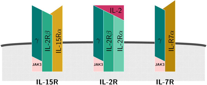
(a) IL-2/IL-2R model with IL-7R and IL-15R competition.

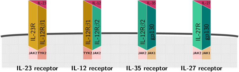
(b) IL-12 receptor family.

Figure 7: (a) Illustration of example 4.21: IL-2R, IL-7R and IL-15R competing for the common gamma chain and IL-2R$\beta$. The IL-2R is composed of three sub-unit chains: the gamma chain, IL-2R$\beta$ and IL-2R$\alpha$. IL-15R is composed of the gamma chain, IL-2R$\beta$ and the specific chain IL-15R$\alpha$. The IL-7R is composed of the gamma chain and IL-7R$\alpha$. All these receptors signal through the Janus kinase JAK3. (b) Illustration of example 4.22: (i) models the competition for IL-12R$\beta$1 between the IL-12 and the IL-23 receptors. We assume that IL-23R and IL-12R$\beta$2 are already bound to their associated extrinsic kinase JAK2; (ii) models the competition for IL-12R$\beta$2 between the IL-12 and IL-35 receptors. We consider the complexes IL-12R$\beta$1:TYK2 and gp130:JAK1 already pre-formed; (iii), models the competition for gp130 between the IL-35 and the IL-27 receptors. We consider the complexes IL-12R$\beta$2:JAK2 and IL-27R:JAK2 already pre-formed.

A further extended SRLK example is that of the IL-12 family of receptors, which share multiple components [55], and each of which is composed of two trans-membrane sub-unit chains. The IL-12 receptor is composed of the sub-unit chains IL-12R$\beta$1 and IL-12R$\beta$2. The IL-23 receptor signals via the IL-23R chain and the IL-12R$\beta$2 chain. The IL-27R (also known as WSX-1) and glycoprotein 130 (gp130) form the IL-27 receptor. Finally, IL-12R$\beta$2 and gp130 form the IL-35 receptor. The sub-unit chains gp130, IL-12R$\beta$1 and IL-12R$\beta$2 bind to a kinase from the JAK family (JAK1, TYK2 and JAK2 respectively). This competition can be described with extended SRLK models as follows.

Example 4.22 (Extended SRLK models: IL-12R family).

We provide three examples of extended SRLK systems which characterise the competition for receptor sub-units between receptors of the IL-12 family (see Figure 7(b)).

1. Suppose we want to study the IL-12-induced signalling process taking into account the competition for IL-12R$\beta$1. We can use an extended SRLK model with

   $$\{Z,X_{1},X_{2},L,Y_{1},Y_{2}\}=\{\text{TYK2},\text{IL-12R}\beta 1,\text{IL-12R}\beta 2^{*},\text{IL-12},\text{IL-23R}^{*},\emptyset\}.$$

2. To study IL-35-induced signalling taking into account the competition for IL-12R$\beta$2, we can use an extended SRLK model with

   $$\{Z,X_{1},X_{2},L,Y_{1},Y_{2}\}=\{\text{JAK2},\text{IL-12R}\beta 2,\text{gp130}^{*},\text{IL-35},\text{IL-12R}\beta 1^{*},\emptyset\}.$$

3. An extended SRLK model with

   $$\{Z,X_{1},X_{2},L,Y_{1},Y_{2}\}=\{\text{JAK1},\text{gp130},\text{IL-27R}^{*},\text{IL-27},\text{IL-12R}\beta 2^{*},\emptyset\}$$

   can describe the IL-27-induced signalling, when there is competition for the sub-unit chain gp130 with the IL-35 receptor.

Above we have made use of the notation $X^{*}$ to denote the pre-formed complex composed of the receptor chain $X$ and its intra-cellular extrinsic kinase (TYK2 for IL-12R$\beta$1, JAK1 for gp130 and JAK2 for all the others).

5 Conclusion

In the first part of this paper we propose a method to compute analytic expressions for two relevant pharmaco-dynamic metrics, the amplitude and the EC₅₀ for receptor-ligand systems, based on two (simple) IL-7 receptor models. Our method starts with the computation of a Gröbner basis for the polynomial system of the receptor-ligand system in steady state. As shown in our IL-7R models from Section 3.1.1 and Section 3.1.2, the derivation of the amplitude is easier when the maximum of the dose-response curve is attained at large ligand concentration (for instance when the dose-response curve is a sigmoid). In that case, the amplitude is the limit of the signalling function when the ligand concentration tends to infinity. When the model is simple enough, as is the case of the first IL-7R model, the polynomial system, simplified by the computation of the Gröbner basis, can be solved iteratively to obtain an analytic expression for the steady state. From these expressions, it is then relatively straightforward to compute the amplitude (i.e., the limit of the signalling function at large values of the ligand concentration) and the EC₅₀. For more complex models, such as our second IL-7R model, getting such steady state expressions can be more challenging. However, perturbation theory can be used to derive the expression for the amplitude. Computing another Gröbner basis can dramatically simplify the calculation of the EC₅₀, and in turn display how it depends on the parameters of the model. Analytic expressions for the amplitude and the EC₅₀ offer mechanistic insight for the receptor-ligand systems under consideration, allow one to quantify the parameter dependency of these two key variables, and can facilitate model validation and parameter exploration. Indeed, for both IL-7R models, we noticed that the affinity constant of the association of the gamma chain to the kinase JAK3, $K_{1}$, was the only constant involved in the expression for the amplitude. As a consequence, and if conducting parameter inference to fit the model to experimental data, $K_{1}$ would be the only parameter that could be inferred by comparison of the theoretical to the experimental amplitude. On the contrary, this constant was absent from both EC₅₀ expressions and thus, its value would be impossible to infer by only comparing the experimental to the theoretical EC₅₀. Our exact analysis also showed that both models have the same amplitude. Finally, the application of our method no longer requires the numerical computation of the dose-response curve, finding its maximum to then obtain the amplitude and fit the curve to derive the EC₅₀. This reduces dramatically the computational cost and numerical errors. However, our method requires models simple enough to be able to compute a lex Gröbner basis, which is known to be computationally intensive [46, 56]. Additionally, computing the amplitude when the maximum response is not the asymptotic behaviour of the dose-response curve can be tricky. For instance the computation of the maximum for bell-shaped dose-response curves (which has been done for simple models in Refs. [35, 36]) may involve the computation of the derivative of the signalling function. This computation can be laborious even with the use of symbolic software. Finally, our method often requires additional mathematical tools or knowledge, such as perturbation theory in Section 3.1.2, which makes it rather a challenge to be used by those who are not mathematically trained. In spite of the (sometimes, complicated) calculations that our method requires, we believe that analytic expressions of the pharmacological metrics characterising simple receptor-ligand systems may provide significant advantages when studying such biological systems.

In the second part of this paper, we introduced a family of receptor-ligand systems, called SLRK, in which the signalling complex, composed of a kinase, a ligand and $n$ trans-membrane sub-unit chains, is built sequentially. These models could also form dummy and decoy complexes, similarly to the IL-7R models which the SRLK family encompasses. By manipulating the polynomials describing the SRLK models, we are able to derive an analytic expression of the amplitude under the no allostery assumption. We also show that the maximum of the dose response curve for both our IL-7R models was indeed the amplitude of the models. Despite relatively strong assumptions, we believe that the SRLK approach can be used to model a broad range of biochemical systems, such as receptor competition in interleukin signalling. The analytic expressions obtained for the amplitude could improve our understanding of biological mechanisms requiring a fine tuning of cytokine signalling such as cancer treatment [57] or cytokine storm control [58, 59]. We showed in Section 4.4 how our SRLK models can account for the competition for the gamma chain between the IL-2 family of receptors and the competition for receptor components between the IL-12 family of receptors. However, many receptors signal through different configurations. IL-35, for instance, can signal through homodimerisation of gp130 or IL-12R$\beta$2 [60]. It has been shown that IL-6, a cytokine implied in cytokine storms [61, 58], signals through an hexameric structure composed of two IL-6R$\alpha$ chains and two gp130 molecules [62]. Furthermore, it seems that the ligand IL-6 first binds to the IL-6R$\alpha$ chain before any association with gp130 [62]. Thus, one could imagine other general receptor models that may involve any of the following: 1) homo-oligomerisation (when two trans-membrane chains $X_{i}$ are identical), 2) other orders of signalling complex formation (non-sequential orders or for instance, if the ligand is not the final sub-unit to be bound), 3) thermodynamic cycles (when there are several ways to form the signalling complex), 4) multiple kinases (including kinases binding to other sub-unit chains, such as JAK1 which binds to IL-7R$\alpha$ [12]), or 5) a more detailed JAK-STAT pathway (most cytokine receptors activate multiple STAT molecules, whose copy numbers tune the immune response elicited [52]).

With this paper we hope to have initiated, or renewed, an interest for the algebraic analysis of receptor-ligand systems. Finally, we believe the results presented in this paper are a first step to account for the variability of receptor expression levels when designing and studying receptor-ligand models (both from an experimental and mathematical perspective) [5, 15, 8, 7].

Appendix A Perturbation theory

A well known difficulty with the lex Göbner basis method, and polynomial equations in general, is that there is usually no analytic solution when the degree of a univariate polynomial is greater than four. This result is known as the Abel-Ruffini theorem [63]. Therefore, in order to make progress, we need to resort to either numerical computations or analytic approximations. Since receptor-ligand systems are often characterised by a sigmoidal dose-response curve, at least to calculate the amplitude, the only quantity of interest is the limit of the signalling function at infinity. In order to calculate this limit (where possible analytically, otherwise numerically) we make use of perturbation theory for polynomial equations.

Greatly inspired by the Dover book written by Simmonds and Mann [54], this section reviews some notions of perturbation theory and justifies the steps of the method used to compute the analytic amplitude expression in Section 3.1.2. We start by defining an asymptotic expansion.

Definition A.1 (Asymptotic expansion).

We say that

$$\sum_{n=0}^{N}\;c_{n}\;f_{n}(\epsilon),$$

is an asymptotic expansion of $f$ in $\epsilon$ if:

• $\{f_{n}\}_{n=0,\ldots,N+1}$ is a gauge sequence, i.e., $f_{n}(\epsilon)=o(f_{n-1}(\epsilon))$ as $\epsilon\to 0$, for $n=0,\ldots,N+1$, and

• $f(\epsilon)-\sum_{n=0}^{N}\;c_{n}\;f_{n}(\epsilon)=\mathcal{O}(\epsilon^{N+1})$ as $\epsilon\to 0.$

The core of perturbation theory is the notion of asymptotic expansion and the following fundamental theorem.

Theorem A.2 (Fundamental theorem of perturbation theory).

If an asymptotic expansion satisfies

$$A_{0}+A_{1}\epsilon+A_{2}\epsilon^{2}+\ldots+A_{n}\epsilon^{N}+\mathcal{O}(\epsilon^{N+1})=0,$$

for any sufficiently small $\epsilon$, and the coefficients $A_{i}$ are independent of $\epsilon$, then we have

$$A_{0}=A_{1}=\ldots A_{N}=0.$$

We are now ready to study the behaviour of the root of a univariate polynomial. Let $n\in\mathbb{N}^{*}$, where $\mathbb{N}^{*}$ is the set of natural numbers without zero. We consider a univariate polynomial, $P_{\epsilon}(x)$, of degree $n$, in the variable $x$, with coefficients which depend on the parameter $\epsilon$. We are interested in the behaviour of the roots of $P_{\epsilon}(x)$ when $\epsilon\to 0$. This polynomial can be re-written in the following form

$$P_{\epsilon}(x)=(1+b_{0}\epsilon+c_{0}\epsilon^{2}+\ldots)+A_{1}\epsilon^{\alpha_{1}}(1+b_{1}\epsilon+c_{1}\epsilon^{2}+\ldots)x+\ldots+A_{n}\epsilon^{\alpha_{n}}(1+b_{n}\epsilon+c_{n}\epsilon^{2}+\ldots)x^{n},$$ (45)

where for each $i$ $\alpha_{i}$ is a rational number, $b_{i}$, $c_{i}$, $\ldots$ are real constants, $(1+b_{i}\epsilon+\ldots)$ is a regular asymptotic expansion of the general from

$$a_{0}+a_{1}\epsilon+\ldots+a_{N}\epsilon^{N}+\mathcal{O}(\epsilon^{N+1}).$$

For such a polynomial, $P_{\epsilon}(x)$, we have the following result.

Theorem A.3.

Each root of a polynomial, such as equation (45) is of the form

$$x(\epsilon)=\epsilon^{p}\omega(\epsilon),\ \ \ \omega(0)\neq 0,$$ (46)

where $\omega$ is a continuous function of $\epsilon$ for $\epsilon$ sufficiently small and $p\in\mathbb{Q}$.

The proof of this theorem (see Ref. [54]) gives a method to study the asymptotic behaviour of the roots of polynomial (45).

Method.

Let $P_{\epsilon}(x)$ be a polynomial that can be written as in equation (45). Let $p$ be a rational and $x$ a root of $P_{\epsilon}$. Let us replace $x$ by $\epsilon^{p}\omega(\epsilon)$ in $P_{\epsilon}$. We can re-write the polynomial as follows

$$P_{\epsilon}(\epsilon^{p}\omega(\epsilon))=Q_{\epsilon}(\omega)+\epsilon(b_{0}+b_{1}A_{1}\epsilon^{\alpha_{1}+p}\omega(\epsilon)+\ldots+b_{n}A_{n}\epsilon^{\alpha_{n}+np}\omega(\epsilon))+\ldots,$$ (47)

where

$$Q_{\epsilon}(\omega)=1+A_{1}\omega(\epsilon)\epsilon^{\alpha_{1}+p}+\ldots A_{n}\omega(\epsilon)\epsilon^{\alpha_{n}+np}.$$

As $\epsilon\to 0$, the dominant term in $P_{\epsilon}$ is the term with the smallest exponent in $Q_{\epsilon}$, i.e., the smallest element of

$$E=\{0,\alpha_{1}+p,\ldots,\alpha_{n}+np\}.$$ (48)

However, the set $E$ must have two identical values. Indeed, if $\alpha_{k}+kp$ is the smallest value of $E$, then we have

$$\epsilon^{-(\alpha_{k}+kp)}P_{\epsilon}(\epsilon^{p}\omega(\epsilon))\underset{\epsilon\to 0}{\sim}A_{k}\omega(0).$$

Since $\omega(0)\neq 0$ and $P_{\epsilon}(\epsilon^{p}\omega(\epsilon))=0$ by hypothesis, we have $A_{k}=0$ which is a contradiction with the fact that $\alpha_{k}+kp\in E$. To select the proper value of $p$, we follow a graphical algorithm which indicates when two or more components of $E$ have equal minimal values:

1. On a plane $(p,q)$, draw the lines $q=\alpha_{j}+jp$, $j=1,\ldots,n$ and the line $q=0$.

2. From the right, for $p$ sufficiently large, the smallest exponent is $0$. As $p$ decreases (one can imagine a fictive vertical line moving from right to left), there will be a first point where at least two lines intersect ($q=0$ and another one). Let us call this point $(p_{1},0)$. One line will have the largest slope, $n_{1}$.

3. Let the fictive vertical line keep moving to the left and follow this line of slope $n_{1}$ until the next intersection $(p_{2},e_{2})$. Find the new intersected line with the largest slope $n_{2}$.

4. Continue until there is no other intersection. The last intersection involves the line with the largest slope of all the lines $n$.

We apply this method on an example and illustrate the algorithm in Section 3.1.2. This algorithm finds all the intersection points of the lines of equation $q=\alpha_{j}+jp$, $j=0,\ldots,n$ and $q=0$ that are on the lower envelop of these lines. In this way, we have generated a set of pairs $\{(p_{j},e_{j})\}_{j=1,\ldots,m}$ corresponding to each intersection we encountered. Each of these intersection points corresponds to an asymptotic behaviour of one branch of the roots of our original polynomial $P_{\epsilon}$. Now let us define for each branch $j$, the scaled polynomial $T^{(j)}_{\epsilon}$, as follows.

$$T^{(j)}_{\epsilon}(\omega)=\epsilon^{-e_{j}}P_{\epsilon}(\epsilon^{p_{j}}\omega).$$ (49)

We can re-write $T^{(j)}_{\epsilon}$ as a sum of two polynomials

$$T_{\epsilon}^{(j)}(\omega)=T_{0}^{(j)}(\omega)+E_{\epsilon}^{(j)}(\omega),$$

where $E_{0}^{(j)}=0$ and $T_{0}^{(j)}$ do not depend on $\epsilon$. The non-zero roots of $T_{\epsilon}^{(j)}$ (approached by the roots of $T_{0}^{(j)}$ as $\epsilon\to 0$) need to be regular but this is not necessarily the case. Indeed, $\alpha_{j}$ or $(p_{j},e_{j})$ may be non-integer rationals or $T_{0}^{(j)}$ may have repeated roots. To obtain regular expansions,, we introduce the new variable $\beta$ such that:

$$\epsilon=\beta^{q_{j}},$$ (50)

where $q_{j}$ is the least common denominator of the set $\{0,\alpha_{1}+p_{j},\ldots\alpha_{n}+np_{j}\}$. Finally, we define

$$R_{\beta}^{(j)}(\omega)=T_{j}(\omega,\beta^{q_{j}})=\beta^{-q_{j}e_{j}}P(\beta^{q_{j}p_{j}}\omega,\beta^{q_{j}})$$ (51)

where $T_{j}(\omega,\epsilon)=T_{\epsilon}^{(j)}(\omega)$ and $P(\omega,\epsilon)=P_{\epsilon}(\omega)$. The polynomial $R_{\beta}^{(j)}$ has the same roots as the polynomial $T_{\epsilon}^{(j)}$ but its non-zero roots have a regular expansion in $\omega$ of the form

$$\omega(\beta)=a_{0}+a_{1}\beta+\ldots+a_{N}\beta^{N}+\mathcal{O}(\beta^{N+1}).$$

By substituting this expansion into $R_{\beta}^{(j)}$ and applying the fundamental theorem of perturbation theory (theorem A.2), we find an expression for $a_{0},a_{1},\ldots$. We then come back to $x$ with the transformation $x=\beta^{q_{j}p_{j}}\omega(\beta)$ for each branch. In practice we explore each branch one by one and can eliminate those which are irrelevant (for instance when we have a negative root, since in our case the roots of the polynomials are concentrations of species, or $\omega(0)=0$).

The above discussion can be summarised algorithmically as follows.

1. Replace the variable $x$ by $\epsilon^{p}\omega(\epsilon)$ in $P_{\epsilon}(x)$, assuming $\omega(0)\neq 0$. One obtains a polynomial of the form $$P_{\epsilon}(\epsilon^{p}\omega(\epsilon))=Q_{\epsilon}(\omega)+\epsilon(\ldots)+\ldots.$$ 2. Write the set of exponents for $Q_{\epsilon}$: $E=\{0,\alpha_{1}+p,\ldots,\alpha_{n}+np\}$. 3. Determine the pairs, $(p_{j},e_{j})$, of proper values and minimal exponents following the graphical algorithm described above. Each pair corresponds to an asymptotic branch to explore. 4. For each branch $j$: 4.1. Define $T^{(j)}_{\epsilon}(\omega)=\epsilon^{-e_{j}}P_{\epsilon}(\epsilon^{p_{j}}\omega)$. 4.2. Introduce $\beta$ such that $\epsilon=\beta^{q}_{j}$, where $q_{j}=\text{lcd}(0,\alpha_{1}+p,\ldots,\alpha_{n}+np)$, and define $R_{\beta}^{(j)}(\omega)=~{}T^{(j)}_{\beta^{q}_{j}}(\omega)$. 4.3. In $R_{\beta}^{(j)}(\omega)=0$, substitute $\omega$ by a regular expansion $\omega(\beta)=a_{0}+a_{1}\beta+\ldots+a_{N}\beta^{N}+\mathcal{O}(\beta^{N+1}).$ 4.4. Apply the fundamental theorem of perturbation theory to obtain an analytic expression for $a_{0},a_{1},\ldots$. Usually at this step, we can discriminate whether this branch is relevant (see example 3.1.2). 4.5. Find the asymptotic expansion of the root of the original polynomial, $P_{\epsilon}$, by $x=\beta^{q_{j}p_{j}}\omega(\beta).$

In this paper we are mainly interested in the first non-zero coefficient of the regular expansion of $\omega$ since it drives the behaviour of the root of $P_{\epsilon}$ in the limit $\epsilon\to 0$.

Appendix B Computation of EC₅₀ for the IL-7R model

We make use of the expression for $\sigma(L)$, the signalling function described in (15), and equation (16), to isolate the square root in equation (20).

$$\sqrt{\Delta_{2}}=K_{2}(K_{3}L_{50}+1)(N_{x}+N_{y})+1-\frac{K_{2}(K_{3}L_{50}+1)^{2}M}{K_{3}L},$$ (52)

with $M=\text{min}(N_{x},N_{y})$. We square the equation to remove the root and simplify the expression to obtain

$$0=4K_{2}^{2}(K_{3}L_{50}+1)^{2}N_{x}N_{y}+K_{2}^{2}(K_{3}L_{50}+1)^{4}\frac{M^{2}}{K_{3}^{2}L_{50}^{2}}-2\frac{K_{2}^{2}(K_{3}L_{50}+1)^{3}M(N_{x}+N_{y})}{K_{3}L_{50}}-2\frac{K_{2}(K_{3}L_{50}+1)^{2}M}{K_{3}L_{50}}.$$ (53)

Since we are looking for a positive value of $L_{50}$, we divide by $K_{2}(K_{3}L_{50}+1)^{2}$ and rewrite the previous expression as follows:

$$0=4K_{2}K_{3}^{2}L_{50}^{2}N_{x}N_{y}+K_{2}(K_{3}L_{50}+1)^{2}M^{2}-2K_{2}(K_{3}L_{50}+1)M(N_{x}+N_{y})K_{3}L_{50}-MK_{3}L_{50}.$$ (54)

It leads to a polynomial of degree $2$ in $L_{50}$,

$$0=M^{2}K_{2}+2K_{3}L_{50}M(-1+K_{2}(M-N_{x}-N_{y}))+K_{3}^{2}K_{2}L_{50}^{2}(M-2N_{x})(M-2N_{y}).$$ (55)

The discriminant of this polynomial is positive:

$$\Delta=[1+K_{2}^{2}(N_{y}-N_{x})^{2}+2K_{2}(N_{x}+N_{y}-M)]4K_{3}^{2}M^{2},$$ (56)

so that there are two potential solutions:

$$L_{50}^{+} =M\frac{1+K_{2}(N_{x}+N_{y}-M)+\sqrt{1+K_{2}^{2}(N_{y}-N_{x})^{2}+2K_{2}(N_{x}+N_{y}-M)}}{K_{2}K_{3}(M-2N_{x})(M-2N_{y})},$$ (57)

$$L_{50}^{-} =M\frac{1+K_{2}(N_{x}+N_{y}-M)-\sqrt{1+K_{2}^{2}(N_{y}-N_{x})^{2}+2K_{2}(N_{x}+N_{y}-M)}}{K_{2}K_{3}(M-2N_{x})(M-2N_{y})}.$$

Two solutions exist since by squaring equation (52) we lose the positive steady state hypothesis. Substituting these expressions back into the steady state equations shows that only $L_{50}^{+}$ leads to a biologically relevant solution. The use of the algebraic method described at the end of Section 3.1.1 is more elegant as it gives directly the correct EC50 expression.

Appendix C Macaulay2 code to compute Gröbner bases

Every Gröbner basis of this paper has been computed making use of Macaulay2 [53]. We provide the code to compute the Gröebner basis of the IL-7R model described in Section 3.1.1.

⬇

R = frac(QQ[Nx,Ny,Nz,L,K1,K2,K3])[x,y,z,MonomialOrder=>Lex]

I = ideal(- Nx + x + K2*x*y + K1*x*z + K2*K_1*x*y*z + K3*K2*L*x*y + K3*K2*K1*L*x*y*z,

- Ny + y + K2*x*y + K2*K_1*x*y*z + K3*K2*L*x*y + K3*K2*K1*L*x*y*z,

- Nz + z + K1*x*z + K2*K_1*x*y*z + K3*K2*K1*L*x*y*z)

g = gens gb I

Appendix D Analytic study of general sequential receptor-ligand systems

D.1 Asymptotic study of the steady states

Lemma 4.7.

Any bounded, continuous solution of ($\dagger$ ‣ 4.5) defined on $\mathbb{R}$ has a finite limit in $+\infty$ (and $-\infty$).

Proof.

Multiply ($\dagger$ ‣ 4.5) by the common denominator of the $R_{i}$ and let $x=\epsilon^{-1}$ to obtain

$$\underbrace{\left[\prod_{i=0}^{m}\tilde{q}_{i}(\epsilon)\right]}_{\tilde{r}_{m}(\epsilon)}\tilde{y}^{m}+\tilde{r}_{m-1}(\epsilon)\tilde{y}^{m-1}+\dots+\tilde{r}_{0}(\epsilon)=0,$$

with $\tilde{y}=\tilde{f}(\epsilon)$. We have now recast the original problem into the form of equation (45). By Theorem A.3 we know, that an expansion for the roots exists and we note that the points of $f(x)$ as $x\to\infty$ correspond to the points of $\tilde{f}(\epsilon)$ as $\epsilon=0$. Note that, since all real $f(x)$ are bounded, so are the real $\tilde{f}(\epsilon)$. Therefore all real $\tilde{f}(0)$ are finite and equal to the limits $\lim_{x\to\infty}f(x)$. A unique limit is chosen by specifying a branch of $f(x)$. The proof for $x\to-\infty$ follows mutatis mutandis. ∎

Lemma 4.8.

The signalling function $\sigma$ and the dummy function $\delta$ of an SRLK model satisfying the experimental hypotheses admit a finite limit when $L\to+\infty$ and this limit is positive.

Proof.

The function $\sigma$ (or $\delta$) are algebraic functions bounded on $\mathbb{R}$ between $0$ and $\text{min}(N_{z},N_{1},\ldots,N_{n})$ (or $\text{min}(N_{1},\ldots,N_{n})$) so they admit a finite limit when $L\to+\infty$. Let us denote this limit by $c_{\sigma}$ (or $c_{\delta}$). We know that $c_{\sigma}$ and $c_{\delta}$ are non-negative because $\sigma$ and $\delta$ are products of non-negative functions.

Consider $c_{\delta}=0$. Then since $\sigma(L)=K_{0}z\prod_{i=1}^{n}\frac{K_{i}}{K_{i}^{\prime}}\delta(L)$, we have $c_{\sigma}=0$ (we note that $z$ being also an algebraic function, $z$ also admits a finite limit when $+\infty$). Since $\delta$ converges to $0$, we need

$$\prod_{i=1}^{n}x_{i}\underset{L\to+\infty}{\sim}\frac{C_{n}}{L^{p}},$$ (58)

with $C_{n}$ a positive constant and $p>1$. We recall and rewrite polynomial (42d):

$$N_{n}=x_{n}+K_{0}z\prod_{i=1}^{n-1}K_{i}\prod_{i=1}^{n}x_{i}+\prod_{i=1}^{n-1}K_{i}^{\prime}\prod_{i=1}^{n}x_{i}+\delta(L)+\sigma(L).$$ (59)

Assuming (58) when $L\to+\infty$ in (59), we obtain:

$$\lim_{L\to+\infty}x_{n}=N_{n},$$

and so we must have

$$\prod_{i=1}^{n-1}x_{i}\underset{L\to+\infty}{\sim}\frac{C_{n-1}}{L^{p}},$$

with $p>1$ and $C_{n-1}$ a positive constant. Passing to the limit in polynomial (42c) for $i=n-1$, we obtain

$$\lim_{L\to+\infty}x_{n-1}=N_{n-1}.$$

We repeat the process for every conservation equation (42c) of the species $X_{i}$ and we obtain

$$\forall i=1,\ldots,n,\ \lim_{L\to+\infty}x_{i}=N_{i},$$

which is a contradiction with equation (58). So $c_{\delta}>0$.

Now, consider $c_{\sigma}=0$. Then since $\sigma(L)=K_{0}z\prod_{i=1}^{n}\frac{K_{i}}{K_{i}^{\prime}}\delta(L)$, $z$ has to tend to $0$. However, when passing to the limit $L\to+\infty$ in equation (42a), we obtain

$$N_{z}=\lim_{L\to+\infty}(z+K_{0}zx_{1}+\ldots+\sigma(L))=0,$$

which is a contradiction.

Conclusion: $c_{\sigma}>0$ and $c_{\delta}>0$. ∎

Lemma 4.9.

In an SRLK model under the experimental hypotheses, the concentration $z$ of the intra-cellular extrinsic kinase $Z$ admits a positive finite limit $c_{z}>0$ when $L\to+\infty$.

Proof.

The concentration of kinase $z$ being an algebraic function bounded on $\mathbb{R}$ between $0$ and $N_{z}$, it admits a finite limit $c_{z}$ when $L\to+\infty$. We know that $c_{z}\geq 0$ because $z$ is a concentration. We now prove that $c_{z}>0$. Since $\delta$ converges to a positive constant when $L\to+\infty$, we must have

$$\prod_{i=1}^{n}x_{i}\underset{L\to+\infty}{\sim}\frac{c_{d}}{L},$$

where $c_{d}$ is a positive constant. Since $\sigma$ also admits a finite limit when $L\to+\infty$, it means that

$$z\prod_{i=1}^{n}x_{i}\underset{L\to+\infty}{\sim}\frac{c_{s}}{L},$$

where $c_{s}$ is a positive constant. So $z$ has to satisfy

$$z\underset{L\to+\infty}{\sim}c_{z},$$

where $c_{z}=\frac{c_{s}}{c_{d}}$ is a positive constant. ∎

Lemma 4.10.

Consider an SRLK model which satisfies the experimental hypotheses. If we assume no allostery, then the steady state value of $z$ is given by

$$z =\frac{-1+K_{1}(N_{z}-N_{1})+\sqrt{\Delta_{z}}}{2K_{1}},$$ (60)

where

$$\Delta_{z} =(1+K_{1}(N_{1}-N_{z}))^{2}+4K_{1}N_{z}.$$

Proof.

We assumed no allostery so $K_{i}=K_{i}^{\prime}$ for all $i=1,\ldots,n$. Equation (42a) gives:

$$N_{z}-z=K_{0}z\left(x_{1}+\sum_{j=2}^{n}\left(\prod_{l=1}^{j-1}K_{l}x_{l}x_{j}\right)+L\prod_{j=1}^{n}K_{j}x_{j}\right)$$

By substituting this equality in equation (42b), we obtain:

$$N_{1}=N_{z}-z+\frac{N_{z}-z}{K_{0}z},$$

so $z$ is a positive root of the polynomial

$$-N_{z}+z(1+K_{1}(N_{1}-N_{z}))+K_{1}z^{2},$$

with $L$-independent coefficients. The two possibilities are:

$$z_{1} =\frac{-1+K_{1}(N_{z}-N_{1})+\sqrt{4K_{1}N_{z}+(1+K_{1}(N_{1}-N_{z}))^{2}}}{2K_{1}},$$

$$z_{2} =\frac{-1+K_{1}(N_{z}-N_{1})-\sqrt{4K_{1}N_{z}+(1+K_{1}(N_{1}-N_{z}))^{2}}}{2K_{1}}.$$

The expression $z_{1}$ is always positive while $z_{2}$ is always negative. Hence $z_{1}$ is the steady state kinase concentration, $z$. ∎

Lemma 4.11.

Let us consider an SRLK model which satisfies the experimental hypotheses. Then no concentration $x_{i}$ behaves proportionally to $L^{q}$, $q>0$ or $\frac{1}{L^{p}}$, $p>1$ when $L\to+\infty$.

Proof.

Lemma 4.9 affirms that $z$ tends to a positive constant when $L\to+\infty$. In order for $\sigma$ or $\delta$ to converge to a positive constant as stated in lemma 4.8, we need

$$\prod_{i=1}^{n}x_{i}\underset{L\to+\infty}{\sim}\frac{c}{L},$$ (61)

where $c$ is a positive constant. Since the concentrations $x_{1},\ldots,x_{n}$ are bounded functions (between 0 and their respective $N_{i}$), it is impossible to have for any $i=1\ldots n$, $x_{i}\underset{L\to+\infty}{\sim}c_{i}L^{q}$ with $c_{i}$ constant and $q>0$. From equation (61) it follows that it is impossible to have any $x_{i}\underset{L\to+\infty}{\sim}\frac{c_{i}}{L^{p}}$ for $p>1$. ∎

Theorem 4.12.

We consider an SRLK model which satisfies the experimental hypotheses. If there exists a unique limiting component $X_{i_{0}}$ then

$$x_{i_{0}}\underset{L\to+\infty}{\sim}\frac{c_{i_{0}}}{L},$$

and for all $i=1,\ldots,n,i\neq i_{0}$,

$$x_{i}\underset{L\to+\infty}{\sim}c_{i},$$

where $c_{i_{0}}$ and $c_{i}$ are positive constants.

Proof.

Since the concentrations $x_{i}$ are algebraic functions (with coefficients in $\mathbb{R}$) bounded on $\mathbb{R}$, they admit a non-negative limit when $L\to+\infty$.

We know that we need

$$\prod_{i=1}^{n}x_{i}\underset{L\to+\infty}{\sim}\frac{c}{L},$$ (62)

with $c$ a positive constant, so that $\sigma$ and $\delta$ converge when $L\to+\infty$. Lemma 4.9 shows that $z$ tends to a positive constant when $L\to+\infty$. Thus, it follows from equation (62) and Lemma 4.11 that at least one of the $x_{i}$ must tend to $0$. We will prove that the only concentration that can tend to $0$ is $x_{i_{0}}$ and so $x_{i_{0}}\underset{L\to+\infty}{\sim}\frac{c_{i_{0}}}{L}$, with $c_{i_{0}}$ a constant.

1) There exists at least one chain $X_{j}$ whose concentration tends to $0$. The conservation equation of $X_{j}$ described in equation (42c) is:

$$N_{j}=x_{j}+\prod_{i=1}^{j}K_{i}^{\prime}x_{i}+K_{0}z\prod_{i=1}^{j}K_{i}x_{i}+\prod_{i=1}^{j+1}K_{i}^{\prime}x_{i}+K_{0}z\prod_{i=1}^{j+1}K_{i}x_{i}+\ldots+\delta(L)+\sigma(L).$$

When $L\to+\infty$, we obtain

$$N_{j}=\lim_{L\to+\infty}\delta(L)+\lim_{L\to+\infty}\sigma(L).$$

We cannot form more dummy or signalling complexes than the number of molecules available. Since $X_{i_{0}}$ is the limiting component, we have

$$\delta(L)+\sigma(L)\leq N_{i_{0}},\ \ \forall L.$$

This yields in the limit $L\to+\infty$, $N_{j}\leq N_{i_{0}}$. By hypothesis this implies means that $j=i_{0}$ and so $X_{j}$ is our limiting component $X_{i_{0}}$.

2) Reciprocally, if $x_{i_{0}}$ tends to a positive constant when $L\to+\infty$, then there exists at least one $x_{j}$, $j\neq i_{0}$ such that $x_{j}\to 0$ when $L\to+\infty$. The limit when $L\to+\infty$ of equation (42c) when $i=j$ gives

$$\lim_{L\to+\infty}[\delta(L)+\sigma(L)]=N_{j}.$$

However, since we also have $\delta+\sigma\leq N_{i_{0}}$, we obtain when taking the limit, $N_{j}\leq N_{i_{0}}$, which is a contradiction with the fact that $X_{i_{0}}$ is the only limiting component.

Conclusion: $X_{i_{0}}$ is limiting if and only if its concentration tends to $0$, and we have

$$x_{i_{0}}\underset{L\to+\infty}{\sim}\frac{c_{i_{0}}}{L},$$

and for $i\neq i_{0}$,

$$x_{i}\underset{L\to+\infty}{\sim}c_{i},$$

where $c_{i_{0}}$ and $c_{i}$ are positive constants. ∎

Corollary 4.13.

If an SRLK model, which satisfies the experimental hypotheses, has multiple limiting components $X_{i_{1}},\ldots,X_{i_{r}}$, $i_{1}<\ldots<i_{r}$ then

$$x_{i_{1}}\underset{L\to+\infty}{\sim}\frac{c_{i_{1}}}{L^{p_{1}}},\ldots,x_{i_{r}}\underset{L\to+\infty}{\sim}\frac{c_{i_{r}}}{L^{p_{r}}},$$

where $c_{i_{1}},\ldots c_{i_{r}}$ are positive constants and $p_{1}=\ldots=p_{r}=\frac{1}{r}$. The non-limiting components $x_{i}$ tend to positive constants $c_{i}$ with $i\notin\{i_{1},\ldots,i_{r}\}$.

Proof.

If $X_{i_{1}}$ and $X_{i_{2}}$ are limiting components, they are the only ones whose concentrations, $x_{i_{1}}$ and $x_{i_{2}}$, tend to $0$ when $L\to+\infty$. From equation (62) we can write

$$x_{i_{1}} \underset{L_{\to}+\infty}{\sim}\frac{c_{i_{1}}}{L^{p_{1}}},$$

$$x_{i_{2}} \underset{L_{\to}+\infty}{\sim}\frac{c_{i_{2}}}{L^{p_{2}}},$$

with $c_{i_{1}}$ and $c_{i_{2}}$ constants and $p_{1},p_{2}>0$, such that $p_{1}+p_{2}=1$.

From system (42), we have:

$$N_{i_{1}} =x_{i_{1}}+\sum_{j=i_{1}}^{n}(\prod_{l=1}^{j-1}K_{l}^{\prime}x_{l}x_{j}+K_{0}z\prod_{l=1}^{j-1}K_{l}x_{l}x_{j})+L\prod_{j=1}^{n}K_{j}^{\prime}x_{j}+K_{0}zL\prod_{j=1}^{n}K_{j}x_{j},$$

$$N_{i_{2}} =x_{i_{2}}+\sum_{j=i_{2}}^{n}(\prod_{l=1}^{j-1}K_{l}^{\prime}x_{l}x_{j}+K_{0}z\prod_{l=1}^{j-1}K_{l}x_{l}x_{j})+L\prod_{j=1}^{n}K_{j}^{\prime}x_{j}+K_{0}zL\prod_{j=1}^{n}K_{j}x_{j}.$$

Since $X_{i_{1}}$ and $X_{i_{2}}$ are limiting components, we have $N_{i_{1}}=N_{i_{2}}$ and, if $i_{1}<i_{2}$, we obtain

$$N_{i_{1}}=N_{i_{2}} \leftrightarrow x_{i_{1}}(1+\sum_{j=i_{1}}^{i_{2}-1}(\prod_{l=1}^{j-1}K_{l}^{\prime}\prod_{l=1,l\neq i_{1}}^{j}x_{l}+K_{0}z\prod_{l=1}^{j-1}K_{l}\prod_{l=1,l\neq i_{1}}^{j}x_{l}))=x_{i_{2}}.$$ (63)

Since all the $x_{i}$, with $i\neq i_{1}$, $i\neq i_{2}$, tend to a positive constant when $L\to+\infty$, we have

$$1+\sum_{j=i_{1}}^{i_{2}-1}(\prod_{l=1}^{j-1}K_{l}^{\prime}\prod_{l=1,l\neq i_{1}}^{j}x_{l}+K_{0}z\prod_{l=1}^{j-1}K_{l}\prod_{l=1,l\neq i_{1}}^{j}x_{l})\underset{L\to+\infty}{\sim}C,$$

where $C$ is a positive constant. Thus, we obtain the behaviour of the left side of equation (63)

$$x_{i_{1}}(1+\sum_{j=i_{1}}^{i_{2}-1}(\prod_{l=1}^{j-1}K_{l}^{\prime}\prod_{l=1,l\neq i_{1}}^{j}x_{l}+K_{0}z\prod_{l=1}^{j-1}K_{l}\prod_{l=1,l\neq i_{1}}^{j}x_{l}))\underset{L_{\to}+\infty}{\sim}\frac{Cc_{i_{1}}}{L^{p_{1}}}.$$

Since the right side is given by

$$x_{i_{2}}\underset{L\to+\infty}{\sim}\frac{c_{i_{2}}}{L^{p_{2}}},$$

it results in $p_{1}=p_{2}=\frac{1}{2}$.

If there are $r$ limiting components $x_{i_{1}},\ldots,x_{i_{r}}$, $i_{1}<\ldots<i_{r}$, then we have

$$x_{i_{1}} \underset{L_{\to}+\infty}{\sim} \frac{c_{i_{1}}}{L^{p_{1}}},$$

$$\vdots \vdots$$

$$x_{i_{r}} \underset{L_{\to}+\infty}{\sim} \frac{c_{i_{r}}}{L^{p_{r}}},$$

with $c_{i_{1}},\ldots,c_{i_{r}}$ positive constants, and $p_{1},\ldots,p_{r}>0$ such that $p_{1}+\ldots+p_{r}=1$. We proceed the same way as for the case of two limiting components and we obtain $p_{1}=\ldots=p_{r}=\frac{1}{r}$. ∎

D.2 Asymptotic study of the signalling and dummy functions

Theorem 4.14.

Consider an SRLK model which satisfies the experimental hypotheses. Write $X_{i_{1}},\ldots,X_{i_{r}}$ as the limiting components and $N_{i_{0}}\equiv N_{i_{1}}=\ldots=N_{i_{r}}$ as their corresponding total number per cell. The limit of the signalling function $\sigma$ when $L$ tends to $+\infty$ is

$$\lim_{L\to+\infty}\sigma(L)=\frac{\prod_{i=1}^{n}K_{i}K_{0}c_{z}}{\prod_{i=1}^{n}K_{i}^{\prime}+\prod_{i=1}^{n}K_{i}K_{0}c_{z}}N_{i_{0}}.$$

The limit of the dummy function $\delta$ when $L$ tends to $+\infty$ is

$$\lim_{L\to+\infty}\delta(L)=\frac{\prod_{i=1}^{n}K_{i}^{\prime}}{\prod_{i=1}^{n}K_{i}^{\prime}+\prod_{i=1}^{n}K_{i}K_{0}c_{z}}N_{i_{0}},$$

where

$$c_{z}=\lim_{L\to+\infty}z.$$

Proof.

By definition of $\sigma$ and $\delta$ we have:

$$\delta(L)+\sigma(L)=L\prod_{i=1}^{n}x_{i}\left(\prod_{i=1}^{n}K_{i}^{\prime}+K_{0}z\prod_{i=1}^{n}K_{i}\right),$$

which implies that

$$\lim_{L\to+\infty}[\delta(L)+\sigma(L)]=\lim_{L\to+\infty}\left(L\prod_{i=1}^{n}x_{i}\left(\prod_{i=1}^{n}K_{i}^{\prime}+K_{0}z\prod_{i=1}^{n}K_{i}\right)\right).$$

Using the limit properties and since everything converges, we obtain:

$$\lim_{L\to+\infty}[\delta(L)+\sigma(L])=\lim_{L\to+\infty}\left(L\prod_{i=1}^{n}x_{i}\right)\left(\prod_{i=1}^{n}K_{i}^{\prime}+K_{0}\lim_{L\to\infty}(z)\prod_{i=1}^{n}K_{i}\right).$$

However, theorem 4.12 states that $x_{i_{0}}$ tends to $0$ when $L\to+\infty$. Thus, equation (42c) when $i=i_{0}$ at $L\to+\infty$ gives

$$N_{i_{0}}=\lim_{L\to+\infty}[\delta(L)+\sigma(L)].$$

Consequently since $z\to c_{z}>0$ from lemma 4.9, we obtain:

$$\lim_{L\to+\infty}(L\prod_{i=1}^{n}x_{i})=\frac{N_{i_{0}}}{\prod_{i=1}^{n}K_{i}^{\prime}+K_{0}c_{z}\prod_{i=1}^{n}K_{i}}.$$

We substitute this limit into the expression of $\sigma$ and $\delta$ and obtain the desired expressions. ∎

Corollary 4.15.

Consider the system of Theorem 4.14 and assume there is no allostery. Denote the limiting components by $X_{i_{1}},\ldots,X_{i_{r}}$ and $N_{i_{0}}\equiv N_{i_{1}}=\ldots=N_{i_{r}}$, their corresponding total number per chain. The limit of the signalling function $\sigma$ at $+\infty$ is

$$\lim_{L\to+\infty}\sigma(L)=\frac{K_{0}z}{1+K_{0}z}N_{i_{0}}.$$

The limit of the dummy function $\delta$ at $+\infty$ is

$$\lim_{L\to+\infty}\delta(L)=\frac{N_{i_{0}}}{1+K_{0}z},$$

and $z$ given by equation (43) in Lemma 4.10.

Proof.

Since there is no allostery, we have $K_{i}=K_{i}^{\prime}$ for all $i$. Lemma 4.10 states that $z$ is independent of $L$, thus $c_{z}=z$. Applying these statements in the expressions of the previous theorem, we obtain the expressions of this corollary. ∎

Lemma 4.16.

Consider an SRLK model under the experimental hypotheses. If there is no allostery, then we have

$$\sup\sigma=\lim_{L\to+\infty}\sigma(L).$$

Proof.

Since $X_{i_{0}}$ is the limiting component, we know from Theorem 4.12 that its concentration tends to $0$ when $L\to+\infty$. We have

$$\delta+\sigma\leq N_{i_{0}}=\lim_{L\to+\infty}(\delta+\sigma).$$ (64)

In the no allostery case, $z$ is independent of $L$ and we have $\sigma=K_{0}z\delta$. Thus, equation (64) gives

$$(1+K_{0}z)\delta\leq(1+K_{0}z)\lim_{L\to+\infty}\delta.$$

Hence, we can conclude

$$\lim_{L\to+\infty}\delta=\sup\delta,$$

and

$$\lim_{L\to+\infty}\sigma=\sup\sigma.$$

∎

D.3 SRLK models with additional receptor sub-units

Theorem 4.19.

The theorems and lemmas previously true for the SRLK models are true for the extended SRLK models under the same (extended) hypotheses.

Proof.

The concentrations $y_{i}$ are bounded ($0\leq y_{i}\leq N_{y_{i}}$) algebraic function on $\mathbb{R}$, and therefore admit a limit when $L\to+\infty$. As the expressions of $\sigma$ and $\delta$ are not modified, the addition of the $Y_{i}$ variables to a SRLK model, assuming the extended experimental hypotheses, does not change the proofs of the previous lemmas and theorems. ∎

Funding.

This project has received funding from the European Union’s Horizon 2020 research and innovation programme under the Marie Skłodowska-Curie grant agreement number 764698 (LS and CMP).

Acknowledgements:

We would like to thank Grégoire Altan-Bonnet for inspiring this work and for encouraging us to explore with analytical methods how the dose-response curve depends on receptor expression levels. We thank Elisenda Feliú and Alicia Dickenstein for carefully reading and providing detailed feedback to an earlier version of this manuscript. We also thank Grant Lythe and Martín López-García for their input in some of the early ideas behind this work and for supervising the doctoral project of one of us (LS). This manuscript has been internally reviewed at Los Alamos National Laboratory, and assigned the reference number LA-UR-22-25806 (CMP).

References

- [1] Eva Bianconi, Allison Piovesan, Federica Facchin, Alina Beraudi, Raffaella Casadei, Flavia Frabetti, Lorenza Vitale, Maria Chiara Pelleri, Simone Tassani, Francesco Piva, et al. An estimation of the number of cells in the human body. Annals of human biology, 40(6):463–471, 2013.
- [2] Kevin A Janes and Douglas A Lauffenburger. Models of signalling networks–what cell biologists can gain from them and give to them. J Cell Sci, 126(9):1913–1921, 2013.
- [3] Simon RJ Maxwell and David J Webb. Receptor functions. Medicine, 36(7):344–349, 2008.
- [4] IJ Uings and SN Farrow. Cell receptors and cell signalling. Molecular Pathology, 53(6):295, 2000.
- [5] Ali M Farhat, Adam C Weiner, Cori Posner, Zoe S Kim, Brian Orcutt-Jahns, Scott M Carlson, and Aaron S Meyer. Modeling cell-specific dynamics and regulation of the common gamma chain cytokines. Cell reports, 35(4):109044, 2021.
- [6] H Steven Wiley, Stanislav Y Shvartsman, and Douglas A Lauffenburger. Computational modeling of the egf-receptor system: a paradigm for systems biology. Trends in cell biology, 13(1):43–50, 2003.
- [7] Aaron M Ring, Jian-Xin Lin, Dan Feng, Suman Mitra, Mathias Rickert, Gregory R Bowman, Vijay S Pande, Peng Li, Ignacio Moraga, Rosanne Spolski, et al. Mechanistic and structural insight into the functional dichotomy between il-2 and il-15. Nature immunology, 13(12):1187–1195, 2012.
- [8] Pauline Gonnord, Bastian R Angermann, Kaitlyn Sadtler, Erin Gombos, Pascal Chappert, Martin Meier-Schellersheim, and Rajat Varma. A hierarchy of affinities between cytokine receptors and the common gamma chain leads to pathway cross-talk. Science Signaling, 11(524):eaal1253, 2018.
- [9] Yrina Rochman, Rosanne Spolski, and Warren J Leonard. New insights into the regulation of t cells by c family cytokines. Nature Reviews Immunology, 9(7):480–490, 2009.
- [10] Warren J Leonard, Jian-Xin Lin, and John J O’Shea. The c family of cytokines: basic biology to therapeutic ramifications. Immunity, 50(4):832–850, 2019.
- [11] Douglas A Lauffenburger and Jennifer Linderman. Receptors: models for binding, trafficking, and signaling. Oxford University Press, 1996.
- [12] Jung-Hyun Park, Adam T Waickman, Joseph Reynolds, Mario Castro, and Carmen Molina-París. Il7 receptor signaling in t cells: A mathematical modeling perspective. Wiley Interdisciplinary Reviews: Systems Biology and Medicine, 11(5):e1447, 2019.
- [13] Carmen Molina-Paris, Joseph Reynolds, Grant Lythe, and Mark Christopher Coles. Mathematical model of naive t cell division and survival il-7 thresholds. Frontiers in immunology, 4:434, 2013.
- [14] Ofer Feinerman, Garrit Jentsch, Karen E Tkach, Jesse W Coward, Matthew M Hathorn, Michael W Sneddon, Thierry Emonet, Kendall A Smith, and Grégoire Altan-Bonnet. Single-cell quantification of il-2 response by effector and regulatory t cells reveals critical plasticity in immune response. Molecular systems biology, 6(1):437, 2010.
- [15] Jesse W Cotari, Guillaume Voisinne, Orly Even Dar, Volkan Karabacak, and Grégoire Altan-Bonnet. Cell-to-cell variability analysis dissects the plasticity of signaling of common chain cytokines in t cells. Science signaling, 6(266):ra17–ra17, 2013.
- [16] DG Lambert. Drugs and receptors. Continuing education in anaesthesia critical care & pain, 4(6):181–184, 2004.
- [17] Omer Dushek, Milos Aleksic, Richard J Wheeler, Hao Zhang, Shaun-Paul Cordoba, Yan-Chun Peng, Ji-Li Chen, Vincenzo Cerundolo, Tao Dong, Daniel Coombs, et al. Antigen potency and maximal efficacy reveal a mechanism of efficient t cell activation. Science signaling, 4(176):ra39–ra39, 2011.
- [18] Miro E Raeber, Yves Zurbuchen, Daniela Impellizzieri, and Onur Boyman. The role of cytokines in t-cell memory in health and disease. Immunological reviews, 283(1):176–193, 2018.
- [19] Alejandro V Villarino, Yuka Kanno, John R Ferdinand, and John J O?Shea. Mechanisms of jak/stat signaling in immunity and disease. The Journal of Immunology, 194(1):21–27, 2015.
- [20] Grégoire Altan-Bonnet and Ratnadeep Mukherjee. Cytokine-mediated communication: a quantitative appraisal of immune complexity. Nature Reviews Immunology, page 1, 2019.
- [21] B Alexander, DJ Browse, SJ Reading, and IS Benjamin. A simple and accurate mathematical method for calculation of the ec50. Journal of pharmacological and toxicological methods, 41(2-3):55–58, 1999.
- [22] Rudolf Gesztelyi, Judit Zsuga, Adam Kemeny-Beke, Balazs Varga, Bela Juhasz, and Arpad Tosaki. The hill equation and the origin of quantitative pharmacology. Archive for history of exact sciences, 66(4):427–438, 2012.
- [23] Sylvain Goutelle, Michel Maurin, Florent Rougier, Xavier Barbaut, Laurent Bourguignon, Michel Ducher, and Pascal Maire. The hill equation: a review of its capabilities in pharmacological modelling. Fundamental & clinical pharmacology, 22(6):633–648, 2008.
- [24] Zheng Chen, Riccardo Bertin, and Guglielmina Froldi. Ec50 estimation of antioxidant activity in dpph assay using several statistical programs. Food chemistry, 138(1):414–420, 2013.
- [25] Jin-Li Li, Xiang-Yang Liu, Jia-Tao Xie, Ya-Li Di, and Fu-Xing Zhu. A comparison of different estimation methods for fungicide ec50 and ec95 values. Journal of Phytopathology, 163(4):239–244, 2015.
- [26] Xiaoqi Jiang and Annette Kopp-Schneider. Summarizing ec50 estimates from multiple dose-response experiments: A comparison of a meta-analysis strategy to a mixed-effects model approach. Biometrical Journal, 56(3):493–512, 2014.
- [27] Rungsiri Suriyatem, Rafael A Auras, Pilairuk Intipunya, and Pornchai Rachtanapun. Predictive mathematical modeling for ec50 calculation of antioxidant activity and antibacterial ability of thai bee products. Journal of Applied Pharmaceutical Science, 7(9):122–133, 2017.
- [28] James Macdougall. Analysis of dose–response studies—e max model. In Dose finding in drug development, pages 127–145. Springer, 2006.
- [29] Neal Thomas. Hypothesis testing and bayesian estimation using a sigmoid e max model applied to sparse dose-response designs. Journal of biopharmaceutical statistics, 16(5):657–677, 2006.
- [30] G Enrico Rovati and Simonetta Nicosia. Lower efficacy: interaction with an inhibitory receptor or partial agonism? Trends in pharmacological sciences, 15(5):140–144, 1994.
- [31] Giovanni Y Di Veroli, Chiara Fornari, Ian Goldlust, Graham Mills, Siang Boon Koh, Jo L Bramhall, Frances M Richards, and Duncan I Jodrell. An automated fitting procedure and software for dose-response curves with multiphasic features. Scientific reports, 5(1):1–11, 2015.
- [32] Raluca Eftimie, Joseph J Gillard, and Doreen A Cantrell. Mathematical models for immunology: current state of the art and future research directions. Bulletin of mathematical biology, 78(10):2091–2134, 2016.
- [33] Jian-Xin Lin and Warren J Leonard. The common cytokine receptor chain family of cytokines. Cold Spring Harbor perspectives in biology, 10(9):a028449, 2018.
- [34] Johan Gabrielsson, Lambertus A Peletier, and Stephan Hjorth. Lost in translation: what’s in an ec50? innovative pk/pd reasoning in the drug development context. European journal of pharmacology, 835:154–161, 2018.
- [35] Eric T Mack, Raquel Perez-Castillejos, Zhigang Suo, and George M Whitesides. Exact analysis of ligand-induced dimerization of monomeric receptors. Analytical chemistry, 80(14):5550–5555, 2008.
- [36] Eugene F Douglass Jr, Chad J Miller, Gerson Sparer, Harold Shapiro, and David A Spiegel. A comprehensive mathematical model for three-body binding equilibria. Journal of the American Chemical Society, 135(16):6092–6099, 2013.
- [37] Martin Feinberg. Chemical reaction network structure and the stability of complex isothermal reactors—i. the deficiency zero and deficiency one theorems. Chemical engineering science, 42(10):2229–2268, 1987.
- [38] Irene Otero-Muras, Pencho Yordanov, and Joerg Stelling. Chemical reaction network theory elucidates sources of multistability in interferon signaling. PLoS computational biology, 13(4):e1005454, 2017.
- [39] Anne Joyce Shiu. Algebraic methods for biochemical reaction network theory. University of California, Berkeley, 2010.
- [40] Ignacio Moraga, Jamie B Spangler, Juan L Mendoza, Milica Gakovic, Tom S Wehrman, Peter Krutzik, and K Christopher Garcia. Synthekines are surrogate cytokine and growth factor agonists that compel signaling through non-natural receptor dimers. Elife, 6:e22882, 2017.
- [41] Joseph Schlessinger. Cell signaling by receptor tyrosine kinases. Cell, 103(2):211–225, 2000.
- [42] Fritz Horn and Roy Jackson. General mass action kinetics. Archive for rational mechanics and analysis, 47(2):81–116, 1972.
- [43] Martin Feinberg. Necessary and sufficient conditions for detailed balancing in mass action systems of arbitrary complexity. Chemical Engineering Science, 44(9):1819–1827, 1989.
- [44] Alicia Dickenstein and Mercedes Pérez Millán. How far is complex balancing from detailed balancing? Bulletin of mathematical biology, 73(4):811–828, 2011.
- [45] Mercedes Pérez Millán and Alicia Dickenstein. Implicit dose-response curves. Journal of Mathematical Biology, 70(7):1669–1684, 2015.
- [46] David Cox, John Little, and Donal O’Shea. Ideals, varieties, and algorithms. undergraduate texts in mathematics, 1997.
- [47] Elizabeth Gross, Heather A Harrington, Zvi Rosen, and Bernd Sturmfels. Algebraic systems biology: a case study for the wnt pathway. Bulletin of mathematical biology, 78(1):21–51, 2016.
- [48] AmirHosein Sadeghimanesh and Elisenda Feliu. Gröbner bases of reaction networks with intermediate species. Advances in Applied Mathematics, 107:74–101, 2019.
- [49] Alicia Dickenstein, Mercedes Perez Millan, Anne Shiu, and Xiaoxian Tang. Multistationarity in structured reaction networks. Bulletin of Mathematical Biology, 81(5):1527–1581, 2019.
- [50] Megan J Palmer, Vinay S Mahajan, Lily C Trajman, Darrell J Irvine, Douglas A Lauffenburger, and Jianzhu Chen. Interleukin-7 receptor signaling network: an integrated systems perspective. Cellular & molecular immunology, 5(2):79–89, 2008.
- [51] Averil Ma, Rima Koka, and Patrick Burkett. Diverse functions of il-2, il-15, and il-7 in lymphoid homeostasis. Annu. Rev. Immunol., 24:657–679, 2006.
- [52] Jian-Xin Lin and Warren J Leonard. Fine-tuning cytokine signals. Annual Review of Immunology, 37:295–324, 2019.
- [53] Daniel R. Grayson and Michael E. Stillman. Macaulay2, a software system for research in algebraic geometry. Available at http://www.math.uiuc.edu/Macaulay2/.
- [54] James G Simmonds and James E Mann. A first look at perturbation theory. Courier Corporation, 2013.
- [55] Dario AA Vignali and Vijay K Kuchroo. Il-12 family cytokines: immunological playmakers. Nature immunology, 13(8):722–728, 2012.
- [56] VA Mityunin and Eugeny V Pankratiev. Parallel algorithms for groebner-basis construction. Journal of Mathematical Sciences, 142(4):2248–2266, 2007.
- [57] Rosanne Spolski, Daniel Gromer, and Warren J Leonard. The c family of cytokines: fine-tuning signals from il-2 and il-21 in the regulation of the immune response. F1000Research, 6, 2017.
- [58] David C Fajgenbaum and Carl H June. Cytokine storm. New England Journal of Medicine, 383(23):2255–2273, 2020.
- [59] Carine Savarin and Cornelia C Bergmann. Fine tuning the cytokine storm by ifn and il-10 following neurotropic coronavirus encephalomyelitis. Frontiers in immunology, 9:3022, 2018.
- [60] Lauren W Collison, Greg M Delgoffe, Clifford S Guy, Kate M Vignali, Vandana Chaturvedi, DeLisa Fairweather, Abhay R Satoskar, K Christopher Garcia, Christopher A Hunter, Charles G Drake, et al. The composition and signaling of the il-35 receptor are unconventional. Nature immunology, 13(3):290–299, 2012.
- [61] Luke YC Chen, Catherine M Biggs, Shahin Jamal, Sophie Stukas, Cheryl L Wellington, and Mypinder S Sekhon. Soluble interleukin-6 receptor in the covid-19 cytokine storm syndrome. Cell Reports Medicine, 2(5):100269, 2021.
- [62] Martin J Boulanger, Dar-chone Chow, Elena E Brevnova, and K Christopher Garcia. Hexameric structure and assembly of the interleukin-6/il-6 -receptor/gp130 complex. Science, 300(5628):2101–2104, 2003.
- [63] Henryk Żołądek. The topological proof of abel-ruffini theorem. Topological Methods in Nonlinear Analysis, 16(2):253–265, 2000.