Benign overfitting and adaptive nonparametric regression

Abstract

In the nonparametric regression setting, we construct an estimator which is a continuous function interpolating the data points with high probability, while attaining minimax optimal rates under mean squared risk on the scale of Hölder classes adaptively to the unknown smoothness.

Contact: julien.chhor@ensae.fr, suzanne.sigalla@ensae.fr, alexandre.tsybakov@ensae.fr

Keywords: Nonparametric regression, Benign overfitting, Local polynomial estimators, Adaptive estimator, Singular kernel, Interpolation, Aggregation.

1 Introduction

Benign overfitting has attracted a great deal of attention in the recent years. It was initially motivated by the fact that deep neural networks have good predictive properties even when perfectly interpolating the training data [Belkin et al., 2019a], [Belkin et al., 2018b], [Zhang et al., 2021], [Belkin, 2021]. Such a behavior stands in strong contrast with the classical point of view that perfectly fitting the data points is not compatible with predicting well. With the aim of understanding this new phenomenon, a series of recent papers studied benign overfitting in linear regression setting, see  [Bartlett et al., 2020], [Tsigler and Bartlett, 2020], [Chinot and Lerasle, 2020], [Muthukumar et al., 2020], [Bartlett and Long, 2021], [Lecué and Shang, 2022] and the references therein. The main conclusion for the linear model is that an unbalanced spectrum of the design matrix and over-parametrization, which in a sense approaches the model to non-parametric setting, are essential for benign overfitting to occur in linear regression. Extensions to kernel ridgeless regression were considered in [Liang and Rakhlin, 2020] when the sample size $n$ and the dimension $d$ were assumed to satisfy $n\asymp d$, and in  [Liang et al., 2020] for a more general case $d\asymp n^{\alpha}$ for $\alpha\in(0,1)$. These papers give data-dependent upper bounds on the risk that can be small assuming favorable spectral properties of the data and the kernel matrix. On the other hand, if $d$ is constant (independent of $n$) then the least-norm interpolating estimator with respect to the Laplace kernel is inconsistent [Rakhlin and Zhai, 2019].

In the line of work cited above, benign overfitting was understood as achieving simultaneously interpolation and prediction consistency, or possibly, consistency with some suboptimal rates. On the other hand, it was shown that, in non-parametric regression setting, interpolating estimators can attain minimax optimal rates [Belkin et al., 2019b]. Namely, it is proved in [Belkin et al., 2019b] that interpolation with minimax optimal rates can be achieved by Nadaraya-Watson estimator with a singular kernel.

The idea of using singular kernels can be traced back to [Shepard, 1968] giving start to popular techniques in image processing referred to as Shepard interpolation. In statistical language, Shepard interpolant is nothing else but the Nadaraya-Watson estimator with kernel $K(u)=1/\|u\|^{2}$, where $\|\cdot\|$ denotes the Euclidean norm and $u\in\mathbf{R}^{2}$. Unaware of Shepard’s work and its subsequent extensive use in image processing, [Devroye et al., 1998] considered the same estimator in general dimension $d$, that is, with the kernel $K(u)=\|u\|^{-d}$ for $u\in\mathbf{R}^{d}$, and proved that the Nadaraya-Watson estimator with such a kernel is consistent in probability but fails to be pointwise almost surely consistent. However, this kernel is not integrable and has a peculiar property that the bandwidth cancels out from the definition of the estimator. Thus, the bias cannot be controlled and the bias-variance trade-off argument based on bandwidth selection does not apply. It remains unclear whether some rates of convergence can be achieved by such an estimator. Therefore, it was suggested in [Belkin et al., 2019b, Belkin et al., 2018c] to localize and modify the kernel as $K(u)=\|u\|^{-a}\mathbf{1}(\|u\|\leq 1)$ where $0<a<d/2$ rather than $a=d$ and $\mathbf{1}(\cdot)$ denotes the indicator function. The estimator with such a weaker type of singularity is also interpolating, and it was shown in [Belkin et al., 2019b, Belkin et al., 2018c] that it achieves the minimax rates of convergence on the $\beta$-Hölder classes with $0<\beta\leq 2$. Also, [Belkin et al., 2018a] proved a similar claim for the $k$ nearest neighbor analog of this estimator with $0<\beta\leq 1$. However, those results were restricted to functions with low smoothness $\beta$ and the suggested estimators were not adaptive to $\beta$.

In this paper, we show that:

• interpolating estimators attaining minimax optimal rates on $\beta$-Hölder classes can be obtained for any smoothness $\beta>0$,

• estimators with such properties can be constructed adaptively to the unknown smoothness $\beta\in(0,\beta_{\max}]$, for any $\beta_{\max}>0$, and to the unknown parameter $L>0$ of the Hölder class of regression functions.

The estimators that we consider to achieve (i) are local polynomial estimators (LPE) with singular kernels. In order to obtain adaptive estimators achieving (ii), we apply aggregation techniques to a family of LPE with singular kernels.

As a by-product, we obtain non-asymptotic bounds for the squared risk of LPE in classical setting with non-singular kernels. To the best of our knowledge, such bounds are missing in the existing literature on LPE that was mainly focused on asymptotic properties such as convergence in probability or pointwise asymptotic normality, cf. [Stone, 1980, Stone, 1982, Tsybakov, 1986, Fan and Gijbels, 1996].

Note that local polynomial method with singular kernels has been used as interpolation tool in numerical analysis, starting from [Lancaster and Salkauskas, 1981]. It was also invoked in the context of non-parametric regression in [Katkovnik, 1985]. However, [Lancaster and Salkauskas, 1981, Katkovnik, 1985] only discussed functional properties, such as the smoothness of interpolants, rather than their statistical behavior.

2 Preliminaries

2.1 Notation

For any vector $x=(x_{1},\dots,x_{d})\in\mathbf{R}^{d}$ and any multi-index $s=(s_{1},\dots,s_{d})\in\mathbf{N}^{d}$, we define

$$\begin{array}[]{lll}\rvert s\rvert=\sum\limits_{i=1}^{d}s_{i},&&s!=s_{1}!\dots s_{d}!\\ &&\\ x^{s}=x_{1}^{s_{1}}\dots x_{d}^{s_{d}}&&D^{s}=\frac{\partial^{s_{1}+\dots+s_{d}}}{\partial x_{1}^{s_{1}}\dots\partial x_{d}^{s_{d}}}.\end{array}$$

We denote by $\|\cdot\|$ the Euclidean norm, and by ${\rm Card}(J)$ the cardinality of set $J$. For any integer $k\in\mathbf{N}^{*}$, we set $[k]=\{1,\dots,k\}$. For any $x\in\mathbf{R}^{d}$, $r>0$, we denote by $\mathscr{B}_{d}(x,r)$ the closed Euclidean ball centered at $x$ with radius $r$. We set for brevity $\mathscr{B}_{d}=\mathscr{B}_{d}(0,1)$. For any $\beta>0$, we denote by $\lfloor\beta\rfloor$ the maximal integer less than $\beta$, and by $\lceil\beta\rceil$ the minimal integer greater than $\beta$. We use symbols $C,C^{\prime}$ to denote positive constants that can vary from line to line.

For any $k>0$, we denote by $I_{k}$ the identity matrix of size $k$. For any square matrix $M$, the writing $M\succ 0$ means that $M$ is positive definite. For any matrix $M$, we denote by $M^{+}$ its Moore-Penrose inverse, and by $\|M\|_{\infty}$ its spectral norm.

2.2 Model

Let $(X,Y)$ be a pair of random variables in $\mathbf{R}^{d}\times\mathbf{R}$ with distribution $P_{XY}$ and assume that we are given $n$ i.i.d. observations $\mathscr{D}:=\left\{(X_{1},Y_{1}),\dots,(X_{n},Y_{n})\right\}$ with distribution $P_{XY}$. We denote by $P_{X}$ the marginal distribution of $X$ and assume that it admits a density $p$ with respect to the Lebesgue measure on the compact set $\text{Supp}(p)$. We assume that for all $x\in\text{Supp}(p)$, the regression function $f(x)=\mathbf{E}(Y\rvert X=x)$ exists and is finite. Set $\xi(X)=Y-\mathbf{E}(Y\rvert X)$. Equivalently, the model can be written as $Y_{i}=f(X_{i})+\xi(X_{i})$, where $\mathbf{E}(\xi(X_{i})|X_{i})=0$. We make the following assumptions.

Assumption $\mathbf{(A1)}$. $\mathbf{E}(|\xi(X)|^{2+\delta}|X=x)\leq C_{\xi}$ for all $x\in\text{Supp}(p)$, where $\delta$ and $C_{\xi}$ are positive constants.

Assumption $\mathbf{(A2)}$. The random vector $X$ is distributed with Lebesgue density $p(\cdot)$ such that $p\in[p_{\min},p_{\max}]$ where $p_{\max}\geq p_{\min}>0$. The support $\text{Supp}(p)$ of $p$ is a convex compact set contained in $\mathscr{B}_{d}$.

For any estimator $f_{n}$ of $f$ based on the sample $\mathscr{D}$, we consider the following $L_{2}$-loss :

$$\|f_{n}-f\|^{2}_{L_{2}}=\mathbf{E}_{X}\left(\left[f_{n}(X)-f(X)\right]^{2}\right)=\int\left[f_{n}(x)-f(x)\right]^{2}p(x)dx,$$

where $\mathbf{E}_{X}$ denotes the expectation with respect to $P_{X}$. We define the expected risk as $\mathbf{E}\left[\|f_{n}-f\|^{2}_{L_{2}}\right],$ where $\mathbf{E}$ denotes the expectation with respect to the distribution of $\mathscr{D}$.

Definition 1 (Interpolating estimator).

An estimator $f_{n}$ of $f$ based on a sample $\mathscr{D}=\{(X_{1},Y_{1}),\dots,(X_{n},Y_{n})\}$ is called interpolating over $\mathscr{D}$ if $f_{n}(X_{i})=Y_{i}$ for $i=1,\dots,n$.

2.3 Hölder classes of functions

For any $k$-linear form $A:(\mathbf{R}^{d})^{k}\longrightarrow\mathbf{R}$, we define its norm as follows

$$\left\|A\right\|_{*}:=\sup\Big{\{}\big{|}A[h_{1},\dots,h_{k}]\big{|}:\|h_{j}\|\leq 1,j\in[k]\Big{\}}.$$ (1)

Given a $k$-times continuously differentiable function $f:\mathbf{R}^{d}\longrightarrow\mathbf{R}$ and $x\in\mathbf{R}^{d}$, we denote by $f^{(k)}(x):(\mathbf{R}^{d})^{k}\longrightarrow\mathbf{R}$ the following $k$-linear form

$$f^{(k)}(x)[h_{1},\dots,h_{k}]=\sum_{|m_{j}|=1,\forall j\in[k]}D^{m_{1}+\dots+m_{k}}f(x)h_{1}^{m_{1}}\dots h_{k}^{m_{k}},\leavevmode\nobreak\ \leavevmode\nobreak\ \forall h_{1},\dots,h_{k}\in\mathbf{R}^{d},$$

where $m_{1},\dots,m_{k}\in\mathbf{N}^{d}$ are multi-indices. Throughout the paper, we will consider the following Hölder class of functions.

Definition 2.

Let $\beta>0$, $L>0$, and let $f:\mathscr{B}_{d}\longrightarrow\mathbf{R}$ be a $\ell=\lfloor\beta\rfloor$ times continuously differentiable function. We denote by $\Sigma(\beta,L)$ the set of all functions $f$ defined on $\mathscr{B}_{d}$ such that

$$\max_{0\leq k\leq\ell}\sup_{x\in\mathscr{B}_{d}}\left\|f^{(k)}(x)\right\|_{*}+\sup_{x,x^{\prime}\in\mathscr{B}_{d}}\frac{\left\|f^{(\ell)}(x)-f^{(\ell)}(x^{\prime})\right\|_{*}}{\|x-x^{\prime}\|^{\beta-\ell}}\leq L.$$

These classes of functions have nice embedding properties that will be needed to prove our result on adaptive estimation. For $\beta^{\prime}\leq\beta\leq 1$, we clearly have $\Sigma(\beta,L)\subseteq\Sigma(\beta^{\prime},L)$. Analogous embedding is valid for $\beta>1$ as stated in the next lemma proved in the Appendix.

Lemma 1.

For any $0<\beta^{\prime}\leq\beta$ and $L>0$ we have $\Sigma(\beta,L)\subseteq\Sigma(\beta^{\prime},2L)$.

The class $\Sigma(\beta,L)$ is closely related to several differently defined Hölder classes used in the literature. One of them is based on Taylor approximation, cf., for example, [Stone, 1980]. For any $x\in\mathbf{R}^{d}$ and any $\ell$ times continuously differentiable real-valued function $f$ on $\mathbf{R}^{d}$, we denote by $Tf_{x}$ its Taylor polynomial of degree $\ell$ at point $x$:

$$Tf_{x}(x^{\prime})=\sum_{0\leq\rvert s\rvert\leq\ell}\frac{(x-x^{\prime})^{s}}{s!}D^{s}f(x^{\prime}).$$

Lemma 2.

Let $\beta>0$, $L>0$ and $f\in\Sigma(\beta,L)$. Then for all $x,y\in\mathscr{B}_{d}$, and $\ell=\lfloor\beta\rfloor$ it holds that

$$\left|f(x)-Tf_{y}(x)\right|\leq\frac{L}{\ell!}\|x\!-\!y\|^{\beta}.$$

Thus, we have $\Sigma(\beta,L)\subseteq\Sigma^{\prime}(\beta,L/\lfloor\beta\rfloor!)$, where $\Sigma^{\prime}(\beta,L^{\prime})$ stands for the class of all functions $f$ satisfying the relation $\left|f(x)-Tf_{y}(x)\right|\leq L^{\prime}\|x\!-\!y\|^{\beta}.$

Next, considering one more definition of Hölder class:

$$\widetilde{\Sigma}(\beta,L)=\left\{f:\mathscr{B}_{d}\rightarrow\mathbf{R}:\sup_{x,x^{\prime}}\frac{\left\|f^{(\ell)}(x)-f^{(\ell)}(x^{\prime})\right\|_{*}}{\|x-x^{\prime}\|^{\beta-\ell}}\leq L\right\}$$

we also immediately have that $\Sigma(\beta,L)\subseteq\widetilde{\Sigma}(\beta,L)$. It follows from [Stone, 1982] that the minimax estimation rate on the class $\widetilde{\Sigma}(\beta,L)$ under the squared loss that we consider below is $n^{-\frac{2\beta}{2\beta+d}}$ up to constants depending only on $\beta$ and $d$. Notice that the functions in $\widetilde{\Sigma}(\beta,L)$ used in the lower bound construction in [Stone, 1982] can be rescaled into functions in $\Sigma(\beta,L)$ by multiplying by a factor depending only on $\beta$ and $d$. Hence, the lower bound construction in [Stone, 1982] remains valid for the class $\Sigma(\beta,L)$. It implies that the minimax rate of estimation on the class $\Sigma(\beta,L)$ is $n^{-\frac{2\beta}{2\beta+d}}$. In conclusion, though $\Sigma(\beta,L)$ is a subclass of suitable Hölder classes $\Sigma^{\prime}$ and $\widetilde{\Sigma}$ it is not substantially smaller, in the sense that estimation over these classes is essentially equally difficult.

3 Local polynomial estimators and interpolation

For $\ell\in\mathbf{N}$ let $C_{\ell,d}={{\ell+d}\choose{d}}$ be the cardinality of the set of multi-indices $\{s=(s_{1},\dots,s_{d})\in\mathbf{N}^{d},0\leq\rvert s\rvert\leq\ell\}$. We assume that the elements $s^{(1)},\dots,s^{(C_{\ell,d})}$ of this set are ordered according to the increasing values of $|s|$, and in an arbitrary way for equal values of $|s|$. In particular, $s^{(1)}=(0,\dots,0)$. For any $u\in\mathbf{R}^{d}$, define the vector $U(u)\in\mathbf{R}^{C_{\ell,d}}$ as follows:

$$U(u):=\left(\frac{u^{s}}{s!}\right)_{\rvert s\rvert\leq\ell},$$

where the components of $U(u)$ are ordered in the same way as $s^{(i)}$’s. In particular, the first component of $U(u)$ is 1 for any $u$.

The definition of local polynomial estimator usually given in the literature is as follows, cf., e.g., [Tsybakov, 2008]. Let $K:\mathbf{R}^{d}\rightarrow\mathbf{R}_{+}$ be a kernel, $h>0$ be a bandwith and $\ell\geq 0$ be an integer. Consider a vector $\hat{\theta}_{n}(x)\in\mathbf{R}^{C_{\ell,d}}$ such that

$$\hat{\theta}_{n}(x)\in\underset{\theta\in\mathbf{R}^{C_{\ell,d}}}{\rm argmin}\ \sum_{i=1}^{n}\left[Y_{i}-\theta^{\top}U\left(\frac{X_{i}-x}{h}\right)\right]^{2}K\left(\frac{X_{i}-x}{h}\right)$$ (2)

Then

$$f_{n}(x)=U^{\top}(0)\hat{\theta}_{n}(x)$$ (3)

is called a local polynomial estimator of order $\ell$ of $f(x)$. Note that $f_{n}(x)$ is the first component of $\hat{\theta}_{n}(x)$.

However, this definition is not convenient for our purposes. First, $\hat{\theta}_{n}(x)$ is not uniquely defined for such $x\in\mathbf{R}^{d}$ that the matrix

$$B_{nx}:=\frac{1}{n{h^{d}}}\sum_{i=1}^{n}U\left(\frac{X_{i}-x}{h}\right)U^{\top}\left(\frac{X_{i}-x}{h}\right)K\left(\frac{X_{i}-x}{h}\right)\in\mathbf{R}^{C_{\ell,d}\times C_{\ell,d}}$$

is degenerate. Furthermore, $\hat{\theta}_{n}(x)$ is not defined for $x=X_{i}$ if the kernel $K$ has a singularity at 0, which will be the main case of interest in what follows. Therefore, we adopt the following slightly different definition.

Definition 3 (Local polynomial estimator).

If the kernel $K$ is bounded then the local polynomial estimator of order $\ell$ (or shortly, LP($\ell$) estimator) of $f(x)$ at point $x$ is defined as

$$f_{n}(x)=\sum_{i=1}^{n}Y_{i}W_{ni}(x),$$ (4)

where, for $i=1,\dots,n$, the weights $W_{ni}(x)$ are given by

$$W_{ni}(x)=\frac{U^{\top}(0)}{n{h^{d}}}B_{nx}^{+}U\left(\frac{X_{i}-x}{h}\right)K\left(\frac{X_{i}-x}{h}\right).$$ (5)

If the kernel $K$ has a singularity at $0$, that is, $\lim_{u\to 0}K(u)=+\infty$, then the LP($\ell$) estimator of $f(x)$ at point $x\notin\{X_{1},\dots,X_{n}\}$ is still defined by (4) while we set, for $j=1,\dots,n$,

$$f_{n}(X_{j})=\limsup\limits_{z\to X_{j}}f_{n}(z).$$ (6)

The purpose of (6) is to provide a valid definition for kernels with singularity at 0. We introduce $\limsup$ in (6) for formal reasons. In the cases of our interest described in the next lemma there exists an exact limit in (6): $\lim_{x\to X_{j}}f_{n}(x)=Y_{j}$ for all $j\in[n]$, which means that the estimator $f_{n}$ is interpolating.

Lemma 3.

[Interpolation property of LPE] Let $f_{n}$ be an LP($\ell$) estimator with kernel $K:\mathbf{R}^{d}\to\mathbf{R}_{+}$ having a singularity at $0$, that is, $\lim_{u\to 0}K(u)=+\infty$, and continuous on $\mathbf{R}^{d}\setminus\{0\}$. In particular, there exist $c_{0}>0$ and $\Delta>0$ such that

$$K(u)\geq c_{0}\mathbf{1}(\|u\|\leq\Delta),\quad\forall u\in\mathbf{R}^{d}.$$ (7)

Assume that $X_{1},\dots,X_{n}$ are distinct points in $\mathbf{R}^{d}$ and there exists a constant $\lambda_{1}>0$ such that

$$\sum_{j=1}^{n}U\left(\frac{X_{j}-x}{h}\right)U^{\top}\left(\frac{X_{j}-x}{h}\right)\mathbf{1}\left(\Big{\|}\frac{X_{j}-x}{h}\Big{\|}\leq\Delta\right)\succ\lambda_{1}I_{C_{\ell,d}}$$ (8)

for all $x$ in some neighborhood of $X_{i}$, where $I_{C_{\ell,d}}$ denotes the identity matrix. Then $f_{n}(X_{i})=Y_{i}$.

For $\ell=0$ (corresponding to the Nadaraya-Watson estimator) condition (8) is trivially satisfied since the expression on the left hand side is a positive scalar for any $x$ in a neighborhood of $X_{i}$. For general $\ell$, this condition is satisfied with high probability if $X_{j}$’s are distributed with a density bounded away from zero on its support. Indeed, we have the following result. For $\Delta>0$ consider the matrix

$$\overline{B}_{nx}:=\frac{1}{n{h^{d}}}\sum_{i=1}^{n}U\left(\frac{X_{i}-x}{h}\right)U^{\top}\left(\frac{X_{i}-x}{h}\right)\mathbf{1}\left(\Big{\|}\frac{X_{i}-x}{h}\Big{\|}\leq\Delta\right)\in\mathbf{R}^{C_{\ell,d}\times C_{\ell,d}}.$$

Lemma 4.

Let $h\leq\alpha$, where $\alpha>0$. Let Assumption $(A2)$ be satisfied. Then, the following holds.

(i) For any $\Delta>0$ there exist constants $\lambda_{0}(\ell)>0$, $c>0$ independent of $n$ and $x$ and depending only on $\ell,\alpha,\Delta,d,p(\cdot)$ such that

$$\mathbf{P}\Big{(}\inf_{x\in{\rm Supp}(p)}\lambda_{\min}(\overline{B}_{nx})\geq\lambda_{0}(\ell)\Big{)}\geq 1-c(h^{-d^{2}-d}e^{-nh^{d}/c}+e^{-n^{3}h^{2d}/c}),$$

where $\lambda_{\min}(\overline{B}_{nx})$ is the minimal eigenvalue of $\overline{B}_{nx}$. Moreover, $\lambda_{0}(\ell)\geq\lambda_{0}(\ell^{\prime})$ if $\ell\leq\ell^{\prime}$.

(ii) If $K$ is a kernel satisfying (7) then there exist constants $\lambda_{0}^{\prime}(\ell)>0$, $c^{\prime}>0$ independent of $n$ and $x$ and depending only on $\ell,\alpha,\Delta,d,p(\cdot)$ such that

$$\mathbf{P}\Big{(}\inf_{x\in{\rm Supp}(p)}\lambda_{\min}(B_{nx})\geq\lambda_{0}^{\prime}(\ell)\Big{)}\geq 1-c^{\prime}(h^{-d^{2}-d}e^{-nh^{d}/c^{\prime}}+e^{-n^{3}h^{2d}/c^{\prime}}).$$

Note that part (ii) of Lemma 4 is an immediate consequence of its part (i) and the fact that $B_{nx}\succ c_{0}\overline{B}_{nx}$ if (7) holds. Also, the next corollary follows immediately from Lemmas 3 and 4.

Corollary 1.

Let $f_{n}$ be an LP($\ell$) with kernel $K:\mathbf{R}^{d}\to\mathbf{R}_{+}$ having a singularity at $0$, that is, $\lim_{u\to 0}K(u)=+\infty$, and continuous on $\mathbf{R}^{d}\setminus\{0\}$. Let $h=\alpha n^{-\frac{1}{2\beta+{d}}}$, where $\alpha,\beta>0$ and let Assumption $(A2)$ be satisfied. Then, there exists a constant $c^{\prime}>0$ such that, with probability at least $1-c^{\prime}e^{-A_{n}/c^{\prime}}$, where $A_{n}=n^{\frac{2\beta}{2\beta+d}}$, the LPE $f_{n}$ is interpolating, that is, $f_{n}(X_{i})=Y_{i}$ for $i=1,\dots,n$, and $f_{n}(\cdot)$ is a continuous function on ${\rm Supp}(p)$. Furthermore, the LP($0$) estimator is interpolating with probability 1.

Note that the kernels $K(u)=\|u\|^{-a}\mathds{1}(\|u\|\leq 1)$ with $a\in(0,{d}/{2})$ considered in [Belkin et al., 2018c, Belkin et al., 2019b] are not continuous on $\mathbf{R}^{d}\setminus\{0\}$ and thus do not satisfy the conditions of Lemma 3 and Corollary 1. On the other hand, these conditions are met for the kernels $K(u)=\|u\|^{-a}\cos^{2}(\pi\|u\|/2)\mathds{1}(\|u\|\leq 1)$ or $K(u)=\|u\|^{-a}(1-\|u\|)_{+}$ with $a>0$.

4 Minimax optimal interpolating estimator

In this section, we show that for any $\beta>0$, one can construct an interpolating local polynomial estimator reaching the minimax rate $n^{-\frac{2\beta}{2\beta+d}}$ on the Hölder class $\Sigma(\beta,L)$.

In what follows, we assume that we know a constant $L_{0}$ such that $|f(x)|\leq L_{0}$ for all $x\in\text{Supp}(p)$. We denote the class of all such functions $f$ by $\mathscr{F}_{0}$. This assumption is not crucial and can be avoided at the expense of slightly more involved dependence of the result on the noise distribution (see Remark 1 below).

Let ${f_{n}}$ be an LP($\ell$) estimator of order $\ell=\lfloor\beta\rfloor$. Set $\mu:=L_{0}\lor\max_{1\leq i\leq n}|Y_{i}|$ and consider the truncated estimator

$$\bar{f}_{n}(x)=\big{[}{f_{n}}(x)\big{]}_{-\mu}^{\mu},$$ (9)

where for all $y\in\mathbf{R}$ and $a\leq b$ the truncation of $y$ between $a$ and $b$ is defined as $[y]_{a}^{b}:=(y\lor a)\land b$.

Theorem 1.

Let Assumptions (A1) and (A2) be satisfied. Let $f\in\Sigma(\beta,L)$ for $\beta>0,L>0$, and $|f(x)|\leq L_{0}$ for all $x\in{\rm Supp}(p)$ and a constant $L_{0}>0$. Consider the estimator $\bar{f}_{n}$ defined in (9), where ${f_{n}}$ is the LP($\ell$) estimator with $\ell=\lfloor\beta\rfloor$, $h=\alpha n^{-\frac{1}{2\beta+{d}}}$, for some $\alpha>0$, and kernel $K$.

(i) If $K$ is a compactly supported kernel satisfying (7) and $\int K^{2}(u)du<\infty$ then

$$\mathbf{E}\left([\bar{f}_{n}(x)-f(x)]^{2}\right) \leq Cn^{-\frac{2\beta}{2\beta+{d}}},\quad\forall x\in{\rm Supp}(p),$$ (10)

$$\mathbf{E}\left(\|\bar{f}_{n}-f\|_{L_{2}}^{2}\right) \leq Cn^{-\frac{2\beta}{2\beta+{d}}},$$ (11)

where $C>0$ is a constant depending only on $\beta,L,L_{0},d,C_{\xi},K,p_{\max},p_{\min}$ and $\alpha$.

(ii) If, in addition, $\lim_{u\to 0}K(u)=+\infty$ and $K$ is continuous on $\mathbf{R}^{d}\setminus\{0\}$, then there exists a constant $c^{\prime}>0$ such that, with probability at least $1-c^{\prime}e^{-A_{n}/c^{\prime}}$, where $A_{n}=n^{\frac{2\beta}{2\beta+d}}$, the estimator $\bar{f}_{n}$ is interpolating, that is, $\bar{f}_{n}(X_{i})=Y_{i}$ for $i=1,\dots,n$, and $\bar{f}_{n}(\cdot)$ is a continuous function on ${\rm Supp}(p)$.

Note that, for the examples of singular kernels given at the end of the previous section, we need $a\in(0,{d}/{2})$ to grant the condition $\int K^{2}(u)du<\infty$ required in Theorem 1. Moreover, Shepard kernel $K(u)=\|u\|^{-d}$ does not satisfy the assumptions of Theorem 1.

Remark 1. The value $\max_{1\leq i\leq n}|Y_{i}|$ is introduced in the threshold $\mu$ only with the aim to preserve the interpolation property. Inspection of the proof shows that Theorem 1(i) remains valid when $\max_{1\leq i\leq n}|Y_{i}|$ is dropped from the definition of $\mu$, so that $\mu=L_{0}$, but in this case data interpolation is not granted. On the other hand, by setting $\mu=2\max_{1\leq i\leq n}|Y_{i}|$ it is possible to obtain both items (i) and (ii) of Theorem 1 for an estimator that does not require the knowledge of $L_{0}$. We do not state this result here since we are able to prove it with the constant $C$ in (10) - (11) depending not only on $C_{\xi}$ but also on a tail property of the distribution of $\xi(X)$ given $X$.

Remark 2. Theorem 1(i) completes the existing literature on LPE in the classical setting when the kernel is non-singular. To the best of our knowledge, non-asymptotic bounds on the mean squared error of LPE were not obtained. The previous work was mainly focused on asymptotic properties such as convergence in probability or pointwise asymptotic normality, cf. [Stone, 1980, Stone, 1982, Tsybakov, 1986, Fan and Gijbels, 1996]. For binary $Y\in\{0,1\}$ specific to classification setting, non-asymptotic deviation bounds for LPE were obtained in [Audibert and Tsybakov, 2007]. However, the techniques of [Audibert and Tsybakov, 2007] cannot be extended beyond the case of bounded $Y$.

Remark 3. Inspection of the proof shows that Theorem 1 extends to kernels $K$ that are not necessarily compactly supported. It suffices to assume that the integrals $\int(1+\|u\|^{\beta})K(u)du$ and $\int(1+\|u\|^{2\beta})K^{2}(u)du$ are finite.

5 Adaptive interpolating estimator

In this section, we will use the following assumption on the noise $\xi(X)$.

Assumption $\mathbf{(A3)}$. Conditionally on $X=x$, the random variable $\xi(X)$ is a zero-mean $\sigma_{\xi}$-subgaussian random variable for all $x\in\text{Supp}(p)$.

We propose an adaptive estimator that does not need the knowledge of $\beta,L,C_{\xi}$, achieves the minimax $L_{2}$-rate of convergence on classes $\Sigma(\beta,L)$ for all $L>0$ and $\beta\in(0,\beta_{\max}]$, where $\beta_{\max}>0$ is an arbitrary given value, and is interpolating with high probability. Our adaptive estimator is based on least squares aggregation. We refer to [Wegkamp, 2003] for the study of such aggregation procedures.

Assume without loss of generality that $n$ is even. We split the sample $\mathscr{D}=\{(X_{1},Y_{1}),\dots,(X_{n},Y_{n})\}$ into two independent subsamples $\mathscr{D}_{1}=\left\{(X_{1},Y_{1}),\dots,(X_{\frac{n}{2}},Y_{\frac{n}{2}})\right\}$ and $\mathscr{D}_{2}=\left\{(X_{\frac{n}{2}+1},Y_{\frac{n}{2}+1}),\dots,(X_{n},Y_{n})\right\}$, and we proceed in two steps.

1. Choose a finite grid $(\beta_{j})_{j\in J}$ on the values of $\beta$. Let $f_{n,j}$ denote a LP($\ell_{j}$) estimator (with $\ell_{j}=\lfloor\beta_{j}\rfloor$) based on the subsample $\mathscr{D}_{1}$ with bandwidth $h=\alpha n^{-\frac{1}{2\beta_{j}+d}}$, $\alpha>0$, and kernel $K$ satisfying the assumptions of Theorem 1. Set $\mu:=L_{0}\lor\max_{1\leq i\leq n/2}|Y_{i}|$ and construct $|J|$ truncated local polynomial estimators:

   $$\bar{f}_{n,j}(x)=\big{[}f_{n,j}(x)\big{]}_{-\mu}^{\mu},\leavevmode\nobreak\ \leavevmode\nobreak\ \leavevmode\nobreak\ \leavevmode\nobreak\ j\in J.$$ (12)

   By Theorem 1, each estimator $\bar{f}_{n,j}$ is interpolating over $\mathscr{D}_{1}$ with high probability, and satisfies

   $$\sup_{f\in\Sigma(\beta_{j},L)\cap\mathscr{F}_{0}}\mathbf{E}_{1}\left[\|\bar{f}_{n,j}-f\|_{L_{2}}^{2}\right]\leq Cn^{-\frac{2\beta_{j}}{2\beta_{j}+d}},$$ (13)

   where $\mathbf{E}_{1}$ denotes the expectation with respect to the distribution of $\mathscr{D}_{1}$.

2. From the collection $(f_{n,j})_{j\in J}$, we select an estimator $\widetilde{f}_{n}$ that minimizes the sum of squares over the second subsample $\mathscr{D}_{2}$, that is, we set $\widetilde{f}_{n}=\bar{f}_{n,\widetilde{j}}$ with

   $$\widetilde{j}\in\underset{j\in J}{\rm argmin}\sum_{k=\frac{n}{2}+1}^{n}\left(Y_{k}-\bar{f}_{n,j}(X_{k})\right)^{2}.$$

As each of the estimators among $(\bar{f}_{n,j})_{j\in J}$ is interpolating over $\mathscr{D}_{1}$, the estimator $\widetilde{f}_{n}$ is also interpolating over $\mathscr{D}_{1}$, but not over $\mathscr{D}_{2}$. We therefore introduce the estimator $\widetilde{g}_{n}$ obtained in the same way as $\widetilde{f}_{n}$ by interchanging $\mathscr{D}_{1}$ and $\mathscr{D}_{2}$. Thus, $\widetilde{g}_{n}$ is interpolating over $\mathscr{D}_{2}$. Next, we define an estimator interpolating over $\mathscr{D}_{1}\cup\mathscr{D}_{2}$ by combining $\widetilde{f}_{n}$ and $\widetilde{g}_{n}$ as follows.

For any $x\in\mathbf{R}^{d}$ and any set $A\subseteq\mathbf{R}^{d}$, denote by $d(x,A)=\inf_{y\in A}\|x-y\|$ the distance between $x$ and $A$. Let $\lambda:\mathbf{R}^{d}\rightarrow[0,1]$ be any continuous function such that $\lambda(x)\to 0$ as $d(x,\mathscr{D}_{2})\to 0$ and $\lambda(x)\to 1$ as $d(x,\mathscr{D}_{1})\to 0$. For example, take $\lambda(x)=\frac{2}{\pi}\arctan\left(\frac{d(x,\mathscr{D}_{2})}{d(x,\mathscr{D}_{1})}\right)$ with $\frac{1}{0}=\infty$ and $\arctan(\infty)=1$ by convention. We define our final estimator as

$$\hat{\sf f}_{n}(x)=\lambda(x){\widetilde{f}_{n}(x)}+(1-\lambda(x)){\widetilde{g}_{n}(x)}.$$ (14)

Theorem 2.

Let $n\geq 3$, $\beta_{\max}>1$. Consider the grid points $\beta_{j}$ defined as follows:

$$\beta_{j}=\left(1+\frac{1}{\log n}\right)^{j},\leavevmode\nobreak\ \leavevmode\nobreak\ j=-M,\dots,M_{\max},$$

where $M=2\left\lfloor\log(n)\log\log(n)\right\rfloor$ and $M_{\max}=M\land\lfloor\log(n)\log(\beta_{\max})\rfloor$. Let Assumptions (A1) and (A3) be satisfied. If kernel $K$ satisfies the assumptions of Theorem 1(i), then for any $\beta\in(0,\beta_{\max}]$ and $L>0$ for the estimator $\hat{\sf f}_{n}$ defined by (14) we have

$$\sup_{f\in\Sigma(\beta,L)\cap\mathscr{F}_{0}}\mathbf{E}\left[\|\hat{\sf f}_{n}-f\|_{L_{2}}^{2}\right]\leq Cn^{-\frac{2\beta}{2\beta+d}},$$ (15)

where $C>0$ is a positive constant depending only on $\beta,L,L_{0},d,\beta_{\max},\sigma_{\xi},K,$ $p_{\max},p_{\min}$ and $\alpha$.

If, in addition, kernel $K$ satisfies the assumptions of Theorem 1(ii), then the estimator $\hat{\sf f}_{n}$ is an interpolating continuous function with probability at least $1-c^{\prime\prime}\exp(-n^{\frac{2}{2+d}}/c^{\prime\prime})$, where $c^{\prime\prime}$ is a positive constant depending only on $L,L_{0},d,\beta_{\max},K,$ $p_{\max},p_{\min}$ and $\alpha$.

6 Numerical experiment

In this section, we report some results of our numerical experiment with singular kernel local polynomial estimators. We ran simulations with various kernels and various regression functions in dimension $d=1$. We present below some examples of obtained results for two regression functions:

$$f(x)=x^{3}-x\quad\text{and}\quad g(x)=x+\cos(3x).$$

We generated $X_{1},\dots,X_{n}$ according to a uniform law on $\left[-2,2\right]$ with $n=80$. We set, for all $i\in\left[n\right]$, $Y_{i}=f(X_{i})+\varepsilon_{i}$ or $Y_{i}=g(X_{i})+\varepsilon_{i}$, where $\varepsilon_{i}$’s are independent normal random variables with mean 0 and variance $0.5$. We considered three singular kernels and the rectangular kernel:

$$K_{1}(u) =\rvert u\rvert^{-a}\mathbf{1}(\rvert u\rvert\leq 1),$$

$$K_{2}(u) =\rvert u\rvert^{-a}\left(1-\rvert u\rvert\right)_{+}^{2},$$

$$K_{3}(u) =\rvert u\rvert^{-a}\cos^{2}(\pi\rvert u\rvert/2)\mathbf{1}(\rvert u\rvert\leq 1),$$

$$K_{\text{rect}}(u) =\mathbf{1}(\rvert u\rvert\leq 1)$$

for various choices of $a\in(0,1/2)$. Below we only present the results for $a=0.2$.

Both $f$ and $g$ belong to Hölder classes with any smoothness $\beta$. We take $\beta=8$ and we compute LP($\ell$) estimators with $\ell=7$ and with bandwidth $h$ chosen, for each kernel, to minimize the mean squared error (MSE) over a dense enough grid. For each singular kernel estimator, we also compute its smoothed version (named Smooth LPE), which is a result of applying the running median with a short window to the initial LPE.

The results are presented below. For comparison, we reproduce in each figure the LPE with rectangular kernel on the right hand graph. Note that $K_{1}$ is not continuous on $\mathbf{R}^{d}\setminus\{0\}$ and therefore does not satisfy the assumptions of Lemma 3 ensuring the interpolation property. Nevertheless, our simulations show that the corresponding LPE does interpolate the data.

The tables present the MSE values. We note that they are bigger for singular kernel estimators than for rectangular kernel ones but not excessively big. It supports the fact that singular kernel LPE achieves the minimax optimal rate, with probably worse constant factor than for its non-singular kernel counterparts. Reasonable MSE values for singular kernel LPE’s are obtained in spite of the fact that visually they are very spiky. The best results are observed for smoothed singular kernel method that cleans out the small spikes. Finally, note that the MSE values are better for function $f$, which itself is a polynomial, than for function $g$.

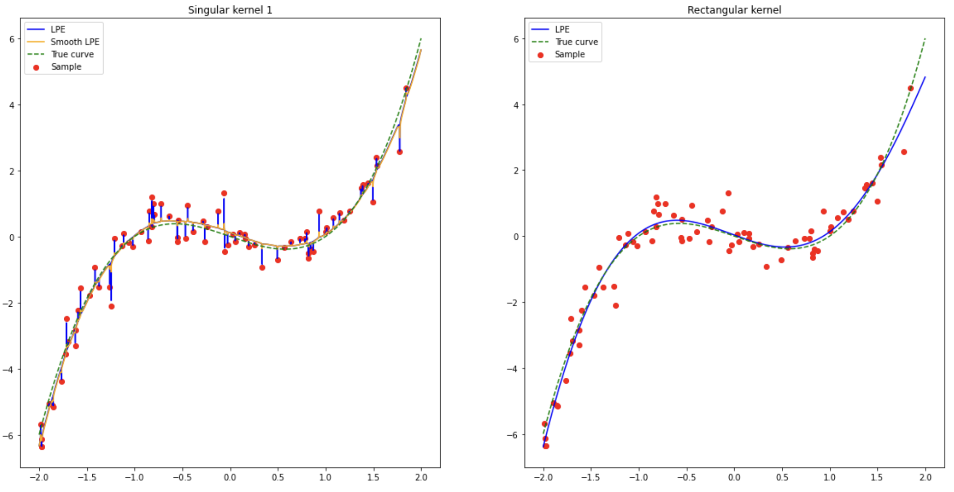
Figure 1: Local polynomial estimator of regression function $f$ with singular kernel $K_{1}$ and rectangular kernel.

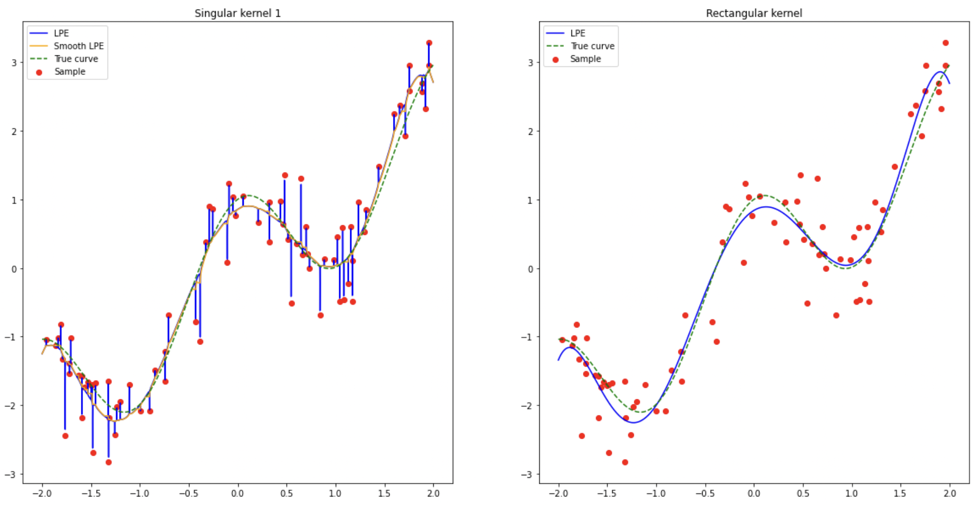
Figure 2: Local polynomial estimator of regression function $g$ with singular kernel $K_{1}$ and rectangular kernel.

	Singular kernel $K_{1}$	Singular Kernel $K_{1}$ + Smooth	Rectangular kernel $K_{\text{rect}}$
Function $f$	0.0373	0.0129	0.0129
Function $g$	0.0424	0.0144	0.0154

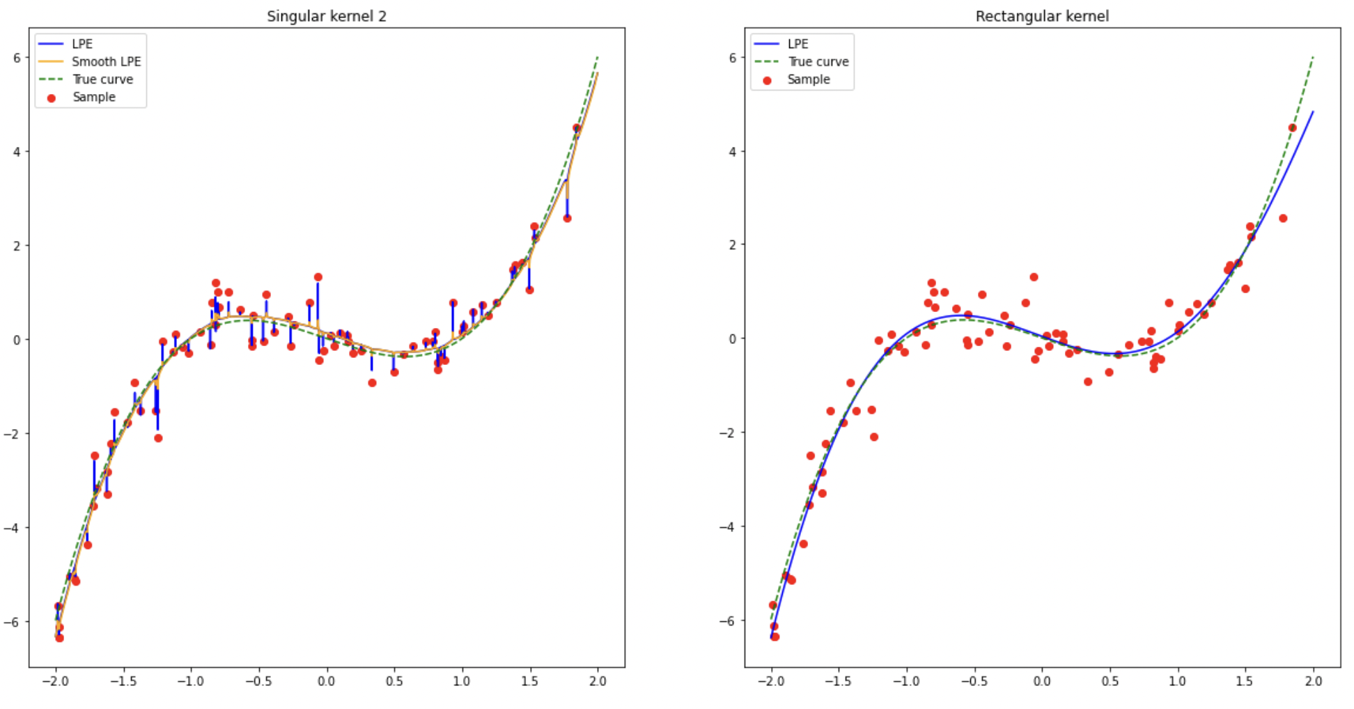
Figure 3: Local polynomial estimator of regression function $f$ with singular kernel $K_{2}$ and rectangular kernel.

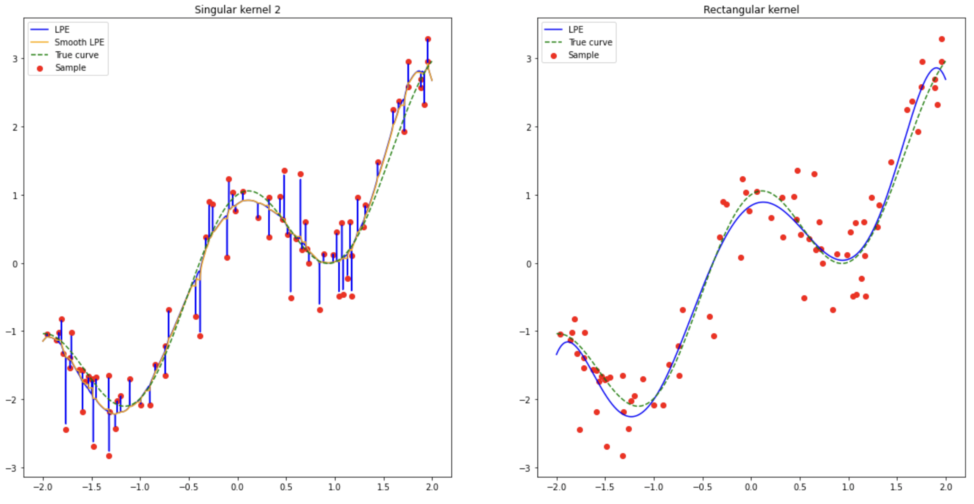
Figure 4: Local polynomial estimator of regression function $g$ with singular kernel $K_{2}$ and rectangular kernel.

	Singular kernel $K_{2}$	Singular kernel $K_{2}$ + Smooth	Rectangular kernel $K_{\text{rect}}$
Function $f$	0.0383	0.0130	0.0129
Function $g$	0.0433	0.0144	0.0154

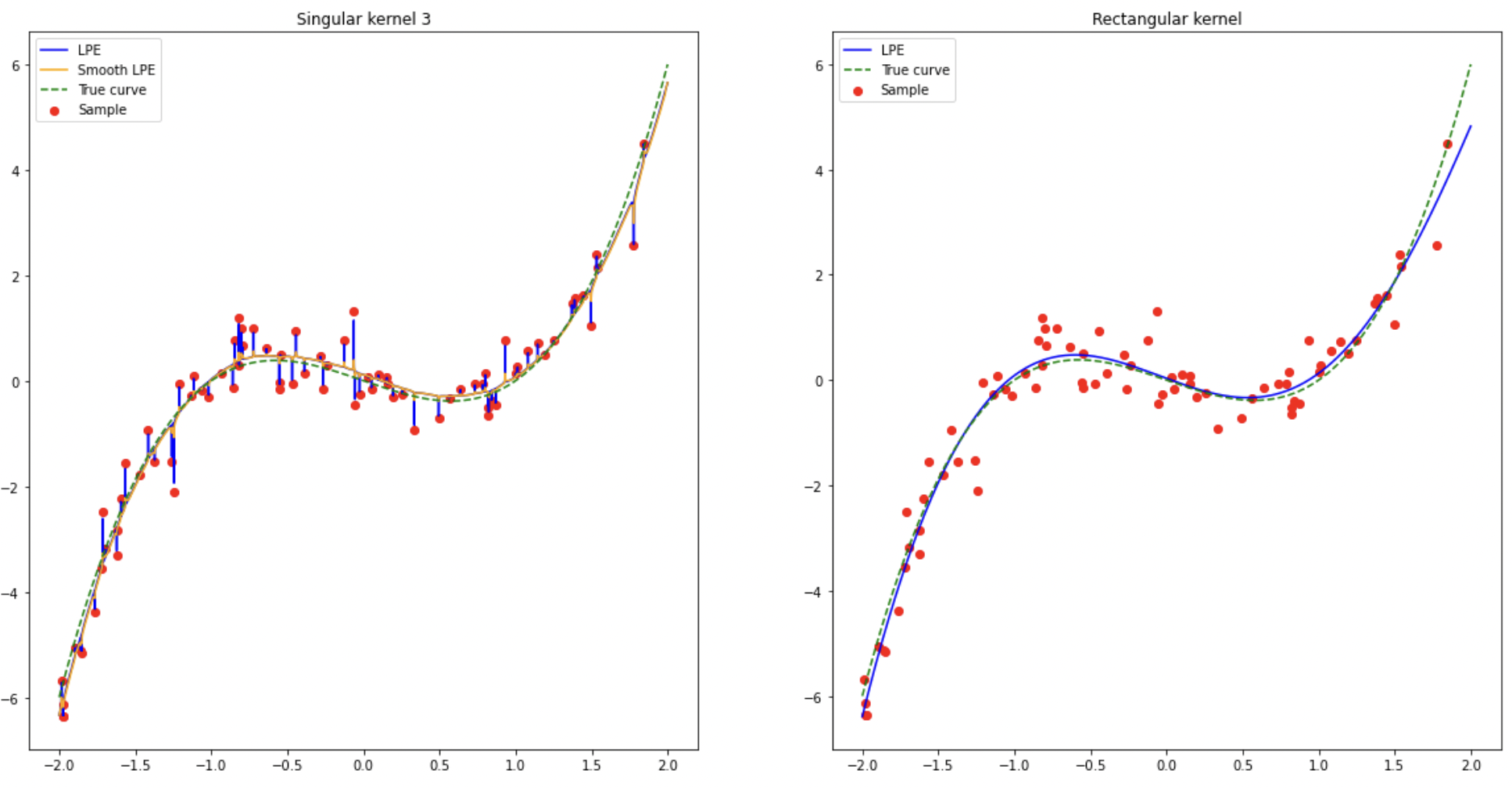
Figure 5: Local polynomial estimator of regression function $f$ with singular kernel $K_{3}$ and rectangular kernel.

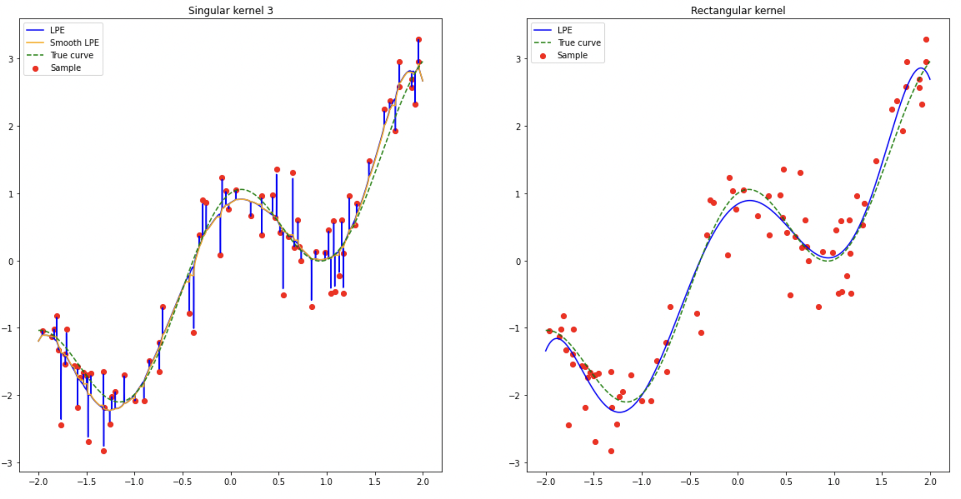
Figure 6: Local polynomial estimator of regression function $g$ with singular kernel $K_{3}$ and rectangular kernel.

	Singular kernel $K_{3}$	Singular kernel $K_{3}$ + Smooth	Rectangular kernel $K_{\text{rect}}$
Function $f$	0.0373	0.0129	0.0129
Function $g$	0.0426	0.0146	0.0154

7 Conclusion

We have shown that local polynomial estimators with singular kernels can achieve minimax optimal rates of convergence (with respect to the mean squared risk) while perfectly interpolating the data, and moreover, can do it adaptively to the the smoothness of the regression function. This seemingly surprising conclusion is indeed not surprising at all because the mean squared risk is used as a criterion. Indeed, by adding "by hand" extremely small spikes to an accurate enough regression estimator we can always get a function interpolating the data and having a reasonably good mean squared risk. Of course, such a construction is very artificial. It makes no sense in practice and it is problematic to achieve adaptation in this way. The miracle of singular kernel LPE is to provide such an effect automatically, including adaptation, as we have outlined above. The resulting interpolating estimators have quite a reasonable behavior in terms of mean squared criterion but not in terms of visual criteria. Note that the interpolating procedures developed in different contexts in the recent literature, in particular, in deep learning are analyzed only in terms of mean squared error and expectedly share the same drawback. The difference from our setting is that, in those models, the resulting estimators are not easy to visualize, so that this sort of "spiky" behavior is not made explicit.

Acknowledgments: This work was supported by the grant of French National Research Agency (ANR) "Investissements d’Avenir" LabEx Ecodec/ANR-11-LABX-0047.

Appendix A Appendix

Proof of Lemma 1.

The result is straightforward if there exists an integer $\ell\geq 0$ such that $\ell<\beta^{\prime}\leq\beta\leq\ell+1$. Indeed, for any integer $\ell\geq 0$,

$$\ell<\beta^{\prime}\leq\beta\leq\ell+1\quad\Longrightarrow\quad\Sigma(\beta,L)\subseteq\Sigma(\beta^{\prime},L).$$ (16)

Thus, it remains to consider the case $\ell<\beta^{\prime}\leq\ell+1<\beta$ for an integer $\ell$. Handling this case will be based on the following embedding:

$$\Sigma(\beta,L)\subseteq\Sigma(\ell^{\prime},2L),\quad\forall\ell^{\prime}\in\mathbf{N}\text{ such that }\ell^{\prime}<\beta.$$ (17)

We now prove (17). Indeed, let $f\in\Sigma(\beta,L)$ and let $\ell^{\prime}$ be an integer less than $\beta$. Then, in particular, $\max\limits_{0\leq s\leq\ell^{\prime}}\sup\limits_{x\in\mathscr{B}_{d}}\left\|f^{(s)}(x)\right\|_{*}\leq L$. Consider $x,y\in\mathscr{B}_{d}$ and $h=y-x$. Denote by $h_{i}$ the $i$th component of $h$ and by $e_{i}$ the $i$th canonical basis vector in $\mathbf{R}^{d}$. Set $k=\ell^{\prime}-1$. Then for any multi-indices $m_{1},\dots,m_{k}\in\mathbf{N}^{d}$ we have

$$D^{m_{1}+\cdots+m_{k}}f(y)-D^{m_{1}+\cdots+m_{k}}f(x) =\int_{0}^{1}\left\langle\nabla D^{m_{1}+\cdots+m_{k}}f(x+th),h\right\rangle dt$$

$$=\int_{0}^{1}\sum_{i=1}^{d}D^{m_{1}+\cdots+m_{k}+e_{i}}f(x+th)h_{i}dt$$

$$=\sum_{i=1}^{d}\int_{0}^{1}D^{m_{1}+\cdots+m_{k}+e_{i}}f(x+th)dt\,h^{e_{i}}.$$

Writing for brevity $G_{m_{1},\dots,m_{k},e_{i}}(x,h)=\int_{0}^{1}D^{m_{1}+\cdots+m_{k}+e_{i}}f(x+th)dt$ we obtain

$$\left\|f^{(k)}(y)-f^{(k)}(x)\right\|_{*}=\sup_{\begin{subarray}{c}\|u_{j}\|\leq 1,\\ j\in[k]\end{subarray}}\Big{|}\sum_{|m_{j}|=1,\forall j\in[k]}\sum_{i=1}^{d}G_{m_{1},\dots,m_{k},e_{i}}(x,h)\,h^{e_{i}}u_{1}^{m_{1}}\dots u_{k}^{m_{k}}\Big{|}$$

$$\qquad=\|h\|\sup_{\begin{subarray}{c}\|u_{j}\|\leq 1,\\ j\in[k]\end{subarray}}\Big{|}\sum_{|m_{j}|=1,\forall j\in[k]}\sum_{i=1}^{d}G_{m_{1},\dots,m_{k},e_{i}}(x,h)\,\left(\frac{h}{\|h\|}\right)^{e_{i}}u_{1}^{m_{1}}\dots u_{k}^{m_{k}}\Big{|}$$

$$\qquad\leq\|h\|\sup_{\begin{subarray}{c}\|u_{j}\|\leq 1,\\ j\in[k+1]\end{subarray}}\Big{|}\sum_{|m_{j}|=1,\forall j\in[k+1]}\int_{0}^{1}D^{m_{1}+\cdots+m_{k+1}}f(x+th)dt\,u_{1}^{m_{1}}\dots u_{k+1}^{m_{k+1}}\Big{|}$$

$$\qquad\leq\|h\|\int_{0}^{1}\sup_{\begin{subarray}{c}\|u_{j}\|\leq 1,\\ j\in[k+1]\end{subarray}}\big{|}f^{(k+1)}(x+th)[u_{1},\dots,u_{k+1}]\big{|}dt$$

$$\qquad\leq\|h\|\sup_{z\in\mathscr{B}_{d}}\|f^{(k+1)}(z)\|_{*}\leq L\|x-y\|,$$

which, together with bound $\max\limits_{0\leq s\leq\ell^{\prime}-1}\sup\limits_{x\in\mathscr{B}_{d}}\left\|f^{(s)}(x)\right\|_{*}\leq L$ implies that $f\in\Sigma(\ell^{\prime},2L)$. Thus, we have proved (17).

It follows from (17) that if $\ell<\beta^{\prime}\leq\ell+1<\beta$ for an integer $\ell$ then $\Sigma(\beta,L)\subseteq\Sigma(\ell+1,2L)$, while taking $\beta=\ell+1$ in (16) implies that $\Sigma(\ell+1,2L)\subseteq\Sigma(\beta^{\prime},2L)$. This proves the lemma when $\ell<\beta^{\prime}\leq\ell+1<\beta$ for an integer $\ell$. ∎

Proof of Lemma 2.

The result is clear for $\beta\leq 1$. Assume that $\beta>1$ and fix some $x,y\in\mathscr{B}_{d}$. By Taylor expansion, there exists $c\in(0,1)$ such that

$$f(x)=\sum_{0\leq|k|\leq\ell-1}\frac{1}{k!}D^{k}\!f(y)(x\!-\!y)^{k}+\sum_{|k|=\ell}\frac{1}{k!}D^{k}\!f(y\!+\!c(x\!-\!y))(x\!-\!y)^{k},$$

and

$$\left|f(x)-\sum_{|k|\leq\ell}\frac{1}{k!}D^{k}\!f(y)(x\!-\!y)^{k}\right| =\left|\sum_{|k|=\ell}\frac{1}{k!}\big{[}D^{k}\!f\big{(}y\!+\!c(x\!-\!y)\big{)}-D^{k}\!f(y)\big{]}(x\!-\!y)^{k}\right|.$$

By a standard combinatorial argument, it is not hard to check that, for any $h,z\in\mathbf{R}^{d}$,

$$f^{(k)}(z)[h]^{k}: =\sum_{|m_{1}|=\ldots=|m_{\ell}|=1}D^{m_{1}+\ldots+m_{\ell}}f(z)h^{m_{1}+\ldots+m_{\ell}}=\sum_{|k|=\ell}\frac{\ell!}{k!}D^{k}f(z)h^{k}\enspace.$$

It follows that

$$\left|\sum_{|k|=\ell}\frac{1}{k!}\big{[}D^{k}\!f\big{(}y\!+\!c(x\!-\!y)\big{)}-D^{k}\!f(y)\big{]}(x\!-\!y)^{k}\right|$$ (18)

$$\qquad=\frac{1}{\ell!}\left|f^{(\ell)}\big{(}y\!+\!c(x\!-\!y)\big{)}[x\!-\!y]^{\ell}-f^{(\ell)}(y)[x\!-\!y]^{\ell}\right|$$

$$\qquad\leq\frac{1}{\ell!}\left\|f^{(\ell)}\big{(}y\!+\!c(x\!-\!y)\big{)}-f^{(\ell)}(y)\right\|_{*}\|x\!-\!y\|^{\ell}$$

$$\qquad\leq\frac{L}{\ell!}\|x\!-\!y\|^{\ell}\|c(x\!-\!y)\|^{\beta-l}\leq\frac{L}{\ell!}\|x\!-\!y\|^{\beta}.$$

∎

Proof of Lemma 3.

In this proof, we fix $i\in\left[n\right]$, and our aim is to prove that $\lim_{x\to X_{i}}f_{n}(x)=Y_{i}$. Let $\mathscr{V}$ be the neighborhood of $X_{i}$ where (8) holds. Since $X_{1},\dots,X_{n}$ are distinct, we assume w.l.o.g. that $\mathscr{V}$ does not contain $(X_{j})_{j\neq i}$. Due to conditions (7) and (8), we have that $B_{nx}\succ 0$ for all $x$ in $\mathscr{V}_{-}:=\mathscr{V}\setminus\{X_{i}\}$. Thus, for all $x\in\mathscr{V}_{-}$ the vector $\hat{\theta}_{n}(x)$ is the unique solution of (2), and $f_{n}(x)$ is given by (3):

$$\hat{\theta}_{n}(x)=\underset{\theta\in\mathbf{R}^{C_{\ell,d}}}{\rm argmin}\ \sum_{i=1}^{n}\left[Y_{i}-\theta^{\top}U\left(\frac{X_{i}-x}{h}\right)\right]^{2}K\left(\frac{X_{i}-x}{h}\right),$$

$$f_{n}(x)=U^{\top}(0)\hat{\theta}_{n}(x).$$

Define $g_{i}(x)=\left(Y_{i}-\hat{\theta}_{n}(x)^{\top}U\left(\frac{X_{i}-x}{h}\right)\right)^{2}$. First, we prove by contradiction that $\lim\limits_{x\rightarrow X_{i}}g_{i}(x)=0$ for any $i\in\left[n\right]$. Indeed, suppose that $\lim_{x\rightarrow X_{i}}g_{i}(x)\neq 0$. Then, there is a sequence $(x_{k})_{k}$ in $\mathbf{R}^{d}$ converging to $X_{i}$ as $k\to\infty$ such that $\lim_{k\to\infty}g_{i}(x_{k})=+\infty$ or $\lim_{k\to\infty}g_{i}(x_{k})={\rm const}>0$. In both cases,

$$\lim_{k\to\infty}\sum_{j=1}^{n}g_{j}(x_{k})K\left(\frac{X_{j}-x_{k}}{h}\right)=+\infty$$ (19)

since the kernel $K$ has a singularity at 0. On the other hand, the definition of $\hat{\theta}_{n}(x_{k})$ implies that, for any $k$ and any $\theta_{*}\in\mathbf{R}^{C_{\ell,d}}$,

$$\sum_{j=1}^{n}g_{j}(x_{k})K\left(\frac{X_{j}-x_{k}}{h}\right)\leq\sum_{j=1}^{n}\left(Y_{j}-\theta_{*}^{\top}U\left(\frac{X_{j}-x_{k}}{h}\right)\right)^{2}K\left(\frac{X_{j}-x_{k}}{h}\right).$$

In particular, for $\theta_{*}^{\top}=\left(Y_{i}\quad 0\dots 0\right)$ we have

$$\sum_{j=1}^{n}\left(Y_{j}-\theta_{*}^{\top}U\left(\frac{X_{j}-x_{k}}{h}\right)\right)^{2}K\left(\frac{X_{j}-x_{k}}{h}\right)= \sum_{j=1}^{n}(Y_{j}-Y_{i})^{2}K\left(\frac{X_{j}-x_{k}}{h}\right)$$

$$= \sum_{j\neq i}(Y_{j}-Y_{i})^{2}K\left(\frac{X_{j}-x_{k}}{h}\right)$$

$$\underset{k\rightarrow+\infty}{\rightarrow} \sum_{j\neq i}(Y_{j}-Y_{i})^{2}K\left(\frac{X_{j}-X_{i}}{h}\right)<+\infty,$$

which is in contradiction with (19). Therefore, for any $i\in\left[n\right]$ we have $\lim\limits_{x\rightarrow X_{i}}g_{i}(x)=0$.

A similar argument yields that $\lim\sup\limits_{x\rightarrow X_{i}}g_{j}(x)<+\infty$ for any $j\neq i$. Indeed, if for some $j\neq i$ this relation does not hold then there is a sequence $(x_{k})_{k}$ in $\mathbf{R}^{d}$ converging to $X_{i}$ as $k\to\infty$ such that $\lim_{k\to\infty}g_{j}(x_{k})=+\infty$. It implies (19), which is not possible as shown above.

Next, we prove that $\|\hat{\theta}_{n}(x)\|$ is bounded for all $x$ in a neighborhood of $X_{i}$. Since $\lim\limits_{x\rightarrow X_{i}}g_{i}(x)=0$, and for any $j\neq i$ we have $\lim\sup\limits_{x\rightarrow X_{i}}g_{j}(x)<+\infty$ the values $g_{j}(x)$ are bounded for all $j\in\left[n\right]$ and all $x$ in a neighborhood of $X_{i}$. We will further denote this neighborhood by $\mathscr{V}^{\prime}$. It follows that $\varphi_{j}(x)=\hat{\theta}_{n}(x)^{\top}U\left(\frac{X_{j}-x}{h}\right)$, $j=1,\dots,n,$ are bounded for $x\in\mathscr{V}^{\prime}$ and thus the sum $\sum_{j=1}^{n}\varphi_{j}^{2}(x)$ is bounded as well. On the other hand, by assumption (8), for all $x\in\mathscr{V}_{-}$,

$$\sum_{j=1}^{n}\varphi_{j}^{2}(x) \geq\sum_{j=1}^{n}\hat{\theta}_{n}(x)^{\top}U\left(\frac{X_{j}-x}{h}\right)U^{\top}\left(\frac{X_{j}-x}{h}\right)\mathbf{1}\left(\left\|\frac{X_{j}-x}{h}\right\|\leq\Delta\right)\hat{\theta}_{n}(x)$$

$$\geq\lambda_{1}\|\hat{\theta}_{n}(x)\|^{2},$$

where $\lambda_{1}>0$. It follows that $\|\hat{\theta}_{n}(x)\|$ is bounded for all $x\in\mathscr{V}^{\prime}\cap\mathscr{V}_{-}$.

Let $\hat{\theta}_{n,(1)}(x)=f_{n}(x)$ denote the first component of $\hat{\theta}_{n}(x)$ and $\hat{\theta}_{n,(2)}(x)$ the vector of its remaining $C_{\ell,d}-1$ components, so that $\hat{\theta}_{n}(x)^{\top}=\left(\hat{\theta}_{n,(1)}(x),\hat{\theta}_{n,(2)}(x)^{\top}\right)$. Recall that the first component of $U(u)$ is equal to 1 for all $u\in\mathbf{R}^{d}$. Denote by $U_{(2)}(u)$ the vector of its remaining $C_{\ell,d}-1$ components, so that $U(u)^{\top}=\left(1,U_{(2)}(u)^{\top}\right)$. With this notation, the relation $\lim\limits_{x\rightarrow X_{i}}g_{i}(x)=0$ proved above can be written as:

$$g_{i}(x) =\left(Y_{i}-\hat{\theta}_{n,(1)}(x)-\hat{\theta}_{n,(2)}(x)^{\top}U_{(2)}\left(\frac{X_{i}-x}{h}\right)\right)^{2}\underset{x\rightarrow X_{i}}{\rightarrow}0.$$

Since $\|\hat{\theta}_{n}(x)\|$ is bounded for $x\in\mathscr{V}^{\prime}\cap\mathscr{V}_{-}$ we get that $|\hat{\theta}_{n,(1)}(x)|$ and $\|\hat{\theta}_{n,(2)}(x)\|$ are also bounded for $x\in\mathscr{V}^{\prime}\cap\mathscr{V}_{-}$. The definition of $U(u)$ implies the convergence $\lim\limits_{x\rightarrow X_{i}}\|U_{(2)}\left(\frac{X_{i}-x}{h}\right)\|=0$. It follows that

$$\hat{\theta}_{n,(2)}(x)^{\top}U_{(2)}\left(\frac{X_{i}-x}{h}\right)\underset{x\rightarrow X_{i}}{\rightarrow}0$$

and therefore

$$\hat{\theta}_{n,(1)}(x)\underset{x\rightarrow X_{i}}{\rightarrow}Y_{i},$$

which concludes the proof since $\hat{\theta}_{n,(1)}(x)=f_{n}(x)$. ∎

Proof of Lemma 4.

We prove only part (i) of the lemma since part (ii) is its immediate consequence. We have

$$\overline{B}_{nx}=\frac{1}{n{h^{d}}}\sum_{i=1}^{n}U\left(\frac{X_{i}-x}{h}\right)U^{\top}\left(\frac{X_{i}-x}{h}\right)\mathbf{1}\left(\frac{\|X_{i}-x\|}{\Delta}\leq h\right)$$

and, for any $\lambda_{0}>0$,

$$\mathbf{P}\left(\inf_{x\in{\rm Supp}(p)}\lambda_{\min}(\overline{B}_{nx})<\lambda_{0}\right)=\mathbf{P}\left(\inf_{x\in{\rm Supp}(p)}\inf_{\|v\|=1}v^{\top}\overline{B}_{nx}v<\lambda_{0}\right)$$

$$\leq\mathbf{P}\left(\inf_{x\in{\rm Supp}(p)}\inf_{\|v\|=1}\!v^{\top}\overline{B}(x)v-\sup_{x\in{\rm Supp}(p)}\|\overline{B}_{nx}\!-\!\overline{B}(x)\|_{\infty}<\lambda_{0}\right)$$ (20)

where $\overline{B}(x):=\mathbf{E}(\overline{B}_{nx})$. Set $S(x,h,\Delta)=\left\{u\in\mathscr{B}_{d}(0,\Delta):x+uh\in{\rm Supp}(p)\right\}$. Then we have

$$v^{\top}\overline{B}(x)v ={\frac{1}{h^{d}}}\int\left[v^{\top}U\left(\frac{z-x}{h}\right)\right]^{2}\mathbf{1}\left(\left\|\frac{z-x}{h}\right\|\leq\Delta\right)p(z)\mathrm{d}z$$

$$\geq p_{\min}v^{\top}\left[\int_{S(x,h,\Delta)}U(u)U(u)^{\top}du\right]v$$

$$\geq p_{\min}v^{\top}\left[\int_{S(x,\alpha,\Delta)}U(u)U(u)^{\top}du\right]v,$$

where for the last inequality we used the fact that $S(x,\alpha,\Delta)\subset S(x,h,\Delta)$ since $h\leq\alpha$ and $\text{Supp}(p)$ is a convex set. Notice that $S(x,\alpha,\Delta)$ is also a convex set and it is not reduced to one point $x$ as $\text{Supp}(p)$ is a convex set with positive Lebesgue measure. Thus, $S(x,\alpha,\Delta)$ is of infinite cardinality for any $x\in\text{Supp}(p)$.

Denote by $S_{d}(0,1)$ the unit sphere in $\mathbf{R}^{d}$ centered at 0. Note that, for fixed $\Delta$ and $\alpha$, the function

$$\left\{\begin{array}[]{ccl}\text{Supp}\leavevmode\nobreak\ p\times S_{d}(0,1)&\longrightarrow&\mathbf{R}\\ (x,v)&\mapsto&v^{\top}\left[\int_{S(x,\alpha,\Delta)}U(u)U(u)^{\top}du\right]v\end{array}\right.$$

is continuous and defined on a compact set. Therefore, it attains its minimum at some $(x_{0},v_{0})$, where $x_{0}\in\text{Supp}(p)$ and $\|v_{0}\|=1$. We argue now that the value of this minimum is positive. Indeed, it is clearly non-negative, and if it were $0$ we would have:

$$0=v_{0}^{\top}U(u)=\sum_{|k|\leq\ell}v_{0}(k)\frac{u^{k}}{k!},\quad\forall u\in S(x_{0},\alpha,\Delta).$$ (21)

As observed above, $S(x_{0},\alpha,\Delta)$ is a set of infinite cardinality. On the other hand, the expression in (21) is a polynomial in $u$, so that for $v_{0}\neq 0$ it can vanish only in a finite number of points. Thus, (21) is impossible. It follows that

$$\lambda_{1}(\ell):=\min_{v\in S_{d}(0,1),x\in\text{Supp}(p)}v^{\top}\left[\int_{S(x,\alpha,\Delta)}U(u)U(u)^{\top}du\right]v>0.$$

Next, note that the vector $U(u)=U_{\ell}(u)$ depends on $\ell$, and that for $\ell\leq\ell^{\prime}$ and any fixed $x$, the matrix $\int_{S(x,\alpha,\Delta)}U_{\ell}(u)U_{\ell}(u)^{\top}du$ is an extraction of the matrix $\int_{S(x,\alpha,\Delta)}U_{\ell^{\prime}}(u)U_{\ell^{\prime}}(u)^{\top}du$. Hence, the smallest eigenvalue of the former matrix is necessarily not less than that of the latter. Thus, $\lambda_{1}(\ell)\geq\lambda_{1}(\ell^{\prime})$ for $\ell\leq\ell^{\prime}$.

Setting $\lambda_{0}=\lambda_{0}(\ell):=p_{\min}\lambda_{1}(\ell)/2$ and using (20) we find:

$$\mathbf{P}\left(\inf_{x\in\text{Supp}(p)}\lambda_{\min}(\overline{B}_{nx})<\lambda_{0}\right)\leq\mathbf{P}\left(\sup_{x\in\text{Supp}(p)}\|\overline{B}_{nx}-\overline{B}(x)\|_{\infty}>\lambda_{0}\right).$$ (22)

It remains now to bound the probability on the right hand side of (22).

By Assumption (A2), the convex compact set $\text{Supp}(p)$ is included in $\mathscr{B}_{d}=\mathscr{B}_{d}(0,1)$. For $\varepsilon>0$, let $\{x_{1},\dots,x_{N}\}\subset\mathscr{B}_{d}^{N}$ be the minimal $\varepsilon$-net on $\mathscr{B}_{d}$ in the Euclidean metric. Then we have:

$$\sup_{x\in\text{Supp}(p)}\|\overline{B}(x)-\overline{B}_{nx}\|_{\infty} \leq\sup_{x\in\mathscr{B}_{d}}\min_{1\leq k\leq N}\|\overline{B}(x)-\overline{B}(x_{k})\|_{\infty}$$

$$+\max_{1\leq k\leq N}\|\overline{B}(x_{k})-\overline{B}_{nx_{k}}\|_{\infty}+\sup_{\begin{subarray}{c}x,x^{\prime}\in\mathscr{B}_{d},\\ \|x-x^{\prime}\|\leq\varepsilon\end{subarray}}\|\overline{B}_{nx}-\overline{B}_{nx^{\prime}}\|_{\infty}.$$

Thus,

$$\mathbf{P}\left(\sup_{x\in\text{Supp}(p)}\|\overline{B}_{nx}-\overline{B}(x)\|_{\infty}>\lambda_{0}\right)\leq P_{1}+P_{2}+P_{3},\ \ \text{where}$$ (23)

$$P_{1}=\mathbf{P}\left(\sup_{x\in\mathscr{B}_{d}}\min_{1\leq k\leq N}\|\overline{B}(x)-\overline{B}(x_{k})\|_{\infty}>\frac{\lambda_{0}}{3}\right),$$

$$P_{2}=\mathbf{P}\left(\max_{1\leq k\leq N}\|\overline{B}(x_{k})-\overline{B}_{nx_{k}}\|_{\infty}>\frac{\lambda_{0}}{3}\right),$$

$$P_{3}=\mathbf{P}\Bigg{(}\sup_{\begin{subarray}{c}x,x^{\prime}\in\mathscr{B}_{d}:\\ \|x-x^{\prime}\|\leq\varepsilon\end{subarray}}\|\overline{B}_{nx}-\overline{B}_{nx^{\prime}}\|_{\infty}>\frac{\lambda_{0}}{3}\Bigg{)}.$$

In the rest of the proof, we control the terms $P_{1},P_{2},P_{3}$.

Control of $P_{2}$. Since all norms in the space of $C_{\ell,d}\times C_{\ell,d}$ matrices are equivalent there exists a constant $c_{1}>0$ depending only on $\ell,d$ such that, for all $k\in\{1,\dots,N\}$,

$$\|\overline{B}(x_{k})-\overline{B}_{nx_{k}}\|_{\infty}\leq c_{1}\max_{1\leq i,j\leq C_{\ell,d}}\rvert b_{nx_{k}}(i,j)-b_{x_{k}}(i,j)\rvert$$

where $b_{nx_{k}}(i,j)$ and $b_{x_{k}}(i,j)$ are the elements of $\overline{B}_{nx_{k}}$ and $\overline{B}(x_{k})$, respectively. Then, for any $k\in\{1,\dots,N\}$,

$$\mathbf{P}\left(\|\overline{B}(x_{k})-\overline{B}_{nx_{k}}\|_{\infty}>\frac{\lambda_{0}}{3}\right)\leq C_{\ell,d}^{2}\max_{1\leq i,j\leq C_{\ell,d}}\mathbf{P}\left(\rvert b_{nx_{k}}(i,j)-b_{x_{k}}(i,j)\rvert>\frac{\lambda_{0}}{3c_{1}}\right).$$

We recall that $b_{x_{k}}(i,j)=\mathbf{E}\left[b_{nx_{k}}(i,j)\right]$. Setting $s=s^{(i)}$ and $r=s^{(j)}$ we have

$$b_{nx_{k}}(i,j)=\frac{1}{n{h^{d}}}\sum_{m=1}^{n}\frac{(X_{m}-x_{k})^{s}}{h^{s}s!}\frac{(X_{m}-x_{k})^{r}}{h^{r}r!}\mathbf{1}\left(\left\|\frac{X_{m}-x_{k}}{h}\right\|\leq\Delta\right).$$

This is a sum of $n$ i.i.d. random variables, each of which is bounded in absolute value by ${\frac{C}{nh^{d}}}$ and has variance not exceeding ${\frac{C}{n^{2}h^{d}}}$, where $C>0$ is a constant depending only on $\ell,d,\Delta$. By Bernstein’s inequality,

$$\mathbf{P}\left(\rvert b_{nx_{k}}(i,j)-b_{x_{k}}(i,j)\rvert>\frac{\lambda_{0}}{3c_{1}}\right)\leq 2\exp(-c_{2}nh^{d}),$$

where $c_{2}>0$ only depends on $\ell,d,\Delta$ and not on $n,k,i,j$. It follows from the above inequalities and the union bound that

$$P_{2}\leq 2NC_{\ell,d}^{2}\exp(-c_{2}nh^{d}).$$ (24)

Control of $P_{3}$. For any $x,x^{\prime}\in\mathscr{B}_{d}$,

$$\overline{B}_{nx}-\overline{B}_{nx^{\prime}}=\frac{1}{nh^{d}}\sum_{i=1}^{n} \Big{[}U\left(\frac{X_{i}-x}{h}\right)U^{\top}\left(\frac{X_{i}-x}{h}\right)\mathbf{1}\left(\left\|\frac{X_{i}-x}{h}\right\|\leq\Delta\right)-$$

$$U\left(\frac{X_{i}-x^{\prime}}{h}\right)U^{\top}\left(\frac{X_{i}-x^{\prime}}{h}\right)\mathbf{1}\left(\left\|\frac{X_{i}-x^{\prime}}{h}\right\|\leq\Delta\right)\Big{]}.$$

For any $u\in\mathbf{R}^{d}$ consider the matrix

$$V(u)=U(u)U^{\top}(u)\mathbf{1}\{\|u\|\leq\Delta\}.$$ (25)

Notice that $U(u)\in\mathbf{R}^{C_{\ell,d}}$ is Lipschitz continuous in $u$ on the ball $\mathscr{B}_{d}(0,\Delta)$ since the components of vector $U(u)$ are polynomials in $u$. Thus, there exists a constant $\widetilde{L}>0$ depending only on $\ell$ and $d$ such that for any $u,u^{\prime}\in\mathbf{R}^{d}$, if either $\|u\|\leq\Delta,\|u^{\prime}\|\leq\Delta$ or $\|u\|>\Delta,\|u^{\prime}\|>\Delta$, then

$$\big{\|}V(u)-V(u^{\prime})\big{\|}_{\infty}\leq\widetilde{L}\|u-u^{\prime}\|,$$

and if $(u,u^{\prime})$ belongs to the set

$$\widetilde{\Delta}:=\{(u,u^{\prime}):\|u\|\leq\Delta,\|u^{\prime}\|>\Delta\}\cup\{(u,u^{\prime}):\|u\|>\Delta,\|u^{\prime}\|\leq\Delta\}$$

then

$$\big{\|}V(u)-V(u^{\prime})\big{\|}_{\infty}\leq\widetilde{L},$$

taking $\widetilde{L}\geq\max\limits_{\|u\|\leq\Delta}\left\|U(u)U(u)^{\top}\right\|_{\infty}$. It follows that

$$\big{\|}V(u)-V(u^{\prime})\big{\|}_{\infty}\leq\widetilde{L}\Big{\{}\|u-u^{\prime}\|+\mathbf{1}((u,u^{\prime})\in\widetilde{\Delta})\Big{\}},$$ (26)

which implies the bound

$$\|\overline{B}_{nx}-\overline{B}_{nx^{\prime}}\|_{\infty}\leq\frac{\widetilde{L}}{h^{d+1}}\|x-x^{\prime}\|+\frac{\widetilde{L}}{nh^{d}}\text{Card}\Big{\{}i\in[n]:X_{i}\in\widetilde{\Delta}(x,x^{\prime},h\Delta)\Big{\}},$$

where we denote by $\widetilde{\Delta}(x,x^{\prime},h\Delta)$ the symmetric difference $\mathscr{B}_{d}(x,h\Delta)\triangle\mathscr{B}_{d}(x^{\prime},h\Delta)$. Thus,

$$\sup_{\begin{subarray}{c}x,x^{\prime}\in\mathscr{B}_{d}:\\ \|x-x^{\prime}\|\leq\varepsilon\end{subarray}}\|\overline{B}_{nx}-\overline{B}_{nx^{\prime}}\|_{\infty}\leq\frac{\widetilde{L}\varepsilon}{h^{d+1}}+\frac{\widetilde{L}}{nh^{d}}\sup_{\begin{subarray}{c}x,x^{\prime}\in\mathscr{B}_{d}:\\ \|x-x^{\prime}\|\leq\varepsilon\end{subarray}}\sum_{i=1}^{n}\mathbf{1}\big{(}X_{i}\in\widetilde{\Delta}(x,x^{\prime},h\Delta)\big{)},$$ (27)

If $\|x-x^{\prime}\|\leq\varepsilon$ then

$$\widetilde{\Delta}(x,x^{\prime},h\Delta)\subseteq\{z:h\Delta<\|z-x\|\leq h\Delta+\varepsilon\}\cup\{z:h\Delta<\|z-x^{\prime}\|\leq h\Delta+\varepsilon\}.$$

Therefore, for $\|x-x^{\prime}\|\leq\varepsilon$ we have $\big{|}\widetilde{\Delta}(x,x^{\prime},h\Delta)\big{|}\leq C_{*}h^{d-1}\varepsilon$, where we denote by $|S|$ the Lebesgue measure of a measurable set $S\subset\mathbf{R}^{d}$, and $C_{*}>0$ is a constant depending only on $\Delta$ and $d$. Set $\varepsilon=c_{0}h^{d+1}$, where the constant $c_{0}$ satisfies $0<c_{0}\leq\displaystyle{\frac{\lambda_{0}}{6\widetilde{L}}}$. Then for $\|x-x^{\prime}\|\leq\varepsilon$ we get $\mathbf{P}(X_{1}\in\Delta(x,x^{\prime},h\Delta))\leq p_{\max}C_{*}c_{0}h^{2d}$. Choose $c_{0}$ small enough (and depending only on $\ell,d,p_{\min}p_{\max},\Delta$) to satisfy $p_{\max}C_{*}c_{0}\alpha^{d}\leq\displaystyle{\frac{\lambda_{0}}{12\widetilde{L}}}$. Consider the random event

$$\mathscr{A}=\Big{\{}\sup_{\begin{subarray}{c}x,x^{\prime}\in\mathscr{B}_{d}:\\ \|x-x^{\prime}\|\leq\varepsilon\end{subarray}}\sum_{i=1}^{n}\mathbf{1}\big{(}X_{i}\in\widetilde{\Delta}(x,x^{\prime},h\Delta)\big{)}\leq A\Big{\}},$$

where $A=\displaystyle{\frac{\lambda_{0}}{6\widetilde{L}}nh^{d}}$. Due to the choice of $c_{0}$ and the fact that $h\leq\alpha$ the bound $\mathbf{P}(X_{1}\in\Delta(x,x^{\prime},h\Delta))\leq A/2$ holds whenever $\|x-x^{\prime}\|\leq\varepsilon$. Hence,

$$\mathbf{P}\big{(}\overline{\mathscr{A}}\big{)} \leq\mathbf{P}\Big{\{}\sup_{\begin{subarray}{c}x,x^{\prime}\in\mathscr{B}_{d}:\\ \|x-x^{\prime}\|\leq\varepsilon\end{subarray}}\Big{|}\frac{1}{n}\sum_{i=1}^{n}\mathbf{1}\big{(}X_{i}\in\widetilde{\Delta}(x,x^{\prime},h\Delta)\big{)}-\mathbf{P}\big{(}X_{1}\in\Delta(x,x^{\prime},h\Delta)\big{)}\Big{|}\geq A/2\Big{\}}.$$ (28)

The class of all balls in $\mathbf{R}^{d}$ has a VC-dimension at most $d+2$, cf. Corollary 13.2 in [Devroye et al., 1996]. Consequently, the class of all intersections of two balls in $\mathbf{R}^{d}$ has a VC-dimension at most $Cd$ where $C>0$ is an absolute constant [van der Vaart and Wellner, 2009]. This allows us to apply the Vapnik-Chervonenkis inequality to bound the probability in (28). Indeed, we can use the decomposition

$$\mathbf{1}\big{(}X_{i}\in\widetilde{\Delta}(x,x^{\prime},h\Delta)\big{)} =\mathbf{1}\big{(}X_{i}\in\mathscr{B}_{d}(x,h\Delta)\big{)}+\mathbf{1}\big{(}X_{i}\in\mathscr{B}_{d}(x^{\prime},h\Delta)\big{)}$$

$$\quad-2\cdot\mathbf{1}\big{(}X_{i}\in\mathscr{B}_{d}(x,h\Delta)\cap\mathscr{B}_{d}(x^{\prime},h\Delta)\big{)}$$ (29)

and bound from above the probability in (28) by the three probabilities corresponding to the three terms on the right hand side of (29). Applying the Vapnik-Chervonenkis inequality [Devroye et al., 1996, Theorem 12.5] to each of these probabilities we get

$$\mathbf{P}\big{(}\overline{\mathscr{A}}\big{)} \leq c_{3}n^{c_{3}}\exp(-nA^{2}/128)\leq c_{3}n^{c_{3}}\exp(-c_{4}n^{3}h^{2d}),$$

where $c_{3}>0,c_{4}>0$ are constants depending only on $d,\ell,p(\cdot),\Delta$. On the other hand, due to (27) and the definitions of $\varepsilon$ and $A$, on the event $\mathscr{A}$ we have

$$\sup_{\begin{subarray}{c}x,x^{\prime}\in\mathscr{B}_{d}:\\ \|x-x^{\prime}\|\leq\varepsilon\end{subarray}}\|\overline{B}_{nx}-\overline{B}_{nx^{\prime}}\|_{\infty}\leq\frac{\lambda_{0}}{3}.$$

Thus, we have proved that

$$P_{3}\leq c_{3}n^{c_{3}}\exp(-c_{4}n^{3}h^{2d}).$$ (30)

Control of $P_{1}$. Fix $x\in\mathscr{B}_{d}$ and let $k\in\{1,\dots,N\}$ be such that $\|x-x_{k}\|\leq\varepsilon$. Using (26) we obtain

$$\|\overline{B}(x)-\overline{B}(x_{k})\|_{\infty} \leq\frac{1}{h^{d}}\int_{\mathbf{R}^{d}}\left\|V\left(\frac{z-x}{h}\right)-V\left(\frac{z-x_{k}}{h}\right)\right\|_{\infty}p(z)dz$$

$$\leq\frac{\widetilde{L}}{h^{d}}\int_{\mathbf{R}^{d}}\Big{[}\frac{\epsilon}{h}+\mathbf{1}(z\in\widetilde{\Delta}\big{(}x,x_{k},h\Delta)\big{)}\Big{]}p(z)dz$$

$$\leq\widetilde{L}\varepsilon\left(\frac{1}{h^{d+1}}+\frac{C_{*}p_{\max}}{h}\right)\leavevmode\nobreak\ \leavevmode\nobreak\ \text{ (since $\big{|}\widetilde{\Delta}(x,x_{k},h\Delta)\big{|}\leq C_{*}h^{d-1}\varepsilon$)}$$

$$=\widetilde{L}c_{0}\left(1+C_{*}p_{\max}h^{d}\right)\leq\widetilde{L}c_{0}\left(1+C_{*}p_{\max}\alpha^{d}\right)<\frac{\lambda_{0}}{3}$$

provided that $c_{0}$ is chosen small enough (depending only on $\ell,d,p(\cdot),\Delta,\alpha$). Thus, $P_{1}=0$ under this choice of $c_{0}$. Combining this remark with (22), (24) and (30) we conclude that

$$\mathbf{P}\left(\inf_{x\in\text{Supp}(p)}\lambda_{\min}(\overline{B}_{nx})<\lambda_{0}\right)\leq 2NC_{\ell,d}^{2}\exp(-c_{2}nh^{d})+c_{3}n^{c_{3}}\exp(-c_{4}n^{3}h^{2d}).$$

Recall that the cardinality $N$ of the minimal $\varepsilon$-net on the ball $\mathscr{B}_{d}=\mathscr{B}_{d}(0,1)$ satisfies $N\leq\left(\frac{2}{\varepsilon}+1\right)^{d}$. The result of the lemma now follows by observing that under our choice of $\varepsilon$ we have $N\leq Ch^{-d^{2}-d}$, where the constant $C>0$ depends only on $\ell,d,p(\cdot),\Delta,\alpha$. ∎

In the proof of Theorem 1 below, we will use the fact that an LP($\ell$) estimator reproduces the polynomials of degree $\leq\ell$ for all $x\in\mathbf{R}^{d}$ such that $B_{nx}\succ 0$. We state this property in the next proposition. The proof is omitted. It follows the same lines as the proof of Proposition 1.12 in [Tsybakov, 2008] dealing with the case $d=1$.

Proposition 1.

Let $x\in\mathbf{R}^{d}$ such that $B_{nx}\succ 0$ and let $Q$ be a polynomial of degree $\leq\ell$. Then the LP($\ell$) weights $W_{ni}$ are such that

$$\sum_{i=1}^{n}Q(X_{i})W_{ni}(x)=Q(x).$$

In particular,

$$\sum_{i=1}^{n}W_{ni}(x)=1\text{ and }\sum_{i=1}^{n}(X_{i}-x)^{k}W_{ni}(x)=0\text{ for }|k|\leq\ell.$$ (31)

Proof of Theorem 1.

Part (ii) of the theorem follows from Corollary 1. Also, note that (11) is an immediate consequence of (10) and Assumption (A2). Therefore, we need only to prove (10).

Fix $x\in\text{Supp}(p)$ and define the random events $\mathscr{E}_{0}=\big{\{}x\not\in\{X_{1},\dots,X_{n}\}\big{\}}$, and

$$\mathscr{E}=\left\{\lambda_{\min}(B_{nx})\geq\lambda_{0}^{\prime}\right\}\cap\mathscr{E}_{0}.$$

where $\lambda_{0}^{\prime}=\lambda_{0}^{\prime}(\ell)$ is a constant from Lemma 4 that does not depend on $n$ and $x$. From Assumption (A2) we get that $\mathbf{P}(\mathscr{E}_{0})=1$. This and Lemma 4 with our choice of $h$ yield:

$$\mathbf{P}(\overline{\mathscr{E}})\leq c^{\prime}e^{-A_{n}/c^{\prime}},$$ (32)

where $A_{n}=n^{\frac{2\beta}{2\beta+d}}$ and $c^{\prime}>0$ does not depend on $x$ and $n$.

Since $|\bar{f}_{n}(x)|\leq\mu=\max_{1\leq i\leq n}|Y_{i}|\lor L_{0}$ we obtain

$$\mathbf{E}\left(\left[\bar{f}_{n}(x)-f(x)\right]^{2}\right) \leq\mathbf{E}\big{(}\left[\bar{f}_{n}(x)-f(x)\right]^{2}\mathbf{1}({\mathscr{E}})\big{)}+\mathbf{E}\big{(}[L_{0}+\mu]^{2}\mathbf{1}(\overline{\mathscr{E}})\big{)}$$

$$\leq\mathbf{E}\big{(}\left[f_{n}(x)-f(x)\right]^{2}\mathbf{1}({\mathscr{E}})\big{)}+\mathbf{E}\big{(}[L_{0}+\mu]^{2+\delta}\big{)}^{\frac{2}{2+\delta}}\mathbf{P}(\overline{\mathscr{E}})^{\frac{\delta}{2+\delta}},$$

where we have used Hölder’s inequality and the fact that $|\bar{f}_{n}(x)-f(x)|\leq|f_{n}(x)-f(x)|$ for all $x\in\text{Supp}(p)$. Next,

$$\mathbf{E}\big{(}[L_{0}+\mu]^{2+\delta}\big{)}\leq\mathbf{E}\big{(}[{2L_{0}+\max_{1\leq i\leq n}|\xi(X_{i})|}]^{2+\delta}\big{)}\leq C\big{[}1+n\mathbf{E}\big{(}|\xi(X_{1})|^{2+\delta}\big{)}\big{]}.$$

Using this inequality and Assumption (A1) we get

$$\mathbf{E}\left(\left[\bar{f}_{n}(x)-f(x)\right]^{2}\right) \leq\mathbf{E}\big{(}\left[f_{n}(x)-f(x)\right]^{2}\mathbf{1}({\mathscr{E}})\big{)}+Cn^{\frac{2}{2+\delta}}\mathbf{P}(\overline{\mathscr{E}})^{\frac{\delta}{2+\delta}},$$ (33)

We now bound the main term $\mathbf{E}\big{(}\left[f_{n}(x)-f(x)\right]^{2}\mathbf{1}(\mathscr{E})\big{)}$ on the right hand side of (33). Writing for brevity $\mathbf{E}[\cdot|X_{1},\dots,X_{n}]=\widetilde{\mathbf{E}}[\cdot]$ we have

$$\mathbf{E}\left(\left[f_{n}(x)-f(x)\right]^{2}\mathbf{1}(\mathscr{E})\right) \leq 2\mathbf{E}\left(\left(f_{n}(x)-\widetilde{\mathbf{E}}[f_{n}(x)]\right)^{2}\mathbf{1}(\mathscr{E})\right)$$

$$\quad+2\mathbf{E}\left(\left(\widetilde{\mathbf{E}}[f_{n}(x)]-f(x)\right)^{2}\mathbf{1}(\mathscr{E})\right).$$ (34)

We analyze separately the two terms (bias and variance terms) on the right hand side of (A).

Bound on the variance term. On the event $\mathscr{E}$ we have

$$\widetilde{\mathbf{E}}[f_{n}(x)]=\sum_{i=1}^{n}f(X_{i})W_{ni}(x),$$

where

$$W_{ni}(x)=\frac{1}{n{h^{d}}}U^{\top}(0)B^{-1}_{nx}U\left(\frac{X_{i}-x}{h}\right)K\left(\frac{X_{i}-x}{h}\right).$$

Thus, using Assumption (A1) the variance term can be bounded as follows:

$$\mathbf{E}\left(\left(f_{n}(x)-\widetilde{\mathbf{E}}[f_{n}(x)]\right)^{2}\mathbf{1}(\mathscr{E})\right) =\mathbf{E}\left(\left(\sum_{i=1}^{n}\xi(X_{i})W_{ni}(x)\right)^{2}\mathbf{1}(\mathscr{E})\right)$$

$$=\mathbf{E}\left(\sum_{i=1}^{n}\mathbf{E}\left[\xi^{2}(X_{i})\big{|}X_{i}\right]W_{ni}^{2}(x)\mathbf{1}(\mathscr{E})\right)\leq C\sigma^{2}(x),$$

where

$$\sigma^{2}(x)=\mathbf{E}\left(\sum_{i=1}^{n}W_{ni}^{2}(x)\mathbf{1}(\mathscr{E})\right).$$

In what follows, we assume w.l.o.g. that $\text{Supp}(K)\subseteq\mathscr{B}_{d}$. On the event $\mathscr{E}$, we have $\|B^{-1}_{nx}v\|\leq\|v\|/\lambda_{0}^{\prime}$ for any $v\in\mathbf{R}^{C_{\ell,d}}$. This inequality and the fact that $\|U(0)\|=1$ imply

$$\rvert W_{ni}(x)\rvert \leq\frac{1}{n{h^{d}}}\left\|B^{-1}_{nx}U\left(\frac{X_{i}-x}{h}\right)K\left(\frac{X_{i}-x}{h}\right)\right\|$$

$$\leq\frac{1}{n{h^{d}}\lambda_{0}^{\prime}}\left\|U\left(\frac{X_{i}-x}{h}\right)\right\|K\left(\frac{X_{i}-x}{h}\right)$$

$$\leq\frac{1}{n{h^{d}}\lambda_{0}^{\prime}}K\left(\frac{X_{i}-x}{h}\right)\sqrt{\sum_{0\leq|s|\leq\ell}\frac{1}{(s!)^{2}}}\qquad\text{(since $\text{Supp}(K)\subseteq\mathscr{B}_{d}$)}$$

$${\leq}\frac{c_{5}}{n{h^{d}}}K\left(\frac{X_{i}-x}{h}\right)=:\zeta_{i},$$

where $c_{5}>0$ is a constant that does not depend on $n$ and $x$. Using Assumption (A2) and the compactness of the support of $K$ we get

$$\mathbf{E}(\zeta_{1}^{2})\leq\frac{c_{5}^{2}p_{\max}}{n^{2}h^{d}}\int K^{2}(u)\mathrm{d}u\leq\frac{C}{n^{2}h^{d}},$$ (35)

$$\mathbf{E}(\zeta_{1})\leq\frac{c_{5}p_{\max}}{n}\int K(u)\mathrm{d}u\leq\frac{C}{n}\left(\int K^{2}(u)\mathrm{d}u\right)^{1/2}\leq\frac{C}{n}.$$ (36)

It follows that

$$\sigma^{2}(x)\leq\mathbf{E}\left(\sum_{i=1}^{n}\zeta_{i}^{2}\right)\leq\frac{C}{nh^{d}}$$

and

$$\mathbf{E}\left(\left(f_{n}(x)-\widetilde{\mathbf{E}}[f_{n}(x)]\right)^{2}\mathbf{1}(\mathscr{E})\right) \leq\frac{C}{nh^{d}}.$$ (37)

Bound on the bias term. On the event $\mathscr{E}$ we have

$$\widetilde{\mathbf{E}}[f_{n}(x)]-f(x) =\sum_{i=1}^{n}f(X_{i})W_{ni}(x)-f(x)$$

$$=\sum_{i=1}^{n}[f(X_{i})-f(x)]W_{ni}(x),$$

so that the bias term in (A) can be written as

$$\mathbf{E}\left(\left(\widetilde{\mathbf{E}}[f_{n}(x)]-f(x)\right)^{2}\mathbf{1}(\mathscr{E})\right)=\mathbf{E}\left(\left[\sum_{i=1}^{n}[f(X_{i})-f(x)]W_{ni}(x)\right]^{2}\mathbf{1}(\mathscr{E})\right)=:b^{2}(x).$$

Using (31) and the Taylor expansion of $f$ we get that for some $\tau_{i}\in[0,1]$,

$$\sum_{i=1}^{n}[f(X_{i})-f(x)]W_{ni}(x)=\sum_{i=1}^{n}\sum_{\rvert k\rvert=\ell}\frac{D^{k}f(x+\tau_{i}(X_{i}-x))}{k!}(X_{i}-x)^{k}W_{ni}(x)$$

$$=\sum_{i=1}^{n}\sum_{\rvert k\rvert=\ell}\frac{(D^{k}f(x+\tau_{i}(X_{i}-x))-D^{k}f(x)}{k!}(X_{i}-x)^{k}W_{ni}(x).$$

Since $f$ belongs to $\Sigma(\beta,L)$ we can apply (18), which yields

$$b^{2}(x) \leq\mathbf{E}\left[\left(\sum_{i=1}^{n}{\frac{L}{\ell!}\|X_{i}\!-\!x\|^{\beta}}\rvert W_{ni}(x)\rvert\right)^{2}\mathbf{1}(\mathscr{E})\right]$$

$$=\mathbf{E}\left[\left(\sum_{i=1}^{n}{\frac{L}{\ell!}\|X_{i}\!-\!x\|^{\beta}}\,\rvert W_{ni}(x)\rvert\,\mathbf{1}(\|X_{i}-x\|\!\leq\!h)\!\right)^{2}\mathbf{1}(\mathscr{E})\right]\text{ (as supp}(K)\subset\mathscr{B}_{d})$$

$$\leq\mathbf{E}\left[\left(\sum_{i=1}^{n}{\frac{L}{\ell!}h^{\beta}}\rvert W_{ni}(x)\rvert\right)^{2}\mathbf{1}(\mathscr{E})\right].$$

As $|W_{ni}(x)|\leq\zeta_{i}$ we further get

$$b^{2}(x) \leq Ch^{2\beta}\mathbf{E}\left[\left(\sum_{i=1}^{n}\zeta_{i}\right)^{2}\right]=Ch^{2\beta}\left[\sum_{i=1}^{n}\mathbf{E}(\zeta_{i}^{2})+\sum_{i\neq j}^{n}\mathbf{E}(\zeta_{i})\mathbf{E}(\zeta_{j})\right]$$

$$=Ch^{2\beta}\left[n\mathbf{E}(\zeta_{1}^{2})+n(n-1)\mathbf{E}(\zeta_{1})^{2}\right]\leq Ch^{2\beta},$$

where the last inequality follows from (35), (36) and the fact that $h=\alpha n^{-\frac{1}{2\beta+d}}$. Combining this bound on $b^{2}(x)$ with (32), (33), (A) and (37) we finally obtain

$$\mathbf{E}\left(\left[\bar{f}_{n}(x)-f(x)\right]^{2}\right) \leq C\left(\frac{1}{nh^{d}}+h^{2\beta}+n^{\frac{2}{2+\delta}}e^{-n^{a}/C}\right),$$

where $a=\frac{2\beta}{2\beta+d}$. Since $h=\alpha n^{-\frac{1}{2\beta+d}}$ the desired bound (10) follows. ∎

Proof of Theorem 2.

If $K$ satisfies the assumptions of Theorem 1(ii) then each estimator $\bar{f}_{n,j}$ is interpolating on $\mathscr{D}_{1}$ with probability at least

$$1-C\exp(-n^{-{2\beta_{j}}/(2\beta_{j}+d)}/C)\geq 1-C\exp(-n^{-\frac{2}{2+d}}/C)$$

if $\beta_{j}>1$, and with probability 1 if $0<\beta_{j}\leq 1$. Hence all of them are simultaneously interpolating with probability at least

$$1-CM_{\max}\exp(-n^{-\frac{2}{2+d}}/C)\geq 1-C^{\prime}\exp(-n^{-\frac{2}{2+d}}/C^{\prime}),$$

and the same holds true for the estimator $\widetilde{f}_{n}$. Analogously, the estimator $\widetilde{g}_{n}$ is interpolating on $\mathscr{D}_{2}$ with the same probability. These remarks and the definition of $\hat{\sf f}_{n}$ in (14) ensure that $\hat{\sf f}_{n}$ is interpolating on the whole sample $\mathscr{D}$ with probability at least $1-2C^{\prime}\exp(-n^{-\frac{2}{2+d}}/C^{\prime})$.

We now prove the bound (15). First, we show that such a bound holds for the estimator $\widetilde{f}_{n}$. Set $B\!=\!L_{0}+\mu$. Then $\|\bar{f}_{n,j}-f\|_{\infty}\leq B$ for all $j\!=\!-M,\dots,M_{\max}$, where $\|\cdot\|_{\infty}$ denotes the $L_{\infty}$-norm on ${\rm Supp}(p)$. Fix the subsample $\mathscr{D}_{1}$. Then $\bar{f}_{n,j}$’s become fixed functions, and applying Theorem 2.1 in [Wegkamp, 2003] with $a\!=\!1$, $\lambda_{j}\!=\!0,\leavevmode\nobreak\ \forall j\!=\!-M,\dots,M_{\max},$ and $K\!=\!M+M_{\max}+1\leq C\log^{2}(n)$, we get

$$\mathbf{E}_{2}\left[\|\widetilde{f}_{n}-f\|_{L_{2}}^{2}\right]\leq 2\min_{-M\leq j\leq M_{\max}}\|\bar{f}_{n,j}-f\|_{L_{2}}^{2}+\frac{C(B^{2}\log\log n+\log^{2}(n))}{n},$$ (38)

where we denote by $\mathbf{E}_{2}$ the expectation over the distribution of the sample $\mathscr{D}_{2}$, and we have used the fact that $M_{\max}\leq M$. Note that under Assumption (A3) we have $\mathbf{E}_{1}(B^{2})\leq C\log n$ (see, e.g., Lemma 1.6 in [Tsybakov, 2008]). Therefore, taking the expectations over $\mathscr{D}_{1}$ on both sides of (38) we get

$$\mathbf{E}_{1}\mathbf{E}_{2}\left[\|\widetilde{f}_{n}-f\|_{L_{2}}^{2}\right]\leq 2\min_{-M\leq j\leq M_{\max}}\mathbf{E}_{1}\left[\|\bar{f}_{n,j}-f\|_{L_{2}}^{2}\right]+C\frac{\log^{2}(n)\log\log n}{n}.$$ (39)

Assume now that $\beta\in[\beta_{j},\beta_{j+1}]$ for some $j\in\{-M,\dots,M_{\max}-1\}$. Lemma 1 implies that $\Sigma(\beta,L)\subseteq\Sigma(\beta_{j},2L)$. Hence, using (13), we obtain:

$$\sup_{f\in\Sigma(\beta,L)\cap\mathscr{F}_{0}}\mathbf{E}_{1}\left[\|\bar{f}_{n,j}-f\|_{L_{2}}^{2}\right] \leq\sup_{f\in\Sigma(\beta_{j},2L)\cap\mathscr{F}_{0}}\mathbf{E}_{1}\left[\|\bar{f}_{n,j}-f\|_{L_{2}}^{2}\right]\leq Cn^{-\frac{2\beta_{j}}{2\beta_{j}+d}}.$$ (40)

Combining (39) and (40) we get that, for $\beta\in[\beta_{j},\beta_{j+1}]$,

$$\sup_{f\in\Sigma(\beta,L)\cap\mathscr{F}_{0}}\mathbf{E}_{1}\mathbf{E}_{2}\left[\|\widetilde{f}_{n}-f\|_{L_{2}}^{2}\right] \leq Cn^{-\frac{2\beta_{j}}{2\beta_{j}+d}}.$$ (41)

Notice that if $\beta\in[\beta_{j},\beta_{j+1}]$ for some $j\in\{-M,\dots,M_{\max}-1\}$ then

$$n^{-\frac{2\beta_{j}}{2\beta_{j}+d}}\leq en^{-\frac{2\beta}{2\beta+d}}.$$

Indeed,

$$\frac{\beta}{2\beta+d}-\frac{\beta_{j}}{2\beta_{j}+d} \leq\frac{\beta_{j+1}-\beta_{j}}{(2\beta+d)(2\beta_{j}+d)}=\frac{\beta_{j}}{(2\beta_{j}+d)(2\beta+d)\log n}$$

$$\leq\frac{\beta}{(2\beta_{j}+d)(2\beta+d)\log n}\leq\frac{1}{2\log n}.$$

The case $\beta\in[\beta_{M_{\max}},\beta_{\max}]$ is treated analogously. These remarks and (41) imply thta for each $\beta\in[\beta_{-M},\beta_{\max}]$ there exists a constant $C>0$ such that

$$\sup_{f\in\Sigma(\beta,L)\cap\mathscr{F}_{0}}\mathbf{E}\left[\|\widetilde{f}_{n}-f\|_{L_{2}}^{2}\right]\leq Cn^{-\frac{2\beta}{2\beta+d}}.$$ (42)

Next, recalling the definition of $M$ and $\beta_{-M}$ as functions of $n$ we note that for any fixed $\beta>0$ it is possible to have $\beta<\beta_{-M}$ only for $n$ not exceeding some finite number $n_{0}(\beta)$. For such values of $n$ the estimation error of $\widetilde{f}_{n}$ is bounded by a constant depending only on $\beta$, $d$ and $L_{0}$:

$$\mathbf{E}\big{[}\|\widetilde{f}_{n}-f\|_{L_{2}}^{2}\big{]}\leq 4\mathbf{E}_{1}\big{[}\max_{i=1,\dots,n_{0}(\beta)/2}Y_{i}^{2}\big{]}+2L_{0}^{2}\leq C(\log(n_{0}(\beta))+L_{0}^{2}).$$

Consequently, (42) also holds for $0<\beta<\beta_{-M}$ (and thus for all $\beta\in(0,\beta_{\max}]$) if we take the constant $C>0$ in (42) large enough.

By the same argument, we deduce that the bound (42) holds for the estimator $\widetilde{g}_{n}$. Combining both bounds and using the fact that function $\lambda(\cdot)$ appearing in (14) takes values in $[0,1]$ we get the desired bound (15) for the final estimator $\hat{\sf f}_{n}$. ∎

References

- [Audibert and Tsybakov, 2007] Audibert, J.-Y. and Tsybakov, A. B. (2007). Fast learning rates for plug-in classifiers. The Annals of Statistics, 35(2):608–633.
- [Bartlett and Long, 2021] Bartlett, P. L. and Long, P. M. (2021). Failures of model-dependent generalization bounds for least-norm interpolation. Journal of Machine Learning Research, 22(204):1–15.
- [Bartlett et al., 2020] Bartlett, P. L., Long, P. M., Lugosi, G., and Tsigler, A. (2020). Benign overfitting in linear regression. Proceedings of the National Academy of Sciences, 117(48):30063–30070.
- [Belkin, 2021] Belkin, M. (2021). Fit without fear: Remarkable mathematical phenomena of deep learning through the prism of interpolation. Acta Numerica, 30:203–248.
- [Belkin et al., 2019a] Belkin, M., Hsu, D., Ma, S., and Mandal, S. (2019a). Reconciling modern machine-learning practice and the classical bias–variance trade-off. Proceedings of the National Academy of Sciences, 116(32):15849–15854.
- [Belkin et al., 2018a] Belkin, M., Hsu, D. J., and Mitra, P. (2018a). Overfitting or perfect fitting? Risk bounds for classification and regression rules that interpolate. Advances in Neural Information Processing Systems, 31.
- [Belkin et al., 2018b] Belkin, M., Ma, S., and Mandal, S. (2018b). To understand deep learning we need to understand kernel learning. In International Conference on Machine Learning, pages 541–549. PMLR.
- [Belkin et al., 2018c] Belkin, M., Rakhlin, A., and Tsybakov, A. B. (2018c). Does data interpolation contradict statistical optimality? Oberwolfach Reports, 15(2):1776–1779.
- [Belkin et al., 2019b] Belkin, M., Rakhlin, A., and Tsybakov, A. B. (2019b). Does data interpolation contradict statistical optimality? In Proceedings of AISTATS-2019, volume 89, pages 1611–1619. PMLR.
- [Chinot and Lerasle, 2020] Chinot, G. and Lerasle, M. (2020). On the robustness of the minimum interpolator. arXiv preprint arXiv:2003.05838.
- [Devroye et al., 1998] Devroye, L., Györfi, L., and Krzyżak, A. (1998). The Hilbert kernel regression estimate. Journal of Multivariate Analysis, 65(2):209–227.
- [Devroye et al., 1996] Devroye, L., Györfi, L., and Lugosi, G. (1996). A Probabilistic Theory of Pattern Recognition. Springer, NY e.a.
- [Fan and Gijbels, 1996] Fan, J. and Gijbels, I. (1996). Local Polynomial Modelling and its Applications. Chapman and Hall, NY.
- [Katkovnik, 1985] Katkovnik, V. Y. (1985). Nonparametric Identification and Data Smoothing. Nauka, Moscow (in Russian).
- [Lancaster and Salkauskas, 1981] Lancaster, P. and Salkauskas, K. (1981). Surfaces generated by moving least squares methods. Mathematics of Computation, 37(155):141–158.
- [Lecué and Shang, 2022] Lecué, G. and Shang, Z. (2022). A geometrical viewpoint on the benign overfitting property of the minimum -norm interpolant estimator. arXiv preprint arXiv:2203.05873.
- [Liang and Rakhlin, 2020] Liang, T. and Rakhlin, A. (2020). Just interpolate: Kernel ?ridgeless? regression can generalize. The Annals of Statistics, 48(3):1329–1347.
- [Liang et al., 2020] Liang, T., Rakhlin, A., and Zhai, X. (2020). On the multiple descent of minimum-norm interpolants and restricted lower isometry of kernels. In Conference on Learning Theory, pages 2683–2711. PMLR.
- [Muthukumar et al., 2020] Muthukumar, V., Vodrahalli, K., Subramanian, V., and Sahai, A. (2020). Harmless interpolation of noisy data in regression. IEEE Journal on Selected Areas in Information Theory, 1(1):67–83.
- [Rakhlin and Zhai, 2019] Rakhlin, A. and Zhai, X. (2019). Consistency of interpolation with Laplace kernels is a high-dimensional phenomenon. In Conference on Learning Theory, pages 2595–2623. PMLR.
- [Shepard, 1968] Shepard, D. (1968). A two-dimensional interpolation function for irregularly-spaced data. In Proceedings of the 1968 23rd ACM national conference, pages 517–524. ACM.
- [Stone, 1980] Stone, C. J. (1980). Optimal rates of convergence for nonparametric estimators. The Annals of Statistics, 8:1348–1360.
- [Stone, 1982] Stone, C. J. (1982). Optimal global rates of convergence for nonparametric regression. The Annals of Statistics, 10:1040–1053.
- [Tsigler and Bartlett, 2020] Tsigler, A. and Bartlett, P. L. (2020). Benign overfitting in ridge regression. arXiv preprint arXiv:2009.14286.
- [Tsybakov, 1986] Tsybakov, A. B. (1986). Robust reconstruction of functions by the local-approximation method. Problems of Information Transmission, 22:133–146.
- [Tsybakov, 2008] Tsybakov, A. B. (2008). Introduction to Nonparametric Estimation. Springer, NY e.a.
- [van der Vaart and Wellner, 2009] van der Vaart, A. and Wellner, J. A. (2009). A note on bounds for VC dimensions. In High Dimensional Probability, volume 5, pages 103–107. IMS Collections.
- [Wegkamp, 2003] Wegkamp, M. (2003). Model selection in nonparametric regression. The Annals of Statistics, 31(1):252–273.
- [Zhang et al., 2021] Zhang, C., Bengio, S., Hardt, M., Recht, B., and Vinyals, O. (2021). Understanding deep learning (still) requires rethinking generalization. Communications of the ACM, 64(3):107–115.