Deep transformation models for functional outcome prediction after acute ischemic stroke

Abstract

In many medical applications, interpretable models with high prediction performance are sought. Often, those models are required to handle semi-structured data like tabular and image data. We show how to apply deep transformation models (DTMs) for distributional regression which fulfill these requirements. DTMs allow the data analyst to specify (deep) neural networks for different input modalities making them applicable to various research questions. Like statistical models, DTMs can provide interpretable effect estimates while achieving the state-of-the-art prediction performance of deep neural networks. In addition, the construction of ensembles of DTMs that retain model structure and interpretability allows quantifying epistemic and aleatoric uncertainty. In this study, we compare several DTMs, including baseline-adjusted models, trained on a semi-structured data set of 407 stroke patients with the aim to predict ordinal functional outcome three months after stroke. We follow statistical principles of model-building to achieve an adequate trade-off between interpretability and flexibility while assessing the relative importance of the involved data modalities. We evaluate the models for an ordinal and dichotomized version of the outcome as used in clinical practice. We show that both, tabular clinical and brain imaging data, are useful for functional outcome prediction, while models based on tabular data only outperform those based on imaging data only. There is no substantial evidence for improved prediction when combining both data modalities. Overall, we highlight that DTMs provide a powerful, interpretable approach to analyzing semi-structured data and that they have the potential to support clinical decision making.

1 Introduction

Although prevention, diagnosis and treatment of stroke have improved largely, it remains one of the leading causes of long term disability and death worldwide (Benjamine et al., 2019). Each year, approximately 15 million people experience a stroke, 40% die and 30% suffer lasting functional disability. To achieve the best possible outcome, patients have to be treated as fast as possible and decisions for or against different treatment options have to be made under immense time pressure. For clinical studies, the patient’s functional outcome three months after hospital admission is primarily used to assess treatment success. Functional outcome is quantified on the modified Rankin Scale (mRS), an ordinal score comprising seven levels ranging between no symptoms at all (mRS of 0) and death (mRS of 6, Quinn et al., 2009). Often, neurologists are not directly interested in predicting the exact class of the mRS but rather in stratifying the chances of a patient having a favorable (mRS of 0–2) vs. unfavorable (mRS of 3–6) functional outcome (Weisscher et al., 2008).

Semi-structured data comprise the basis for various decisions in medicine (e.g., in stroke and cancer, Ebisu et al., 1997; Jafari et al., 2018). For instance, when predicting functional outcome in stroke patients, unstructured data such as brain images resulting from Computed Tomography (CT) or Magnetic Resonance Imaging (MRI) are as important as structured data, like tabular patient and clinical characteristics (Copen et al., 2011). Different brain imaging modalities provide insight into the extent of tissue injury, the exact location of the stroke lesion as well as previous brain infarcts. While in clinical practice, information from brain imaging is frequently used for difficult clinical decisions, functional outcome prediction is limited with current image analysis strategies (see Section 1.1). It is currently an open question to what extent the imaging data and tabular data help in reliably predicting functional outcome. In a previous study, Hamann & Herzog et al. (2021) found no additional benefit for stroke outcome prediction when adding expert-derived image features alongside clinical features. Trustworthy models for outcome prediction relying on data of both modalities are lacking but of high interest to the neurologist to assess the vast amount of complex medical data under immense time pressure.

Recently, machine learning (ML) and deep learning (DL) models in particular, have proven outstanding prediction results on unstructured data like images. The models are fast, precise and reproducible when it comes to analyzing the large amount of data appearing in daily clinical practice (e.g.,  Campanella et al., 2019). Nonetheless, there is often distrust in ML derived predictions, which is mainly due to their “black-box” character (Rudin, 2019). Questions like “How does the model come to its prediction?”, “How certain is the model about the prediction?”, or “What is the impact of different patient features on the prediction” have to be answered, in order for medical experts to trust the model. Therefore, ML models should not only focus on achieving the most accurate predictions but also on interpretability and uncertainty, i.e., the models should be tailored to provide a distributional outcome prediction instead of a point prediction.

We present deep transformation models (DTMs) to analyze semi-structured data. DTMs unite classical statistical models with (deep) neural networks, provide distributional outcome predictions, and achieve interpretable model parameters without sacrificing the high prediction performance of deep learning models. We demonstrate the use of DTMs on data of patients admitted to the hospital due to stroke symptoms. In particular, we present models for predicting a patient’s functional outcome measured by the ordinal mRS three months after hospital admission that rely on tabular data, brain imaging or a combination of both. We apply DTMs on a semi-structured data set of 407 stroke patients to model the conditional distribution of a patient’s functional outcome three months after hospital admission. We describe briefly how DTMs can be used to model continuous or censored outcomes, like time-to-event data, which makes them applicable to many different research questions. We discuss how DTMs yield interpretable effect estimates of the different input modalities and how the model arrives at its predictions. Moreover, we highlight baseline-adjusted DTMs conditioning on a patient’s pre-stroke mRS, which is expected to be strongly predictive of outcome. Baseline-adjusted DTMs for un- and semi-structured data are novel and of high interest to data analysts working in medical research, in which integrating baseline variables for outcome prediction is a common requirement.

1.1 Related work

In the following, we describe work related to semi-structured distributional regression approaches as DTMs.

Classical regression models

Classical regression models like logistic regression or Cox proportional hazard models are the standard when analysing structured data (e.g., tabular features) in medical applications. They are considered highly trustworthy because they are transparent, interpretable and provide uncertainty measures (e.g.,  Steyerberg, 2019). However, unstructured data like images or text cannot directly be analyzed with such models. First, tabular features have to be extracted from the unstructured data to be subsequently analyzed in a regression model – potentially together with other tabular data (e.g.,  Thiran and Macq, 1996). Yet, this features engineering step is disconnected from optimizing the model parameters and necessarily discards information, which makes it difficult to know if the engineered features reflect relevant information in the original data well enough.

Deep neural networks

(Deep) neural networks (DNNs), on the other hand, learn relevant features for a task at hand as a part of the model fitting process and therefore omit the feature engineering step while they can be trained on structured data, unstructured data or a combination of both (Goodfellow et al., 2016). For instance, previous work has focused on analyzing combinations of image and tabular data to predict stroke patient outcomes with DNNs. Pinto et al. (2018) used a model consisting of a convolutional neural network (CNN) for the image data where they attach tabular data to the feature vector in the dense part of the CNN. This enables interactions between image and tabular data. Another pilot study for stroke outcome prediction used a combination of a CNN and a dense NN for integrating image and tabular data into one model (Bacchi et al., 2020). However, like the majority of the DNNs, the existing approaches are black box models which do not quantify uncertainty. They lack interpretable model parameters and estimate point predictions like the conditional mean rather than a conditional outcome distribution.

Distributional regression

Distributional regression focuses on estimating an entire conditional distribution rather than the first conditional moment(s) (Kneib et al., 2021). Therefore, when fitted by empirically optimizing a proper score like the negative log likelihood, a distributional regression model directly quantifies aleatoric uncertainty inherent in the data. To achieve a well fitting distributional regression model, a complex conditional outcome distribution might be required. Generalized linear models (GLM) are based on members of the exponential family, defined by the first two moments, for modeling the conditional outcome distribution while they provide interpretable model parameters. Generalized Additive Models for Location, Scale and Shape (GAMLSS) extend GLMs by allowing to specify all parameters of the assumed outcome (Stasinopoulos and Rigby, 2007). A GAMLSS implementation with flexible specification of the conditional moments of $\mathbb{P}_{Y\rvert\text{\boldmath$X$}=\text{\boldmath$x$}}$ using deep neural networks is, for example, presented in (Rügamer et al., 2020). However, these models still require the choice of a parametric family of conditional outcome distributions.

Transformation models for distributional regression

Transformation models (TMs) are a more recent method for distributional regression, which do not require to pre-specify the family of the outcome distribution (Hothorn et al., 2014, 2018). In TMs the conditional outcome distribution is decomposed into a simple, parameter free, target distribution $F_{Z}$ (e.g., normal or logistic) and a conditional transformation function $h(y\rvert\text{\boldmath$x$})$, such that $F_{Y|\text{\boldmath$X$}=\text{\boldmath$x$}}(y)=F_{Z}(h(y\rvert\text{\boldmath$x$}))$. More details are given in Section 2. Independent of TMs, normalizing flows were developed in the deep learning community (Rezende and Mohamed, 2015), which are based on the same idea as TMs. But while normalizing flows solely aim at predicting a flexible (conditional) distribution and constructing the transformation function as a chain of simple transformations, TMs are tailored for interpretable distributional regression models. The construction of the transformation function and the choice of the simple distribution $F_{Z}$ give rise to extremely flexible TMs for conditional distributions. For instance, Sick et al. (2021) and Baumann et al. (2021) use $F_{Z}=\Phi$ and predict different outcome distributions with variously flexible transformation functions on commonly used benchmark data sets in deep learning and demonstrate state-of-the-art prediction performances. Rügamer et al. (2021) use DTMs for time series data by including auto-regressive components in the transformation function.

(Deep) transformation models for ordinal outcomes

The main application of this article features an ordinal outcome (mRS). Models for the conditional distribution of an ordinal outcome given covariates like the proportional odds logistic regression model have been studies in statistics for several decades (McCullagh, 1980). Baseline-adjusted proportional odds models have been described from a transformation-model perspective in Buri et al. (2020). However, only recently a special DTM, focusing on ordinal neural network transformation models (ontrams) has been developed in deep learning and applied to several publicly available (non-medical) data sets (Kook & Herzog et al., 2022b). However, DTMs were not yet applied in the context of stroke.

Transformation ensembles

Ensembling in terms of aggregating the predictions of multiple models to improve prediction performance is commonly seen in practical applications. In the field of deep learning, ensembling often means aggregating the predicted probabilities of a few DNNs that possess the same architecture and are trained on the same data after random initialization Lakshminarayanan et al. (2017). These deep ensembles are not only used to achieve more accurate predictions but also to quantify epistemic uncertainty by means of the variation of the different predictions. However, the special structure and the interpretability of deep TMs are in general lost after aggregating them via deep ensembling. Kook et al. (2022a) recently developed transformation ensembles which aggregate DTMs on the scale of the transformation function preserving structure and interpretability (see Section 2).

This article is organized as follows. Section 2 presents detailed background on distributional regression models with semi-structured data and the experimental setup including model evaluation. Results are presented in Section 3. We end with a discussion of the various types of questions that may be answered by deep distributional regression models like DTMs in Section 4.

2 Methods

In the following, we briefly introduce TMs which are used to integrate semi-structured data, model highly flexible conditional outcome distributions, and provide interpretable model parameters. Since our application features an ordinal outcome, we will pay special attention to this case.

2.1 Distributional regression with transformation models

In TMs the problem of estimating the potentially complex conditional outcome distribution of $(Y\rvert\text{\boldmath$X$}=\text{\boldmath$x$})$ is approached by learning a parameterized monotone transformation $h(y\rvert\text{\boldmath$x$};\text{\boldmath$\theta$})$ which maps between the distributions of $(Y\rvert\text{\boldmath$X$}=\text{\boldmath$x$})$ and the latent variable $Z$. The distribution of the latent variable $Z$ (with log-concave density) has to be defined a priori. Usually, a parameter-free distribution, such as the standard Gaussian or logistic distribution, is chosen (see Fig. 1).

Figure 1: TMs for continuous (a) or ordinal categorical outcome (b). The lower right part of each panel shows the conditional density of $Y$ given $x$, which is mapped onto the density of the latent variable $Z$ (see upper left part in each panel). The transformation is done via a monotone transformation function $h$ (upper right part). This transformation function, can be continuous (a) or discrete (b).

The parameters $\theta$ in $h(y\rvert\text{\boldmath$x$};\text{\boldmath$\theta$})$ determine the functional form of the transformation function and thus the corresponding conditional outcome distribution (we drop $\theta$ in the following to simplify notation). The parameters are fitted via maximum likelihood, i.e., by minimizing

$$\text{NLL}=-\frac{1}{n}\sum_{i=1}^{n}\ell_{i}(\text{\boldmath$\theta$}),$$ (1)

where $\ell_{i}$ is the log-likelihood contribution of the $i$-th training observation.

In case of a continuous outcome, the likelihood contribution of an exact observation $(y,\text{\boldmath$x$})$ is given by the value of the conditional density at the observed outcome $f_{Y|\text{\boldmath$X$}=\text{\boldmath$x$}}(y)$ which can be determined via $f_{Z}$ and $h$ by using the change of variables formula $f_{Y|\text{\boldmath$X$}=\text{\boldmath$x$}}(y)=f_{Z}(h(y\rvert\text{\boldmath$x$}))\cdot h^{\prime}(y\rvert\text{\boldmath$x$})$. The transformation function $h$ is a smooth function (see Fig. 1a) which can be modeled via a basis expansion with basis functions $\text{\boldmath$a$}(\cdot)$, yielding $\text{\boldmath$a$}(y)^{\top}\text{\boldmath$\theta$}$. A common choice for $\text{\boldmath$a$}(\cdot)$ are polynomials in Bernstein form $\text{\boldmath$a$}_{\text{Bs},P}(y)$ of order $P$. Here the required monotonicity of $h$ can be easily guaranteed via linear constraints on the parameters $\theta$ (Hothorn et al., 2018). Complex dependence on the input $x$ can be achieved by controlling $\text{\boldmath$\theta$}(\text{\boldmath$x$})$ via a deep NN.

If a continuous observation is censored, which occurs especially often in survival data, the outcome is measured as an interval $y\in(\underaccent{\bar}{\ry},\bar{y}]$ and the likelihood contribution can be derived from the cumulative distribution function, as $F_{Z}(h(\bar{y}\rvert\text{\boldmath$x$}))-F_{Z}(h(\underaccent{\bar}{\ry}\rvert\text{\boldmath$x$}))$.

For an ordered categorical outcome, the discrete monotone increasing transformation function $h$ maps the observed outcome classes $(y_{k},\text{\boldmath$x$})$ to the conditional cut points $h(y_{k}\rvert\text{\boldmath$x$}),\;k=1,\dots,K-1$ of the latent variable $Z$, as illustrated in Fig. 1b. This allows to view the ordinal outcome as result of an underlying continuous latent variable $Z$ with interval-censored observations. The likelihood contribution of an observation $(y_{k},\text{\boldmath$x$})$, given by the probability $p_{k}$ for the observed class $y_{k}$, can correspondingly be determined by the area under $f_{Z}$ between the cut points $h(y_{k}\rvert\text{\boldmath$x$})$ and $h(y_{k-1}\rvert\text{\boldmath$x$})$ and is computed as $p_{k}=F_{Z}(h(y_{k}\rvert\text{\boldmath$x$}))-F_{Z}(h(y_{k-1}\rvert\text{\boldmath$x$}))$. If dummy-encoding is used for $y_{k}$, i.e., the class $k$ is encoded by a vector $\text{\boldmath$a$}(y)$ of length $K$ which holds a one at position $k$ and zeros elsewhere, then $h$ is given by $h(y_{k}\rvert\text{\boldmath$x$})=\text{\boldmath$a$}(y)^{\top}\text{\boldmath$\theta$}(\text{\boldmath$x$})$ with $\text{\boldmath$\theta$}(\text{\boldmath$x$})$ being constrained to $\theta_{1}(\text{\boldmath$x$})\leq\theta_{2}(\text{\boldmath$x$})\leq\dots\leq\theta_{K}(\text{\boldmath$x$})=+\infty$.

2.1.1 Interpretability in transformation models

To achieve the same interpretability as in commonly used regression models, such as proportional hazard or proportional odds models, the flexibility of $h$ needs to be restricted. This can be done by decomposing $h$ in a baseline transformation (intercept function) $h_{0}$ which does not depend on the input data and one or several shift terms $h(y\rvert\text{\boldmath$x$})=h_{0}(y)-\text{shift}(\text{\boldmath$x$})$. In such a shift model, $h_{0}$ determines the shape of the transformation function $h$ and only the shift terms depend on $x$, moving $h$ up and down (see Fig. 1). A particularly simple example is a linear shift model of some tabular input data $x_{j},\;j\in 1,\dots,J$, which looks as follows for a continuous outcome $h(y\rvert\text{\boldmath$x$})=h_{0}(y)-\text{\boldmath$x$}^{\top}\text{\boldmath$\beta$}$. Depending on the chosen distribution for $Z$ the parameters $\beta$ have a straightforward interpretation. A summary of commonly used distributions for $F_{Z}$ and the corresponding interpretational scales is given in Siegfried and Hothorn (2020).

When choosing e.g., the minimum extreme value distribution for $Z$, i.e., $F_{Z}(z)=1-\exp(-\exp(z))$, the parameters $\beta_{j},j=1,\dots,J$ can be interpreted as log hazard-ratios. A well-known example is the proportional hazard model that is often used for survival analysis, where the bounded continuous outcome is a survival time. Survival analysis poses additional challenges. For instance, usually not all patients experience the event of interest during follow-up, leading to (right-) censoring with $y\in(\underaccent{\bar}{y},+\infty)$, which can be easily handled in TMs, as described above.

Semi-structured regression

In semi-structured regression, the problem is to combine both structured data, e.g., tabular features $x$, and unstructured data, e.g., images $\mathsf{B}$, in one single model. This can be realized with NNs, which take both structured and unstructured data as input and control the parameters of $h$ (see Fig. 2). Depending on the architecture of the NNs, more or less flexible models can be described.

Figure 2: A SI-CS_B-LS${}_{\text{\boldmath$x$}}$ DTM with simple intercepts, not depending on the input, a linear shift term in the tabular input data $x$ and a complex shift term in the images $\mathsf{B}$. All additive components of $h$ are controlled by NNs, i.e., shallow dense NNs without hidden layer for SI and LS${}_{\text{\boldmath$x$}}$ and a three-dimensional CNN for CS_B, which are jointly fitted by minimizing the NLL via stochastic gradient decent.

The most flexible model is achieved, if $h$ depends in complex manner on all inputs corresponding to a complex intercept model with

$$h(y\rvert\mathsf{B},\text{\boldmath$x$})=\text{\boldmath$a$}(y)^{\top}\text{\boldmath$\theta$}(\mathsf{B},\text{\boldmath$x$}),$$ (2)

where a NN controls $\text{\boldmath$\theta$}(\cdot)$ depending on imaging data ($\mathsf{B}$) and tabular data ($x$) and thus potentially allowing for interactions between $\mathsf{B}$ and $x$. Without restricting $\text{\boldmath$\theta$}(\cdot)$ in any way besides being monotone increasing, maximal flexibility is achieved. Most often in biostatistics, a shift model is assumed for $h$ (i.e., a proportionality assumption is made) and no interactions between the input data are allowed. In this scenario, the model simplifies to

$$h(y\rvert\mathsf{B},\text{\boldmath$x$})=\text{\boldmath$a$}(y)^{\top}\text{\boldmath$\theta$}-\eta(\mathsf{B})-\beta(\text{\boldmath$x$}),$$ (3)

where $\beta$ and $\eta$ are controlled by two separate NNs and are interpretable, e.g., as log odds-ratios if the logistic distribution $F_{Z}(z)=\operatorname{expit}(z)=\frac{1}{1+\exp(-z)}$ is chosen. If a linear effect is assumed for each tabular feature, and the effect of each feature should be interpretable as log odds-ratio, then further simplifications have to be made by using a linear shift term for the tabular data

$$h(y\rvert\mathsf{B},\text{\boldmath$x$})=\text{\boldmath$a$}(y)^{\top}\text{\boldmath$\theta$}-\eta(\mathsf{B})-\text{\boldmath$x$}^{\top}\text{\boldmath$\beta$}.$$ (4)

Such a model with simple intercept $\text{\boldmath$a$}(y)^{\top}\text{\boldmath$\theta$}$, linear shift $\text{\boldmath$x$}^{\top}\text{\boldmath$\beta$}$, and complex shift $\eta(\mathsf{B})$ term is depicted in Fig. 2 and referred to as SI-CS_B-LS${}_{\text{\boldmath$x$}}$ in this work.

In general, the primary goal is to develop a model with adequate prediction performance. Usually, simpler (i.e., fewer parameter) and more interpretable models are preferred over black boxes. Only if the more complex model yields a substantial improvement in terms of prediction performance, the more complex model should be preferred. We investigate the ramifications of model selection in Section 3.

Transformation ensembles

We construct transformation ensembles of DTMs which are fitted on the same data but with different random initialization. Transformation ensembles average the predicted transformation functions of the DTMs, which preserves the model structure and interpretability, improves prediction performance, and allows to quantify epistemic uncertainty (Kook et al., 2022a).

2.2 Data

Our cohort consists of 407 patients who are either diagnosed with ischemic stroke (295 patients) or transient ischemic attack (TIA, 112 patients). As opposed to stroke, TIA causes only temporary stroke symptoms and no permanent brain damage. The cohort was collected retrospectively. All patients were admitted to the University Hospital of Zurich between 2014 and 2018 and had MRI records in the acute phase. Ethical approval for the study was obtained from the Cantonal Ethics Committee Zurich (KEK-ZH-No. 2014-0304).

In this study, we use the stroke patient’s brain imaging and tabular baseline data for functional outcome prediction. Diffusion Weighted Images (DWIs) represent brain pathology in a 3D manner as ordered sequences of multiple 2D images per patient. On DWIs, stroke lesions appear as hyper-intense signals, typically on multiple, subsequent images in the sequence (see Fig. 3). They give valuable insight into stroke location and severity. TIA patients show no visible lesion on DWIs. All collected DWIs were recorded within three days after hospital admission. After preprocessing, each 3D image is of dimension $128\times 128\times 28$ with zero mean and unit variance (see Fig. 3). We consider baseline covariates, i.e., patient characteristics including age and sex, risk factors including hypertension, prior stroke, smoking, atrial fibrillation, coronary heart disease (CHD), prior transient ischemic attack (TIA), diabetes and hypercholesterolemia, the National Institutes of Health Stroke Scale at baseline (NIHSS at BL) highlighting stroke symptom severity as an ordinal sum score with 42 levels, and the pre-stroke mRS (mRS at BL) informing about the patient’s functional disability before stroke. All factor variables are dummy encoded and all other tabular features are standardized to make the magnitude of estimated parameters comparable.

The outcome of interest is the ordinal mRS, which consists of seven levels: 0 = no symptoms at all, 1 = no significant disability despite symptoms, 2 = slight disability, 3 = moderate disability, 4 = moderately severe disability, 5 = severe disability, 6 = death (Grotta et al., 2016). In our cohort of 407 patients we observed the following $n_{k},k=1,\dots,K$ for the $K=7$ outcome classes: $n_{0}=184$ (45.2%), $n_{1}=88$ (21.6%), $n_{2}=60$ (14.7%), $n_{3}=25$ (6.1%), $n_{4}=20$ (4.9%), $n_{5}=5$ (1.2%), $n_{6}=25$ (6.1%). Fig. B1 in the Appendix shows the distribution of predictors stratified by the outcome among all 407 patients. Since in clinical practice, the neurologists are often primarily interested in the patient’s chance for a favourable (mRS $\leq 2$, $n_{f}=332$, 81.6%) vs. unfavourable (mRS $>2$, $n_{u}=75$, 14.6%) outcome (Weisscher et al., 2008), we additionally considered the binary mRS.

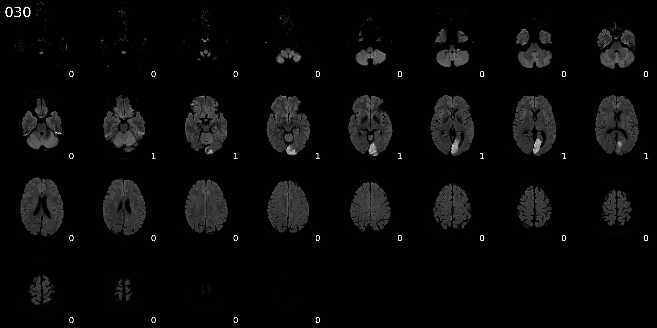
Figure 3: A pseudo 3D diffusion weighted image of an example stroke patient. 2D slices where a stroke lesion is visible are labeled with a 1 and 0 otherwise. Each patient is represented by 28 diffusion weighted images (DWIs) after pre-processing. Ischemic stroke lesions appear as hyper-intense signal on one or multiple images of a sequence.

2.3 Experimental setup

Models

We compare models with varying degrees of interpretability and flexibility for ordinal mRS prediction (see Tab. 1). The goal is to obtain a model which achieves the highest possible prediction power while being adequately interpretable. In all models we choose $F_{Z}(z)=\operatorname{expit}(z)$, such that shift parameters in $h$ can be interpreted as log odds-ratios. By comparing models based on tabular data, image data and a combination of both, we assess if tabular and image data carry complementary information and which of the two contains more information for outcome prediction. As a baseline benchmark, we consider performance metrics of an unconditional model, which takes no input data and hence consists of a simple intercept (SI) only. This model predicts the prevalence of each outcome class. To assess binary mRS prediction, we consider the outcome as censored and sum up the predicted probabilities of the respective ordinal model. The probability for a favorable outcome is the sum across the probabilities for classes 0 to 2, the probability for unfavorable outcome is the sum across the probabilities for classes 3 to 6.

Table 1: Summary of all models used for binary and ordinal functional outcome prediction in the stroke data. If applicable, the transformation function is given. The model names are combinations of the components (simple/complex intercept/shift), the subscript indicates which modality enters which component, where e.g., LS${}_{\text{\boldmath$x$}}$ indicates that the tabular data is the input. SI: Simple intercept. CI: Complex intercept. LS: Linear shift. CS: Complex shift. Note that LS${}_{\text{\boldmath$x$}}$ includes all predictors, including pre-stroke mRS, whereas LS_mRS contains pre-stroke mRS only.

Outcome	Input data	Model name	Transformation function
Binary mRS	Images only	CIB-Binary	$\theta(\mathsf{B})$
Ordinal mRS	None	SI	$\theta_{k}$
	Tabular only	SI-LS${}_{\text{\boldmath$x$}}$	$\theta_{k}-\text{\boldmath$x$}^{\top}\text{\boldmath$\beta$}$
	Tabular only	SI-CSage-LS${}_{\tilde{\text{\boldmath$x$}}}$	$\theta_{k}-\gamma(\text{\boldmath$x$}_{\text{age}})-\text{\boldmath$x$}_{-\text{age}}^{\top}\text{\boldmath$\beta$}$
	Images only	SI-CSB	$\theta_{k}-\eta(\mathsf{B})$
	Images + tabular	SI-CSB-LS${}_{\text{\boldmath$x$}}$	$\theta_{k}-\eta(\mathsf{B})-\text{\boldmath$x$}^{\top}\text{\boldmath$\beta$}$
	Images + pre-stroke mRS	CIB-LS${}_{\text{mRS}}$	$\theta_{k}(\mathsf{B})-\text{\boldmath$x$}_{\text{mRS}}^{\top}\text{\boldmath$\beta$}$
	Images + tabular	CIB-LS${}_{\text{\boldmath$x$}}$	$\theta_{k}(\mathsf{B})-\text{\boldmath$x$}^{\top}\text{\boldmath$\beta$}$
	Tabular only	GAM	$\theta_{k}-\gamma(\text{age})-\text{\boldmath$x$}_{-\text{age}}^{\top}\text{\boldmath$\beta$}$
	Images only	CIB

We define an image-only model which is fitted using the binary mRS (CI_B-Binary in Tab. 1). This dichotomized version of the mRS can be viewed as a censored version of the ordinal mRS and can therefore be directly compared to all models fitted on the ordinal scale (see Tab. 1). We fit the CI_B-Binary model primarily as a benchmark for the performance of the models that are trained for the ordinal but evaluated for the binary mRS.

The most interpretable model for the ordinal mRS is a linear proportional odds model based on all tabular features. It consists of a simple intercept and a linear shift in $x$ (SI-LS${}_{\text{\boldmath$x$}}$). The SI-CS${}_{\texttt{age}}$-LS${}_{\tilde{\text{\boldmath$x$}}}$ model allows the outcome to depend on age in a non-linear way by estimating a potentially complex and continuous log odds-ratio function $x_{\text{age}}$. We additionally fit models depending on image data only (SI-CS_B, CI_B) and on a combination of image and tabular data (SI-CS_B-LS${}_{\text{\boldmath$x$}}$ and CI_B-LS${}_{\text{\boldmath$x$}}$ models). Integrating the images as complex intercept (CI_B) rather than as complex shift term (CS_B) allows to increase model complexity further. In the image model CI_B-LS${}_{\text{mRS}}$, we additionally adjust for the pre-stroke mRS to achieve a fairer comparison between image-data-only and tabular-data-only.

Implementation

Simple intercept and linear shift terms for tabular features are modelled with fully connected NNs without hidden layers. A fully connected NN with multiple hidden layers is used to integrate age as complex shift term. The complex intercept and complex shift terms for the images are modelled with a 3D CNN. In all models, the number of output nodes is equal to six (since the mRS has seven levels) in NNs for intercept terms and equal to one in NNs for shift terms. The last layer activation is always linear and no bias terms are used.

All models are trained by minimizing the negative log-likelihood (see Eq. 1) using the Adam optimizer (Kingma and Ba, 2015) with a learning rate of $5\times 10^{-5}$ and a batch size of six. Augmentation of the image data is used to prevent overfitting. In addition, we use early stopping, i.e., we select the model weights from the epoch which shows the smallest NLL on the validation data. More details on NN architectures, hyperparameters, augmentation procedure and software is given in Appendix A.

Training and evaluation

We randomly split the data six times into a train (80%), validation (10%) and test set (10%). This results in six fits for each model type (see table 1) which allows us to assess the variation of the achieved test performance (see for example Fig. 4 A). For all models, that include the image data as input, we perform transformation ensembling (Kook et al., 2022a). For that, we train five models on the same data in each split. CNNs controlling the image term in the model are initialized randomly. Additional SI and LS${}_{\text{\boldmath$x$}}$ terms are initialized with the corresponding parameters of the SI-LS${}_{\text{\boldmath$x$}}$ model fitted on the same split. This results in an ensemble model (constructed from 5 members) in each of the six splits for each model type.

Performance Measures

All models are mainly evaluated with proper scoring rules (Gneiting and Raftery, 2007). The score we consider primarily for model comparison is the test negative log-likelihood (NLL, Good, 1952, a.k.a. log-score). We further assess the Brier score for the binary outcome. For the ordinal functional outcome, we calculate the ranked probability score as an additional proper score (Bröcker and Smith, 2007). As measures of discriminatory ability, we compute AUC and accuracy for binary outcomes and quadratic weighted Cohen’s $\kappa$ for the ordinal outcome (Steyerberg, 2019). We construct 95% bootstrap confidence intervals by taking $B=1^{\prime}000$ bootstrap samples of size $n_{\rm test}$ of test predictions (e.g., NLL contributions) for each of the $S=6$ random splits of the data, by computing the 2.5th, 50th, and 97.5th percentile of the $B$ bootstrap metrics averaged over the $S$ splits.

3 Results and discussion

We first present results for predicting and discriminating binary and ordinal mRS. Then, we discuss how to interpret linear and non-linear model components.

Binary mRS prediction

The test performance and calibration plots of all models from Tab. 1 evaluated for the binary mRS are summarized in Fig. 4.

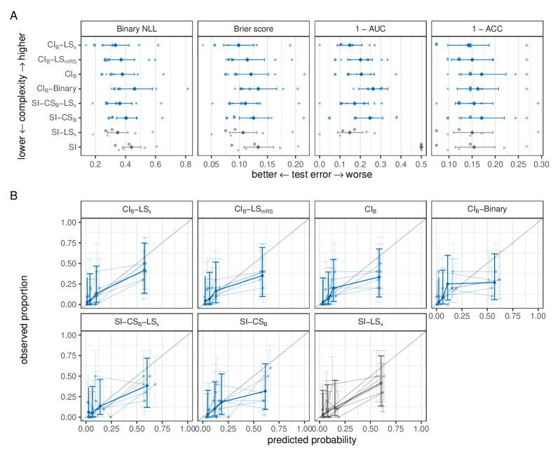
Figure 4: Test error (A) and calibration plots (B) of transformation ensembles (blue) and reference models (grey) evaluated for the binary mRS outcome (mRS 0–2 vs. mRS 3–6). In A, the test performance is quantified in terms of negative log-likelihood (NLL), Brier score, discrimination error ($1-\operatorname{AUC}$) and classification error ($1-\operatorname{ACC}$). From the test performance in the six random splits (indicated by different symbols) we consider the average test error and 95% bootstrap ($B=1^{\prime}000$) confidence intervals. For the calibration plots in B, the predicted probabilities are split at the 0.25, 0.5 and 0.75 empirical quantiles to produce the four bins for which the average predicted probabilities and the observed proportion of an unfavorable outcome are computed. The confidence interval is plotted at the midpoint of the respective bin. Average calibration across all six random splits are shown as thick line whereas the calibration of the single splits are shown as thin lines.

We first compare models which only include the image modality and only differ in the number of classes (CI_B-Binary trained with two vs. CI_B trained with seven classes). The CI_B-Binary model shows a worse average performance and a higher variability in predictions across the six random splits compared to the CI_B. This highlights the importance for training with all available class levels rather than with a dichotomized version of the outcome – whenever possible. The average performance of the CI_B-Binary is similar to that of the unconditional model (SI) indicating that the model has primarily learned the class frequencies. Decreasing model complexity by modelling the image data with a complex shift (SI-CS_B) rather than with a complex intercept (CI_B) leads to a comparable performance. Both models, SI-CS_B and CI_B, achieve a better average prediction performance than the unconditional model (SI) indicating that the image data contains information for mRS binary prediction.

The most interpretable model based on tabular features only (SI-LS${}_{\text{\boldmath$x$}}$) shows a better prediction performance than all models based on image data only (CI_B, CI_B-Binary, SI-CS_B) in terms of NLL and Brier Score. Like the models based on image data only, the SI-LS${}_{\text{\boldmath$x$}}$ outperforms the unconditional model (SI, Fig. 4). This indicates that not only image but also tabular data is useful for binary mRS prediction. For a fairer comparison of image-data-only vs. tabular-data-only, we adjust for pre-stroke mRS in the most flexible image model. In this comparison, the baseline adjusted model (CI_B-LS_mRS) shows a performance similar to the unadjusted model (CI_B).

The semi-structured models incorporating both image and tabular data (CI_B-LS${}_{\text{\boldmath$x$}}$and SI-CS_B-LS${}_{\text{\boldmath$x$}}$) achieve a similar or slightly better average performance than the model including tabular data only (SI-LS${}_{\text{\boldmath$x$}}$, see Fig. 4). CI_B-LS${}_{\text{\boldmath$x$}}$does not assume proportional odds for the image modality and outperforms SI-CS_B-LS${}_{\text{\boldmath$x$}}$on some splits. The latter assumes proportional odds for both tabular and image data. Overall, there is no convincing evidence that combining tabular and imaging data in a CI_B-LS${}_{\text{\boldmath$x$}}$model improves binary mRS prediction. The added image information increases variability in prediction performance.

Scores highlighting discriminatory ability of the models (AUC and accuracy) show similar results. Slight differences in the ranking of models are possible because these measures are improper scoring rules (Gneiting and Raftery, 2007). Note that SI has no discriminatory ability (AUC $=$ 0.5) because it always predicts the most frequent class (mRS 0). The relative test performance to the benchmark SI-LS${}_{\text{\boldmath$x$}}$ model (i.e., the differences in performance within splits) can be found in Appendix B.2.

Well-calibrated predictions are hard to achieve for highly imbalanced outcomes. The calibration plots in Fig. 4 show no substantial evidence for miscalibration. However, all models seem to slightly over-predict the probability for an unfavorable outcome. This effect is most pronounced in the models based on image data only (CI_B, CI_B-Binary). The semi-structured and tabular data-only models show a slightly better calibration.

Ordinal mRS prediction

Fig. 5 summarizes the test performance and calibration plots for all models in Tab. 1 trained and evaluated for the ordinal mRS.

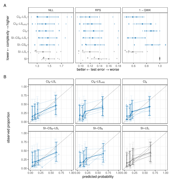
Figure 5: Test error (A) and calibration plots (B) of transformation ensembles (blue) and reference models (grey) evaluated for the ordinal mRS outcome. In A, test error is quantified in terms of negative log-likelihood (NLL), ranked probability score (RPS), and discrimination error ($1-\operatorname{QWK}$). The average test error and 95% bootstrap ($B=1^{\prime}000$) confidence intervals are depicted for six random splits of the data (indicated by the different symbols). For the calibration plots in B, the predicted probabilities are split at the 0.25, 0.5 and 0.75 empirical quantiles to produce the four bins for which the average predicted probabilities and the observed proportion of an unfavorable outcome are computed. The confidence interval is plotted at the midpoint of the respective bin. Average calibration across all six random splits is shown as thick line whereas the calibration of the single splits is shown as thin lines. 95% confidence intervals are averaged across classes and splits.

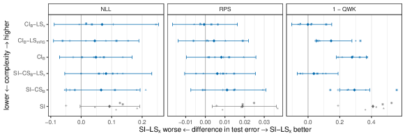
Figure B3: Test error of transformation ensemble models (blue) and reference model (grey) evaluated for the ordinal mRS outcome relative to the test error of the benchmark SI-LS${}_{\text{\boldmath$x$}}$ model (i.e., a difference of 0 indicates the same performance as the SI-LS${}_{\text{\boldmath$x$}}$ model). The test error is quantified in terms of negative log-likelihood (NLL), ranked probability score (RPS) and discrimination error ($1-\operatorname{QWK}$). The average test error and 95% bootstrap ($B=1^{\prime}000$) confidence intervals (CI) are depicted for six random splits (indicated by different symbols). The CIs are calculated by substracting the fixed SI-LS${}_{\text{\boldmath$x$}}$ performance per split.

As in the binary case, the models based on image (CI_B, SI-CS_B) and tabular data only (SI-LS${}_{\text{\boldmath$x$}}$) show better average prediction performances in terms of NLL, RPS and QWK than the unconditional model (SI). And again, the most interpretable model based on tabular data only (SI-LS${}_{\text{\boldmath$x$}}$) outperforms the more flexible black box image-only models, indicating that tabular features contain more information for ordinal mRS prediction than the images (at the available sample with only 407 patients). As in the binary case, we find no substantial evidence that using tabular and image data together in a semi-structured model (CI_B-LS${}_{\text{\boldmath$x$}}$, CI_B-LS_mRS or SI-CS_B-LS${}_{\text{\boldmath$x$}}$) improves average test performance compared to SI-LS${}_{\text{\boldmath$x$}}$ (see Fig. B3).

In terms of calibration (Fig. 5B) we again observe that all models over-predicted the probability for an unfavorable outcome.

Overall, we can not draw a definitive conclusion about which data modality (tabular or image data) is more useful for functional outcome prediction and if adding image to tabular data aids mRS prediction. The confidence intervals overlap largely and average test performance is similar. In particular, this can be attributed to the small sample size. In Appendix B.3, we conclude that collecting more data could further enhance performance. When we artificially reduce sample size via sub-sampling and refit all models, we find no evidence of plateauing prediction performance. However, no differential increase in prediction performance is observed for the tabular-data-only model compared to the most complex DTM.

Interpretation of model parameters

Fig. 6 visualizes the effect sizes of the tabular features in the linear shift terms LS${}_{\text{\boldmath$x$}}$ of different models.

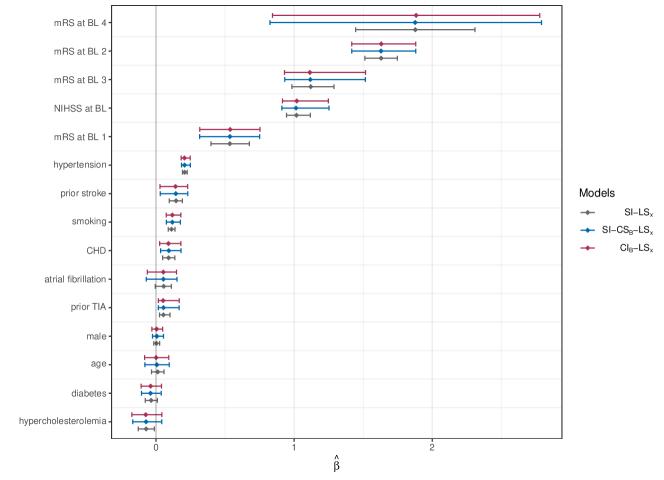
Figure 6: Pooled log odds-ratios ($\hat{\text{\boldmath$\beta$}}$) across all six random splits and 95% bootstrap ($B=1^{\prime}000$) confidence intervals for all models with linearly included tabular features (see Section 2.2). With the exception of age and NIHSS, all features are categorical and the plot shows log odds-ratios with respect to the reference level (note that the largest observed pre-stroke mRS is 4). The coefficients are based on standardized features and sorted with respect to an increasing order.

Because the logistic distribution is chosen for $Z$, the coefficients $\beta$ in the linear shift term are interpretable as log odds-ratios. Comparing tabular-data-only models with semi-structured models shows that adjusting for the images (in CI_B-LS${}_{\text{\boldmath$x$}}$ or SI-CS_B-LS${}_{\text{\boldmath$x$}}$) changes the $\hat{\text{\boldmath$\beta$}}$ estimates only slightly. The log odds-ratios are comparable across all variables because the variables are standardized. Thus, the effect sizes reflect a change in log-odds of a worse outcome for a one standard deviation increase in the respective variable. Accordingly, Fig. 6 shows that the strongest prognostic factors are the pre-stroke mRS and NIHSS on admission. This is expected when predicting three months mRS. The pre-stroke mRS captures functional disability of a patient before stroke while NIHSS measures stroke severity on admission. This additionally emphasizes the importance for being able to adjust for pre-stroke mRS.

Similar to both linear and complex shift terms, complex intercepts of categorical predictors are directly interpretable. Here, cumulative baseline log-odds of the outcome are estimated for each stratum of the predictor. Thus, differences in the complex intercepts can be interpreted as class-specific log-odds ratios (Buri et al., 2020). For continuous predictors or images, this simple interpretation is lost to an extent which depends on the complexity of the neural network component that is modelling the complex intercept term.

Alongside interpretation, quantifying uncertainty in both predictions and parameters is of high importance, but generally difficult to achieve in deep learning models (Wilson and Izmailov, 2020). The use of transformation ensembles and random splits allows uncertainty quantification for the coefficient estimates in terms of bootstrap confidence intervals. This way, both aleatoric and epistemic uncertainty are captured. Note, that the model coefficients of the five (members) times six (splits) are repeatedly sampled and that the models are not additionally refitted to obtain the 95% confidence intervals.

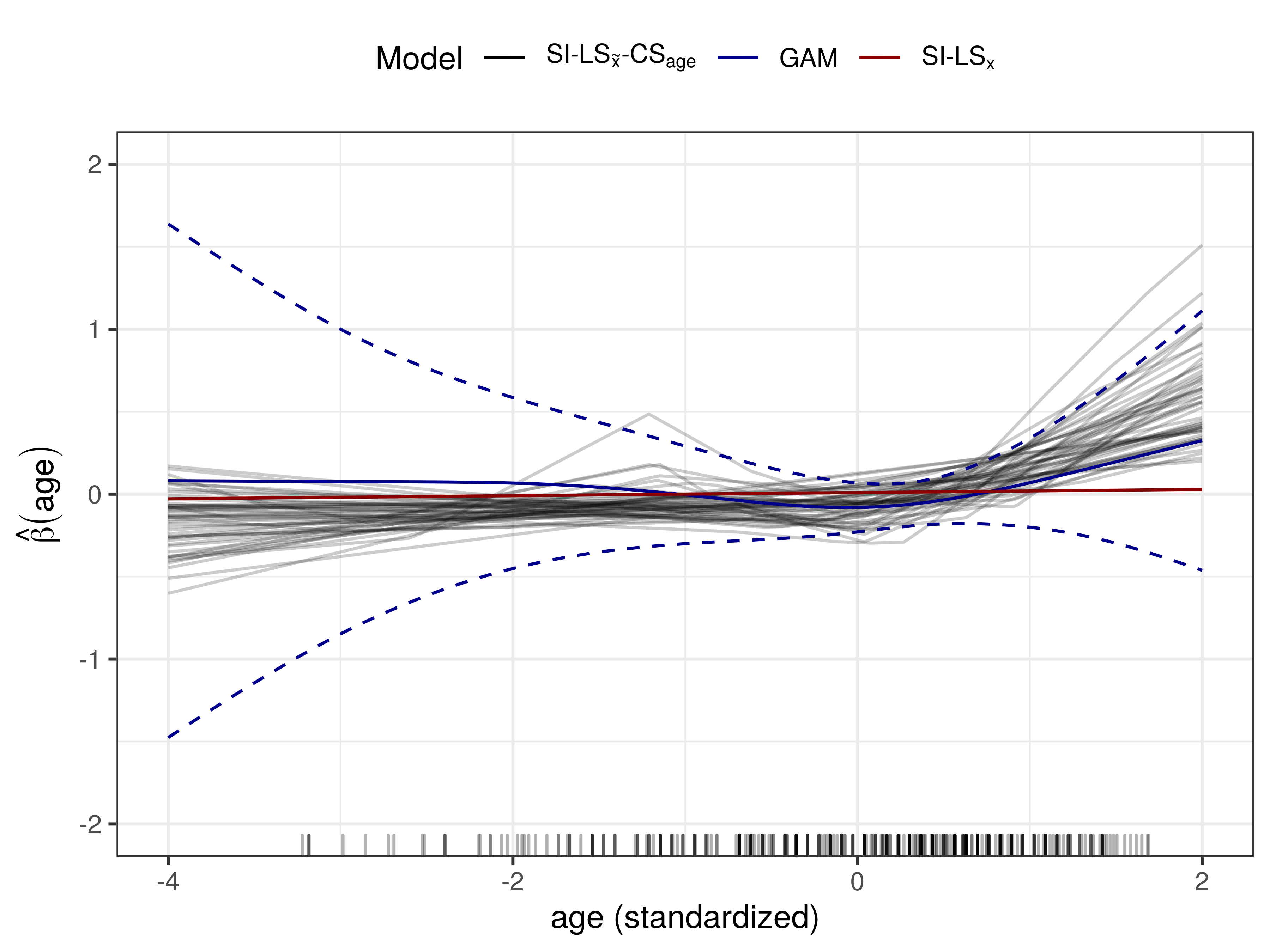
Figure 7: The smooth log-odds function for age fitted by a GAM (a generalized additive proportional odds model using the mgcv package), depicted as blue solid line along with point-wise 95% confidence band (dashed lines), and by a DTM (SI-LS${}_{\tilde{\text{\boldmath$x$}}}$-CS_age) fitted on 50 bootstrap samples, depicted as grey lines. In addition, the linear effect of a SI-LS${}_{\text{\boldmath$x$}}$ is displayed (red line). Although both models, GAM and DTM, allow for a non-linear effect in age, there is no evidence against a linear effect of age.

To investigate if assuming a linear age effect is appropriate, we evaluate models including the age effect with a flexible function, $\theta_{k}-\gamma(x_{\text{age}})-\text{\boldmath$x$}_{-\text{age}}^{\top}\text{\boldmath$\beta$}$. We show the results of a GAM (a generalized additive proportional odds model) and a DTM (SI-LS${}_{\text{\boldmath$x$}}$-CS_age) which depict the estimated age effect function as shown in Fig. 7. The GAM and the DTM agree in the functional form of the effect, which is constant up to a standardized age of 0.5 (corresponding to an age of 75 years) and then increases the odds for a worse outcome. However, there is no evidence against a linear effect when we consider the point-wise confidence band for the GAM. Note how the GAM enforces smoothness of the estimated function, whereas the neural network produces a piece-wise linear estimate.

4 Summary and outlook

DTMs provide a novel and flexible way to integrate multi-modal data for interpretable prediction models for various kinds of outcomes. We demonstrate the potential of DTMs on a semi-structured data set with an ordinal outcome (mRS) describing the functional disability of stroke patients three months after hospital admission. We discuss how the best trade-off between interpretability and flexibility can be achieved. In essence, we follow the top-down model approach to model building for TMs (Hothorn, 2018). By investigating the interpretable model parameters, we judge the relative importance of the predictors and show that in a baseline-adjusted DTMs, the base-line mRS is the variable with the most relevant predictive effect. We also investigate the question, which input modality is most important for functional outcome prediction and whether predictive performance in terms of NLL and calibration can be improved by including both tabular and imaging data. While for binary mRS prediction, models seemed to slightly benefit from the addition of brain imaging data, this is not observed for ordinal mRS prediction. In general, a definitive judgement on whether the images contain information to aid mRS prediction cannot be made. This is because, all results have to be interpreted conditional on (i) the small sample size and (ii) limited computation time for joint hyper-parameter tuning. When artificially increasing the sample size up to the available 407 patients, there is no evidence for differential performance gain of the semi-structured over tabular-data-only models. However, extrapolating these results to larger sample sizes is in general extremely difficult.

In general, deep neural networks (including DTMs) are difficult to train with limited sample size and require a carefully chosen optimization procedure. For instance, transfer learning in terms of adapting the weights of a CNN that is already trained on a different data set by re-training it with the data of interest potentially improves predictive performance even with smaller sample sizes. However, methods for transferring the weights of well-known 2D CNN architectures to their 3D counterparts did not improve predictive performance in our application (results not shown). In general, it is difficult to access weights of trained 3D CNNs to then fine-tune the models.

For ordinal functional outcome prediction in our cohort, the model SI-LS${}_{\text{\boldmath$x$}}$ seemed to be most appropriate when including tabular features only and modelling them as linear effects. Here, classical statistical inference provides uncertainty measures (confidence intervals) and the model is fully interpretable. Using semi-structured models, including tabular and brain imaging data, improved binary mRS prediction to some extent. However, including images as a complex intercept or complex shift reduced interpretability of the model and increased variability.

TMs also work naturally for other kinds of outcomes, such as survival times, which often feature censored observations (e.g.,  Hothorn et al., 2018). Because the dichotomized mRS could be viewed as a censored version of the ordinal mRS, the very same models, trained on ordinal outcomes, can also be used for different dichotimizations (or binnings) of the ordinal outcome, without the need to re-fit the models on the binned outcome (Lohse et al., 2017).

In summary, being able to fit distributional regression models with complex outcome types and multi-modal input data and following statistical principles for model building opens up vast areas of applications. Especially in medicine, these models have the potential to aid decision making, because of their state-of-the-art prediction performance and transparency.

Appendix A Computational details

For reproducibility, all code is made publicly available on GitHub https://www.github.com/LucasKookUZH/dtm-usz-stroke.

Neural Network architectures

The simple intercept terms are modelled with a fully connected single-layer NN without hidden layers and linear activation. No bias term is used. The number of output nodes is always equal to the number of classes minus one while the input is a vector of ones.

The linear shift terms for the tabular data are modelled with fully connected NNs without hidden layers and a linear function as activation. No bias term is used. The number of input units is equal to the number of tabular features while the number of units in the last layer is equal to one.

The complex shift term for the variable age is modelled with a fully connected NN with two hidden layers with 16 units each, ReLU activation function and $L_{2}$ regularization. The number of units in the last layer is equal to one and the activation function in this layer is linear.

The complex intercept and complex shift terms for the image data are modelled with a 3D CNN. The convolutional part of the 3D CNN consists of four convolutional blocks including a convolutional layer with filter size $3\times 3\times 3$ and a max pooling layer of size $2\times 2\times 2$. The first two layers use 32 filters, the following two use 64 filters. The subsequent fully connected part consists of two fully connected layers with 128 filters each, that are separated by a dropout layer with dropout rate 0.3. The activation function in all layers, expect the last one, is the ReLU non-linearity. In case the image data is included as complex intercept term, the number of units in the last layer is equal to the number of classes minus one, i.e., one when we predict the binary mRS and 6 when we predict the ordinal mRS. When integrated as complex shift term, the number of units in the last layer is equal to one. The activation function in the last layer is linear.

Training

All models are fitted with stochastic gradient descent using the Adam optimizer [Kingma and Ba, 2015] with a learning rate of $5\times 10^{-5}$ and a batch size of six. We then use the model with the best performance on the validation data in terms of NLL. For all experiments, the 3D images were augmented in x- and y-direction prior to every epoch using the parameters in Tab. A1.

Table A1: Parameter values for augmentation.

Parameter	Value
rotation range	20
width shift range	0.2
height shift range	0.2
shear range	0.15
zoom range	0.15
fill	nearest

All models are implemented in R 4.1.2 [R Core Team, 2020]. The models are written in Keras based on TensorFlow backend using TensorFlow version 2.2.0 [Chollet et al., 2015, Abadi et al., 2015] and trained on a GPU. Linear proportional odds models and generalized additive proportional odds models are fitted using tram::Polr [Hothorn, 2020] and mgcv::gam [Wood, 2017], respectively.

Appendix B Additional results

Here, we present descriptive statistics and additional results.

B.1 Baseline characteristics

Fig. B1 shows the distribution of predictors stratified by the outcome (90 day mRS) in the stroke data set.

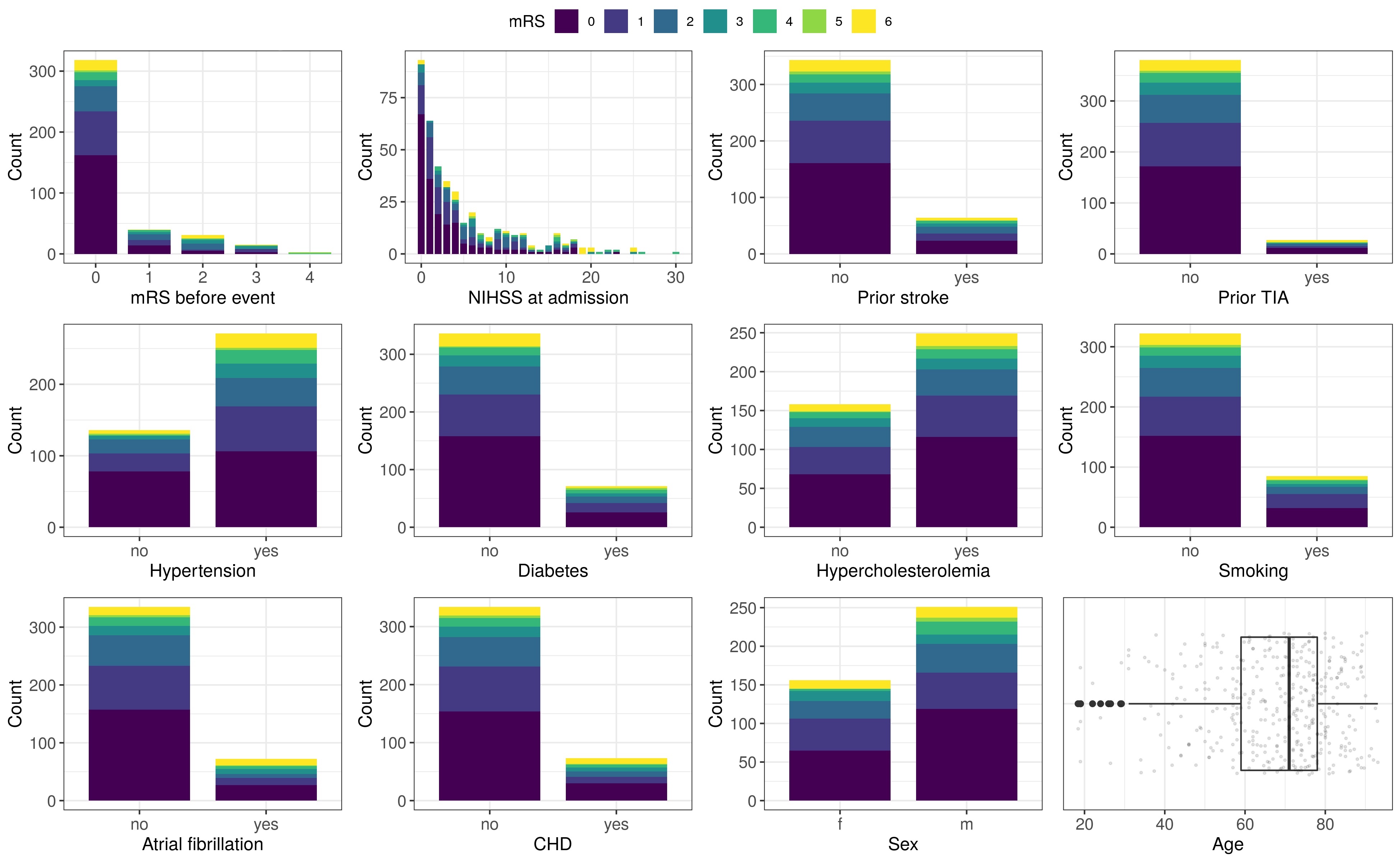
Figure B1: Baseline characteristics stratified by 90 day mRS in the stroke data set.

B.2 Test errors relative to reference model

Figg. B2 and B3 show the test errors relative to the reference SI-LS${}_{\text{\boldmath$x$}}$ model evaluated on the binary and ordinal mRS, respectively. After removing the between-split variance, none of the semi-structured models improve significantly upon the performance of the SI-LS${}_{\text{\boldmath$x$}}$ model. Since the SI-LS${}_{\text{\boldmath$x$}}$ performance was not bootstrapped (the constant split-wise mean was subtracted within split) there is no variance in the average AUC and QWK (because the SImodel does not have any discriminatory ability, i.e., AUC $=0.5$ and QWK $=0$) across splits for the unconditional SI model.

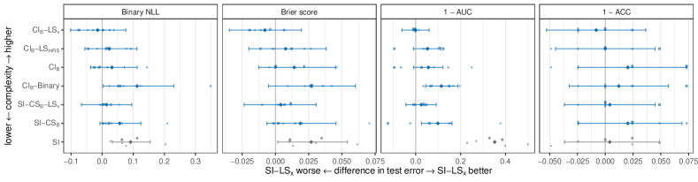
Figure B2: Test error of transformation ensemble models (blue) and reference model (grey) evaluated for the binary mRS outcome (mRS 0–2 vs. mRS 3–6) relative to the test error of the benchmark SI-LS${}_{\text{\boldmath$x$}}$ model (i.e., a difference of 0 indicates the same performance as the SI-LS${}_{\text{\boldmath$x$}}$ model). The test error is quantified in terms of binary negative log-likelihood (NLL), Brier score, $1-$ area under the ROC curve (AUC) and classification error ($1-\operatorname{ACC}$). The average test error and 95% bootstrap ($B=1^{\prime}000$) confidence intervals (CI) are depicted for six random splits (indicated by different symbols). The CIs are calculated by substracting the fixed SI-LS${}_{\text{\boldmath$x$}}$ performance per split.

B.3 Sample size

Deep learning typically requires thousands of training images to excel at prediction performance over conventional statistical models [Goodfellow et al., 2016]. However, our cohort, like most medical data sets, contained much fewer observations ($n=407$). To study if collecting more data was a promising approach to enhance the model performance, we artificially reduced sample size by sub-sampling and refitted the models (see Fig. B4).

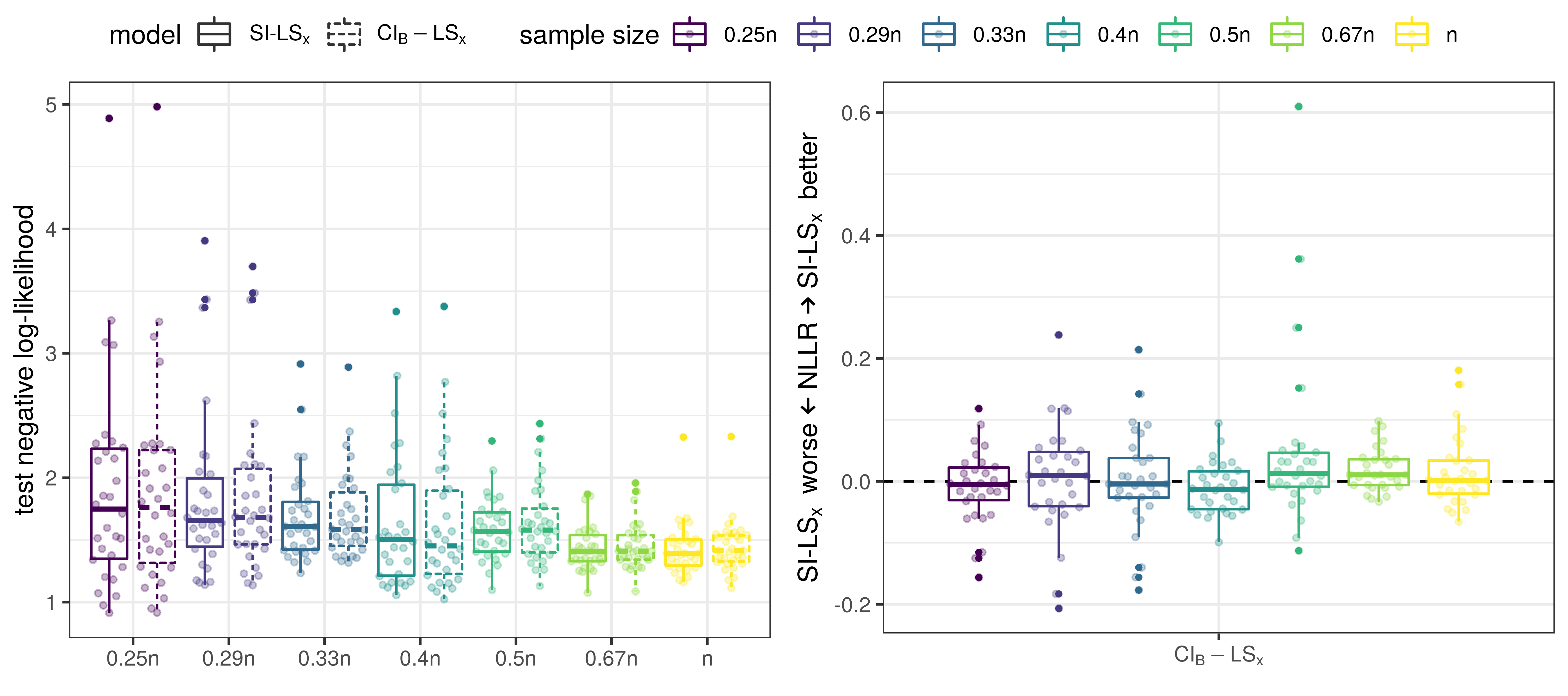
Figure B4: Test performance versus sample size achieved by a subsampling experiment. The semi-structured CI_B-LS${}_{\text{\boldmath$x$}}$ model and the proportional odds model SI-LS${}_{\text{\boldmath$x$}}$ are compared. Both models are fitted to 30 random sub-samples of seven different sample sizes of the original sample size ($n=407$) and the test NLL is recorded. Both models benefit from increasing sample size. The right panel displays the differences in NLL within split for a given sample size (i.e., the negative log-likelihood ratio NLLR).

In this experiment, the sample size is artificially reduced via sub-sampling of varying sizes and then the prediction performance was measured on a hold-out set of the reduced data set. Sub-sampling is repeated for seven sample sizes and then 30 train/validation/test splits (with a ratio of 8:1:1) are used for fitting and evaluating the semi-structured CI_B-LS${}_{\text{\boldmath$x$}}$ and tabular-data-only model SI-LS${}_{\text{\boldmath$x$}}$. We observe that the prediction performance, i.e., the test NLL, improves for both models with increasing sample size, indicating that the performance may further increase with increasing sample size (left panel of Fig. B4). Directly comparing the performance of both models for the individual splits suggests no evidence that adding the image information to the model that contained the tabular data as input improves prediction performance. The negative log-likelihood ratio fluctuates around zero and no trend with increasing sample size is observable (right panel in Fig. B4).

References

- Abadi et al. [2015] Martín Abadi et al. TensorFlow: Large-scale machine learning on heterogeneous systems, 2015. URL http://tensorflow.org/. Software available from tensorflow.org.
- Bacchi et al. [2020] Stephen Bacchi, Toby Zerner, Luke Oakden-Rayner, Timothy Kleinig, Sandy Patel, and Jim Jannes. Deep learning in the prediction of ischaemic stroke thrombolysis functional outcomes: A pilot study. Acadamic Radiology, 27:19–23, 2020. doi: 10.1016/j.acra.2019.03.015.
- Baumann et al. [2021] Philipp F. M. Baumann, Torsten Hothorn, and David Rügamer. Deep conditional transformation models. In Machine Learning and Knowledge Discovery in Databases. Research Track, pages 3–18. Springer International Publishing, 2021. doi: 10.1007/978-3-030-86523-8_1.
- Benjamine et al. [2019] Emelia J. Benjamine, Paul Muntner, Alvaro Alonso, Marcio S. Bittencourt, Clifton W. Callaway, April P. Carson, Alanna M. Chamberlain, Alexander R. Chang, Susan Cheng, et al. Heart Disease and Stroke Statistics – 2019 Update: A Report From the American Heart Association. Circulation, 139(10):56–528, 2019. doi: 10.1161/CIR.0000000000000659.
- Bröcker and Smith [2007] Jochen Bröcker and Leonard A Smith. Scoring probabilistic forecasts: The importance of being proper. Weather and Forecasting, 22(2):382–388, 2007. doi: 10.1175/WAF966.1.
- Buri et al. [2020] Muriel Buri, Armin Curt, John Steeves, and Torsten Hothorn. Baseline-adjusted proportional odds models for the quantification of treatment effects in trials with ordinal sum score outcomes. BMC Medical Research Methodology, 20(1), 2020. doi: 10.1186/s12874-020-00984-2.
- Campanella et al. [2019] Gabriele Campanella, Matthew G. Hanna, Luke Geneslaw, Allen Miraflor, Vitor Werneck Krauss Silva, Klaus J. Busam, Edi Brogi, Victor E. Reuter, David S. Klimstra, and Thomas J. Fuchs. Clinical-grade computational pathology using weakly supervised deep learning on whole slide images. Nature Medicine, 25(8):1301–1309, 2019. doi: 10.1038/s41591-019-0508-1.
- Chollet et al. [2015] François Chollet et al. Keras. https://keras.io, 2015.
- Copen et al. [2011] William A. Copen, Pamela W. Schaefer, and Ona Wu. Mr perfusion imaging in acute ischemic stroke. Neuroimaging Clinics of North America, 21:259–283, 05 2011. doi: 10.1016/j.nic.2011.02.007.
- Ebisu et al. [1997] Toshihiko Ebisu, Chuzo Tanaka, Masahiro Umeda, Makoto Kitamura, Masaki Fukunaga, Ichiro Aoki, Hiroshi Sato, Toshihiro Higuchi, Shoji Naruse, Yoshiharu Horikawa, et al. Hemorrhagic and nonhemorrhagic stroke: diagnosis with diffusion-weighted and t2-weighted echo-planar mr imaging. Radiology, 203(3):823–828, 1997. doi: 10.1148/radiology.203.3.9169711.
- Gneiting and Raftery [2007] Tilmann Gneiting and Adrian E Raftery. Strictly proper scoring rules, prediction, and estimation. Journal of the American Statistical Association, 102(477):359–378, 2007. doi: 10.1198/016214506000001437.
- Good [1952] I. J. Good. Rational decisions. Journal of the Royal Statistical Society. Series B (Statistical Methodology), 14(1):107–114, 1952. doi: 10.1111/j.2517-6161.1952.tb00104.x.
- Goodfellow et al. [2016] Ian Goodfellow, Yoshua Bengio, and Aaron Courville. Deep Learning. MIT press, 2016. doi: 10.1007/s10710-017-9314-z.
- Grotta et al. [2016] James C. Grotta, Gregory W. Albers, Joseph P. Broderick, Scott E. Kasner, Eng H. Lo, A. David Mendelow, Ralph L. Sacco, and Lawrence K.S. Wong. Stroke: Pathophysiology, Diagnosis, and Management. Elsevier, 6 edition, 2016.
- Hamann & Herzog et al. [2021] Janne Lisa Hamann & Herzog, Carina Wehrli, Tomas Dobrocky, Andrea Bink, Marco Piccirelli, Leonidas Panos, Johannes Kaesmacher, Urs Fischer, Christoph Stippich, Jan Luft, Andreas R. Gralla, Marcel Arnold, Roland Wiest, Beate Sick, and Susanne Wegener. Machine-learning based outcome prediction in stroke patients with middle cerebral artery-m1 occlusions and early thrombectomy. European Journal of Neurology, 28:1234–1243, 2021. doi: 10.1111/ene.14651.
- Hothorn [2018] Torsten Hothorn. Top-down transformation choice. Statistical Modelling, 18(3-4):274–298, 2018. doi: 10.1177/1471082X17748081.
- Hothorn [2020] Torsten Hothorn. tram: Transformation Models, 2020. URL https://CRAN.R-project.org/package=tram. R package version 0.5-1.
- Hothorn et al. [2014] Torsten Hothorn, Thomas Kneib, and Peter Bühlmann. Conditional transformation models. Journal of the Royal Statistical Society. Series B (Statistical Methodology), 76(1):3–27, 2014. doi: 10.1111/rssb.12017.
- Hothorn et al. [2018] Torsten Hothorn, Lisa Möst, and Peter Bühlmann. Most Likely Transformations. Scandinavian Journal of Statistics, 45(1):110–134, 2018. doi: 10.1111/sjos.12291.
- Jafari et al. [2018] Seyed Hamed Jafari, Zahra Saadatpour, Arash Salmaninejad, Fatemeh Momeni, Mojgan Mokhtari, Javid Sadri Nahand, Majid Rahmati, Hamed Mirzaei, and Mojtaba Kianmehr. Breast cancer diagnosis: Imaging techniques and biochemical markers. Journal of Cellular Physiology, 233(7):5200–5213, 2018. doi: 10.1002/jcp.26379.
- Kingma and Ba [2015] Diederik P. Kingma and Jimmy Lei Ba. Adam: A method for stochastic optimization. In 3rd International Conference on Learning Representations, ICLR 2015 - Conference Track Proceedings. International Conference on Learning Representations, ICLR, 2015. URL https://arxiv.org/abs/1412.6980v9.
- Kneib et al. [2021] Thomas Kneib, Alexander Silbersdorff, and Benjamin Säfken. Rage against the mean–a review of distributional regression approaches. Econometrics and Statistics, 2021. doi: 10.1016/j.ecosta.2021.07.006.
- Kook et al. [2022a] Lucas Kook, Andrea Götschi, Philipp FM Baumann, Torsten Hothorn, and Beate Sick. Deep interpretable ensembles. arXiv preprint, 2022a. doi: 10.48550/arxiv.2205.12729.
- Kook et al. [2022b] Lucas Kook, Lisa Herzog, Torsten Hothorn, Oliver Dürr, and Beate Sick. Deep and interpretable regression models for ordinal outcomes. Pattern Recognition, 122:108263, February 2022b. doi: 10.1016/j.patcog.2021.108263.
- Lakshminarayanan et al. [2017] Balaji Lakshminarayanan, Alexander Pritzel, and Charles Blundell. Simple and scalable predictive uncertainty estimation using deep ensembles. In Advances in Neural Information Processing Systems, volume 30. Curran Associates, Inc., 2017. URL https://proceedings.neurips.cc/paper/2017/file/9ef2ed4b7fd2c810847ffa5fa85bce38-Paper.pdf.
- Lohse et al. [2017] Tina Lohse, Sabine Rohrmann, David Faeh, and Torsten Hothorn. Continuous outcome logistic regression for analyzing body mass index distributions. F1000Research, 6:1933, 2017. doi: 10.12688/f1000research.12934.1.
- McCullagh [1980] Peter McCullagh. Regression models for ordinal data. Journal of the Royal Statistical Society: Series B (Statistical Methodology), 42(2):109–127, 1980. doi: 10.1111/j.2517-6161.1980.tb01109.x.
- Pinto et al. [2018] Adriano Pinto, Richard McKinley, Victor Alves, Roland Wiest, Carlos A. Silva, and Mauricio Reyes. Stroke lesion outcome prediction based on mri imaging combined with clinical information. Frontiers in Neurology, 9:1060, 2018. doi: 10.3389/fneur.2018.01060.
- Quinn et al. [2009] Terence J Quinn, Jesse Dawson, Matthew Walters, and Kennedy R Lees. Reliability of the modified rankin scale: a systematic review. Stroke, 40(10):3393–3395, 2009. doi: 10.1161/STROKEAHA.109.557256.
- R Core Team [2020] R Core Team. R: A Language and Environment for Statistical Computing. R Foundation for Statistical Computing, Vienna, Austria, 2020. URL https://www.R-project.org/.
- Rezende and Mohamed [2015] Danilo Rezende and Shakir Mohamed. Variational inference with normalizing flows. In International Conference on Machine Learning, pages 1530–1538. PMLR, 2015. URL https://proceedings.mlr.press/v37/rezende15.html.
- Rudin [2019] Cynthia Rudin. Stop explaining black box machine learning models for high stakes decisions and use interpretable models instead. Nature Machine Intelligence, 1(5):206–215, 2019. doi: 10.1038/s42256-019-0048-x.
- Rügamer et al. [2020] David Rügamer, Chris Kolb, and Nadja Klein. A unifying network architecture for semi-structured deep distributional learning. arXiv preprint arXiv:2002.05777, 2020. URL https://arxiv.org/abs/2002.05777.
- Rügamer et al. [2021] David Rügamer, Philipp FM Baumann, Thomas Kneib, and Torsten Hothorn. Transforming autoregression: Interpretable and expressive time series forecast. arXiv preprint at arXiv:2110.08248, 2021. URL https://arxiv.org/abs/2110.08248.
- Sick et al. [2021] Beate Sick, Torsten Hothorn, and Oliver Durr. Deep transformation models: Tackling complex regression problems with neural network based transformation models. In 2020 25th International Conference on Pattern Recognition (ICPR). IEEE, 2021. doi: 10.1109/icpr48806.2021.9413177.
- Siegfried and Hothorn [2020] Sandra Siegfried and Torsten Hothorn. Count transformation models. Methods in Ecology and Evolution, 11(7):818–827, 2020. doi: 10.1111/2041-210X.13383.
- Stasinopoulos and Rigby [2007] D Mikis Stasinopoulos and Robert A Rigby. Generalized additive models for location scale and shape (GAMLSS) inR. Journal of Statistical Software, 23(7), 2007. doi: 10.18637/jss.v023.i07.
- Steyerberg [2019] Ewout W Steyerberg. Clinical Prediction Models. Springer, 2019.
- Thiran and Macq [1996] Jean Philippe Thiran and Benoît Macq. Morphological feature extraction for the classification of digital images of cancerous tissues. In IEEE Transactions on Biomedical Engineering, volume 43, pages 1011–1020. Institute of Electrical and Electronics Engineers (IEEE), 1996. doi: 10.1109/10.536902.
- Weisscher et al. [2008] Nadine Weisscher, Marinus Vermeulen, Yvo B Roos, and Rob J De Haan. What should be defined as good outcome in stroke trials; a modified rankin score of 0–1 or 0–2? Journal of Neurology, 255(6):867–874, 2008. doi: 10.1007/s00415-008-0796-8.
- Wilson and Izmailov [2020] Andrew Gordon Wilson and Pavel Izmailov. Bayesian deep learning and a probabilistic perspective of generalization. In Advances in Neural Information Processing Systems (NeurIPS), 2020. URL https://arxiv.org/abs/2002.08791.
- Wood [2017] Simon N Wood. Generalized Additive Models: An Introduction with R. Chapman and Hall/CRC, 2 edition, 2017.