Sharp inequalities involving the Cheeger constant of planar convex sets

Abstract.

We are interested in finding sharp bounds for the Cheeger constant via different geometrical quantities, such as the area $|\cdot|$, the perimeter $P$, the inradius $r$, the circumradius $R$, the minimal width $w$ and the diameter $d$. In particular, we provide new sharp inequalities between these quantities for planar convex bodies and we provide new conjectures based on numerical simulations. In particular, we completely solve the Blasche-Santaló diagrams describing all the possible inequalities involving the Cheeger constant, the perimeter and the inradius, then, the Cheeger constant, the diameter and the inradius, and, finally, the Cheeger constant, the circumradius and the inradius.

Keywords: Cheeger constant, convex sets, Blaschke–Santaló diagrams, sharp inequalities.
MSC 2020: 52A10, 52A40, 65K15.

1. Introduction

Let $\Omega$ be a bounded subset of $\mathbb{R}^{2}$. The Cheeger constant of $\Omega$, introduced by Jeff Cheeger in [27] in connection with the first eigenvalue of the Laplacian, is defined as

(1) $$h(\Omega):=\inf\left\{\frac{P(E)}{{\left|E\right|}}\,:\,E\,\text{measurable and}\,E\subseteq\Omega\right\},$$

where $P(E)$ is the perimeter of $E$ in the sense of De Giorgi and ${\left|E\right|}$ is the area of $E$. The minimum in (1) is achieved when $\Omega$ has Lipschitz boundary, see as a reference [33], and the set $E$ that realizes this minimum is called a Cheeger set of $\Omega$ and it is denoted by $C_{\Omega}$. For the properties of the Cheeger constant and for an introductory survey, see for example [1, 28, 33]. In particular, in the case of planar convex sets, the authors in [1] prove that the Cheeger set is unique, while in [28] the authors give a characterization for the Cheeger constant.

The problem of finding the Cheeger constant of a domain has been widely considered and it has several applications (see [33] for a general overview). One of the possible interpretations of the Cheeger constant can be found for instance in the context of maximal flow and minimal cut problems (see [41]) and this has applications in medical images process (see [4]). The Cheeger problem appears also in the study of plate failure under stress (see [29]). For these reasons, it is useful to have estimates of the Cheeger constant in terms of geometric quantities that can be easily computed.

In the present paper, we are interested in describing all possible inequalities involving the Cheeger constant of a given open, bounded and convex set $\Omega\subset\mathbb{R}^{2}$ and two among the following geometrical quantities: the area ${\left|\Omega\right|}$, the perimeter $P(\Omega)$, the inradius $r(\Omega)$, the circumradius $R(\Omega)$, the minimal width $\omega(\Omega)$ and the diameter $d(\Omega)$. So, we aim to study the associated Blaschke–Santaló diagrams of these triplets and collect them all in one single paper together with new conjectures.

A Blaschke–Santaló diagram is a tool that allows one to visualize all the possible inequalities between three geometric quantities. More precisely, if we consider three shape functionals $(J_{1},J_{2},J_{3})$, we want to find a system of inequalities describing the set

$$\{(J_{1}(\Omega),J_{2}(\Omega))|\ J_{3}(\Omega)=1,\,\Omega\in\mathcal{K}^{2}\},$$

where we denote by $\mathcal{K}^{2}$ the class of non-empty sets in $\mathbb{R}^{2}$ that are open, bounded and convex. This kind of diagram was introduced by Blaschke in [5], in order to investigate all possible relations between the volume, the surface area and the integral mean curvature in the class of compact convex sets in $\mathbb{R}^{3}$. Following the idea of Blaschke, Santaló in [37] proposed the study of these diagrams for all the triplets of the following geometrical quantities: area, perimeter, inradius, circumradius, minimal width and diameter; these diagrams were studied under the constraint of convexity and six of them are still not completely solved. We refer to the introduction in [13] for the accurate state of art. Moreover, for classical results about Blaschke–Santaló diagram, we refer for example to [9, 21, 22, 23, 24, 25, 37] and for more recent results we recall [10, 11, 12, 13, 16, 17, 32].

In [14] and [15] the author studies the Blaschke–Santaló diagram involving the Cheeger constant. More precisely, in [14], it is studied the Blaschke–Santaló diagram between the Cheeger constant, the area and the inradius, and it is proved that, if $\Omega$ in $\mathcal{K}^{2}$, then

(2) $$\frac{1}{r(\Omega)}+\frac{\pi r(\Omega)}{|\Omega|}\leq h(\Omega)\leq\frac{1}{r(\Omega)}+\sqrt{\frac{\pi}{|\Omega|}},$$

where the upper bound in (2) is achieved by (and only by) sets which are homothetic to their form body (see Definition 2.11), for instance circumscribed sets, meanwhile the lower one is achieved by (and only by) stadiums. Then, in [15], it is studied the diagram between the Cheeger constant, the area and the perimeter and it is proved that if $\Omega\in\mathcal{K}^{2}$, then

(3) $$\frac{P(\Omega)+\sqrt{4\pi|\Omega|}}{2|\Omega|}\leq h(\Omega)\leq\frac{P(\Omega)}{|\Omega|},$$

where the upper bound is achieved by any set which is Cheeger of itself (in particular stadiums), meanwhile the lower one is achieved, for example, by circumscribed polygons. We also recall that in [19] the maximization problem of the Cheeger constant among sets of constant width is studied.

Now we state the main results of the paper. In order to do that, we need to define the following classes of admissible sets (we refer to [39, Table 2.1] for the associated constraints):

1. $\displaystyle{\mathcal{K}^{2}_{P,r}=\{\Omega\in\mathcal{K}^{2}:\,P(\Omega)=P,\,r(\Omega)=r\}}$, where $P\geq 2\pi r$;

2. $\mathcal{K}^{2}_{d,r}=\{\Omega\in\mathcal{K}^{2}:\,d(\Omega)=d,\,r(\Omega)=r\}$, where $d\geq 2r$;

3. $\mathcal{K}^{2}_{R,r}=\{\Omega\in\mathcal{K}^{2}:\,R(\Omega)=R,\,r(\Omega)=r\}$, where $R\geq r$;

4. $\mathcal{K}^{2}_{\omega,d}=\{\Omega\in\mathcal{K}^{2}:\,\omega(\Omega)=\omega,\,d(\Omega)=d\}$, where $\omega\leq d$;

5. $\mathcal{K}^{2}_{\omega,R}=\{\Omega\in\mathcal{K}^{2}:\,\omega(\Omega)=\omega,\,R(\Omega)=R\}$, where $2R\geq\omega$;

6. $\mathcal{K}^{2}_{\omega,P}=\{\Omega\in\mathcal{K}^{2}:\,\omega(\Omega)=\omega,\,P(\Omega)=P\}$, where $P\geq\pi\omega$;

7. $\mathcal{K}^{2}_{\omega,A}=\{\Omega\in\mathcal{K}^{2}:\,\omega(\Omega)=\omega,\,{\left|\Omega\right|}=A\}$, where $\sqrt{3}A\geq\omega^{2}$;

8. $\mathcal{K}^{2}_{R,d}=\{\Omega\in\mathcal{K}^{2}:\,R(\Omega)=R,\,d(\Omega)=d\}$, where $\sqrt{3}R\leq d<2R$;

9. $\mathcal{K}^{2}_{\omega,r}=\{\Omega\in\mathcal{K}^{2}:\,\omega(\Omega)=\omega,\,r(\Omega)=r\}$, where $2r<w\leq 3r$;

10. $\mathcal{K}^{2}_{R,A}=\{\Omega\in\mathcal{K}^{2}:\,R(\Omega)=R,\,{\left|\Omega\right|}=A\}$, where $A\leq\pi R^{2}$;

11. $\mathcal{K}^{2}_{P,R}=\{\Omega\in\mathcal{K}^{2}:\,P(\Omega)=P,\,R(\Omega)=R\}$, where $4R<P\leq 2\pi R$;

12. $\mathcal{K}^{2}_{P,d}=\{\Omega\in\mathcal{K}^{2}:\,P(\Omega)=P,\,d(\Omega)=d\}$, where $2d<P\leq\pi d$;

13. $\mathcal{K}^{2}_{d,A}=\{\Omega\in\mathcal{K}^{2}:\,d(\Omega)=d,\,{\left|\Omega\right|}=A\}$, where $\pi d^{2}\geq 4A$.

Firstly, let us state the following existence result.

Theorem 1.1.

Let $\Omega\in\mathcal{K}^{2}$, then the minimization and the maximization shape optimization problems of the Cheeger constant $h(\Omega)$ admit a solution in the classes of sets defined in $(1)-(13)$.

In the following Theorem, we consider the triplets of functionals for which we are able to provide the complete description of the relative Blaschke–Santaló diagrams. For the precise definitions of the below-mentioned extremal sets, see Section 2.3 and for the explicit bounds, see Propositions 4.1, 4.2 and 4.5 and for the description of the corresponding diagrams we refer to Proposition 4.7.

Theorem 1.2.

The following results hold

1. The maximum and the minimum in $\mathcal{K}^{2}_{P,r}$ are achieved respectively by sets that are homothetic to their form body and stadiums.

2. The maximum in $\mathcal{K}^{2}_{d,r}$ is achieved by symmetrical two-cup bodies; moreover, there exists $D_{0}>0$ such that if $d\geq rD_{0}$ the minimum in $\mathcal{K}^{2}_{d,r}$ is achieved by symmetrical spherical slices, while, if $d<rD_{0}$, the minimum is achieved by regular smoothed nonagons.

3. The maximum and the minimum in $\mathcal{K}^{2}_{R,r}$ are achieved respectively by two-cup bodies and symmetrical spherical slices.

As far as the classes of sets $\mathcal{K}^{2}_{\omega,d}$ $\mathcal{K}^{2}_{R,\omega}$, $\mathcal{K}^{2}_{\omega,P}$ and $\mathcal{K}^{2}_{A,\omega}$, we can identify part of the boundary of the Blasche- Santaló diagram. See Propositions 5.1, 5.3, 5.5 and 5.6 for the explicit bounds.

In the class $\mathcal{K}^{2}_{d,R}$ we have solved the maximization problem, while in the class $\mathcal{K}^{2}_{\omega,R}$ the minimization one; see Propositions 5.8 and 5.3 for the explicit bounds. Throughout the paper, different strategies of proof are used to obtain all the afore mentioned results. As far as the classes $\mathcal{K}^{2}_{A,R},\mathcal{K}^{2}_{R,P},\mathcal{K}^{2}_{P,d}$ and $\mathcal{K}^{2}_{A,d}$, we are not able to identify the extremal sets and we collect in the Appendix not sharp bounds obtained as a consequence of known inequalities.

The paper is organized as follows. In Section 2 we state the preliminary results, the definitions used throughout the paper and the known inequalities relating the Cheeger constant to one of the geometric quantities taken into consideration. Section 3 is dedicated to the description of the numerical methods used to compute the functionals and to approach the Blaschke–Santaló diagrams. In Section 4 we prove the main results, that are Theorem 1.1 and Theorem 1.2. Section 5 is dedicated to the results we have obtained in the cases $\mathcal{K}^{2}_{\omega,d}$ $\mathcal{K}^{2}_{R,\omega}$, $\mathcal{K}^{2}_{\omega,P}$, $\mathcal{K}^{2}_{A,\omega}$, $\mathcal{K}^{2}_{d,R}$ and $\mathcal{K}^{2}_{\omega,R}$. Finally, in Section 6 we state new conjectures. In the Appendix, for the convenience of the reader, we have collected all the inequalities proved throughout the paper.

2. Notations and Preliminaries

Throughout this article, ${\left\|\cdot\right\|}$ will denote the Euclidean norm in $\mathbb{R}^{2}$, while $(\cdot)$ is the standard Euclidean scalar product for $n=2$. We denote by $P(\Omega)$ the perimeter of $\Omega$ and by $|\Omega|$ the volume of $\Omega$. Moreover, $B_{r}$ is the closed ball of radius $r>0$ centered at the origin, while $\mathbb{S}^{1}$ is the unit sphere in $\mathbb{R}^{2}$. In the following, we work with the class of sets $\mathcal{K}^{2}$, defined as

$$\mathcal{K}^{2}:=\{\Omega\>|\>\Omega\;\,\text{is an open, bounded and convex set of }\;\mathbb{R}^{2}\}\setminus\{\emptyset\}.$$

2.1. Classical results ad preliminary lemmas

We provide the classical definitions and results that we need in the following.

Definition 2.1.

Let $\Omega,K\subset\mathbb{R}^{2}$ two convex bounded sets with non-empty interior. We define the Minkowski sum $(+)$ and difference $(\sim)$ as

$$\Omega+K:=\{x+y\,:\,x\in\Omega,\,y\in K\},$$

$$\Omega\sim K:=\{x\in\mathbb{R}^{2}\,:\,x+K\subseteq\Omega\}.$$

We recall now the definition of Hausdorff distance.

Definition 2.2.

Let $\Omega,K\subset\mathbb{R}^{2}$ two non-empty compact sets, we define the Hausdorff distance between $\Omega$ and $K$ as

$$d_{\mathcal{H}}(\Omega,K)=\inf\left\{\varepsilon>0\;:\;\Omega\subset K+B_{\epsilon},\;K\subset\Omega+B_{\epsilon}\right\}.$$

Note that, in the case that $\Omega$ and $K$ are convex sets, we have that $d_{\mathcal{H}}(\Omega,K)=d_{\mathcal{H}}(\partial\Omega,\partial K)$.

Let $\{\Omega_{k}\}_{k\in\mathbb{N}}$ be a sequence of non-empty, open, bounded convex subsets of $\mathbb{R}^{2}$, we say that $\Omega_{k}$ converges to $\Omega$ in the Hausdorff sense and we denote

$$\Omega_{k}\stackrel{{\scriptstyle\mathcal{H}}}{{\longrightarrow}}\Omega$$

if and only if $d_{\mathcal{H}}(\Omega_{k},\Omega)\to 0$ as $k\to\infty$. We recall that by the Blaschke selection theorem (see as a reference [38], Theorem $1.8.7$), every bounded sequence of convex sets has a subsequence that converges in the Hausdorff sense to a convex set.

Let us now recall the following definitions:

Definition 2.3.

Let $\Omega\in\mathcal{K}^{2}$. The distance function from the boundary of $\Omega$ is the function ${\rm dist}(\cdot,\partial\Omega):\Omega\to[0,+\infty[$ defined as

$${\rm dist}(x,\partial\Omega)=\inf_{y\in\partial\Omega}{\left\|x-y\right\|}.$$

The inradius $r(\Omega)$ of $\Omega$ is defined as

$$r(\Omega)=\sup_{x\in\Omega}{\rm dist}(x,\partial\Omega).$$

Finally, the circumradius $R(\Omega)$ is defined as

$$R(\Omega)=\min_{x\in\Omega}\max_{y\in\partial\Omega}{\left\|x-y\right\|}.$$

We need now to introduce the support function of a convex set.

Definition 2.4.

Let $\Omega\in\mathcal{K}^{2}$. The support function of $\Omega$ is defined as

$$p_{\Omega}(y)=\max_{x\in\Omega}(x\cdot y),\qquad y\in\mathbb{R}^{2}.$$

In this paper, we will also consider the minimal width (or thickness) of a convex set, that is to say the minimal distance between two parallel supporting hyperplanes. More precisely, we have

Definition 2.5.

Let $\Omega\in\mathcal{K}^{2}$. The width of $\Omega$ in the direction $y\in\mathbb{S}^{1}$ is defined as

$$\omega_{\Omega}(y)=p_{\Omega}(y)+p_{\Omega}(-y)$$

and the minimal width of $\Omega$ as

$$\omega(\Omega)=\min\{\omega_{\Omega}(y)\,|\;y\in\mathbb{S}^{1}\}.$$

We introduce the inner parallel set of a convex set $\Omega$.

Definition 2.6.

Let $\Omega$ be an open, bounded and convex set, the inner parallel set of $\Omega$ at distance $t\in[0,r(\Omega)]$ is

$$\Omega_{-t}=\{x\in\Omega\,:\,{\rm dist}(x,\partial\Omega)\geq t\}.$$

Remark 2.7.

We remark that, by definition, we have that

$$\Omega_{-t}=\Omega\sim tB_{1}.$$

Moreover, we observe that for any $y\in\mathbb{S}^{1}$ and for every $\Omega,K\in\mathcal{K}^{2}$ , one has, see e.g. [38],

$$p_{\Omega\sim K}(y)\leq p_{\Omega}(y)-p_{K}(y),$$

so, in the case $K=tB_{1}$, this reads

(4) $$p_{\Omega_{-t}}(y)\leq p_{\Omega}(y)-t.$$

Moreover, as it is observed in [26, Proposition 3.2], one has

(5) $$R(\Omega+K)\leq R(\Omega)+R(K)$$

and, if $K=tB_{1}$, equality holds in (5).

We are now in a position to prove the following Lemma.

Lemma 2.8.

Let $\Omega\in\mathcal{K}^{2}$. We have for every $t\in[0,r(\Omega)]$:

(6) $$r(\Omega_{-t})=r(\Omega)-t,$$

(7) $$d(\Omega_{-t})\leq d(\Omega)-2t,$$

(8) $$\omega(\Omega_{-t})\leq\omega(\Omega)-2t,$$

(9) $$R(\Omega_{-t})\leq R(\Omega)-t,$$

(10) $$P(\Omega_{-t})\leq P(\Omega)-2\pi t.$$

Proof.

The proof of (6) can be found in [31, Lemma 1.4].

Let us now prove (7). Let $x_{t},y_{t}\in\Omega_{-t}$ be two diametrical points of $\Omega_{-t}$ (i.e., such that $\|x_{t}-y_{t}\|=d(\Omega_{-t})$). We denote by $x,y\in\Omega$ the points corresponding to the intersection of the line containing $x_{t}$ and $y_{t}$ with the boundary of $\Omega$. We have

$$d(\Omega)\geq\|x-y\|=\|x-x_{t}\|+\|x_{t}-y_{t}\|+\|y_{t}-y\|=\|x-x_{t}\|+d(\Omega_{-t})+\|y_{t}-y\|\geq d(\Omega_{-t})+2t,$$

where the last inequality is a consequence of the fact that $x_{t},y_{t}\in\Omega_{-t}=\{x\in\Omega\ |\ {\rm dist}(x,\partial\Omega)\geq t\}$.
The proof of (8) follows directly from the definition of width and (4).

We prove now (9). As observed in Remark 2.7, and, in particular, by formula (5), for every $\Omega\in\mathcal{K}^{2}$, we have that $R(\Omega+tB_{1})=R(\Omega)+t$. Thus, we have

$$R(\Omega_{-t})=R(\Omega_{-t}+tB_{1})-t\leq R(\Omega)-t.$$

The last inequality follows from the inclusion $\Omega_{-t}+tB_{1}\subset\Omega$.

Formula (10) is the classical Steiner formula and we refer to [38] and [42]. ∎

The following Lemma will play a key role in the proof of the main theorem.

Lemma 2.9.

Let $\Omega\in\mathcal{K}^{2}$. We assume that there exists a continuous function $g^{\Omega}:[0,r(\Omega)]\rightarrow\mathbb{R}$ such that

(11) $$\forall t\in[0,r(\Omega)],\ \ \ \ |\Omega_{-t}|\leq g^{\Omega}(t),\ \ \ \text{(resp. $|\Omega_{-t}|\geq g^{\Omega}(t)$)},$$

and

(12) $$G_{\Omega}:=\Set{t\in[0,r(\Omega)]:g^{\Omega}(t)=\pi t^{2}}\neq\emptyset.$$

We have

(13) $$h(\Omega)\geq\frac{1}{t_{g^{\Omega}}}\ \ \ \ \ \text{(resp. $h(\Omega)\leq\frac{1}{t_{g^{\Omega}}}$)},$$

where $t_{g^{\Omega}}$ is the smallest (resp. largest) solution to the equation $g^{\Omega}(t)=\pi t^{2}$ on $[0,r(\Omega)]$.

Proof.

From Theorem 1 in [28], we know that there exists a unique $t=t_{\Omega}>0$ such that ${\left|\Omega_{-t}\right|}=\pi t^{2}$ and $\displaystyle{h(\Omega)=1/t_{\Omega}}$. So, it is clear that, if there exists a function $g(t)$ such that (11) and (12) hold, the smallest (resp. largest) element $t_{g^{\Omega}}\in G_{\Omega}$ must satisfy (13) (see Figure 1). ∎

Figure 1. Idea of the proof of Lemma 2.9

2.2. Inequalities relating the Cheeger constant to one geometric quantity

In the following paragraph, we recall some known inequalities relating the Cheeger constant to one of the geometric quantities taken into account, obtained just by combining classical results.

Proposition 2.10.

Let $\Omega\in\mathcal{K}^{2}$. We have:

1. $h(\Omega)\geq 2\sqrt{\frac{\pi}{|\Omega|}}$;

2. $h(\Omega)\geq\frac{4\pi}{P(\Omega)}$;

3. $h(\Omega)\geq\frac{4}{d(\Omega)}$ ;

4. $\frac{1}{r(\Omega)}\leq h(\Omega)\leq\frac{2}{r(\Omega)}$;

5. $h(\Omega)\geq\frac{2}{R(\Omega)}$.

In $(1)-(2)-(3)-(5)$ the equality is achieved by balls, while the upper bound in $(4)$ is achieved by balls and the lower bound is asymptotically achieved by thinning vanishing stadiums.

Proof.

1. We have, using the classical isoperimetric inequality $P(E)\geq 2\sqrt{\pi|E|}$,

   (14) $$h(\Omega)=\inf_{\underset{E\subset\Omega,\ |E|>0}{E\text{ is measurable }}}\frac{P(E)}{|E|}\geq\inf_{\underset{E\subset\Omega,\ |E|>0}{E\text{ is measurable }}}\frac{2\sqrt{\pi}\sqrt{|E|}}{|E|}=\inf_{\underset{E\subset\Omega,\ |E|>0}{E\text{ is measurable }}}\frac{2\sqrt{\pi}}{\sqrt{|E|}}=\frac{2\sqrt{\pi}}{\sqrt{|\Omega|}}.$$

2. Using (14) and the classical isoperimetric inequality, we have

   $$h(\Omega)\geq\frac{2\sqrt{\pi}}{\sqrt{|\Omega|}}\geq\frac{4\pi}{P(\Omega)}.$$

3. Using (14) and the isodiametric inequality $|\Omega|\leq\frac{\pi}{4}d(\Omega)^{2}$, we have

   $$h(\Omega)\geq\frac{2\sqrt{\pi}}{\sqrt{|\Omega|}}\geq\frac{2\sqrt{\pi}}{\sqrt{\frac{\pi}{4}d(\Omega)^{2}}}=\frac{4}{d(\Omega)}.$$

4. For the upper bound, we have

   $$h(\Omega)=\inf_{\underset{E\subset\Omega,\ |E|>0}{E\text{ is measurable }}}\frac{P(E)}{|E|}\leq\frac{P(B_{r(\Omega)})}{|B_{r(\Omega)}|}=\frac{2}{r(\Omega)},$$

   where $B_{r(\Omega)}$ is a ball of radius $r(\Omega)$ inscribed in $\Omega$.
   For the lower bound, we have

   $$h(\Omega)=\inf_{\underset{E\subset\Omega,\ |E|>0}{E\text{ is measurable }}}\frac{P(E)}{|E|}\geq\inf_{\underset{E\subset\Omega,\ |E|>0}{E\text{ is measurable }}}\frac{1}{r(E)}\geq\frac{1}{r(\Omega)},$$

   where we use the inequalities $|E|<r(E)P(E)$ (see [39]) and $r(E)\leq r(\Omega)$.

5. Using (14) and the inequality $|\Omega|\leq\pi R(\Omega)^{2}$ (see [39]), we have

   $$h(\Omega)\geq\frac{2\sqrt{\pi}}{\sqrt{|\Omega|}}\geq\frac{2}{R(\Omega)}.$$

∎

2.3. Extremal sets and their properties

In this Section, we describe special planar shapes that appear in the statement of the main results.

Firstly, we recall the definition of the form body of convex set $\Omega$, following [38]. A point $x\in\partial\Omega$ is called regular if the supporting hyperplane at $x$ is uniquely defined. The set of all regular points of $\partial\Omega$ is denoted by ${\rm reg}(\Omega)$. We also let $U(\Omega)$ denote the set of all outward pointing unit normals to $\partial\Omega$ at points of ${\rm reg}(\Omega)$.

Definition 2.11.

The form body $\Omega^{\star}$ of a set $\Omega\in\mathcal{K}^{2}$ is defined as

$$\Omega^{\star}=\bigcap_{u\in U(\Omega)}\{x\in\mathbb{R}^{2}:\,(x,u)\leq 1\}.$$

Convex sets that are homothetic to their form body will appear in the following as extremal sets. In particular, a polygon whose incircle touches all its sides is homothetic to its form body.

Definition 2.12.

A stadium $\mathcal{R}$ is defined as the convex hull of the union of two balls in $\mathbb{R}^{2}$ with the same radius (see Figure 2).

Figure 2. Stadium

Definition 2.13.

The symmetrical spherical slice $\mathcal{S}$ of diameter $d$ and width $\omega<d$ is the convex set obtained by the intersection of a ball of radius $d/2$ and a strip of width $\omega$ centered at the center of the ball (see Figure 3).

Figure 3. Symmetrical spherical slice.

Definition 2.14.

A two-cup body $\mathcal{C}$ is the convex hull of a ball in $\mathbb{R}^{2}$ with two points that are symmetric with respect to the center of the ball (see Figure 4). In particular, a two cup-body is a homothetic to its form body set.

Figure 4. Two-cup body.

Definition 2.15.

A subequilateral triangle $T_{I}$ is an isosceles triangle with the two equal angles greater than $\pi/3$.

The following class of sets (introduced in [45], see also [37]) represents a way to pass in a continuous manner with respect to the Hausdorff distance from the equilateral triangle to the Reuleaux triangle, the set enclosed in a curve of constant width constructed by drawing arcs from each polygon vertex of an equilateral triangle between the other two vertices

Definition 2.16.

A Yamanouti set $Y$ is the convex hull of the set obtained by an equilateral triangle by constructing on any side an arc of circle centered in the opposite vertex and with radius less or equal than the side itself (see Figure 5).

Figure 5. Yamanouti set.

In [13] the authors define the smoothed regular nonagon as follows.

Definition 2.17.

Let $r>0$ and $2r<d<2\sqrt{3}r$. The smoothed regular nonagon of inradius $r$ and diameter $d$, that we denote by $\mathcal{N}$, is the convex set enclosed in an equilateral triangle $T_{E}$ with barycenter in the origin and such that $r(T_{E})=r$, obtained following the construction below. Let $\eta_{i}$ the normal angles to the sides of $T_{E}$ and let

$$\tau:=(3+\sqrt{d^{2}-3r^{2}})/2,\,\,\,\,\text{and}\,\,\,\,h:=\sqrt{d^{2}-\tau^{2}}.$$

We define now the points $A_{i},B_{i},M_{i}$, for $i=1,2,3$:

$$A_{i}:=r\begin{pmatrix}\cos{\eta_{i}}+h\sin{\eta_{i}}\\ \sin{\eta_{i}}-h\cos{\eta_{i}}\end{pmatrix},\,\,B_{i}:=r\begin{pmatrix}\cos{\eta_{i}}-h\sin{\eta_{i}}\\ \sin{\eta_{i}}+h\cos{\eta_{i}}\end{pmatrix},\,\,\,M_{i}:=r(1-\tau)\begin{pmatrix}\cos{\eta_{i}}\\ \sin{\eta_{i}}\end{pmatrix}.$$

We obtain $\mathcal{N}$ as follows (see Figure 6):

• the points $A_{i},B_{i}$ and $M_{i}$, for $i=1,2,3$, belong to $\partial\mathcal{N}$;

• ¿ $\textstyle B_{1}M_{3}$ and ¿ $\textstyle M_{1}A_{3}$ are diametrically opposed arcs of the same circle of diameter $d$, the same for the pairs ¿ $\textstyle B_{2}M_{1}$ and ¿ $\textstyle M_{2}A_{1}$ , ¿ $\textstyle M_{2}B_{3}$ and ¿ $\textstyle M_{3}A_{2}$ ;

• the boundary contains the segments $\overline{A_{i}B_{i}}$, for $i=1,2,3$, and the contact point $I_{i}$ with the incircle is the middle of the corresponding segment.

Figure 6. Smoothed regular nonagon

We recall now some of the Blaschke–Santaló sharp inequalities that we will need in the sequel between three of the following geometric quantities: perimeter, area, inradius, circumradius, diameter and width. On the other hand, in the rest of the paper, when needed, we will directly refer to the results contained in the survey paper [39].

Firstly, let us consider the diagram $(A,d,r)$. We have the following two theorems.

Theorem 2.18 ([23] & [13] Theorem 1).

Let $\Omega\in\mathcal{K}^{2}$. Then, it holds

(15) $${\left|\Omega\right|}\geq r(\Omega)\sqrt{d^{2}(\Omega)-4r^{2}(\Omega)}+r^{2}(\Omega)\left(\pi-2\arccos{\left(\frac{2r(\Omega)}{d(\Omega)}\right)}\right),$$

where equality holds if and only if $\Omega$ is a two-cup body.

Theorem 2.19 ([13], Theorem 2).

Let $\Omega\in\mathcal{K}^{2}$. Then, it holds

(16) $${\left|\Omega\right|}\leq\psi\left(d\left(\Omega\right),r(\Omega)\right),$$

where

(17) $$\psi(d,r):=\begin{cases}\displaystyle{\frac{3\sqrt{3}r}{2}(\sqrt{d^{2}-3r^{2}}-r)+\frac{3d^{2}}{2}\left(\frac{\pi}{3}-\arccos{\left(\frac{\sqrt{3}r}{d}\right)}\right)},&\text{if}\,\,\,d\leq rD^{*}\vspace{1mm}\\ \displaystyle{r\sqrt{d^{2}-4r^{2}}+\frac{d^{2}}{2}\arcsin{\left(\frac{2r}{d}\right)}},&\text{if}\,\,\,d\geq rD^{*}\end{cases}$$

and $D^{*}$ is the unique number in $[2,2\sqrt{3}]$ for which the two expressions of the function $\psi(d,r)$ are equal.

Moreover, if $d(\Omega)\leq r(\Omega)D^{*}$, we have equality in (16) if and only if $\Omega$ is a regular smoothed nonagon, while, if $d(\Omega)>r(\Omega)D^{*}$, we have equality if and only if $\Omega$ is a symmetrical spherical slice.

As far as the diagram $(A,\omega,R)$, we recall the following.

Theorem 2.20 ([23], Theorem 3).

Let $\Omega\in\mathcal{K}^{2}$. Then, it holds

(18) $${\left|\Omega\right|}\leq\chi(\omega(\Omega),R(\Omega)),$$

where

(19) $$\chi(\omega(\Omega),R(\Omega)):=\frac{\omega(\Omega)}{2}\sqrt{4R(\Omega)^{2}-\omega(\Omega)^{2}}+2R(\Omega)^{2}\arcsin{\frac{\omega(\Omega)}{2R(\Omega)}},$$

and equality in (18) holds if and only if $\Omega$ is a symmetrical spherical slice.

Theorem 2.21 ([23], Theorem 6).

Let $\Omega\in\mathcal{K}^{2}$. Then, if $\omega(\Omega)\leq\frac{3}{2}R(\Omega)$, it holds

(20) $$16{\left|\Omega\right|}^{6}\geq R^{2}(\Omega)\omega^{2}(\Omega)\left(16{\left|\Omega\right|}^{4}-R^{2}(\Omega)\omega^{6}(\Omega)\right)$$

and equality holds if and only if $\Omega$ is a subequilateral triangle.

We recall the following inequality from the diagram $(R,r,\omega)$.

Theorem 2.22 ([25], Theorem 2).

Let $\Omega\in\mathcal{K}^{2}$. Then, it holds

(21) $$\left(4r(\Omega)-\omega(\Omega)\right)\left(\omega(\Omega)-2r(\Omega)\right)\leq\frac{2r^{3}(\Omega)}{R(\Omega)}$$

and equality holds if and only if $\Omega$ is an isosceles triangle.

Theorem 2.23 ([37], Section 10).

Let $\Omega\in\mathcal{K}^{2}$. Then, it holds

(22) $$\omega(\Omega)\leq R(\Omega)+r(\Omega),$$

where equality is achieved by any set obtained by an equilateral triangle of circumradius $R(\Omega)$ by replacing the edges with three equal circular arcs, in particular, each arc of circle is centered on the height relative to the same side.

The following theorem deals with the $(A,r,R)$ diagram.

Theorem 2.24 ([23], Theorems 1 and 2).

Let $\Omega\in\mathcal{K}^{2}$. Then, it holds

(23) $${\left|\Omega\right|}\geq 2r(\Omega)\left(\sqrt{R(\Omega)^{2}-r(\Omega)^{2}}+r\arcsin{\frac{r(\Omega)}{R(\Omega)}}\right),$$

and equality in (23) holds if and only if $\Omega$ is a two-cup body. Moreover, we have

(24) $${\left|\Omega\right|}\leq\varphi(R(\Omega),r(\Omega)),$$

where

(25) $$\varphi(R(\Omega),r(\Omega)):=2\left(r\sqrt{R(\Omega)^{2}-r(\Omega)^{2}}+R^{2}(\Omega)\arcsin{\frac{r(\Omega)}{R(\Omega)}}\right),$$

and equality in (25) holds if and only if $\Omega$ is a symmetrical spherical slice.

Now we quote two inequalities concerning the $(A,w,r)$ and $(P,w,r)$ diagrams.

Theorem 2.25 ([23], Theorem 5).

Let $\Omega\in\mathcal{K}^{2}$. Then, it holds

(26) $$(\omega(\Omega)-2r(\Omega))^{2}(4r(\Omega)-\omega(\Omega)){\left|\Omega\right|}^{2}\leq r^{4}(\Omega)\omega^{3}(\Omega),$$

(27) $$(\omega(\Omega)-2r(\Omega))^{2}(4r(\Omega)-\omega(\Omega))P^{2}(\Omega)\leq 4r(\Omega)^{2}\omega^{3}(\Omega)$$

In both inequalities, equality holds if and only if $\Omega$ is a subequilateral triangle.

Finally, we recall this result from the $(d,w,r)$ diagram.

Theorem 2.26 ([21], Theorem 1-2).

Let $\Omega\in\mathcal{K}^{2}$. Then, it holds

(28) $$d^{2}(\Omega)(\omega(\Omega)-2r(\Omega))^{2}(4r(\Omega)-\omega(\Omega))\leq 4r^{4}(\Omega)\omega(\Omega),$$

where equality holds if and only if $\Omega$ is a subequilateral triangle $T_{I}$, and

(29) $$\omega(\Omega)-r(\Omega)\leq\dfrac{\sqrt{3}}{3}d(\Omega),$$

and equality holds if $\Omega$ is a Yamanouti set.

3. Numerical results and Blaschke–Santaló diagrams

In this Section, we introduce numerical tools, that we use to obtain more information on the diagrams and state some conjectures.

3.1. Generation of random convex polygons

We want to provide a numerical approximation of the diagrams studied in Section 5. To do so, a natural idea is to generate a large number of convex sets (more precisely convex polygons) and for each we compute the involved functionals. Nevertheless, the task of (properly) generating random convex polygons is quite challenging and interesting on its own. The main difficulty is that one wants to design an efficient and fast algorithm that allows obtaining a uniform distribution of the generated random convex polygons. For clarity, let us discuss two different (naive) approaches:

• one easy way to generate random convex polygons is by rejection sampling. We generate a random set of points in a square; if they form a convex polygon, we return it, otherwise we try again. Unfortunately, the probability of a set of $n$ points uniformly generated inside a given square to be in convex position is equal to $p_{n}=\left(\frac{\binom{2n-2}{n-1}}{n!}\right)^{2}$, see [43]. Thus, the random variable $X_{n}$ corresponding to the expected number of iterations needed to obtain a convex distribution follows a geometric law of parameter $p_{n}$, which means that its expectation is given by $\mathbb{E}(X_{n})=\frac{1}{p_{n}}=\left(\frac{n!}{\binom{2n-2}{n-1}}\right)^{2}$. For example, if $N=20$, the expected number of iterations is approximately equal to $2.10^{9}$, and, since one iteration is performed in an average of $0.7$ seconds, this means that the algorithm will need about $50$ years to provide one convex polygon with $20$ sides;

• another natural approach is to generate random points and take their convex hull. This method is quite fast, as one can compute the convex hull of $N$ points in a $\mathcal{O}(N\log(N))$ time (see [2] for example), but it is not quite relevant since it yields to a biased distribution.

In order to avoid the issues stated above, we use an algorithm presented in [36], that is based on the work of P. Valtr [43], where the author computes the probability of a set of $n$ points uniformly generated inside a given square to be in convex position. The author remarks (in Section 4) that the proof yields a fast and non-biased method to generate random convex sets inside a given square. We also refer to [36] for a nice description of the steps of the method and a beautiful animation where one can follow each step; one can also find an implementation of Valtr’s algorithm in Java that we decided to translate in Matlab. To obtain the Blaschke-Santaló diagram, we generate $10^{5}$ random convex polygons of unit area and number of sides between $3$ and $30$, for which we compute the involved functionals. We then obtain clouds of dots that provide approximations of the diagrams. This approach has been used in several works, we refer for example to [3], [14] and [17].

3.2. About the computation of the functionals

Let us give few details on the numerical computation of the functionals involved in the paper:

• The Cheeger constant is computed by using a code implemented by Beniamin Bogosel in [6] based on the characterization of the Cheeger sets of planar convex sets given in [28] and the toolbox Clipper, a very good implementation of polygon offset computation by Agnus Johnson.

• The inradius is also computed by using the tootbox Clipper and the fact that $r(\Omega)$ is the solution to the equation $|\Omega_{-t}|=0$.

• The diameter is computed via a fast method of computation, which consists of finding all antipodal pairs of points and looking for the diametrical one between them. This is classically known as Shamos algorithm [35].

• The area is computed by using Matlab’s function "polyarea".

• The minimum width of a polygon $\Omega$ of vertices $\{A_{1},\cdots,A_{N}\}$ is computed by using the following formula

  $$\omega(\Omega)=\min_{i\in\llbracket 1,N\rrbracket}\max_{j\in\llbracket 1,N\rrbracket}{\rm dist}(A_{j},(A_{i}A_{i+1})),$$

  where ${\rm dist}(A_{j},(A_{i}A_{i+1}))$ corresponds to the distance between the point $A_{j}$ and the line $(A_{i}A_{i+1})$ (with the convention $A_{N+1}:=A_{1}$).

• The circumradius of a convex set $\Omega$ can be written as follows

  $$R(\Omega)=\min_{c\in\Omega}\max_{x\in\Omega}\|c-x\|.$$

  It is computed by using Matlab’s routine "fminmax".

4. Proof of the main Results

4.1. Proof of Theorem 1.1

We start this Section by proving the existence results stated in Theorem 1.1.

Proof of the existence.

Let us consider the minimization problem of the Cheeger constant in the classes of sets $(1)-(13)$; the maximization problem can be dealt similarly.
For all of these classes of sets, in order to prove the existence of the solution, we consider a minimizing sequence $(\Omega_{k})_{k\in\mathbb{N}}$ and we prove that it satisfies the hypothesis of the Blaschke Selection Theorem (see Theorem $1.8.7$ in [38]), that is to say its boundedness up to translations. Concerning the class of sets involving a diameter or a circumradius constraint, it is clear that, up to a translation, the minimizing sequence is contained in a sufficiently big ball. So it remains to study the problem in $\mathcal{K}^{2}_{P,r}$, $\mathcal{K}^{2}_{\omega,A}$, $\mathcal{K}^{2}_{r,\omega}$ and $\mathcal{K}^{2}_{\omega,P}$. Concerning $\mathcal{K}^{2}_{P,r}$ and $\mathcal{K}^{2}_{\omega,P}$, we know from [39] that $P=P(\Omega_{k})>2d(\Omega_{k})$, for every $k$, so the sequence of the diameters $d(\Omega_{k})$ is equibounded and, consequently, there exists a sufficiently big ball containing the sequence $(\Omega_{k})_{k}$. As far as $\mathcal{K}^{2}_{r,\omega}$, it is possible to prove the boundness of the minimizing sequence whenever $\omega(\Omega_{k})>2r(\Omega_{k})$, indeed it holds (see [39])

$$d(\Omega_{k})\leq\frac{\omega^{2}(\Omega_{k})}{2(\omega(\Omega_{k})-2r(\Omega_{k}))}.$$

For the last class $\mathcal{K}^{2}_{\omega,A}$, from [39], we know that, if $2\omega(\Omega_{k})\leq\sqrt{3}d(\Omega_{k})$, then

$$2{\left|\Omega_{k}\right|}\geq\omega(\Omega_{k})d(\Omega_{k}),$$

and, also in this case, the boundedness follows.

So, for every class of sets considered, the Blaschke selection theorem ensures us that, up to a subsequence, $\Omega_{k}$ converges in the Hausdorff sense to a set $\Omega^{*}$; it remains only to prove that this set belongs to the relative class of admissible sets. We observe that all the considered constraints are stable for the Hausdorff convergence. In particular, in [13] it is proved the stability of the inradius, in [20] the stability of the diameter and in [38] the stability of area, perimeter and width.

It only remains to show that the circumradius is continuous with respect to the Hausdorff distance in the class of admissible sets having a circumradius constraint. Since $R(\Omega_{k})=R$, $\forall k\in\mathbb{N}$, we have $\Omega_{k}\subseteq B_{R}$. Using the stability of the Hausdorff convergence for the inclusion (see [20], Prop $2.2.17$), we have that $\Omega^{*}\subseteq B_{R}$, and consequently $R(\Omega^{*})\leq R$. By contradiction, let us suppose that $R(\Omega^{*})<R$, so there exists $\overline{R}>0$ such that $R(\Omega^{*})<\overline{R}<R$ and so $\Omega^{*}\subseteq B_{\overline{R}}$. Therefore, by the Hausdorff convergence, for sufficiently large $k$, $\Omega_{k}\subseteq B_{\overline{R}}$, but this would imply $R\leq\overline{R}$, that is absurd.

In order to conclude, we observe that in all the above cases, the set $\Omega^{*}$ cannot degenerate to a segment. If we are working in a class of sets involving an inradius or width constraint, then, it is clear that, thanks to the continuity of the inradius and width under Hausdorff convergence, there exists, up to a translation, a sufficiently small ball contained in the minimizing sequence. Moreover, in the case $\mathcal{K}^{2}_{d,A}$ and $\mathcal{K}^{2}_{R,A}$, the non-degeneration is ensured by the continuity of the area under Hausdorff distance and the equiboundedness of the diameter. On the other hand, if we consider the minimization problem in $\mathcal{K}^{2}_{R,d}$, $\mathcal{K}^{2}_{P,d}$ and $\mathcal{K}^{2}_{P,R}$, the inradius can be bounded from below by a positive quantity. In [37, Section 9] it is proved that

$$r(\Omega_{k})\geq\dfrac{d^{2}(\Omega_{k})\sqrt{4R^{2}(\Omega_{k})-d^{2}(\Omega_{k})}}{2R(\Omega_{k})\left(2R(\Omega_{k})+\sqrt{4R^{2}(\Omega_{k})-d^{2}(\Omega_{k})}\right)};$$

in [18, Section 3] it is proved that

$$r(\Omega_{k})\geq\frac{P(\Omega_{k})}{4}-\frac{d(\Omega_{k})}{2}$$

which also yields to

$$r(\Omega_{k})\geq\dfrac{P(\Omega_{k})}{4}-R(\Omega_{k}),$$

because $d(\Omega_{k})\leq 2R(\Omega_{k})$.

Recalling now that the Cheeger constant is continuous with respect to the Hausdorff convergence when the sets do not degenerate to a segment (see [34, Proposition 3.1]), the existence part of the theorem is proved. ∎

4.2. Proof of Theorem 1.2

The following paragraphs of this Section are dedicated to the proof of the explicit bounds and their sharpness in the Blaschke–Santaló sense.

4.2.1. The triplet $(P,h,r)$

Proposition 4.1.

Let $\Omega\in\mathcal{K}^{2}$. Then, it holds

(30) $$\frac{1}{r(\Omega)}+\frac{\pi}{P(\Omega)-\pi r(\Omega)}\leq h(\Omega)\leq\frac{1}{r(\Omega)}+\sqrt{\frac{2\pi}{P(\Omega)r(\Omega)}},$$

where equalities are achieved by homothetic to their form body sets in the upper bound and by the stadiums in the lower bound.

Proof.

We combine the classical convex geometric inequalities (see [7, 8, 39])

(31) $$\frac{P(\Omega)r(\Omega)}{2}\leq|\Omega|\leq r(\Omega)(P(\Omega)-\pi r(\Omega)),$$

with the estimates (2) to obtain the optimal inequalities (30).

The upper bound in (2) is an equality for circumscribed sets, since both the upper bound in (2) and the lower bound in (31) are equalities for circumscribed sets. The lower bound is achieved by stadiums, since both the lower bound in (2) and the upper bound in (31) are achieved with equality sign on this class of sets. ∎

4.2.2. The triplet $(d,h,r)$

In the following we will denote by $\mathcal{S}_{r,d}$ the symmetrical spherical slice of inradius $r$ and diameter $d$ and we will denote by $\mathcal{N}_{r,d}$ the regular smoothed nonagon of same inradius and diameter, see Definitions 2.17 and 2.13.

Proposition 4.2.

Let $\Omega\in\mathcal{K}^{2}$. Then, it holds

(32) $$h(\Omega)\leq\frac{1}{r(\Omega)}+\sqrt{\frac{\pi}{r(\Omega)\sqrt{d^{2}(\Omega)-4r^{2}(\Omega)}+r^{2}(\Omega)\left(\pi-2\arccos{\left(\frac{2r(\Omega)}{d(\Omega)}\right)}\right)}},$$

where equality is achieved if and only if $\Omega$ is a symmetric two-cup body. Moreover, we have

(33) $$h(\Omega)\geq\frac{1}{t_{g_{1}^{\Omega}}}$$

where $t_{g_{1}^{\Omega}}$ is the smallest solution to the equation

(34) $$g_{1}^{\Omega}(t):=\psi(d(\Omega)-2t,r(\Omega)-t)=\pi t^{2}$$

on the interval $[0,r(\Omega)]$ and the function $\psi$ is defined in (17). Moreover, there exists $D_{0}$ such that the problem

$$\min\{h(\Omega)\ |\ \Omega\in\mathcal{K}^{2}_{d,r}\}$$

is solved by the smoothed nonagon $\mathcal{N}_{r,d}$ if $d<rD_{0}$ and by the slice $\mathcal{S}_{r,d}$ if $d\geq rD_{0}$.

Proof.

To prove (32), one has just to combine the upper bound in (2), which is an equality for sets that are homothetic to their form bodies, and (15), which is an equality for and only for symmetric two-cup bodies, that are particular sets homothetic to their form bodies.

Let us now prove (33). As in Theorem 2.19 (see [13]), for any constant parameter $r>0$, we consider the function

$$\Psi_{r}(x)=\begin{cases}f_{r}(x):=\displaystyle{\frac{3\sqrt{3}r}{2}(\sqrt{x^{2}-3r^{2}}-r)+\frac{3x^{2}}{2}\left(\frac{\pi}{3}-\arccos{\left(\frac{\sqrt{3}r}{x}\right)}\right)},&\text{if}\,\,\,x\leq rD^{*}\vspace{1mm}\\ g_{r}(x):=\displaystyle{r\sqrt{x^{2}-4r^{2}}+\frac{x^{2}}{2}\arcsin{\left(\frac{2r}{x}\right)}},&\text{if}\,\,\,x\geq rD^{*}\end{cases}$$

defined for $x\geq 2r$. The function $\Psi_{r}$ is strictly increasing. Indeed, we have for every $x<rD^{*}$

$$f_{r}^{\prime}(x)=\frac{3\sqrt{3}rx}{2\sqrt{x^{2}-3r^{2}}}+3x\left(\frac{\pi}{3}-\arccos\left(\frac{\sqrt{3}r}{x}\right)\right)-\frac{3\sqrt{3}r}{2\sqrt{1-\frac{3r^{2}}{x^{2}}}}=3x\left(\frac{\pi}{3}-\arccos\left(\frac{\sqrt{3}r}{x}\right)\right),$$

and for every $x>rD^{*}$,

$$g_{r}^{\prime}(x)=-\frac{r}{\sqrt{1-\frac{4r^{2}}{x^{2}}}}+\frac{rx}{\sqrt{x^{2}-4r^{2}}}+x\arcsin\left(\frac{2r}{x}\right)=x\arcsin\left(\frac{2r}{x}\right)>0.$$

Thus, the function $f_{r}$ is increasing on $[2r,2\sqrt{3}r]$ and is decreasing on $[2\sqrt{3}r,+\infty)$ and the function $g_{r}$ is increasing on $[2r,+\infty)$. Moreover, we have by Theorem 2.19 that $D^{*}\leq 2\sqrt{3}$. So, the function $f_{r}$ is increasing on the sub-interval $[2r,rD^{*}]$ and, since $f_{r}(rD^{*})=g_{r}(rD^{*})=\Psi_{r}(D^{*})$, the continuous function $\Psi_{r}$ is increasing on $[2r,+\infty)$.

Let $t\in[0,r(\Omega)]$, by applying the result of Theorem 2.19 on the convex set $\Omega_{-t}$, we have

$$|\Omega_{-t}|\leq\Psi_{r(\Omega_{-t})}(d(\Omega_{-t}))=\Psi_{r(\Omega)-t}(d(\Omega_{-t}))\leq\Psi_{r(\Omega)-t}(d(\Omega)-2t)=:g_{1}^{\Omega}(t),$$

where we use the monotonicity of the function $\Psi_{r(\Omega)-t}$ and the estimates (6) and (7).

Now, using Lemma 2.9, we have the following bound for the Cheeger constant

(35) $$h(\Omega)\geq\frac{1}{t_{g_{1}^{\Omega}}},$$

where $t_{g_{1}^{\Omega}}$ is the smallest solution to the equation $g_{1}^{\Omega}(t)=\pi t^{2}$ on the interval $[0,r(\Omega)]$.

It remains to prove that for every $r>0$ and $d\geq 2r$, there exists a convex set of inradius $r$ and diameter $d$ such that (35) is an equality. If $d=2r$ then $\Omega$ is a ball and thus the equality is trivial. Let us now consider the following two cases:

• If $d\geq rD^{*}$, we have, for every $t\in[0,r)$,

  (36) $$|(\mathcal{S}_{r,d})_{-t}|=|\mathcal{S}_{r-t,d-2t}|=\Psi_{r-t}(d-2t),$$

  where the first equality is a consequence of the equality $(\mathcal{S}_{r,d})_{-t}=\mathcal{S}_{r-t,d-2t}$ and the second one is a consequence of [13, Theorem 2] and of the following estimate

  $$d((\mathcal{S}_{r,d})_{-t})=d-2t>rD^{*}-2t>rD^{*}-tD^{*}=(r-t)D^{*}=r((\mathcal{S}_{r,d})_{-t})D^{*},$$

  where we used $D^{*}\approx 2,3888>2$ (see [13, Theorem 2]). Thus, we have by (36)

  $$h(\mathcal{S}_{r,d})=\frac{1}{t_{g_{1}^{\Omega}}},$$

  with

  $$r(\mathcal{S}_{r,d})=r\ \ \text{and}\ \ d(\mathcal{S}_{r,d})=d.$$

• If $d\in(2r,rD^{*}]$, we consider $t^{*}:=\frac{D^{*}r-d}{D^{*}-2}$, that is the value for which the graphs of the functions $t\longmapsto|(\mathcal{N}_{r,d})_{-t}|$ and $t\longmapsto|(\mathcal{S}_{r,d})_{-t}|$ intersect each other, see Figure 7. We note that $(\mathcal{N}_{r,d})_{-t}=\mathcal{N}_{r-t,d-2t}$ for every $t\in[0,t^{*}]$.

  We introduce the quantity $D_{0}\in(2,D^{*})$ as the (unique) value in the interval $(2,D^{*})$ for which the graph of the (decreasing) function $x\longmapsto\frac{D^{*}-x}{D^{*}-2}$ intersects the graph of the (increasing) one $x\longmapsto\frac{1}{h(\mathcal{N}_{1,x})}$. As shown in Figure 7, we have the following cases:

  • If $\frac{d}{r}<D_{0}$, i.e. $t^{*}>\frac{1}{h(\mathcal{N}_{r,d})}$, we have $h(\mathcal{N}_{r,d})=\frac{1}{t_{g_{1}^{\Omega}}}$, which means that in this case the smoothed nonagon $\mathcal{N}_{r,d}$ provides the equality in (33).

  • If $\frac{d}{r}>D_{0}$, i.e. $t^{*}<\frac{1}{h(\mathcal{N}_{r,d})}$, we have $h(\mathcal{S}_{r,d})=\frac{1}{t_{g_{1}^{\Omega}}}$, which means that in this case the slice $\mathcal{S}_{r,d}$ provides the equality in (33).

  • If $\frac{d}{r}=D_{0}$, i.e. $t^{*}=\frac{1}{h(\mathcal{N}_{r,d})}$, we have $h(\mathcal{N}_{r,d})=h(\mathcal{S}_{r,d})=\frac{1}{t_{g_{1}^{\Omega}}}$, which means that in this case both the smoothed nonagon $\mathcal{N}_{r,d}$ and the slice $\mathcal{S}_{r,d}$ provide the equality in (33).

  So, the proof is concluded.

Figure 7. Different cases of equality in the inequality (33).

∎

Remark 4.3.

We note that the symmetrical slices and the smoothed nonagons are not the only sets solving the shape optimization problem $\min\{h(\Omega)\ |\ \Omega\in\mathcal{K}^{2}_{d,r}\}$. Indeed, if for example we consider a spherical slice $\mathcal{S}$ and denote by $C_{\mathcal{S}}$ its Cheeger set, we have $h(\mathcal{S})=h(C_{\mathcal{S}})$ and, by the explicit characterization of the Cheeger sets given in [28, Theorem 1], we have

$$r(C_{\mathcal{S}})=r\left(\mathcal{S}_{-\frac{1}{h(\mathcal{S})}}+\frac{1}{h(\mathcal{S})}B_{1}\right)=r\left(\mathcal{S}_{-\frac{1}{h(\mathcal{S})}}\right)+\frac{1}{h(\mathcal{S})}=r(\mathcal{S})-\frac{1}{h(\mathcal{S})}+\frac{1}{h(\mathcal{S})}=r(S)$$

and

$$d(C_{\mathcal{S}})=d(\mathcal{S}),$$

meanwhile $\mathcal{S}\neq C_{\mathcal{S}}$, which proves the non-uniqueness of the solution of the minimization problem $\min\{h(\Omega)\ |\ \Omega\in\mathcal{K}^{2}_{d,r}\}$.

Remark 4.4.

We give the following explicit lower bound. In [39], it is proved that

$$|\Omega|<2d(\Omega)r(\Omega).$$

By applying the strategy of Lemma 2.9, we obtain that

$$h(\Omega)\geq\dfrac{4-\pi}{d(\Omega)+2r(\Omega)-\sqrt{(d(\Omega)+2r(\Omega))^{2}-2(4-\pi)d(\Omega)r(\Omega)}}.$$

4.2.3. The triplet $(R,h,r)$

Proposition 4.5.

Let $\Omega\in\mathcal{K}^{2}$. Then, it holds

(37) $$h(\Omega)\geq\frac{1}{t_{g_{2}^{\Omega}}},$$

where $t_{g_{2}^{\Omega}}$ is the smallest solution of the equation

(38) $${g_{2}^{\Omega}}(t):=2\left(\left(r-t\right)\sqrt{(R(\Omega)-t)^{2}-(r(\Omega)-t)^{2}}+(R(\Omega)-t)^{2}\arcsin{\left(\frac{r(\Omega)-t}{R(\Omega)-t}\right)}\right)=\pi t^{2}.$$

The equality in (37) is achieved if and only if $\Omega$ is a symmetrical spherical slice. Moreover, it holds

(39) $$h(\Omega)\leq\frac{1}{r(\Omega)}+\sqrt{\frac{\pi}{2r(\Omega)\left(\sqrt{R(\Omega)^{2}-r(\Omega)^{2}}+r(\Omega)\arcsin\left(\frac{r(\Omega)}{R(\Omega)}\right)\right)}},$$

where the equality in (39) is achieved by two-cup bodies.

Proof.

In order to prove (37), we apply the result of Lemma 2.9. Let us introduce the function

$$\varphi:(R,r)\longmapsto 2\left(r\sqrt{R^{2}-r^{2}}+R^{2}\arcsin{\frac{r}{R}}\right),$$

which is increasing with respect to the first variable, indeed

$$\frac{\partial\varphi}{\partial R}(R,r)=2R\arcsin\left(\frac{r}{R}\right)>0.$$

By applying (24) (where the equality holds only for symmetrical spherical slices), we have, for every $t\in[0,r(\Omega)]$,

$$|\Omega_{-t}|\leq\varphi(R(\Omega_{-t}),r(\Omega_{-t}))=\varphi(R(\Omega_{-t}),r(\Omega)-t)\leq\varphi(R(\Omega)-t,r(\Omega)-t)=:{g_{2}^{\Omega}}(t),$$

where the last inequality is a consequence of the monotonicity of the function $R\longmapsto\varphi(R,r)$ and of the fact that $R(\Omega_{-t})\leq R(\Omega)-t$ (see Lemma 2.8). Finally, we conclude by applying the result of Lemma 2.9, noticing that condition (12) can be easily checked.

In order to prove (39), we combine the upper bound in (2) and the inequality (23). As far as the sharpness of (39) is concerned, we observe that (2) is sharp on homothetic to their form body sets and (23) is attained by symmetric two-cup bodies, that are also homothetic to their form body sets. ∎

Remark 4.6.

We can give the following explicit lower bound

$$h(\Omega)\geq\frac{4-\pi}{2(R(\Omega)+r(\Omega))-\sqrt{4(R(\Omega)+r(\Omega))^{2}-4(4-\pi)R(\Omega)r(\Omega)}},$$

which can be obtained starting from

$${\left|\Omega\right|}\leq 4R(\Omega)r(\Omega),$$

see [18], and the strategy from Lemma 2.9.

4.3. Explicit description of the Blaschke-Santaló diagrams

We denote by $\mathcal{D}_{1}$, $\mathcal{D}_{2}$ and $\mathcal{D}_{3}$ the Blaschke Santaló diagram respectively corresponding to the triplets $(P,h,r)$, $(d,h,r)$ and $(R,h,r)$. We have defined the quantities $t_{g_{1}^{\Omega}}$ and $t_{g_{2}^{\Omega}}$ respectively as the smallest solution on $[0,r(\Omega)]$ of equations (34) and (38). We observe that $t_{g_{1}^{\Omega}}$ depends on $r(\Omega)$ and $d(\Omega)$, and $t_{g_{2}^{\Omega}}$ depends on $r(\Omega)$ and $R(\Omega)$.

In the following Proposition, we are keeping the inradius $r(\Omega)=1$ and consider different values of the remaining variables: diameter for the diagram $\mathcal{D}_{2}$ and circumradius for $\mathcal{D}_{3}$. We then use the notation:

$$t_{g_{1}^{\Omega}}=t_{g_{1}}(x)\ \ \text{when $d(\Omega)=x$ and}\quad t_{g_{2}^{\Omega}}=t_{g_{2}}(x)\ \ \text{when $R(\Omega)=x$}$$

Proposition 4.7.

We obtain the following description of the Blaschke-Santaló diagrams

(40) $$\mathcal{D}_{1}:=\left\{\left(P(\Omega),h(\Omega)\right):\Omega\in\mathcal{K}^{2},\,r(\Omega)=1\right\}=\left\{(x,y):1+\frac{\pi}{x-\pi}\leq y\leq 1+\sqrt{\frac{2\pi}{x}}\right\};$$

(41) $$\mathcal{D}_{2}:=\left\{\left({d(\Omega)},h(\Omega)\right):\Omega\in\mathcal{K}^{2},\,r(\Omega)=1\right\}=\left\{(x,y):\frac{1}{t_{g_{1}}(x)}\leq y\leq 1+\sqrt{\frac{\pi}{\sqrt{x^{2}-4}+\left(\pi-2\arccos{\frac{2}{x}}\right)}}\right\};$$

(42) $$\mathcal{D}_{3}:=\left\{\left({R(\Omega)},h(\Omega)\right):\Omega\in\mathcal{K}^{2},\,r(\Omega)=1\right\}=\left\{(x,y):\frac{1}{t_{g_{2}}(x)}\leq y\leq 1+\sqrt{\frac{\pi}{2\left(\sqrt{x^{2}-1}+\arcsin{\frac{1}{x}}\right)}}\right\}.$$

Proof.

Let us prove that (40) holds. The bounds proved in Proposition 4.1 ensure us that

$$D_{1}\subseteq\left\{(x,y):1+\frac{\pi}{x-\pi}\leq y\leq 1+\sqrt{\frac{2\pi}{x}}\right\}=:\mathcal{P}\;;$$

it only remains to prove the converse inclusion.

First of all, we observe that the boundary of $\mathcal{P}$ is included in $\mathcal{D}_{1}$. We explicitly construct a family of convex sets which fills the lower boundary of $\mathcal{P}$. We consider the family of stadiums $\Set{R_{l}}_{l\geq 0}$ obtained as the convex hull of two balls of radius $1$ and centered in $(0,0)$ and $(0,l)$. Indeed one has:

$$P(R_{l})=2\pi+2l,\quad r(R_{l})=1,\quad h(R_{l})=\frac{P(R_{l})}{{\left|R_{l}\right|}}=\frac{2\pi+2l}{\pi+2l}=1+\frac{\pi}{P(R_{l})-\pi}.$$

We now construct a family of convex sets filling the upper bound of the boundary of $\mathcal{P}$. We consider the family of two cup bodies $\Set{C_{k}}_{k\geq 1}$ obtained as the convex hull of the ball $B_{1}$ centered at the origin and the points $(-k,0)$ and $(k,0)$. One has (see [23]):

$$P(C_{k})=2\left(\sqrt{4k^{2}-4}+2\arcsin{\frac{1}{k}}\right),\quad r(C_{k})=1,\quad{\left|C_{k}\right|}=\left(\sqrt{4k^{2}-4}+2\arcsin{\frac{1}{k}}\right)$$

and, as it is shown in [14],

$$h(C_{k})=\frac{1}{r(\mathcal{C}_{k})}+\sqrt{\frac{\pi}{{\left|C_{k}\right|}}}=1+\sqrt{\frac{2\pi}{P(C_{k})}}.$$

In order to conclude, we show that we can always construct a continuous path connecting the upper and the lower part of the diagram, covering, in this way, all the area between the two boundaries.

By contradiction, let us assume that there exists a region $\mathcal{A}\subset\mathcal{P}\setminus\mathcal{D}_{1}$, and let $(x_{0},y_{0})\in A$. There exist $R_{l_{0}}\in\Set{R_{l}}$ and $C_{k_{0}}\in\Set{C_{k}}$ such that $P(R_{l_{0}})=x_{0}$ and $P(C_{k_{0}})=x_{0}$. Moreover, let us notice that

$$h(R_{l_{0}})\leq y_{0}\leq h(C_{k_{0}}).$$

Now, we define, via the Minkowski sum, the set

$$K_{t}=tR_{l_{0}}+(1-t)C_{k_{0}}.$$

By linearity of $r(\cdot),P(\cdot)$ and $h(\cdot)$ with respect to the Minkowski sum, we have, for every $t\in[0,1]$

$$r(K_{t})=1,\quad P(K_{t})=x_{0},\quad h(K_{t})=th(R_{l_{0}})+(1-t)h(C_{k_{0}}),$$

so there exists $\bar{t}\in(0,1)$ such that $h(K_{\bar{t}})=y_{0}$ and this is absurd.

The proofs of (41) and (42) are analogous, since also the functionals $d(\cdot)$ and $R(\cdot)$ are linear with respect to the Minkowski sum. ∎

Remark 4.8.

As observed in this section, proving Blaschke–Santaló sharp bounds is not equivalent to completely characterizing the diagram. Indeed, once we managed to identify the boundary of the diagram, it remains to show that the diagram is simply connected, which can be a difficult task, see for example [3, Conjecture 5], [32, Open problem 2] and [44, Problem 3].

However, when two quantities in the Blaschke–Santaló triplets are linear and continuous with respect to the Minkowski sum, we can fill the diagram, similarly as in the proof of Proposition 4.7. This is the case for all triplets analyzed in the present section. We refer to [17] for a proof of the simple connectedness of a Blaschke–Santaló diagram where the linearity assumption does not hold for two functionals.

5. The remaining diagrams

For the remaining triplets of shape functionals, we have proved the existence of a maximum and minimum to the relative shape optimization problems (see Theorem 1.1). Moreover, we are able to identify parts of the boundary of the corresponding Blaschke–Santaló diagrams. In the following, we state and prove the results that we have obtained.

5.1. The triplet $(\omega,h,d)$

Proposition 5.1.

Let $\Omega\in\mathcal{K}^{2}$. Then, it holds

(43) $$h(\Omega)\geq\frac{1}{t_{g_{3}^{\Omega}}}$$

where $t_{g_{3}^{\Omega}}$ is the smallest solution to

$${g_{3}^{\Omega}}(t):=\frac{\omega(\Omega)-2t}{2}\sqrt{(d(\Omega)-2t)^{2}-(\omega(\Omega)-2t)^{2}}+\frac{(d(\Omega)-2t)^{2}}{2}\arcsin\left(\frac{\omega(\Omega)-2t}{d(\Omega)-2t}\right)=\pi t^{2}.$$

The equality in (43) is achieved by symmetrical spherical slices. Moreover,

• if $\omega(\Omega)\leq\frac{\sqrt{3}}{2}d(\Omega)$, it holds

  (44) $$h(\Omega)\leq h(T_{I}),$$

  where $T_{I}$ is the subequilateral triangle such that $\omega(T_{I})=\omega(\Omega)$ and $d(T_{I})=d(\Omega)$. The equality in (44) is achieved by the isosceles triangle $T_{I}$;

• and if $\frac{\sqrt{3}}{2}d(\Omega)\leq\omega(\Omega)\leq d(\Omega)$, we have

  (45) $$h(\Omega)\leq\frac{\sqrt{3}}{\sqrt{3}\omega(\Omega)-d(\Omega)}+\sqrt{\frac{2\pi}{\pi\omega(\Omega)^{2}-\sqrt{3}d(\Omega)^{2}+6\omega(\Omega)(\tan\left(\arccos(\frac{\omega(\Omega)}{d(\Omega)})\right)-\arccos(\frac{\omega(\Omega)}{d(\Omega)}))}}.$$

  The equality in (45) is achieved by equilateral triangles.

Proof.

Let us start by proving the lower bound (43), by using the strategy given in Lemma 2.9. For every $\Omega\in\mathcal{K}^{2}$, it holds (see [30] and also [39])

$${\left|\Omega\right|}\leq\frac{\omega(\Omega)}{2}\sqrt{d^{2}(\Omega)-\omega^{2}(\Omega)}+\frac{d^{2}(\Omega)}{2}\arcsin\left(\frac{\omega(\Omega)}{d(\Omega)}\right)$$

with equality if and only if $\Omega$ is a symmetrical spherical slice. If we denote by

$$f(d,w)=\frac{w}{2}\sqrt{d^{2}-w^{2}}+\frac{d^{2}}{2}\arcsin\left(\frac{w}{d}\right),$$

we have

$$\frac{\partial f}{\partial d}(d,w)=d\arcsin\left(\frac{w}{d}\right)>0,$$

$$\frac{\partial f}{\partial w}(d,w)=\sqrt{d^{2}-w^{2}}>0.$$

Thus, using Lemma 2.9, we have

$${\left|\Omega_{-t}\right|}\leq f(d(\Omega_{-t}),\omega(\Omega_{-t}))\leq f(d(\Omega)-2t,\omega(\Omega)-2t)$$

and

$$h(\Omega)\geq\frac{1}{t_{g_{3}^{\Omega}}},$$

where $t_{g_{3}^{\Omega}}$ is the smallest solution to

$${g_{3}^{\Omega}}(t):=f(d(\Omega)-2t,\omega(\Omega)-2t)=\pi t^{2}.$$

We note that condition (12) can be easily checked. In order to prove the upper bound (44), we consider the following minimization problem for the area in the class of convex sets with given diameter and width, studied in [40] and [39]:

1. if $2\omega(\Omega)\leq\sqrt{3}d(\Omega)$, then

   (46) $$2{\left|\Omega\right|}\geq\omega(\Omega)d(\Omega),$$

   where equality is achieved by triangles;

2. if $\sqrt{3}d(\Omega)\leq 2\omega(\Omega)\leq 2d(\Omega)$, then

   (47) $${2{\left|\Omega\right|}\geq\pi\omega^{2}(\Omega)-\sqrt{3}d^{2}(\Omega)+6\omega^{2}(\Omega)\left(\tan\left(\arccos\left(\frac{\omega(\Omega)}{d(\Omega)}\right)\right)-\arccos\left(\frac{\omega(\Omega)}{d(\Omega)}\right)\right)}=|T_{Y}|,$$

   where the equality is achieved by the Yamanouti set $T_{Y}$ such that $\omega(T_{Y})=\omega(\Omega)$ and $d(T_{Y})=d(\Omega)$.

Moreover, if we consider the minimization problem of the inradius in the class of convex set with given diameter and width, we have from Theorem 2.26 (see (28) and (29)):

(48) $$r(\Omega)\geq\begin{cases}r(T_{I}),&\text{if}\ \,2\omega(\Omega)\leq\sqrt{3}d(\Omega)\\ r(T_{Y})&\text{if}\ \,\sqrt{3}d(\Omega)\leq 2\omega(\Omega)\leq 2d(\Omega).\end{cases}$$

So combining (2) with the estimates (46), (47) and (48), we obtain (43)

$$h(\Omega)\leq\begin{cases}\frac{1}{r(T_{I})}+\sqrt{\frac{\pi}{|T_{I}|}}=h(T_{I}),&\text{if}\ \,2\omega(\Omega)\leq\sqrt{3}d(\Omega)\\ \frac{1}{r(T_{Y})}+\sqrt{\frac{\pi}{|T_{Y}|}}&\text{if}\ \,\sqrt{3}d(\Omega)\leq 2\omega(\Omega)\leq 2d(\Omega).\end{cases}$$

The explicit formula given in the inequality (45) is obtained by using (47) and $r(T_{Y})=\omega(T_{Y})-\frac{d(T_{Y})}{\sqrt{3}}$, see [21, Theorem 2]. ∎

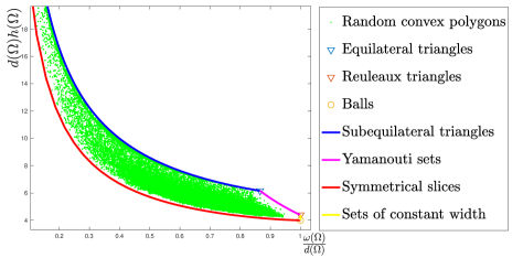
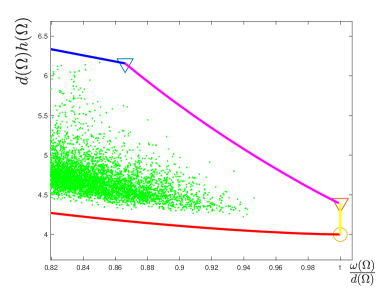
Figure 8. Blaschke–Santaló diagram of the triplet $(\omega,h,d)$.

We are also able to give an explicit, but not sharp, lower bound of the Cheeger constant in terms of the width and the diameter.

Remark 5.2.

Let $\Omega\in\mathcal{K}^{2}$. Then, it holds

(49) $$h(\Omega)>\frac{1}{\omega(\Omega)}+\frac{1}{d(\Omega)}+\sqrt{\left(\frac{1}{\omega(\Omega)}+\frac{1}{d(\Omega)}\right)^{2}-\frac{4-\pi}{\omega(\Omega)d(\Omega)}},$$

where equality is asymptotically achieved by a sequence of thin collapsing rectangles. In order to prove (49), it is enough to consider the inequality

$${\left|\Omega\right|}\leq\omega(\Omega)d(\Omega)$$

and to use the strategy of Lemma 2.9.

5.2. The triplet $(\omega,h,R)$

Proposition 5.3.

Let $\Omega\in\mathcal{K}^{2}$. Then, it holds

(50) $$h(\Omega)\geq\frac{1}{t_{g_{4}^{\Omega}}},$$

where $t_{g_{4}^{\Omega}}$ is the smallest solution of the equation

$$g_{4}^{\Omega}(t):=\frac{(\omega(\Omega)-2t)}{2}\sqrt{4\left(R(\Omega)-t\right)^{2}-\left(\omega(\Omega)-2t\right)^{2}}+2(R(\Omega)-t)^{2}\arcsin{\left(\frac{\omega(\Omega)-2t}{2(R(\Omega)-t)}\right)}=\pi t^{2}$$

on $[0,r(\Omega)]$.

The equality in (50) is achieved by symmetrical spherical slices. Moreover, it holds

(51) $$h(\Omega)\leq h(T_{I}),\qquad\text{ if }\,\omega(\Omega)\leq\frac{3}{2}R(\Omega),$$

where $T_{I}$ is the subequilateral triangle such that $R(T_{I})=R(\Omega)$ and $\omega(T_{I})=\omega(\Omega)$. The equality in (51) is realized by the subequilateral triangle $T_{I}$.

Proof.

Let us start by proving the lower bound (50), by using the strategy given in Lemma 2.9. Let us recall the function defined in (19):

$$\chi:(\omega,R)\longmapsto\frac{\omega}{2}\sqrt{4R^{2}-\omega^{2}}+2R^{2}\arcsin{\frac{\omega}{2R}}.$$

We have, for every $R,\omega>0$,

$$\frac{\partial\chi}{\partial R}(\omega,R)=4R\arcsin{\frac{\omega}{2R}}\geq 0\ \ \ \text{and}\ \ \ \ \frac{\partial\chi}{\partial\omega}(\omega,R)=\sqrt{4R^{2}-\omega^{2}}\geq 0.$$

Thus, using Theorem 2.20, we have, for every $t\in[0,r(\Omega))$,

$$|\Omega_{-t}|\leq\chi(\omega(\Omega_{-t}),R(\Omega_{-t}))\leq\chi(\omega(\Omega)-2t,R(\Omega)-t):=g_{4}^{\Omega}(t),$$

where we use (8) and (9). By Lemma 2.9, we have

$$h(\Omega)\geq\frac{1}{t_{g_{4}^{\Omega}}},$$

where $t_{g_{4}^{\Omega}}$ is the smallest solution to the equation $g_{4}^{\Omega}(t)=\pi t^{2}$ on the interval $[0,r(\Omega)]$. We observe that condition (12) can be easily checked.

Let us now prove the upper bound (51). We recall the inequality (2):

(52) $$h(\Omega)\leq\frac{1}{r(\Omega)}+\sqrt{\frac{\pi}{{\left|\Omega\right|}}},$$

where equality is achieved for instance by circumscribed sets, in particular, by triangles. In order to prove (51), we consider the following facts:

1. In (20), it is proved that, if $\Omega\in\mathcal{K}^{2}$,

   (53) $${\left|\Omega\right|}\geq{\left|T_{I}\right|}\quad\text{if}\,\,\omega(\Omega)\leq\frac{3}{2}R(\Omega),$$

   where $T_{I}$ is the subequilateral triangle with given width and circumradius and nothing is known if $\omega(\Omega)\geq 3/2R(\Omega)$;

2. In Theorem 2.22, see (21), and Theorem 2.23, see (22), it is proved that if

   (54) $$r(\Omega)\geq\begin{cases}r(T_{I})&\text{if}\,\,{\omega(\Omega)\leq\frac{3}{2}R(\Omega)}\\ \omega(\Omega)-R(\Omega)&\text{if}\,\,{\omega(\Omega)\geq\frac{3}{2}R(\Omega)},\end{cases}$$

   where, if $\omega(\Omega)\geq\frac{3}{2}R(\Omega)$, equality is achieved by any set obtained by an equilateral triangle of circumradius $R(\Omega)$ by replacing the edges by three equal circular arcs, in particular each arc of circle is centered on the height relative to the same side.

So, if $\omega(\Omega)\leq\frac{3}{2}R(\Omega)$, combining (52) with (53) and (54), we get the thesis. ∎

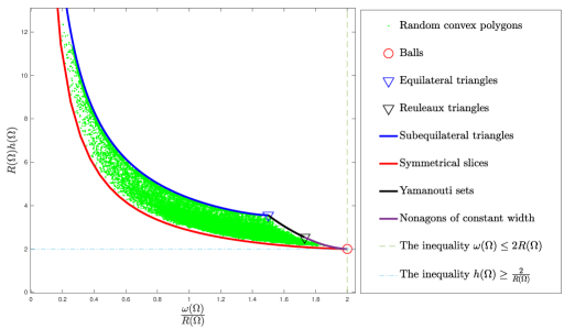
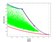
Figure 9. Blaschke–Santaló diagram of the triplet $(\omega,h,R)$.

In the following Remark, we give some not-sharp bounds, that are explicit.

Remark 5.4.

We can prove that

(55) $$h(\Omega)\leq\frac{3}{\omega(\Omega)}+\sqrt{\frac{\pi}{\sqrt{3}R(\Omega)\omega(\Omega)}}.$$

We recall the following inequalities, proved in [39]:

(56) $${\left|\Omega\right|}\geq\sqrt{3}R(\Omega)\omega(\Omega)\ \ \ \text{and}\ \ \ \omega(\Omega)\leq 3r(\Omega).$$

By combining these estimates and the upper bound in (2), we have

$$h(\Omega)\leq\frac{3}{\omega(\Omega)}+\sqrt{\frac{\pi}{\sqrt{3}R(\Omega)\omega(\Omega)}}.$$

Since the equality in (2) is achieved by circumscribed sets, while the equalities in (56) are achieved by equilateral triangles, that are particular circumscribed sets, we have the equality in (55) for equilateral triangles.

Moreover, another not-sharp upper bound can be obtained by using the strategy from Lemma 2.9, starting from

$${\left|\Omega\right|}<2R(\Omega)\omega(\Omega),$$

which is asymptotically achieved by a sequence of rectangles with circumradius that goes to infinity (see [18]). We get ${\left|\Omega_{-t}\right|}\leq 2R(\Omega_{-t})\omega(\Omega_{-t})\leq 2(R(\Omega)-t)(\omega(\Omega)-2t)$ and, consequently,

$$h(\Omega)\geq\frac{4-\pi}{(2R(\Omega)+\omega(\Omega))-\sqrt{(2R(\Omega)+\omega(\Omega))^{2}-(4-\pi)(2R(\Omega)\omega(\Omega))}}.$$

5.3. The triplet $(\omega,h,P)$

Proposition 5.5.

Let $\Omega\in\mathcal{K}^{2}$. Then, it holds

(57) $$h(\Omega)\geq\frac{2}{\omega(\Omega)}+\frac{2\pi}{2P(\Omega)-\pi\omega(\Omega)},$$

where the equality is achieved by stadiums. Moreover, if $P(\Omega)\geq 2\sqrt{3}\omega(\Omega)$, it holds

(58) $$h(\Omega)\leq h(T_{I}),$$

where $T_{I}$ is the subequilateral triangle such that $P(T_{I})=P(\Omega)$ and $\omega(T_{I})=\omega(\Omega)$. The equality in (58) is achieved by the subequilateral triangle $T_{I}$.

Proof.

The inequality (57) is a consequence of (59) and the inequality

$$|\Omega|\leq\frac{\omega(\Omega)}{2}\left(P(\Omega)-\frac{\pi\omega(\Omega)}{2}\right),$$

which is an equality for stadiums (see for example [39] and the references therein).

Let us now assume that $P(\Omega)\geq 2\sqrt{3}\omega(\Omega)$. In order to prove (58), we recall inequality (27):

$$P(\Omega)\leq\sqrt{\frac{4r^{2}(\Omega)\omega^{3}(\Omega)}{(\omega(\Omega)-2r(\Omega))^{2}(4r(\Omega)-\omega(\Omega))}}=:f_{\omega(\Omega)}(r(\Omega))$$

By direct computations, we prove that the continuous function

$$f_{\omega(\Omega)}:r\longmapsto\sqrt{\frac{4r^{2}\omega(\Omega)^{3}}{(\omega(\Omega)-2r)^{2}(4r-\omega(\Omega))}}$$

is strictly increasing on $\left[\frac{\omega(\Omega)}{3},\frac{\omega(\Omega)}{2}\right)$. Let us denote by $g_{\omega(\Omega)}$ the inverse function of $f_{\omega(\Omega)}$, which is also continuous and strictly increasing. We have

$$r(\Omega)\geq g_{\omega(\Omega)}(P(\Omega))=r(T_{I}),$$

where $T_{I}$ is any subequilateral triangle such that $\omega(T_{I})=\omega(\Omega)$ and $P(T_{I})=P(\Omega)$. Moreover, since $P(\Omega)\geq 2\sqrt{3}\omega(\Omega)$, we have by the results contained in [45],

$$|\Omega|\geq|T_{I}|,$$

(see also [39] as a reference). Finally, we obtain

$$h(\Omega)\leq\frac{1}{r(\Omega)}+\sqrt{\frac{\pi}{|\Omega|}}\leq\frac{1}{r(T_{I})}+\sqrt{\frac{\pi}{|T_{I}|}}=h(T_{I}).$$

∎

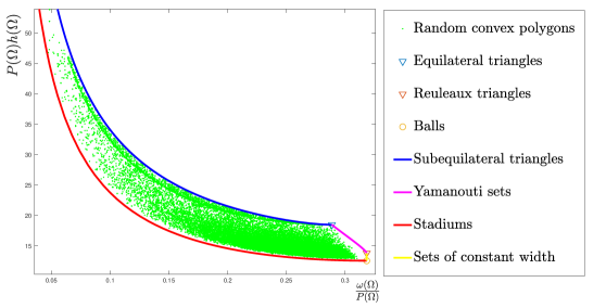
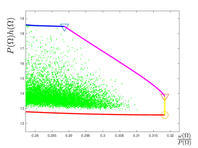
Figure 10. Blaschke–Santaló diagram of the triplet $(\omega,h,P)$.

5.4. The triplet $(\omega,h,|\cdot|)$

Proposition 5.6.

Let $\Omega\in\mathcal{K}^{2}$. Then, it holds

(59) $$h(\Omega)\geq\frac{2}{\omega(\Omega)}+\frac{\pi\omega(\Omega)}{2{\left|\Omega\right|}},$$

where equality is achieved by stadiums. Moreover, it holds

(60) $$h(\Omega)\leq h(T_{I}),$$

where $T_{I}$ is a subequilateral triangle such that $|\Omega|=|T_{I}|$ and $\omega(\Omega)=\omega(T_{I})$. The equality in (60) is achieved by the subequilateral triangle $T_{I}$ (see Figure 11).

Proof.

Let us prove the inequality (59). We recall the lower bound in (2)

$$h(\Omega)\geq\frac{1}{r(\Omega)}+\frac{\pi r(\Omega)}{2|\Omega|},$$

which is an equality if and only if $\Omega$ is a stadium. Since the function $r\longmapsto\frac{1}{r}+\frac{\pi r}{2|\Omega|}$ is strictly decreasing and $r(\Omega)\leq\frac{\omega(\Omega)}{2}$ (where equality holds for stadiums), we obtain (59).

Let us now prove inequality (60). We start by recalling inequality (26):

$$|\Omega|\leq\sqrt{\frac{r^{4}(\Omega)\omega^{3}(\Omega)}{(\omega(\Omega)-2r(\Omega))^{2}(4r(\Omega)-\omega(\Omega))}}=:f_{\omega(\Omega)}(r(\Omega)).$$

By direct computations, we prove that the continuous function

$$f_{\omega(\Omega)}:r\longmapsto\sqrt{\frac{r^{4}\omega(\Omega)^{3}}{(\omega(\Omega)-2r)^{2}(4r-\omega(\Omega))}}$$

is strictly increasing on $\left[\frac{\omega(\Omega)}{3},\frac{\omega(\Omega)}{2}\right)$. Let us denote by $g_{\omega(\Omega)}$ the inverse function of $f_{\omega(\Omega)}$, which is also continuous and strictly increasing. We have

$$r(\Omega)\geq g_{\omega(\Omega)}(|\Omega|)=r(T_{I}),$$

where $T_{I}$ is any subequilateral triangle such that $\omega(T_{I})=\omega(\Omega)$ and $|T_{I}|=|\Omega|$. Thus, we have

$$h(\Omega)\leq\frac{1}{r(\Omega)}+\sqrt{\frac{\pi}{|\Omega|}}\leq\frac{1}{r(T_{I})}+\sqrt{\frac{\pi}{|T_{I}|}}=h(T_{I}),$$

with equality if and only if $\Omega=T_{I}$. ∎

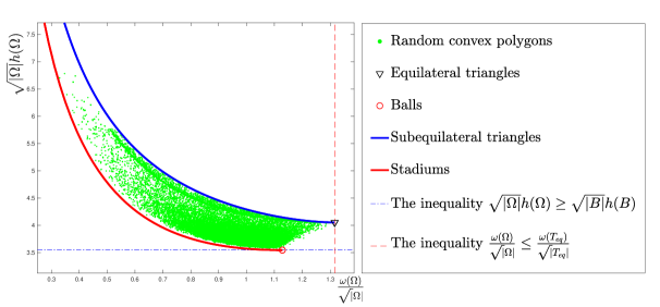
Figure 11. Blaschke–Santaló diagram of the triplet $(\omega,h,|\cdot|)$.

Remark 5.7.

One may use classical convex geometry inequalities to obtain simpler bounds than the implicit one given in (60). Indeed, if we combine the inequalities in (2) and the following classical ones

$$\frac{2}{\omega(\Omega)}\leq\frac{1}{r(\Omega)}\leq\frac{2}{\omega(\Omega)}+\frac{\omega(\Omega)}{\sqrt{3}|\Omega|}$$

where the lower bound is realized in particular by stadiums, and the upper bound by equilateral triangles (see for example [39] and the references therein), we obtain the following inequalities

(61) $$h(\Omega)\leq\frac{2}{\omega(\Omega)}+\frac{\omega(\Omega)}{\sqrt{3}|\Omega|}+\sqrt{\frac{\pi}{|\Omega|}}$$

and

(62) $$h(\Omega)\leq\frac{2}{\omega(\Omega)-\frac{\omega(\Omega)^{3}}{4|\Omega|}}+\sqrt{\frac{\pi}{|\Omega|}}.$$

The bound (61) is achieved by equilateral triangles and (62) is asymptotically achieved by a sequence of thin subequilateral triangles.

5.5. The triplet $(R,h,d)$

Proposition 5.8.

Let $\Omega\in\mathcal{K}^{2}$. Then, it holds

(63) $$h(\Omega)\leq\frac{2R(\Omega)\left(2R(\Omega)+\sqrt{4R(\Omega)^{2}-d(\Omega)^{2}}\right)}{d(\Omega)^{2}\sqrt{4R(\Omega)^{2}-d(\Omega)^{2}}}+\sqrt{\frac{4\pi R(\Omega)^{2}}{d(\Omega)^{3}\sqrt{4R(\Omega)^{2}-d(\Omega)^{2}}}},$$

where the equality is achieved by subequilateral triangles.

Proof.

The inequality (63) is obtained by combining the upper bound in (2), which is an equality for circumscribed sets (in particular subequilateral triangles), and

$$r(\Omega)\geq\frac{d(\Omega)^{2}\sqrt{4R(\Omega)^{2}-d(\Omega)^{2}}}{2R(\Omega)\left(2R(\Omega)+\sqrt{4R(\Omega)^{2}-d(\Omega)^{2}}\right)},\ \ \ \ \ \ |\Omega|\geq\frac{d(\Omega)^{3}\sqrt{4R(\Omega)^{2}-d(\Omega)^{2}}}{4R(\Omega)^{2}},$$

respectively proved in [37] and [22], where the equalities hold only for subequilateral triangles. ∎

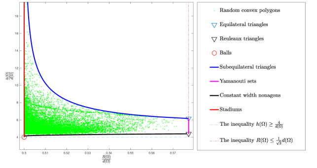
Figure 12. Blaschke–Santaló diagram of the triplet $(R,h,d)$.

5.6. The triplet $(\omega,h,r)$

Proposition 5.9.

Let $\Omega\in\mathcal{K}^{2}$. Then, it holds

(64) $$h(\Omega)\geq\frac{1}{r(\Omega)}+\frac{1}{r(\Omega)}\sqrt{\pi\left(1-\frac{2r(\Omega)}{\omega(\Omega)}\right)\sqrt{\frac{4r(\Omega)}{\omega(\Omega)}-1}},$$

where the equality is achieved by subequilateral triangles (see Figure 13).

Proof.

The proof of (64) is inspired by the proof of [23, Theorem 5]. It is known that the incircle of a set $\Omega$ meets the boundary of $\Omega$ either in two diametrically opposite points, or in three points that form the vertices of a triangle, see [8]. In the first case, we have $\omega(\Omega)=2r(\Omega)$, thus the inequality (64) is equivalent to $h(\Omega)\geq\frac{1}{r(\Omega)}$, which is proved in Proposition 2.10. In the second case, let us denote by $T$ a triangle formed by three lines of support common to $\Omega$ and the incircle. We have $r(\Omega)=r(T)$ and, by $\Omega\subset T$ and the monotonicity with respect to the inclusion, we get

(65) $$h(\Omega)\geq h(T)$$

and

(66) $$\omega(\Omega)\leq\omega(T).$$

So, inequality (64) is equivalent to the following one

$$\frac{1}{r(\Omega)h(\Omega)}f\left(\frac{r(\Omega)}{\omega(\Omega)}\right)\leq 1,$$

where $f:x\in\left[\frac{1}{3},\frac{1}{2}\right]\longmapsto 1+\sqrt{\pi\left(1-2x\right)\sqrt{4x-1}}$. We observe that the function $g:x\in\left[\frac{1}{3},\frac{1}{2}\right]\longmapsto\left(1-2x\right)\sqrt{4x-1}$ is decreasing. Indeed,

$$g^{\prime}(x)=\frac{4(1-3x)}{\sqrt{4x-1}}\leq 0.$$

Thus, $f$ is also decreasing on $\left[\frac{1}{3},\frac{1}{2}\right]$. Then, since $\frac{r(\Omega)}{\omega(\Omega)}\geq\frac{r(T)}{\omega(T)}$ by (66), we have

$$f\left(\frac{r(\Omega)}{\omega(\Omega)}\right)\leq f\left(\frac{r(T)}{\omega(T)}\right).$$

Moreover, we get, by (65),

$$\frac{1}{r(\Omega)h(\Omega)}\leq\frac{1}{r(T)h(T)}.$$

Thus, we obtain

$$\frac{1}{r(\Omega)h(\Omega)}f\left(\frac{r(\Omega)}{\omega(\Omega)}\right)\leq\frac{1}{r(T)h(T)}f\left(\frac{r(T)}{\omega(T)}\right)=\frac{1}{1+r(T)\sqrt{\frac{\pi}{|T|}}}f\left(\frac{r(T)}{\omega(T)}\right),$$

where we used the equality $h(T)=\frac{1}{r(T)}+\sqrt{\frac{\pi}{|T|}}$, which holds because $T$ is a triangle, see [14]. Now, we use the inequality

$$|T|\leq\frac{r(T)^{2}}{\left(1-\frac{2r(T)}{\omega(T)}\right)\sqrt{\frac{4r(T)}{\omega(T)}-1}},$$

which is an equality if and only if $T$ is a subequilateral triangle, see [23, Theorem 5]. So, we have

$$\frac{1}{r(\Omega)h(\Omega)}f\left(\frac{r(\Omega)}{\omega(\Omega)}\right)\leq\frac{1}{1+r(T)\sqrt{\frac{\pi}{|T|}}}f\left(\frac{r(T)}{\omega(T)}\right)\leq 1,$$

which ends the proof. ∎

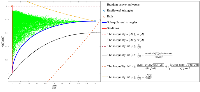
Figure 13. Blaschke–Santaló diagram of the triplet $(\omega,h,r)$.

Remark 5.10.

It is possible to give a not sharp upper bound

$$h(\Omega)\leq\frac{1}{r(\Omega)}+\frac{\sqrt{\pi\sqrt{3}}}{\omega(\Omega)}$$

In order to prove it, we combine the upper bound in (2) and $\omega(\Omega)^{2}\leq\sqrt{3}|\Omega|$, see [39].

6. Conclusions and conjectures

In this last Section, we collect all the conjectures that we can deduce from the numerical approximation of the Blaschke–Santaló diagrams that we have plotted.

Conjecture 1.

As far as the diagram $(\omega,h,d)$ is concerned, we conjecture that, if $\sqrt{3}/2d(\Omega)\leq\omega(\Omega)\leq d(\Omega)$, then for all $\Omega\in\mathcal{K}^{2}$

$$h(\Omega)\leq h(Y)$$

where $Y$ is the Yamanouti set with $\omega(Y)=\omega(\Omega)$ and $d(Y)=d(\Omega)$ (see Figure 8).

Conjecture 2.

As far as the diagram $(\omega,h,R)$ is concerned, we conjecture that, if $\omega(\Omega)\geq\frac{3}{2}R(\Omega)$, then, for all $\Omega\in\mathcal{K}^{2}$,

$$h(\Omega)\leq h(\bar{T}),$$

where $\bar{T}$ is a set obtained by an equilateral triangle of circumradius $R(\Omega)$ by replacing the edges by three equal circular arcs, as described in Theorem 2.23 (see Figure (9)).

Conjecture 3.

As far as the diagram $(\omega,h,P)$ is concerned, we conjecture that, if $\pi\omega(\Omega)\leq P(\Omega)\leq 2\sqrt{3}\omega(\Omega)$, then, for all $\Omega\in\mathcal{K}^{2}$,

$$h(\Omega)\leq h(Y),$$

where $Y$ is the Yamanouti set with $P(Y)=P(\Omega)$ and $\omega(Y)=\omega(\Omega)$. (see Figure (10)).

Conjecture 4.

As far as the diagram $(R,h,d)$ is concerned, we conjecture that

$$h(\Omega)\geq h(N),$$

where $N$ is the set described as follows (see [22]). Let $\Gamma$ and $\gamma$ be the circumcircle and the incircle of a constant width set: they are concentric and $d=\omega=R+r$. The extremal set can be constructed in the following way: an equilateral triangle $PQR$ is inscribed in the circle $\Gamma$, and now we take the circular arcs of radius $R+r$ drawn about the three vertex points. These arcs touch $\gamma$ at the opposite points $\bar{P},\bar{Q},\bar{R}$ of $P,Q,R$, respectively. Furthermore, we construct three circles of radius $(R+r)/2$ that have the sides of the triangle as chords and whose centers lie inside the triangle. The required constant width set has 3-fold symmetry and it is formed by nine arcs of the six constructed circles (see Figure 12).

7. Appendix: Summary tables with the results

In this first table, we summarize the results relative to the diagrams that are completely solved.

Param.	Condition	Inequality	Extremal sets	Ref.
$P,h,A$		$\displaystyle h\leq\frac{P}{A}$	Cheeger to itself	[15]
		$\displaystyle h\geq\frac{P+\sqrt{4\pi A}}{2A}$	circumscribed sets
$r,h,A$		$\displaystyle h\leq\frac{1}{r}+\sqrt{\frac{\pi}{A}}$	circumscribed sets	[14]
		$\displaystyle h\geq\frac{1}{r}+\frac{\pi r}{A}$	stadiums
$P,h,r$		$\displaystyle{h\leq\frac{1}{r}+\sqrt{\frac{2\pi}{Pr}}}$	circumscribed sets	Prop. 4.1
		$\displaystyle{h\geq\frac{1}{r}+\frac{\pi}{P-\pi r}}$	stadiums
$d,h,r$		$\displaystyle{h\leq\frac{1}{r}+\sqrt{\frac{\pi}{r\sqrt{d^{2}-4r^{2}}+r^{2}(\pi-2\arccos{\left(\frac{2r}{d}\right)})}}}$	two-cup bodies	Prop. 4.2
		${h\geq\frac{1}{t_{g_{1}^{\Omega}}}}$ $(i)$	spherical slices/smoothed nonagons
$R,h,r$		$\displaystyle h\leq\frac{1}{r}+\sqrt{\frac{\pi}{2r\left(\sqrt{R^{2}-r^{2}}+r\arcsin\left(\frac{r}{R}\right)\right)}}$	two-cup bodies	Prop. 4.5
		$\displaystyle h\geq\frac{1}{t_{g_{2}^{\Omega}}}$ $(ii)$	spherical slices

$(i)$ $t_{g_{1}^{\Omega}}$ is the smallest solution on $[0,r(\Omega)]$ to

$$g_{1}^{\Omega}(t):=\psi(d(\Omega)-2t,r(\Omega)-t)=\pi t^{2},$$

where

$$\psi(d,r):=\begin{cases}\displaystyle{\frac{3\sqrt{3}r}{2}(\sqrt{d^{2}-3r^{2}}-r)+\frac{3d^{2}}{2}\left(\frac{\pi}{3}-\arccos{\left(\frac{\sqrt{3}r}{d}\right)}\right)},&\text{if}\,\,\,d\leq rD^{*}\vspace{1mm}\\ \displaystyle{r\sqrt{d^{2}-4r^{2}}+\frac{d^{2}}{2}\arcsin{\left(\frac{2r}{d}\right)}},&\text{if}\,\,\,d\geq rD^{*}.\end{cases}$$

and $D^{*}$ is the unique number in $[2,2\sqrt{3}]$ for which the two expression of the function $\psi(d,r)$ are equal.
$(ii)$ $t_{g_{2}^{\Omega}}$ is the smallest solution on $[0,r(\Omega)]$ to

$${g_{2}^{\Omega}}(t):=2\left((r-t)\sqrt{(R(\Omega)-t)^{2}-(r(\Omega)-t)^{2}}+(R(\Omega)-t)^{2}\arcsin{\left(\frac{r(\Omega)-t}{R(\Omega)-t}\right)}\right)=\pi t^{2}.$$

In this second table we summarize the results of the partially solved Blaschke–Santaló diagrams.

Param.	Condition	Inequality	Extremal sets	Ref.
$\omega,h,d$	$\omega\leq\sqrt{3}/2d$	$h\leq\frac{1}{r(\omega,d)}+\sqrt{\frac{2\pi}{\omega d}}$ $(iii)$	subequilateral triangles	Prop. 5.1
	$\sqrt{3}/2d\leq\omega\leq d$	$h\leq\frac{\sqrt{3}}{\sqrt{3}\omega-d}+\sqrt{\frac{2\pi}{\pi\omega^{2}-\sqrt{3}d^{2}+6\omega(\tan\left(\arccos(\frac{\omega}{d})\right)-\arccos(\frac{\omega}{d}))}}$	equilateral triangles
		$h(\Omega)\geq\frac{1}{t_{g_{3}^{\Omega}}}$ $(iv)$	spherical slices
$\omega,h,R$	$\omega\leq 3/2R$	$h\leq\frac{1}{r(\omega,R)}+\sqrt{\frac{\pi}{A(\omega,R)}}$ $(v)$	subequilateral triangles	Prop. 5.3
		$h\geq\frac{1}{t_{g_{4}^{\Omega}}}$ $(vi)$	spherical slices
$\omega,h,P$	$P\geq 2\sqrt{3}\omega$	$h\leq\frac{1}{r(\omega,P)}+\sqrt{\frac{\pi}{A(\omega,P)}}$ $(vii)$	subequilateral triangles	Prop. 5.5
		$h\geq\frac{2}{\omega}+\frac{2\pi}{2P-\pi\omega}$	stadiums
$\omega,h,A$		$h\leq\frac{1}{r(\omega,A)}+\sqrt{\frac{\pi}{A}}$ $(viii)$	subequilateral triangles	Prop. 5.6
		$h\geq\frac{2}{\omega}+\frac{\pi\omega}{2A}$	stadiums
$R,h,d$		$h\leq\frac{2R(2R+\sqrt{4R^{2}-d^{2}})}{d^{2}\sqrt{4R^{2}-d^{2}}}+\sqrt{\frac{4\pi R^{2}}{d^{3}\sqrt{4R^{2}-d^{2}}}}$	subequilateral triangles	Prop. 5.8
$\omega,h,r$		$h\geq\frac{1}{r}+\frac{1}{r}\sqrt{\pi\left(1-\frac{2r}{\omega}\right)\sqrt{\frac{4r}{\omega}-1}}$	subequilateral triangles	Prop. 5.9

$(iii)$ $r(\omega,d)$ is given by

$$d^{2}\left(\omega-2r(\omega,d)\right)^{2}(4r(\omega,d)-\omega)=4r^{4}(\omega,d)\;\omega.$$

$(iv)$ $t_{g_{3}^{\Omega}}$ is the smallest solution to

$${g_{3}^{\Omega}}(t):=f(d(\Omega)-2t,\omega(\Omega)-2t)=\pi t^{2},$$

where

$$f(d,w)=\frac{w}{2}\sqrt{d^{2}-w^{2}}+\frac{d^{2}}{2}\arcsin\left(\frac{w}{d}\right)$$

$(v)$ $r(\omega,R)$ is given by

$$\left(4r(\omega,R)-\omega\right)\left(\omega-2r(\omega,R)\right)=\frac{2r^{3}(\omega,R)}{R}$$

and $A(\omega,R)$ is given by

$$16A(\omega,R)^{6}=R^{2}\omega^{2}\left(16A(\omega,R)^{4}-R^{2}\omega^{6}\right).$$

$(vi)$ $t_{g_{4}^{\Omega}}$ is the smallest solution on $[0,r(\Omega)]$ to

$$g_{4}^{\Omega}(t):=\chi(\omega(\Omega)-2t,R(\Omega)-t)=\pi t^{2},$$

where

$$\chi(\omega,R):=\frac{\omega}{2}\sqrt{4R^{2}-\omega^{2}}+2R^{2}\arcsin{\frac{\omega}{2R}}.$$

$(vii)$ $r(\omega,P)$ is given by

$$(\omega-2r(\omega,P))^{2}(4r(\omega,P)-\omega)P^{2}=4r(\omega,P)^{2}\omega^{3}$$

and $A(\omega,P)$ is the middle root of the equation

$$128PA(\omega,P)^{3}-16\omega(5P^{2}+\omega^{2})A(\omega,P)^{2}+16\omega^{2}P^{3}A(\omega,P)-\omega^{3}P^{4}=0$$

$(viii)$ $r(\omega,A)$ is given by

$$(\omega-2r(\omega,A))^{2}(4r(\omega,A)-\omega)A^{2}=r^{4}(\omega,A)\;\omega^{3}.$$

Finally in this last table we have summarized the not Blaschke–Santaló sharp inequalities that we have found.

Param.	Condition	Inequality	Extremal sets	Ref.
$R,h,A$		$h<\frac{1}{R}+\frac{4R}{A}$	thinning stadiums	[15, 39]
		$h\geq\frac{1}{2R}+\frac{\pi R}{2A}+\sqrt{\frac{\pi}{A}}$	balls
$P,h,R$		$h<\frac{P}{R(P-4R)}$	thinning stadiums	[15, 37]
		$h\geq\frac{4\operatorname{arcsinc}{\left(\frac{4R}{P}\right)}}{P-4R\cos{\left(\operatorname{arcsinc}{\left(\frac{4R}{P}\right)}\right)}}+\sqrt{\frac{8\pi\operatorname{arcsinc}{\left(\frac{4R}{P}\right)}}{P\left(P-4R\cos{\left(\operatorname{arcsinc}{\left(\frac{4R}{P}\right)}\right)}\right)}}$ $(ix)$	balls
$P,h,d$	$2d<P<3d$	$h<\frac{4}{P-2d}+\sqrt{\frac{4\pi}{(P-2d)\sqrt{P(4d-P)}}}$		[14, 15, 39]
	$3d\leq P\leq\pi d$	$h<\frac{4}{P-2d}+\sqrt{\frac{4\pi}{\sqrt{3}d(P-2d)}}$
		$h\geq\frac{4\operatorname{arcsinc}{\left(\frac{2d}{P}\right)}}{P-2d\cos{\left(\operatorname{arcsinc}{\left(\frac{2d}{P}\right)}\right)}}+\sqrt{\frac{8\pi\operatorname{arcsinc}{\left(\frac{2d}{P}\right)}}{(P-2d\cos{\left(\operatorname{arcsinc}{\left(\frac{2d}{P}\right)}\right)}}}$ $(ix)$	balls
$d,h,A$		$h\leq\frac{4}{d}+\frac{2d}{A}$		[14, 15, 39]
		$h<\frac{2d}{A}+\sqrt{\frac{\pi}{A}}$
		$h>\frac{d}{A}+\sqrt{\frac{\pi}{A}}$	thinning two-cup

$(ix)$ where the cardinal-arcsine is defined as

$${\rm sinc}:x\in\mathbb{R}\longmapsto{\rm sinc}(x)=\frac{\sin(x)}{x},\quad{\rm arcsinc}(x)={\rm sinc}^{-1}(x)$$

Acknowledgements: The authors would like to thank Jimmy Lamboley for useful discussions.

I. Ftouhi is supported by the Alexander von Humboldt-Professorship program and by the project ANR-18-CE40- 0013 SHAPO financed by the French Agence Nationale de la Recherche (ANR).

G. Paoli is supported by an Alexander von Humboldt Research Fellowship.

References

• [1] F. Alter and V. Caselles. Uniqueness of the Cheeger set of a convex body. Nonlinear Anal., 70(1):32–44, 2009.
• [2] K. R. Anderson. A reevaluation of an efficient algorithm for determining the convex hull of a finite planar set. Inform. Process. Lett., 7(1):53–55, 1978.
• [3] P. R. S. Antunes and A. Henrot. On the range of the first two Dirichlet and Neumann eigenvalues of the Laplacian. Proc. R. Soc. Lond. Ser. A Math. Phys. Eng. Sci., 467(2130):1577–1603, 2011.
• [4] B. Appleton and H. Talbot. Globally minimal surfaces by continuous maximal flows. IEEE Transactions on Pattern Analysis and Machine Intelligence, 28(1):106–118, 2006.
• [5] W. Blaschke. Eine frage über konvexe Körper. Jahresber. Deutsch. Math. Ver., 25:121–125, 1916.
• [6] B. Bogosel, D. Bucur, and I. Fragalà. Phase field approach to optimal packing problems and related Cheeger clusters. Appl. Math. Optim., 81(1):63–87, 2020.
• [7] T. Bonnesen. Les Problèmes des Isopérimètres et des Isépiphanes. Gauthier-Villaris, 1929.
• [8] T. Bonnesen and W. Fenchel. Theory of convex bodies. BCS Associates, Moscow, ID, 1987. Translated from the German and edited by L. Boron, C. Christenson and B. Smith.
• [9] K. Böröczky, Jr., M. A. Hernández Cifre, and G. Salinas. Optimizing area and perimeter of convex sets for fixed circumradius and inradius. Monatsh. Math., 138(2):95–110, 2003.
• [10] R. Brandenberg and B. González Merino. A complete 3-dimensional Blaschke-Santaló diagram. Math. Inequal. Appl., 20(2):301–348, 2017.
• [11] R. Brandenberg and B. G. Merino. On $(r,d,{R})$-Blaschke-Santaló diagrams with regular $k$-gon gauges. to appear in Revista de la Real Academia de Ciencias Exactas, Físicas y Naturales. Serie A, Matemáticas, 2022.
• [12] A. Delyon, A. Henrot, and Y. Privat. Non-dispersal and density properties of infinite packings. SIAM Journal on Control and Optimization, 57(2):1467–1492, 2019.
• [13] A. Delyon, A. Henrot, and Y. Privat. The missing $({A},d,r)$ diagram. Accepted for publication in Ann. Inst. Fourier, 2020.
• [14] I. Ftouhi. On the Cheeger inequality for convex sets. J. Math. Anal. Appl., 504(2):Paper No. 125443, 26, 2021.
• [15] I. Ftouhi. Complete systems of inequalities relating the perimeter, the area and the Cheeger constant of planar domains. to appear in Comm. in Contemp. Math., 2022.
• [16] I. Ftouhi. Optimal description of Blaschke–Santaló diagrams via numerical shape optimization. https://hal.archives-ouvertes.fr/hal-03646758, 2022. preprint.
• [17] I. Ftouhi and J. Lamboley. Blaschke-Santaló diagram for volume, perimeter, and first Dirichlet eigenvalue. SIAM J. Math. Anal., 53(2):1670–1710, 2021.
• [18] M. Henk and G. A. Tsintsifas. Some inequalities for planar convex figures. Elem. Math., 49(3):120–125, 1994.
• [19] A. Henrot and I. Lucardesi. A Blaschke–Lebesgue theorem for the Cheeger constant. https://arxiv.org/abs/2011.07244, 2020.
• [20] A. Henrot and M. Pierre. Shape variation and optimization, volume 28 of EMS Tracts in Mathematics. European Mathematical Society (EMS), Zürich, 2018.
• [21] M. A. Hernández Cifre. Is there a planar convex set with given width, diameter, and inradius? Amer. Math. Monthly, 107(10):893–900, 2000.
• [22] M. A. Hernández Cifre. Optimizing the perimeter and the area of convex sets with fixed diameter and circumradius. Arch. Math. (Basel), 79(2):147–157, 2002.
• [23] M. A. Hernández Cifre and G. Salinas. Some optimization problems for planar convex figures. Number 70, part I, pages 395–405. 2002. IV International Conference in “Stochastic Geometry, Convex Bodies, Empirical Measures $\&$ Applications to Engineering Science”, Vol. I (Tropea, 2001).
• [24] M. A. Hernández Cifre, G. Salinas, and S. Gomis. Complete systems of inequalities. Journal of inequalities in pure and applied mathematics, 2(1), March 2001.
• [25] M. A. Hernández Cifre and S. Segura Gomis. The missing boundaries of the Santaló diagrams for the cases $(d,\omega,R)$ and $(\omega,R,r)$. Discrete Comput. Geom., 23(3):381–388, 2000.
• [26] T. Jahn. Extremal radii, diameter and minimum width in generalized Minkowski spaces. Rocky Mountain J. Math., 47(3):825–848, 2017.
• [27] J.Cheeger. A lower bound for the smallest eigenvalue of the Laplacian. A Symposium in Honor of Salomon Bochner, page 195–199, 1970.
• [28] B. Kawohl and T. Lachand-Robert. Characterization of Cheeger sets for convex subsets of the plane. Pacific J. Math., 225(1):103–118, 2006.
• [29] J. B. Keller. Plate failure under pressure. SIAM Review, 22(11):227–228, 1980.
• [30] T. Kubota. Einige ungleischheitsbezichungen über eilinien und eiflächen. Sci. Rep. of the Tohoku Univ. Ser. (1), 12:45–65, 1923.
• [31] S. Larson. Corrigendum to “A bound for the perimeter of inner parallel bodies” [J. Funct. Anal. 271 (3) (2016) 610–619]. J. Funct. Anal., 279(5):108574, 2, 2020.
• [32] I. Lucardesi and D. Zucco. On Blaschke-Santaló diagrams for the torsional rigidity and the first Dirichlet eigenvalue. Ann. Mat. Pura Appl. (4), 201(1):175–201, 2022.
• [33] E. Parini. An introduction to the Cheeger problem. Surv. Math. Appl., 6:9–21, 2011.
• [34] E. Parini. Reverse Cheeger inequality for planar convex sets. J. Convex Anal., 24(1):107–122, 2017.
• [35] F. P. Preparata and M. I. Shamos. Computational geometry. Texts and Monographs in Computer Science. Springer-Verlag, New York, 1985. An introduction.
• [36] V. Sander. http://cglab.ca/ sander/misc/ConvexGeneration/convex.html.
• [37] L. Santaló. Sobre los sistemas completos de desigualdades entre treselementos de una figura convexa plana. Math. Notae, 17:82–104, 1961.
• [38] R. Schneider. Convex Bodies: The Brunn-Minkowski Theory. Cambridge University Press, 2nd expanded edition edition, 2013.
• [39] P. R. Scott and P. W. Awyong. Inequalities for convex sets. JIPAM. J. Inequal. Pure Appl. Math., 1(1):Article 6, 6, 2000.
• [40] M. Sholander. On certain minimum problems in the theory of convex curves. Trans. Amer. Math. Soc., 73:139–173, 1952.
• [41] G. Strang. Maximal flow through a domain. Math. Programming, 26(2):123–143, 1983.
• [42] B. Sz.-Nagy. Über Parallelmengen nichtkonvexer ebener Bereiche. Acta Sci. Math. (Szeged), 20:36–47, 1959.
• [43] P. Valtr. Probability that $n$ random points are in convex position. Discrete Comput. Geom., 13(3-4):637–643, 1995.
• [44] M. Van den Berg, G. Buttazzo, and A. Pratelli. On the relations between principal eigenvalue and torsional rigidity. Commun. Contemp. Math. (to appear), 2020.
• [45] M. Yamanouti. Notes on closed convex figures. Proc. Phys.-Math. Soc. Japan, III. Ser., 14:605–609, 1932.