Normalized/Clipped SGD with Perturbation for Differentially Private Non-Convex Optimization

Abstract

By ensuring differential privacy in the learning algorithms, one can rigorously mitigate the risk of large models memorizing sensitive training data. In this paper, we study two algorithms for this purpose, i.e., DP-SGD and DP-NSGD, which first clip or normalize per-sample gradients to bound the sensitivity and then add noise to obfuscate the exact information. We analyze the convergence behavior of these two algorithms in the non-convex optimization setting with two common assumptions and achieve a rate $\mathcal{O}\left(\sqrt[4]{\frac{d\log(1/\delta)}{N^{2}\epsilon^{2}}}\right)$ of the gradient norm for a $d$-dimensional model, $N$ samples and $(\epsilon,\delta)$-DP, which improves over previous bounds under much weaker assumptions. Specifically, we introduce a regularizing factor in DP-NSGD and show that it is crucial in the convergence proof and subtly controls the bias and noise trade-off. Our proof deliberately handles the per-sample gradient clipping and normalization that are specified for the private setting. Empirically, we demonstrate that these two algorithms achieve similar best accuracy while DP-NSGD is comparatively easier to tune than DP-SGD and hence may help further save the privacy budget when accounting the tuning effort.

1 Introduction

Modern applications of machine learning strongly rely on training models with sensitive datasets, including medical records, real-life locations, browsing histories and so on. These successful applications raise an unavoidable risk of privacy leakage, especially when large models are shown to be able to memorize training data [10]. Differential Privacy (DP) is a powerful and flexible framework [18] to quantify the influence of each individual and reduce the privacy risk. Specifically, we study the machine learning problem in the formalism of minimizing empirical risk privately:

$$\min_{{\bm{x}}\in\mathbb{R}^{d}}f({\bm{x}})\triangleq\mathbb{E}_{\xi}[\ell({\bm{x}},\xi)]=\frac{1}{N}\sum_{i=1}^{N}\ell({\bm{x}},\xi_{i}),$$ (1)

where the objective $f({\bm{x}})$ is an average of losses evaluated at each data point.

In order to provably achieve the privacy guarantee, one popular algorithm is differentially private stochastic gradient descent or DP-SGD for abbreviation, which clips per-sample gradients with a preset threshold and perturbs the gradients with Gaussian noise at each iteration. Formally, given a set of gradients $\{{\bm{g}}^{(i)},i\in\mathcal{S}\subset[N]\}$ computed at some data points and a threshold $c>0$, a learning rate $\eta>0$ and a noise multiplier $\sigma$, the updating rule goes from ${\bm{x}}$ to the following

$${\bm{x}}^{+}={\bm{x}}-\eta\left(\frac{1}{|\mathcal{S}|}\sum_{i\in\mathcal{S}}\bar{h}^{(i)}{\bm{g}}^{(i)}+\bar{{\bm{z}}}\right),$$ (2)

where $\bar{{\bm{z}}}\sim\mathcal{N}(0,c^{2}\sigma^{2}{\bm{I}}_{d})$ is an isotropic Gaussian noise and $\bar{h}^{(i)}=\min\{1,c/\|{\bm{g}}^{(i)}\|\}$ is the per-sample clipping factor. Intuitively speaking, the per-sample clipping procedure controls the influence of one individual. DP-SGD [1] has made a benchmark impact in deep learning with differential privacy, which is also referred to as gradient perturbation approach. It has been extensively studied from many aspects, e.g., convergence [5, 46], privacy analysis [1], adaptive clipping threshold [4, 2, 36], hyperparameter choices [28, 33, 34, 32] and so forth [6, 7, 35].

Another natural option to achieve differential privacy is normalized gradient with perturbation, which we coin “DP-NSGD”. It normalizes per-sample gradients to control individual contribution and then adds noise accordingly. The update formula is the same as (2) except replacing $\bar{h}^{(i)}$ with a per-sample normalization factor

$$h^{(i)}=\frac{1}{r+\|{\bm{g}}^{(i)}\|},$$ (3)

and replacing $\bar{{\bm{z}}}$ with ${\bm{z}}\in\mathcal{N}(0,\sigma^{2}\mathbf{I}_{d})$ since each sample’s influence is normalized to be $1$. In (3), we introduce a regularizer $r>0$, which not only addresses the issue of ill-conditioned division but also controls the bias and noise trade-off as we will see in the analysis.

An intuitive thought that one may favor DP-NSGD is that the clipping is hard to tune due to the changing statistics of the gradients over the training trajectory [2, 36]. In more details, the injected Gaussian noise $\eta\bar{{\bm{z}}}$ in (2) is proportional to the clipping threshold $c$ and this noise component would dominate over the gradient component $\sum\bar{h}^{(i)}{\bm{g}}^{(i)}/|\mathcal{S}|$, when the gradients $\|{\bm{g}}^{(i)}\|\ll c$ are getting small as optimization algorithm iterates, thus hindering the overall convergence. DP-NSGD aims to alleviate this problem by replacing $\bar{h}^{(i)}$ in (2) with a per-sample gradient normalization factor $h^{(i)}$ in (3), thus enhancing the signal component $g^{(i)}$ when it is too small.

It is obvious that both clipping and normalization introduce bias that might prevent the optimizers from converging [12, 50]. Most of previous works on the convergence of DP-SGD [5, 4, 46] neglect the effect of such biases by assuming a global gradient upper bound of the problem, which does not exist for the cases of deep neural network models. Chen et al.[12] have made a first attempt to understand gradient clipping, but their results strongly rely on a symmetric assumption which is not that realistic.

In this paper, we consider both the effect of per-sample normalization/clipping and the injected Gaussian perturbation in the convergence analysis. If properly setting the hyper-parameters, we achieve $\mathcal{O}\left(\sqrt[4]{\frac{d\log(1/\delta)}{N^{2}\epsilon^{2}}}\right)$ convergence rate of the gradient norm for the general non-convex objectives with $d$-dimensional model, $N$ samples and $(\epsilon,\delta)$-DP, under only two weak assumptions [48], $(L_{0},L_{1})$-generalized smoothness and $(\tau_{0},\tau_{1})$-bounded gradient variance. These assumptions are very mild compared to the usual ones as they allow the smoothness coefficient and the gradient variance growing with the norm of gradient, which is widely observed in the setting of deep learning.

Our contributions are summarized as follows.

• For the differentially private empirical risk minimization, we establish the convergence rate of the DP-NSGD and the DP-SGD algorithms for general non-convex objectives with only an $(L_{0},L_{1})$-smoothness condition, and explicitly characterizes the bias of the per-sample clipping or normalization.

• For the DP-NSGD algorithm, we introduce a regularizing factor which turns out to be crucial in the convergence analysis and induces interesting trade-off between the bias due to normalization and the decaying rate of our upper bound.

• We identify one key difference in the proofs of the DP-NSGD and DP-SGD. As the gradient norm approaches zero, DP-NSGD cannot guarantee the function value to drop along the expected descent direction, and introduce an non-vanishing term that depends on the regularizer and the gradient variance.

• We evaluate their empirical performance on deep models with $(\epsilon,\delta)$-DP and show that both DP-NSGD and DP-SGD can achieve comparable accuracy but the former is easier to tune than the later.

After introducing our problem setup in Section 2, we present the algorithms and theorems in Section 3 and show numerical experiments on vision tasks in Section 4. We make concluding remarks in Section 5.

Table 1: Expected gradient norm bounds (the smaller, the better) for non-convex empirical risk minimization with/without $(\epsilon,\delta)$-DP guarantee. All the algorithms assume certain bound on the gradient noise, which may be different from one another. Notations: $N,T$ and $d$ are the number of samples, the number of iterations and the number of parameters, respectively. All bounds should be read as $\mathcal{O}(\cdot)$ and $\log\frac{1}{\delta}$ is omitted.

Algorithm	Condition	Bias handled	Bound
SGD [21]	$L$-Smooth & $V$-Bounded Variance	N/A	${\mathcal{O}}\left(\frac{1}{\sqrt{T}}+\frac{\sqrt{V}}{\sqrt[4]{T}}\right)$
Clipped SGD [48]	$(L_{0},L_{1})$-Smooth & $V$-Bounded Variance	$\surd$	${\mathcal{O}}\left(\frac{V^{2}}{\sqrt{T}}+\frac{V^{3/2}}{\sqrt[4]{T}}\right)$
DP-NSGD* [15]	$L$-Smooth & quasar-Convex	$\surd$	$\mathcal{O}\left(\frac{D_{X}\sqrt{d}}{N\epsilon}+\mathbb{E}_{i}\|{\bm{x}}_{i}^{*}-{\bm{x}}^{*}\|\right)$ **
DP-GD [40]	L-Smooth & Bounded Gradient	$\times$	$\tilde{{\mathcal{O}}}\left(\frac{d}{\log N\epsilon^{2}}\right)$
DP-(N)SGD (Ours)	$(L_{0},L_{1})$-Generalized Smooth	$\surd$	${\mathcal{O}}\left(\sqrt[4]{\frac{d}{N^{2}\epsilon^{2}}}\right)$

• To be precise, [15] studies a client-level DP optimizer in a federated setting. Their optimizer, DP-NormFedAvg, uses vanilla GD for each client and normalizes the contribution of every client. Sharing similar motivations with our centralized DP-NSGD, their contributions are roughly credited to DP-NSGD.

• Here $\|{\bm{x}}_{i}^{\ast}-{\bm{x}}^{\ast}\|$ measures heterogeneity via the distance between the $i$-th client’s local minimizer ${\bm{x}}_{i}^{\ast}$ to the global minimizer ${\bm{x}}^{\ast}$, and $D_{X}\triangleq\|{\bm{x}}_{0}-{\bm{x}}^{\ast}\|$.

2 Problem Setup

2.1 Notations

Denote the private dataset as $\mathbb{D}=\{\xi_{i},1\leq i\leq N\}$. The loss $\ell({\bm{x}},\xi)$ is defined for every model parameters ${\bm{x}}\in\mathbb{R}^{d}$ and sample instance $\xi$. In the seuqel, $\|{\bm{x}}\|$ is denoted as the $\ell_{2}$ norm of a vector ${\bm{x}}\in\mathbb{R}^{d}$, without other specifications. Our target is to minimize the empirical average loss (1) satisfying $(\epsilon,\delta)$-differential privacy [17]. From time to time, we also use $\nabla\ell({\bm{x}},\xi)$ to denote the gradient of $\ell(\cdot,\cdot)$ w.r.t. ${\bm{x}}$ evaluated at $({\bm{x}},\xi)$. We are given an oracle to have multiple stochastic unbiased estimates ${\bm{g}}^{(i)}$ for the gradient $\nabla f({\bm{x}})$ of objective at any point.

Definition 2.1 ($(\epsilon,\delta)$-DP).

A randomized mechanism $\mathcal{M}$ guarantees $(\epsilon,\delta)$-differentially privacy if for any two neighboring input datasets $\mathbb{D}\sim\mathbb{D}^{\prime}$ ($\mathbb{D}^{\prime}$ differ from $\mathbb{D}$ by substituting one record of data) and for any subset of output $S$ it holds that $\text{Pr}[\mathcal{M}(\mathbb{D})\in S]\leq e^{\epsilon}\text{Pr}[\mathcal{M}(\mathbb{D}^{\prime})\in S]+\delta$.

Besides, we also define the following notations to illustrate the bound we derived. We write $f(\cdot)=\mathcal{O}(g(\cdot))$, $f(\cdot)=\Omega(g(\cdot))$ to denote $f(\cdot)/g(\cdot)$ is upper or lower bounded by a positive constant. We also write $f(\cdot)=\Theta(g(\cdot))$ to denote that $f(\cdot)=\Omega(g(\cdot))$ and $f(\cdot)=\Omega(g(\cdot))$. Throughout this paper, we use $\mathbb{E}$ to represent taking expectation over the randomness of optimization procedures, including drawing gradients estimates ${\bm{g}}$ and adding extra Gaussian perturbation ${\bm{z}}$, while $\mathbb{E}_{k}$ takes conditional expectation given ${\bm{x}}_{k}$.

In this non-convex setting, we measure the utility of some algorithm via bounding the expected minimum gradient norm $\mathbb{E}\left[\min_{0\leq k<T}\|\nabla f({\bm{x}}_{k})\|\right]$. If we want to measure the utility via bounding function values, the extra convex condition or its weakened versions are essential.

2.2 Assumptions on Smoothness and Variance

Definition 2.2.

We say that a continuously differentiable function $f({\bm{x}})$ is $(L_{0},L_{1})$-generalized smooth, if for all ${\bm{x}},{\bm{y}}\in\mathbb{R}^{d}$, we have $\|\nabla f({\bm{x}})-\nabla f({\bm{y}})\|\leq(L_{0}+L_{1}\|\nabla f({\bm{x}})\|)\|{\bm{x}}-{\bm{y}}\|$.

Firstly appearing in [48], a similar condition is derived via empirical observations that the smoothness $\|\nabla^{2}f({\bm{x}})\|$ increases with the gradient norm $\|\nabla f({\bm{x}})\|$ in training language models. If we set $L_{1}=0$, then Definition 2.2 turns into the usually assumed $L$-smooth. This relaxed notion of smoothness, Definition 2.2, and lower bounded function value together constitute our first assumption below.

Assumption 2.1.

We assume that $f({\bm{x}})$ is $(L_{0},L_{1})$-generalized smooth, Definition 2.2. We also assume $D_{f}\triangleq f({\bm{x}}_{0})-f^{\ast}<\infty$ where $f^{\ast}=\inf_{{\bm{x}}\in\mathbb{R}}f({\bm{x}})$ is the global minimum of $f(\cdot)$.

We do not assume an upper bound on $D_{X}\triangleq\|{\bm{x}}_{0}-{\bm{x}}^{*}\|$, which may scale with the model dimension.

Moreover, to handle the stochasticity in gradient estimates, we employ the following almost sure upper bound on the gradient variance as another assumption.

Assumption 2.2.

For all ${\bm{x}}\in\mathbb{R}^{d}$, $\mathbb{E}[{\bm{g}}]=\nabla f({\bm{x}})$. Furthermore, there exists $\tau_{0}>0$ and $0\leq\tau_{1}<1$, such that with probability $1$, it holds $\|{\bm{g}}-\nabla f({\bm{x}})\|\leq\tau_{0}+\tau_{1}\|\nabla f({\bm{x}})\|$.

Previously, [48] and [47] obtained their results under the exact assumption of $\tau_{1}=0$. In comparison, Assumption 2.2 is much weaker, as it allows the deviation $\|{\bm{g}}-\nabla f({\bm{x}})\|$ grows with respect to the gradient norm $\|\nabla f({\bm{x}})\|$, matching practical observation.

The almost surely error bound sharply controls $h=1/(r+\|{\bm{g}}\|)$ with probability $1$ by

$$\frac{1}{r+\tau_{0}+(1+\tau_{1})\|\nabla f({\bm{x}})\|}\leq h\leq\frac{1}{r-\tau_{0}+(1-\tau_{1})\|\nabla f({\bm{x}})\|}.$$

Analysis in [25] can work with an expectation version of Assumption 2.2: $\mathbb{E}\left[\|{\bm{g}}-\nabla f({\bm{x}})\|^{2}\right]\leq\tau_{0}+\tau_{1}\|\nabla f({\bm{x}})\|^{2}$ because they are allowed to control the error $\|{\bm{g}}-\nabla f({\bm{x}})\|$ via momentum in the non-private context.

In the non-private case, one usually chooses a mini-batch of data ${\bm{g}}=\dfrac{1}{|\mathcal{S}|}\sum_{i\in\mathcal{S}}\nabla f({\bm{x}},\xi_{i})$. Thereafter, one can reduce the variance factors $(\tau_{0},\tau_{1})$ with large batch size $|\mathcal{S}_{k}|$. However, in our private setting, clipping or normalization should apply on per-sample gradients, indicating that we cannot effectively reduce the variance via large batch size.

2.3 More Related Works

Private Deep Learning:

Many papers [11, 41, 40, 27, 46, 42, 4] have made attempts to theoretically analyze gradient perturbation approaches in various settings, including (strongly) convex or non-convex objectives. However, these papers did not take gradient clipping into consideration, and simply treat DP-SGD as SGD with extra Gaussian noise. Chen et al.[12] made a first attempt to understand gradient clipping, but their results strongly rely on a symmetric assumption which is considered as unrealistic. Very recently, Zhang et al.[49] studied the convergence of DP-FedAvg with clipping, the federated averaging algorithm with differential privacy guarantee.

As for algorithms involving normalizing, Das et al.[15] studied DP-FedAvg with normalizing, which normalizes each client’s update to unit-norm vector and then conducts the usual Fed-Avg operation. Their convergence analysis is based on one-point/quasar convexity and $L$-smoothness.

All these mentioned results are hard to compare due to the differences of the settings, assumptions and algorithms. We only present a part of them in Table 1.

Non-Convex Stochastic Optimization: Ghadimi and Lan[21] established the convergence of randomized SGD for non-convex optimization. The objective is assumed to be $L$-smooth and the randomness on gradients is assumed to be light-tailed with factor $V$. We note that the rate ${\mathcal{O}}(V/\sqrt[4]{T})$ has been shown to be optimal in the worst-case under the same condition [3].

Outside the privacy community, understanding gradient normalization and clipping is also crucial in analyzing adaptive stochastic optimization methods, including AdaGrad [16], RMSProp [24], Adam [26] and normalized SGD [13]. However, with the average of a mini-batch of gradient estimates being clipped, this batch gradient clipping differs greatly from the per-sample gradient clipping in the private context. Zhang et al.[48] and Zhang et al.[47] showed the superiority of batch gradient clipping with and without momentum respectively under $(L_{0},L_{1})$-smoothness condition for non-convex optimization. Due to a strong connection between clipping and normalization, we also assume this relaxed condition in our analysis. We further explore this condition for some specific cases in great details. Cutkosky and Mehta[14] found that a fine integration of clipping, normalization and momentum, can overcome heavy-tailed gradient variances via a high-probability bound. Jin et al.[25] discovered that normalized SGD with momentum is also distributionally robust.

3 Normalized/Clipped Stochastic Gradient Descent with Perturbation

3.1 Algorithms and Their Privacy Guarantees

Algorithm 1 Differentially Private Normalized Stochastic Gradient Descent, DP-NSGD

  Input: initial point ${\bm{x}}_{0}$; number of epochs $T$; default learning rates $\eta_{k}$; mini batch size $B$; noise multiplier $\sigma$; regularizer $r$.

  for $k=0$ to $T-1$ do

     Draw a mini-batch $\mathcal{S}_{k}$ of size $B$ and compute individual gradients ${\bm{g}}_{k}^{i}$ at point ${\bm{x}}_{k}$ where $i\in\mathcal{S}_{k}$.

     For $i\in\mathcal{S}_{k}$, compute per-sample normalizing factor

$$h_{k}^{(i)}=\frac{1}{r+\|{\bm{g}}_{k}^{(i)}\|}.$$

     Draw ${\bm{z}}_{k}\sim\mathcal{N}(0,\sigma^{2}{\bm{I}}_{d})$ and update the parameters by

$${\bm{x}}_{k+1}={\bm{x}}_{k}-\eta_{k}\left(\frac{1}{B}\sum_{i\in\mathcal{S}_{k}}h_{k}^{(i)}{\bm{g}}_{k}^{(i)}+{\bm{z}}_{k}\right).$$

  end for

Since no literature formally displays DP-NSGD in a centralized setting, we present it in Algorithm 1. Compared to the usual SGD update, DP-NSGD contains two more steps: per-sample gradient normalization, i.e., multiplying ${\bm{g}}_{k}^{(i)}$ with $h_{k}^{(i)}$, and noise injection, i.e., adding ${\bm{z}}_{k}$. The normalization well controls each sample’s contribution to the update and the noise obfuscates the exact information.

The well-known DP-SGD [1] replaces the normalization with clipping, i.e., replacing $h_{k}^{(i)}$ with $\bar{h}_{k}^{(i)}=\min\left\{1,c/\|{\bm{g}}_{k}\|\right\}$ and replacing $z_{k}$ with $\bar{z}_{k}\sim\mathcal{N}(0,c\sigma^{2}{\bm{I}}_{d})$ in Algorithm 1. DP-SGD introduces a new hyper-parameter, the clipping threshold $c$.

To facilitate the common practice in private deep learning, we adopt uniform sub-sampling without sampling for both theory and experiments, instead of Poisson sub-sampling originally adopted in DP-SGD [1]. Due to this difference, the following lemma shares the same expression as Theorem 1 in [1], but requires a new proof. Deferred in Appendix E, this simple proof combines amplified privacy accountant by sub-sampling in [8] with the tight composition theorem for Renyi DP, [31].

Lemma 3.1 (Privacy Guarantee).

Provided that $B<0.1N$, there exists absolute constants $c_{1},c_{2}>0$ so that DP-SGD and DP-NSGD are $(\epsilon,\delta)$-differentially private for any $\epsilon<c_{1}B^{2}T/N^{2}$ and $\delta>0$ if we choose $\sigma\geq c_{2}\frac{B\sqrt{T\log(1/\delta)}}{N\epsilon}$.

3.2 Convergence Guarantee of DP-NSGD

Theorem 3.2.

Suppose that the objective $f({\bm{x}})$ satisfies Assumption 2.1 and 2.2. Given any noise multiplier $\sigma$ and a regularizer $r>\tau_{0}$, we run DP-NSGD (Algorithm 1) using constant learning rate

$$\eta=\sqrt{\frac{2}{(L_{1}(r+\tau_{0})+L_{0})Td\sigma^{2}}},$$ (4)

with sufficiently many iterations $T$ (larger than some constant determined by $(\sigma^{2},d,L,\tau,r)$, as specified in Lemma B.2). We can obtain the following upper bound on gradient norm

$$\mathbb{E}\left[\min_{0\leq k<T}\|\nabla f({\bm{x}}_{k})\|\right]\leq C\left(\sqrt[4]{\frac{(D_{f}+1)^{2}r^{3}d\sigma^{2}}{T}}+\sqrt[4]{\frac{1}{Tr^{3}d\sigma^{2}}}\right)+\frac{8(r+2\tau_{0})\tau_{0}^{2}}{r(r+\tau_{0})(1-\tau_{1})^{3}},$$ (5)

where $C$ is a constant depending on $(\tau_{0},\tau_{1})$ and $(L_{0},L_{1})$.

Theorem 3.2 is a general convergence for normalized SGD with perturbation. To achieve $(\epsilon,\delta)$-differential privacy, we can choose specific noise multiplier $\sigma$ and running iterations $T$.

Corollary 3.3.

Under the same conditions of Theorem 3.2, we use $\sigma=c_{2}B\sqrt{T\log\frac{1}{\delta}}/(N\epsilon)$ with $c_{2}$ from Lemma 3.1 and set $T\geq{\mathcal{O}}(N^{2}\epsilon^{2}/(B^{2}r^{3}d\log\frac{1}{\delta}))$. If we have sufficiently many samples (larger than $L_{1}$ times some constant determined by $(\epsilon,\delta,d,L,\tau,r,B)$, as specified in Lemma B.3), there holds the following privacy-utility trade-off

$$\mathbb{E}\left[\min_{0\leq k<T}\|\nabla f({\bm{x}}_{k})\|\right]\leq C^{\prime}\sqrt[4]{\frac{dr^{3}\log(1/\delta)}{N^{2}\epsilon^{2}}}+\frac{8(r+2\tau_{0})\tau_{0}^{2}}{r(r+\tau_{0})(1-\tau_{1})^{3}},$$ (6)

where $C^{\prime}$ is a constant depending on $(\tau_{0},\tau_{1})$, $(L_{0},L_{1})$, $D_{f}$ and $B$.

There are two major obstacles in proving this theorem. One is to handle the normalized gradients, which is solved by carefully using $r$ and dividing the range of $\|\nabla f({\bm{x}}_{k})\|$ into two cases. The other is to handle the Gaussian perturbation ${\bm{z}}$, whose variance $\sigma^{2}$ could even grow linearly with $T$. This is solved by setting the learning rate $\eta$ proportionally to $1/\sigma$ in (4). Combining the two steps together, we reach the privacy-utility trade-off in Corollary 3.3.

Proof Sketch of Theorem 3.2.

We firstly establish a descent inequality as in Lemma A.2 via exploiting the $(L_{0},L_{1})$-generalized smooth condition in Assumption 2.1,

$$\mathbb{E}_{k}\left[f({\bm{x}}_{k+1})\right]-f({\bm{x}}_{k})\leq-\underbrace{\eta\mathbb{E}_{k}\left[\langle h_{k}\nabla f({\bm{x}}_{k}),{\bm{g}}_{k}\rangle\right]}_{\mathfrak{A}}+\underbrace{\frac{L_{0}+L_{1}\|\nabla f({\bm{x}}_{k})\|}{2}\eta^{2}\left(d\sigma^{2}+\mathbb{E}_{k}\left\|h_{k}{\bm{g}}_{k}\right\|^{2}\right)}_{\mathfrak{B}}.$$

In the above expression, we use $\mathbb{E}_{k}$ to denote taking expectation of $\{{\bm{g}}_{k}^{(i)},i\in\mathcal{S}_{k}\}$ and ${\bm{z}}_{k}$ conditioned on the past, especially ${\bm{x}}_{k}$. Next, in Lemma B.1, we upper bound the second order term $\mathfrak{B}$ by a constant $\mathcal{O}(\eta^{2})$ plus a term like $\eta\mathbb{E}_{k}\left[h_{k}\|\nabla f({\bm{x}}_{k})\|^{2}\right]$, which is compatible to $\mathfrak{A}$. In order to find simplified lower bound for $\mathfrak{A}$, we separate the time index $\{0,1,\cdots,T-1\}$ into two cases $\mathcal{U}:=\left\{0\leq k<T:\|\nabla f({\bm{x}}_{k})\|\geq\frac{\tau_{0}}{1-\tau_{1}}\right\}$ and $\mathcal{U}^{c}$. Specifically, in Lemma A.3, we find that for $k\in\mathcal{U}$, the first order term $\mathfrak{A}$ is $\Omega(\eta\|\nabla f({\bm{x}}_{k})\|)$ (see (17) in Appendix A); for $k\notin\mathcal{U}$, the first order term $\mathfrak{A}$ is $\Omega(\eta(\|\nabla f({\bm{x}}_{k})\|^{2}/r-\tau_{0}^{3}/r^{2}))$ (see (18) in Appendix A). Then our result follows from summing up descent inequalities and scaling $\eta$ deliberately. ∎

There are rich literature investigating the convergence properties of normalized gradient methods in the non-private non-convex optimization setting. These results heavily rely on the following inequality to control the amount of descent

$$-\left\langle\nabla f({\bm{x}}_{k}),\frac{{\bm{g}}_{k}}{\|{\bm{g}}_{k}\|}\right\rangle\leq-\|\nabla f({\bm{x}}_{k})\|+2\|{\bm{g}}_{k}-\nabla f({\bm{x}}_{k})\|.$$ (7)

Pitifully, based on this inequality, one unavoidably needs to control the error term $\|{\bm{g}}_{k}-\nabla f({\bm{x}}_{k})\|$ well to have the overall convergence. In practice, You et al.[45] used large batch size $B\sim\mathcal{O}(T)$ to reduce the variance. However, this trick cannot apply in the private setting due to per-sample gradient processing, e.g., clipping or normalization. In theory, Cutkosky and Mehta [13] and Jin et al.[25] use momentum techniques with a properly scaled weight decay and obtain a convergence rate $\mathbb{E}\|\nabla f({\bm{x}}_{T})\|=\mathcal{O}(1/\sqrt[4]{T})$, which is comparable with the usual SGD in the non-convex setup [21]. However, momentum techniques do not apply well in the private setting either, because we only have access to previous descent directions with noise due to the composite differential privacy requirement. As far as we know, there is no successful application of momentum in the private community, either practically or theoretically.

In this paper, we view the regularizer $r$ as a tunable hyperparameter, and make our upper bound decay as fast as possible $\mathcal{O}(1/\sqrt[4]{T})$ by tuning $r$. However, due to the restrictions imposed by privacy protection, we are unable to properly employ large batch size or use momentum, thus leaving a strictly positive bound $\mathcal{O}(\tau_{0}^{2}/r)$ in the right hand side of Theorem 3.2 and Corollary 3.3. Another observation is that $r$ trades off between the non-vanishing bound $\mathcal{O}(\tau_{0}^{2}/r)$ and the decaying term of $\mathcal{O}\left(\sqrt[4]{dr^{3}\log\frac{1}{\delta}/(N^{2}\epsilon^{2})}\right)$.

3.3 Convergence Guarantee of DP-SGD

We now turn our attention to clipped DP-SGD. Before we compare the distinctions, we present the following theorem on convergence.

Theorem 3.4.

Suppose that the objective $f({\bm{x}})$ satisfies Assumption 2.1 and 2.2. Given any noise multiplier $\sigma>0$ and any clipping threshold $c>2\tau_{0}/(1-\tau_{1})$, we run DP-SGD using constant learning rate

$$\eta=\sqrt{\frac{2}{(L_{1}(c+\tau_{0})+L_{0})Tdc^{2}\sigma^{2}}},$$ (8)

with sufficiently many iterations $T$ (larger than some constant determined by $(\sigma^{2},d,L,\tau,c)$ respectively, specified in Lemma C.2). We can obtain the following upper bound on gradient norms

$$\mathbb{E}\left[\min_{0\leq k<T}\|\nabla f({\bm{x}}_{k})\|\right]\leq C\left(\sqrt[4]{\frac{(D_{f}+1)^{2}c^{3}d\sigma^{2}}{T}}+\sqrt[4]{\frac{1}{Tc^{2}(c+\tau_{0})d\sigma^{2}}}\right),$$ (9)

where we employ a constant $C$ only depending on $(\tau_{0},\tau_{1})$ and $(L_{0},L_{1})$.

Again, we would like to combine Theorem 3.4 and Lemma 3.1 to have a full characterization.

Corollary 3.5.

Under the same conditions of Theorem 3.4, we use $\sigma=c_{2}B\sqrt{T\log(1/\delta)}/(N\epsilon)$ with $c_{2}$ from Lemma 3.1 and set $T\geq{\mathcal{O}}(N^{2}\epsilon^{2}/(B^{2}c^{3}d\log\frac{1}{\delta}))$. If we have sufficiently many samples (larger than $L_{1}$ times some constant determined by $(\epsilon,\delta,d,L,\tau,c,B)$, as specified in Lemma C.3), there holds the following privacy-utility trade-off

$$\mathbb{E}\left[\min_{0\leq k<T}\|\nabla f({\bm{x}}_{k})\|\right]\leq C^{\prime}\sqrt[4]{\frac{dc^{3}\log(1/\delta)}{N^{2}\epsilon^{2}}},$$ (10)

where $C^{\prime}$ is a constant depending on $(\tau_{0},\tau_{1})$, $(L_{0},L_{1})$, $D_{f}$ and $B$.

By comparing Corollary 3.5 and Corollary 3.3, the most significant distinction of DP-SGD from DP-NSGD is that clipping does not induce a non-vanishing term $\mathcal{O}(\tau_{0}^{2}/r)$ as what we obtained in Corollary 3.3. This distinction is because $\mathfrak{A}:=\eta\mathbb{E}\left[\langle\nabla f,h{\bm{g}}\rangle\right]$ and $\bar{\mathfrak{A}}:=\eta\mathbb{E}\left[\langle\nabla f,\bar{h}{\bm{g}}\rangle\right]$ behave quite differently in some cases (see details in Lemmas A.3 & A.5 of Appendix A).

Specifically, when $\|\nabla f\|$ is larger than $\tau_{0}/(1-\tau_{1})$, we know $\langle\nabla f,{\bm{g}}\rangle\geq 0$. Therefore, the following ordering

$$\frac{c}{c+\|{\bm{g}}\|}\leq\min\left\{1,\frac{c}{\|{\bm{g}}\|}\right\}\leq\frac{2c}{c+\|{\bm{g}}\|}$$ (11)

guarantees $\mathfrak{A}$ and $\bar{\mathfrak{A}}$ to be equivalent to $\Omega(\eta\|\nabla f\|)$, where (11) can be argued by considering two cases $c>\|{\bm{g}}\|$ and $c\leq\|{\bm{g}}\|$ separately. When the gradient norm $\|\nabla f\|$ is small, the inner-product $\langle\nabla f,{\bm{g}}\rangle$ could be of any sign, and we can only have $\mathfrak{A}=\Omega\left(\eta\left(\|\nabla f\|^{2}/r-\tau_{0}^{3}/r^{2}\right)\right)$ and $\bar{\mathfrak{A}}=\Omega\left(\eta\left(\|\nabla f\|^{2}\right)\right)$ instead. As $\mathfrak{A}$ controls the amount of descent within one iteration for DP-NSGD, the non-vanishing term appears. Continued in Appendix A.1, we provide a toy example of the distribution of ${\bm{g}}$ to further illustrate the difference of $\mathfrak{A}$ and $\bar{\mathfrak{A}}$. This toy example will also confim that we have been using an optimal bound $\mathfrak{A}=\Omega\left(\eta\left(\|\nabla f\|^{2}/r-\tau_{0}^{3}/r^{2}\right)\right)$ when $\|\nabla f\|$ is small.

The training trajectories of DP-NSGD fluctuate more adversely than DP-SGD, since $\mathfrak{A}$ can be of any sign while $\bar{\mathfrak{A}}$ stays positive. This difference is also observed empirically (see Figure 2) that the training loss of normalized SGD with $r=0.01$ (closer to normalization) fluctuates more than that of the clipped SGD with $c=1$.

3.4 On the Biases from Normalization and Clipping

We discuss further on how gradient normalization or clipping affects the overall convergence of the private algorithms. The influence is two-folded: one is that clipping/normalization induces bias, i.e., the gap between true gradient $\nabla f$ and clipped/normalized gradient; the other is that added Gaussain noise for privacy may scale with the regularizer $r$ and the clipping threshold $c$.

The Induced Bias. When writing the objective as an empirical average $f({\bm{x}})=\sum_{i}\ell({\bm{x}},\xi_{i})/N$, the true gradient is $\nabla f({\bm{x}})=\frac{1}{N}\sum_{i=1}^{N}\nabla\ell({\bm{x}},\xi_{i})$. Then both expected descent directions of Normalized SGD and Clipped SGD

$$\mathbb{E}[h{\bm{g}}]=\frac{1}{N}\sum_{i=1}^{N}\nabla\ell({\bm{x}},\xi_{i})\frac{1}{r+\|\nabla\ell({\bm{x}},\xi_{i})\|},\mathbb{E}[\bar{h}{\bm{g}}]=\frac{1}{N}\sum_{i=1}^{N}\nabla\ell({\bm{x}},\xi_{i})\min\left\{1,\frac{c}{\|\nabla\ell({\bm{x}},\xi_{i})\|}\right\},$$

deviate from the true gradient $\nabla f({\bm{x}})$. This means that the normalization or the clipping induces biases compared with the true gradient. A small regularizer $r$ or a small clipping threshold $c$ induces large biases, and prevents the loss curves from dropping sharply while a large $r$ or $c$ could reduce such biases. This can be seen from the training loss curves of different values of $c$ and $r$ in Figure 2, whose implementation details are in Section 4. This matches the theoretical insight that the bias itself hinders convergence.

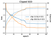
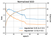
Figure 1: Left: Training loss and training accuracy curves of Clipped SGD. Right: Training loss and training accuracy curves of Normalized SGD. Both are trained with ResNet20 on CIFAR10 task.

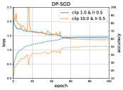
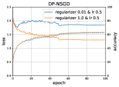
Figure 2: Left: Training loss and training accuracy curves of DP-SGD. Right: Training loss and training accuracy curves of DP-NSGD. Task: ResNet20 on CIFAR10 with $\epsilon=8,\delta=\text{1e-5}$.

However surprisingly, the biases affect the accuracy curves differently for clipped SGD and normalized SGD. The accuracy curves of clipped SGD vary with the value of $c$ while the value of $r$ makes almost no impact on the accuracy curves of normalized SGD. This phenomenon extends to the private setting (look at the accuracy curves in Figure 2).

A qualitative explanation would be as follows. After several epochs of training, good samples $\xi$ (those already been classified correctly) yield small gradients $\nabla\ell({\bm{x}},\xi)$ and bad samples $\xi^{\prime}$ (those not been correctly classified) yield large gradients $\nabla\ell({\bm{x}},\xi^{\prime})$. Typically, $c$ is set on the level of gradient norms, while $r$ is for regularizing the division. As the training goes, the gradient norm becomes small and clipping has no effect on the good samples while normalized SGD comparatively strengthen the effect of good samples. Therefore normalized SGD shows less drop in loss while obtaining a considerable level of accuracy. We call for a future investigation towards understanding this phenomenon thoroughly. Specific to the setting $r\approx 0,c=1$ in Figure 2, normalized SGD normalizes all $\nabla\ell({\bm{x}},\xi)$ to a unit level, while clipped SGD would not change small gradients $\nabla\ell({\bm{x}},\xi)$.

From a theoretical perspective, to give a finer-grained analysis of the bias, imposing further assumptions to control $\gamma$ may be a promising future direction. For example, Chen et al.[12] made an attempt towards this aspect, but their assumption that $\{\nabla\ell({\bm{x}},\xi),\xi\in\mathbb{D}\}$ is nearly symmetric, is a bit artificial and not intuitive. Sankararaman et al.[37] proposed a concept gradient confusion, defined as $\gamma=-\min\{\langle\nabla\ell({\bm{x}},\xi_{i}),\nabla\ell({\bm{x}},\xi_{j})\rangle:i\neq j\}$ to approximately quantify how the per-sample gradients align to each other.

The Added Noises for Privacy Guarantee. For the gradient clipping, the added noise (Gaussian perturbation) $\bar{z}\sim\mathcal{N}(0,c^{2}\sigma^{2}{\bm{I}}_{d})$ is proportional to $c$, while for gradient normalizing $z\sim\mathcal{N}(0,\sigma^{2}{\bm{I}}_{d})$ keeps invariant with $r$. This suggests that when tuning DP-SGD, $\eta$ needs to vary when $c$ changes, in order to control the noise component $\eta\bar{z}$ in each update. In contrast, DP-NSGD is more likely to be robust under different scales of $r$, and thus is easier to tune heuristically. Extensive experiments in Section 4 also support this claim empirically.

4 Experiments

This section conducts experiments to demonstrate the efficacy of Algorithm 1 and compare the behavior of DP-SGD and DP-NSGD empirically. One example for the proof of concept is training a ResNet20 [23] with CIFAR-10 dataset. As in literature [46], we replace all batch normalization layers with group normalization [44] layers for easily computing the per-sample gradients. The non-private accuracy for CIFAR-10 is 90.4%. We compare the performances of DP-NSGD and DP-SGD with a wide range of hyper-parameters and different learning rate scheduling rules. All experiments can be run on a single Tesla V100 with 16GB memory. The ResNet20 has 270K trainable parameters.

Hyperparameter choices. We first fix the privacy budget $\epsilon=\{2.0,4.0,8.0\},\delta=10^{-5}$, which corresponds to setting the noise multiplier $\sigma=\{3.6,2.0,1.2\}$ for the case of batch size 1000 and number of epochs 100 with Rényi differential privacy accountant [1, 31]. There are tighter privacy accountants [22] that can save $\epsilon$ for this noise multiplier. We then fix the weight decay to be 0 and use the classical learning rate scheduling strategy that multiplies the initial $lr$ with $0.1$ at epoch 50 and $0.01$ at epoch 75 respectively. The hyperparameters to tune are the initial learning rate $lr$ and the clip threshold $c$ for DP-SGD [1], where $lr$ takes values $\{0.05,0.1,0.2,0.4,0.8,1.6,3.2\}$ and $c$ takes values $\{0.1,0.4,1.6,6.4,12.8\}$. At the same time, the hyperparameters to tune for DP-NSGD are the initial learning rate $lr$ and the regularizer $r$, where $lr$ takes values $\{0.05,0.1,0.2,0.4,0.8,1.6,3.2\}$ and $r$ takes values $\{0.0001,0.001,0.01,0.1,1.0\}$. We compare the validation accuracy of DP-SGD and DP-NSGD via heatmaps of the above hyperparameter choices in Figure 3. We can see that the performance of DP-NSGD is rather stable for the regularizer taking values from $10^{-4}$ to $1.0$ and it is mostly affected by the learning rate. This is in sharp contrast with the case of DP-SGD where the performance depends on both the learning rate and the clip threshold in a complicated way. This indicates that it is easy to tune the hyperparameters for DP-NSGD, which could not only reduce the tuning effort but also save the privacy budget for tuning hyperparameters [38, 34].

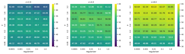
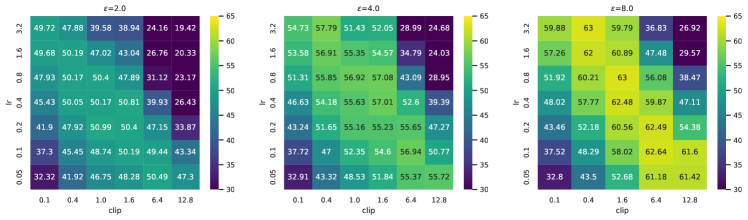
Figure 3: Experiments for ResNet20 on CIFAR10 task. Upper: Accuracy heatmap of DP-NSGD with varying lrs and regularizers. Lower: Accuracy heatmap of DP-SGD with varying lrs and clipping thresholds. The DP parameters are $\delta=1e^{-5}$ and $\epsilon=2.0,4.0,8.0$ from left to right.

We also run the above setting with the cyclic learning rate scheduling with $\text{min-lr}=0.02$ and $\text{max-lr}=1.0$. The best accuracy number are of DP-NSGD and DP-SGD can be as good as 66, which is comparable with the best number that is achieved with model architecture modification in [35].

More experiments on language models are carried out in Appendix D and suggest similar observations.

5 Concluding Remarks

In this paper, we have studied the convergence of two algorithms, i.e., DP-SGD and DP-NSGD, for differentially private non-convex empirical risk minimization. We have achieved a rate that significantly improves over previous literature under similar setup and have analyzed the bias induced by the clipping or normalizing operation. As for future directions, it is very interesting to consider the convergence theorems under stronger assumptions on the gradient distribution.

Appendix A Prerequisite Lemmas

The following is a standard lemma for $(L_{0},L_{1})$-generalized smooth functions, and it can be obtained via Taylor’s expansion. Throughout this appendix, we use $\mathbb{E}_{k}$ to denote taking expectation of $\{{\bm{g}}_{k}^{(i)},i\in\mathcal{S}_{k}\}$ and ${\bm{z}}_{k}$ conditioned on the past, especially ${\bm{x}}_{k}$.

Lemma A.1 (Lemma C.4, [25]).

A function $f:\mathbb{R}^{d}\rightarrow\mathbb{R}^{d}$ is $(L_{0},L_{1})$-generalized smooth, then for any ${\bm{x}},{\bm{x}}^{+}\in\mathbb{R}^{d}$,

$$f({\bm{x}}^{+})\leq f({\bm{x}})+\left\langle\nabla f({\bm{x}}),{\bm{x}}^{+}-{\bm{x}}\right\rangle+\frac{L_{0}+L_{1}\|\nabla f({\bm{x}})\|}{2}\|{\bm{x}}^{+}-{\bm{x}}\|^{2}.$$

Lemma A.2.

For any $k\geq 0$, we use ${\bm{g}}_{k}$ to denote another realization of the underlying distribution behind the set of i.i.d. unbiased estimates $\{{\bm{g}}^{(i)}_{k}:i\in\mathcal{S}_{k}\}$. If we run DP-NSGD iteratively, the trajectory would satisfy the following bound:

$$\mathbb{E}_{k}\left[f({\bm{x}}_{k+1})\right]-f({\bm{x}}_{k})\leq-\eta\mathbb{E}_{k}\left[\langle h_{k}\nabla f({\bm{x}}_{k}),{\bm{g}}_{k}\rangle\right]+\frac{L_{0}+L_{1}\|\nabla f({\bm{x}}_{k})\|}{2}\eta^{2}\left(d\sigma^{2}+\mathbb{E}_{k}\left\|h_{k}{\bm{g}}_{k}\right\|^{2}\right).$$ (12)

Proof.

The updating rule of our iterative algorithm could be summarized as

$${\bm{x}}_{k+1}={\bm{x}}_{k}-\eta\left(\frac{1}{B}\sum_{i\in\mathcal{S}_{k}}h^{(i)}_{k}g^{(i)}_{k}+{\bm{z}}_{k}\right),\quad{\bm{z}}_{k}\sim\mathcal{N}(0,\sigma^{2}{\bm{I}}_{d}).$$

By taking expectation $\mathbb{E}_{k}$ conditioned on the past, we rewrite the first-order term in Lemma A.1 into

$$\mathbb{E}_{k}\left[\left\langle\nabla f({\bm{x}}),{\bm{x}}_{k}-{\bm{x}}_{k+1}\right\rangle\right]=\eta\mathbb{E}_{k}\left[\langle h_{k}\nabla f({\bm{x}}_{k}),{\bm{g}}_{k}\rangle\right].$$ (13)

In the same manner, we bound the second-order term by

$$\mathbb{E}_{k}\|{\bm{x}}_{k+1}-{\bm{x}}_{k}\|^{2}=\eta^{2}d\sigma^{2}+\frac{\eta^{2}}{B^{2}}\mathbb{E}_{k}\left\|\sum_{i\in\mathcal{S}_{k}}h^{(i)}_{k}{\bm{g}}^{(i)}_{k}\right\|^{2}\leq\eta^{2}\left(d\sigma^{2}+\mathbb{E}_{k}\left\|h_{k}{\bm{g}}_{k}\right\|^{2}\right),$$ (14)

where the last inequality follows from an elementary Cauchy-Schwarz inequality,

$$\left\|\sum_{i\in\mathcal{S}_{k}}h^{(i)}_{k}{\bm{g}}^{(i)}_{k}\right\|^{2}\leq B\sum_{i\in\mathcal{S}_{k}}\left\|h^{(i)}_{k}{\bm{g}}^{(i)}_{k}\right\|^{2}.$$

Plug (13) and (14) into Lemma A.1 to obtain the desired result. ∎

Remark A.1.

This lemma implies that mini batch size $B$ does not affect expected upper bounds, due to per-sample gradient normalization. We need to point out that $B$ could still influence high-probability upper bounds, and call for future investigations.

In Section B.1, we will upper bound the second-order term $\frac{L_{0}+L_{1}\|\nabla f({\bm{x}}_{k})\|}{2}\eta^{2}\left(d\sigma^{2}+\mathbb{E}_{k}\left\|h_{k}{\bm{g}}_{k}\right\|^{2}\right)$ by a sum of $\alpha\eta h_{k}\|\nabla f({\bm{x}}_{k})\|$ (for some $0<\alpha<1$) and another term of $\mathcal{O}(\eta^{2})$ via a proper scaling of $\eta$. We firstly present the following lemma to provide a simplified lower bound for the first-order terms

$$\eta\mathbb{E}_{k}\left[\langle h_{k}\nabla f({\bm{x}}_{k}),{\bm{g}}_{k}\rangle\right]-\eta\alpha\mathbb{E}_{k}[h_{k}]\|\nabla f({\bm{x}}_{k})\|^{2}.$$ (15)

Lemma A.3 (Lower bound first-order terms for normalizing).

Define a function $A:\mathbb{R}_{+}\rightarrow\mathbb{R}$ as

$$A(s)=\begin{cases}\left(\dfrac{\tau_{0}}{r(1-\tau_{1})+2\tau_{0}}-\dfrac{\alpha}{1-\tau_{1}}\right)s,&\text{if }s\geq\dfrac{\tau_{0}}{1-\tau_{1}};\\ \dfrac{(1-\alpha)(1-\tau_{1})}{r(1-\tau_{1})+2\tau_{0}}s^{2}-\dfrac{4\tau_{0}^{3}}{r(r+\tau_{0})(1-\tau_{1})^{3}},&\text{otherwise.}\end{cases}$$ (16)

Then we have

$$\eta\mathbb{E}_{k}\left[\langle h_{k}\nabla f({\bm{x}}_{k}),{\bm{g}}_{k}\rangle\right]-\eta\alpha\mathbb{E}_{k}[h_{k}]\|\nabla f({\bm{x}}_{k})\|^{2}\geq\eta A(\|\nabla f({\bm{x}}_{k})\|).$$

Proof.

We prove this lemma via separating the range of $\|\nabla f({\bm{x}}_{k})\|$. When $\|\nabla f({\bm{x}}_{k})\|\geq\tau_{0}/(1-\tau_{1})$, then

$$\langle\nabla f({\bm{x}}_{k}),{\bm{g}}_{k}\rangle=\|\nabla f({\bm{x}}_{k})\|^{2}+\langle\nabla f({\bm{x}}_{k}),{\bm{g}}_{k}-\nabla f({\bm{x}}_{k})\rangle$$

$$\geq (1-\tau_{1})\|\nabla f({\bm{x}}_{k})\|^{2}-\tau_{0}\|\nabla f({\bm{x}}_{k})\|\geq 0,$$

followed by

$$\eta\mathbb{E}_{k}\left[\langle h_{k}\nabla f({\bm{x}}_{k}),{\bm{g}}_{k}\rangle\right]-\eta\alpha\mathbb{E}_{k}[h_{k}]\|\nabla f({\bm{x}}_{k})\|^{2}$$

$$= \mathbb{E}_{k}\left[\frac{\eta\left\langle\nabla f({\bm{x}}_{k}),{\bm{g}}_{k}\right\rangle}{r+\|{\bm{g}}_{k}\|}\right]-\mathbb{E}_{k}\left[\frac{\alpha\eta}{(r+\|{\bm{g}}_{k}\|)}\|\nabla f({\bm{x}}_{k})\|^{2}\right]$$

$$\geq \mathbb{E}_{k}\left[\frac{\eta\left\langle\nabla f({\bm{x}}_{k}),{\bm{g}}_{k}\right\rangle}{r+\tau_{0}+(1+\tau_{1})\|\nabla f({\bm{x}}_{k})\|}\right]-\frac{\alpha}{1-\tau_{1}}\eta\|\nabla f({\bm{x}}_{k})\|$$

$$= \frac{\eta\left\|\nabla f({\bm{x}}_{k})\right\|^{2}}{r+\tau_{0}+(1+\tau_{1})\|\nabla f({\bm{x}}_{k})\|}-\frac{\alpha}{1-\tau_{1}}\eta\|\nabla f({\bm{x}}_{k})\|$$

$$\geq \left(\frac{\tau_{0}}{r(1-\tau_{1})+2\tau_{0}}-\frac{\alpha}{1-\tau_{1}}\right)\eta\|\nabla f({\bm{x}}_{k})\|.$$ (17)

When $\|\nabla f({\bm{x}}_{k})\|<\tau_{0}/(1-\tau_{1})$, we have $\|{\bm{g}}_{k}-\nabla f({\bm{x}}_{k})\|\leq\tau_{0}+\tau_{1}\|\nabla f({\bm{x}}_{k})\|\leq\tau_{0}/(1-\tau_{1})$ as well. Then we decompose the first-order terms by

$$\eta\mathbb{E}_{k}\left[\langle h_{k}\nabla f({\bm{x}}_{k}),{\bm{g}}_{k}\rangle\right]-\eta\alpha\mathbb{E}_{k}[h_{k}]\|\nabla f({\bm{x}}_{k})\|^{2}$$

$$= (1-\alpha)\eta\mathbb{E}_{k}[h_{k}]\|\nabla f({\bm{x}}_{k})\|^{2}+\mathbb{E}_{k}\left[\frac{\eta\left\langle\nabla f({\bm{x}}_{k}),{\bm{g}}_{k}-\nabla f({\bm{x}}_{k})\right\rangle}{r+\|{\bm{g}}_{k}\|}\right].$$

On one hand, we know

$$h_{k}=\frac{1}{r+\|{\bm{g}}_{k}\|}\geq\frac{1}{r+\tau_{0}+(1+\tau_{1})\|\nabla f({\bm{x}}_{k})\|}\geq\frac{1-\tau_{1}}{r(1-\tau_{1})+2\tau_{0}}.$$

On the other hand, we also have

$$\mathbb{E}_{k}\left[\frac{\eta\left\langle\nabla f({\bm{x}}_{k}),{\bm{g}}_{k}-\nabla f({\bm{x}}_{k})\right\rangle}{r+\|{\bm{g}}_{k}\|}\right]$$

$$= \mathbb{E}_{k}\left[\frac{\eta\left\langle\nabla f({\bm{x}}_{k}),{\bm{g}}_{k}-\nabla f({\bm{x}}_{k})\right\rangle}{r+\tau_{0}+(1+\tau_{1})\|\nabla f({\bm{x}}_{k})\|}\right]+\mathbb{E}_{k}\left[\frac{\eta\left[(1+\tau_{1})\|\nabla f({\bm{x}}_{k})\|+\tau_{0}-\|{\bm{g}}_{k}\|\right]\left\langle\nabla f({\bm{x}}_{k}),{\bm{g}}_{k}-\nabla f({\bm{x}}_{k})\right\rangle}{(r+\|{\bm{g}}_{k}\|)(r+\tau_{0}+(1+\tau_{1})\|\nabla f({\bm{x}}_{k})\|)}\right]$$

$$\geq -\eta\frac{4\tau_{0}^{3}}{r(r+\tau_{0})(1-\tau_{1})^{3}}.$$

Therefore, we have

$$\eta\mathbb{E}_{k}\left[\langle h_{k}\nabla f({\bm{x}}_{k}),{\bm{g}}_{k}\rangle\right]-\eta\alpha\mathbb{E}_{k}[h_{k}]\|\nabla f({\bm{x}}_{k})\|^{2}$$

$$\geq \eta\left[\frac{(1-\alpha)(1-\tau_{1})}{r(1-\tau_{1})+2\tau_{0}}\|\nabla f({\bm{x}}_{k})\|^{2}-\frac{4\tau_{0}^{3}}{r(r+\tau_{0})(1-\tau_{1})^{3}}\right].$$ (18)

Combine both cases to derive the required lemma. ∎

We then establish similar results for gradient clipping based algorithms, whose updating rule is described by (2). Firstly, we mimic the proof of Lemma A.2 and derive without proof the following lemma.

Lemma A.4.

For any $k\geq 0$, we use ${\bm{g}}_{k}$ to denote another realization of the underlying distribution behind the set of i.i.d. unbiased estimates $\{{\bm{g}}^{(i)}_{k}:i\in\mathcal{S}_{k}\}$. If we run DP-SGD iteratively, the trajectory would satisfy the following bound:

$$\mathbb{E}_{k}\left[f({\bm{x}}_{k+1})\right]-f({\bm{x}}_{k})\leq-\eta\mathbb{E}_{k}\left[\langle\bar{h}_{k}\nabla f({\bm{x}}_{k}),{\bm{g}}_{k}\rangle\right]+\frac{L_{0}+L_{1}\|\nabla f({\bm{x}}_{k})\|}{2}\eta^{2}\left(dc^{2}\sigma^{2}+\mathbb{E}_{k}\left\|\bar{h}_{k}{\bm{g}}_{k}\right\|^{2}\right).$$ (19)

Then, we provide another lemma for clipping, similar to Lemma A.3.

Lemma A.5 (Lower bound first-order terms for clipping).

Define a function $B:\mathbb{R}_{+}\rightarrow\mathbb{R}$ as

$$B(s)=\begin{cases}\left(\dfrac{\tau_{0}c}{c(1-\tau_{1})+2\tau_{0}}-\dfrac{\alpha}{1-\tau_{1}}\right)s,&\text{if }s\geq\dfrac{\tau_{0}}{1-\tau_{1}};\\ (1-\alpha)s^{2},&\text{otherwise.}\end{cases}$$ (20)

If we take $c\geq 2\tau_{0}/(1-\tau_{1})$, then

$$\eta\mathbb{E}_{k}\left[\langle\bar{h}_{k}\nabla f({\bm{x}}_{k}),{\bm{g}}_{k}\rangle\right]-\eta\alpha\mathbb{E}_{k}[\bar{h}_{k}]\|\nabla f({\bm{x}}_{k})\|^{2}\geq\eta B(\|\nabla f({\bm{x}}_{k})\|).$$

Proof.

Recall that $\bar{h}_{k}$ is defined as

$$\bar{h}_{k}=\min\left\{1,\frac{c}{\|{\bm{g}}_{k}\|}\right\}\geq\frac{c}{c+\|{\bm{g}}_{k}\|}.$$

Again, we take the strategy of separting the range of $\|\nabla f({\bm{x}}_{k})\|$. When $\|\nabla f({\bm{x}}_{k})\|\geq\tau_{0}/(1-\tau_{1})$, we know $\left\langle\nabla f({\bm{x}}_{k}),{\bm{g}}_{k}\right\rangle\geq 0$, followed by

$$\eta\mathbb{E}_{k}\left[\langle\bar{h}_{k}\nabla f({\bm{x}}_{k}),{\bm{g}}_{k}\rangle\right]-\eta\alpha\mathbb{E}_{k}[\bar{h}_{k}]\|\nabla f({\bm{x}}_{k})\|^{2}$$

$$\geq \mathbb{E}_{k}\left[\frac{\eta c\left\langle\nabla f({\bm{x}}_{k}),{\bm{g}}_{k}\right\rangle}{c+\|{\bm{g}}_{k}\|}\right]-\mathbb{E}_{k}\left[\frac{\alpha\eta}{\|{\bm{g}}_{k}\|}\|\nabla f({\bm{x}}_{k})\|^{2}\right]$$

$$\geq \mathbb{E}_{k}\left[\frac{\eta c\left\langle\nabla f({\bm{x}}_{k}),{\bm{g}}_{k}\right\rangle}{c+\tau_{0}+(1+\tau_{1})\|\nabla f({\bm{x}}_{k})\|}\right]-\frac{\alpha}{1-\tau_{1}}\eta\|\nabla f({\bm{x}}_{k})\|$$

$$= \frac{\eta c\left\|\nabla f({\bm{x}}_{k})\right\|^{2}}{c+\tau_{0}+(1+\tau_{1})\|\nabla f({\bm{x}}_{k})\|}-\frac{\alpha}{1-\tau_{1}}\eta\|\nabla f({\bm{x}}_{k})\|$$

$$\geq \left(\frac{\tau_{0}c}{c(1-\tau_{1})+2\tau_{0}}-\frac{\alpha}{1-\tau_{1}}\right)\eta\|\nabla f({\bm{x}}_{k})\|.$$

Otherwise, when $\|\nabla f({\bm{x}}_{k})\|<\tau_{0}/(1-\tau_{1})\leq(c-\tau_{0})/(1+\tau_{1})$ where the second inequality follows from $c\geq 2\tau_{0}/(1-\tau_{1})$, we know

$$\|{\bm{g}}_{k}\|\leq\tau_{0}+(1+\tau_{1})\|\nabla f({\bm{x}}_{k})\|\leq c.$$

Therefore in this case, $\bar{h}_{k}=1$ and

$$\eta\mathbb{E}_{k}\left[\langle\bar{h}_{k}\nabla f({\bm{x}}_{k}),{\bm{g}}_{k}\rangle\right]-\eta\alpha\mathbb{E}_{k}[\bar{h}_{k}]\|\nabla f({\bm{x}}_{k})\|^{2}=(1-\alpha)\eta\|\nabla f({\bm{x}}_{k})\|^{2}.$$

Combine both cases to conclude the desired lemma. ∎

A.1 Toy Example

Followed from the discussion in Subsection 3.3, a toy example is to presented here further illustrate the different behavior of $\mathfrak{A}:=\eta\mathbb{E}\left[\langle\nabla f,h{\bm{g}}\rangle\right]$ and $\bar{\mathfrak{A}}:=\eta\mathbb{E}\left[\langle\nabla f,\bar{h}{\bm{g}}\rangle\right]$. Assign this simple distribution to ${\bm{e}}\triangleq{\bm{g}}-\nabla f$:

$$\mathbb{P}\left({\bm{e}}=\frac{\tau_{0}\nabla f}{\|\nabla f\|}\right)=\frac{1}{3},\;\;\;\mathbb{P}\left({\bm{e}}=-\frac{\tau_{0}\nabla f}{2\|\nabla f\|}\right)=\frac{2}{3}.$$

This distribution certainly satisfies Assumption 2.2 with $\tau_{1}=0$. We calculate the explicit formula of $\mathfrak{A}$ for this toy example

$$\mathfrak{A}=\frac{\eta(\|\nabla f\|^{3}+(3r+\tau_{0}/2)\|\nabla f\|^{2}-\tau_{0}^{2}\|\nabla f\|/2)}{3(r+\tau_{0}+\|\nabla f\|)(r+\tau_{0}/2-\|\nabla f\|)}.$$

For $\|\nabla f({\bm{x}}_{k})\|\leq\tau_{0}^{2}/(10r)$, we can compute $\mathfrak{A}<0$. It implies that the function value may not even decrease along $\mathbb{E}[h{\bm{g}}]$ in this case and the learning curves are expected to fluctuate adversely. This toy example also supports that the lower bound $\mathfrak{A}=\Omega\left(\eta\left(\|\nabla f\|^{2}/r-\tau_{0}^{3}/r^{2}\right)\right)$ we derived is optimal. In contrast for the clipping operation, as long as $\|\nabla f\|\leq c-\tau_{0}$, we have $\bar{h}\equiv 1$ and therefore $\bar{\mathfrak{A}}=\eta\|\nabla f\|^{2}$.

Appendix B Proofs for DP-NSGD

In this section, we provide a rigorous convergence theory for normalized stochastic gradient descent with perturbation. Unavoidable error between ${\bm{g}}_{k}$ and $\nabla f({\bm{x}}_{k})$ is a central distinction between stochastic and deterministic optimization methods. We begin with an explicit decomposition for (12)

$$\mathbb{E}_{k}\left[f({\bm{x}}_{k+1})\right]-f({\bm{x}}_{k})\leq -\eta\mathbb{E}_{k}\left[h_{k}\right]\|\nabla f({\bm{x}}_{k})\|^{2}-\eta\mathbb{E}_{k}\left[\langle h_{k}\nabla f({\bm{x}}_{k}),{\bm{g}}_{k}-\nabla f({\bm{x}}_{k})\rangle\right]$$

$$+\frac{L_{0}+L_{1}\|\nabla f({\bm{x}}_{k})\|}{2}\eta^{2}\left(\mathbb{E}_{k}\left[h_{k}^{2}\left\|\nabla f({\bm{x}}_{k})\right\|^{2}\right]+2\mathbb{E}_{k}\left[h_{k}^{2}\langle{\bm{g}}_{k}-\nabla f({\bm{x}}_{k}),\nabla f({\bm{x}}_{k})\rangle\right]\right)$$

$$+\frac{L_{0}+L_{1}\|\nabla f({\bm{x}}_{k})\|}{2}\eta^{2}\left(d\sigma^{2}+\mathbb{E}_{k}\left[h_{k}^{2}\left\|{\bm{g}}_{k}-\nabla f({\bm{x}}_{k})\right\|^{2}\right]\right).$$ (21)

B.1 Upper Bound Second-order Terms

In theory, we need to carefully distinguish these terms accourding to their orders of $\eta$, as the first order term $\mathbb{E}_{k}\left[\langle h_{k}\nabla f({\bm{x}}_{k}),{\bm{g}}_{k}\rangle\right]$ controls the amount of descent mainly. We show that the second order terms could be bounded by first order terms via a proper scaling of $\eta$, in the following technical lemma.

Lemma B.1.

For any $0<\alpha<1$ to be determined explicitly later, if

$$\eta\leq\min\left(\dfrac{(r-\tau_{0})\alpha}{4L_{0}},\dfrac{(1-\tau_{1})\alpha}{4L_{1}},\dfrac{\alpha}{6L_{1}d\sigma^{2}}\right)$$ (22)

then we have

$$\frac{L_{0}+L_{1}\|\nabla f({\bm{x}}_{k})\|}{2}\eta^{2}d\sigma^{2}\leq \frac{L_{0}+L_{1}(r+\tau_{0})}{2}\eta^{2}d\sigma^{2}+\frac{\alpha\eta h_{k}}{4}\|\nabla f({\bm{x}}_{k})\|^{2},$$ (23)

$$(L_{0}+L_{1}\|\nabla f({\bm{x}}_{k})\|)\eta^{2}h_{k}^{2}\langle\nabla f({\bm{x}}_{k}),{\bm{g}}_{k}-\nabla f({\bm{x}}_{k})\rangle\leq \frac{(L_{0}(1-\tau_{1})+L_{1}\tau_{0})\tau_{0}^{2}}{r^{2}(1-\tau_{1})^{3}}\eta^{2}+\frac{\alpha\eta h_{k}}{4}\|\nabla f({\bm{x}}_{k})\|^{2},$$ (24)

$$\frac{L_{0}+L_{1}\|\nabla f({\bm{x}}_{k})\|}{2}\eta^{2}h_{k}^{2}\|{\bm{g}}_{k}-\nabla f({\bm{x}}_{k})\|^{2}\leq \frac{(L_{0}(1-\tau_{1})+L_{1}\tau_{0})\tau_{0}^{2}}{2r^{2}(1-\tau_{1})^{3}}\eta^{2}+\frac{\alpha\eta h_{k}}{4}\|\nabla f({\bm{x}}_{k})\|^{2},$$ (25)

$$\frac{L_{0}+L_{1}\|\nabla f({\bm{x}}_{k})\|}{2}\eta^{2}h_{k}^{2}\|\nabla f({\bm{x}}_{k})\|^{2}\leq \frac{\alpha\eta h_{k}}{4}\|\nabla f({\bm{x}}_{k})\|^{2}.$$ (26)

Remark B.1.

These bounds are proved by separating the range of $\|\nabla f({\bm{x}}_{k})\|$. When it is smaller than some threshold, we can obtain an upper bound of $\mathcal{O}(\eta^{2})$. Otherwise, when $\|\nabla f({\bm{x}}_{k})\|$ is greater than the threshold, $h_{k}$ is of order $\Omega(1/\|\nabla f({\bm{x}}_{k})\|)$, then the left hand terms are all of order $\mathcal{O}(\eta^{2}h_{k}\|f({\bm{x}})\|^{2})$. Therefore we scale $\eta$ small enough to make left hand terms smaller than $\alpha\eta h_{k}\|f({\bm{x}})\|^{2}/4$. At last, we sum up the respective upper bounds together to conclude the lemma.

Remark B.2.

Moreover, we remark that the thresholds chosen during proof ($r+\tau_{0}$ for proving (23) and $\tau_{0}/(1-\tau_{1})$ for proving (24) and (25)) are quite artificial. A thorough investigation towards these thresholds would definitely improve the dependence on the constants $(L_{0},L_{1},\tau_{0},\tau_{1})$, but would not affect our main argument.

Proof.

In fact, this lemma can be proved in an obvious way by separating into different cases.

(i)

If $\|\nabla f({\bm{x}}_{k})\|\leq r+\tau_{0}$, it directly follows that $L_{1}\|\nabla f({\bm{x}}_{k})\|\eta^{2}d\sigma^{2}/2\leq L_{1}(r+\tau_{0})\eta^{2}d\sigma^{2}/2$; otherwise, if $\|\nabla f({\bm{x}}_{k})\|>r+\tau_{0}$, we know

$$h_{k}=\frac{1}{r+\|{\bm{g}}_{k}\|}\geq\frac{1}{r+\tau_{0}+(\tau_{1}+1)\|\nabla f({\bm{x}}_{k})\|}\geq\frac{1}{3\|\nabla f({\bm{x}}_{k})\|},$$

therefore $\eta\leq\alpha/(6L_{1}d\sigma^{2})$ directly yields

$$\frac{L_{1}\|\nabla f({\bm{x}}_{k})\|\eta^{2}d\sigma^{2}}{2}\leq\frac{\eta\alpha h_{k}\|\nabla f({\bm{x}}_{k})\|^{2}}{4}.$$

Then (23) follows from summing up these two cases.

(ii)

If $\|\nabla f({\bm{x}}_{k})\|\leq\tau_{0}/(1-\tau_{1})$, then $\|{\bm{g}}_{k}-\nabla f({\bm{x}}_{k})\|\leq\tau_{0}+\tau_{1}\|\nabla f({\bm{x}}_{k})\|\leq\tau_{0}/(1-\tau_{1})$ and $h_{k}\leq 1/r$, which yield

$$(L_{0}+L_{1}\|\nabla f({\bm{x}}_{k})\|)\eta^{2}h_{k}^{2}\langle\nabla f({\bm{x}}_{k}),{\bm{g}}_{k}-\nabla f({\bm{x}}_{k})\rangle\leq \frac{(L_{0}(1-\tau_{1})+L_{1}\tau_{0})\tau_{0}^{2}}{r^{2}(1-\tau_{1})^{3}}\eta^{2},$$

$$\frac{L_{0}+L_{1}\|\nabla f({\bm{x}}_{k})\|}{2}\eta^{2}h_{k}^{2}\|{\bm{g}}_{k}-\nabla f({\bm{x}}_{k})\|^{2}\leq \frac{(L_{0}(1-\tau_{1})+L_{1}\tau_{0})\tau_{0}^{2}}{2r^{2}(1-\tau_{1})^{3}}\eta^{2}.$$

Otherwise, if $\|\nabla f({\bm{x}}_{k})\|>\tau_{0}/(1-\tau_{1})$, we note that $\|{\bm{g}}_{k}\|\geq-\tau_{0}+(1-\tau_{1})\|\nabla f({\bm{x}}_{k})\|$ and

$$h_{k}(L_{0}+L_{1}\|\nabla f({\bm{x}}_{k})\|)\leq\frac{L_{0}+L_{1}\|\nabla f({\bm{x}}_{k})\|}{r-\tau_{0}+(1-\tau_{1})\|\nabla f({\bm{x}}_{k})\|}\leq\max\left(\frac{L_{0}}{r-\tau_{0}},\frac{L_{1}}{1-\tau_{1}}\right).$$

Consequently, once $\eta\leq\dfrac{\alpha}{4}\min\left(\dfrac{r-\tau_{0}}{L_{0}},\dfrac{1-\tau_{1}}{L_{1}}\right)$, we have

$$(L_{0}+L_{1}\|\nabla f({\bm{x}}_{k})\|)\eta^{2}h_{k}^{2}\langle\nabla f({\bm{x}}_{k}),{\bm{g}}_{k}-\nabla f({\bm{x}}_{k})\rangle$$

$$\leq \max\left(\frac{L_{0}}{r-\tau_{0}},\frac{L_{1}}{1-\tau_{1}}\right)\eta^{2}h_{k}\|\nabla f({\bm{x}}_{k})\|^{2}\leq\frac{\eta\alpha h_{k}}{4}\|\nabla f({\bm{x}}_{k})\|^{2},$$

and

$$\frac{L_{0}+L_{1}\|\nabla f({\bm{x}}_{k})\|}{2}\eta^{2}h_{k}^{2}\|{\bm{g}}_{k}-\nabla f({\bm{x}}_{k})\|^{2}$$

$$\leq \frac{1}{2}\max\left(\frac{L_{0}}{r-\tau_{0}},\frac{L_{1}}{1-\tau_{1}}\right)\eta^{2}h_{k}\|\nabla f({\bm{x}}_{k})\|^{2}\leq\frac{\eta\alpha h_{k}}{4}\|\nabla f({\bm{x}}_{k})\|^{2}.$$

We obtain (24) and (25) via summing up respective bounds for two cases.

(iii)

The last bound (26) can be derived directly by

$$\frac{L_{0}+L_{1}\|\nabla f({\bm{x}}_{k})\|}{2}\eta^{2}h_{k}^{2}\|\nabla f({\bm{x}}_{k})\|^{2}\leq\max\left(\frac{L_{0}}{r-\tau_{0}},\frac{L_{1}}{\tau_{1}}\right)\frac{\eta^{2}}{2}h_{k}\|\nabla f({\bm{x}}_{k})\|^{2}\leq\frac{\eta\alpha h_{k}}{4}\|\nabla f({\bm{x}}_{k})\|^{2}$$

via setting $\eta\leq\dfrac{\alpha}{2}\min\left(\dfrac{r-\tau_{0}}{L_{0}},\dfrac{\tau_{1}}{L_{1}}\right)$.

In conclusion, it suffices to set $\eta\leq\min\left(\dfrac{(r-\tau_{0})\alpha}{4L_{0}},\dfrac{(1-\tau_{1})\alpha}{4L_{1}},\dfrac{\alpha}{6L_{1}d\sigma^{2}}\right)$ to obtain these bounds. ∎

In the sequel, we will use this lemma only with

$$\alpha=\alpha_{0}:=\frac{\tau_{0}(1-\tau_{1})}{2r(1-\tau_{1})+4\tau_{0}}<\frac{1}{4}$$ (27)

Lemma B.2.

In the statement of Theorem 3.2, we take $\eta=\sqrt{\frac{2}{L_{1}(r+\tau_{0})Td\sigma^{2}}}$. Then the condition (22) in Lemma B.1 holds as long as we run the algorithm long enough i.e. $T\geq C\left(\sigma^{2},\tau,L,d,r\right)$.

Proof.

We see that

$$\eta=\sqrt{\frac{2}{L_{1}(r+\tau_{0})Td\sigma^{2}}}\leq\min\left(\dfrac{(r-\tau_{0})\alpha_{0}}{4L_{0}},\dfrac{(1-\tau_{1})^{2}\alpha_{0}}{4L_{1}},\dfrac{\alpha_{0}}{6L_{1}d\sigma^{2}}\right)$$

is equivalent to

$$T\geq\max\left(\dfrac{32L_{0}^{2}}{(r-\tau_{0})^{2}\alpha_{0}^{2}L_{1}(r+\tau_{0})d\sigma^{2}},\dfrac{32L_{1}}{\tau_{1}^{2}\alpha_{0}^{2}(r+\tau_{0})d\sigma^{2}},\dfrac{72L_{1}d}{\alpha_{0}^{2}(r+\tau_{0})}\right).$$

∎

B.2 Final Procedures in Proof

Proof of Theorem 3.2.

Equipped with Lemmas A.3 ,B.1 and B.3, we further wrote the one step inequality (21) into

$$\eta A(\|\nabla f({\bm{x}}_{k})\|)\leq f({\bm{x}}_{k})-\mathbb{E}_{k}\left[f({\bm{x}}_{k+1})\right]$$

$$+\eta^{2}\left(\frac{(L_{1}(r+\tau_{0})+L_{0})d\sigma^{2}}{2}+\frac{3(L_{0}(1-\tau_{1})+L_{1}\tau_{0})\tau_{0}^{2}}{2r^{2}(1-\tau_{1})^{3}}\eta^{2}\right).$$ (28)

We then separate the time index into

$$\mathcal{U}=\left\{k<T:\|\nabla f({\bm{x}}_{k})\|\geq\frac{\tau_{0}}{1-\tau_{1}}\right\}$$

and $\mathcal{U}^{c}=\{0,1,\cdots,T-1\}\backslash\mathcal{U}$. Given this, we derive from (17) that for any $k\in\mathcal{U}$,

$$\frac{\tau_{0}}{2r(1-\tau_{1})+4\tau_{0}}\eta\|\nabla f({\bm{x}}_{k})\|$$

$$\leq \mathbb{E}_{k}\left[f({\bm{x}}_{k+1})\right]-f({\bm{x}}_{k})+\eta^{2}\left(\frac{(L_{1}(r+\tau_{0})+L_{0})d\sigma^{2}}{2}+\frac{3(L_{0}(1-\tau_{1})+L_{1}\tau_{0})\tau_{0}^{2}}{2r^{2}(1-\tau_{1})^{3}}\right).$$

Similarly, together with $\alpha_{0}\leq 1/4$, (18) deduces that for any $k\in\mathcal{U}^{c}$,

$$\eta\left[\frac{3(1-\tau_{1})}{4r(1-\tau_{1})+8\tau_{0}}\|\nabla f({\bm{x}}_{k})\|^{2}-\frac{4\tau_{0}^{3}}{r(r+\tau_{0})(1-\tau_{1})^{3}}\right]$$

$$\leq \mathbb{E}_{k}\left[f({\bm{x}}_{k+1})\right]-f({\bm{x}}_{k})+\eta^{2}\left(\frac{(L_{1}(r+\tau_{0})+L_{0})d\sigma^{2}}{2}+\frac{3(L_{0}(1-\tau_{1})+L_{1}\tau_{0})\tau_{0}^{2}}{2r^{2}(1-\tau_{1})^{3}}\right).$$

Sum these inequalities altogether to have

$$\frac{1}{r+2\tau_{0}}\max\left\{\frac{\tau_{0}}{2T}\sum_{k\in\mathcal{U}}\|\nabla f({\bm{x}}_{k})\|,\frac{3(1-\tau_{1})}{4T}\sum_{k\notin\mathcal{U}}\|\nabla f({\bm{x}}_{k})\|^{2}\right\}$$

$$\leq \frac{D_{f}}{T\eta}+\eta\frac{(L_{1}(r+\tau_{0})+L_{0})d\sigma^{2}}{2}+\eta\frac{3(L_{0}(1-\tau_{1})+L_{1}\tau_{0})\tau_{0}^{2}}{2r^{2}(1-\tau_{1})^{3}}+\frac{4\tau_{0}^{3}}{r(r+\tau_{0})(1-\tau_{1})^{3}}\frac{|\mathcal{U}^{c}|}{T}.$$

We set

$$\eta=\sqrt{\frac{2}{(L_{1}(r+\tau_{0})+L_{0})Td\sigma^{2}}}.$$ (29)

We then define

$$\Delta=(D_{f}+1)\sqrt{\frac{(L_{1}(r+\tau_{0})+L_{0})d\sigma^{2}}{2T}}+\frac{3(L_{0}+L_{1}\tau_{0})\tau_{0}^{2}}{2r^{2}(1-\tau_{1})^{3}}\sqrt{\frac{2}{(L_{1}(r+\tau_{0})+L_{0})Td\sigma^{2}}}+\frac{4\tau_{0}^{3}}{r(r+\tau_{0})(1-\tau_{1})^{3}}.$$ (30)

Recall that $\sigma^{2}$ can have some dependence on $T$, so actually these three terms are $\mathcal{O}(\sigma/\sqrt{T}),\mathcal{O}(1/(\sqrt{T}\sigma))$ and $\mathcal{O}(1)$ respectively. Then we further have

$$\mathbb{E}\left[\min_{0\leq k<T}\|\nabla f({\bm{x}}_{k})\|\right]$$

$$\leq \mathbb{E}\left[\min\left\{\sqrt{\dfrac{1}{|\mathcal{U}|}\sum_{k\in\mathcal{U}^{c}}\|\nabla f({\bm{x}}_{k})\|^{2}},\dfrac{1}{|\mathcal{U}|}\sum_{k\notin\mathcal{U}}\|\nabla f({\bm{x}}_{k})\|\right\}\right]$$

$$\leq \max\left\{\sqrt{\dfrac{8(r+2\tau_{0})}{3(1-\tau_{1})}\Delta},\dfrac{2(r+2\tau_{0})}{\tau_{0}}\Delta\right\},$$ (31)

where the second inequality follows from the fact that either $|\mathcal{U}|\geq T/2$ or $|\mathcal{U}^{c}|\geq T/2$. In the end, we capture the leading terms in this upper bound to have

$$\mathbb{E}\left[\min_{0\leq k<T}\|\nabla f({\bm{x}}_{k})\|\right]\leq\mathcal{O}\left(\sqrt[4]{\frac{(D_{f}+1)^{2}(L_{1}(r+\tau_{0})+L_{0})(r+2\tau_{0})^{2}d\sigma^{2}}{T(1-\tau_{1})^{2}}}\right)$$

$$+\mathcal{O}\left(\sqrt{\sqrt{\frac{2(r+2\tau_{0})^{2}}{(L_{1}(r+\tau_{0})+L_{0})Td\sigma^{2}}}\frac{3(L_{0}+L_{1}\tau_{0})\tau_{0}^{2}}{2r^{2}(1-\tau_{1})^{4}}}+\frac{8(r+2\tau_{0})\tau_{0}^{2}}{r(r+\tau_{0})(1-\tau_{1})^{3}}\right).$$

∎

Lemma B.3.

In the statement of Corollary 3.3, we take $\eta=\sqrt{\frac{2}{(L_{1}(r+\tau_{0})+L_{0})Td\sigma^{2}}}$, $\sigma=c_{2}B\sqrt{T\log\frac{1}{\delta}}/(N\epsilon)$ and $T\geq{\mathcal{O}}(N^{2}\epsilon^{2}/(B^{2}r^{3}d\log\frac{1}{\delta}))$. Then the condition in Lemma B.2 holds as long as we have enough samples i.e. $N\geq L_{1}C\left(\epsilon,\delta,\tau,L,B,d,r\right)$.

Proof.

It is more straight-forward to verify the condition (22) directly. Firstly, we plug $\sigma^{2}=\frac{c_{2}^{2}B^{2}T\log(1/\delta)}{N^{2}\epsilon^{2}}$ from Lemma 3.1 into the formula of $\eta$ to have

$$\eta=\sqrt{\frac{2}{(L_{1}(r+\tau_{0})+L_{0})Td\sigma^{2}}}=\frac{N\epsilon}{c_{2}BT}\sqrt{\frac{2}{(L_{1}(r+\tau_{0})+L_{0})d\log(1/\delta)}}\leq\frac{\alpha_{0}N^{2}\epsilon^{2}}{6L_{1}dc_{2}^{2}B^{2}T\log(1/\delta)}=\frac{\alpha_{0}}{6L_{1}d\sigma^{2}}$$

as long as we have enough samples

$$N\geq\frac{6c_{2}BL_{1}}{\epsilon\alpha_{0}}\sqrt{\frac{2d\log(1/\delta)}{L_{1}(r+\tau_{0})+L_{0}}}.$$

Other conditions

$$\eta=\frac{N\epsilon}{c_{2}BT}\sqrt{\frac{2}{(L_{1}(r+\tau_{0})+L_{0})d\log(1/\delta)}}\leq\min\left\{\dfrac{(r-\tau_{0})\alpha_{0}}{4L_{0}},\dfrac{(1-\tau_{1})\alpha_{0}}{4L_{1}}\right\}$$

holds as long as we run the algorithm long enough

$$\frac{T}{N}\geq\min\left\{\dfrac{L_{0}}{r-\tau_{0}},\dfrac{L_{1}}{\tau_{1}}\right\}\frac{4\epsilon}{\alpha_{0}c_{2}B}\sqrt{\frac{2}{(L_{1}(r+\tau_{0})+L_{0})d\log(1/\delta)}}.$$ (32)

The last requirement (32) naturally holds due to $T\geq{\mathcal{O}}(N^{2}\epsilon^{2}/(B^{2}r^{3}d\log\frac{1}{\delta}))$. ∎

Proof of Corollary 3.3.

Moreover, we take the limit $T\geq{\mathcal{O}}(N^{2}\epsilon^{2}/(B^{2}r^{3}d\log\frac{1}{\delta}))$ to derive the privacy-utility trade-off

$$\mathbb{E}\left[\min_{0\leq k<T}\|\nabla f({\bm{x}}_{k})\|\right]\leq\mathcal{O}\left(\sqrt[4]{\frac{(D_{f}+1)^{2}(L_{1}(r+\tau_{0})+L_{0})dB^{2}\log(1/\delta)}{N^{2}\epsilon^{2}}}+\frac{8(r+2\tau_{0})\tau_{0}^{3}}{r(r+\tau_{0})(1-\tau_{1})^{3}}\right),$$

ending the proof. ∎

Appendix C Proofs for DP-SGD

In this section, we prove the convergence theorem for DP-SGD following the roadmap outlined in Section B. To start with, we extend (19) into

$$\mathbb{E}_{k}\left[f({\bm{x}}_{k+1})\right]-f({\bm{x}}_{k})\leq -\eta\mathbb{E}_{k}\left[\bar{h}_{k}\right]\|\nabla f({\bm{x}}_{k})\|^{2}-\eta\mathbb{E}_{k}\left[\langle\bar{h}_{k}\nabla f({\bm{x}}_{k}),{\bm{g}}_{k}-\nabla f({\bm{x}}_{k})\rangle\right]$$

$$+\frac{L_{0}+L_{1}\|\nabla f({\bm{x}}_{k})\|}{2}\eta^{2}\left(\mathbb{E}_{k}\left[\bar{h}_{k}^{2}\left\|\nabla f({\bm{x}}_{k})\right\|^{2}\right]+2\mathbb{E}_{k}\left[\bar{h}_{k}^{2}\langle{\bm{g}}_{k}-\nabla f({\bm{x}}_{k}),\nabla f({\bm{x}}_{k})\rangle\right]\right)$$

$$+\frac{L_{0}+L_{1}\|\nabla f({\bm{x}}_{k})\|}{2}\eta^{2}\left(dc^{2}\sigma^{2}+\mathbb{E}_{k}\left[\bar{h}_{k}^{2}\left\|{\bm{g}}_{k}-\nabla f({\bm{x}}_{k})\right\|^{2}\right]\right).$$ (33)

C.1 Upper Bound Second-order Terms

In the same spirit as Lemma B.1, we provide an upper bound for the second-order terms in the following lemma.

Lemma C.1.

For any $0<\alpha<1$ to be determined explicitly later, if

$$\eta\leq\min\left\{\dfrac{\alpha}{6L_{1}dc\sigma^{2}},\dfrac{\alpha(1-\tau_{1})}{2L_{0}(1-\tau_{1})+4L_{1}\tau_{0}},\dfrac{\alpha\tau_{0}(1-\tau_{1})}{4c(L_{0}(1-\tau_{1})+2L_{1}\tau_{0})}\right\},$$ (34)

then we have

$$\frac{L_{0}+L_{1}\|\nabla f({\bm{x}}_{k})\|}{2}\eta^{2}dc^{2}\sigma^{2}\leq \frac{L_{1}(c+\tau_{0})+L_{0}}{2}\eta^{2}dc^{2}\sigma^{2}+\frac{\alpha\eta\bar{h}_{k}}{4}\|\nabla f({\bm{x}}_{k})\|^{2},$$ (35)

$$(L_{0}+L_{1}\|\nabla f({\bm{x}}_{k})\|)\eta^{2}\bar{h}_{k}^{2}\langle\nabla f({\bm{x}}_{k}),{\bm{g}}_{k}-\nabla f({\bm{x}}_{k})\rangle\leq \frac{2(L_{0}(1-\tau_{1})+2L_{1}\tau_{0})\tau_{0}^{2}}{(1-\tau_{1})^{3}}\eta^{2}+\frac{\alpha\eta\bar{h}_{k}}{4}\|\nabla f({\bm{x}}_{k})\|^{2},$$ (36)

$$\frac{L_{0}+L_{1}\|\nabla f({\bm{x}}_{k})\|}{2}\eta^{2}\bar{h}_{k}^{2}\|{\bm{g}}_{k}-\nabla f({\bm{x}}_{k})\|^{2}\leq \frac{2(L_{0}(1-\tau_{1})+2L_{1}\tau_{0})\tau_{0}^{2}}{(1-\tau_{1})^{3}}\eta^{2}+\frac{\alpha\eta\bar{h}_{k}}{4}\|\nabla f({\bm{x}}_{k})\|^{2},$$ (37)

$$\frac{L_{0}+L_{1}\|\nabla f({\bm{x}}_{k})\|}{2}\eta^{2}\bar{h}_{k}^{2}\|\nabla f({\bm{x}}_{k})\|^{2}\leq \frac{\alpha\eta\bar{h}_{k}}{4}\|\nabla f({\bm{x}}_{k})\|^{2}.$$ (38)

Proof.

In fact, this lemma can be proved in an obvious way by separating into different cases.

(i)

If $\|\nabla f({\bm{x}}_{k})\|\leq c+\tau_{0}$, it directly follows that $L_{1}\|\nabla f({\bm{x}}_{k})\|\eta^{2}d\sigma^{2}/2\leq L_{1}(c+\tau_{0})\eta^{2}dc^{2}\sigma^{2}/2$; otherwise, if $\|\nabla f({\bm{x}}_{k})\|>c+\tau_{0}$, we know

$$\bar{h}_{k}=\min\left\{1,\frac{c}{\|{\bm{g}}_{k}\|}\right\}\geq\frac{c}{c+\|{\bm{g}}_{k}\|}\geq\frac{c}{c+\tau_{0}+(\tau_{1}+1)\|\nabla f({\bm{x}}_{k})\|}\geq\frac{c}{3\|\nabla f({\bm{x}}_{k})\|}$$

therefore $\eta\leq\alpha/(6L_{1}dc\sigma^{2})$ directly yields

$$\frac{L_{1}\|\nabla f({\bm{x}}_{k})\|\eta^{2}dc^{2}\sigma^{2}}{2}\leq\frac{\eta\alpha\bar{h}_{k}\|\nabla f({\bm{x}}_{k})\|^{2}}{4}.$$

Then (35) follows from summing up these two cases.

(ii)

If $\|\nabla f({\bm{x}}_{k})\|\leq 2\tau_{0}/(1-\tau_{1})$, then $\|{\bm{g}}_{k}-\nabla f({\bm{x}}_{k})\|\leq\tau_{0}+\tau_{1}\|\nabla f({\bm{x}}_{k})\|\leq 2\tau_{0}/(1-\tau_{1})$ and $\bar{h}_{k}\leq 1$, which yield

$$(L_{0}+L_{1}\|\nabla f({\bm{x}}_{k})\|)\eta^{2}\bar{h}_{k}^{2}\langle\nabla f({\bm{x}}_{k}),{\bm{g}}_{k}-\nabla f({\bm{x}}_{k})\rangle\leq \frac{2(L_{0}(1-\tau_{1})+2L_{1}\tau_{0})\tau_{0}^{2}}{(1-\tau_{1})^{3}}\eta^{2},$$

$$\frac{L_{0}+L_{1}\|\nabla f({\bm{x}}_{k})\|}{2}\eta^{2}\bar{h}_{k}^{2}\|{\bm{g}}_{k}-\nabla f({\bm{x}}_{k})\|^{2}\leq \frac{2(L_{0}(1-\tau_{1})+2L_{1}\tau_{0})\tau_{0}^{2}}{(1-\tau_{1})^{3}}\eta^{2}.$$

Otherwise, if $\|\nabla f({\bm{x}}_{k})\|>2\tau_{0}/(1-\tau_{1})$, we note that $\|{\bm{g}}_{k}-\nabla f({\bm{x}}_{k})\|\leq\frac{1+\tau_{1}}{2}\|\nabla f({\bm{x}}_{k})\|$ and $\|{\bm{g}}_{k}\|\geq\frac{1-\tau_{1}}{2}\|\nabla f({\bm{x}}_{k})\|$. Moreover,

$$\bar{h}_{k}(L_{0}+L_{1}\|\nabla f({\bm{x}}_{k})\|)\leq\frac{c(L_{0}+L_{1}\|\nabla f({\bm{x}}_{k})\|))}{\|{\bm{g}}_{k}\|}\leq\frac{2c(L_{0}+L_{1}\|\nabla f({\bm{x}}_{k})\|))}{(1-\tau_{1})\|\nabla f({\bm{x}}_{k})\|}\leq\frac{cL_{0}}{\tau_{0}}+\frac{2cL_{1}}{1-\tau_{1}}.$$

Consequently, once $\eta\leq\dfrac{\alpha}{4}\dfrac{\tau_{0}(1-\tau_{1})}{c(L_{0}(1-\tau_{1})+2L_{1}\tau_{0})}$, we have

$$(L_{0}+L_{1}\|\nabla f({\bm{x}}_{k})\|)\eta^{2}\bar{h}_{k}^{2}\langle\nabla f({\bm{x}}_{k}),{\bm{g}}_{k}-\nabla f({\bm{x}}_{k})\rangle$$

$$\leq \left(\frac{cL_{0}}{\tau_{0}}+\frac{2cL_{1}}{1-\tau_{1}}\right)\eta^{2}\bar{h}_{k}\|\nabla f({\bm{x}}_{k})\|^{2}\leq\frac{\eta\alpha\bar{h}_{k}}{4}\|\nabla f({\bm{x}}_{k})\|^{2},$$

and

$$\frac{L_{0}+L_{1}\|\nabla f({\bm{x}}_{k})\|}{2}\eta^{2}\bar{h}_{k}^{2}\|{\bm{g}}_{k}-\nabla f({\bm{x}}_{k})\|^{2}$$

$$\leq \frac{1}{2}\max\left(\frac{cL_{0}}{\tau_{0}}+\frac{2cL_{1}}{1-\tau_{1}}\right)\eta^{2}\bar{h}_{k}\|\nabla f({\bm{x}}_{k})\|^{2}\leq\frac{\eta\alpha\bar{h}_{k}}{4}\|\nabla f({\bm{x}}_{k})\|^{2}.$$

We obtain (36) and (37) via summing up respective bounds for two cases.

(iii)

We firstly derive a bound on $\bar{h}_{k}(L_{0}+L_{1}\|\nabla f({\bm{x}}_{k})\|)$. When $\|\nabla f({\bm{x}}_{k})\|\leq 2\tau_{0}/(1-\tau_{1})$, we know $\bar{h}_{k}(L_{0}+L_{1}\|\nabla f({\bm{x}}_{k})\|)\leq\frac{L_{0}(1-\tau_{1})+2L_{1}\tau_{0}}{1-\tau_{1}}$. Otherwise, we know $\bar{h}_{k}(L_{0}+L_{1}\|\nabla f({\bm{x}}_{k})\|)\leq\frac{cL_{0}}{\tau_{0}}+\frac{2cL_{1}}{1-\tau_{1}}$. The last bound (38) can be derived directly by

$$\frac{L_{0}+L_{1}\|\nabla f({\bm{x}}_{k})\|}{2}\eta^{2}\bar{h}_{k}^{2}\|\nabla f({\bm{x}}_{k})\|^{2}$$

$$\leq \max\left(\frac{L_{0}(1-\tau_{1})+2L_{1}\tau_{0}}{1-\tau_{1}},\frac{cL_{0}}{\tau_{0}}+\frac{2cL_{1}}{1-\tau_{1}}\right)\frac{\eta^{2}}{2}\bar{h}_{k}\|\nabla f({\bm{x}}_{k})\|^{2}\leq\frac{\eta\alpha\bar{h}_{k}}{4}\|\nabla f({\bm{x}}_{k})\|^{2}$$

via setting $\eta\leq\dfrac{\alpha}{2}\min\left(\dfrac{1-\tau_{1}}{L_{0}(1-\tau_{1})+2L_{1}\tau_{0}},\dfrac{\tau_{0}(1-\tau_{1})}{c(L_{0}(1-\tau_{1})+2L_{1}\tau_{0})}\right)$.

In general, the four inequalities hold as long as we ensure (34). ∎

Explanations in Remarks B.1 and B.2 also explain the motivations behind this proof. In the sequel, we will use this lemma only with

$$\alpha=\alpha_{0}:=\frac{\tau_{0}(1-\tau_{1})}{c(1-\tau_{1})+2\tau_{0}}<\frac{1}{2}.$$ (39)

Lemma C.2.

In the statement of Theorem 3.4, we take $\eta=\sqrt{\frac{2}{(L_{1}(c+\tau_{0})+L_{0})Tdc^{2}\sigma^{2}}}$. Then the condition (34) in Lemma C.1 holds as long as we run the algorithm long enough i.e. $T\geq C\left(\sigma^{2},\tau,L,d,c\right)$.

Proof.

We see that

$$\eta=\sqrt{\frac{2}{(L_{1}(c+\tau_{0})+L_{0})Tdc^{2}\sigma^{2}}}\leq\min\left\{\dfrac{\alpha_{0}}{6L_{1}dc\sigma^{2}},\dfrac{\alpha_{0}(1-\tau_{1})}{2L_{0}(1-\tau_{1})+4L_{1}\tau_{0}},\dfrac{\alpha_{0}\tau_{0}(1-\tau_{1})}{4c(L_{0}(1-\tau_{1})+2L_{1}\tau_{0})}\right\}$$

is equivalent to

$$T\geq\frac{2}{(L_{1}(c+\tau_{0})+L_{0})dc^{2}\sigma^{2}}\max\left\{\dfrac{6L_{1}dc\sigma^{2}}{\alpha},\dfrac{2L_{0}(1-\tau_{1})+4L_{1}\tau_{0}}{\alpha(1-\tau_{1})},\dfrac{4c(L_{0}(1-\tau_{1})+2L_{1}\tau_{0})}{\alpha\tau_{0}(1-\tau_{1})}\right\}^{2}.$$

∎

C.2 Final Procedures in Proof

Proof of Theorem 3.4.

Equipped with Lemmas A.5, C.1 and C.3, we further wrote the one step inequality (33) into

$$\eta B(\|\nabla f({\bm{x}}_{k})\|)\leq f({\bm{x}}_{k})-\mathbb{E}_{k}\left[f({\bm{x}}_{k+1})\right]$$

$$+\eta^{2}\left(\frac{(L_{1}(c+\tau_{0})+L_{0})dc^{2}\sigma^{2}}{2}+\frac{4(L_{0}(1-\tau_{1})+2L_{1}\tau_{0})\tau_{0}^{2}}{(1-\tau_{1})^{3}}\eta^{2}\right).$$ (40)

We then separate the time index into

$$\mathcal{U}=\left\{k<T:\|\nabla f({\bm{x}}_{k})\|\geq\frac{\tau_{0}}{1-\tau_{1}}\right\}$$

and $\mathcal{U}^{c}=\{0,1,\cdots,T-1\}\backslash\mathcal{U}$. Given this, we derive from (40) that for any $k\in\mathcal{U}$,

$$\frac{\tau_{0}(c-1)}{c(1-\tau_{1})+2\tau_{0}}\eta\|\nabla f({\bm{x}}_{k})\|$$

$$\leq f({\bm{x}}_{k})-\mathbb{E}_{k}\left[f({\bm{x}}_{k+1})\right]+\eta^{2}\left(\frac{(L_{1}(c+\tau_{0})+L_{0})dc^{2}\sigma^{2}}{2}+\frac{4(L_{0}(1-\tau_{1})+2L_{1}\tau_{0})\tau_{0}^{2}}{(1-\tau_{1})^{3}}\eta^{2}\right).$$

Similarly, together with $\alpha_{0}\leq 1/2$, (18) deduces that for any $k\in\mathcal{U}^{c}$,

$$\frac{1}{2}\eta\|\nabla f({\bm{x}}_{k})\|^{2}$$

$$\leq f({\bm{x}}_{k})-\mathbb{E}_{k}\left[f({\bm{x}}_{k+1})\right]+\eta^{2}\left(\frac{(L_{1}(c+\tau_{0})+L_{0})dc^{2}\sigma^{2}}{2}+\frac{4(L_{0}(1-\tau_{1})+2L_{1}\tau_{0})\tau_{0}^{2}}{(1-\tau_{1})^{3}}\eta^{2}\right).$$

Sum these inequalities altogether to have

$$\max\left\{\frac{\tau_{0}(c-1)}{c(1-\tau_{1})+2\tau_{0}}\frac{1}{T}\sum_{k\in\mathcal{U}}\|\nabla f({\bm{x}}_{k})\|,\frac{1}{2T}\sum_{k\notin\mathcal{U}}\|\nabla f({\bm{x}}_{k})\|^{2}\right\}$$

$$\leq \frac{(f(x_{0})-f^{\ast})}{T\eta}+\eta\frac{(L_{1}(c+\tau_{0})+L_{0})dc^{2}\sigma^{2}}{2}+\eta\frac{4(L_{0}(1-\tau_{1})+2L_{1}\tau_{0})\tau_{0}^{2}}{(1-\tau_{1})^{3}}.$$

We minimize the sum of first two terms by setting

$$\eta=\sqrt{\frac{2}{(L_{1}(c+\tau_{0})+L_{0})Tdc^{2}\sigma^{2}}}.$$ (41)

We then define

$$\Delta=(D_{f}+1)\sqrt{\frac{(L_{1}(c+\tau_{0})+L_{0})dc^{2}\sigma^{2}}{2T}}+\frac{4(L_{0}+2L_{1}\tau_{0})\tau_{0}^{2}}{(1-\tau_{1})^{3}}\sqrt{\frac{2}{(L_{1}(c+\tau_{0})+L_{0})Tdc^{2}\sigma^{2}}}.$$ (42)

Recall $\sigma^{2}$ can grow with $T$, so these two terms are $\mathcal{O}(\sigma/\sqrt{T}),\mathcal{O}(1/(\sigma\sqrt{T}))$ respectively. Then we further have

$$\mathbb{E}\left[\min_{0\leq k<T}\|\nabla f({\bm{x}}_{k})\|\right]$$

$$\leq \mathbb{E}\left[\min\left\{\sqrt{\dfrac{1}{|\mathcal{U}|}\sum_{k\in\mathcal{U}^{c}}\|\nabla f({\bm{x}}_{k})\|^{2}},\dfrac{1}{|\mathcal{U}|}\sum_{k\notin\mathcal{U}}\|\nabla f({\bm{x}}_{k})\|\right\}\right]$$

$$\leq \max\left\{\sqrt{4\Delta},\dfrac{2(c+2\tau_{0})}{\tau_{0}(c-1)}\Delta\right\},$$ (43)

where the second inequality follows from the fact that either $|\mathcal{U}|\geq T/2$ or $|\mathcal{U}^{c}|\geq T/2$. In the end, we capture the leading terms in this upper bound to have

$$\mathbb{E}\left[\min_{0\leq k<T}\|\nabla f({\bm{x}}_{k})\|\right]\leq \mathcal{O}\left(\sqrt[4]{\frac{(D_{f}+1)^{2}(L_{1}(c+\tau_{0})+L_{0})dc^{2}\sigma^{2}}{2T}}\right)$$

$$+ \mathcal{O}\left(\sqrt{\sqrt{\frac{2}{(L_{1}(c+\tau_{0})+L_{0})Tdc^{2}\sigma^{2}}}\frac{(L_{0}+2L_{1}\tau_{0})\tau_{0}}{(1-\tau_{1})^{3}}}\right).$$

∎

Lemma C.3.

In the statement of Corollary 3.5, we take $\eta=\sqrt{\frac{2}{(L_{1}(c+\tau_{0})+L_{0})Tdc^{2}\sigma^{2}}}$, $\sigma=c_{2}B\sqrt{T\log(1/\delta)}/(N\epsilon)$ and $T\geq{\mathcal{O}}(N^{2}\epsilon^{2}/(B^{2}c^{3}d\log\frac{1}{\delta}))$. Then the condition in Lemma C.2 holds as long as we have enough samples i.e. $N\geq L_{1}C\left(\epsilon,\delta,\tau,L,B,d,c\right)$.

Proof.

It is more straight-forward to verify the condition (22) directly. Firstly, we plug $\sigma^{2}=\frac{c_{2}^{2}B^{2}T\log(1/\delta)}{N^{2}\epsilon^{2}}$ from Lemma 3.1 into the formula of $\eta$ to have

$$\eta=\sqrt{\frac{2}{(L_{1}(c+\tau_{0})+L_{0})Tdc^{2}\sigma^{2}}}=\frac{N\epsilon}{c_{2}BT}\sqrt{\frac{2}{(L_{1}(c+\tau_{0})+L_{0})dc^{2}\log(1/\delta)}}\leq\frac{\alpha_{0}N^{2}\epsilon^{2}}{6L_{1}dc^{2}c_{2}^{2}B^{2}T\log(1/\delta)}=\frac{\alpha_{0}}{6L_{1}dc^{2}\sigma^{2}}$$

as long as we have enough samples

$$N\geq\frac{6L_{1}cc_{2}B}{\epsilon\alpha_{0}}\sqrt{\frac{2d\log(1/\delta)}{L_{1}(c+\tau_{0})+L_{0}}}.$$

Other conditions

$$\eta=\frac{N\epsilon}{cc_{2}BT}\sqrt{\frac{2}{(L_{1}(c+\tau_{0})+L_{0})d\log(1/\delta)}}\leq\min\left\{\dfrac{\alpha_{0}(1-\tau_{1})}{2L_{0}(1-\tau_{1})+4L_{1}\tau_{0}},\dfrac{\alpha_{0}\tau_{0}(1-\tau_{1})}{4c(L_{0}(1-\tau_{1})+2L_{1}\tau_{0})}\right\}$$

holds as long as we run the algorithm long enough

$$\frac{T}{N}\geq\min\left\{1,\dfrac{2c}{\tau_{0}}\right\}\frac{2(L_{0}(1-\tau_{1})+2L_{1}\tau_{0})\epsilon}{cc_{2}B\alpha_{0}(1-\tau_{1})}\sqrt{\frac{2}{(L_{1}(c+\tau_{0})+L_{0})d\log(1/\delta)}}.$$ (44)

The last requirement (44) naturally holds due to $T\geq{\mathcal{O}}(N^{2}\epsilon^{2}/(B^{2}c^{3}d\log\frac{1}{\delta}))$. ∎

Proof of Corollary 3.5.

Moreover, we take the limit $T\geq{\mathcal{O}}(N^{2}\epsilon^{2}/(B^{2}c^{3}d\log\frac{1}{\delta}))$ to derive the privacy-utility trade-off

$$\mathbb{E}\left[\min_{0\leq k<T}\|\nabla f({\bm{x}}_{k})\|\right]\leq\mathcal{O}\left(\sqrt[4]{\frac{(D_{f}+1)^{2}(L_{1}(c+\tau_{0})+L_{0})dc^{2}B^{2}\log(1/\delta)}{N^{2}\epsilon^{2}}}\right),$$

ending the proof. ∎

Appendix D More Experiments

D.1 Fine-tuning Large Language Models

We use the pretrained RoBERTa model [29], which has 125M parameters (RoBERTa-Base). We fine-tune the full pre-trained models except the embedding layer for SST-2 classification task from the GLUE benchmark [39]. We adopt the setting as in  [28]: full-precision training with the batch size 1000 and the number of epochs 10.

Hyperparameter choice: For privacy parameters, we use $\epsilon=8,\delta=\text{1e-5}$. With Renyi differential privacy accountant, this corresponds to setting the noise multiplier $0.635$. We compare the behavior of DP-SGD and DP-NSGD. For DP-SGD, we search the clipping threshold $c$ from $\{0.1,0.5,2.5,12.5,50.0\}$ and the learning rate $lr$ from $\{\text{0.05, 0.1, 0.2, 0.4, 0.8, 1.6}\}$. For the DP-NSGD, we search the learning rate $lr$ over the same set of DP-SGD and the regularizer $r$ from $\{\text{1e-3, 1e-2, 1e-1, 1., 10.0}\}$.

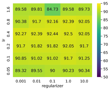
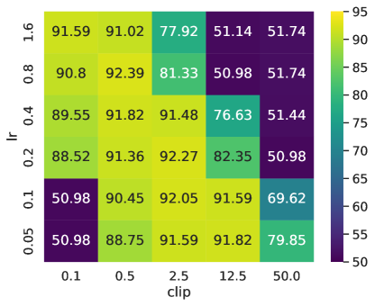
Figure 4: Experiments of fine-tuning RoBERTa on SST-2 task. Left: Accuracy heatmap of DP-NSGD with varying learning rates and regularizers. Right: Accuracy heatmap of DP-SGD with varying learning rates and clipping thresholds.

We have similar observation in Figure 4 that the performance of DP-NSGD is rather stable for the regularizer and the learning rate, which indicates that it could be easier to tune than DP-SGD.

We also run the experiments with DP-Adam and DP-NAdam optimizers. DP-Adam optimizer adds the per-example gradient clipping and Gaussian noise addition steps to Adam [26]. For DP-Adam, we search the clipping threshold $c$ takes values $\{0.1,0.5,2.5,12.5,50.0\}$ and the learning rate $lr$ taking values $\{\text{1e-4, 5e-4, 1e-3, 2e-3, 5e-3}\}$. For DP-NAdam, we use per-sample gradient normalization to replace the per-sample gradient clipping. We search the learning rate $lr$ from $\{\text{1e-4, 5e-4, 1e-3, 2e-3, 5e-3}\}$ and the regularizer factor $r$ from $\{\text{1e-3, 1e-2, 1e-1, 1., 10.0}\}$.

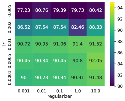
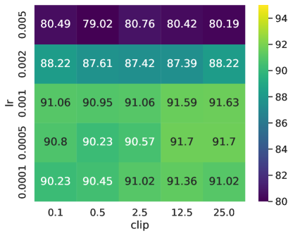
Figure 5: Left: Accuracy heatmap of DP-NAdam with varying learning rates and regularizers. Right: Accuracy heatmap of DP-Adam with varying learning rates and clips.

Appendix E Proof for Privacy Guarantee

This section presents a simple proof for Lemma 3.1. To begin with, we formally introduce the functional view of Renyi Differential Privacy below. Define a functional as

$$\epsilon_{\mathcal{M}}(\alpha)\triangleq\sup_{\mathbb{D},\mathbb{D}^{\prime}}D_{\alpha}(\mathcal{M}(\mathbb{D})\|\mathcal{M}(\mathbb{D}^{\prime}))=\sup_{\mathbb{D},\mathbb{D}^{\prime}}\frac{1}{\alpha-1}\log\mathbb{E}_{\theta\sim\mathcal{M}(\mathbb{D}^{\prime})}\left[\left(\frac{\mathcal{M}(\mathbb{D})(\theta)}{\mathcal{M}(\mathbb{D}^{\prime})(\theta)}\right)^{\alpha}\right],\alpha\geq 1$$ (45)

where $\mathcal{M}(\mathbb{D})$ denotes the distribution of the output with input $\mathbb{D}$ and $\mathcal{M}(\mathbb{D})(\theta)$ refers to the density at $\theta$ of this distribution. The following propositions clarify several notions of differential privacy in the literature.

Proposition E.1.

Let $\mathcal{M}$ be a randomized mechanism.

(i)

If and only if $\epsilon_{\mathcal{M}}(\infty)\leq\epsilon$, then $\mathcal{M}$ is $\epsilon$-(pure)-DP, [19].

(ii)

If and only if $\epsilon_{\mathcal{M}}(\alpha)\leq\epsilon$, then $\mathcal{M}$ is $(\alpha,\epsilon)$-RDP (Renyi differential privacy), [30].

(iii)

If and only if $\delta\geq\exp[(\alpha-1)(\epsilon_{\mathcal{M}}(\alpha)-\epsilon)]$ for some $\alpha\geq 1$, then $\mathcal{M}$ is $(\epsilon,\delta)$-DP, [20].

(iv)

If and only if $\epsilon_{\mathcal{M}}(\alpha)\leq\rho\alpha$ for any $\alpha\geq 1$, then $\mathcal{M}$ is $\rho$-zCDP (zero-concentrated differential privacy), [9].

(v)

If and only if $\epsilon_{\mathcal{M}}(\alpha)\leq\rho\alpha$ for any $\alpha\in(1,\omega)$, then $\mathcal{M}$ is $(\rho,\omega)$-tCDP (truncated concentrated differential privacy), [8].

We remark that Proposition E.1(iii) is adapted from the second assertion of Theorem 2 in [1], while the literature prefers to use the converse argument for this assertion, Proposition 3 in [30]. Here we also restate the composition theorem for Renyi differential privacy.

Proposition E.2 (Proposition 1, [30]).

Let $\mathcal{M}=\mathcal{M}_{T}\circ\mathcal{M}_{T-1}\circ\cdots\circ\mathcal{M}_{1}$ be defined in an interactively compositional way, then for any fixed $\alpha\geq 1$,

$$\epsilon_{\mathcal{M}}(\alpha)\leq\sum_{i=1}^{T}\epsilon_{\mathcal{M}_{i}}(\alpha).$$

DP-SGD and DP-NSGD under our consideration can both be decomposed into $T$ composition of sub-sampled Gaussian mechanism with uniform sampling without replacement, denoted as $\texttt{Gaussian}(\sigma)\circ\texttt{subsample}(N,B)$. We write the privacy-accountant functional, (45), of this building-block mechanism as $\hat{\epsilon}(\alpha)$.

It is widely known that the sole Gaussian mechanism has $\epsilon_{\texttt{Gaussian}(\sigma)}(\alpha)=\alpha/(2\sigma^{2})$, Table II in [30]. The sub-sampled Gaussian mechanism is much more complicated and draws many previous efforts. In particular, [1, 31] study Poisson sub-sampling, which is less popular in practical sub-sampling; [43] proposed a general bound for any uniformly sub-sampled RDP mechanisms, but their bound is a bit loose when restricted to Gaussian mechanisms. Thankfully, [8] developed a general privacy-amplification bound for any uniformly sub-sampled tCDP mechanisms, which is satisfying for our later treatment. Specifically, we specify Theorem 11 in [8] to the Gaussian mechanism, to get the following proposition.

Proposition E.3 (Privacy Amplification by Uniform Sub-sampling without Replacement).

For the very mechanism $\texttt{Gaussian}(\sigma)\circ\texttt{subsample}(N,B)$ with $B<0.1N$, we have the following privacy accountant

$$\hat{\epsilon}(\alpha)\leq\frac{7\gamma^{2}\alpha}{\sigma^{2}},\quad\forall\alpha\leq\frac{\sigma^{2}}{2}\log\left(\frac{1}{\gamma}\right),$$ (46)

with $\gamma=B/N$.

Proof of Lemma 3.1.

We denote whole composited mechanism as $\mathcal{M}$. By Propositions E.2 and E.3, we have

$$\epsilon_{\mathcal{M}}(\alpha)\leq\frac{7T\gamma^{2}\alpha}{\sigma^{2}},\quad\forall\alpha\leq\frac{\sigma^{2}}{2}\log\left(\frac{1}{\gamma}\right).$$

Further by Proposition E.1(iii), DP-SGD is $(\epsilon,\delta)$-DP if there exists $\alpha\leq\frac{\sigma^{2}}{2}\log\left(\frac{1}{\gamma}\right)$ such that

$$7T\gamma^{2}\alpha/\sigma^{2}\leq \epsilon/2,$$

$$\exp(-(\alpha-1)\epsilon/2)\leq \delta.$$

Plus, we find that when $\epsilon=c_{1}\gamma^{2}T$, we can satisfy all these conditions by setting

$$\sigma\geq c_{2}\frac{\gamma\sqrt{T\log(1/\delta)}}{\epsilon}$$

for some explicit constants $c_{1}$ and $c_{2}$. ∎

References

• [1] Martin Abadi, Andy Chu, Ian Goodfellow, Hย Brendan McMahan, Ilya Mironov, Kunal Talwar, and Liย Zhang. Deep learning with differential privacy. In ACM SIGSAC Conference on Computer and Communications Security, 2016.
• [2] Galen Andrew, Omย Thakkar, Hย Brendan McMahan, and Swaroop Ramaswamy. Differentially private learning with adaptive clipping. arXiv preprint arXiv:1905.03871, 2019.
• [3] Yossi Arjevani, Yair Carmon, Johnย C Duchi, Dylanย J Foster, Nathan Srebro, and Blake Woodworth. Lower bounds for non-convex stochastic optimization. arXiv preprint arXiv:1912.02365, 2019.
• [4] Hilal Asi, Johnย C. Duchi, Alireza Fallah, Omid Javidbakht, and Kunal Talwar. Private adaptive gradient methods for convex optimization. In Marina Meila and Tong Zhang, editors, Proceedings of the 38th International Conference on Machine Learning, ICML 2021, 18-24 July 2021, Virtual Event, volume 139 of Proceedings of Machine Learning Research, pages 383โ€“392. PMLR, 2021.
• [5] Raef Bassily, Adam Smith, and Abhradeep Thakurta. Differentially private empirical risk minimization: Efficient algorithms and tight error bounds. Annual Symposium on Foundations of Computer Science, 2014.
• [6] Zhiqi Bu, Jinshuo Dong, Qiย Long, and Weijieย J Su. Deep learning with gaussian differential privacy. Harvard data science review, 2020(23), 2020.
• [7] Zhiqi Bu, Hua Wang, Qiย Long, and Weijieย J Su. On the convergence of deep learning with differential privacy. arXiv preprint arXiv:2106.07830, 2021.
• [8] Mark Bun, Cynthia Dwork, Guyย N Rothblum, and Thomas Steinke. Composable and versatile privacy via truncated cdp. In Proceedings of the 50th Annual ACM SIGACT Symposium on Theory of Computing, 2018.
• [9] Mark Bun and Thomas Steinke. Concentrated differential privacy: Simplifications, extensions, and lower bounds. In Theory of Cryptography Conference, 2016.
• [10] Nicholas Carlini, Florian Tramer, Eric Wallace, Matthew Jagielski, Ariel Herbert-Voss, Katherine Lee, Adam Roberts, Tom Brown, Dawn Song, Ulfar Erlingsson, etย al. Extracting training data from large language models. arXiv preprint arXiv:2012.07805, 2020.
• [11] Kamalika Chaudhuri, Claire Monteleoni, and Anandย D Sarwate. Differentially private empirical risk minimization. Journal of Machine Learning Research, 2011.
• [12] Xiangyi Chen, Stevenย Z Wu, and Mingyi Hong. Understanding gradient clipping in private sgd: A geometric perspective. Advances in Neural Information Processing Systems, 33, 2020.
• [13] Ashok Cutkosky and Harsh Mehta. Momentum improves normalized sgd. In International Conference on Machine Learning, pages 2260โ€“2268. PMLR, 2020.
• [14] Ashok Cutkosky and Harsh Mehta. High-probability bounds for non-convex stochastic optimization with heavy tails. Advances in Neural Information Processing Systems, 34, 2021.
• [15] Rudrajit Das, Abolfazl Hashemi, Sujay Sanghavi, and Inderjitย S Dhillon. Dp-normfedavg: Normalizing client updates for privacy-preserving federated learning. arXiv preprint arXiv:2106.07094, 2021.
• [16] John Duchi, Elad Hazan, and Yoram Singer. Adaptive subgradient methods for online learning and stochastic optimization. Journal of machine learning research, 12(7), 2011.
• [17] Cynthia Dwork, Krishnaram Kenthapadi, Frank McSherry, Ilya Mironov, and Moni Naor. Our data, ourselves: Privacy via distributed noise generation. In Annual International Conference on the Theory and Applications of Cryptographic Techniques, 2006.
• [18] Cynthia Dwork, Frank McSherry, Kobbi Nissim, and Adam Smith. Calibrating noise to sensitivity in private data analysis. In Theory of cryptography conference, 2006.
• [19] Cynthia Dwork, Aaron Roth, etย al. The algorithmic foundations of differential privacy. Foundations and Trends in Theoretical Computer Science, 9(3-4):211โ€“407, 2014.
• [20] Cynthia Dwork, Kunal Talwar, Abhradeep Thakurta, and Liย Zhang. Analyze gauss: optimal bounds for privacy-preserving principal component analysis. In Proceedings of the forty-sixth annual ACM symposium on Theory of computing, 2014.
• [21] Saeed Ghadimi and Guanghui Lan. Stochastic first-and zeroth-order methods for nonconvex stochastic programming. SIAM Journal on Optimization, 23(4):2341โ€“2368, 2013.
• [22] Sivakanth Gopi, Yinย Tat Lee, and Lukas Wutschitz. Numerical composition of differential privacy. arXiv preprint arXiv:2106.02848, 2021.
• [23] Kaiming He, Xiangyu Zhang, Shaoqing Ren, and Jian Sun. Deep residual learning for image recognition. In Proceedings of the IEEE conference on computer vision and pattern recognition, 2016.
• [24] Geoffrey Hinton, Nitish Srivastava, and Kevin Swersky. Neural networks for machine learning lecture 6a overview of mini-batch gradient descent. Cited on, 14(8):2, 2012.
• [25] Jikai Jin, Bohang Zhang, Haiyang Wang, and Liwei Wang. Non-convex distributionally robust optimization: Non-asymptotic analysis. CoRR, abs/2110.12459, 2021.
• [26] Diederikย P Kingma and Jimmy Ba. Adam: A method for stochastic optimization. arXiv preprint arXiv:1412.6980, 2014.
• [27] Nurdan Kuru, ลžย ฤฐlker Birbil, Mert Gurbuzbalaban, and Sinan Yildirim. Differentially private accelerated optimization algorithms. arXiv preprint arXiv:2008.01989, 2020.
• [28] Xuechen Li, Florian Tramer, Percy Liang, and Tatsunori Hashimoto. Large language models can be strong differentially private learners. arXiv preprint arXiv:2110.05679, 2021.
• [29] Yinhan Liu, Myle Ott, Naman Goyal, Jingfei Du, Mandar Joshi, Danqi Chen, Omer Levy, Mike Lewis, Luke Zettlemoyer, and Veselin Stoyanov. Roberta: A robustly optimized bert pretraining approach. arXiv preprint arXiv:1907.11692, 2019.
• [30] Ilya Mironov. Rรฉnyi differential privacy. In IEEE Computer Security Foundations Symposium, 2017.
• [31] Ilya Mironov, Kunal Talwar, and Liย Zhang. Rรฉnyi differential privacy of the sampled gaussian mechanism. arXiv, 2019.
• [32] Shubhankar Mohapatra, Sajin Sasy, Xiย He, Gautam Kamath, and Omย Thakkar. The role of adaptive optimizers for honest private hyperparameter selection. arXiv preprint arXiv:2111.04906, 2021.
• [33] Nicolas Papernot, Steve Chien, Shuang Song, Abhradeep Thakurta, and Ulfar Erlingsson. Making the shoe fit: Architectures, initializations, and tuning for learning with privacy, 2020.
• [34] Nicolas Papernot and Thomas Steinke. Hyperparameter tuning with renyi differential privacy. arXiv preprint arXiv:2110.03620, 2021.
• [35] Nicolas Papernot, Abhradeep Thakurta, Shuang Song, Steve Chien, and รšlfar Erlingsson. Tempered sigmoid activations for deep learning with differential privacy. arXiv preprint arXiv:2007.14191, 2020.
• [36] Venkatadheeraj Pichapati, Anandaย Theertha Suresh, Felixย X Yu, Sashankย J Reddi, and Sanjiv Kumar. Adaclip: Adaptive clipping for private sgd. arXiv preprint arXiv:1908.07643, 2019.
• [37] Karthikย Abinav Sankararaman, Soham De, Zheng Xu, Wย Ronny Huang, and Tom Goldstein. The impact of neural network overparameterization on gradient confusion and stochastic gradient descent. In International Conference on Machine Learning, pages 8469โ€“8479. PMLR, 2020.
• [38] Florian Tramรจr and Dan Boneh. Differentially private learning needs better features (or much more data). arXiv preprint arXiv:2011.11660, 2020.
• [39] Alex Wang, Amanpreet Singh, Julian Michael, Felix Hill, Omer Levy, and Samuelย R Bowman. Glue: A multi-task benchmark and analysis platform for natural language understanding. arXiv preprint arXiv:1804.07461, 2018.
• [40] Diย Wang, Changyou Chen, and Jinhui Xu. Differentially private empirical risk minimization with non-convex loss functions. In International Conference on Machine Learning, pages 6526โ€“6535. PMLR, 2019.
• [41] Diย Wang, Minwei Ye, and Jinhui Xu. Differentially private empirical risk minimization revisited: Faster and more general. In Advances in Neural Information Processing Systems, 2017.
• [42] Puyu Wang, Yunwen Lei, Yiming Ying, and Hai Zhang. Differentially private sgd with non-smooth losses. Applied and Computational Harmonic Analysis, 56:306โ€“336, 2022.
• [43] Yu-Xiang Wang, Borja Balle, and Shivaย Prasad Kasiviswanathan. Subsampled rรฉnyi differential privacy and analytical moments accountant. In International Conference on Artificial Intelligence and Statistics, 2019.
• [44] Yuxin Wu and Kaiming He. Group normalization. In Proceedings of the European conference on computer vision (ECCV), 2018.
• [45] Yang You, Jing Li, Jonathan Hseu, Xiaodan Song, James Demmel, and Cho-Jui Hsieh. Reducing BERT pre-training time from 3 days to 76 minutes. CoRR, abs/1904.00962, 2019.
• [46] Daย Yu, Huishuai Zhang, Wei Chen, Jian Yin, and Tie-Yan Liu. Gradient perturbation is underrated for differentially private convex optimization. In Proc. of 29th Int. Joint Conf. Artificial Intelligence, 2020.
• [47] Bohang Zhang, Jikai Jin, Cong Fang, and Liwei Wang. Improved analysis of clipping algorithms for non-convex optimization. In Hugo Larochelle, Marcโ€™Aurelio Ranzato, Raia Hadsell, Maria-Florina Balcan, and Hsuan-Tien Lin, editors, Advances in Neural Information Processing Systems (NeurIPS), 2020.
• [48] Jingzhao Zhang, Tianxing He, Suvrit Sra, and Ali Jadbabaie. Why gradient clipping accelerates training: A theoretical justification for adaptivity. In International Conference on Learning Representations (ICLR), 2020.
• [49] Xinwei Zhang, Xiangyi Chen, Mingyi Hong, Zhiweiย Steven Wu, and Jinfeng Yi. Understanding clipping for federated learning: Convergence and client-level differential privacy. arXiv preprint arXiv:2106.13673, 2021.
• [50] Shen-Yi Zhao, Yin-Peng Xie, and Wu-Jun Li. On the convergence and improvement of stochastic normalized gradient descent. Science China Information Sciences, 64(3):1โ€“13, 2021.