Quantum diffusion via an approximate semigroup property

Abstract.

In this paper we introduce a new approach to the diffusive limit of the weakly random Schrodinger equation, first studied by L. Erdos, M. Salmhofer, and H.T. Yau. Our approach is based on a wavepacket decomposition of the evolution operator, which allows us to interpret the Duhamel series as an integral over piecewise linear paths. We relate the geometry of these paths to combinatorial features of a diagrammatic expansion which allows us to express the error terms in the expansion as an integral over paths that are exceptional in some way. These error terms are bounded using geometric arguments. The main term is then shown to have a semigroup property, which allows us to iteratively increase the timescale of validity of an effective diffusion. This is the first derivation of an effective diffusion equation from the random Schrodinger equation that is valid in dimensions $d\geq 2$.

1. Introduction

1.1. The kinetic limit for the Schödinger equation

In this paper, we study the equation

(1.1) $$i\partial_{t}\psi=-\frac{1}{2}\Delta\psi+{\varepsilon}V\psi$$

with a stationary random potential $V$. An example of a potential we will consider is a mean- zero Gaussian random field with a smooth and compactly supported two point correlation function

(1.2) $${\mathbf{E}\,}V(x)V(y)=R(x-y).$$

with $R\in C_{c}^{\infty}({\mathbf{R}}^{d})$. Our approach works for more general potentials that are stationary, have finite range of dependence, and have bounded moments in $C^{k}$ (for $k>20d$, say).

The equation (1.1) is a simple model for wave propagation in a random environment. It also has a more direct physical significance, as it models the motion of a cold electron in a disordered environment [29]. We are interested in this paper in the regime where the frequency of the initial condition $\psi$ is comparable to the correlation length of the potential, which we consider to be of unit scale. This regime is out of reach of both traditional WKB-type semiclassical approximations, which are more appropriate for high-frequency $\psi$, and of homogenization techniques, which are appropriate for low-frequency $\psi$.

This regime was first rigorously studied by H. Spohn in [29] , who showed that the spectral density $\mu_{t}(p)={\mathbf{E}\,}|\psi_{t/{\varepsilon}^{2}}(p)|^{2}$ converges, in the semiclassical limit ${\varepsilon}\to 0$, to a weak solution of a spatially homogeneous kinetic equation

(1.3) $$\partial_{t}\mu(p)=\int\delta(|p|^{2}-|p^{\prime}|^{2}){\widehat{R}}(p-p^{\prime})[\mu(p^{\prime})-\mu(p)]\mathop{}\!\mathrm{d}p^{\prime},$$

where $R(x)$ is the two-point correlation function defined in (1.2). The term $\delta(|p|^{2}-|p^{\prime}|^{2})$ enforces conservation of kinetic energy, which is appropriate in the limit ${\varepsilon}\to 0$ since the potential energy becomes negligible. The time scale between scattering events is on the order ${\varepsilon}^{-2}$, which can be heuristically justified by using the Born approximation of the solution of (1.1). Spohn’s technique for demonstrating (1.3) was to write out the Duhamel expansion for the solution $\psi_{t}(p)$ to (1.1) in momentum space, take an expectation of the quantity $|\psi_{t}(p)|^{2}$ using the Wick rule for the expectation of a product of Gaussian random variables, and separate terms into a main term and an error term. The error terms are controlled by additional cancellations and the main terms are compared to a series expansion for the solution of (1.3). Spohn’s analysis of the Dyson series allowed him to control the solution up to times $c{\varepsilon}^{-2}$ for some small constant $c>0$.

This proof technique has been used by many authors since to improve upon our understanding of (1.1). Most notably, L. Erdös and H.T. Yau in a series of works [17, 18] were able to improve the time scale to arbitrary kinetic times of the form of the order $O({\varepsilon}^{-2})$ while also demonstrating the weak convergence of the Wigner function

$${\mathcal{W}_{\psi}}(x,p):=\int e^{iy\cdot p}\overline{\psi}(x-y/2)\psi(x+y/2)\mathop{}\!\mathrm{d}y$$

to the solution of the linear Boltzmann equation

(1.4) $$\partial_{t}\rho+p\cdot\nabla_{x}\rho={\varepsilon}^{2}\int\delta(|p|^{2}-|p^{\prime}|^{2}){\widehat{R}}(p-p^{\prime})[\rho(x,p^{\prime})-\rho(x,p)]\mathop{}\!\mathrm{d}p^{\prime}.$$

Introducing the rescaled coordinates $T={\varepsilon}^{2}t$, $X={\varepsilon}^{2}x$ along with the rescaled solution

$$\rho^{\varepsilon}_{T}(X,p):=\rho_{{\varepsilon}^{-2}T}({\varepsilon}^{-2}x,p),$$

the equation (1.4) can be written

$$\partial_{T}\rho^{\varepsilon}+p\cdot\nabla_{X}\rho=\int\delta(|p|^{2}-|p^{\prime}|^{2}){\widehat{R}}(p-p^{\prime})[\rho^{\varepsilon}(X,p^{\prime})-\rho^{\varepsilon}(X,p)]\mathop{}\!\mathrm{d}p^{\prime}.$$

In an impressive sequence of refinements to this work, L. Erdos, M. Salmhofer and H.T. Yau [14, 16, 15] were able to improve the timescale even further to diffusive times ${\varepsilon}^{-2-\kappa}$ for some positive $\kappa>0$ (in fact, one can take $\kappa=1/370$ when $d=3$). At this timescale a diffusion equation emerges. The principle is that the momentum variable is no longer relevant to the evolution because it becomes uniformly distributed over the sphere within time $O({\varepsilon}^{-2})$, and all that remains of the momentum information is the kinetic energy variable $e=|p|^{2}/2$. Moreover, for diffusive times ${\varepsilon}^{-2-\kappa}$ the particle travels a distance ${\varepsilon}^{-2-\kappa/2}$ so the diffusive length scale is ${\varepsilon}^{-2-\kappa/2}$.

For solutions $\rho$ of the linear Boltzmann equation (1.4), the particle distribution $f$ defined by

(1.5) $$f_{T}(X,e)=\int_{|p|^{2}/2=e}\rho_{{\varepsilon}^{-2-\kappa}T}({\varepsilon}^{-2-\kappa/2}X,p)\mathop{}\!\mathrm{d}{\mathcal{H}}^{n-1}(p)$$

converges in the limit ${\varepsilon}\to 0$ to a solution of the diffusion equation

(1.6) $$\partial_{T}f_{T}=D_{e}\Delta_{X}f_{T},$$

where $D_{e}$ is a diffusion coefficient depending on the energy $e$. See [16] for more details on the limiting diffusion equation.

To reach the diffusive time scale in which the particle experiences infinitely many scattering events, one must consider terms with ${\varepsilon}^{-c}$ collisions, which produces more than ${\varepsilon}^{-{\varepsilon}^{-c}}$ diagrams when one applies the Wick expansion. To deal with the explosion in the number of terms, Erdos, Salmhofer, and Yau developed a resummation technique to more accurately estimate the sizes of the terms and additionally had to exploit intricate cancellations coming from the combinatorial features of the diagrams considered.

1.2. Statement of the main result

In this paper, we provide an alternative derivation of the linear Boltzmann equation which is also valid up to diffusive times but with a fundamentally different approach. In our proof, we use a wavepacket decomposition of the evolution operator. The wavepacket decomposition allows us to keep information about the position and momentum of the particle simultaneously (up to the limits imposed by the uncertainty principle), and we therefore express the solution as an integral over piecewise linear paths in phase space.

To make the connection between operators and the linear Boltzmann equation, we use the Weyl quantization $a\in C^{\infty}({{\mathbf{R}}^{2d}})\mapsto\operatorname{Op}^{w}(a)\in\mathcal{B}(L^{2}({\mathbf{R}}^{d}))$ defined by

$$\operatorname{Op}^{w}(a)f(x)=\int e^{i(x-y)\cdot p}a((x+y)/2,p)f(y)\mathop{}\!\mathrm{d}y\mathop{}\!\mathrm{d}p.$$

The relationship between the Weyl quantization and the Wigner transform is given by the identity

$$\langle\operatorname{Op}^{w}(a)\psi,\psi\rangle=\int a(x,p){\mathcal{W}_{\psi}}(x,p)\mathop{}\!\mathrm{d}x\mathop{}\!\mathrm{d}p.$$

In particular, applying this identity to the solution $\psi_{t}=e^{-itH}\psi$ to (1.1) where $H$ is the random Hamiltonian

$$H=-\frac{1}{2}\Delta+{\varepsilon}V,$$

we have

$$\int a(x,p){\mathbf{E}\,}{\mathcal{W}_{\psi_{t}}}(x,p)\mathop{}\!\mathrm{d}x\mathop{}\!\mathrm{d}p={\mathbf{E}\,}\langle\operatorname{Op}^{w}(a)e^{-itH}\psi,e^{-itH}\psi\rangle=\langle{\mathbf{E}\,}e^{itH}\operatorname{Op}^{w}(a)e^{-itH}\psi,\psi\rangle.$$

Therefore in order to answer questions about the weak convergence of ${\mathcal{W}_{\psi_{t}}}$, it suffices to study the quantum evolution channel

(1.7) $${\mathcal{E}}_{t}[A]:={\mathbf{E}\,}e^{itH}Ae^{-itH}$$

applied to operators of the form $A=\operatorname{Op}^{w}(a)$ with sufficiently regular symbols $a$. In particular, we will show that for suitable observables $a_{0}$ and for times $t\leq{\varepsilon}^{-2-\kappa}$, we have

$$\|{\mathcal{E}}_{t}[\operatorname{Op}^{w}(a_{0})]-\operatorname{Op}^{w}(a_{t})\|_{op}=o(1),$$

where $a_{t}$ solves the dual of the linear Boltzmann equation (1.4),

(1.8) $$\partial_{t}a-p\cdot\nabla_{x}a={\varepsilon}^{2}\int\delta(|p|^{2}-|p^{\prime}|^{2}){\widehat{R}}(p-p^{\prime})[a(x,p^{\prime})-a(x,p)]\mathop{}\!\mathrm{d}p^{\prime}.$$

A natural norm that we use on $a$ which also controls the operator norm of $\operatorname{Op}^{w}(a)$ is the $C^{k}$ norm with $k=2d+1$ (see Appendix C for a self-contained proof that the $C^{2d+1}$ norm of $a$ controls the operator norm of $\operatorname{Op}^{w}(a)$). We will use a $C^{k}$ norm which is rescaled to the appropriate length scales of the problem. Because the time scale between scattering events is ${\varepsilon}^{-2}$, a natural spatial length scale is ${\varepsilon}^{-1}$. For the rest of the paper we write $r={\varepsilon}^{-1}$ for this length scale. This is the length scale of a wavepacket that remains coherent between scattering events. Conversely the natural length scale in momentum is ${\varepsilon}=r^{-1}$. This “microscopic” scale is the one we use for the wavepacket decomposition of the operator $e^{itH}$.

On the other hand, a natural “macroscopic” length scale of the problem is ${\varepsilon}^{-2}$, which is the distance that a particle with momentum $O(1)$ travels between scatterings. A natural “macroscopic” length scale in momentum is $O(1)$, which is the impulse applied to a particle in a typical scattering event.

The following norm measures the smoothness of an observable at these length scales:

$$\|a\|_{C^{k}_{r,L}}:=\sum_{|\alpha_{x}|+|\alpha_{p}|\leq k}\sup_{(x,p)}|(rL\partial_{x})^{\alpha_{x}}(r^{-1}L\partial_{p})^{\alpha_{p}}a(x,p)|.$$

When $L=1$, this norm probes the microscopic smoothness of observables, whereas when $L={\varepsilon}^{-1}$, the norm probes the macroscopic smoothness.

We make one final comment before we state the main result of the paper, which is that we will not treat the evolution of low-frequency modes. In dimension $d=2$, the scattering cross section of a low frequency wave with momentum $|p|\ll 1$ is still on the order ${\varepsilon}^{2}$ but the speed of travel is only $|p|$, so the distance between typical scattering events is only $|p|{\varepsilon}^{-2}$ rather than ${\varepsilon}^{-2}$. Because scattering events are more closely spaced, the bounds coming from the geometric arguments we use deteriorate and we make no attempt to understand what happens in this regime. In higher dimensions the scattering cross section also shrinks with momentum so that one could in principle first approximate the evolution of low frequency modes by a free evolution with no potential and therefore recover the result for all frequencies. We do not make this argument in this paper.

Theorem 1.1.

For each $d\geq 2$, there exists $\theta=\theta(d)>0$ and $\kappa=\kappa(d)>0$ such that the following holds. Let $V$ be an admissible potential as described in Definition (B.2), and let $a_{0}\in C^{2d+1}({{\mathbf{R}}^{2d}})$ be a classical observable supported away from zero momentum;

$$\operatorname{supp}a_{0}\subset\{(x,p)\in{{\mathbf{R}}^{2d}}\mid|p|\geq{\varepsilon}^{\theta(d)}\}.$$

Suppose moreover that $a_{t}$ solves (1.8) with initial condition $a_{0}$. Then

(1.9) $$\|{\mathcal{E}}_{t}[\operatorname{Op}^{w}(a_{0})]-\operatorname{Op}^{w}(a_{t})\|_{op}\leq C_{d}{\varepsilon}^{2+\kappa}t\|a_{0}\|_{C^{2d+1}_{{\varepsilon}^{-1},{\varepsilon}^{-0.5}}}.$$

In particular, for arbitrary $\psi_{0}\in L^{2}({\mathbf{R}}^{d})$ and $\psi_{t}$ solving (1.1) it follows that

(1.10) $$\int{\mathcal{W}_{\psi_{t}}}(x,p)a_{0}(x,p)\mathop{}\!\mathrm{d}x\mathop{}\!\mathrm{d}p=\int{\mathcal{W}_{\psi_{0}}}(x,p)a_{t}(x,p)\mathop{}\!\mathrm{d}x\mathop{}\!\mathrm{d}p+O({\varepsilon}^{2+\kappa}t\|a_{0}\|_{C^{2d+1}_{{\varepsilon}^{-1},{\varepsilon}^{-0.5}}}\|\psi\|_{L^{2}}^{2}).$$

To see how the diffusion equation (1.6) emerges as a scaling limit, we consider observables of the form

$$a_{0}(x,p)=\bar{a}({\varepsilon}^{2+\kappa/2}x,p)$$

with $\bar{a}\in C^{2d+1}$. With this rescaling, we have

$$\|a_{0}\|_{C^{2d+1}_{{\varepsilon}^{-1},{\varepsilon}^{-1}}}\leq\|\bar{a}\|_{C^{2d+1}}.$$

In particular, $\|a_{0}\|_{C^{2d+1}_{{\varepsilon}^{-1},{\varepsilon}^{-0.5}}}$ is bounded uniformly in ${\varepsilon}$. Moreover, the solution $a_{t}$ solves (1.6).

One major difference between Theorem 1.1 and the main results of [16, 15], apart from the very different approaches to the proof, is that our result holds in dimension $d=2$. At first this may appear to be in contradiction with the conjectured phenomenon of Anderson localization in $d=2$, but the contradiction disappears when one compares the timescale ${\varepsilon}^{-2-\kappa}$ considered in this paper to the expected length scale $e^{{\varepsilon}^{-2}}$ of localization in this dimension. Indeed, it is expected that the particle exhibits diffusive behavior for an exponentially long time before getting trapped by localization.

The exponent $\kappa(d)$ can in principle be extracted from the proof. However in this paper we focus on demonstrating the new technique in its simplest form and therefore do not attempt to optimize $\kappa(d)$. Perhaps with some optimization one could obtain $\kappa(3)$ comparable to $1/370$, but the proof we give yields a bound of the order $\kappa(3)\sim 10^{-6}$.

1.3. A heuristic sketch of the argument

1.3.1. The phase space path integral

The main idea behind the proof of Theorem 1.1 is to focus on justifying an approximate semigroup property

(1.11) $${\mathcal{E}}_{2t}[A]\approx{\mathcal{E}}_{t}[{\mathcal{E}}_{t}[A]],$$

for suitable operators $A$ including operators of the form $A=\operatorname{Op}^{w}(a)$. Observe that the approximation (1.11) has the following physical interpretation. Let

$$H_{1} =-\frac{1}{2}\Delta+{\varepsilon}V_{1}$$

$$H_{2} =-\frac{1}{2}\Delta+{\varepsilon}V_{2}.$$

be Hamiltonians with two independently sampled potentials, and observe that

$${\mathcal{E}}_{t}\circ{\mathcal{E}}_{t}[A]={\mathbf{E}\,}e^{itH_{2}}e^{itH_{1}}Ae^{-itH_{1}}e^{-itH_{2}}.$$

In other words, ${\mathcal{E}}_{t}\circ{\mathcal{E}}_{t}$ represents an evolution with a potential that abruptly changes into an independently sampled potential at time $t$. Although such a resampling of the potential drastically changes the evolution of the wavefunction $\psi_{t}$ itself, we will see that the effect on observables is minimal

To prove the approximate semigroup property we approximate the evolution operator $e^{-itH}$ as an integral over piecewise linear paths in phase space, representing the possible paths of a particle as it scatters. To decompose phase space we use a family of wavepackets of the form

$$\phi_{x,p}(y):=r^{-d/2}e^{iy\cdot p}\chi_{env}((x-y)/r),$$

where $\chi_{env}\in C_{c}^{\infty}({\mathbf{R}}^{d})$ is a fixed envelope normalized in $L^{2}$ and satisfying some additional conditions described in Appendix C. The functions $\phi_{x,p}$ are localized in space to scale $r$ and in momentum to scale $r^{-1}$. We use the notation $\xi=(x,p)$ and write $\mathinner{|{\xi}\rangle}$ as a shorthand for the function $\phi_{\xi}$.

The use of a phase-space path integral already represents a departure from previous approaches to the problem. Indeed, since the paper of Spohn [29] it has been customary to write the terms of the Duhamel series expansion for $e^{itH}$ in the Fourier basis. We will see that by using the spatial localization of the particle we can more easily compute the expectation appearing in the integrand without the need for a full Wick expansion (or cumulant decomposition in the case of a non-Gaussian potential).

The free evolution of a wavepacket approximates the motion of a free classical particle in the sense that

$$e^{-it\Delta/2}\mathinner{|{(x,p)}\rangle}\approx e^{it|p|^{2}/2}\mathinner{|{(x+tp,p)}\rangle}$$

for $t\ll r^{2}$. For multiplication against the potential we use the identity

(1.12) $$V\mathinner{|{(x,p)}\rangle}=\int{\widehat{V_{x}}}(p^{\prime}-p)\mathinner{|{(x,p^{\prime})}\rangle}\mathop{}\!\mathrm{d}p^{\prime},$$

where $V_{x}$ is the potential $V$ multiplied by a cutoff near $y$ which is $1$ in a ball large enough to contain the support of $\chi_{env}$,

$$V_{x}(y)=b((y-x)/r)V(y).$$

We can use these two identities to write an expansion of the evolution of a wavepacket $e^{itH}\mathinner{|{(x,p)}\rangle}$ as an integral over paths in which the phase space point travels in straight lines with an occasional impulse from the potential causing discontinuities in the momentum variable. We represent these piecewise linear paths as a tuple $\omega=({\mathbf{s}},{\mathbf{p}},{\mathbf{y}})$ with ${\mathbf{s}}=(s_{0},\cdots,s_{k})$ being the sequence of times between the scattering events (satisfying $\sum s_{j}=t$ and $s_{j}\geq 0$), ${\mathbf{p}}=(p_{0},p_{1}\cdots,p_{k})$ being the sequence of momentum variables which we require to have the same magnitude $|p_{j}|=|p_{j^{\prime}}|$ and with initial momentum $p_{0}=p$, and ${\mathbf{y}}=(y_{1},\cdots,y_{k})$ being the sequence of scattering locations defined by

$$y_{1} =x+s_{0}p$$

$$y_{j+1} =y_{j}+s_{j}p_{j}.$$

An example of a path is depicted in Figure 1.

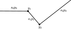
Figure 1. A sample scattering path of a particle with $2$ collisions. The displacement between consecutive collisions is given by $s_{j}p_{j}$, where $p_{j}\in{\mathbf{R}}^{d}$ is a momentum vector with constrained kinetic energy $|p_{j}|^{2}/2$, and $s_{j}\geq 0$ is the time between collisions.

Each such path $\omega$ defines an operator $O_{\omega}$ which approximately acts on wavepackets by

(1.13) $$O_{\omega}\mathinner{|{(x,p)}\rangle}=e^{i\varphi(\omega)}\prod_{j=1}^{k}{\widehat{V_{y_{j}}}}(p_{j}-p_{j-1})\mathinner{|{y_{k}+s_{k}p_{k},p_{k}}\rangle},$$

where $\varphi(\omega)$ is a deterministic phase accumulated from the stretches of free evolution. These phases do not matter for this sketch of the proof. However, in the actual proof we use stationary phase to ensure that the geometric constraints $y_{j+1}=y_{j}+s_{j}p_{j}$ are approximately satisfied and to show that kinetic energy is approximately conserved. Then, at least formally, we can write out the path integral for the evolution of a wavepacket $\mathinner{|{\xi}\rangle}$ as

(1.14) $$e^{itH}\mathinner{|{\xi}\rangle}=\int O_{\omega}\mathinner{|{\xi}\rangle}\mathop{}\!\mathrm{d}\omega.$$

We apply this decomposition of the evolution to investigate the approximate semigroup property for operators of the form

$$A=\int_{{{\mathbf{R}}^{2d}}}a(\xi)\mathinner{|{\xi}\rangle}\mathinner{\langle{\xi}|}\mathop{}\!\mathrm{d}\xi,$$

which are local in phase space in the sense that

$$A\mathinner{|{\xi}\rangle}\approx a(\xi)\mathinner{|{\xi}\rangle}.$$

Using the path integral (1.14) in the definition of ${\mathcal{E}}_{t}[A]$ we obtain

$${\mathcal{E}}_{t}[A]=\int_{{{\mathbf{R}}^{2d}}}\iint{\mathbf{E}\,}O_{\omega^{\prime}}^{*}\mathinner{|{\xi}\rangle}\mathinner{\langle{\xi}|}O_{\omega}\mathop{}\!\mathrm{d}\omega\mathop{}\!\mathrm{d}\omega^{\prime}\mathop{}\!\mathrm{d}\xi.$$

What is important for this sketch of the proof is to simply investigate which pairs of paths $\omega$ and $\omega^{\prime}$ have

$${\mathbf{E}\,}O_{\omega^{\prime}}^{*}\mathinner{|{\xi}\rangle}\mathinner{\langle{\xi}|}O_{\omega}\not=0.$$

In particular, we are interested in understanding for which sequence of positions $y_{j},y^{\prime}_{j}$ and impulses $q_{j},q^{\prime}_{j}$ we have

$${\mathbf{E}\,}\prod_{j=1}^{k}{\widehat{V_{y_{j}}}}(q_{j})\prod_{j^{\prime}=1}^{k^{\prime}}{\widehat{V_{y^{\prime}_{j^{\prime}}}}}^{*}(q^{\prime}_{j^{\prime}})\not=0.$$

Using the fact that $V$ is real and therefore ${\widehat{V_{y}}}^{*}(q)={\widehat{V_{y}}}(-q)$, we can rewrite the expectation above as

$${\mathbf{E}\,}\prod_{b\in[k]\sqcup[k^{\prime}]}{\widehat{V_{y_{b}}}}(q_{b}),$$

where $[k]\sqcup[k^{\prime}]$ is shorthand for the doubled index set $[k]\times\{0\}\cup[k^{\prime}]\times\{1\}$ and the $q_{b}$ impulses are reversed for $b=(j,1)$, so in particular $q_{j,1}=-(p^{\prime}_{j}-p^{\prime}_{j-1})$. Because $V_{y}$ are localized, the expectation above splits along a partition $P({\mathbf{y}},{\mathbf{y}}^{\prime})\in{\mathcal{P}}([k]\sqcup[k^{\prime}])$ defined by the clusters of the collision locations $y_{b}$ (so that $b\sim_{P}b^{\prime}$ when $|y_{b}-y_{b^{\prime}}|{\,\lesssim\,}r$). That is, we have an identity of the form

$${\mathbf{E}\,}\prod_{b\in[k]\sqcup[k^{\prime}]}{\widehat{V_{y_{b}}}}(q_{b})=\prod_{S\in P({\mathbf{y}},{\mathbf{y}}^{\prime})}{\mathbf{E}\,}\prod_{b\in S}{\widehat{V_{y_{b}}}}(q_{b}).$$

Within each cluster the expectations is zero unless the sum of the impulses is zero. This “conservation of momentum” condition is a consequence of the stationarity of the potential and is made rigorous in Lemma B.3. In the case of Gaussian potentials, this is a consequence of the Wick formula and the identity

$${\mathbf{E}\,}{\widehat{V}}(p){\widehat{V}}(q)={\widehat{R}}(p)\delta(p+q).$$

We are led to the following purely geometric constraints on the pair of paths $\omega,\omega^{\prime}$.

Definition 1.2.

Two paths $\omega,\omega^{\prime}$ are said to be compatible if the partition $P({\mathbf{y}},{\mathbf{y^{\prime}}})$ has no singletons and

$$\sum_{b\in S}q_{b}=0$$

for every $S\in P({\mathbf{y}},{\mathbf{y^{\prime}}})$.

1.3.2. Geometric characterization of the error term

This geometric notion of compatible paths is perhaps the most significant idea in the proof. Indeed, the point is that we can usefully manipulate the path integral before computing an expectation. In other words, we will first decompose the path integral according to geometry and then allow the geometry to dictate the combinatorics of the diagrams.

Now, we take a step back to appreciate which paths contribute to the error term in the semigroup property. As the discussion above indicates, the semigroup property compares the evolution ${\mathcal{E}}_{t}$ with a fixed potential $V$ to the evolution ${\mathcal{E}}_{t/2}\circ{\mathcal{E}}_{t/2}$ during which the potential is refreshed from $V_{1}$ to $V_{2}$ at time $t/2$. To keep track of which potential a scattering event sees we introduce the collision times $t_{b}$, defined by $t_{0}=0$ and $t_{b+1}=t_{b}+s_{b}$. The following condition suffices to ensure that the pair of paths $(\omega,\omega^{\prime})$ has an expected amplitude that is unaffected by the possibility of a time-dependent potential.

Definition 1.3.

Two paths $\omega,\omega^{\prime}$ are time-consistent if $t_{b}=t_{b^{\prime}}$ for all pairs of indices $b,b^{\prime}\in[k]\sqcup[k^{\prime}]$ such that $y_{b}=y_{b^{\prime}}$. Pairs $(\omega,\omega^{\prime})$ that are not time-consistent are said to be time-inconsistent.

Observe that $\omega$ is compatible with itself and is also time-consistent. We will show that in fact the paths $(\omega,\omega^{\prime})$ in which $\omega=\omega^{\prime}$ or is otherwise a small perturbation of $\omega$ form the bulk of the contribution to ${\mathcal{E}}_{t}$.

To understand the error term, we characterize pairs of paths $(\omega,\omega^{\prime})$ which are compatible but time-inconsistent. A simple way that a pair $(\omega,\omega^{\prime})$ could be time-inconsistent is if either $\omega$ or $\omega^{\prime}$ have a recollision. A simple example of a pair of compatible paths which are time-inconsistent due to a recollision is depicted in Figure 2

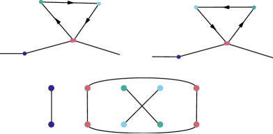
Figure 2. An example of a pair of paths with a recollision. The paths $\omega$ and $\omega^{\prime}$ are depicted at the top left and top right, and the collisions are colored according to the cluster in the partition $P(\omega,\omega^{\prime})$. On the bottom, an abstract depiction of the partition $P(\omega,\omega^{\prime})$. Notice that there is a red cluster with $4$ collisions, two from $\omega$ and two from $\omega^{\prime}$.

There is another geometric feature which we call a “tube event” which occurs when three collisions are collinear (in general, when they lie on narrow tube). Tube events can also lead to time inconsistencies, as depicted in Figure 3

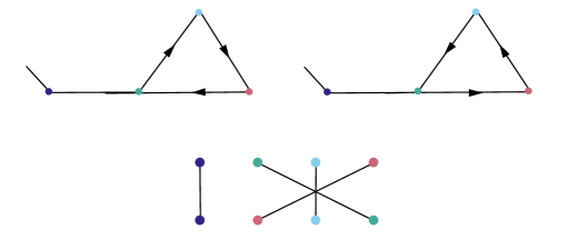
Figure 3. An example of a tube event. Note that there are three collisions lying on a line, but neither $\omega$ nor $\omega^{\prime}$ forms a recollision. Nonetheless, the collisions are time-inconsistent because the second collision of $\omega$ coincides with the fourth collision of $\omega^{\prime}$, as shown in the diagram of $P(\omega,\omega^{\prime})$ below.

We note that the estimation of the contribution of these special geometric features replaces the need for crossing estimates such as the ones studied in [23]. Our diagrams are bounded using relatively simple-minded volumetric considerations (essentially, after taking care of deterministic cancellations in the integral, we use the triangle inequality and account for the contribution of each degree of freedom). This simple-minded approach works particularly well for subkinetic timescales $\tau{\,\lesssim\,}{\varepsilon}^{-2+\kappa/2}$ in which one only needs $k_{max}=O(\kappa^{-1})$ collisions in the series expansion to approximate $e^{i\tau H}$ and therefore all combinatorial factors are bounded by a (very large) absolute constant.

The general strategy of the proof therefore is as follows:

1. Classify the geometric behaviors that can lead to time-inconsistencies.

2. Partition the path integral into paths with bad behaviors and paths without bad behaviors.

3. Use geometric estimates to bound the operator norm of the contribution of the bad paths.

The main new feature of this proof strategy is that the path integral is partitioned before the expectation is computed. That is, we do not decompose the expectation until we already have some information about the partition $P(\omega,\omega^{\prime})$. This is in contrast to the traditional approach used in [29, 16, 15, 18] which is summarized below.

1. Expand the expectation using the Wick rule or a cumulant expansion.

2. Partition the diagrams according to complexity by a combinatorial criterion.

3. Use oscillatory integral estimates to bound the contributions of the bad diagrams.

1.3.3. Reaching the diffusive timescale

To reach the diffusive timescale we prove a semigroup property of the form

$${\mathcal{E}}_{N\tau}\approx{\mathcal{E}}_{\tau}^{N}$$

where $\tau={\varepsilon}^{-2+\kappa/2}$ and $N={\varepsilon}^{-\kappa}$. The challenge we face in trying to understand the evolution operator $e^{itH}$ for times $t\sim{\varepsilon}^{-2-\delta}$ is that one needs to resolve at least ${\varepsilon}^{-\delta}$ collisions. This requires a path integral in a space of dimension ${\varepsilon}^{-\delta}$. If we then try to use crude estimates to bound the contribution of the terms in the Duhamel expansion we may lose a factor of $C^{{\varepsilon}^{-\delta}}$. What we need to do is take into account cancellations that occur between the terms in the Duhamel expansion. In [16, 15] this is done by renormalizing the propagator. This is equivalent to viewing $H=-\Delta/2+{\varepsilon}V$ not as a perturbation of the free evolution $-\Delta/2$ but as a perturbation of $-\Delta/2+{\varepsilon}^{2}\Theta$ where $\Theta$ is a multiplier operator that takes into account the effect of immediate recollisions. The multiplier $\Theta$ has a nonzero imaginary part so that $e^{-i\Delta/2+i\Theta}$ decays exponentially in time. This exponential decay exactly matches the exponential growth in the volume of the path inetgral. The value of $\Theta$ is also chosen so that a precise cancellation occurs in diagrams with immediate recollisions.

We take an alternative approach to resummation. The idea is that we first write

$$e^{itH}=e^{iN\tau H}=e^{i\tau H}\cdots e^{i\tau H},$$

where $N\sim{\varepsilon}^{-\kappa}$ and $\tau\sim{\varepsilon}^{-2+\kappa/2}$. Each of the terms $e^{i\tau H}$ is expanded as a Duhamel series of $k_{max}$ terms. We then partition the resulting path integral into pieces depending on geometric features of the paths and decompose the expectation using this geometric information. When this is done we resum the terms in the Duhamel series corresponding to segments that do not have any geometrically special collisions. This can be intepreted as a way of writing the evolution channel ${\mathcal{E}}_{N\tau}$ as a perturbation of the refreshed evolution channel ${\mathcal{E}}_{\tau}^{N}$. This seems to be a more general strategy for deriving kinetic limits – the resummation procedure is dictated by the desired semigroup structure.

Another important point of comparison concerns the diagrammatic expansion we derive to reach the diffusive time scale. In both this paper and in [15, 16] one expands the solution as a sum over diagrams which are stratified in some way by combinatorial complexity. In [15, 16] the more complex diagrams contain more opportunities to find decay via crossing estimates, which are nontrivial bounds on oscillatory integrals. In this paper, we first split the path integral itself according to geometric complexity and then bound the combinatorial complexity of the diagrams associated to paths of a fixed geometric complexity. The difference between these approaches is summarized in Figure 4.

Geometric complexity of paths		Combinatorial complexity of diagrams
		1	2	3	4
	1	${\varepsilon}^{c}N^{C}$	-	-	-
	2	${\varepsilon}^{2c}N^{C}$	${\varepsilon}^{2c}N^{2C}$	-	-
	3	${\varepsilon}^{3c}N^{C}$	${\varepsilon}^{3c}N^{2C}$	${\varepsilon}^{3c}N^{3C}$	-
	4	${\varepsilon}^{4c}N^{C}$	${\varepsilon}^{4c}N^{2C}$	${\varepsilon}^{4c}N^{3C}$	${\varepsilon}^{4c}N^{4C}$

Figure 4. A cartoon of the contribution of various diagrams. Diagrams have a combinatorial complexity, and there are at most $N^{Ck}$ diagrams having complexity exactly $k$. Moreover paths have a geometric complexity, and the volume of the paths with geometric complexity $k$ is ${\varepsilon}^{ck}$. The approach taken in [15, 16] is to sort diagrams by combinatorial complexity and then show that the only contributions to diagrams with high combinatorial complexity also have high geometric complexity. In this paper, we first sort the paths by geometric complexity and show that paths with low geometric complexity only contribute to diagrams with low combinatorial complexity. In summary, we sum along the rows of this table whereas previous works proceed by summing over the columns. Note that as long as $N\ll{\varepsilon}^{-c^{\prime}}$ the sum of the contributions is small.

1.3.4. More explanation of the diagrammatic expansion

To reach subkinetic times we used the following crude idea to verify the approximate semigroup property: either the pair of paths $(\omega,\omega^{\prime})$ has a nontrivial geometric event, or it does not. If there is a nontrivial geometric event, we use the triangle inequality inside the path integral and the geometric information about the event to pick up a factor of ${\varepsilon}^{c}$, which is small enough to suppress the large constant appearing from two inefficiencies in our argument. The first inefficiency is to fail to take into account precise cancellations in the path integral, which costs us a factor of $C^{k}$ where $k$ is the number of collisions. The second inefficiency is the failure to take into account the combinatorial constraints imposed on the collision partition. The constraints come from “negative information” about the path – as an oversimplification, if a collision index $b$ is not part of a tube event or a recollision event, then it must form part of a ladder or anti-ladder. By failing to take into account this information, we bound the number of partitions we must sum over by a large combinatorial factor $(Ck_{max})^{k_{max}}$ rather than a factor that depends on the precise geometric constraints on the path.

To reach diffusive times we must make our bounds more efficient on both fronts. To perform our resummation, we introduce in Section 5 the notion of an “extended path”, which is a path formed from $N$ segments each describing the evolution of the particle on an interval of length $\tau$. An extended path is a sequence of path segments with phase space points in between consecutive segments,

$$\Gamma=(\xi_{0},\omega_{1},\xi_{1},\xi_{2},\omega_{2},\xi_{3},\cdots,\xi_{2\ell-2},\omega_{\ell},\xi_{2\ell-1},\cdots,\xi_{2N-2},\omega_{N},\xi_{2N-1}).$$

An example of an extended path is drawn in Figure 5.

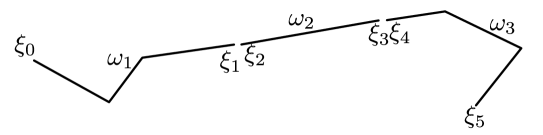
Figure 5. A depiction of an extended path $\Gamma$. The segment $\omega_{j}$ describes a piecewise linear path between the endpoints $\xi_{2j-2}$ and $\xi_{2j-1}$. The $\xi_{j}$ variables are phase space pairs $(x,p)$ describing the position and momentum of the particle at the boundary of the path segments.

Given an extended path we define an operator $O_{\Gamma}$ by

$$O_{\Gamma}=\mathinner{|{\xi_{0}}\rangle}\mathinner{\langle{\xi_{2N-1}}|}\prod_{\ell=1}^{N}\mathinner{\langle{\xi_{2\ell-2}|O_{\omega_{\ell}}|\xi_{2\ell-1}}\rangle},$$

so that including the sum over all possible collision numbers $0\leq k_{j}\leq k_{max}$ of each segment in the integral, we have

$$e^{iN\tau H}\approx\int O_{\Gamma}\mathop{}\!\mathrm{d}\Gamma,$$

where there is an error term in the approximation that is described in Section 3.

To write down the evolution channel ${\mathcal{E}}_{N\tau}$ we therefore arrive at an integral of the form

(1.15) $${\mathcal{E}}_{N\tau}[A]\approx\int{\mathbf{E}\,}O_{\Gamma^{+}}^{*}AO_{\Gamma^{-}}\mathop{}\!\mathrm{d}\Gamma^{+}\mathop{}\!\mathrm{d}\Gamma^{-}.$$

Before we take the expectation, we will split up the pairs of paths $(\Gamma^{+},\Gamma^{-})$ according to their geometric properties. The key result we will need is a description of the structure of the correlation partition of the paths in terms of the geometric features. This is done in Section 6, which characterizes the allowed partitions using ladders and anti-ladders. Here we simply provide a quick sketch. An example of a ladder partition on the disjoint union $[k]\sqcup[k]=[k]\times\{+,-\}$ is

$$P_{lad}=\{(j,+),(j,-)\}_{j\in[k]}.$$

An example of an anti-ladder partition on $[k]\sqcup[k]$ is the partition

$$P_{anti}=\{(j,+),(k+1-j,-)\}_{j\in[k]}.$$

The ladder and anti-ladder partitions are drawn in Figure 6

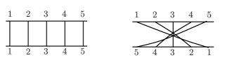
Figure 6. An example of a ladder and an anti-ladder partition with five rungs.

The main result of Section 6 is Lemma 6.16, which states that collisions that are not part of a geometric feature (so-called “typical collisions”) form part of either a ladder or an anti-ladder structure in the collision partition of $(\Gamma^{+},\Gamma^{-})$. Figure 7 illustrates the main result in a special case.

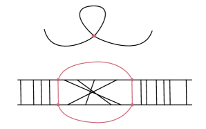
Figure 7. An example illustrating Lemma 6.16. On the top, a path that has a single recollision event. At the bottom, an example of a collision partition compatible with this single recollision event. Note that every collision that is not part of the recollision is either part of a ladder or an anti-ladder.

The next step is to partition the path integral according to the geometric information of the paths, which we encapsulate in a structure that we call a “skeleton” ${\mathcal{F}}(\Gamma^{+},\Gamma^{-})$. Given a skeleton ${\mathcal{F}}$, Lemma 6.16 allows us to construct a set of partitions ${\mathcal{Q}}_{\mathcal{F}}$ such that for any pair of paths $(\Gamma^{+},\Gamma^{-})$ with ${\mathcal{F}}(\Gamma^{+},\Gamma^{-})={\mathcal{F}}$, the collision partition $P(\Gamma^{+},\Gamma^{-})\in{\mathcal{Q}}_{\mathcal{F}}$. In fact, we have the stronger statement that for such pairs of paths,

(1.16) $${\mathbf{E}\,}O_{\Gamma^{+}}^{*}AO_{\Gamma^{-}}=\sum_{P\in{\mathcal{Q}}({\mathcal{F}})}{\mathbf{E}\,}_{P}O_{\Gamma^{+}}^{*}AO_{\Gamma^{-}},$$

where the sum is over partitions of the collision indices of $(\Gamma^{+},\Gamma^{-})$, and ${\mathbf{E}\,}_{P}$ is shorthand for a splitting of the expectation along the partition $P$.

Writing ${\mathbf{1}}_{{\mathcal{F}}}(\Gamma^{+},\Gamma^{-})$ for the indicator function that ${\mathcal{F}}(\Gamma^{+},\Gamma^{-})={\mathcal{F}}$, we then attain the following decomposition for the path integral:

$${\mathcal{E}}_{N\tau}[A] =\int{\mathbf{E}\,}O_{\Gamma^{+}}^{*}AO_{\Gamma^{-}}\mathop{}\!\mathrm{d}\Gamma^{+}\mathop{}\!\mathrm{d}\Gamma^{-}$$

$$=\sum_{{\mathcal{F}}}\int{\mathbf{1}}_{{\mathcal{F}}}(\Gamma^{+},\Gamma^{-}){\mathbf{E}\,}O_{\Gamma^{+}}^{*}AO_{\Gamma^{-}}\mathop{}\!\mathrm{d}\Gamma^{+}\mathop{}\!\mathrm{d}\Gamma^{-}$$

$$=\sum_{{\mathcal{F}}}\sum_{P\in{\mathcal{Q}}_{\mathcal{F}}}\int{\mathbf{1}}_{{\mathcal{F}}}(\Gamma^{+},\Gamma^{-}){\mathbf{E}\,}_{P}(O_{\Gamma^{+}})^{*}AO_{\Gamma^{-}}\mathop{}\!\mathrm{d}\Gamma^{+}\mathop{}\!\mathrm{d}\Gamma^{-}.$$

The benefit of decomposing the path integral in this way is that the expectation ${\mathbf{E}\,}_{P}$ splits in a known way. On the other hand there is now the challenge of dealing with the indicator function ${\mathbf{1}}_{\mathcal{F}}$. The reason this indicator functions causes a problem is not the discontinuity (this could be solved by using a smoother partition of unity) but rather the global nature of the constraints. In particular, ${\mathbf{1}}_{{\mathcal{F}}}(\Gamma^{+},\Gamma^{-})$ includes a product of indicator functions for each negative constraint, that is each pair of collisions that does not form a recollision or a tube event. The negative constraints are needed to be able to apply Lemma 6.16, but they make it difficult to exploit the cancellations needed. To get around this we use a special form of the inclusion-exclusion principle that is tailored to this purpose. In particular, in Section 7 we decompose the indicator function ${\mathbf{1}}_{\mathcal{F}}$ in the form

(1.17) $${\mathbf{1}}_{{\mathcal{F}}}=\sum_{{\mathcal{F}}^{\prime}\geq{\mathcal{F}}}G_{{\mathcal{F}},{\mathcal{F}}^{\prime}},$$

where we impose a partial ordering $\leq$ on skeletons, and where $G_{{\mathcal{F}},{\mathcal{F}}^{\prime}}$ is supported on the set of pairs $(\Gamma^{+},\Gamma^{-})$ such that ${\mathcal{F}}(\Gamma^{+},\Gamma^{-})\geq{\mathcal{F}}^{\prime}$. In the decomposition (1.17), the terms $G_{{\mathcal{F}},{\mathcal{F}}^{\prime}}$ depend only on the variables involving collisions that are in the support of the skeleton ${\mathcal{F}}^{\prime}$ (that is, collisions involved in a recollision, a cone event, or a tube event).

A challenge is to find a better way to handle the sum over partitions in ${\mathcal{Q}}_{\mathcal{F}}$. For this we introduce the concept of colored operators. Given a “coloring” function $\chi$ which assigns a unique color to each collision in $\Gamma$, we define the colored operator $O_{\Gamma}^{\chi}$ to be an analogue of $O_{\Gamma}$ which replaces each instance of the potential $V$ with an appropriately chosen independent copy of $V$. Then given a skeleton ${\mathcal{F}}$, we construct two sets of colors $\Psi^{+}({\mathcal{F}})$ and $\Psi^{-}({\mathcal{F}})$ so that

$$\sum_{P\in{\mathcal{Q}}({\mathcal{F}})}{\mathbf{E}\,}_{P}O_{\Gamma^{+}}^{*}AO_{\Gamma^{-}}=\sum_{\chi^{+}\in\Psi^{+}({\mathcal{F}})}\sum_{\chi^{-}\in\Psi^{-}({\mathcal{F}})}{\mathbf{E}\,}(O_{\Gamma^{+}}^{\chi^{+}})^{*}AO_{\Gamma^{-}}^{\chi^{-}}=:{\mathbf{E}\,}(O_{\Gamma^{+}}^{\Psi^{+}})^{*}AO_{\Gamma^{-}}^{\Psi^{-}}.$$

The precise definition of colored operators is given in Section 8, and the construction of colorings that reproduce the partition collection ${\mathcal{Q}}_{\mathcal{F}}$ is done in Section 9. The benefit of writing the expectation in this way is that we can use the “operator Cauchy-Schwartz” inequality

$$\|{\mathbf{E}\,}X^{*}AY\|_{op}\leq\|A\|_{op}\|{\mathbf{E}\,}X^{*}X\|_{op}^{1/2}\|{\mathbf{E}\,}Y^{*}Y\|_{op}^{1/2}$$

where $X$ and $Y$ are random operators, to simplify the estimation of the contribution from paths with skeleton ${\mathcal{F}}$. The result of this Cauchy-Schwartz procedure is depicted in Figure 8.

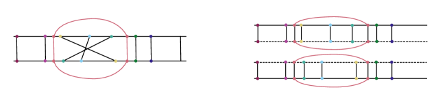
Figure 8. On the left, a partition with a collision coloring chosen so that matched collisions have the same color. When the operator Cauchy-Schwartz inequality is applied, a copy of the top and bottom rows are produced and matched to each other, converting the anti-ladder portion of the partition into a ladder (right).

More precisely, we will apply the operator Cauchy-Schwartz inequality to the operator

$${\mathcal{E}}_{{\mathcal{F}},{\mathcal{F}}^{\prime}}[A] :=\int G_{{\mathcal{F}},{\mathcal{F}}^{\prime}}(\Gamma^{+},\Gamma^{-})\sum_{P\in{\mathcal{Q}}_{\mathcal{F}}}{\mathbf{E}\,}_{P}(O_{\Gamma^{+}})^{*}AO_{\Gamma^{-}}\mathop{}\!\mathrm{d}\Gamma^{+}\mathop{}\!\mathrm{d}\Gamma^{-}$$

$$=\int G_{{\mathcal{F}},{\mathcal{F}}^{\prime}}(\Gamma^{+},\Gamma^{-}){\mathbf{E}\,}(O_{\Gamma^{+}}^{\Psi^{+}})^{*}AO_{\Gamma^{-}}^{\Psi^{-}}.\mathop{}\!\mathrm{d}\Gamma^{+}\mathop{}\!\mathrm{d}\Gamma^{-}.$$

To do this we first split $G_{{\mathcal{F}},{\mathcal{F}}^{\prime}}$ as a mixture of product functions of the form

(1.18) $$G_{{\mathcal{F}},{\mathcal{F}}^{\prime}}(\Gamma^{+},\Gamma^{-})=\int H(\theta)\chi_{{\mathcal{F}},{\mathcal{F}}^{\prime},\theta}^{+}(\omega)\chi_{{\mathcal{F}},{\mathcal{F}}^{\prime},\theta}^{-}(\omega^{\prime})\mathop{}\!\mathrm{d}\theta.$$

We also decompose the coloring sets $\Psi^{\pm}({\mathcal{F}},{\mathcal{F}}^{\prime})$ into carefully chosen components which are specified by a data structure called a scaffold, so we decompose

$$\Psi^{\pm}({\mathcal{F}},{\mathcal{F}}^{\prime})=\bigcup_{\operatorname{Scaff}\in{\mathcal{D}}^{\pm}({\mathcal{F}},{\mathcal{F}}^{\prime})}\Psi^{\pm}(\operatorname{Scaff}).$$

Then by applying the operator Cauchy-Schwartz inequality we arrive at the estimate

(1.19) $$\begin{split}\|{\mathcal{E}}_{{\mathcal{F}},{\mathcal{F}}^{\prime}}[A]\|_{op}&\leq\|A\|_{op}(\#{\mathcal{D}}^{+}({\mathcal{F}},{\mathcal{F}}^{\prime}))\sum_{\operatorname{Scaff}\in{\mathcal{D}}^{+}({\mathcal{F}},{\mathcal{F}}^{\prime})}\big{\|}\int|H(\theta)|{\mathbf{E}\,}(X^{+}_{\operatorname{Scaff},\theta})^{*}(X^{+}_{\operatorname{Scaff},\theta})\mathop{}\!\mathrm{d}\theta\big{\|}_{op}^{1/2}\\ &\qquad(\#{\mathcal{D}}^{-}({\mathcal{F}},{\mathcal{F}}^{\prime}))\sum_{\operatorname{Scaff}\in{\mathcal{D}}^{-}({\mathcal{F}},{\mathcal{F}}^{\prime})}\big{\|}\int|H(\theta)|{\mathbf{E}\,}(X^{-}_{\operatorname{Scaff},\theta})^{*}(X^{-}_{\operatorname{Scaff},\theta})\mathop{}\!\mathrm{d}\theta\big{\|}_{op}^{1/2},\end{split}$$

where

$$X^{\pm}_{\operatorname{Scaff},\theta}:=\int\chi_{{\mathcal{F}},{\mathcal{F}}^{\prime},\theta}^{\pm}(\omega)\sum_{\psi\in\Psi^{\pm}(\operatorname{Scaff})}O_{\Gamma}^{\psi}\mathop{}\!\mathrm{d}\Gamma.$$

This calculation involving the Cauchy-Schwartz inequality is done more carefully in Section 10.

The point of defining the scaffolds is that we can arrange that the operators ${\mathbf{E}\,}(X^{\pm}_{\operatorname{Scaff},\theta})^{*}(X^{\pm}_{\operatorname{Scaff},\theta})$ involve sums over partitions that are formed only from ladders, not anti-ladders. The point is that ladder partitions have a semigroup structure in the sense that the concatenation of two ladders is a ladder. We use this structure to more easily use exact cancellations. More precisely, we use the fact that the ladder partitions form a good approximation to the evolution ${\mathcal{E}}_{\tau}$ at subkinetic times and the fact that ${\mathcal{E}}_{\tau}$ is a contraction in operator norm in order to obtain the bounds we need. These bounds are proven in Section 12.

We also point out that the use of Cauchy-Schwartz in this way is lossy, but it only loses a factor of $N^{C\|{\mathcal{F}}\|}$. We can afford to lose this factor because the operator norm appearing in the right hand side (1.19) will have order ${\varepsilon}^{c\|{\mathcal{F}}\|}$. Roughly this is because we obtain a factor of ${\varepsilon}$ for each special geometric event described in ${\mathcal{F}}$. A careful argument is needed to ensure that one can obtain additional factors of ${\varepsilon}$ for each recollision (say) in an integral over paths containing multiple recollisions, and this is done in Section 11.

1.4. An abbreviated review of related works

Here we point out some related works, making no attempt at providing a complete review of the rich field of dynamics in random fields.

The rigorous study of the random Schrodinger equation began with the previously mentioned work of H. Spohn [29]. As mentioned previously, Spohn’s analysis was extended to the kinetic time in [18] and then to diffusive times in [15, 16]. Each of these papers considers the convergence in mean of the Wigner function to the solution of a kinetic equation. A natural question is to understand the size of the fluctuations of the Wigner function. An analysis was carried out by T. Chen in [8] which showed that in fact that the $r$-th moments of the Wigner function are bounded for any $r<\infty$. Chen’s analysis was later improved by M. Butz in [7]. We also point out the work of J. Lukkarinen and H. Spohn in [24], which shows that the diagrammatic methods applied to the Schrödinger equation can also be used to derive kinetic equations for a random wave equation. See the review [3] for a more complete discussion of the kinetic regime for waves in a random medium.

Other regimes of interest are the homogenization regime in which the wavelength of the initial condition is substantially longer than the decorrelation length scale of the potential. This was studied by G. Bal and N. Zhang in [31], where a homogenized equation with a constant effective potential is shown to describe the evolution of the average wave function. This limit was further studied by T. Chen, T. Komorowski, and L. Ryzhik in [9]. An entirely different approach to the study of the average wave function in the kinetic regime was introduced by M. Duerinckx and C. Shirley in [12]. There the authors use ideas from spectral theory to understand the evolution operator, and are able to show with this method that the average wave function decays exponentially on the kinetic time scale.

The high frequency regime, in which the wavelength of the initial condition is much shorter than the decorrelation length of the potential, was considered by G. Bal, T. Komorowski, and L. Ryzhik in [2]. There the authors derive a Fokker-Planck equation for the evolution of the Wigner function.

The study of the random Schrodinger equation falls into a larger body of work of understanding the emergence of apparently irreversible phenomena from reversible dynamics [28]. From this point of view, the random Schrodinger equation is simply the one-particle quantum mechanical manifestation of a larger phenomenon.

The classical version is the stochastic acceleration problem given by the ordinary differential equation

$$\ddot{x}=-{\varepsilon}\nabla V(x)$$

where again $V$ is a stationary random potential. Diffusive behavior for the stochastic acceleration problem was first demonstrated by H. Kesten and G. Papanicolau in [20] for dimensions $d\geq 3$. For a special class of potentials their argument was then applied to the two dimensional case by D. Dürr, S. Goldstein, and J. Lebowitz in [13], and then T. Komorowski and L. Ryzhik lifted the restriction on the potentials in [21]. The argument used by Kesten and Papanicolau inspired the semigroup approach taken in this paper. The connection is that Kesten and Papanicolau define a modified version of the stochastic acceleration problem in which unwanted correlations are ruled out by fiat. They then show that this modified evolution is unlikely to have recollisions after all, and therefore is close to the original evolution. In a similar way we define an evolution (the refreshed evolution ${\mathcal{E}}_{s}^{m}$) which removes unwanted correlations and use properties of this evolution to study the true evolution ${\mathcal{E}}_{ms}$. Although this is where the similarities end, it does seem that a further unification of the proof techniques may be possible one day.

There are a number of other classical models of particles moving in a random environment. A popular model is the Lorentz gas, in which a billiard travels through ${\mathbf{R}}^{d}$ with some obstacles placed according to a Poisson process. A pioneering paper in the study of the Lorentz gas is [4] where a linear Boltzmann equation is derived at the Boltzmann-Grad limit of the model. A review of this model is provided in [11]. We refer the reader also to some exciting recent developments in this field [1, 22, 26]. It seems that the classical models of particles moving in random environment contain many of the same difficulties of understanding the quantum evolution. A deeper understanding of the phase-space path integral may lead us to a better understanding of the relationship between the classical and quantum problems.

The random Schrodinger equation is also closely related to wave-kinetic theory in which one studies the evolution of random waves with a nonlinear interaction (see [27] for a physically-motivated introduction to this theory). A pioneering work in this field is the paper of Lukkarinen and Spohn [25], in which a wave kinetic equation is derived for the nonlinear Schrodinger equation for initial conditions that are perturbations of an equilibrium state. In a series of works [19, 5, 10, 6] a wave kinetic equation was derived for the nonlinear Schrodinger equation on a torus with more general initial conditions. Independently, in [30] a wave kinetic equation was derived for the Zakharov-Kuznetsov equation on ${\mathbf{R}}^{d}$ for $d\geq 2$. Each of these works follows the traditional strategy of writing out a diagrammatic expansion for the solution and finding sources of cancellation in the error terms and comparing the main terms to a perturbative expansion of the kinetic equation. It seems possible that the wavepacket decomposition used in this paper and the approximate-semigroup argument could be used to make further progress in wave-kinetic theory.

1.5. Acknowledgements

The author is very grateful to Lenya Ryzhik for years of support, advice, and many clarifying discussions. The author also warmly thanks Minh-Binh Tran for many helpful conversations about the paper. The author is supported by the Fannie and John Hertz Foundation.

2. More detailed outline of the proof

In this section we lay out the main lemmas used to prove Theorem 1.1.

The proof involves analysis of three time scales. The first time scale is the time ${\varepsilon}^{-1.5}$ during which the particle is unlikely to scatter at all and in particular is unlikely to experience more than one scattering event. The main result we need from this time scale shows that the linear Boltzmann equation agrees with the evolution ${\mathcal{E}}_{s}$ with an error that is very small in operator norm. This calculation is standard and is reproduced in Appendix A for the sake of completeness. The calculation only involves two terms from the Duhamel expansion of $e^{-itH}$ so there are no combinatorial difficulties. propositionshorttime There exists $\theta(d)>0$ such that the following holds: Let $a_{0}\in C^{2d+1}$ be an observable supported on the set $\{(x,p)||p|>{\varepsilon}^{\theta}\}$, and suppose that $a_{s}$ solves the linear Boltzmann equation (1.8). Then for $\sigma\leq{\varepsilon}^{-1.5}$,

(2.1) $$\|\operatorname{Op}(a_{\sigma})-{\mathcal{E}}_{\sigma}[\operatorname{Op}(a_{0})]\|_{op}{\,\lesssim\,}{\varepsilon}^{2.1}\sigma\|a_{0}\|_{C^{2d+1}_{{\varepsilon}^{-1},{\varepsilon}^{-0.25}}}.$$

To use Proposition 2 along with the semigroup approximation strategy, we need the following regularity result for the short time evolution of the linear Boltzmann equation.

Lemma 2.1.

There exists $\theta=\theta(d)>0$ such that the following holds: Let $a_{s}$ solve the linear Boltzmann equation (1.8) and $\operatorname{supp}a_{0}\subset\{(x,p)\mid|p|\geq{\varepsilon}^{\theta}\}$. Then for $s\leq{\varepsilon}^{-2.05}$,

$$\|a_{s}\|_{C^{2d+1}_{{\varepsilon}^{-1},{\varepsilon}^{-0.25}}}\leq C\|a_{0}\|_{C^{2d+1}_{{\varepsilon}^{-1},{\varepsilon}^{-0.5}}}.$$

Lemma 2.1 is proven with a simple and suboptimal argument in Appendix D, where we prove a slightly stronger version in Lemma D.1.

Using Proposition 2 and Lemma 2.1 we can prove that the “$\sigma$-refreshed” evolution ${\mathcal{E}}_{\sigma}^{n}$ approximates the linear Boltzmann equation up to a diffusive timescale.

Corollary 2.2.

For $\sigma={\varepsilon}^{-1.5}$ and $m\in{\mathbb{N}}$ such that $m\sigma\leq{\varepsilon}^{-2.05}$, and $a_{s}$ solving (1.8),

(2.2) $$\|{\mathcal{E}}_{\sigma}^{m}[\operatorname{Op}(a_{0})]-\operatorname{Op}(a_{m\sigma})\|_{op}\leq C{\varepsilon}^{2.1}m\sigma\|a_{0}\|_{C^{2d+1}_{{\varepsilon}^{-1},{\varepsilon}^{-0.5}}}.$$

Proof.

We define the quantity

$$F_{j}:=\sup_{\|a_{0}\|_{C^{2d+1}_{{\varepsilon}^{-1},{\varepsilon}^{-0.5}}}=1}\|{\mathcal{E}}_{\sigma}^{j}[\operatorname{Op}(a_{0})]-\operatorname{Op}(a_{j\sigma})\|_{op}.$$

By Proposition 2, $F_{1}\leq C{\varepsilon}^{2.1}\sigma$. To obtain a bound for $F_{j+1}$ from $F_{j}$ we write

$$\|{\mathcal{E}}_{\sigma}^{m}[\operatorname{Op}(a)]-\operatorname{Op}(a_{m\sigma})\|_{op}\leq\|{\mathcal{E}}_{\sigma}[\operatorname{Op}(a_{(m-1)\sigma})]-\operatorname{Op}(a_{m\sigma})\|_{op}+\|{\mathcal{E}}_{\sigma}^{m}[\operatorname{Op}(a)]-{\mathcal{E}}_{\sigma}[\operatorname{Op}(a_{(m-1)\sigma})]\|_{op}.$$

The first quantity is bounded using Proposition 2 and Lemma 2.1. The second term is bounded by $F_{j}$ using the fact that ${\mathcal{E}}_{\sigma}$ is linear and is a contraction in the operator norm:

$$\|{\mathcal{E}}_{\sigma}[A]\|_{op}=\|{\mathbf{E}\,}e^{i\sigma H}Ae^{-i\sigma H}\|_{op}\leq{\mathbf{E}\,}\|e^{i\sigma H}Ae^{-i\sigma H}\|_{op}=\|A\|_{op}.$$

Therefore we obtain the bound

$$F_{j+1}\leq F_{j}+C{\varepsilon}^{2.1}\sigma.$$

In particular,

$$F_{m}\leq C{\varepsilon}^{2.1}m\sigma,$$

so (2.2) follows. ∎

The more substantial component of the proof of Theorem 1.1 is the approximate semigroup property relating the “refreshed” evolution ${\mathcal{E}}_{\sigma}^{M}$ to the correct evolution channel ${\mathcal{E}}_{M\sigma}$. For the purposes of proving an approximate semigroup property it is more convenient to work with the “wavepacket quantization” defined by.

$$\operatorname{Op}(a):=\int_{{\mathbf{R}}^{d}}\mathinner{|{\xi}\rangle}\mathinner{\langle{\xi}|}a(\xi)\mathop{}\!\mathrm{d}\xi.$$

In Appendix C we will show that the wavepacket quantization is close to the Weyl quantization, in the sense that

$$\|\operatorname{Op}(a)-\operatorname{Op}^{w}(a)\|_{op}\leq{\varepsilon}^{0.05}\|a\|_{C^{2d+1}_{{\varepsilon}^{-1},{\varepsilon}^{-0.1}}}.$$

In general, we will be interested in operators of the form

$$A=\int\mathinner{|{\xi}\rangle}\mathinner{\langle{\eta}|}a(\xi,\eta)\mathop{}\!\mathrm{d}\xi$$

with kernel $a(\xi,\eta)$ satisfying $|a(\xi,\eta)|\leq C\|A\|_{op}$ and supported on near the diagonal. To quantify this we introduce the distance $d_{r}$ on ${{\mathbf{R}}^{2d}}$ so that, writing $\xi=(\xi_{x},\xi_{p})$ and $\eta=(\eta_{x},\eta_{p})$,

$$d_{r}(\xi,\eta):=r^{-1}|\xi_{x}-\eta_{x}|+r|\xi_{p}-\eta_{p}|.$$

More precisely, we are interested in families of good operators, defined below.

Definition 2.3 (Good operators).

An operator $A\in\mathcal{B}(L^{2}({\mathbf{R}}^{d}))$ is said to be $(C_{1},C_{2},\delta)$-good if there exists a function $a:{{\mathbf{R}}^{2d}}\times{{\mathbf{R}}^{2d}}\to{\mathbf{C}}$ supported in the set

$$\operatorname{supp}a\subset\{(\xi,\eta)\in{{\mathbf{R}}^{2d}}\times{{\mathbf{R}}^{2d}}\mid d_{r}(\xi,\eta)<C_{1},|\xi_{p}|\geq{\varepsilon}^{\theta}-C_{2}{\varepsilon}\}$$

such that

$$\|A-\int a(\xi,\eta)\mathinner{|{\xi}\rangle}\mathinner{\langle{\eta}|}\mathop{}\!\mathrm{d}\xi\mathop{}\!\mathrm{d}\eta\|_{op}\leq\delta.$$

Note that the rank one projection onto a wavepacket $\mathinner{|{\xi}\rangle}\mathinner{\langle{\xi}|}$ is (formally) a $(0,0,0)$-good operator if $|\xi_{p}|\geq{\varepsilon}^{\theta}$, but its Wigner transform has smoothness only at the microscopic scale $(r,r^{-1})$. Similarly if $a\in C^{2d+1}$ is an observable supported on $\{(x,p)||p|\geq{\varepsilon}^{\theta}\}$, then the wavepacket quantization $\operatorname{Op}(a)$ is a $(0,0,0)$-good operator. Moreover, by (C.6) we have that $\operatorname{Op}^{w}(a)$ is a $(0,0,{\varepsilon}^{1/2})$-good operator if $a\in C^{2d+1}_{{\varepsilon}^{-1},{\varepsilon}^{-1/2}}$.

The first step in the proof of the approximate semigroup property is to verify a semigroup property up to times ${\varepsilon}^{-2+\kappa/2}$.

Proposition 2.4.

If $A$ is a $(C_{1},C_{2},\delta)$-good operator with $C_{1}\leq{\varepsilon}^{-0.1}$ and $C_{2}\leq\frac{1}{2}{\varepsilon}^{\theta}$ and ${\varepsilon}^{-1.5}<s<{\varepsilon}^{-2+\kappa/2}$ then

$$\|{\mathcal{E}}_{2s}[A]-{\mathcal{E}}_{s}^{2}[A]\|_{op}\leq{\varepsilon}^{2.1}s\|A\|_{op}+2\delta.$$

and moreover ${\mathcal{E}}_{s}[A]$ is a $(C_{1}+|\log{\varepsilon}|^{10},C_{2}-10^{3}{\varepsilon},\delta+{\varepsilon}^{100})$-good operator.

Proposition 2.4 is proved by first comparing ${\mathcal{E}}_{s}$ to the expectation over ladders, and then observing that the semigroup property holds for ladders. The first step is done in Section 4 where we prove Proposition 4.10. The derivation of Proposition 2.4 from Proposition 4.10 is explained by Lemma 12.2.

Using Proposition 2.4 we can prove a comparison result between the linear Boltzmann equation and the quantum evolution for times up to ${\varepsilon}^{-2+\kappa/10}$.

Corollary 2.5.

If $A$ is a $(C_{1},C_{2},\delta)$-good operator with $C_{1}\leq\frac{1}{2}{\varepsilon}^{-0.1}$ and $C_{2}\leq{\varepsilon}^{\theta}$ then with $\sigma={\varepsilon}^{-1.5}$,

$$\|{\mathcal{E}}_{\sigma}^{m}[A]-{\mathcal{E}}_{m\sigma}[A]\|_{op}\leq C_{\kappa}{\varepsilon}^{2.1}\sigma\|A\|_{op}+2\delta+{\varepsilon}^{20}$$

for $m$ such that $m\sigma\leq{\varepsilon}^{-2+\kappa/2}$.

Proof.

We perform an iteration, defining the error

$$E_{m}:=\sup_{\begin{subarray}{c}\|A\|_{op}=1\\ A\text{ is }(C_{1}-K_{1}m,C_{2}+K_{2}m,\beta-\delta m){-good}\end{subarray}}\|{\mathcal{E}}_{2^{m}\sigma}[A]-{\mathcal{E}}_{\sigma}^{2^{m}}[A]\|_{op},$$

where we choose $C_{1}=\frac{1}{2}{\varepsilon}^{-0.1}$, $K_{1}=|\log{\varepsilon}|^{10}$, $C_{2}=\frac{1}{4}{\varepsilon}^{0.1}$, $K_{2}=10^{3}{\varepsilon}$, $\beta={\varepsilon}^{100}$, and $\delta={\varepsilon}^{100}$. Let ${\mathcal{A}}_{m}$ be the class of admissible operators in the supremum defining $E_{m}$. The significant point about ${\mathcal{A}}_{m}$ is that ${\mathcal{E}}_{s}[A]\in{\mathcal{A}}_{m}$ when $A\in{\mathcal{A}}_{m+1}$. To find a recursion for $E_{m}$, we write

(2.3) $$\begin{split}\|{\mathcal{E}}_{2^{m+1}s}[A]-{\mathcal{E}}_{s}^{2^{m+1}}[A]\|_{op}&\leq\|{\mathcal{E}}_{2^{m+1}s}[A]-{\mathcal{E}}_{2^{m}s}^{2}[A]\|_{op}+\|{\mathcal{E}}_{2^{m}s}^{2}[A]-{\mathcal{E}}_{s}^{2^{m+1}}[A]\|_{op}\\ &\leq\|{\mathcal{E}}_{2^{m+1}s}[A]-{\mathcal{E}}_{2^{m}s}^{2}[A]\|_{op}+\|{\mathcal{E}}_{2^{m}s}[{\mathcal{E}}_{2^{m}s}[A]-{\mathcal{E}}_{s}^{2^{m}}[A]]\|_{op}\\ &\qquad\qquad+\|({\mathcal{E}}_{2^{m}s}-{\mathcal{E}}_{s}^{2^{m}}){\mathcal{E}}_{s}^{2^{m}}[A]\|_{op}.\end{split}$$

Since ${\mathcal{E}}_{s}$ is a contraction in the operator norm, and since ${\mathcal{E}}_{s}$ maps ${\mathcal{A}}_{m+1}$ into ${\mathcal{A}}_{m}$ we have by Proposition 2.4 that

$$\|{\mathcal{E}}_{2^{m+1}s}[A]-{\mathcal{E}}_{s}^{2^{m+1}}[A]\|_{op}\leq(({\varepsilon}^{2.1}2^{m}s)\|A\|_{op}+2\delta)+E_{m}.$$

Taking a supremum over $A$ we obtain the relation

$$E_{m+1}\leq{\varepsilon}^{2.1}2^{m}\sigma+2E_{m}.$$

Since $E_{0}=0$, we obtain

$$E_{m}\leq m{\varepsilon}^{2.1}2^{m}\sigma.$$

∎

The remaining ingredient needed to prove Theorem 1.1 is a semigroup property that holds up to diffusive times. This is substantially more difficult than establishing the semigroup property for subkinetic times because of the need for resummation in the Duhamel series. The main result is the following.

Proposition 2.6.

There exists $\kappa=\kappa(d)$ such that the following holds: If $A$ is a $({\varepsilon}^{-0.1},\frac{1}{2}{\varepsilon}^{0.1},\delta)$-good operator, then with $\tau={\varepsilon}^{-2+\kappa/2}$ and $N=\lfloor{\varepsilon}^{-\kappa}\rfloor$,

$$\|{\mathcal{E}}_{N\tau}[A]-{\mathcal{E}}_{\tau}^{N}[A]\|_{op}\leq{\varepsilon}^{c\kappa}\|A\|_{op}+2\delta.$$

Having sketched the argument proving the main result, we now outline the remaining sections in the paper. In Section 3 we explain the phase space path integral approximation we use throughout the paper. Then in Section 4 we introduce the ladder superoperator ${\mathcal{L}}_{s}$ which is a main character in the derivation of the approximate semigroup property. Section 4 contains the bulk of the proof of Proposition 2.4 and contains most of the main ideas of the paper.

The remaining sections in the paper are dedicated to the proof of Proposition 2.6. In Section 5 we write down the path integral used to represent the solution operator up to this time. Then in Section 6 we clarify the relationship between the geometry of paths and the combinatorial features of their collision partitions. Then in Section 7 we split up the path integral according to the geometry of the paths. To exploit the combinatorial structure of the correlation partition, we introduce the formalism of colored operators in Section 8 and Section 9. Then in Section 10 we finally write out our version of a “diagrammatic expansion” (which is different than previous expansions in that the first term of the expansion for ${\mathcal{E}}_{N\tau}[A]$ is the refreshed evolution ${\mathcal{E}}_{\tau}^{N}[A]$). The diagrams are bounded in Section 11.

The remaining sections contain proofs of more technical results needed throughout the argument, and are referenced as needed.

3. A sketch of the derivation of the path integral

In this section we state the precise version of the phase-space path integral alluded to in Section 1.3. The proofs of the assertions made in this section are given in Sections 13, 14, and 15.

The first step is to write out an expansion for $e^{-isH}$ that is valid for times $s\leq\tau:={\varepsilon}^{-2+\kappa/2}$ in terms of paths. More precisely, a path $\omega=({\mathbf{s}},{\mathbf{p}},{\mathbf{y}})$ having $k$ collisions is a tuple containing a list of collision invervals ${\mathbf{s}}\in{\mathbf{R}}_{+}^{k+1}$ satisfying $\sum_{j=0}^{k}s_{j}=s$, momenta ${\mathbf{p}}\in({\mathbf{R}}^{d})^{k+1}$, and collision locations ${\mathbf{y}}\in({\mathbf{R}}^{d})^{k}$. Each path $\omega$ is associated to the operator $O_{\omega}$ defined by

$${\widehat{O_{\omega}\psi}}=\delta_{p_{k}}{\widehat{\psi}}(p_{0})e^{i\varphi(\omega)}\prod_{j=1}^{k}{\widehat{V_{y_{j}}}}(p_{j}-p_{j-1}),$$

where $\varphi(\omega)$ is the phase function

$$\varphi(\omega)=\sum_{j=0}^{k}s_{j}|p_{j}|^{2}/2+\sum_{j=1}^{k}y_{j}\cdot(p_{j}-p_{j-1}).$$

In Dirac notation, we express $O_{\omega}$ as

(3.1) $$O_{\omega}=\mathinner{|{p_{k}}\rangle}\mathinner{\langle{p_{0}}|}e^{i\varphi(\omega)}\prod_{j=1}^{k}{\widehat{V_{y_{j}}}}(p_{j}-p_{j-1}).$$

Here $V_{y}(x)=V(x-y)\chi^{V}(x)$ is a localized and shifted version of the potential, with localization $\chi^{V}$ having width $r$ and satisfying $\int\chi^{V}=1$.

Let $\Omega_{k}(s)$ denote the space of paths with $k$ collisions and duration $s$,

$$\Omega_{k}(s)=\triangle_{k}(s)\times({\mathbf{R}}^{d})^{k+1}\times({\mathbf{R}}^{d})^{k},$$

where $\triangle_{k}(s)\subset{\mathbf{R}}_{+}^{k+1}$ is the set of tuples of time intervals summing to $s$,

$$\triangle_{k}(s)=\{{\mathbf{s}}=(s_{0},\cdots,s_{k})\in{\mathbf{R}}_{+}^{k+1}\mid\sum_{j=0}^{k}s_{j}=s\}.$$

We will see in Section 13 that the Duhamel expansion can be formally written

$$e^{isH}=\sum_{k=0}^{\infty}T_{k}:=\sum_{k=0}^{\infty}\int_{\Omega_{k}(s)}O_{\omega}\mathop{}\!\mathrm{d}\omega.$$

In this integral there is no need for the collision locations ${\mathbf{y}}$ to have any relationship with the variables ${\mathbf{s}}$ and ${\mathbf{p}}$. There is however significant cancellation due to the presence of the phase $e^{i\varphi(\omega)}$. For example, by integrating by parts in the $p_{j}$ variables and using the identity,

$$\partial_{p_{j}}\varphi(\omega)=y_{j}+s_{j}p_{j}-y_{j+1},$$

we can reduce the path integral to paths which satisfy

$$|y_{j+1}-(y_{j}+s_{j}p_{j})|\lessapprox r.$$

Integration by parts in the $s_{j}$ is somewhat more delicate because of the hard constraint $\sum s_{j}=\tau$. By decomposing this hard constraint as a sum of softer constraints, we can impose a cutoff on the weaker conservation of kinetic energy condition

$$||p_{j}|^{2}/2-|p_{j^{\prime}}|^{2}/2|\lessapprox\max\{|p_{j}|r^{-1},s_{j}^{-1},s_{j^{\prime}}^{-1}\}.$$

The integration by parts argument will allow us to construct a function $\chi^{path}$ supported on the set of such “good” paths and for which

$$T_{k}\approx\int_{\Omega_{k}(s)}\chi^{path}(\omega)O_{\omega}\mathop{}\!\mathrm{d}\omega,$$

with an error that is negligible in operator norm. To be more precise, given a tolerance $\alpha$ (which we set to be $|\log{\varepsilon}|^{10}$), we define

(3.2) $$\begin{split}\Omega_{\alpha,k}(s)=\{({\mathbf{s}},{\mathbf{p}},{\mathbf{y}})\in\Omega_{k}(s)\mid&|y_{j+1}-(y_{j}+s_{j}p_{j})|\leq\alpha r\text{ for all }j\in[1,k-1]\text{ and }\\ &||p_{j}|^{2}/2-|p_{j^{\prime}}|^{2}/2|\leq\alpha\max\{s_{j^{\prime}}^{-1},s_{j}^{-1},|p_{j}|r^{-1},\alpha r^{-2}\}\text{ for all }j,j^{\prime}\in[0,k]\}.\end{split}$$

Within $\Omega_{\alpha,k}(s)$ we also define the subset

(3.3) $$\begin{split}\Omega_{\alpha,k}(t;\xi,\eta):=\{({\mathbf{s}},{\mathbf{p}},{\mathbf{y}})\in\Omega_{\alpha,k}(t)\mid&|y_{1}-(\xi_{x}+s_{0}p_{0})|\leq\alpha r,|\eta_{x}-(y_{k}+s_{k}p_{k})|\leq\alpha r,\\ &|p_{0}-\xi_{p}|\leq\alpha r^{-1},\text{ and }|p_{k}-\eta_{p}|\leq\alpha r^{-1}\},\end{split}$$

where $\xi,\eta\in{{\mathbf{R}}^{2d}}$ with $\xi=(\xi_{x},\xi_{p})$ and $\eta=(\eta_{x},\eta_{p})$.

The following lemma is simply a careful application of integration by parts, and is done in Section 13.

Lemma 3.1.

There exists a cutoff function $\chi\in C^{\infty}(\Omega_{k}(\tau)\times{{\mathbf{R}}^{2d}}\times{{\mathbf{R}}^{2d}})$ supported in the set

$$\operatorname{supp}\chi\subset\{(\omega,\xi,\eta)\mid\omega\in\Omega_{\alpha,k}(\tau;\xi,\eta)\}$$

such that, with

(3.4) $$T_{k}^{\chi}(\tau):=(i{\varepsilon})^{k}\int_{\Omega_{k}(\tau)\times{{\mathbf{R}}^{2d}}\times{{\mathbf{R}}^{2d}}}\mathinner{|{\eta}\rangle}\mathinner{\langle{\xi}|}\chi(\omega,\xi,\eta)\mathinner{\langle{\eta|O_{\omega}|\xi}\rangle}\mathop{}\!\mathrm{d}\omega\mathop{}\!\mathrm{d}\xi\mathop{}\!\mathrm{d}\eta,$$

we have the approximation

(3.5) $$\|T_{k}^{\chi}-T_{k}\|_{op}\leq{\varepsilon}^{-C_{d}k}\|V\|_{C^{10d}}^{Ck}\exp(-c\alpha^{0.99}).$$

The point of Lemma 3.1 is that it allows us to neglect the contribution of “physically unreasonable paths” – those that either badly violate conservation of kinetic energy or the transport constraints $y_{k+1}\approx y_{k}+s_{k}p_{k}$.

We remark that Lemma 3.1 is deterministic in the sense that that the conclusion holds for all potentials, and when we apply it we will simply need moment bounds for the $C^{10d}$ norm of the potential (after being cutoff to a ball of large radius). With the choice $\alpha=|\log{\varepsilon}|^{10}$, and assuming that $\|V\|_{C^{10d}}\leq{\varepsilon}^{-100}$ (say), the right hand side is still $O({\varepsilon}^{K})$ for any $K>0$.

Having given a description to the collision operators $T_{k}$, it remains to estimate moments of the form ${\mathbf{E}\,}\|T_{k}^{\chi}\|_{op}^{M}$, for which we use the moment method:

$${\mathbf{E}\,}\|T_{k}^{\chi}\|_{op}^{2M}\leq{\mathbf{E}\,}\operatorname{tr}((T_{k}^{\chi})^{*}T_{k}^{\chi})^{M}.$$

Note that this step is where the cutoff on the potential is crucial – without the cutoff $\chi_{R}$ the trace above would be infinite. In Section 14 we prove Lemma 14.1, which states that

$$\Big{(}{\mathbf{E}\,}\|T_{k}^{\chi}(s)\|_{op}^{2M}\Big{)}^{1/M}\leq R^{C/m}{\varepsilon}^{2}s\,\,(C(kM)^{C}|\log{\varepsilon}|^{10}).$$

The presence of the factor $(km)^{C}$ makes this bound unsuitable for reaching diffusive time scales. However this bound is good enough to approximate $e^{isH}$ by $e^{-is\Delta/2}$ for times $s\leq{\varepsilon}^{-1.1}$ (say). We use this result in Section 15 to define a modified operator $T_{k,\rho}^{\chi}$ which involves a first short period of free evolution. More precisely, given a time $\sigma>0$ we construct a function $\rho_{\sigma}\geq 0$ that is supported on the interval $[\sigma 2\sigma]$, is Gevrey regular, and satisfies $\int\rho_{\sigma}=1$. Then we define

$${\widetilde{U}}_{\tau,\sigma}:=\int_{\sigma}^{2\sigma}\int_{\sigma}^{2\sigma}e^{is\Delta/2}e^{-i(\tau-s-s^{\prime})H}e^{is^{\prime}\Delta/2}\rho_{\sigma}(s)\rho_{\sigma}(s^{\prime})\mathop{}\!\mathrm{d}s\mathop{}\!\mathrm{d}s^{\prime}.$$

We will fix for the remainder of the paper $\sigma={\varepsilon}^{-1.5}$. In Section 15 we use Lemma 3.1 to prove Lemma 15.1, which justifies the approximation

$$\|{\mathcal{E}}_{N\tau}[A]-{\mathbf{E}\,}({\widetilde{U}}_{\tau,\sigma}^{*})^{N}A{\widetilde{U}}_{\tau,\sigma}^{N}\|_{op}\leq{\varepsilon}^{0.2}.$$

This will allow us to restrict the path integral to a space of paths which do not have a collision too close to either endpoint,

$$\Omega_{k,\alpha}(\tau,\sigma;\xi,\eta):=\{(\omega,\xi,\eta)\in\Omega_{k,\alpha}(\tau;\xi,\eta)\mid s_{0}\geq\sigma\text{ and }s_{k}\geq\sigma\}.$$

The operator ${\widetilde{U}}_{\tau,\sigma}$ also has a path integral expansion in terms of collision operators $T_{k}^{\chi,\sigma}$, which in addition to having the smooth cutoff $\chi$ have a cutoff enforcing that $\omega\in\Omega_{k,\alpha}(\tau,\sigma;\xi,\eta)$.

Combining the above arguments we obtain the following approximation result for the evolution operator ${\widetilde{U}}_{\tau,\sigma}$.

Proposition 3.2.

There exists a bounded smooth function $\chi_{\sigma}\in C^{\infty}(\Omega_{k}(\tau)\times{\mathbf{R}}^{2d}\times{\mathbf{R}}^{2d})$ supported in the set

$$\operatorname{supp}(\chi_{\sigma})\subset\Omega_{\alpha,k}(\tau,S;\xi,\eta):=\{(\omega,\xi,\eta)\mid\omega\in\Omega_{k,\alpha}(\tau;\xi,\eta)\text{ and }s_{0}\geq{\varepsilon}^{-1.6},\text{ and }s_{k}\geq{\varepsilon}^{-1.6}\},$$

and such that, with

(3.6) $$T_{k}^{\chi,\sigma}:=(i{\varepsilon})^{k}\int_{\Omega_{k}(\tau)\times{\mathbf{R}}^{2d}\times{\mathbf{R}}^{2d}}\mathinner{|{\eta}\rangle}\mathinner{\langle{\xi}|}\chi_{\sigma}(\omega,\xi,\eta)\mathinner{\langle{\eta|O_{\omega}|\xi}\rangle}\mathop{}\!\mathrm{d}\omega\mathop{}\!\mathrm{d}\xi\mathop{}\!\mathrm{d}\eta,$$

we have the Duhamel expansion

$${\widetilde{U}}_{\tau,\sigma}:=\sum_{k=0}^{k_{max}}T_{k}^{\chi,\sigma}+R_{k_{max}}^{\chi,\sigma},$$

where the remainder $R_{k_{max}}^{\chi,\rho}$ has the expression

(3.7) $$R_{k_{max}}^{\chi,\sigma}:=(i{\varepsilon})^{k}\int_{0}^{\tau}\mathop{}\!\mathrm{d}s\int_{\Omega_{k_{max}}(s)\times{\mathbf{R}}^{2d}\times{\mathbf{R}}^{2d}}e^{i(\tau-s)H}\mathinner{|{\eta}\rangle}\mathinner{\langle{\xi}|}\chi_{\sigma}(\omega,\xi,\eta)\mathinner{\langle{\eta|O_{\omega}|\xi}\rangle}\mathop{}\!\mathrm{d}\omega\mathop{}\!\mathrm{d}\xi\mathop{}\!\mathrm{d}\eta,$$

and

(3.8) $$\left({\mathbf{E}\,}\|e^{i\tau H}-{\widetilde{U}}_{\tau,\sigma}\|_{op}^{{\varepsilon}^{-0.1}}\right)^{{\varepsilon}^{0.1}}\leq{\varepsilon}^{0.3}$$

We use the operator ${\widetilde{U}}_{\tau,\sigma}=:U_{\tau,\sigma}+R_{k_{max}}^{\chi,\sigma}$ to decompose $e^{iN\tau H}$ as follows:

$$e^{iN\tau H}\approx U_{\tau,\sigma}^{N}+\sum_{j=1}^{N}e^{i(N-j)\tau H}R_{k_{max}}^{\chi,\sigma}U_{\tau,\sigma}^{j-1}.$$

Let ${\widetilde{{\mathcal{E}}}}_{N\tau}$ be the superoperator formed from the main term,

$${\widetilde{{\mathcal{E}}}}_{N\tau}[A]:={\mathbf{E}\,}(U_{\tau,\sigma}^{N})^{*}AU_{\tau,\sigma}^{N}.$$

Let $R_{j}$ be the operator $R_{k_{max}}^{\chi,\sigma}U_{\tau,\sigma}^{j-1}$, which also can be written $R_{j}=\int_{0}^{\tau}e^{i(\tau-s)H}R_{j,s}\mathop{}\!\mathrm{d}s$ with

(3.9) $$R_{j,s}:=\int_{\Omega_{k_{max}}(s)\times{\mathbf{R}}^{2d}\times{\mathbf{R}}^{2d}}\mathinner{|{\eta}\rangle}\mathinner{\langle{\xi}|}U_{\tau,\sigma}^{j-1}\chi_{\sigma}(\omega,\xi,\eta)\mathinner{\langle{\eta|O_{\omega}|\xi}\rangle}\mathop{}\!\mathrm{d}\omega\mathop{}\!\mathrm{d}\xi\mathop{}\!\mathrm{d}\eta.$$

Then by an application of the operator Cauchy-Schwarz inequality and the triangle inequality we have the estimate

(3.10) $$\|{\mathcal{E}}_{N\tau}[A]-{\widetilde{{\mathcal{E}}}}_{N\tau}[A]\|_{op}\leq\|A\|_{op}({\varepsilon}^{0.3}+N\tau\max_{j\in[N]}\sup_{s\in[0,\tau]}\|{\mathbf{E}\,}R_{j,s}^{*}R_{j,s}\|_{op}).$$

In the course of understanding the evolution ${\widetilde{{\mathcal{E}}}}_{N\tau}$ we will derive estimates that as a byproduct prove

(3.11) $$\max_{j\in[N]}\sup_{0\leq s\leq\tau}\|{\mathbf{E}\,}R_{j,s}^{*}R_{j,s}\|_{op}\leq{\varepsilon}^{50}.$$

In Section 10.1 we explain how this bound is obtained as a modification of the argument used to control the diffusive diagrams.

4. The ladder approximation for ${\mathcal{E}}_{\tau}$

In this section we sketch the proof that the evolution channel ${\mathcal{E}}_{s}$ is well approximated by a sum over ladder diagrams when $s\leq\tau={\varepsilon}^{-2}N^{-\kappa/10}$. This is closely related to the semigroup property which we will explore in a later section. The statement of the main result of the section, Proposition 4.10, is given in Section 4.3 after some preliminary calculations which motivate the definition of the ladder superoperator.

4.1. An introduction to the channel ${\mathcal{E}}_{s}$

For times $s\leq\tau={\varepsilon}^{-2}N^{-\kappa/10}$, we may use Lemma 3.1 to write

(4.1) $$e^{-isH}=\sum_{k=0}^{k_{max}}\int_{\Omega_{k}(s)}\chi_{S}(\omega,\xi,\eta)\mathinner{|{\eta}\rangle}\mathinner{\langle{\xi}|}\mathinner{\langle{\eta|O_{\omega}|\xi}\rangle}\mathop{}\!\mathrm{d}\omega\mathop{}\!\mathrm{d}\xi\mathop{}\!\mathrm{d}\eta+E$$

where $\chi_{S}(\omega,\xi,\eta)$ is a smooth function supported on the set $\Omega_{\alpha,k}(s,\sigma;\xi,\eta)$ and the approximation is up to an error $E$ that satisfies ${\mathbf{E}\,}\|E\|_{op}^{2}\leq{\varepsilon}^{0.2}$.

The operator $e^{isH}$ can similarly be expressed as an integral over paths,

(4.2) $$e^{isH}=(e^{-isH})^{*}=\sum_{k=0}^{k_{max}}\int_{\Omega_{k}(s)}\chi_{S}(\omega,\xi,\eta)\mathinner{|{\xi}\rangle}\mathinner{\langle{\eta}|}\mathinner{\langle{\eta|O_{\omega}|\xi}\rangle}^{*}\mathop{}\!\mathrm{d}\omega\mathop{}\!\mathrm{d}\xi\mathop{}\!\mathrm{d}\eta+E^{*}.$$

We now use (4.1) and (4.2) to write an expansion for ${\mathcal{E}}_{s}[A]$. We will drop the summation over $k$ and handle the sum implicitly in the integral over $\Omega(s)=\bigcup_{j=0}^{k_{max}}\Omega_{k}(s)$.

$${\mathcal{E}}_{s}[A]\approx\int\mathinner{|{\xi_{0}^{-}}\rangle}\mathinner{\langle{\xi_{1}^{-}|O_{\omega^{-}}|\xi_{0}^{-}}\rangle}^{*}\mathinner{\langle{\xi_{1}^{-}|A|\xi_{1}^{+}}\rangle}\mathinner{\langle{\xi_{1}^{+}|O_{\omega^{+}}|\xi_{0}^{+}}\rangle}\mathinner{\langle{\xi_{1}^{+}}|}\chi_{S}(\omega^{+},\xi_{0}^{+},\xi_{1}^{+})\chi_{S}(\omega^{-},\xi_{0}^{-},\xi_{1}^{-})\mathop{}\!\mathrm{d}\bm{\omega}\mathop{}\!\mathrm{d}\bm{\xi}.$$

up to a remainder that is bounded by $O({\varepsilon}^{0.2}\|A\|_{op})$ in operator norm.

To express the operator more compactly we introduce some notation. We write $\bm{\Gamma}=(\xi_{0}^{+},\omega^{+},\xi_{1}^{+};\xi_{0}^{-},\omega^{-},\xi_{0}^{-})=(\Gamma^{+};\Gamma^{-})$ for the full path, and then define the path cutoff function

$$\Xi(\bm{\Gamma}):=\chi_{S}(\omega^{+},\xi_{0}^{+},\xi_{1}^{+})\chi_{S}(\omega^{-},\xi_{0}^{-},\xi_{1}^{-}).$$

Moreover, we will stack like terms to keep the integrand more organized. That is we will write $\begin{smallmatrix}A\\ B\end{smallmatrix}$ to mean the product $AB$. With this notation,

$${\mathcal{E}}_{s}[\operatorname{Op}(a)]\approx\int\mathinner{|{\xi_{0}^{-}}\rangle}\mathinner{\langle{\xi_{0}^{+}}|}\mathinner{\langle{\xi_{1}^{-}|A|\xi_{1}^{+}}\rangle}\Xi(\Gamma){\mathbf{E}\,}\begin{smallmatrix}\mathinner{\langle{\xi_{1}^{+}|O_{\omega^{+}}|\xi_{0}^{+}}\rangle}\\ \mathinner{\langle{\xi_{1}^{-}|O_{\omega^{-}}|\xi_{0}^{-}}\rangle}^{*}\end{smallmatrix}\mathop{}\!\mathrm{d}\Gamma$$

Given a path $\omega=({\mathbf{s}},{\mathbf{p}},{\mathbf{y}})\in\Omega_{k}$, the random amplitude $\mathinner{\langle{\xi|O_{\omega}|\eta}\rangle}$ is given by

$$\mathinner{\langle{\xi|O_{\omega}|\eta}\rangle}=\mathinner{\langle{\xi|p_{0}}\rangle}\mathinner{\langle{p_{k}|\eta}\rangle}e^{i\varphi(\omega,\xi,\eta)}\prod_{j=1}^{k}{\widehat{V_{y_{j}}}}(p_{j}-p_{j-1}).$$

Since $V$ is real and therefore ${\widehat{V}}(q)^{*}={\widehat{V}}(-q)$, the term in the expectation can be written

(4.3) $${\mathbf{E}\,}\begin{smallmatrix}\mathinner{\langle{\xi_{1}^{+}|O_{\omega^{+}}|\xi_{0}^{+}}\rangle}\\ \mathinner{\langle{\xi_{1}^{-}|O_{\omega^{-}}|\xi_{0}^{-}}\rangle}^{*}\end{smallmatrix}=\begin{smallmatrix}\mathinner{\langle{\xi_{1}^{+}|p_{+,k_{+}}}\rangle}\mathinner{\langle{p_{+,0}|\xi_{0}^{+}}\rangle}\\ \mathinner{\langle{\xi_{1}^{-}|p_{-,k_{-}}}\rangle}\mathinner{\langle{p_{-,0}|\xi_{0}^{-}}\rangle}\end{smallmatrix}e^{i(\varphi(\omega^{+})-\varphi(\omega^{-}))}{\mathbf{E}\,}\prod_{a\in K}{\widehat{V_{y_{a}}}}(q_{a}),$$

where

$$K_{k_{+},k_{-}}=\{(\ell,j)\mid\ell\in\{+,-\}\text{ and }j\in[1,k_{\ell}]\}$$

and

$$q_{(\ell,j)}=\begin{cases}p_{\ell,j}-p_{\ell,j-1},&\ell=+\\ p_{\ell,j-1}-p_{\ell,j},&\ell=-.\end{cases}$$

We write $X=X(\Gamma)$ for the collision set $X=\{(y_{a},q_{a})\}_{a\in K_{(k_{1},k_{2})}}$.

To split up the expectation, let $P(X)=P({\mathbf{y}})\in{\mathcal{P}}(K)$ be the finest partition such that $|y_{a}-y_{a^{\prime}}|\leq 2\alpha r$ implies that $a$ and $a^{\prime}$ belong to the same set. Then

$${\mathbf{E}\,}\prod_{a\in K}{\widehat{V_{y_{a}}}}(q_{a}),=\prod_{S\in P(X)}{\mathbf{E}\,}\prod_{a\in S}{\widehat{V_{y_{a}}}}(q_{a}).$$

For admissible potentials, Lemma B.3 implies that

(4.4) $$\Big{|}{\mathbf{E}\,}\prod_{a\in K}{\widehat{V_{y_{a}}}}(q_{a})\Big{|}\leq r^{-|K|d}\prod_{a\in K}(1+|q_{a}|)^{-10d}\sum_{P^{\prime}\leq P({\mathbf{y}})}\prod_{S\in P^{\prime}}(C_{V}|S|)^{2|S|}r^{d}b_{|S|r^{-1}}(\sum_{j\in S}q_{j}),$$

with $b_{t}(x):=\exp(-c|t^{-1}x|^{0.99})$.

This quantity is only nonnegligible when $|\sum_{j\in S}q_{j}|\lessapprox r^{-1}$ for each $S\in P({\mathbf{y}})$. This leads us to define the notion of a $\beta$-complete collision set.

Definition 4.1 (Complete collision sets).

A collision set $X=\{(y_{j},q_{j})\}_{j=1}^{k}$ is $\beta$-complete if

(4.5) $$\Big{|}\sum_{j\in S}q_{j}\Big{|}\leq\beta|S|r^{-1}$$

holds for every $S\in Q({\mathbf{y}})$.

An early approximation we can make is to reduce the integration over paths $\omega^{+}$ and $\omega^{-}$ to only paths which are $\beta$-complete for $\beta=|\log{\varepsilon}|^{20}$.

Lemma 4.2.

Let $s\leq\tau$ and let $A$ be a band-limited operator with bandwidth at most ${\varepsilon}^{-0.5}$. Then for $\beta>|\log{\varepsilon}|^{20}$,

(4.6) $$\begin{split}\big{\|}\int\mathinner{|{\xi_{0}^{-}}\rangle}\mathinner{\langle{\xi_{0}^{+}}|}\mathinner{\langle{\xi_{1}^{-}|A|\xi_{1}^{+}}\rangle}\Xi(\Gamma){\mathbf{E}\,}\begin{smallmatrix}\mathinner{\langle{\xi_{1}^{+}|O_{\omega^{+}}|\xi_{0}^{+}}\rangle}\\ \mathinner{\langle{\xi_{1}^{-}|O_{\omega^{-}}|\xi_{0}^{-}}\rangle}^{*}\end{smallmatrix}(1-{\mathbf{1}}_{X(\Gamma)\text{ is }\beta\text{-complete}})\mathop{}\!\mathrm{d}\Gamma\big{\|}_{op}\leq{\varepsilon}^{100}\|A\|_{op}.\end{split}$$

Proof.

The difference is an integral over paths which form $\beta$-incomplete collision sets, and the norm of the integrand is at most ${\varepsilon}^{|\log{\varepsilon}|^{5}}$ for such paths. The volume of integration for fixed $\xi_{0}^{+}$ or for fixed $\xi_{0}^{-}$ is only ${\varepsilon}^{-C}$ , so the result follows upon applying the Schur test. ∎

4.2. The structure of partitions from generic paths

The idea is that the main contribution to the channel ${\mathcal{E}}_{s}$ should come from paths $\bm{\Gamma}$ that are generic. We define generic paths as those that do not have incidences.

In general incidences are any geometric feature of a path that can change its correlation structure. The simplest type of incidence is a recollision.

Definition 4.3 (Recollisions).

A recollision in a path $\omega\in\Omega_{k}$ is a pair $a,a^{\prime}\in[1,k]$ such that $|y_{a}-y_{a^{\prime}}|\leq 2r$.

A special kind of recollision is an immediate recollision, which satisfies $a^{\prime}=a+1$ and $|p_{a+1}-p_{a-1}|\leq 10\alpha r^{-1}$. Let $I^{imm}(\omega)\subset[1,k]$ be the set of all indices belonging to a immediate recollision, and let $I^{rec}(\omega)$ be the set of indices belonging to a recollision that is not an immediate recollision.

At this point we stop to observe that immediate recollisions do not substantially alter the trajectory of a path.

An example of an immediate recollision in a path. Note that such a recollision can only cause a small displacement in position on the order $O(r)$ and a small perturbation in momentum on the order $O(r^{-1})$.

The first fact we prove is that the time betweeen recollisions cannot be too large.

Lemma 4.4.

Let $\omega\in\Omega_{k,\alpha}(\tau,\sigma;\xi,\eta)$ be a path with $|\xi_{p}|\geq r^{-1}\sigma^{-1}$. If $|y_{j}-y_{j+1}|\leq 2r$, then $s_{j}\leq 10|p_{0}|^{-1}\alpha r$.

Proof.

First, the condition $|\xi_{0}|\geq r^{-1}\sigma^{-1}$ and the constraint $|p_{0}-(\xi_{0})_{p}|\leq\alpha r^{-1}$ imply $|p_{0}|\leq 2\alpha r^{-1}\sigma^{-1}$. Then, since $s_{0}\geq\sigma$

$$||p_{j}|^{2}/2-|p_{0}|^{2}/2|\leq\alpha\max\{s_{j}^{-1},|p_{0}|r^{-1}\}.$$

Assuming that $s_{j}\geq 10|p_{0}|^{-1}\alpha r$, it follows that

$$||p_{j}|-|p_{0}||\leq\alpha 2\alpha r^{-1}.$$

But the condition $|y_{j}-y_{j+1}|\leq 2r$ implies

$$|s_{j}p_{j}|\leq 4\alpha r,$$

so that $s_{j}\leq 4\alpha|p_{j}|^{-1}r\leq 10|p_{0}|^{-1}r$. ∎

To state the second fact, we introduce the notion of the collision time $t_{a}$, simply defined by

$$t_{\pm,j}:=\sum_{0\leq j^{\prime}<j}s_{\pm,j^{\prime}}.$$

Lemma 4.5.

Let $\bm{\Gamma}$ be a $|\log{\varepsilon}|^{20}$-complete path, and suppose that $\{a,a+1\}\in P(\bm{\Gamma})$ for every immediate recollision $a$. If $a<a^{\prime}\in K(\bm{\Gamma})\setminus I^{imm}(\bm{\Gamma})$ are two consecutive collisions when ignoring immediate recollisions, then

(4.7) $$|y_{a^{\prime}}-(t_{a^{\prime}}-t_{a})p_{a}|\leq 4m^{2}\alpha^{20}r.$$

Proof.

To prove this, first observe that $a^{\prime}=a+2m+1$ for some number $m$ of immediate recollisions between $a$ and $a^{\prime}$, and

$$y_{a+2m+1}-y_{a}=\sum_{j=0}^{m}y_{a+2j+1}-y_{a+2j}+\sum_{j=1}^{m}y_{a+2j}-y_{a+2j-1}.$$

The latter terms are each bounded by $2r$ because $(a+2j-1,a+2j)$ are all immediate recollisions. The former terms are well approximated by $s_{a+2j}p_{a+2j}$, so we have

$$|y_{a+2m+1}-y_{a}-\sum_{j=0}^{m}s_{a+2j}p_{a+2j}|\leq 2m\alpha r.$$

Next we observe that, since $(a+2j-1,a+2j)$ forms a pair in $P(\bm{\Gamma})$ and $\bm{\Gamma})$ is $|\log{\varepsilon}|^{20}$-complete, $|q_{a+2j-1}+q_{a+2j}|\leq 2|\log{\varepsilon}|^{20}r^{-1}$. Expanding the definition of $q_{a+2j-1}$ and $q_{a+2j}$ it follows that

$$|q_{a+2j-1}+q_{a+2j}|=|p_{a+2j-1}-p_{a+2j-2}+p_{a+2j}-p_{a+2j-1}|=|p_{a+2j}-p_{a+2(j-1)}|\leq 2|\log{\varepsilon}|^{20}r^{-1}$$

for every $1\leq j\leq m$. In particular, $|p_{a+2j}-p_{a}|\leq 2|\log{\varepsilon}|^{20}mr^{-1}$ for each $a$, and therefore

$$|y_{a+2m+1}-y_{a}-(\sum_{j=0}^{m}s_{a+2j})p_{a}|\leq 2m^{2}\alpha^{20}r.$$

Finally, we observe that

$$t_{a+2m+1}-t_{a}=\sum_{j=0}^{m}s_{a+2j}+\sum_{j=1}^{m}s_{a+2j-1}.$$

The latter sum is bounded by $10m|p_{0}|^{-1}\alpha r$ by Lemma 4.4. ∎

Recollisions form just one type of incidence. It is possible that paths $\omega^{+}$ and $\omega^{-}$ have a nontrivial collision structure even if neither path has a recollision. Consider for example the paths

$$\omega^{+}=({\mathbf{s}}^{+},{\mathbf{p}}^{+},{\mathbf{y}}^{+})=(((4,2,1,2,4),(v,-v,v,-v,v),(4v,2v,3v,v))\in\Omega_{0}(13,1)$$

and

$$\omega^{-}:=({\mathbf{s}}^{-},{\mathbf{p}}^{-},{\mathbf{y}}^{-})=((4,3,2,1,3),(v,-v,v,-v,v),(4v,v,3v,2v))\in\Omega_{0}(13,1)$$

where $v\in{\mathbf{S}}^{d-1}$ is any unit vector. This example is depicted in Figure 9. Then the collision partition associated to $\omega^{+}$ and $\omega^{-}$ is given by

$$P=\{\{(+,1),(-,1)\},\{(+,2),(-,4)\},\{(+,3),(-,3)\},\{(+,4),(-,2)\}\}.$$

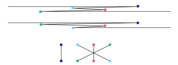
Figure 9. Another example of a pair of paths with a nontrivial collision partition and such that neither $\omega$ nor $\omega^{\prime}$ has a recollision event. The paths are depicted with a slight downward drift to clarify the order of the collisions. Note that this behavior is typical in one dimension.

This partition has a nontrivial structure because the second collision of $\omega^{-}$ correlates with the fourth collision of $\omega^{+}$ and vice-versa. This behavior is not uncommon for paths that are constrained to one dimension. The problem with the above example is that there are non-consecutive collisions in $\Gamma$ which can be visited by a single path with two collisions.

We need to introduce another type of incidence to prevent this behavior which we call a tube incidence.

Definition 4.6 (Tube incidences).

A tube incidence for a path $\omega\in\Omega_{\alpha,k}(s,S)$ is a pair $(a,a^{\prime})\in[0,k]$ of collisions such that there exists a collision $b\in I^{imm}(\omega)$ with $a<b<a^{\prime}$ and there exists a time $s\in{\mathbf{R}}$ such that

(4.8) $$|y_{a}+sp_{a}-y_{a^{\prime}}|\leq 100k^{4}\alpha^{20}r.$$

Above we use the convention $y_{0}=y_{1}-s_{0}p_{0}$. We set $I^{tube}(\omega)$ to be the set of pairs $(a,a^{\prime})$ that form a tube incidence.

A tube incidence occurs when a particle scattering out of site $a$ can choose to “skip” its next collision (possibly at $b$) and instead scatter at site $a^{\prime}$.

The key idea is that the partition $P({\mathbf{y}})$ of a doubled path $\bm{\Gamma}$ is severely constrained when neither $\omega^{+}$ nor $\omega^{-}$ have an incidence. In particular, the partition must be a generalized ladder. To define a generalized ladder we first define a ladder partition.

Definition 4.7 (Ladder partitions).

Let $A$ and $B$ be two finite ordered sets with $|A|=|B|$. The ladder matching $P_{lad}\in{\mathcal{P}}(A\sqcup B)$ is the unique matching of the form $P_{lad}=\{\{a,\varphi(a)\}\}_{a\in A}$ where $\varphi:A\to B$ is the unique order-preserving bijection between $A$ and $B$.

We can now state the main result.

Lemma 4.8.

Let $\bm{\Gamma}=(\xi_{0}^{+},\omega^{+},\xi_{1}^{+};\xi_{0}^{-},\omega^{-},\xi_{1}^{-})$ be a doubled path such that $X(\bm{\Gamma})$ is $|\log{\varepsilon}|^{20}$-complete and $d_{r}(\xi_{0}^{+},\xi_{0}^{-})\leq|\log{\varepsilon}|^{20}$. Then at least one of the following holds:

• One of $\omega^{+}$ or $\omega^{-}$ has an incidence. That is,

  $$I^{rec}(\omega^{+})\cup I^{tube}(\omega^{+})\cup I^{rec}(\omega^{-})\cup I^{tube}(\omega^{-})\not=\varnothing.$$

• The partition $P(\bm{\Gamma})$ has a cell with more than two elements.

• The partition $P(\bm{\Gamma})$ is a generalized ladder in the sense that (1) $P$ saturates the set $I^{imm}(\omega^{+})\cup I^{imm}(\omega^{-})$ and (2) The restriction $P|_{K(\bm{\Gamma})\setminus I^{imm}(\omega^{+})\setminus I^{imm}(\omega^{-})}$ is a ladder partition on the set $K(\Gamma^{+})\setminus I^{imm}(\omega^{+})\sqcup K(\Gamma^{-})\setminus I^{imm}(\omega^{-})$.

Proof.

We will assume that we are not in either of the first two cases, so that $P(\bm{\Gamma})$ is a perfect matching of $K(\bm{\Gamma})$ and neither $\omega^{+}$ nor $\omega^{-}$ has an incidence.

First we observe that every immediate recollision $(a,a+1)$ must also be a cell in $P(\bm{\Gamma})$. Since $P(\bm{\Gamma})$ is assumed to be a perfect matching, it follows that $P(\bm{\Gamma})$ saturates the set of immediate recollisions.

It remains to show that $P|_{K(\bm{\Gamma})\setminus I^{imm}(\bm{\Gamma})}$ forms a ladder partition. Order the collisions in $K(\Gamma^{+})\setminus I^{imm}(\Gamma^{+})$ as $(a_{1},a_{2},\cdots,a_{m})$, and the collisions of $K(\Gamma^{-})\setminus I^{imm}$ as $(b_{1},b_{2},\cdots,b_{m^{\prime}})$ (with $b_{j+1}>b_{j}$ and $a_{j+1}>a_{j}$).We first observe that there are no pairs $\{a_{j},a_{j^{\prime}}\}\in P(\bm{\Gamma})$ because then $(j,j^{\prime})$ would form a recollision. Likewise $\{b_{j},b_{j^{\prime}}\}\not\in P(\bm{\Gamma})$ for any $j,j^{\prime}$. This shows that $m=m^{\prime}$. To show that $P(\bm{\Gamma})$ is a generalized ladder, it suffices to check that $\{a_{j},b_{j}\}\in P(\bm{\Gamma})$ for every $j\in[m]$. We prove this by induction on $j$.

The base case is that $j=1$. Choose $j_{1}$ such that $\{a_{1},b_{j_{1}}\}\in P(\bm{\Gamma})$. then $|y_{a_{1}}-y_{b_{j_{1}}}|\leq 2r$. Using (4.7), we have

$$|y_{a_{1}}-(y_{+,0}+t_{a_{1}}p_{+,0})| \leq 4k^{2}\alpha^{20}r$$

$$|y_{b_{1}}-(y_{-,0}+t_{b_{1}}p_{-,0})| \leq 4k^{2}\alpha^{20}r.$$

It follows that for $s=t_{a_{1}}-t_{b_{1}}$,

$$|y_{b_{j_{1}}}-(y_{+,0}+sp_{-,0}|\leq 10k^{2}\alpha^{20}r,$$

so that either $j_{1}=1$ or else $j_{1}>1$ and therefore $(0,b_{j_{1}})$ is a tube incidence for $\Gamma^{-}$.

The proof of the inductive step follows the same argument, with an additional calculation to show that $|p_{a_{j}}-p_{b_{j}}|\leq m|\log{\varepsilon}|^{20}r^{-1}$ if $\{a_{j^{\prime}},b_{j^{\prime}}\}\in P(\bm{\Gamma})$ for all $j^{\prime}\leq j$. ∎

4.3. Ladders and the semigroup property

Now we state the main result of the section, which is that the expectation appearing in ${\mathcal{E}}_{s}[A]$ is well approximated by simply summing over the ladder matchings.

Definition 4.9 (Generalized ladders).

A generalized ladder partition on the set $[k_{+}]\sqcup[k_{-}]\{(\pm,j)\mid j\leq k_{\pm}\}$ is a partition $P$ of $[k_{+}]\sqcup[k_{-}]$ such that there exists a set $I_{+}^{imm}\subset[k_{+}]$ and $I_{-}^{imm}\subset[k_{-}]$ such that $\{(+,j),(+,j+1)\}\in P$ for every $j\in I_{+}^{\operatorname{Imm}}$ and $\{(-,j),(-,j+1)\}\in P$ for every $j\in I_{-}^{\operatorname{Imm}}$, and such that $P|_{[k_{+}]\sqcup[k_{-}]\setminus\{+\}\times I_{+}^{\operatorname{Imm}}\setminus\{-\}\times I_{-}^{\operatorname{Imm}}}$ is a ladder partition on the set $([k_{+}]\setminus I_{+}^{imm})\sqcup([k_{-}]\setminus I_{-}^{imm})$.

We set ${\mathcal{Q}}_{gl}\subset{\mathcal{P}}([k_{+}]\sqcup[k_{-}])$ to be the set of generalized ladder partitions.

To relate partitions to the superoperator ${\mathcal{E}}_{s}$ we first define the notion of a $P$-expectation. Given a partition $P\in{\mathcal{P}}([k_{+}]\sqcup[k_{-}])$, $\omega^{+}\in\Omega_{k_{+}}$ and $\omega^{-}\in\Omega_{k_{-}}$, we define

(4.9) $${\mathbf{E}\,}_{P}\begin{smallmatrix}\mathinner{\langle{\xi_{1}^{+}|O_{\omega^{+}}|\xi_{0}^{+}}\rangle}\\ \mathinner{\langle{\xi_{1}^{-}|O_{\omega^{-}}|\xi_{0}^{-}}\rangle}^{*}\end{smallmatrix}=\begin{smallmatrix}\mathinner{\langle{\xi_{1}^{+}|p_{+,k_{+}}}\rangle}\mathinner{\langle{p_{+,0}|\xi_{0}^{+}}\rangle}\\ \mathinner{\langle{\xi_{1}^{-}|p_{-,k_{-}}}\rangle}\mathinner{\langle{p_{-,0}|\xi_{0}^{-}}\rangle}\end{smallmatrix}e^{i(\varphi(\omega^{+})-\varphi(\omega^{-}))}{\varepsilon}^{k_{+}+k_{-}}\prod_{S\in P}{\mathbf{E}\,}\prod_{a\in S}{\widehat{V_{y_{a}}}}(q_{a}).$$

We then define the ladder expectation to be the sum over all ladder partitions,

$${\mathbf{E}\,}_{lad}\begin{smallmatrix}\mathinner{\langle{\xi_{1}^{+}|O_{\omega^{+}}|\xi_{0}^{+}}\rangle}\\ \mathinner{\langle{\xi_{1}^{-}|O_{\omega^{-}}|\xi_{0}^{-}}\rangle}^{*}\end{smallmatrix}:=\sum_{P\in{\mathcal{Q}}_{rl}([k_{+}]\sqcup[k_{-}])}{\mathbf{E}\,}_{P}\begin{smallmatrix}\mathinner{\langle{\xi_{1}^{+}|O_{\omega^{+}}|\xi_{0}^{+}}\rangle}\\ \mathinner{\langle{\xi_{1}^{-}|O_{\omega^{-}}|\xi_{0}^{-}}\rangle}^{*}\end{smallmatrix}$$

We are now ready to define the ladder superoperator ${\mathcal{L}}_{s}$.

(4.10) $${\mathcal{L}}_{s}[A]:=\int\mathinner{|{\xi_{0}^{-}}\rangle}\mathinner{\langle{\xi_{0}^{+}}|}\mathinner{\langle{\xi_{1}^{-}|A|\xi_{1}^{+}}\rangle}\Xi(\Gamma){\mathbf{E}\,}_{lad}\begin{smallmatrix}\mathinner{\langle{\xi_{1}^{+}|O_{\omega^{+}}|\xi_{0}^{+}}\rangle}\\ \mathinner{\langle{\xi_{1}^{-}|O_{\omega^{-}}|\xi_{0}^{-}}\rangle}^{*}\end{smallmatrix}\mathop{}\!\mathrm{d}\Gamma.$$

For convenience we define

The main result of this section is that the ladder superoperator ${\mathcal{L}}_{s}$ is a good approximation to the evolution ${\mathcal{E}}_{s}$.

Proposition 4.10.

Let $A$ be an operator with good support and let $s\leq{\varepsilon}^{-2-\kappa/2}$. Then

$$\|{\mathcal{E}}_{s}[A]-{\mathcal{L}}_{s}[A]\|_{op}\leq C{\varepsilon}^{2.1}s\|A\|_{op}.$$

Before we are ready to prove Proposition 4.10 we must first establish that the sum over all generalized ladders is the same as the sum over ther correct generalized ladder in the case that $\bm{\Gamma}$ is a path with no incidences.

Lemma 4.11.

Let $\bm{\Gamma}$ be a $|\log{\varepsilon}|^{20}$-complete path and suppose that $d_{r}(\xi_{0}^{+},\xi_{0}^{-})\leq|\log{\varepsilon}^{-20}$, and $|\xi_{p}|\geq r^{-1}\sigma^{-1}$. Suppose moreover that $\bm{\Gamma}$ has no incidences and that $P(\bm{\Gamma})$ is a matching. Then

$${\mathbf{E}\,}\begin{smallmatrix}\mathinner{\langle{\xi_{1}^{+}|O_{\omega^{+}}|\xi_{0}^{+}}\rangle}\\ \mathinner{\langle{\xi_{1}^{-}|O_{\omega^{-}}|\xi_{0}^{-}}\rangle}^{*}\end{smallmatrix}={\mathbf{E}\,}_{lad}\begin{smallmatrix}\mathinner{\langle{\xi_{1}^{+}|O_{\omega^{+}}|\xi_{0}^{+}}\rangle}\\ \mathinner{\langle{\xi_{1}^{-}|O_{\omega^{-}}|\xi_{0}^{-}}\rangle}^{*}\end{smallmatrix}.$$

Proof.

By Lemma 4.8, it follows that for some generalized ladder $P\in{\mathcal{Q}}_{gl}([k_{+}]\sqcup[k_{-}])$,

$${\mathbf{E}\,}\begin{smallmatrix}\mathinner{\langle{\xi_{1}^{+}|O_{\omega^{+}}|\xi_{0}^{+}}\rangle}\\ \mathinner{\langle{\xi_{1}^{-}|O_{\omega^{-}}|\xi_{0}^{-}}\rangle}^{*}\end{smallmatrix}={\mathbf{E}\,}_{P}\begin{smallmatrix}\mathinner{\langle{\xi_{1}^{+}|O_{\omega^{+}}|\xi_{0}^{+}}\rangle}\\ \mathinner{\langle{\xi_{1}^{-}|O_{\omega^{-}}|\xi_{0}^{-}}\rangle}^{*}\end{smallmatrix}.$$

We will show that if $P^{\prime}\in{\mathcal{Q}}_{gl}([k_{+}]\sqcup[k_{-}])$ is another generalized ladder with $P^{\prime}\not=P$, then

$${\mathbf{E}\,}_{P^{\prime}}\begin{smallmatrix}\mathinner{\langle{\xi_{1}^{+}|O_{\omega^{+}}|\xi_{0}^{+}}\rangle}\\ \mathinner{\langle{\xi_{1}^{-}|O_{\omega^{-}}|\xi_{0}^{-}}\rangle}^{*}\end{smallmatrix}=\prod_{S\in P}{\mathbf{E}\,}\prod_{a\in S}{\widehat{V_{y_{a}}}}(q_{a})=0.$$

Indeed, since $P^{\prime}\not=P$ there exists some $a,b,b^{\prime}\in[k_{+}]\sqcup[k_{-}]$ such that $\{a,b\}\in P=P(\bm{\Gamma})$ and $\{a,b^{\prime}\}\in P^{\prime}$ with $b\not=b$. But since $\{a,b^{\prime}\}\not\in P(\bm{\Gamma})$, $|y_{a}-y_{b^{\prime}}|>2r$ so the expectation

$${\mathbf{E}\,}{\widehat{V_{y_{a}}}}(q_{a}){\widehat{V_{y_{b}}}}(q_{b^{\prime}})=0$$

vanishes. ∎

4.4. The proof of Proposition 4.10

The error ${\mathcal{E}}_{s}[A]-{\mathcal{L}}_{s}[A]$ can be written as a path integral

$${\mathcal{E}}_{s}[A]-{\mathcal{L}}_{s}[A]=\int\mathinner{|{\xi_{0}^{-}}\rangle}\mathinner{\langle{\xi_{0}^{+}}|}\mathinner{\langle{\xi_{1}^{-}|A|\xi_{1}^{+}}\rangle}\Xi(\Gamma)\big{(}{\mathbf{E}\,}\begin{smallmatrix}\mathinner{\langle{\xi_{1}^{+}|O_{\omega^{+}}|\xi_{0}^{+}}\rangle}\\ \mathinner{\langle{\xi_{1}^{-}|O_{\omega^{-}}|\xi_{0}^{-}}\rangle}^{*}\end{smallmatrix}-{\mathbf{E}\,}_{lad}\begin{smallmatrix}\mathinner{\langle{\xi_{1}^{+}|O_{\omega^{+}}|\xi_{0}^{+}}\rangle}\\ \mathinner{\langle{\xi_{1}^{-}|O_{\omega^{-}}|\xi_{0}^{-}}\rangle}^{*}\end{smallmatrix}\big{)}\mathop{}\!\mathrm{d}\bm{\Gamma}.$$

The argument of Lemma 4.2 still works to show that we can restrict the integral to paths that are $|\log{\varepsilon}|^{20}$-complete. Moreover, using the support condition on $A$ we can also restrict to the case that $d_{r}(\xi_{1}^{+},\xi_{1}^{-})\leq|\log{\varepsilon}|^{20}$ and that $|(\xi_{1}^{+})_{p}|\geq(r\sigma)^{-1}$.

Under these constraints, the only paths that contribute to the path integral above are those for which either $P(\bm{\Gamma})$ has a cell of more than two elements and paths which have some kind of incidence. Let ${\mathbf{1}}^{bad}(\bm{\Gamma})$ be the indicator function for such paths. We decompose this function according to the exact partition $P(\bm{\Gamma})$ and the exact incidence set $I^{rec}(\bm{\Gamma})$, $I^{tube}(\bm{\Gamma})$,

$${\mathbf{1}}^{bad}(\bm{\Gamma}) =\sum_{P\in{\mathcal{P}}([k_{+}]\sqcup[k_{-}])}\sum_{I^{rec},I^{tube}}{\mathbf{1}}(P(\bm{\Gamma})=P){\mathbf{1}}(I^{rec}(\bm{\Gamma})=I^{rec}){\mathbf{1}}(I^{tube}(\bm{\Gamma})=I^{tube})$$

$$=:\sum_{P\in{\mathcal{P}}([k_{+}]\sqcup[k_{-}])}\sum_{I^{rec},I^{tube}}{\mathbf{1}}_{P,I^{rec},I^{tube}}(\bm{\Gamma}).$$

where the sum includes the constraint that either $I^{rec}\cup I^{rec}\not=\varnothing$ or else $P$ has a cell with at least three elements. Then we have the estimate

$$\|{\mathcal{E}}_{s}[A]-{\mathcal{L}}_{s}[A]\|_{op}\leq\sum_{P,I^{rec},I^{tube}}\Big{\|}\int\mathinner{|{\xi_{0}^{-}}\rangle}\mathinner{\langle{\xi_{0}^{+}}|} \mathinner{\langle{\xi_{1}^{-}|A|\xi_{1}^{+}}\rangle}\Xi(\Gamma){\mathbf{1}}_{P,I^{rec},I^{tube}}(\bm{\Gamma})$$

$$\big{(}{\mathbf{E}\,}\begin{smallmatrix}\mathinner{\langle{\xi_{1}^{+}|O_{\omega^{+}}|\xi_{0}^{+}}\rangle}\\ \mathinner{\langle{\xi_{1}^{-}|O_{\omega^{-}}|\xi_{0}^{-}}\rangle}^{*}\end{smallmatrix}-{\mathbf{E}\,}_{lad}\begin{smallmatrix}\mathinner{\langle{\xi_{1}^{+}|O_{\omega^{+}}|\xi_{0}^{+}}\rangle}\\ \mathinner{\langle{\xi_{1}^{-}|O_{\omega^{-}}|\xi_{0}^{-}}\rangle}^{*}\end{smallmatrix}\big{)}\mathop{}\!\mathrm{d}\bm{\Gamma}\Big{\|}_{op}.$$

Using the triangle inequality we bound

$$\big{|}{\mathbf{E}\,}\begin{smallmatrix}\mathinner{\langle{\xi_{1}^{+}|O_{\omega^{+}}|\xi_{0}^{+}}\rangle}\\ \mathinner{\langle{\xi_{1}^{-}|O_{\omega^{-}}|\xi_{0}^{-}}\rangle}^{*}\end{smallmatrix}-{\mathbf{E}\,}_{lad}\begin{smallmatrix}\mathinner{\langle{\xi_{1}^{+}|O_{\omega^{+}}|\xi_{0}^{+}}\rangle}\\ \mathinner{\langle{\xi_{1}^{-}|O_{\omega^{-}}|\xi_{0}^{-}}\rangle}^{*}\end{smallmatrix}\big{|}\leq\sum_{Q\leq P(\bm{\Gamma})}\big{|}{\mathbf{E}\,}_{Q}\begin{smallmatrix}\mathinner{\langle{\xi_{1}^{+}|O_{\omega^{+}}|\xi_{0}^{+}}\rangle}\\ \mathinner{\langle{\xi_{1}^{-}|O_{\omega^{-}}|\xi_{0}^{-}}\rangle}^{*}\end{smallmatrix}\big{|},$$

and now applying the Schur test we estimate

(4.11) $$\begin{split}\|{\mathcal{E}}_{s}[A]-{\mathcal{L}}_{s}[A]\|_{op}\leq\sum_{k_{+},k_{-}}&\sum_{P,I^{rec},I^{tube}}\\ &\sup_{\xi_{0}^{-}}\Big{|}\int\mathinner{\langle{\xi_{1}^{-}|A|\xi_{1}^{+}}\rangle}\Xi(\Gamma){\mathbf{1}}_{P,I^{rec},I^{tube}}(\bm{\Gamma})\sum_{Q\leq P(\bm{\Gamma})}|{\mathbf{E}\,}_{Q}\begin{smallmatrix}\mathinner{\langle{\xi_{1}^{+}|O_{\omega^{+}}|\xi_{0}^{+}}\rangle}\\ \mathinner{\langle{\xi_{1}^{-}|O_{\omega^{-}}|\xi_{0}^{-}}\rangle}^{*}\end{smallmatrix}|\mathop{}\!\mathrm{d}\omega^{\pm}\mathop{}\!\mathrm{d}\xi_{1}^{\pm}\mathop{}\!\mathrm{d}\xi_{0}^{-}\Big{|}^{1/2}\\ &\times\sup_{\xi_{0}^{+}}\Big{|}\int\mathinner{\langle{\xi_{1}^{-}|A|\xi_{1}^{+}}\rangle}\Xi(\Gamma){\mathbf{1}}_{P,I^{rec},I^{tube}}(\bm{\Gamma})\sum_{Q\leq P(\bm{\Gamma})}|{\mathbf{E}\,}_{Q}\begin{smallmatrix}\mathinner{\langle{\xi_{1}^{+}|O_{\omega^{+}}|\xi_{0}^{+}}\rangle}\\ \mathinner{\langle{\xi_{1}^{-}|O_{\omega^{-}}|\xi_{0}^{-}}\rangle}^{*}\end{smallmatrix}|\mathop{}\!\mathrm{d}\omega^{\pm}\mathop{}\!\mathrm{d}\xi_{1}^{\pm}\mathop{}\!\mathrm{d}\xi_{0}^{+}\Big{|}^{1/2}.\end{split}$$

The first step to bound the term ${\mathbf{E}\,}_{Q}\begin{smallmatrix}\mathinner{\langle{\xi_{1}^{+}|O_{\omega^{+}}|\xi_{0}^{+}}\rangle}\\ \mathinner{\langle{\xi_{1}^{-}|O_{\omega^{-}}|\xi_{0}^{-}}\rangle}^{*}\end{smallmatrix}$ appearing in the integrand. Then, expanding out the formula (4.9) we have

$$\big{|}{\mathbf{E}\,}_{Q}\begin{smallmatrix}\mathinner{\langle{\xi_{1}^{+}|O_{\omega^{+}}|\xi_{0}^{+}}\rangle}\\ \mathinner{\langle{\xi_{1}^{-}|O_{\omega^{-}}|\xi_{0}^{-}}\rangle}^{*}\end{smallmatrix}\big{|}\leq\begin{smallmatrix}|\mathinner{\langle{\xi_{1}^{+}|p_{+,k_{+}}}\rangle}\mathinner{\langle{p_{+,0}|\xi_{0}^{+}}\rangle}|\\ |\mathinner{\langle{\xi_{1}^{-}|p_{-,k_{-}}}\rangle}\mathinner{\langle{p_{-,0}|\xi_{0}^{-}}\rangle}|\end{smallmatrix}e^{i(\varphi(\omega^{+})-\varphi(\omega^{-}))}\prod_{S\in P(\bm{\Gamma})\vee Q}{\mathbf{E}\,}\prod_{a\in S}{\widehat{V_{y_{a}}}}(q_{a}).$$

Now we use

$$|\langle{p|\xi}\rangle|\leq Cr^{d/2}\exp(-c(r|(\xi)_{p}-p|)^{0.5})$$

as well as Lemma B.3 to estimate

$$\big{|}{\mathbf{E}\,}_{Q}\begin{smallmatrix}\mathinner{\langle{\xi_{1}^{+}|O_{\omega^{+}}|\xi_{0}^{+}}\rangle}\\ \mathinner{\langle{\xi_{1}^{-}|O_{\omega^{-}}|\xi_{0}^{-}}\rangle}^{*}\end{smallmatrix}\big{|}\leq Cr^{2d}{\varepsilon}^{k_{+}+k_{-}} \begin{smallmatrix}\exp(-c(r|(\xi_{1}^{+})_{p}-p_{+,k_{+}}|)^{0.5})\exp(-c(r|(\xi_{0}^{+})_{p}-p_{+,0}|)^{0.5})\\ \exp(-c(r|(\xi_{1}^{-})_{p}-p_{-,k_{-}}|)^{0.5})\exp(-c(r|(\xi_{0}^{-})_{p}-p_{-,0}|)^{0.5})\end{smallmatrix}$$

$$r^{-d(k_{+}+k_{-})}(C(k_{+}+k_{-}))^{k_{+}+k_{-}}\prod_{Q^{\prime}\leq P(\bm{\Gamma})\vee Q}\prod_{S^{\prime}\in Q^{\prime}}r^{d}\exp\Big{(}-c\big{|}r|S|^{-1}\sum_{a\in S}q_{a}\big{|}^{0.99}\Big{)}$$

$$\qquad\qquad\qquad\qquad\times\prod_{a\in[k_{+}]\sqcup[k_{-}]}(1+|q_{a}|)^{-20d}.$$

We collect the important terms above in the function $E_{Q}(\bm{\Gamma})$,

(4.12) $$E_{Q}(\bm{\Gamma}):=r^{2d}r^{-d(k_{+}+k_{-})}{\varepsilon}^{k_{+}+k_{-}}\prod_{S\in Q}r^{d}\exp(-c|\frac{r}{|S|}\sum_{a\in S}q_{a}|^{0.99})\times\prod_{a}(1+|q_{a}|)^{-20d}.$$

Because $k_{+},k_{-}\leq k_{max}$, the combinatorial factors contribute at most an absolute constant. Therefore Proposition 4.10 reduces to the following integral bound.

Lemma 4.12.

Let $A$ be an admissible operator, let $k_{+},k_{-}\in[k_{max}]$, let $Q\in{\mathcal{P}}([k_{+}]\sqcup[k_{-}])$, and let $(P,I^{rec},I^{imm})$ be a triple such that if $I^{rec}\cup I^{tube}=\varnothing$, then $P$ has a cell of more than two elements. Then

(4.13) $$\sup_{\xi_{0}^{-}}\Big{|}\int\mathinner{\langle{\xi_{1}^{-}|A|\xi_{1}^{+}}\rangle}\Xi(\Gamma)E_{Q\vee P}(\bm{\Gamma}){\mathbf{1}}_{P,I^{rec},I^{tube}}(\bm{\Gamma})\mathop{}\!\mathrm{d}\omega^{\pm}\mathop{}\!\mathrm{d}\xi_{1}^{\pm}\mathop{}\!\mathrm{d}\xi_{0}^{-}\Big{|}\leq C{\varepsilon}^{2.25}\tau.$$

To estimate (4.13) we use the following simple lemma, which is just an iterated application of Fubini’s theorem and the triangle inequality.

Lemma 4.13.

Let ${\mathcal{X}}=X_{1}\times\cdots\times X_{N}$ be the product of $N$ measure spaces $X_{j}$, and let ${\mathcal{X}}_{j}=X_{1}\times\cdots\times X_{j}$ be the product of the first $j$ factors. Then for any positive functions $F_{j}:{\mathcal{X}}_{j}\to{\mathbf{R}}^{+}$,

(4.14) $$\int_{{\mathcal{X}}}\prod_{j=1}^{N}F_{j}(x_{1},\cdots,x_{j})\mathop{}\!\mathrm{d}X\leq\prod_{j=1}^{N}\sup_{x^{\prime}_{1},\dots,x^{\prime}_{j-1}}\int_{X_{j}}F_{j}(x^{\prime}_{1},\dots,x^{\prime}_{j-1},x_{j})\mathop{}\!\mathrm{d}x_{j}.$$

To apply Lemma 4.13 we need to order the variables in $\bm{\Gamma}$ and bound the integrand as a product of functions constraining each variable in $\bm{\Gamma}$ as a function only of variables that come earlier in the ordering. The reader may find it useful to refer to Figure 10 for a quick overview of the constraints on the variables.

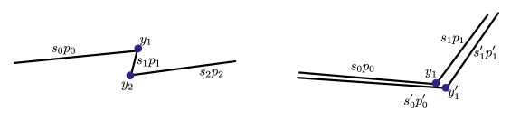
Figure 10. Two typical collision pairs that can appear. On the left, a recollision. The contribution from recollisions is heuristically counted as follows: The $s_{0}$ variable has only the constraint $0\leq s_{0}\leq\tau$. The $s_{1}$ variable is then constrained to $s_{1}{\,\lesssim\,}r|p_{1}|^{-1}$ so that $|y_{1}-y_{2}|\leq r$. Then $p_{1}$ is chosen from an annulus of width $r^{-1}$ and radius $|p_{0}|$ and $p_{2}$ is effectively constrained by a delta function in the momentum variables. The total contribution is at most ${\varepsilon}^{2}\tau{\,\lesssim\,}1$. On the right, a typical “rung” collision forming a ladder. The time variable $s_{0}$ satisfies $0\leq s_{0}\leq\tau$, but then $s_{0}^{\prime}$ is constrained by $|s_{0}-s^{\prime}_{0}|{\,\lesssim\,}r|p_{0}|^{-1}$ so that $|y_{1}-y_{1}^{\prime}|\leq r$. The momentum variable $p_{1}$ is again chosen from an annulus of thickness $r^{-1}$ and width $|p_{0}|$, and $p_{1}^{\prime}$ is constrained by a delta function to match $p_{1}$. Again the contribution is bounded by ${\varepsilon}^{2}\tau$.

We use the following ordering of the variables:

(4.15) $$\bm{\Gamma}=(\xi_{0}^{+},p_{+,0},s_{+,0},y_{+,1},\cdots,y_{+,k_{+}},p_{+,k_{+}},s_{+,k_{+}},\xi_{1}^{+},\xi_{1}^{-},p_{-,k_{-}},s_{-,k_{-}},y_{-,k_{-}},\cdots,y_{-,1}p_{-,0},s_{-,0},\xi_{0}^{-}).$$

Given a variable label $\lambda\in\{{\mlq\mlq y\mrq\mrq}_{a},{\mlq\mlq p\mrq\mrq}_{a},{\mlq\mlq s\mrq\mrq}_{a}\}_{a\in K(\bm{\Gamma})}\cup\{{\mlq\mlq\xi\mrq\mrq}_{\ell}^{\pm}\}_{\ell\in\{0,1\}}$, we define the partial paths $\bm{\Gamma}_{<\lambda}$ to be the sequence of variables preceding $\lambda$. Thus for example $\bm{\Gamma}_{<{\mlq\mlq y\mrq\mrq}_{+,1}}=(\xi_{0}^{+},p_{+,0},s_{+,0})$. We also define a total ordering $\leq^{\prime}$ on $[k_{+}]\sqcup[k_{-}]$ implied by the ordering of the variables (14.3), in which $(+,j)\leq^{\prime}(-,j^{\prime})$ for any $j,j^{\prime}$ and $(\pm,j)\leq(\pm,j^{\prime})$ when $\pm j\leq\pm j^{\prime}$ (that is, the ordering is reversed for the negative indices, as indicated in (14.3)).

The next step is to bound the integrand as a product of constraints assigned to each variable as a function of the prior variables. ${\mathbf{1}}_{P,I^{rec},I^{tube}}(\bm{\Gamma})$. We will write out the “standard term” in the integrand that does not use the indicator function as a product of constraints of the $p$, $y$, and $\xi$ variables.

$$|\mathinner{\langle{\xi_{1}^{-}|A|\xi_{1}^{+}}\rangle}||\Xi(\bm{\Gamma})|E_{Q\vee P}(\bm{\Gamma})\leq{\varepsilon}^{k_{+}+k_{-}}F_{p}(\bm{\Gamma})F_{y}(\bm{\Gamma})F_{\xi}(\bm{\Gamma}).$$

The constraints on momentum come from several sources. First there is a term $\prod(1+|q_{a}|)^{-20d}$ ensuring that no impulse is too large. Second, there is a term enforcing conservation of kinetic energy. Third, there are terms ensuring that $p_{+,0}$ and $p_{-,k_{-}}$ match with $(\xi_{0}^{+})_{p}$ and $(\xi_{1}^{-})_{p}$, respectively. Finally, there are the constraints (approximate delta functions) coming from the expectation. We also take the factor of $r^{2d}$ from (4.12) and distribute one factor of $r^{d}$ to each $p_{+,0}$ and $p_{-,k_{-}}$:

$$F_{p}(\bm{\Gamma}):= \prod(1+|p_{a}-p_{a-1}|)^{-20d}\prod{\mathbf{1}}(||p_{\pm,j}|-|p_{\pm,0}||\leq\alpha\max\{s_{\pm,j}^{-1},r^{-1}\})$$

$$\times(r^{d}{\mathbf{1}}(|p_{+,0}-(\xi_{0}^{+})_{p}|\leq\alpha r^{-1}))(r^{d}{\mathbf{1}}(|p_{-,{k_{-}}}-(\xi_{1}^{-})_{p}|\leq\alpha r^{-1}))\prod_{S\in{Q\vee P}}r^{d}\exp(-ck_{max}^{-1}|r\sum_{a\in S}q_{a}|^{0.99})$$

The constraints in the position variables are determined by the compatibility conditions $|y_{a+1}-(y_{a}+s_{a}p_{a})|\leq\alpha r$ and the compatibility of the first and last collisions of $\omega^{+}$ and $\omega^{-}$ against the boundaries $\xi_{0}^{+}$ and $\xi_{1}^{-}$. We take the factor of $r^{-d(k_{+}+k_{-})}$ from (4.12) and distribute one $r^{-d}$ to each $y_{a}$ variable:

$$F_{y}(\bm{\Gamma}):= \prod(r^{-d}{\mathbf{1}}(|y_{a+1}-(y_{a}+s_{a}p_{a})|\leq\alpha r))$$

$$\qquad\times(r^{-d}{\mathbf{1}}(|y_{+,1}-((\xi^{+}_{0})_{x}+s_{0}p_{0})|\leq\alpha r))(r^{-d}{\mathbf{1}}(|y_{-,k_{-}}-((\xi^{-}_{1})_{x}-s_{-,k_{-}}p_{-,k_{-}})|)).$$

The constraint on the $\xi$ variables comes from the compatibility with the path, along with the support condition on $A$

$$F_{\xi}(\bm{\Gamma}):={\mathbf{1}}(d_{r}(\xi_{1}^{+},(y_{+,k_{+}}+s_{+,k_{+}}p_{+,k_{+}},p_{+,k_{+}}))\leq\alpha){\mathbf{1}}(d_{r}(\xi_{0}^{-},(y_{-,1}-s_{-,0}p_{-,0},p_{-,0}))\leq\alpha)(1+d_{r}(\xi_{1}^{+},\xi_{1}^{-}))^{-20d}.$$

There are also indirect constraints on the $s$ variables coming indirectly from the combination of the compatibility conditions $|y_{a+1}-(y_{a}+s_{a}p_{a})|\leq\alpha r$ and constraints of the form $|y_{a}-y_{b}|\leq 2kr$ for collisions $a\sim_{P}b$ of the same cell of the partition $P(\bm{\Gamma})$. We also note that by Lemma 4.5, we have $|y_{a^{\prime}}-(y_{a}+(t_{a^{\prime}}-t_{a})p_{a})|\leq C\alpha^{20}r$ when $a$ and $a^{\prime}$ are collisions separated only by immediate recollisions.

We have no worry of “double-dipping” on the basic compatibility constraints such as ${\mathbf{1}}(|y_{a+1}-(y_{a}+s_{a}p_{a})|\leq\alpha r)$ because for example

$$\operatorname{supp}(F_{p}(\bm{\Gamma})F_{y}(\bm{\Gamma})F_{\xi}(\bm{\Gamma}))\subset\{|y_{a+1}-(y_{a}+s_{a}p_{a})|\leq\alpha r\},$$

so we can freely apply extra such indicator functions where they are useful.

4.4.1. The “standard constraint” bounds

In this section we use the partitions $P$ and $Q$ to “assign constraints” to each variable.

In particular, we write define functions $f_{\lambda}(\bm{\Gamma}_{\leq\lambda})$ such that

$$F_{p}(\bm{\Gamma}) \leq\prod f_{{\mlq\mlq p\mrq\mrq},a}(\bm{\Gamma}_{\leq{\mlq\mlq p\mrq\mrq},a})$$

$$F_{y}(\bm{\Gamma}) \leq\prod f_{{\mlq\mlq y\mrq\mrq},a}(\bm{\Gamma}_{\leq{\mlq\mlq y\mrq\mrq},a})$$

$$F_{\xi}(\bm{\Gamma}) \leq f_{{\mlq\mlq\xi\mrq\mrq},1,+}(\bm{\Gamma}_{\leq{\mlq\mlq\xi\mrq\mrq},1,+})f_{{\mlq\mlq\xi\mrq\mrq},1,-}(\bm{\Gamma}_{\leq{\mlq\mlq\xi\mrq\mrq},1,-})f_{{\mlq\mlq\xi\mrq\mrq},0,-}(\bm{\Gamma}_{\leq{\mlq\mlq\xi\mrq\mrq},0,-}).$$

These “standard constraint” functions can simply be read off of the definitions of $F_{p}$, $F_{y}$, and $F_{\xi}$.

(4.16) $$f_{{\mlq\mlq p\mrq\mrq},a}(\bm{\Gamma}_{\leq{\mlq\mlq p\mrq\mrq},a}):=\begin{cases}r^{d}\exp(-ck_{max}^{-1}|r\sum_{a\in S}q_{a}|^{0.99}),&a=\max_{\leq^{\prime}}S\text{ for some }S\in P\vee Q\\ r^{d}{\mathbf{1}}(|p_{-,k_{-}}-(\xi_{1}^{-})_{p}|\leq\alpha r^{-1}),&a=(-,k_{-})\\ r^{d}{\mathbf{1}}(|p_{+,0}-(\xi_{0}^{+})_{p}|\leq\alpha r^{-1}),&a=(+,0)\\ (1+|p_{a}-p_{a-1}|)^{-20d}{\mathbf{1}}(||p_{a}|-|p_{+,0}||\leq\alpha\max\{|p_{0}|^{-1}s_{a}^{-1},r^{-1}\}),&\text{ else}.\end{cases}$$

The standard $y$ constraints are given by

(4.17) $$f_{{\mlq\mlq y\mrq\mrq},a}(\bm{\Gamma}_{\leq{\mlq\mlq y\mrq\mrq},a}):=\begin{cases}r^{-d}{\mathbf{1}}(|y_{+,1}-((\xi^{+}_{0})_{x}+s_{0}p_{0})|\leq\alpha r),&a=(+,1)\\ r^{-d}{\mathbf{1}}(|y_{-,k_{-}}-((\xi^{-}_{1})_{x}-s_{-,k_{-}}p_{-,k_{-}})|),&a=(-,k_{-})\\ r^{-d}{\mathbf{1}}(|y_{+,j}-(y_{+,j-1}+s_{+,j-1}p_{+,j-1})|\leq\alpha r),&a=(+,j)\text{ for }j>1\\ r^{-d}{\mathbf{1}}(|y_{-,j+1}-(y_{-,j}+s_{-,j}p_{-,j})|\leq\alpha r),&a=(-,j)\text{ for }j<k_{-}.\end{cases}$$

Finally, the standard $\xi$ constraints are

$$f_{{\mlq\mlq\xi\mrq\mrq},1,+}(\bm{\Gamma}_{\leq{\mlq\mlq\xi\mrq\mrq},1,+}) :={\mathbf{1}}(d_{r}(\xi_{1}^{+},(y_{+,k_{+}}+s_{+,k_{+}}p_{+,k_{+}},p_{+,k_{+}}))\leq\alpha)$$

$$f_{{\mlq\mlq\xi\mrq\mrq},1,-}(\bm{\Gamma}_{\leq{\mlq\mlq\xi\mrq\mrq},1,-}) :=(1+d_{r}(\xi_{1}^{+},\xi_{1}^{-}))^{-20d}$$

$$f_{{\mlq\mlq\xi\mrq\mrq},0,-}(\bm{\Gamma}_{\leq{\mlq\mlq\xi\mrq\mrq},0,-}) :={\mathbf{1}}(d_{r}(\xi_{0}^{-},(y_{-,1}-s_{-,0}p_{-,0},p_{-,0}))\leq\alpha).$$

The contributions from the ${\mlq\mlq\xi\mrq\mrq}$ and ${\mlq\mlq y\mrq\mrq}$ variables are easy to account for

Lemma 4.14 (Standard position and phase space bounds).

For any $\lambda\in\{({\mlq\mlq y\mrq\mrq},a),({\mlq\mlq\xi\mrq\mrq},\ell,\pm)\}$

$$\sup_{\bm{\Gamma}_{<\lambda}}\int f_{\lambda}(\bm{\Gamma}_{\leq\lambda})\mathop{}\!\mathrm{d}\Gamma_{\lambda}\leq C.$$

The momentum constraints are slightly more complicated.

Lemma 4.15 (Standard momentum bounds).

If $a=\max_{\leq^{\prime}}S$ for some $S\in P\vee Q$ or $a\in\{(-,k_{-}),(+,0)\}$, then

$$\sup_{\bm{\Gamma}_{<{\mlq\mlq p\mrq\mrq},a}}\int f_{{\mlq\mlq p\mrq\mrq},a}(\bm{\Gamma}_{\leq{\mlq\mlq p\mrq\mrq},a})\mathop{}\!\mathrm{d}p_{a}\leq C.$$

Otherwise, if $a\not\sim_{P}a+1$ is not the first collision of an immediate recollision, then

(4.18) $$\sup_{\bm{\Gamma}_{<{\mlq\mlq p\mrq\mrq},a}}\int f_{{\mlq\mlq p\mrq\mrq},a}(\bm{\Gamma}_{\leq{\mlq\mlq p\mrq\mrq},a})\mathop{}\!\mathrm{d}p_{a}\leq Cr^{-1}\min\{|p_{0}|^{d-1},1\}.$$

Proof.

Only the second bound needs proof. Since $a+1\not\sim_{P}a$, it follows from Lemma 4.4 that $s_{a}\gtrsim\alpha|p_{0}|^{-1}r$. Therefore $|p_{0}|^{-1}s_{a}^{-1}{\,\lesssim\,}r^{-1}$, so $p_{a}$ is constrained to an annulus of thickness $r^{-1}$ and radius $|p_{0}|$. This annulus has volume $r^{-1}|p_{0}|^{d-1}$. If $|p_{0}|\gtrsim 1$ the additional factor $(1+|p_{a}-p_{a-1}|)^{-20d}$ ensures that $p_{a}$ is essentially also confined to a ball of unit radius. ∎

The immediate recollisions require some more detailed attention. If $a\sim a+1$ is an immediate recollision, then we group the variables $(s_{a},p_{a})$ and use the following estimate.

Lemma 4.16.

For any $|p_{0}|>r^{-1}\sigma^{-1}\geq{\varepsilon}^{0.5}$ and $q\in{\mathbf{R}}^{d}$,

(4.19) $$\begin{split}\int_{0}^{10\alpha|p_{0}|^{-1}r}\int_{{\mathbf{R}}^{d}}&{\mathbf{1}}(||p|^{2}/2-|p_{0}|^{2}/2|\leq\alpha s^{-1})(1+|p-q|)^{-20d}\mathop{}\!\mathrm{d}q\mathop{}\!\mathrm{d}s\\ &\leq C\min\{|p_{0}|^{-1},|p_{0}|^{d-2}\}(1+\log({\varepsilon}^{-1})).\end{split}$$

Proof.

We split the integral over $s$ into dyadic intervals $[2^{k},2^{k+1}]$ for $k\in{\mathbb{Z}}$. On this interval, the variable $p$ is retricted to an annulus of radius $|p_{0}|$ and width $|p_{0}|^{-1}2^{-k}$. Moreover,

Now consider the case $|p_{0}|\gtrsim 1$. In this case the factor $(1+|p-q|)^{-20d}$ additionally restricts the integration over $p$ to a unit ball, and the integration over $p_{0}$ produces a factor on the order $\min\{1,|p_{0}|^{-1}2^{-k}\}$. Integrating over $s$ to produce a factor $2^{k}$ and summing over $k$ such that $2^{k}\leq 20\alpha|p_{0}|^{-1}r$, we obtain the bound

$$\int_{0}^{10\alpha|p_{0}|^{-1}r}\int_{{\mathbf{R}}^{d}} {\mathbf{1}}(||p|^{2}/2-|p_{0}|^{2}/2|\leq\alpha s^{-1})(1+|p-q|)^{-20d}\mathop{}\!\mathrm{d}q\mathop{}\!\mathrm{d}s$$

$$\leq\sum_{\begin{subarray}{c}k\in{\mathbb{Z}}\\ 2^{k}<|p_{0}|^{-1}\end{subarray}}2^{k}+\sum_{\begin{subarray}{c}|p_{0}|^{-1}<2^{k}<20\alpha|p_{0}|^{-1}r\end{subarray}}|p_{0}|^{-1}$$

$$\leq|p_{0}|^{-1}(1+\log(20\alpha r)).$$

The second case we consider is that $|p_{0}|\lesssim 1$. In this case, the annulus of radius $|p_{0}|$ and width $|p_{0}|^{-1}2^{-k}$ has volume on the order $|p_{0}|^{d-2}2^{-k}$. The bound then follows from integrating in $s$ and summming over $k$, as above. ∎

Conspicuously missing from the discussion above is the integration over the time variables. For many of the time variables we simply use the constraint $s_{a}\leq\tau$ to pick up a factor of $\tau$. Additional constraints come from the partition $P$. Suppose that $a\leq^{\prime}b$ and $a\sim_{P}b$. Then there is a constraint $|y_{b}-y_{a}|\leq 2r$, which coupled with the constraint $|y_{b}-(y_{b-1}+s_{b-1}p_{b-1})|\leq\alpha r$ imposes a constraint on $s_{b-1}$ in terms of the variables $y_{a}$,$y_{b-1}$, and $p_{b-1}$, which are all in $\Gamma_{<{\mlq\mlq s\mrq\mrq},b}$. This constraint picks up a factor of $|p_{0}|^{-1}r$ instead of $\tau$:

(4.20) $$\sup_{\Gamma_{<{\mlq\mlq s\mrq\mrq},b-1}}\int{\mathbf{1}}(|y_{a}-(y_{b-1}+s_{b-1}p_{b-1})|\leq\alpha r)\mathop{}\!\mathrm{d}s_{b-1}\leq|p_{0}|^{-1}r.$$

4.4.2. The case that $P$ has a cluster

With just the bounds we have already proven, it is possible to obtain a good estimate in the case that $P$ has a set of more than $2$ elements. This is the simplest case, as suggested by Figure 11.

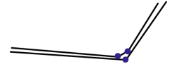
Figure 11. The case that the collision partition has a cluster. There is only one full time degree of freedom contributing a factor of $\tau$, but three factors of ${\varepsilon}$ from the potential. Such clusters therefore contribute ${\varepsilon}^{3}\tau$ rather than ${\varepsilon}^{2}\tau$.

Lemma 4.17 (The cluster bound).

Let $A$ be an admissible operator, let $k_{+},k_{-}\in[k_{max}]$, let $Q\in{\mathcal{P}}([k_{+}]\sqcup[k_{-}])$, and let $P\in{\mathcal{P}}([k_{+}]\sqcup[k_{-}])$ be a partition having a cell of more than two elements. Then

(4.21) $$\sup_{\xi_{0}^{-}}\Big{|}\int\mathinner{\langle{\xi_{1}^{-}|A|\xi_{1}^{+}}\rangle}\Xi(\Gamma)E_{Q\vee P}(\bm{\Gamma}){\mathbf{1}}_{P}(\bm{\Gamma})\mathop{}\!\mathrm{d}\omega^{\pm}\mathop{}\!\mathrm{d}\xi_{1}^{\pm}\mathop{}\!\mathrm{d}\xi_{0}^{-}\Big{|}\leq C^{k_{+}+k_{-}}({\varepsilon}^{2}\tau)^{(k_{+}+k_{-})/2}\tau^{-1}.$$

Proof.

We bound the standard part of the integrand by the product $F_{p}F_{y}F_{s}$ as described in the previous section and apply Lemma 4.13. The ${\mlq\mlq y\mrq\mrq}$ and ${\mlq\mlq\xi\mrq\mrq}$ variables contribute a factor of $C^{k_{+}+k_{-}}$. The product of the contributions from the $(s_{a},p_{a})$ pairs coming from immediate recollisions produces a factor of $(C\log{\varepsilon}^{-1})^{n_{r}}$, where $n_{r}$ is the number of immediate recollision clusters of $P$. To account for the ${\mlq\mlq s\mrq\mrq}$ and ${\mlq\mlq p\mrq\mrq}$ variables, let $P^{\prime}\subset P$ The ${\mlq\mlq p\mrq\mrq}$ variables contribute a total of $(Cr^{-1}\min\{|p_{0}|^{d-1},1\})^{|P|-n_{r}}$ by taking the product of the integral over all $p_{a}$ with $a=\max_{\leq^{\prime}}S$ for each $S\in P$. Then for each $s_{a}$ variable that is the first in its cluster (of which there are $|P|$), we get a trivial factor of $\tau$. Each of the rest of the $s_{a}$ variables contribute $|p_{0}|^{-1}r$ by (4.20). The product of all of these factors gives

(4.22) $$\begin{split}\sup_{\xi_{0}^{-}}\Big{|}&\int\mathinner{\langle{\xi_{1}^{-}|A|\xi_{1}^{+}}\rangle}\Xi(\Gamma)E_{Q\vee P}(\bm{\Gamma}){\mathbf{1}}_{P}(\bm{\Gamma})\mathop{}\!\mathrm{d}\omega^{\pm}\mathop{}\!\mathrm{d}\xi_{1}^{\pm}\mathop{}\!\mathrm{d}\xi_{0}^{-}\Big{|}\\ &\qquad\leq C^{k_{+}+k_{-}}{\varepsilon}^{k_{+}+k_{-}}\tau^{|P|}(C\min\{|p_{0}|^{d-2},|p_{0}|^{-1}\})^{|P|-n_{r}}\end{split}$$

The first and last factors are bounded by $C^{k_{+}+k_{-}}$. Then the fact that $P$ is not a perfect matching implies $|P|<(k_{+}+k_{-})/2$ and since $|P|$ is an integer in particular it follows that $|P|\leq(k_{+}+k_{-})/2-1$. This proves (4.21). ∎

4.4.3. The recollision case

To complete the proof of Lemma 4.12 we need to find a way to use the additional constraints coming from a recollision or tube incidence. A simplified version of the argument is presented in Figure 12

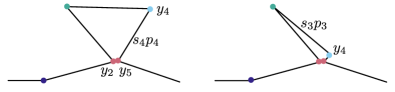
Figure 12. A path with a recollision at indices $(2,5)$. On the left, the case that $y_{4}$ is far from $y_{5}$. In this case the momentum variable $p_{4}$ is constrained to be approximately parallel to $y_{2}-y_{4}$. On the right, the case that $y_{4}$ is close to $y_{5}$. In this case there is an additional constraint on the time variable $s_{3}$.

Suppose that $(a,b)$ is a recollision occuring in $\omega^{+}$, $\operatorname{sgn}(a)=\operatorname{sgn}(b)=+$. The idea is that a recollision at $(a,b)$ typically enforces a strong constraint on the momentum before the collision at $b$. Indeed, if $|y_{a}-y_{b}|\leq 2r$ then $|s_{b-1}p_{b-1}-(y_{a}-y_{b-1})|\leq 2r$, so in particular

$$|p_{b-1}-z|\leq 2rs_{b-1}^{-1},$$

with $z=(y_{a}-y_{b-1})s_{b-1}^{-1}$. If $|y_{a}-y_{b-1}|>10\alpha r$, then $s_{b-1}\geq|y_{a}-y_{b-1}||p_{0}|^{-1}$. This is where the constraint on $p_{b-1}$ comes from. On the other hand, if $|y_{a}-y_{b-1}|$ is small, then there is a constraint on $s_{b-2}$ of exactly the same kind as (4.20). The only additional subtlety to deal with is the possibility that $b-1$ is itself a recollision or immediate recollision, in which case $p_{b-1}$ is localized by the momentum constraint on a collision cluster and further localization is not helpful. This is only a minor difficulty, and so we now prove

Lemma 4.18 (The recollision bound).

Let $A$ be an admissible operator, let $k_{+},k_{-}\in[k_{max}]$, let $P,Q\in{\mathcal{P}}([k_{+}]\sqcup[k_{-}])$, and let $I^{rec}\not=\varnothing$ be a nonempty set of recollisions in $[k_{+}]$. Then

(4.23) $$\sup_{\xi_{0}^{-}}\Big{|}\int\mathinner{\langle{\xi_{1}^{-}|A|\xi_{1}^{+}}\rangle}\Xi(\Gamma)E_{Q}(\bm{\Gamma}){\mathbf{1}}_{P}(\bm{\Gamma}){\mathbf{1}}_{I^{rec}}(\bm{\Gamma})\mathop{}\!\mathrm{d}\omega^{\pm}\mathop{}\!\mathrm{d}\xi_{1}^{\pm}\mathop{}\!\mathrm{d}\xi_{0}^{-}\Big{|}\leq C^{k_{+}+k_{-}}({\varepsilon}^{2}\tau)^{(k_{+}+k_{-})/2}({\varepsilon}^{-1.5}\tau^{-1}).$$

Proof.

Let $(a,a^{\prime})\in I^{rec}$ be the recollision with minimal $a^{\prime}$. Then let $b<a^{\prime}$ be the first collision before $a^{\prime}$ that is not an immediate recollision. Because $(a,a^{\prime})$ is not an immediate recollision, it is clear that $b\not=a^{\prime}$. Moreover, because $(a,a^{\prime})$ is minimal, the index $b$ is not of the form $\max_{\leq^{\prime}}S$ for any $S\in Q$.

We bound the indicator function for a recollision as a sum of indicator functions depending on the distance $|y_{b-1}-y_{b}|$

$${\mathbf{1}}_{I^{rec}}(\bm{\Gamma})\leq{\mathbf{1}}(|y_{a}-y_{b}|\leq 2r){\mathbf{1}}(|y_{b-1}-y_{b}|\geq Kr)+{\mathbf{1}}(|y_{b-1}-y_{b}|\leq Kr),$$

and use this to split (4.27) as a sum of two integrals each corresponding to a different term.

For the first term we follow the proof of Lemma 4.17, with the modification that we set

$$f^{\prime}_{{\mlq\mlq p\mrq\mrq},b-1}(\bm{\Gamma}_{\leq{\mlq\mlq p\mrq\mrq}_{b-1}})={\mathbf{1}}(|p_{b-1}-|p_{0}|\frac{y_{b-1}-y_{a}}{|y_{b-1}-y_{a}|}|\leq|p_{0}|K^{-1}).$$

In this case $p_{b-1}$ is sampled from the intersection of an annulus with thickness $r^{-1}$ and radius $|p_{0}|$ and a ball or radius $|p_{0}|K^{-1}$, so that

$$\sup_{\bm{\Gamma}_{<{\mlq\mlq p\mrq\mrq}_{b-1}}}\int f^{\prime}_{{\mlq\mlq p\mrq\mrq},b-1}(\bm{\Gamma}_{\leq{\mlq\mlq p\mrq\mrq}_{b-1}})\mathop{}\!\mathrm{d}p_{b-1}\leq Cr^{-1}\min\{(K^{-1}|p_{0}|)^{d-1},1\}.$$

Applying this estimate in the place of the bound (4.18) along with the rest of the argument that leads to (4.22) yields

(4.24) $$\begin{split}\sup_{\xi_{0}^{-}}\Big{|}&\int\mathinner{\langle{\xi_{1}^{-}|A|\xi_{1}^{+}}\rangle}\Xi(\Gamma)E_{Q\vee P}(\bm{\Gamma}){\mathbf{1}}_{P}(\bm{\Gamma}){\mathbf{1}}(|y_{a}-y_{b}|\leq 2r){\mathbf{1}}(|y_{b-1}-y_{b}|\geq Kr)\mathop{}\!\mathrm{d}\omega^{\pm}\mathop{}\!\mathrm{d}\xi_{1}^{\pm}\mathop{}\!\mathrm{d}\xi_{0}^{-}\Big{|}\\ &\qquad\leq C^{k_{+}+k_{-}}{\varepsilon}^{k_{+}+k_{-}}\tau^{|P|}(C\min\{|p_{0}|^{d-2},|p_{0}|^{-1}\})^{|P|-n_{r}-1}(C\min\{K^{1-d}|p_{0}|)^{d-2},|p_{0}|^{-1}\})\end{split}$$

The last factor is maximized when $|K^{1-d}||p_{0}|^{d-1}=|p_{0}|^{-1}$, which occurs when $|p_{0}|=K$. In this case we obtain a savings of $K^{-1}$ over the bound (4.22), and therefore conclude

(4.25) $$\begin{split}\sup_{\xi_{0}^{-}}\Big{|}&\int\mathinner{\langle{\xi_{1}^{-}|A|\xi_{1}^{+}}\rangle}\Xi(\Gamma)E_{Q\vee P}(\bm{\Gamma}){\mathbf{1}}_{P}(\bm{\Gamma}){\mathbf{1}}(|y_{a}-y_{b}|\leq 2r){\mathbf{1}}(|y_{b-1}-y_{b}|\geq Kr)\mathop{}\!\mathrm{d}\omega^{\pm}\mathop{}\!\mathrm{d}\xi_{1}^{\pm}\mathop{}\!\mathrm{d}\xi_{0}^{-}\Big{|}\\ &\qquad\leq C^{k_{+}+k_{-}}{\varepsilon}^{k_{+}+k_{-}}\tau^{|P|}K^{-1}.\end{split}$$

The second term to deal with is the integral involving ${\mathbf{1}}(|y_{b-1}-y_{b}|\leq Kr)$. In this case, we apply the bound (4.20) to get a factor of $Kr$ instead of $\tau$ for the integration over the variable $s_{b-2}$. Thus

(4.26) $$\begin{split}\sup_{\xi_{0}^{-}}\Big{|}&\int\mathinner{\langle{\xi_{1}^{-}|A|\xi_{1}^{+}}\rangle}\Xi(\Gamma)E_{Q\vee P}(\bm{\Gamma}){\mathbf{1}}_{P}(\bm{\Gamma}){\mathbf{1}}(|y_{b-1}-y_{b}|\leq Kr)\mathop{}\!\mathrm{d}\omega^{\pm}\mathop{}\!\mathrm{d}\xi_{1}^{\pm}\mathop{}\!\mathrm{d}\xi_{0}^{-}\Big{|}\\ &\qquad\leq C^{k_{+}+k_{-}}{\varepsilon}^{k_{+}+k_{-}}\tau^{|P|}(Kr\tau^{-1}).\end{split}$$

Choosing $K={\varepsilon}^{-0.5}$ yields the desired result. ∎

4.4.4. The tube incidence case

The final remaining case is that $\bm{\Gamma}$ does not have a recollision but does have a tube incidence. Suppose that the first tube incidence occurs at $(a,b)$. Then combining the tube incidence constraint (4.8) with the compatibility condition $|y_{b}-y_{b-1}-s_{b-1}p_{b-1}|\leq 2r$, we conclude that there exists $s\in{\mathbf{R}}$ such that

$$|s_{b-1}p_{b-1}+(y_{b-1}-y_{a})+sp_{a}|\leq C\alpha^{20}r.$$

In other words, the vector $s_{b-1}p_{b-1}$ lies on the tube with thickness $\alpha^{20}r$, axis $p_{a}$, and passing through $y_{b-1}-y_{a}$. If $p_{a}$ is transverse to $p_{b-1}$ then this imposes a strong constraint on the time variable $s_{b-1}$. On the other hand if $p_{a}$ is parallel with $p_{b-1}$ then this imposes a constraint on the momentum variable $p_{b-1}$. Both cases are depicted in Figure 13

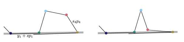
Figure 13. Paths with a tube incidence at $(1,5)$, so that $|y_{5}-(y_{1}+sp_{1})|\lessapprox r$ for some $s\in{\mathbf{R}}$. On the left, an example in which $p_{4}$ is transverse to $p_{1}$. In this case the time variable $s_{4}$ is constrained so that $y_{5}$ can lie on the gray tube. On the right, an example in which $p_{4}$ is approximately parallel to $p_{1}$. In this case $s_{4}$ is much less constrained, but $p_{4}$ is much more constrained. In either case there is a gain of a factor of (at least) ${\varepsilon}^{1/2}$.

Lemma 4.19 (The tube incidence bound).

Let $A$ be an admissible operator, let $k_{+},k_{-}\in[k_{max}]$, let $P,Q\in{\mathcal{P}}([k_{+}]\sqcup[k_{-}])$, and let $I^{tube}\not=\varnothing$ be a nonempty set of tube incidences in $[k_{+}]$, and suppose moreover that $I^{rec}=\varnothing$ so that there are no recollisions.

(4.27) $$\sup_{\xi_{0}^{-}}\Big{|}\int\mathinner{\langle{\xi_{1}^{-}|A|\xi_{1}^{+}}\rangle}\Xi(\Gamma)E_{Q\vee P}(\bm{\Gamma}){\mathbf{1}}_{P}(\bm{\Gamma}){\mathbf{1}}_{I^{rec}}(\bm{\Gamma})\mathop{}\!\mathrm{d}\omega^{\pm}\mathop{}\!\mathrm{d}\xi_{1}^{\pm}\mathop{}\!\mathrm{d}\xi_{0}^{-}\Big{|}\leq C^{k_{+}+k_{-}}({\varepsilon}^{2}\tau)^{(k_{+}+k_{-})/2}({\varepsilon}^{-1.5}\tau^{-1}).$$

Proof.

Let $(a,a^{\prime})\in I^{tube}$ be a tube incidence in $\omega^{+}$. Let $b<a^{\prime}$ be the last collision before $a^{\prime}$ that does not belong to an immediate recollision, so that $|y_{a^{\prime}}-(y_{b}+(t_{a^{\prime}}-t_{b})p_{b})|\leq C\alpha^{10}r$ We decompose the indicator function for the tube incidence according to the angle between $p_{b}$ and $p_{a}$,

$${\mathbf{1}}_{I^{tube}}(\bm{\Gamma})\leq {\mathbf{1}}(|(y_{a}+sp_{a})-(y_{b}+(t_{a^{\prime}}-t_{b})p_{b^{\prime}})|\leq 100k^{4}\alpha^{20}r\text{ for some }s\in{\mathbf{R}}){\mathbf{1}}(\theta(p_{a},p_{b})\geq\delta)$$

$$+{\mathbf{1}}(\theta(p_{a},p_{b})\leq\delta),$$

where $\theta(u,v):=\min\{|u/|u|-v/|v||,|u/|u|+v/|v||\}$, and $\delta$ is a small parameter that we will optimize shortly.

This splits the integral as a sum of two terms. In the first term, we use the fact that the set of times for which the bound

$$|(y_{a}+sp_{a})-(y_{b}+(t_{a^{\prime}}-t_{b})p_{b^{\prime}})|\leq 100k^{4}\alpha^{20}r$$

holds is an interval with width at most $C\alpha^{20}r(|p_{0}|\theta(p_{a},p_{b}))^{-1}$, and so we obtain this factor instead of $\tau$ in the integration over the $s_{a^{\prime}-1}$ variable.

In the second term, we gain a factor of $\delta^{d-1}$ as the integration over the annulus contributes $r^{-1}\delta^{d-1}|p_{0}|^{d-1}$ rather than $r^{-1}|p_{0}|^{d-1}$. Therefore

(4.28) $$\begin{split}\sup_{\xi_{0}^{-}}\Big{|}&\int\mathinner{\langle{\xi_{1}^{-}|A|\xi_{1}^{+}}\rangle}\Xi(\Gamma)E_{Q\vee P}(\bm{\Gamma}){\mathbf{1}}_{P}(\bm{\Gamma}){\mathbf{1}}(|y_{a}-y_{b}|\leq 2r){\mathbf{1}}(|y_{b-1}-y_{b}|\geq Kr)\mathop{}\!\mathrm{d}\omega^{\pm}\mathop{}\!\mathrm{d}\xi_{1}^{\pm}\mathop{}\!\mathrm{d}\xi_{0}^{-}\Big{|}\\ &\qquad\leq C^{k_{+}+k_{-}}{\varepsilon}^{k_{+}+k_{-}}\tau^{|P|}\min\{[C\alpha^{20}r\tau^{-1}(|p_{0}|\delta)^{-1}+\delta^{d-1})].\end{split}$$

Choosing $\delta={\varepsilon}^{1/d}$ produces an extra factor of ${\varepsilon}^{d-1/d}\leq{\varepsilon}^{1/2}$, as desired. ∎

5. Iterating the path integral

In this section we set up the path integral we use to reach diffusive times $N\tau={\varepsilon}^{-2-9\kappa/10}$. In this section we focus on the main term

$${\widetilde{{\mathcal{E}}}}_{N\tau}[A]={\mathbf{E}\,}(U_{\tau,\sigma}^{N})^{*}AU_{\tau,\sigma}^{N}.$$

Each of the operators $U_{\tau}$ is expanded as an integral over path segments. Together these path segments form an elongated path that we call an extended path. An extended path is a tuple of path segments interspered with phase space points $\xi_{\ell}$, as follows

$$\Gamma=(\xi_{0},\omega_{1},\xi_{1},\xi_{2},\omega_{2},\xi_{3},\cdots,\xi_{2\ell-2},\omega_{\ell},\xi_{2\ell-1},\cdots,\xi_{2N-2},\omega_{N},\xi_{2N-1}).$$

We sometimes also reorder $\Gamma$ as a tuple of phase space points $\bm{\xi}$ and path segments $\bm{\omega}$, so $\Gamma=(\bm{\xi},\bm{\omega})\in({{\mathbf{R}}^{2d}})^{2N}\times\Omega(\tau)^{N}$. We write $\Omega_{ext}^{N}$ to denote this space of extended paths.

The extended paths that will actually contribute to our integral satisfy additional compaibility conditions that ensure that the phase space endpoints of the segments match up nicely. We define the set $\Omega_{\alpha,S}^{N}\subset\Omega_{ext}^{N}$ to be

$$\Omega_{\alpha,S}^{N}:=\{\Gamma=(\bm{\xi},\bm{\omega})\in({{\mathbf{R}}^{2d}})^{2N}\times\Omega^{N}\mid\omega_{\ell}\in\Omega_{\alpha}(\tau,S;\xi_{2\ell-2},\xi_{2\ell-1})\text{ and }d_{r}(\xi_{2\ell-1},\xi_{2\ell})<N^{2}\}.$$

Note that the superscript $N$ in $\Omega_{\alpha,S}^{N}$ is just notation – the set is not itself a Cartesian product of $N$ copies of $\Omega_{\alpha,S}$.

We will be integrating over paths, which means we need to specify a measure. Give $\Omega_{k}$ the measure $d_{k}\omega$ which is the Lebesgue measure on $\triangle_{k+1}(\tau)\times({\mathbf{R}}^{d})^{k+1}\times({\mathbf{R}}^{d})^{k}$. Then we assign $\Omega$ the measure formed on the union, so that given a continuous function $f\in C^{0}(\Omega)$,

$$\int_{\Omega}f(\omega)\mathop{}\!\mathrm{d}\omega:=\sum_{k=0}^{k_{max}}\int_{\Omega_{k}}f(\omega)\mathop{}\!\mathrm{d}_{k}\omega.$$

The measure $\mathop{}\!\mathrm{d}\omega$ allows us to define the measure $\mathop{}\!\mathrm{d}\Gamma$, informally written

$$\mathop{}\!\mathrm{d}\Gamma=\prod_{\ell=0}^{2N-1}\mathop{}\!\mathrm{d}\xi_{\ell}\prod_{\ell=1}^{N}\mathop{}\!\mathrm{d}\omega_{\ell}.$$

Note that each path $\Gamma\in\Omega_{\alpha,S}^{N}$ specifies a collision number sequence ${\mathbf{k}}(\Gamma)=(k_{1},\cdots,k_{N})$, where $k_{\ell}$ is the number of collisions in the segment $\omega_{\ell}$. Thus integration over $\Omega_{\alpha,S}^{N}$ implicitly includes a sum over ${\mathbf{k}}$.

We define a smooth cutoff $\Xi$ on the space of extended paths that has support in $\Omega_{\alpha,S}$, defined by

$$\Xi(\Gamma)=\prod_{\ell=1}^{N}\chi_{\alpha,S}(\omega_{\ell},\xi_{2\ell-2},\xi_{2\ell-1}).$$

The collisions in a path $\Gamma\in\Omega_{ext}^{N}$ are indexed by pairs $(\ell,j)$ indicating the segment index $\ell$ and the collision index $j$ within the segment. So that we can index all of the collisions at once, we use the collision index set

$$K(\Gamma)=\{(\ell,j)\mid\ell\in[1,N]\text{ and }j\in[1,k_{j}]\}.$$

Sometimes we also need $K_{0}(\Gamma)$ which is

$$K_{0}(\Gamma)=\{(\ell,j)\mid\ell\in[1,N]\text{ and }j\in[0,k_{j}]\}.$$

We will use letters like $a,b,c$ to refer to the indices in $K(\Gamma)$. Also, we impose a ordering on $K$ using the lexicographic order, and write $a+_{K}1$ to mean the successor of the index $a$ in the collision set $K(\Gamma)$. The index set $K_{all}$ refers to the set of all possible collision indices

$$K_{all}=[1,N]\times[1,k_{max}]=\{(\ell,j)\mid\ell\in[1,N],j\in[1,k_{max}]\}.$$

We define the function $\ell:K_{all}\to[1,N]$ which sends $a=(\ell,j)$ to $\ell(a)=\ell$, which we also call the segment index of the collision index $a$.

The path $\Gamma$ defines an operator $O_{\Gamma}$

(5.1) $$O_{\Gamma}=\mathinner{|{\xi_{0}}\rangle}\mathinner{\langle{\xi_{2N-1}}|}\prod_{\ell=1}^{N}\mathinner{\langle{\xi_{2\ell-2}|O_{\omega_{\ell}}|\xi_{2\ell-1}}\rangle}\prod_{\ell=1}^{N-1}\mathinner{\langle{\xi_{2\ell-1}|\xi_{2\ell}}\rangle}.$$

To write down an expression of ${\mathcal{E}}_{N\tau}[A]$ we will integrate over pairs of paths $(\Gamma^{+},\Gamma^{-})$, and will therefore need to index into the path variables of both paths simultaneously. We therefore define the signed index sets $K^{+}(\Gamma)$ and $K^{-}(\Gamma)$, with

$$K^{\pm}(\Gamma)=\{(\ell,j,\pm)\mid(\ell,j)\in K(\Gamma)\}.$$

This allows us to define the doubled index set

$${\mathbf{K}}(\Gamma^{+},\Gamma^{-})=K^{+}(\Gamma^{+})\sqcup K^{-}(\Gamma^{-})$$

Analagously, we write ${\mathbf{K}}_{all}=K_{all}^{+}\sqcup K_{all}^{-}$. The set ${\mathbf{K}}_{all}$ has a partial ordering induced by the ordering on $K_{all}$, with $(a,+)$ being incomparable to $(a^{\prime},-)$ for any $a,a^{\prime}\in K_{all}$. Moreover, we write $\operatorname{sgn}(a)$ to be the “sign” of an index in ${\mathbf{K}}$ (so $\operatorname{sgn}(a)=+1$ if $a\in K^{+}_{all}$ and $\operatorname{sgn}(a)=-1$ if $a\in K^{-}_{all}$). Finally, given an index $a=(\ell,\pm,j)$, we write $a^{*}$ for the index of opposite sign, so $a^{*}=(\ell,\mp,j)$.

These signed collision indices will be used to index into doubled paths, $\bm{\Gamma}=(\Gamma^{+},\Gamma^{-})$. Now there is an abuse of notation we will sometimes use, which is that we will sometimes go back and forth between signed and unsigned indices when the path $\Gamma$ is fixed (either being $\Gamma^{+}$ or $\Gamma^{-}$).

We can now write down an integral expression for ${\widetilde{{\mathcal{E}}}}_{N\tau}[A]$,

$${\widetilde{{\mathcal{E}}}}_{N\tau}[A]=\int_{\Omega_{\alpha,S}^{N}\times\Omega_{\alpha,S}}\Xi(\Gamma^{+})\Xi(\Gamma^{-}){\mathbf{E}\,}O_{\Gamma^{-}}^{*}AO_{\Gamma^{+}}\mathop{}\!\mathrm{d}\bm{\Gamma},$$

with an error on the order $O({\varepsilon}^{0.1}\|A\|_{op})$ in operator norm. We further restrict to pairs of paths $(\Gamma^{+},\Gamma^{-})$ that produce a nonnegligible contribution to ${\mathbf{E}\,}O_{\Gamma^{-}}^{*}AO_{\Gamma^{+}}$. The naive bound on the operator norm coming from applying the triangle inequality and estimating volumes is on the order $O({\varepsilon}^{-CN})$, and therefore we will have to consider any pairs of paths $(\Gamma^{+},\Gamma^{-})$ satisfying

$$\|{\mathbf{E}\,}O_{\Gamma^{-}}^{*}AO_{\Gamma^{+}}\|_{op}\geq{\varepsilon}^{CN}.$$

Expanding the operator $O_{\Gamma}$ using the definition (5.1) and (3.1), and simply bounding all deterministic quantities with an appropriate factor of ${\varepsilon}^{-C}$, we obtain a simple bound

(5.2) $$\begin{split}\|{\mathbf{E}\,}O_{\Gamma^{-}}^{*}AO_{\Gamma^{+}}\|_{op}&\leq|\mathinner{\langle{\xi_{0}^{+}|A|\xi_{0}^{-}}\rangle}|{\mathbf{E}\,}\prod_{\ell=1}^{N}\mathinner{\langle{\xi_{2\ell-2}^{+}|O_{\omega_{\ell}^{+}}|\xi_{2\ell-1}^{+}}\rangle}^{*}\mathinner{\langle{\xi_{2\ell-2}^{-}|O_{\omega_{\ell}^{-}}|\xi_{2\ell-1}^{-}}\rangle}\\ &\leq{\varepsilon}^{-CN}|\mathinner{\langle{\xi_{0}^{+}|A|\xi_{0}^{-}}\rangle}|{\mathbf{E}\,}\prod_{a\in K(\Gamma^{+})}{\widehat{V_{y_{a}^{+}}}}(p_{a}^{+}-p_{a-1}^{+})^{*}\prod_{a\in K(\Gamma^{-})}{\widehat{V_{y_{a}^{-}}}}(p_{a}^{-}-p_{a-1}^{-}).\end{split}$$

First we rewrite the expression above using signed indices $a$, defining the impulse variables $q_{a}=p_{a}-p_{a-1}$ when $a\in K^{+}(\Gamma^{+})$ and $q_{a}=p_{a-1}-p_{a}$ for $a\in K^{-}(\Gamma^{-})$. Then, because the potential $V$ is real and therefore ${\widehat{V}}(q)^{*}={\widehat{V}}(-q)$, we can write more succinctly

$${\mathbf{E}\,}\prod_{a\in K(\Gamma^{+})}{\widehat{V_{y_{a}^{+}}}}(p_{a}^{+}-p_{a-1}^{+})^{*}\prod_{a\in K(\Gamma^{-})}{\widehat{V_{y_{a}^{-}}}}(p_{a}^{-}-p_{a-1}^{-}).={\mathbf{E}\,}\prod_{a\in K(\bm{\Gamma})}{\widehat{V_{y_{a}}}}(q_{a}).$$

We can split the expectation using the geometry of the points $y_{a}$. More precisely, given $\bm{\Gamma}$ we define a graph $G(\bm{\Gamma})$ on the vertex $K(\bm{\Gamma})$ in which $(a,b)$ is an edge of $G(\bm{\Gamma})$ when $|y_{a}-y_{b}|\leq 2r$. The graph $G(\bm{\Gamma})$ then defines a partition $P(\bm{\Gamma})\in{\mathcal{P}}(K(\bm{\Gamma}))$ which is the partition of collisions into the connected components of the graph. Since $V_{y_{a}}$ is independent of $V_{y_{b}}$ when $|y_{a}-y_{b}|\geq 2r$, we can split the expectation using the partition $P(\bm{\Gamma})$,

(5.3) $${\mathbf{E}\,}\prod_{a\in K(\bm{\Gamma})}{\widehat{V_{y_{a}}}}(q_{a}).=\prod_{S\in P(\bm{\Gamma})}{\mathbf{E}\,}\prod_{a\in S}{\widehat{V_{y_{a}}}}(q_{a}).$$

The moment bound on the Fourier coefficients ${\widehat{V_{y_{a}}}}$ in particular implies that for any sequence $(y_{j},q_{j})\in{{\mathbf{R}}^{2d}}$,

$$\big{|}{\mathbf{E}\,}\prod_{j=1}^{k}{\widehat{V_{y_{j}}}}(q_{j})\big{|}\leq{\varepsilon}^{-Ck}k^{Ck}\exp(-c(k^{-1}r|\sum_{j}q_{j}|)^{0.99}).$$

This crude estimate places already a significant constraint on the geometry of the paths $\bm{\Gamma}$ that contribute to the evolution operator ${\mathcal{E}}_{N\tau}$. We say that a pair of paths $\bm{\Gamma})$ is $\beta$-complete if for every $S\in P(\bm{\Gamma})$, $|\sum_{j\in S}q_{j}|\leq\beta r$.

The calculation above shows the following

Lemma 5.1.

For a band-limited operator $A$ and $\beta=N^{4}$,

$$\|\int_{\Omega_{\alpha,S}^{N}\times\Omega_{\alpha,S}^{N}}\Xi(\Gamma^{+})\Xi(\Gamma^{-})(1-{\mathbf{1}}_{\bm{\Gamma}\textrm{ is }\beta-\text{complete}}){\mathbf{E}\,}O_{\Gamma^{-}}^{*}AO_{\Gamma^{+}}\mathop{}\!\mathrm{d}\bm{\Gamma}\|_{op}\leq{\varepsilon}^{100}\|A\|_{op}.$$

Proof.

The bound follows from an application of the Schur test in the wavepacket basis, along with the estimate

$$|\langle{\xi_{2N-1}^{+}|{\mathbf{E}\,}O_{\Gamma^{-}}^{*}AO_{\Gamma^{+}}|\xi_{2N-1}^{-}}\rangle|\leq{\varepsilon}^{-CN}|\langle{\xi_{0}^{+}|A|\xi_{0}^{-}}\rangle|\exp(-cN^{2})$$

for paths $(\Gamma^{+},\Gamma^{-})$ which are not $N^{4}$-complete. ∎

For convenience we simply write $\Gamma^{+}\sim\Gamma^{-}$ when $\bm{\Gamma}$ is $N^{4}$-complete.

In the next section we explore in more detail the geometric features of paths $\bm{\Gamma}$ which are $N^{4}$-complete.

6. Geometry and combinatorics of extended paths

The point of this section is to more precisely specify the relationship between the geometry of paths (as described by their “events”) and the combinatorial properties of the collision partition that the paths induce. Our end goal is to derive a diagrammatic expansion for ${\mathcal{E}}_{N\tau}$ which is stratified by a measure of combinatorial complexity that matches geometric complexity. The geometric complexity will allow us to bound complicated diagrams by additional factors of ${\varepsilon}^{c}$, which is needed to reach diffusive times.

6.1. From extended paths to concatenated paths

For the arguments in this section it will be easier to work with a single “concatenated path” rather than an extended path. We will therefore define a map

$$\bm{\omega}=(\omega_{1},\omega_{2},\cdots,\omega_{N})\mapsto({\mathbf{S}},{\mathbf{P}},{\mathbf{Y}})$$

that sends sequences of path segments to a single path. Given such a sequence $\bm{\omega}$, let $K_{0}(\bm{\omega})$ be the collision indexing set

$$K_{0}(\bm{\omega})=\{(\ell,j)\mid\ell\in[1,N],j\in[0,k_{\ell}]\}$$

and $K(\bm{\omega})=K_{0}(\bm{\omega})\setminus([1,N]\times\{0\})$. Then, given $\bm{\omega}$ we define ${\mathbf{S}}$ by

$$S_{j}:=\sum_{\begin{subarray}{c}b\in K_{0}(\bm{\omega})\\ a_{j}\leq b<a_{j+1}\end{subarray}}s_{b},$$

where $a_{j}$ is the $j$-th element of $K(\bm{\omega})$, with the convention that $a_{0}=0$ and $a_{(\sum k_{j})+1}=\infty$ are minimal and maximal elements, respectively. An alternative definition of $S_{j}$ starts by defining the collision times $T_{\ell,j}$ for each collision in $\omega_{\ell}$, by

$$T_{\ell,j}=\ell\tau+\sum_{j^{\prime}<j}s_{\ell,j^{\prime}}.$$

Then $S_{a}$ satisfies $S_{a}=T_{a+1}-T_{a}$ (with the convention that $T_{1,0}=0$ and $T_{N,k_{N}}=N\tau$). We can also assign the momentum variables for each $a\in K_{{\mathbf{k}}}$ by setting $P_{a}=p_{a}$, and also $P_{1,0}=p_{1,0}$. Finally, $Y_{a}=y_{a}$.

The following lemma shows that the concatenated path $({\mathbf{S}},{\mathbf{P}},{\mathbf{Y}})$ approximately satisfies the compatibility conditions and approximate conservation of energy expected of a single path segment.

Lemma 6.1 (Path concatenation lemma).

If $\Gamma=(\bm{\xi},\bm{\omega})\in\Omega_{\alpha,S}^{N}$ is an extended path then the concatenated path $({\mathbf{S}},{\mathbf{P}},{\mathbf{Y}})$ formed from the tuple $\bm{\omega}$ satisfies the compatibility condition

(6.1) $$|Y_{a+1}-(Y_{a}+S_{a}P_{a})|\leq C\alpha(r+S_{a}^{2}\tau^{-1}r^{-1}+S_{a}\tau^{-1}r).$$

for each $a\in K(\Gamma)$, as well as the conservation of kinetic energy conditions

(6.2) $$||P_{a}|^{2}/2-|P_{a^{\prime}}|^{2}/2||\leq\alpha\max\{S_{a}^{-1},S_{a^{\prime}}^{-1},|P_{a}|r^{-1}\}+\alpha|T_{a}-T_{a^{\prime}}|\tau^{-1}r^{-1}.$$

for $a,a^{\prime}\in K(\Gamma)$.

Combining Lemma 6.1 with the argument of Lemma 4.5, we obtain the following corollary

Corollary 6.2.

Let $\bm{\Gamma}=(\Gamma^{+},\Gamma^{-})\in\Omega_{\alpha,S}^{N}\times\Omega_{\alpha,S}^{N}$ be a pair of paths that is $N^{4}$ complete, and let $({\mathbf{S}}^{+},{\mathbf{P}}^{+},{\mathbf{Y}}^{+})$ be the concatenated path formed from $\Gamma^{+}$. Suppose that $a,a^{\prime}\in K(\Gamma^{+})$ are two collision indices such that for all $a<b<a^{\prime}$, either $\{b,b-1\}\in P(\bm{\Gamma})$ or $\{b,b+1\}\in P(\bm{\Gamma})$. Then

$$|Y_{a^{\prime}}-(Y_{a}+(T_{a^{\prime}}-T_{a})P_{a})|\leq 100k_{max}^{2}N^{6}r.$$

To prove Lemma 6.1 we first need an elementary result showing that the kinetic energy cannot drift too much between the endpoints of a path segment.

Lemma 6.3.

If $\omega=({\mathbf{s}},{\mathbf{p}},{\mathbf{y}})\in\Omega_{\alpha,k}(\tau,\sigma;\eta,\xi)$ and $|\xi_{p}|\geq r\sigma^{-1}$, then $||\xi_{p}|^{2}/2-|\eta_{p}|^{2}/2|\leq\alpha|\xi_{p}|r^{-1}$. In particular, $||\xi_{p}|-|\eta_{p}||\leq\alpha r^{-1}$.

Proof.

For $\omega$ to be $\alpha$-compatible with $\eta$ and $\xi$ it follows that $|p_{0}-\xi_{p}|\leq\alpha r^{-1}$ and $|p_{k}-\eta_{p}|\leq\alpha r^{-1}$. Moreover, since $s_{0},s_{k}\geq S$, it follows from the kinetic energy condition that

$$||p_{0}|^{2}/2-|p_{k}|^{2}/2|\leq\alpha\min\{\sigma^{-1},|\xi_{p}|r^{-1}\}\leq\alpha|\xi_{p}|r^{-1}.$$

The conclusion that $||\xi_{p}|-|\eta_{p}||\leq\alpha r^{-1}$ follows from an elementary argument. ∎

Proof.

For each $\ell\in[1,N]$, set

$$z_{\ell}:=\begin{cases}(\xi_{\ell})_{x}-(y_{\ell,k_{\ell}}+s_{\ell,k_{\ell}}p_{\ell,k_{\ell}}),&k_{\ell}>0\\ (\xi_{\ell})_{x}-(\xi_{\ell-1})_{x}+\tau p_{\ell,0},&k_{\ell}=0.\end{cases}$$

Moreover, for $a\in K(\Gamma)$, set

$$z_{a}=\begin{cases}y_{a}-(y_{a-1}+s_{a-1}p_{a-1}),&a=(\ell,j)\text{ for some }j>1,\ell\in[1,N]\\ y_{\ell,1}-((\xi_{\ell})_{x}+s_{\ell,0}p_{\ell,0}),&a=(\ell,0)\text{ for some }\ell\in[1,N].\end{cases}$$

The idea is that these ‘$z$’ variables represent the offset in the collision positions and the “checkpoints” $\xi_{\ell}$. We also need to keep track of the offset in the momenta variables, so similarly we define

$$u_{\ell}^{-}:=(\xi_{\ell})_{p}-p_{\ell,k_{\ell}}$$

and

$$u_{\ell}^{+}:=p_{\ell+1,0}-(\xi_{\ell})_{p}.$$

Because $\Gamma\in\Omega_{\alpha,{\mathbf{k}}}(\tau,S)$, each of the $z$ variables satisfies $|z_{b}|\leq\alpha r$, and each of the $u$ variables satisfies $|u_{\ell}^{\pm}|\leq\alpha r^{-1}$. We can use these error variables to write

$$Y_{j+1}=Y_{j}+S_{j}P_{j}+\sum u_{\ell}^{+}s_{\ell}^{+}+\sum u_{\ell}^{-}s_{\ell}^{-}+\sum z_{b},$$

where the sum over $u_{\ell}^{\pm}$ includes all $\ell$ in between the collisions $a_{j}$ and $a_{j+1}$ (of which there are at most $k_{max}S_{j}\tau^{-1}$) and the times $s_{\ell}^{+}$ are all bounded by $S_{j}$. Moreover the sum over position displacements $z_{b}$ includes at most $S_{j}\tau^{-1}$ elements (one for each displacement at a checkpoint, and a final one for the collision $z_{a_{j}}$ itself. The bound then follows immediately.

The bound on the conservation of kinetic energy follows from applying Lemma 6.3 on each segment between the segments containing the collisions $a$ and $a^{\prime}$, of which there are $|T_{a}-T_{a^{\prime}}|\tau^{-1}$. ∎

6.2. Geometric features of paths

We have already seen in (5.3) that the partition $P(\bm{\Gamma})$, which is determined by the geometric configuration of the positions $y_{a}$ for $a\in K(\Gamma)$, determines how the expectation ${\mathbf{E}\,}O_{\Gamma}^{*}AO_{\Gamma}$ splits. The fundamental idea of this paper is that the extra compatibility conditions and conservation of kinetic energy conditions that an extended path satisfy significantly constrain the geometry of paths $\bm{\Gamma}$ that are $N^{4}$-complete.

The big idea of this paper is that the partition $P(\bm{\Gamma})$ can be significantly constrained using much less information than the full dependency graph $G(\bm{\Gamma})$ of the scattering locations. Specifically, we need only record pairs of collisions involved in certain rare events. The first kind of event is a recollision.

Definition 6.4 (Recollisions of extended paths).

The recollision graph $R(\bm{\Gamma})$ of an extended path $\bm{\Gamma}$ consists of all pairs $(a,a^{\prime})\subset K(\bm{\Gamma})$ such that $\operatorname{sgn}(a)=\operatorname{sgn}(a^{\prime})$, $a^{\prime}\not=a\pm 1$, and $|y_{a}-y_{a^{\prime}}|\leq 2r$.

We also define the set $E^{imm}(\bm{\Gamma})$ of immediate recollisions to be pairs $(a,a^{\prime})$ with $a^{\prime}=a\pm 1$ and $|y_{a}-y_{a^{\prime}}\leq 2r$.

The second kind of event is what we call a ladder-breaking event. A ladder-breaking event is a pair $(a,a^{\prime})$ of non-consecutive collisions for which it is possible to enter $a$ at some momentum $v$ and travel to the collision $a^{\prime}$. This can be encoded as a geometric constraint on the collision data $(y_{a},q_{a})$ and $(y_{a^{\prime}},q_{a^{\prime}})$.

Definition 6.5 (Ladder-breaking events).

The ladder-breaking event set $\operatorname{LB}(\bm{\Gamma})$ is the set of all pairs $(a,a^{\prime})\in K(\bm{\Gamma})^{2}$ such that there exists $b\in K(\bm{\Gamma})$ with $a<b<a^{\prime}$ and $b$ not belonging to an immediate recollision, and such that there exists $v\in{\mathbf{R}}^{d}$ and $t\in{\mathbf{R}}$ such that

$$||v|^{2}/2-|p_{1,0}|^{2}/2| \leq\alpha^{2}N^{10}|p_{1,0}|r^{-1}$$

$$||v-q_{a}|^{2}/2-|p_{1,0}|^{2}/2| \leq\alpha^{2}N^{10}|p_{1,0}|r^{-1}$$

$$||v+q_{a^{\prime}}|^{2}/2-|p_{1,0}|^{2}/2| \leq\alpha^{2}N^{10}|p_{1,0}|r^{-1}$$

$$|y_{a}+tv-y_{a^{\prime}}| \leq\alpha^{2}N^{10}r.$$

In addition, we say that $(0,a)$ forms a ladder-breaking event if there exists $b\in K(\bm{\Gamma})\setminus I^{imm}(\bm{\Gamma})$ such that $b<a$ and there exists $t\in{\mathbf{R}}$ such that

$$||p_{1,0}+q_{a}|^{2}/2-|p_{1,0}|^{2}/2| \leq\alpha^{2}N^{10}|p_{1,0}|r^{-1}$$

$$|y_{0}+tp_{1,0}-y_{a}| \leq\alpha^{2}N^{10}r.$$

Ladder breaking events themselves are difficult to work with because they cannot be determined solely by the collision data $(y_{a},q_{a})$ and $(y_{b},q_{b})$, but instead have an additional nonlocal constraint that every collision $a<a^{\prime}<b$ is an immediate recollision. We can simplify this by working with two other sets of local events that together cover the set of ladder-breaking events.

The first of these is a tube event, which is similar to the tube event we have already seen.

Definition 6.6 (Tube events).

A tube event in a path $\Gamma$ is a pair $(a,b)$ with $a<b$ and $a,b\not\in E^{imm}(\Gamma)$ satisfying the condition that there exists $s\in{\mathbf{R}}$ such that

$$|y_{b}-(y_{a}+sp_{a-1})|\leq N^{12}r.$$

We write $E^{tube}(\Gamma)$ for the set of all tube events.

The other type of event is called a cone event. Cone events are more complicated, and an example is visualized in Figure 14.

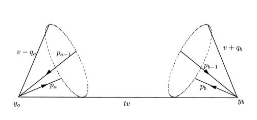
Figure 14. A depiction of a cone event at $(a,b)$. The collision site $y_{b}$ does not lie near the ray $y_{a}+sp_{a}$ (which points out of the page), but there does exist some momentum $v$ for which $y_{b}\approx y_{a}+tv$, and so that both $v-q_{a}$ and $v+q_{a}$ have approximately the correct kinetic energy. This occurs when the cone drawn at $y_{a}$ which contains the rays $y_{a}+sp_{a}$ and $y_{a}+sp_{a-1}$ also contains the point $y_{b}$ and vice-versa, hence the name.

Definition 6.7 (Cone events).

A cone event in a path $\Gamma$ is a pair $(a,b)$ with $a<b$ such that there exists $v\in{\mathbf{R}}^{d}$ and $s\in{\mathbf{R}}$ such that

$$||v|^{2}/2-|p_{1,0}|^{2}/2| \leq\alpha^{2}N^{10}|p_{1,0}|r^{-1}$$

$$||v-q_{a}|^{2}/2-|p_{1,0}|^{2}/2| \leq\alpha^{2}N^{10}|p_{1,0}|r^{-1}$$

$$||v+q_{a^{\prime}}|^{2}/2-|p_{1,0}|^{2}/2| \leq\alpha^{2}N^{10}|p_{1,0}|r^{-1}$$

$$|y_{a}+tv-y_{a^{\prime}}| \leq\alpha^{2}N^{10}r,$$

and moreoever $|v-p_{a}|\geq N^{8}r^{-1}$. We write $E^{cone}(\Gamma)$ for the set of all cone events.

We observe that the tube events and cone events “cover” the ladder-breaking events.

Lemma 6.8.

Let $(a,b)\in\operatorname{LB}(\bm{\Gamma})$. Then either $(a,b)\in E^{cone}(\Gamma)$ or there exists $c$ such that $a<c<b$ and $(c,b)\in E^{tube}(\Gamma)$.

Proof.

Suppose that $(a,b)\in\operatorname{LB}(\bm{\Gamma})\setminus E^{cone}(\Gamma)$. Then in particular $p_{a}$ itself satisfies $|y_{a}+sp_{a}-y_{b}|\leq N^{10}r$. Let $a^{\prime}$ be the collision index satisfying $a<a^{\prime}<b$ and such that $a^{\prime}$ is not an immediate recollision. Then $(a^{\prime},b)$ is a tube event. ∎

The final piece of information we need is a trimmed form of the recollision graph $G(\bm{\Gamma})$ that removes all isolated edges. Recall that the dependency graph $G(\bm{\Gamma})$ is defined to be

$$G(\bm{\Gamma})=\{(a,b)\in\binom{K(\bm{\Gamma})}{2}\mid|y_{a}-y_{b}|\leq 2r\}.$$

We use the graph $G(\bm{\Gamma})$ to define the cluster graph $C(\bm{\Gamma})$ below.

Definition 6.9 (Cluster graph).

The cluster graph $C(\bm{\Gamma})$ of a doubled path $\bm{\Gamma}$ is defined to be

$$G_{C}(\bm{\Gamma}):=\{(a,b)\in G(\bm{\Gamma})\mid\text{ there exists }c\in K(\bm{\Gamma})\setminus\{a,b\}\text{ such that }(a,c)\in G(\bm{\Gamma})\text{ or }(b,c)\in G(\bm{\Gamma})\}.$$

We write $\operatorname{supp}G_{C}(\bm{\Gamma})$ to mean the set of indices contained in an edge of $C(\bm{\Gamma})$.

We say that a collision index $a\in K(\bm{\Gamma})$ is typical if there does not exist $b\sim_{P(\bm{\Gamma})}a$ such that $b$ belongs to a recollision, tube, or cone event, or a cluster in $C(\bm{\Gamma})$. We write $\operatorname{Typ}(\bm{\Gamma})$ for the set of typical indices.

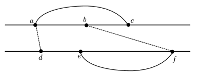
Figure 15. An abstract representation of the geometric data of a path. In this depiction, $(a,c)$ forms a recollision as well as $(e,f)$, and $a\sim d$, $b\sim f$. Note that $b$ and $d$ are atypical collisions even though they do not belong to recollisions, tube events, or cone events.

6.3. Combinatorial consequences of events

In this section we see that the partition $P(\bm{\Gamma})$ has a rigid structure on the typical collision indices.

The main lemma is the following simple on the geometry of consecutive collisions. Given a path $\bm{\Gamma}$ and a collision index $a\in K(\bm{\Gamma})$, we define $\triangleright(a)\in K(\bm{\Gamma})$ to be the next collision index after $a$ that is not an immediate recollision, so

$$\triangleright(a):=\min\{a^{\prime}\in K(\bm{\Gamma})\mid a^{\prime}>a\text{ and }a^{\prime}\not\in E^{imm}(\bm{\Gamma})\}.$$

Likewise we set $\triangleleft(a)$ to be the collision prior to $a$ that is not an immediate recollision,

$$\triangleleft(a):=\min\{a^{\prime}\in K(\bm{\Gamma})\mid a^{\prime}<a\text{ and }a^{\prime}\not\in E^{imm}(\bm{\Gamma})\}.$$

Lemma 6.10.

Let $\bm{\Gamma}$ be an $N^{4}$-complete extended path, and let $a\in K(\Gamma^{+})$, $b,b^{\prime}\in K(\Gamma^{-})$ satisfy $\{a,b\},\{\triangleright(a),b^{\prime}\}\in P(\bm{\Gamma})$. Then the following inequalities hold:

$$||p_{a}|^{2}/2-|p_{1,0}|^{2}/2| \leq C\alpha^{2}N^{8}|p_{1,0}|r^{-1}$$

$$||p_{a}-q_{b}|^{2}/2-|p_{1,0}|^{2}/2| \leq C\alpha^{2}N^{8}|p_{1,0}|r^{-1}$$

$$||p_{a}+q_{b^{\prime}}|^{2}/2-|p_{1,0}|^{2}/2| \leq C\alpha^{2}N^{8}|p_{1,0}|r^{-1}$$

$$|y_{b}+(T_{\triangleright(a)}-T_{a})p_{a}-y_{b^{\prime}}| \leq C\alpha^{2}N^{8}r.$$

Proof.

The last inequality follows from Corollary 6.2 along with the bounds $|y_{a}-y_{b}|\leq 2r$ and $|y_{\triangleright(a)}-y_{b^{\prime}}|\leq 2r$ that follow from $\{a,b\},\{\triangleright(a),b^{\prime}\}\in P(\bm{\Gamma})$.

The first inequality follow from the kinetic energy conservation condition.

The second and third inequalities follow from the same kinetic energy conservation condition coupled with the bounds

$$|p_{\triangleright(a)}-(p_{a}+q_{b^{\prime}})| \leq N^{4}r^{-1}$$

$$|p_{a-1}-(p_{a}-q_{b})| \leq N^{4}r^{-1}$$

which follow from the condition that $\bm{\Gamma}$ is $N^{4}$-complete. ∎

We use Lemma 6.10 to obtain a local rigidity statement for the partition $P(\bm{\Gamma})$.

Lemma 6.11 (Ladder-forming lemma).

Let $\bm{\Gamma}$ be an $N^{4}$-complete extended path, and let $a\in K(\Gamma^{+})$, $b\in K(\Gamma^{-})$ be collisions satisfying $\{a,b\}\in P(\bm{\Gamma})$. Suppose further that $\{a,\triangleright(a)\}\subset\operatorname{Typ}(\bm{\Gamma})$ and $b$ does not belong to a ladder-breaking event of $\bm{\Gamma}$. Then either $\triangleright(a)\sim_{P(\bm{\Gamma})}\triangleright(b)$ or $\triangleright(a)\sim_{P(\bm{\Gamma})}\triangleleft(b)$.

Moreover, if $\{\triangleleft(a),a\}\subset\operatorname{Typ}(\bm{\Gamma})$, then either $\triangleleft(a)\sim_{P(\bm{\Gamma})}\triangleright(b)$ or $\triangleleft(a)\sim_{P(\bm{\Gamma})}\triangleleft(b)$.

Proof.

We will treat only the case $\{a,\triangleright(a)\}\subset\operatorname{Typ}(\bm{\Gamma})$, as the case $\{a,\triangleleft(a)\}\subset\operatorname{Typ}(\bm{\Gamma})$ is similar.

First, we observe that it must be the case that $\triangleright(a)\sim_{P(\bm{\Gamma})}b^{\prime}$ for some index $b^{\prime}\in K(\Gamma^{-})$, or else $\triangleright(a)$ would belong to a recollision and therefore not be typical. If $\{\triangleright(a),b^{\prime}\}\not\in P(\bm{\Gamma})$, then there is an additional collision belonging to the cluster containing $\{\triangleright(a),b\}$, so $\triangleright(a)\in\operatorname{supp}C(\bm{\Gamma})$ and therefore $\triangleright(a)\not\in\operatorname{Typ}(\bm{\Gamma})$.

We have therefore reduced to the case that $\{\triangleright(a),b^{\prime}\}\in P(\bm{\Gamma})$ for some $b^{\prime}\in K(\Gamma^{-})$. Now if $b^{\prime}$ is not $\triangleright(b)$ or $\triangleleft(b)$ then by Lemma 6.10 the pair $(b,b^{\prime})$ forms a ladder-breaking event, which is a contradiction. ∎

The final ingredient we need is a sufficient condition for the first collision of ${\widetilde{K}}^{+}$ to pair with the first collision of ${\widetilde{K}}^{-}$.

Lemma 6.12.

Suppose that $\bm{\Gamma}$ is an $N^{4}$-complete path with no ladder-breaking event of the form $(0,a)$, and suppose that $|p_{1,0,+}-p_{1,0,-}|\leq N\alpha$. Let $\triangleright^{+}(0)$ and $\triangleright^{-}(0)$ be the first collisions in $\Gamma^{+}$ and $\Gamma^{-}$, respectively, that are not immediate recollisions. If $\{\triangleright^{+}(0),\triangleright^{-}(0)\}\subset\operatorname{Typ}(\bm{\Gamma})$, then in fact $\{\triangleright^{+}(0),\triangleright^{-}(0)\}\in P(\bm{\Gamma})$.

Proof.

Since $\triangleright^{+}(0)\in\operatorname{Typ}(\bm{\Gamma})$, in particular it follows that $\{\triangleright^{+}(0),b\}\in P(\bm{\Gamma})$ for some $b\in K(\Gamma^{-})$. If $b\not=\triangleright^{-}(0)$, then one of $(0,b)$ or $(0,\triangleright^{-}(0))$ forms a ladder-breaking event. ∎

6.4. Global structure of the partition $P(\bm{\Gamma})$

Lemmas 6.11 and 6.12 provide only local information about the partition $P(\bm{\Gamma})$. We will turn this local information into a global rigidity result. The rigidity result we will prove is that the pairs formed by typical collisions can be partitioned into a small number of special partitions called ladder and anti-ladder matchings.

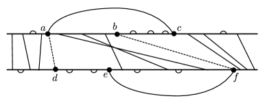
Figure 16. An example of a partition compatible with the geometric data of Figure 15. In this case the interval set is $\{(0,a),(a,b),(b,c),(c,\infty),(0,d),(d,e),(e,f),(f,\infty)\}$. The pair of intervals $\{(a,b),(e,f)\}$ forms a renormalized anti-ladder, and $(b,c)$ shows an example of a simple partition.

First we define ladders and anti-ladders in some generality.

Definition 6.13 (Ladders and anti-ladders).

Let $A$ and $B$ be two finite disjoint ordered sets with $|A|=|B|$. The ladder matching $P_{lad}\in{\mathcal{P}}(A\sqcup B)$ is the unique matching of the form $P_{lad}=\{\{a,\varphi(a)\}\}_{a\in A}$ where $\varphi:A\to B$ is the unique order-preserving bijection between $A$ and $B$. The anti-ladder matching is given by $\{\{a,\varphi^{-}(a)\}\}_{a\in A}$ with $\varphi^{-}$ being the unique order-reversing bijection.

Note that a partition $P\in{\mathcal{P}}(A\sqcup B)$ can be both a ladder and an anti-ladder if $|A|=|B|=1$.

The partition $P(\bm{\Gamma})$ can also have many instances of immediate recollisions, so we introduce renormalized ladders and anti-ladders to allow for immediate recollisions to exist between the “rungs” of the ladder.

Definition 6.14 (Renormalized ladders and anti-ladders).

Let $A$ and $B$ be two finite disjoint ordered sets. A renormalized ladder is any partition $P\in{\mathcal{P}}(A\sqcup B)$ for which there exist sets $I_{A}\subset A$ and $I_{B}\subset B$ satisfying the following properties:

• Every set $S\in P$ has exactly two elements, $|S|=2$. That is, $P$ is a matching.

• If $a,a^{\prime}\in A$ and $a\sim_{P}a^{\prime}$, then $a=a^{\prime}+_{A}1$ or $a^{\prime}=a+_{A}1$ and $a,a^{\prime}\in I_{A}$.

• Likewise, if $b,b^{\prime}\in B$ and $b\sim_{P}b^{\prime}$, then $b=b^{\prime}+_{B}1$ or $b^{\prime}=b+_{B}1$ and $b,b^{\prime}\in I_{B}$.

• The partition $P$ restricted to the set $(A\setminus I_{A})\sqcup(B\setminus I_{B})$ is a ladder partition.

Let ${\mathcal{Q}}_{rl}\subset{\mathcal{P}}(A\sqcup B)$ be the set of renormalized ladder partitions. We define renormalized anti-ladders in a similar way (that is, satisfying the first three conditions but so that $P$ restricted to $(A\setminus I_{A})\sqcup(B\setminus I_{B})$ is an anti-ladder). Let ${\mathcal{Q}}^{-}_{rl}$ denote the set of renormlized anti-ladder partitions.

The other important type of partition is a simple partition, which can be thought of as a ladder with no rungs.

Definition 6.15 (Simple partitions).

Let $A$ be a finite ordered set. The simple partition on $A$ is the perfect matching $M$ such that every pair $\{a,a^{\prime}\}\in M$ satisfies $a^{\prime}=a+_{A}1$ or $a=a^{\prime}+_{A}1$.

We will partition the index set $K(\bm{\Gamma})$ into a collection of intervals that cover the typical collision indices and an exception set of atypical collisions. Given an extended path $\bm{\Gamma}$ on a collision index set $K(\bm{\Gamma})$, and $a,b\in K(\bm{\Gamma})$ with $\operatorname{sgn}(a)=\operatorname{sgn}(b)$, we define the collision interval $(a,b)_{K(\bm{\Gamma})}$ to be the set of collisions

$$(a,b)_{K(\bm{\Gamma})}:=\{c\in K(\bm{\Gamma})\mid a<c<b\}.$$

We also define the “one-sided” intervals

$$(0,a)_{K(\bm{\Gamma})}:=\{c\in K(\bm{\Gamma})\mid c<a\}.$$

and

$$(a,\infty)_{K(\bm{\Gamma})}:=\{c\in K(\bm{\Gamma})\mid a<c\}.$$

In a similar way we can define closed intervals such as $[a,b]_{K(\bm{\Gamma})}$, which include the endpoints $a$ and $b$. We note that intervals are totally ordered sets, with an ordering inherited from the partial order on $K(\bm{\Gamma})$. We write $\operatorname{sgn}(I)$ to mean the sign of $I$, so that $\operatorname{sgn}((a,b)_{K(\bm{\Gamma})})=\operatorname{sgn}(a)=\operatorname{sgn}(b)$. An interval $(a,b)_{K(\bm{\Gamma})}$ is said to be typical with respect to $\bm{\Gamma}$ if $(a,b)_{K(\bm{\Gamma})}\subset\operatorname{Typ}(\bm{\Gamma})$. A maximal typical interval is a typical interval not strictly contained in any other typical interval. The maximal typical intervals are those of the form $(a,b)_{K(\bm{\Gamma})}$ for $a,b\not\in\operatorname{Typ}(\bm{\Gamma})$ or $(0,a)_{K(\bm{\Gamma})}$ or $(a,\infty)_{K(\bm{\Gamma})}$ for $a\not\in\operatorname{Typ}(\bm{\Gamma})$. We define ${\mathcal{I}}(\bm{\Gamma})$ to be the collection of maximal typical intervals defined on $\bm{\Gamma}$.

The main global result is that maximal typical intervals either form ladders, anti-ladders, or simple partitions.

Lemma 6.16.

Let $\bm{\Gamma}$ be an $N^{4}$-complete extended path, and let ${\mathcal{I}}(\bm{\Gamma})$ be its collection of maximal typical intervals. Then for each interval $I=(a,b)_{K(\bm{\Gamma})}\in{\mathcal{I}}$, at least one of the following holds:

• The interval $I$ forms a simple partition, in the sense that $P(\bm{\Gamma})$ is $I$-local and the restriction $P(\bm{\Gamma})|_{I}$ is a simple partition.

• There exists $I^{\prime}\in{\mathcal{I}}(\bm{\Gamma})$ with $\operatorname{sgn}(I)=-\operatorname{sgn}(I^{\prime})$ such that $P(\bm{\Gamma})$ is local to $I\cup I^{\prime}$ and $P|_{I\cup I^{\prime}}$ is either a renormalized ladder partition or a renormalized anti-ladder partition.

Proof.

Suppose that there exists $a\in I$ such that $a\sim_{P(\bm{\Gamma})}b$ for some $b\in K(\bm{\Gamma})$ with $\operatorname{sgn}(b)=-\operatorname{sgn}(a)$. Note that for such an index, $a\in{\widetilde{K}}(\bm{\Gamma})$. The collision index $b$ belongs to a unique interval $I^{\prime}$ with $\operatorname{sgn}(I^{\prime})=-\operatorname{sgn}(I)$. Then the fact that $P(\bm{\Gamma})|_{I\cup I^{\prime}}$ forms a ladder or an anti-ladder follows from repeated application of Lemma 6.11.

On the other hand, if $I$ does not contain any external collisions then we are in the first case, and $I$ must form a simple partition. ∎

6.5. Geometric features of ladders

We conclude this section by recording geometric features of paths that correlate along a ladder.

Lemma 6.17.

Let $\bm{\Gamma}$ be a $N^{4}$-complete path and suppose that $a\in K(\Gamma^{+})$, $b\in K(\Gamma^{-})$ are collision indices satisfying $\{a,b\}\in P(\bm{\Gamma})$ and $\{\triangleright(a),\triangleright(b)\}\in P(\bm{\Gamma})$. Then the following hold:

(6.3) $$|(t_{\triangleright(a)}-t_{a})-(t_{\triangleright(b)}-t_{b})| \leq CN^{6}|p_{1,0}|^{-1}r,$$

(6.4) $$|(p_{\triangleright(b)}-p_{\triangleright(a)})-(p_{b}-p_{a})| \leq CN^{4}r^{-1},$$

(6.5) $$|p_{a}-p_{b}| \leq N^{6}r(t_{\triangleright(a)}-t_{a})^{-1}.$$

Proof.

First observe that (6.4) is a direct consequence of the fact that $\bm{\Gamma}$ is $N^{4}$-complete.

The bounds (6.3) and (6.5) are less trivial. Now we prove (6.3). By Corollary 6.2,

$$|(y_{\triangleright(a)}-y_{a})-(t_{\triangleright(a)}-t_{a})p_{a}|\leq\alpha N^{6}r.$$

On the other hand, $|y_{\triangleright(a)}-y_{\triangleright(b)}|\leq 4r$ and $|y_{a}-y_{b}|\leq 4r$, so also

$$|(y_{\triangleright(a)}-y_{a})-(t_{\triangleright(b)}-t_{b})p_{b}|\leq 2\alpha N^{6}r.$$

It follows that

(6.6) $$|(t_{\triangleright(a)}-t_{a})p_{a}-(t_{\triangleright(b)}-t_{b})p_{b}|\leq 3\alpha N^{6}r.$$

In particular, using $|u-v|\geq||u|-|v||$ for any vectors $u,v\in{\mathbf{R}}^{d}$, we have

$$|(t_{\triangleright(a)}-t_{a})|p_{a}|-(t_{\triangleright(b)}-t_{b})|p_{b}||\leq 3\alpha N^{6}r.$$

By the conservation of kinetic energy condition, $||p_{a}|-|p_{b}||\leq C\alpha Nr^{-1}$. Therefore

$$(t_{\triangleright(b)}-t_{b})||p_{a}|-|p_{b}||\leq C\alpha N^{2}r^{-1}\tau\leq C\alpha N^{2}r,$$

so we have

$$|p_{a}||(t_{\triangleright(a)}-t_{a})-(t_{\triangleright(b)}-t_{b})|\leq 4\alpha N^{6}r.$$

Dividing through by $|p_{a}|\geq\frac{1}{2}|p_{1,0}|$ finishes the proof of (6.3).

The remaining nontrivial bound is (6.5). We obtain this from (6.6) after first replacing $t_{\triangleright(b)}-t_{b}$ by $t_{\triangleright(a)}-t_{a}$ using (6.3) to obtain

$$(t_{\triangleright(a)}-t_{a})|p_{a}-p_{b}|\leq C\alpha N^{6}r.$$

Dividing through by $t_{\triangleright(a)}-t_{a}$ finishes the result. ∎

Recall that for a phase space point $\xi=(x,p)\in{{\mathbf{R}}^{2d}}$, we define the free evolution $U_{s}(\xi)$, also written simply $\xi_{s}$, by

$$U_{s}((x,p)):=(x+sp,p).$$

Definition 6.18 (Twinning in phase space).

We say that two points $\xi,\eta\in{{\mathbf{R}}^{2d}}$ are $(\beta,s)$-twinned if $d_{r}(\xi,U_{s}(\eta))\leq\beta$.

A corollary of Lemma 6.17 is that the phase space endpoints of a long ladder must be twinned.

Lemma 6.19.

Suppose that $\bm{\Gamma}$ is an $N^{4}$-complete path and the restriction of the partition to the pair of intervals $[a,a^{\prime}]_{K^{+}(\Gamma^{+})}\cup[b,b^{\prime}]_{K^{-}(\Gamma^{-})}$ forms a renormalized ladder partition so that in particular $\{a,b\}\in P(\bm{\Gamma})$ and $\{a^{\prime},b^{\prime}\}\in P(\bm{\Gamma})$. Suppose moreover that $\ell(a^{\prime})-\ell(a)>1$.

Then for some $s\in{\mathbf{R}}$, $\xi_{2\ell(a)-1}$ is $s$-twinned to $\xi_{2\ell(b)-1}$ and $\xi_{2\ell(a^{\prime})-2}$ is $(N^{10},s)$-twinned to $\xi_{2\ell(b^{\prime})-2}$.

Proof.

Because there are at most $k_{max}$ collisions in a segment, there must exist a pair of consecutive external collisions $c,c^{\prime}\in[a,a^{\prime}]$ that are paired with consecutive collisions $d,d^{\prime}\in[b,b^{\prime}]$ and which satisfy $|t_{c}-t_{c^{\prime}}|\geq k_{max}^{-1}\tau$. Applying Lemma 6.17 we therefore conclude that $|p_{c}-p_{d}|\leq N^{8}r^{-1}$. Then iteratively applying the bound (6.4) we conclude that $|p_{a}-p_{b}|\leq 2N^{8}r^{-1}$ and $|p_{a^{\prime}}-p_{b^{\prime}}|\leq 2N^{8}r^{-1}$.

∎

7. Skeletons and diagrams

One way to apply Lemma 6.16 is to decompose the path integral according to the data

$$(E^{rec}(\bm{\Gamma}),E^{tube}(\bm{\Gamma}),E^{cone}(\bm{\Gamma}),G_{C}(\bm{\Gamma}),G_{A}(\bm{\Gamma})),$$

where $G_{A}$ is the graph of atypical collisions,

$$G_{A}(\bm{\Gamma}):=\{(a,b)\in G(\bm{\Gamma})\mid a\not\in\operatorname{Typ}(\bm{\Gamma})\text{ or }b\not\in\operatorname{Typ}(\bm{\Gamma})\}.$$

Within each piece, the information about the events and the graphs $G_{C}$ and $G_{A}$ about places a strong constraint on $P(\bm{\Gamma})$ by Lemma 6.16 and therefore one can hope to split up the expectation ${\mathbf{E}\,}O_{\Gamma^{-}}^{*}AO_{\Gamma^{+}}$ in a nice way. The problem with this approach is that there are simply too many graphs to sum over. As an extreme example, suppose that the graph $C(\bm{\Gamma})$ is connected. This places a strong constraint on every single collision in $\Gamma$, so one can hope that the contribution of such paths is on the order ${\varepsilon}^{cN}$. On the other hand, there are $2^{\Theta(N^{2})}$ connected paths on $CN$ collisions, and the combinatorial factor $2^{N^{2}}$ swamps the factor of ${\varepsilon}^{cN}$.

We therefore need a more parsimonious way of recording enough information about the geometry of $\bm{\Gamma}$ that does not contain too much information about $\bm{\Gamma}$ and which lends itself to a decomposition of the sum.

The approach we take in this paper is to record minimal spanning forests of the graphs $E^{rec}(\bm{\Gamma})$,$E^{tube}(\bm{\Gamma})$, $E^{cone}(\bm{\Gamma})$, $G_{C}(\bm{\Gamma})$, and $G_{A}(\bm{\Gamma})$. To be more precise, let ${\mathbf{G}}_{all}:=\binom{{\mathbf{K}}_{all}}{2}$ be the set of all pairs of distinct collision indices in ${\mathbf{K}}_{all}$. Let ${\mathbf{G}}^{\pm}\subset E({\mathbf{K}}_{all})$ be the set of pairs $(a,b)$ with $\operatorname{sgn}(a)\not=\operatorname{sgn}(b)$ (so ${\mathbf{G}}_{all}$ is the complete graph on ${\mathbf{K}}_{all}$, and ${\mathbf{G}}^{\pm}$ is a complete bipartite graph). We fix an arbitrary assignment of weights $w:{\mathbf{G}}_{all}\to{\mathbf{R}}^{+}$ to each edge so that each edge has a distinct weight, and so that $w(e)>w(e^{\prime})$ whenever $e\in{\mathbf{G}}^{\pm}$ and $e^{\prime}\not\in{\mathbf{G}}^{\pm}$.

Then, given a graph $G\subset{\mathbf{G}}_{all}$, we define the minimal spanning forest $F_{G}$ to be the graph of minimal total weight which has the same connected components as $G$.

Before we define the skeleton of a graph, we record a slight modification to the graph $G(\bm{\Gamma})$ that we will use. We redefine

$$G(\bm{\Gamma})=\{(a,b)\in E({\mathbf{K}}(\Gamma))\mid|y_{a}-y_{b}|\leq 2r\text{ and }\operatorname{sgn}(a)\not=\operatorname{sgn}(b)\text{ or }|y_{a}-y_{b}|\leq 4r\}.$$

The utility of this new definition is that, if $(a,b),(a,c)\in G(\bm{\Gamma})\cap E^{\pm}$, then $(b,c)\in G(\bm{\Gamma})$. This, along with the dominance of the weights of the edge set $E^{\pm}$, ensure that the minimal forest $F_{G}(\bm{\Gamma})$ has the property that no two edges in $F_{G}(\bm{\Gamma})\cap E^{\pm}$ are incident to a vertex. We also note that this modification of the definition of $G(\bm{\Gamma})$, though it may change the cluster graph and therefore the set of typical indices, otherwise does not affect the conclusions of Lemma 6.16.

Definition 7.1 (Geometric skeleton).

The skeleton ${\mathcal{F}}(\bm{\Gamma})$ of a path $\bm{\Gamma}$ consists of the tuple of forests $(F_{rec}(\bm{\Gamma}),F_{tube}(\bm{\Gamma}),F_{cone}(\bm{\Gamma}),F_{C}(\bm{\Gamma}),F_{A}(\bm{\Gamma})$ The complexity of the skeleton ${\mathcal{F}}$, written $\|{\mathcal{F}}\|$ is given by $\|{\mathcal{F}}\|:=|F_{rec}|+|F_{tube}|+|F_{cone}|+|F_{C}|+|F_{A}|$, and the support $\operatorname{supp}{\mathcal{F}}(\bm{\Gamma})\subset{\mathbf{K}}_{all}$ of the skeleton is the set of collision indices contained in an edge in $F_{rec}(\bm{\Gamma})\cup F_{tube}(\bm{\Gamma})\cup F_{cone}(\bm{\Gamma})\cup F_{C}(\bm{\Gamma})\cup F_{A}(\bm{\Gamma})$.

An important combinatorial feature of the cluster forest is that it cannot have too many edges in $E^{\pm}$. More precisely, the number of edges in $F_{C}\cap E^{\pm}$ is controlled by $|F_{C}|$.

Lemma 7.2.

Let $F_{C}$ and $F_{A}$ be the cluster forest and atypical forest (respectively) of some path $\bm{\Gamma}$, and let $S_{AC}\subset{\mathbf{K}}_{all}$ be the set of collision indices that are contained in an edge of $(F_{C}\cup F_{A})\cap E({\mathbf{K}}_{all})\setminus E^{\pm}$. Then

$$|(F_{C}\cup F_{A})\cap E^{\pm}|\leq 2|S_{R}|.$$

Proof.

This follows from the observation above that no two edges in $F_{C}\cap E^{\pm}$ or $F_{A}\cap E^{\pm}$ are incident to any vertex. ∎

Lemma 6.16 determines the structure of the partition $P(\bm{\Gamma})$ for the typical indices, which are those not contained in the support $\operatorname{supp}{\mathcal{F}}(\bm{\Gamma})$. Fortunately the partition $P(\bm{\Gamma})|_{\operatorname{supp}{\mathcal{F}}(\bm{\Gamma})}$ is exactly the connected components of the graph $F_{C}\cup F_{R}$. In particular, we have the following result.

Lemma 7.3.

Let $\bm{\Gamma}$ be an extended path with skeleton ${\mathcal{F}}$. Then $\operatorname{supp}{\mathcal{F}}=K(\bm{\Gamma})\setminus\operatorname{Typ}(\bm{\Gamma})$, and $P(\bm{\Gamma})$ is a refinement of the partition $\{\operatorname{supp}{\mathcal{F}},\operatorname{Typ}(\bm{\Gamma})\}$ (that is, $P(\bm{\Gamma})$ saturates $\operatorname{supp}{\mathcal{F}}$).

Moreover, if $\bm{\Gamma}^{\prime}$ is another extended path with ${\mathcal{F}}(\bm{\Gamma}^{\prime})={\mathcal{F}}$, then $P(\bm{\Gamma})|_{\operatorname{supp}{\mathcal{F}}}=P(\bm{\Gamma}^{\prime})|_{\operatorname{supp}{\mathcal{F}}}$.

We write $P_{{\mathcal{F}}}$ for the partition $P(\bm{\Gamma})|_{\operatorname{supp}{\mathcal{F}}}$.

7.1. Decomposing paths using skeletons

We will decompose the integral over $\Omega_{ext}^{N}\times\Omega_{ext}^{N}$ according to the skeleton ${\mathcal{F}}(\bm{\Gamma})$. Let ${\mathbf{1}}_{{\mathcal{F}}}:\Omega_{\alpha,S}^{N}\times\Omega_{\alpha,S}^{N}\to\{0,1\}$ be the indicator function of the set of paths $\bm{\Gamma}$ with skeleton exactly ${\mathcal{F}}$. We can use these indicator functions to partition the domain of integration of the path integral as follows:

(7.1) $$\Xi(\bm{\Gamma}){\mathbf{1}}(\Gamma^{+}\sim\Gamma^{-}){\mathbf{E}\,}O_{\Gamma^{+}}^{*}AO_{\Gamma^{-}}\mathop{}\!\mathrm{d}\Gamma^{+}\mathop{}\!\mathrm{d}\Gamma^{-}\\ =\sum_{{\mathcal{F}}}\iint\Xi(\bm{\Gamma}){\mathbf{1}}(\Gamma^{+}\sim\Gamma^{-}){\mathbf{1}}_{{\mathcal{F}}}(\bm{\Gamma}){\mathbf{E}\,}O_{\Gamma^{+}}^{*}AO_{\Gamma^{-}}\mathop{}\!\mathrm{d}\bm{\Gamma}.$$

In the next section we will see how to use the structure of the $P(\bm{\Gamma})$ to write down a more useful expression for ${\mathbf{E}\,}O_{\Gamma^{+}}^{*}AO_{\Gamma^{-}}$, which is the point of decomposing the integral as a sum over skeletons. The cost of this manipulation is that we are left with the indicator function ${\mathbf{1}}_{{\mathcal{F}}}(\bm{\Gamma})$, which is difficult to work with because it depends on all of the path variables at the same time. For example, the indicator function ${\mathbf{1}}_{{\mathcal{F}}}$ includes many “negative constraints” that ensure that collisions belong to different components of $F_{R}$ do not form a recollision. Fortunately the following lemma, which is simply an abstraction of the identity (B.3) proven in Appendix B, provides a more convenient expression for the function ${\mathbf{1}}_{\mathcal{F}}$.

Lemma 7.4.

For any graph $G\subset\binom{[m]}{2}$, the indicator function for the minimal forest $F_{G}$ of $G$ being equal to $F$ has the representation

$${\mathbf{1}}(F_{G}=F)=\sum_{F^{\prime}\supset F}\chi_{F,F^{\prime}}(G),$$

where the sum is over forests $F^{\prime}$ containing $F$. In addition the functions $\chi_{F,F^{\prime}}$ have a structure in terms of the connected components $P_{F^{\prime}}$ of $F^{\prime}$, in the sense that

$$\chi_{F,F^{\prime}}(G)=\prod_{S\in P_{F^{\prime}}}\chi_{F,F^{\prime},S}(G_{S}).$$

Here $G_{S}$ is the induced subgraph on the vertex set $S$. Moreover, $|\chi_{F,F^{\prime}}(G)|\leq 1$ for any $F,F^{\prime},G$ and $\operatorname{supp}\chi_{F,F^{\prime}}(G)\subset\{G\mid G\supset F^{\prime}\}$. Finally, the function $\chi_{\varnothing,\varnothing}=1$ is the constant function.

We will apply Lemma 7.4 to write ${\mathbf{1}}_{\mathcal{F}}=\sum_{{\mathcal{F}}^{\prime}\supset{\mathcal{F}}}\chi_{{\mathcal{F}},{\mathcal{F}}^{\prime}}(\bm{\Gamma})$. The only addiitonal observation we need is that the forests $F_{E^{rec}(\bm{\Gamma})}$, $F_{E^{tube}(\bm{\Gamma})}$, $F_{E^{cone}(\bm{\Gamma})}$, and $F_{C(\bm{\Gamma})}$ are determined only using edge indicator functions ${\mathbf{1}}((a,b)\in E^{rec}(\bm{\Gamma}))$, ${\mathbf{1}}((a,b)\in E^{tube}(\bm{\Gamma}))$, ${\mathbf{1}}((a,b)\in E^{cone}(\bm{\Gamma}))$, ${\mathbf{1}}((a,b)\in G(\bm{\Gamma}))$, which are each functions only of the path variables $((p_{a-1},p_{a},y_{a}),(p_{b-1},p_{b},y_{b}))$.

Lemma 7.5.

The indicator function ${\mathbf{1}}_{{\mathcal{F}}}(\bm{\Gamma})$ can be written as a sum

$${\mathbf{1}}_{{\mathcal{F}}}(\bm{\Gamma})=\sum_{{\mathcal{F}}^{\prime}\geq{\mathcal{F}}}\chi_{{\mathcal{F}},{\mathcal{F}}^{\prime}}(\bm{\Gamma}),$$

where each function $\chi_{{\mathcal{F}},{\mathcal{F}}^{\prime}}$ depends only on the variables in the support $\operatorname{supp}{\mathcal{F}}^{\prime}$ and is bounded by the indicator function ${\mathbf{1}}_{{\mathcal{F}}^{\prime}}(\bm{\Gamma})$,

$$\sup_{\bm{\Gamma}}|\chi_{{\mathcal{F}},{\mathcal{F}}^{\prime}}(\bm{\Gamma})|\leq{\mathbf{1}}_{{\mathcal{F}}^{\prime}}(\bm{\Gamma}).$$

Moreover, $\chi_{{\mathcal{F}},{\mathcal{F}}^{\prime}}$ has the partial product structure

(7.2) $$\begin{split}\chi_{{\mathcal{F}},{\mathcal{F}}^{\prime}}(\bm{\Gamma})=(-1)^{c({\mathcal{F}},{\mathcal{F}}^{\prime})}&\chi^{+}_{{\mathcal{F}},{\mathcal{F}}^{\prime}}(\Gamma^{+})\chi^{-}_{{\mathcal{F}},{\mathcal{F}}^{\prime}}(\Gamma^{-})\chi^{clust}_{{\mathcal{F}},{\mathcal{F}}^{\prime}}({\mathbf{y}}_{\operatorname{supp}(F_{C^{\prime}}\cup F_{A^{\prime}})}),\end{split}$$

where ${\mathbf{y}}_{\operatorname{supp}(F_{C^{\prime}}\cup F_{A^{\prime}})}$ is the tuple of the values of $y_{a}$ for $a\in\operatorname{supp}F_{C^{\prime}}\cup F_{A^{\prime}}$, and $\chi^{clust}_{{\mathcal{F}}}$ obeys the bound

$$\chi^{clust}_{{\mathcal{F}},{\mathcal{F}}^{\prime}}({\mathbf{y}}_{\operatorname{supp}F_{C^{\prime}}\cup F_{A^{\prime}}})\leq\prod_{a\sim_{F_{C^{\prime}}}b}{\mathbf{1}}(|y_{a}-y_{b}|\leq 4Nr)\prod_{a\sim_{F_{A^{\prime}}}b}{\mathbf{1}}(|y_{a}-y_{b}|\leq 4Nr).$$

To estimate the contribution of the diagrams we will need to express $\chi_{{\mathcal{F}},{\mathcal{F}}^{\prime}}$ as a mixture of functions with a product structure. The term that doesn’t split is the function $\chi^{clust}_{{\mathcal{F}},{\mathcal{F}}^{\prime}}$, which depends on the variables ${\mathbf{y}}_{\operatorname{supp}F_{C^{\prime}}\cup\operatorname{supp}F_{A^{\prime}}}$. To keep track of the variables affected by the cutoff $\chi^{clust}_{{\mathcal{F}},{\mathcal{F}}^{\prime}}$ we introduce the sets $J_{clust}^{\pm}({\mathcal{F}}^{\prime})$

$$J_{clust}^{\pm}({\mathcal{F}}^{\prime}):=(\operatorname{supp}F_{C^{\prime}}\cup\operatorname{supp}F_{A^{\prime}})\cap{\mathbf{K}}^{\pm}_{all}.$$

Then, for a tuple of variables $Y^{\pm}=\{y_{a}\}_{a\in J_{clust}^{\pm}}$, which we consider as a function $Y:J_{clust}^{pm}\to{\mathbf{R}}^{d}$ and we write $\operatorname{supp}Y$ to mean the domain of this function. Then given any such labelled tuple of positions $Y$ we define we write

(7.3) $$\chi^{\pm,Y}_{{\mathcal{F}},{\mathcal{F}}^{\prime}}(\Gamma):=\chi^{\pm}_{{\mathcal{F}},{\mathcal{F}}^{\prime}}(\Gamma)\delta({\mathbf{y}}_{\operatorname{supp}Y}(\Gamma)-Y).$$

This allows us to decompose $\chi_{{\mathcal{F}},{\mathcal{F}}^{\prime}}(\bm{\Gamma})$ as an integral of functions that do split as a product of functions of $\Gamma^{+}$ and $\Gamma^{-}$ alone:

(7.4) $$\chi_{{\mathcal{F}},{\mathcal{F}}^{\prime}}(\bm{\Gamma})=\int\chi_{{\mathcal{F}},{\mathcal{F}}^{\prime}}^{+,Y^{+}}(\Gamma^{+})\chi_{{\mathcal{F}},{\mathcal{F}}^{\prime}}^{-,Y^{-}}(\Gamma^{-})\chi^{clust}_{{\mathcal{F}},{\mathcal{F}}^{\prime}}(Y^{+},Y^{-})\mathop{}\!\mathrm{d}Y^{+}\mathop{}\!\mathrm{d}Y^{-},$$

where the integral is over tuples $Y^{+}:J^{+}_{clust}\to{\mathbf{R}}^{d}$ and $Y^{-}:J^{-}_{clust}\to{\mathbf{R}}^{d}$.

7.2. The partitions associated to a skeleton

Using a skeleton ${\mathcal{F}}$ we define two collections of partitions. The first is the collection of partitions that actually arise as $P(\bm{\Gamma})$ for some $N^{4}$-complete extended path $\bm{\Gamma}$.

$${\mathcal{Q}}^{\prime}_{{\mathcal{F}}}=\{P(\bm{\Gamma})\mid{\mathcal{F}}(\bm{\Gamma})={\mathcal{F}}\text{ and }\bm{\Gamma}\text{ is }N^{4}-\text{complete}\}.$$

The second collection is of partitions that match the criteria of Lemma 6.16 and the constraint $P|_{\operatorname{supp}{\mathcal{F}}}=P_{{\mathcal{F}}}$.

To define this collection of partitions it is useful to define an abstraction of the maximal atypical interval set ${\mathcal{I}}(\bm{\Gamma})$ that does not depend on the path $\bm{\Gamma}$ directly. Recall that ${\mathcal{I}}(\bm{\Gamma})$ is the set of maximal atypical intervals of the form $(a,b)_{K(\bm{\Gamma})}$, which are subsets of $K(\bm{\Gamma})$. It is useful to define an abstract interval collection which only contains the information about the endpoints of the intervals, and is determined only by the set of atypical collision indices.

Definition 7.6 (Abstract interval collections).

Let $S\subset{\mathbf{K}}_{all}$ be a set of collision indices. We define the abstract interval collection ${\mathcal{I}}^{abs}(S)$ to be the set of all pairs

$${\mathcal{I}}^{abs}(S):=\{(a,b)\in(S\cup\{0,\infty\})^{2}\mid a<b\text{ and there does not exist }c\in S\text{ such that }a<c<b\}.$$

Given a collision index set $K\subset{\mathbf{K}}_{all}$ containing $S$ and an abstract interval $I=(a,b)\in{\mathcal{I}}^{abs}(S)$, we define the realization

$$I_{K}=(a,b)_{K}:=\{c\in K\mid a<c<b\}.$$

We can now define the set of partitions canonically associated to a skeleton.

Definition 7.7 (Canonical partition collection).

Given a skeleton ${\mathcal{F}}$, we define the canonical collection of partitions ${\mathcal{Q}}_{\mathcal{F}}$ to be any partition $P\in{\mathcal{P}}(K)$ on a collision index set $K$ containing $\operatorname{supp}{\mathcal{F}}$ such that

• $P|_{\operatorname{supp}{\mathcal{F}}}=P_{{\mathcal{F}}}$.

• For every $I\in{\mathcal{I}}^{abs}({\mathcal{F}})$, either $P$ saturates $I_{K}$ and $P|_{I_{K}}$ is a simple partition, or there exists $I^{\prime}\in{\mathcal{I}}^{abs}({\mathcal{F}})$ such that $\operatorname{sgn}(I)=-\operatorname{sgn}(I^{\prime})$, $P$ saturates $I_{K}\cup I^{\prime}_{K}$, and the restriction $P|_{I_{K}\cup I^{\prime}_{K}}$ is a generalized ladder.

• If $(a,a+1)\in P$ is an immediate recollision, then $\ell(a)=\ell(a+1)$.

The last condition comes from the fact that recollisions must occur within a time of $N|p|^{-1}r\ll{\varepsilon}^{-1.5}$, which is the guaranteed time of free evolution between segments.

A restatement of Lemma 6.16 in terms of the collection ${\mathcal{Q}}^{\prime}_{{\mathcal{F}}}$ and ${\mathcal{Q}}_{\mathcal{F}}$ is the statement

(7.5) $${\mathcal{Q}}_{{\mathcal{F}}}^{\prime}\subset{\mathcal{Q}}_{\mathcal{F}}.$$

That is, every partition of the form $P(\bm{\Gamma})$ for an $N^{4}$-complete path with skeleton ${\mathcal{F}}(\bm{\Gamma})$ belongs to ${\mathcal{Q}}_{{\mathcal{F}}}$.

We conclude this section by showing that the expectation

$${\mathbf{E}\,}\prod_{a\in K(\bm{\Gamma})}{\widehat{V_{y_{a}}}}(q_{a}).$$

splits as a sum over all partitions in ${\mathcal{Q}}_{{\mathcal{F}}}$.

Lemma 7.8.

Let $\bm{\Gamma}$ be an $N^{4}$-complete path with skeleton ${\mathcal{F}}$. Then

(7.6) $$\begin{split}{\mathbf{E}\,}\prod_{a\in K(\bm{\Gamma})}{\widehat{V_{y_{a}}}}(q_{a})&=\sum_{\begin{subarray}{c}P\in{\mathcal{Q^{\prime}}}_{{\mathcal{F}}}\\ \operatorname{supp}P=K(\bm{\Gamma})\end{subarray}}\prod_{S\in P}{\mathbf{E}\,}\prod_{a\in S}{\widehat{V_{y_{a}}}}(q_{a})\\ &=\sum_{\begin{subarray}{c}P\in{\mathcal{Q}}_{{\mathcal{F}}}\\ \operatorname{supp}P=K(\bm{\Gamma})\end{subarray}}\prod_{S\in P}{\mathbf{E}\,}\prod_{a\in S}{\widehat{V_{y_{a}}}}(q_{a}).\end{split}$$

Note that in this sum, we only consider partitions of the index set $K(\bm{\Gamma})$, which is indicated by the support constraint $\operatorname{supp}P=K(\bm{\Gamma})$.

The key observation is the following incompatibility of diagrams in ${\mathcal{Q}}_{{\mathcal{F}}}$.

Lemma 7.9.

Let $P,P^{\prime}\in{\mathcal{Q}}_{\mathcal{F}}$ be two partitions in ${\mathcal{Q}}_{{\mathcal{F}}}$ with $\operatorname{supp}P=\operatorname{supp}P^{\prime}$. Then either there exists sets $S\in P$ and $S^{\prime}\in P^{\prime}$ such that $S\cap S^{\prime}$ is a singleton set, or $P=P^{\prime}$.

Proof.

Suppose $P\not=P^{\prime}$, so that there exist sets $S\in P$ and $S^{\prime}\in P^{\prime}$ such that $S\not=S^{\prime}$ and $S\cap S^{\prime}\not=\varnothing$. If $|S|>2$, then $S$ is a cluster, and is therefore specified by ${\mathcal{F}}(\bm{\Gamma})$. Thus it follows that $|S|=|S^{\prime}|=2$. Since $0<|S\cap S^{\prime}|<|S|$, it follows that $|S\cap S^{\prime}|=1$. ∎

Proof of Lemma 7.8.

Since $\bm{\Gamma}$ is $N^{4}$-complete and ${\mathcal{F}}(\bm{\Gamma})={\mathcal{F}}$ it follows by (7.5) that $P(\bm{\Gamma})\in{\mathcal{Q}}_{{\mathcal{F}}}$. Thus for $P=P(\bm{\Gamma})$, we have

$${\mathbf{E}\,}\prod_{a\in K(\bm{\Gamma})}{\widehat{V_{y_{a}}}}(q_{a})=\prod_{S\in P}{\mathbf{E}\,}\prod_{a\in S}{\widehat{V_{y_{a}}}}(q_{a}).$$

Now suppose that $P\not=P^{\prime}\in{\mathcal{Q}}_{\mathcal{F}}$ and $\operatorname{supp}P=\operatorname{supp}P^{\prime}$. We will show that

$$\prod_{S^{\prime}\in P^{\prime}}{\mathbf{E}\,}\prod_{a\in S^{\prime}}{\widehat{V_{y_{a}}}}(q_{a})=0$$

Indeed, by Lemma 7.9, there is some $S^{\prime}\in P^{\prime}$ and $S\in P$ such that $S\cap S^{\prime}=\{a_{0}\}$. This collision site $a_{0}$ is separated from any other collision in $S^{\prime}$, so

$${\mathbf{E}\,}\prod_{a\in S^{\prime}}{\widehat{V_{y_{a}}}}(q_{a})={\mathbf{E}\,}{\widehat{V_{y_{a_{0}}}}}(q_{a_{0}}){\mathbf{E}\,}\prod_{a\in S^{\prime}\setminus\{a_{0}\}}{\widehat{V_{y_{a}}}}(q_{a})=0,$$

since ${\mathbf{E}\,}V=0$. ∎

8. Colored operators

In this section we use combinatorial features of the partition set ${\mathcal{Q}}_{\mathcal{F}}$ to write different expressions for (7.6). The key idea is the notion of a colored operator, which is a path operator with a correlation structure specified by a coloring function $\psi$.

To define a colored operator, let ${\mathcal{C}}$ be a fixed countable collection of colors, and let $\{V^{(c)}\}_{c\in{\mathcal{C}}}$ be a collection of independently sampled potentials $V^{(c)}$, and let $c_{imm}\in{\mathcal{C}}$ be a special color reserved for immediate recollisions. We write ${\mathcal{C}}_{ext}={\mathcal{C}}\setminus\{c_{imm}\}$ for the remaining colors in ${\mathcal{C}}$.

We say that a coloring $\psi:K\to{\mathcal{C}}$ on a collision index set $K$ is valid if $\psi^{-1}(c_{imm})$ can be partitioned into consecutive pairs,

$$\psi^{-1}(c_{imm})=\{(a,a+_{K}1)\}_{a\in A_{imm}(\psi)},$$

where $A_{imm}(\psi)$ is the set of first elements of each such pair and $\ell(a)=\ell(a+1)$ for each such pair (so that recollisions cannot cross segment boundaries).

Then, given a coloring function $\psi:[1,k]\to{\mathcal{C}}$ and a path $\omega\in\Omega_{k}$, we define the colored operator

(8.1) $$O_{\omega}^{\psi}:=\mathinner{|{p_{0}}\rangle}\mathinner{\langle{p_{k}}|}e^{i\varphi(\omega)}\prod_{a\in A_{imm}(\psi)}{\mathbf{E}\,}{\widehat{V_{y_{a}}}}(p_{a}-p_{a-1}){\widehat{V_{y_{a+1}}}}(p_{a+1}-p_{a}){\mathbf{E}\,}\prod_{\psi(j)\not=c_{imm}}{\widehat{V_{y_{j}}^{(\psi(j))}}}(p_{j}-p_{j-1}).$$

We then extend this definition to extended paths $\Gamma$ and colorings $\psi:K(\Gamma)\to{\mathcal{C}}$ by taking a product. Given $\psi:K(\Gamma)\to{\mathcal{C}}$, let $\psi_{\ell}$ be the restriction of the coloring $\psi$ to the collisions with index $(\ell,j)$ for some $j$.

(8.2) $$O_{\Gamma}^{\psi}=\mathinner{|{\xi_{0}}\rangle}\mathinner{\langle{\xi_{2N-1}}|}\prod_{\ell=1}^{N}\mathinner{\langle{\xi_{2\ell-2}|O_{\omega_{\ell}}^{\psi_{\ell}}|\xi_{2\ell-1}}\rangle}\prod_{\ell=1}^{N-1}\mathinner{\langle{\xi_{2\ell-1}|\xi_{2\ell}}\rangle}$$

8.1. Partitions from colorings

In this section we relate expectations involving colored operators to expectations that are split according to a partition. Let $\psi^{+}:K^{+}\to{\mathcal{C}}$ and $\psi^{-}:K^{-}\to{\mathcal{C}}$ be colorings on collision index sets $K^{+}$ and $K^{-}$. We then define the coloring $\psi^{+}\oplus\psi^{-}:K^{+}\sqcup K^{-}\to{\mathcal{C}}$ to have restriction $\psi^{+}$ on $K^{+}$ and $\psi^{-}$ on $K^{-}$.

Definition 8.1.

Let $\psi^{+}$ and $\psi^{-}$ as above. The partition $P(\psi^{+},\psi^{-})\in{\mathcal{P}}(K^{+}\sqcup K^{-})$ is defined so that $a\sim_{P(\psi^{+},\psi^{-})}b$ if either $\psi(a)=\psi(b)\in{\mathcal{C}}_{ext}$ or $b=a+1$ and $a\in A_{imm}(\psi)$.

Given sets $\Psi^{+}$ and $\Psi^{-}$ of colorings, we write ${\mathcal{Q}}(\Psi^{+},\Psi^{-})$ for the set of all partitions $P(\psi^{+},\psi^{-})$ with $\psi^{+}\in\Psi^{+}$ and $\psi^{-}\in\Psi^{-}$, excluding partitions containing singleton cells,

$${\mathcal{Q}}(\Psi^{+},\Psi^{-}):=\{P(\psi^{+},\psi^{-})\mid\psi^{+}\in\Psi^{+},\psi^{-}\in\Psi^{-},\text{ and for every }S\in P(\psi^{+},\psi^{-}),|S|\geq 2\}.$$

For convenience we also write ${\mathcal{Q}}(\Psi)={\mathcal{Q}}(\Psi,\Psi)$.

The following identity is then clear from the definition that for deterministic operators $A$,

$${\mathbf{E}\,}(O^{\psi^{+}}_{\Gamma^{+}})^{*}AO^{\psi^{-}}_{\Gamma^{-}}={\mathbf{E}\,}_{P(\psi^{+},\psi^{-})}O_{\Gamma^{+}}^{*}AO_{\Gamma^{-}},$$

where the latter expectation is split according to the partition $P(\psi^{+},\psi^{-})$. The identity written above is only formal in the sense that ${\mathbf{E}\,}_{P}$ is not a well-defined operation, but what is meant is that

$$\prod_{A_{imm}(\psi^{+})\cup A_{imm}(\psi^{-})} {\mathbf{E}\,}{\widehat{V_{y_{a}}}}(q_{a}){\widehat{V_{y_{a+1}}}}(q_{a+1})$$

$$\times{\mathbf{E}\,}\Big{[}\prod_{\begin{subarray}{c}a\in K^{+}\\ \psi^{+}(a)\not=c_{imm}\end{subarray}}{\widehat{V_{y_{a}}^{(\psi^{+}(a))}}}(q_{a}))\prod_{\begin{subarray}{c}a\in K^{-}\\ \psi^{-}(a)\not=c_{imm}\end{subarray}}{\widehat{V_{y_{a}}^{(\psi^{-}(a))}}}(q_{a}))\Big{]}$$

$$=\prod_{S\in P(\psi^{+},\psi^{-})}{\mathbf{E}\,}\prod_{a\in S}{\widehat{V_{y_{a}}}}(q_{a}).$$

Then, defining the colored operator $O^{\Psi}_{\Gamma}$ associated to a set of colorings

$$O^{\Psi}_{\Gamma}=\sum_{\psi\in\Psi}O^{\psi}_{\Gamma},$$

we have

$${\mathbf{E}\,}(O^{\Psi^{+}}_{\Gamma^{+}})^{*}AO^{\Psi^{-}}_{\Gamma^{-}}=\sum_{P\in{\mathcal{Q}}(\Psi^{+},\Psi^{-})}{\mathbf{E}\,}_{P}(O_{\Gamma^{+}})^{*}AO_{\Gamma^{-}}.$$

In Section 9 we will construct sets of of colorings $\Psi^{+}({\mathcal{F}})$ and $\Psi^{-}({\mathcal{F}})$ associated to a skeleton ${\mathcal{F}}$ so that ${\mathcal{Q}}(\Psi^{+}({\mathcal{F}}),\Psi^{-}({\mathcal{F}}))={\mathcal{Q}}_{\mathcal{F}}$. In particular, this implies that for $N^{4}$-complete extended paths $\bm{\Gamma}$ with skeleton ${\mathcal{F}}$, we have the formula

(8.3) $${\mathbf{E}\,}O_{\Gamma^{+}}^{*}AO_{\Gamma^{-}}={\mathbf{E}\,}(O_{\Gamma^{+}}^{\Psi^{+}({\mathcal{F}})})^{*}AO_{\Gamma^{-}}^{\Psi^{-}({\mathcal{F}})}.$$

8.2. The product structure of $O_{\Gamma}$

We observe that the path operator $O_{\Gamma}$ has the product structure

$$O_{\Gamma}=O_{\Gamma,1}O_{\Gamma,2}\cdots O_{\Gamma,N}$$

where

$$O_{\Gamma,\ell}=\mathinner{|{\xi_{2\ell-2}}\rangle}\mathinner{\langle{\xi_{2\ell-2}|O_{\omega_{\ell}}|\xi_{2\ell-1}}\rangle}\mathinner{\langle{\xi_{2\ell-1}}|}.$$

Given an index $\ell$, we write $\Gamma[\ell]$ for the tuple of variables $(\xi_{2\ell-2},O_{\omega_{\ell}},\xi_{2\ell-1})$.

The colored path operators have a similar structure

$$O_{\Gamma}^{\psi}=O_{\Gamma,1}^{\psi_{1}}\cdots O_{\Gamma,N}^{\psi_{N}}$$

where

$$O_{\Gamma[\ell]}^{\psi_{\ell}}=\mathinner{|{\xi_{2\ell-2}}\rangle}\mathinner{\langle{\xi_{2\ell-2}|O_{\omega_{\ell}}^{\psi_{\ell}}|\xi_{2\ell-1}}\rangle}\mathinner{\langle{\xi_{2\ell-1}}|}.$$

We introduce another notation to write these products using the tensor product space

$${\mathcal{H}}_{N}:=\bigotimes_{j=1}^{N}L^{2}({\mathbf{R}}^{d}).$$

For each $\ell\in[N]$ we define the map

$$\iota_{\ell}:{\mathcal{B}}(L^{2}({\mathbf{R}}^{d}))\to{\mathcal{B}}({\mathcal{H}}_{N})$$

which sends an operator $A$ to an operator $\iota_{\ell}(A)$ acting locally at the $\ell$-th slot. That is, we write

$$\iota_{\ell}(A):=\operatorname{Id}\otimes\cdots\otimes\operatorname{Id}\otimes A\otimes\operatorname{Id}\otimes\cdots\otimes\operatorname{Id}$$

where the $A$ appears in the $\ell$-th tensor product slot. We also define the map

$$\operatorname{mult}:{\mathcal{B}}({\mathcal{H}}_{N})\to{\mathcal{B}}(L^{2}({\mathbf{R}}^{d}))$$

which is defined on simple tensors by the formula

$$\operatorname{mult}(A_{1}\otimes A_{2}\otimes\cdots\otimes A_{N})=A_{1}A_{2}\cdots A_{N},$$

and which extends by linearity to the space ${\mathcal{B}}({\mathcal{H}}_{N})$.

Using this notation we can express the product structure of $O_{\Gamma}$ for example by the identity

$$O_{\Gamma}=\operatorname{mult}(\prod_{\ell=1}^{N}\iota_{\ell}(O_{\Gamma,\ell})),$$

with no need to worry about the ordering of the product since $\iota_{\ell}(A)$ commutes with $\iota_{\ell^{\prime}}(B)$ when $\ell\not=\ell^{\prime}$.

8.3. Product structure for coloring sets

In this section we describe two kinds of product structure that can be used to simplify the operator $O^{\Psi}_{\Gamma}$.

Let $Q\in{\mathcal{P}}([N])$ be a partition of the segment index set $[N]$. Let $(\psi_{q})_{q\in Q}$ be a tuple of local coloring functions $\psi_{q}:K_{q}\to{\mathcal{C}}$ with domains $K_{q}\subset\ell^{-1}(q)$. Such a tuple defines a global coloring function $\bigoplus_{q}\psi_{q}:K\to{\mathcal{C}}$ with $K=\bigcup K_{q}$, defined so that $(\bigoplus_{q}\psi_{q})|_{K_{q^{\prime}}}=\psi_{q^{\prime}}$. Given sets of local colorings $\Psi_{q}$, we define the product

$$\prod_{q\in Q}\Psi_{q}:=\{\bigoplus_{q\in Q}\psi_{q}\mid\psi_{q}\in\Psi_{q}\}.$$

We say moreover that the tuple of coloring function sets $\{\Psi_{q}\}_{q\in Q}$ splits if there is a partition of the external collision colors ${\mathcal{C}}_{ext}=\bigcup_{q\in Q}{\mathcal{C}}_{q}$ into disjoint sets ${\mathcal{C}}_{q}$ such that, for every $\psi_{q}\in\Psi_{q}$, $\operatorname{range}(\psi_{q})\subset{\mathcal{C}}_{q}\cup{\mathcal{C}}_{imm}$.

Given a local coloring function $\psi_{q}\in\Psi_{q}$, we define the local path operator $O^{\psi_{q}}_{\Gamma}$ by

$$O^{\psi_{q}}_{\Gamma}=\prod_{\ell\in q}\iota_{q}(O^{\psi_{\ell}}_{\Gamma_{\ell}}).$$

Then we set $O^{\Psi_{q}}_{\Gamma}=\sum_{\psi_{q}\in\Psi_{q}}O^{\psi_{q}}_{\Gamma}$.

The following observation connects the product structure of a coloring set $\Psi$ to the tensor product structure of the operators $O^{\Psi}_{\Gamma}$.

Lemma 8.2.

Let $Q\in{\mathcal{P}}([N])$ be a partition of $[N]$, and let Let $\Psi=\prod_{q\in Q}\Psi_{q}$ be a set of coloring functions that is a product of sets of local coloring functions $\Psi_{q}$. Then the operator $O^{\Psi}_{\Gamma}$ has the product structure

$$O^{\Psi}_{\Gamma}=\operatorname{mult}\big{(}\prod_{q\in Q}O^{\Psi_{q}}_{\Gamma}\big{)}.$$

If moreover $\Psi$ splits with respect to $Q$, so that $\operatorname{range}(\Psi_{q})\cap\operatorname{range}(\Psi_{q^{\prime}})\subset{\mathcal{C}}_{imm}$ for $q\not=q^{\prime}$, then the operators $O^{\Psi_{q}}_{\Gamma}$ are independent.

The independence of the operators $O^{\Psi_{q}}_{\Gamma}$ is useful because it allows us to split up the expectation of expressions involving $O^{\Psi}_{\Gamma}$. In particular we will be computing ${\mathbf{E}\,}(O^{\Psi}_{\Gamma^{+}})^{*}O^{\Psi}_{\Gamma^{-}}$. To write an expression for this operator we work on the squared Hilbert space ${\mathcal{H}}_{N}\otimes{\mathcal{H}}_{N}$ and introduce the squared multiplication map

$$\operatorname{mult}^{\pm}(A_{1}^{+}\otimes\cdots\otimes A_{N}^{+}\otimes A_{1}^{-}\otimes\cdots A_{N}^{-}):=(A_{N}^{+})^{*}(A_{N-1}^{+})^{*}\cdots(A_{1}^{+})^{*}A_{1}^{-}A_{2}^{-}\cdots A_{N}^{-}.$$

With this definition, we have for any paths $\Gamma^{+},\Gamma^{-}$ and any coloring functions $\psi^{+},\psi^{-}$ the identity

$$(O^{\psi^{+}}_{\Gamma^{+}})^{*}O^{\psi^{-}}_{\Gamma^{-}}=\operatorname{mult}^{\pm}\big{(}\prod_{\ell\in[N]}\iota_{\ell}(O^{\psi^{+}_{\ell}}_{\Gamma^{+}_{\ell}})\otimes\iota_{\ell}(O^{\psi^{-}_{\ell}}_{\Gamma^{-}_{\ell}})\big{)}.$$

Then, if $\Psi=\prod_{q\in Q}\Psi_{q}$ and $\Psi_{q}$ split ${\mathcal{C}}_{ext}$, then

$${\mathbf{E}\,}(O^{\Psi}_{\Gamma^{+}})^{*}O^{\Psi}_{\Gamma^{-}}=\operatorname{mult}^{\pm}\big{(}\prod_{q\in Q}{\mathbf{E}\,}O^{\Psi_{q}}_{\Gamma^{+}}\otimes O^{\Psi_{q}}_{\Gamma^{-}}\big{)}.$$

9. Constructing partitions from colorings

In this section we provide the construction for the coloring set $\Psi^{+}({\mathcal{F}})$ and $\Psi^{-}({\mathcal{F}})$ such that ${\mathcal{Q}}(\Psi^{+}({\mathcal{F}}),\Psi^{-}({\mathcal{F}}))={\mathcal{Q}}_{{\mathcal{F}}}$ for a skeleton ${\mathcal{F}}$. We then show how to $\Psi^{\pm}({\mathcal{F}})$ into components that have a product structure and which split. This construction will be used to simplify the calculation of the diagrammatic expansion.

9.1. Coloring a ladder

The building blocks of the partitions in ${\mathcal{Q}}_{F}$ are renormalized ladders and anti-ladders. In this section we demonstrate how to construct these partitions from colorings. We will construct the set of colorings by first assigning to each renormalized ladder a canonical coloring.

To define the colorings, we first investigate in some more detail the structure of a ladder partition. Let $A$ and $B$ be disjoint ordered sets, and let $P\in{\mathcal{Q}}_{rl}(A\sqcup B)$ be a renormalized ladder partition. The cells in $P$ are all pairs, and come two distinct types. The first type is a “rung”. A rung is a pair $(a,b)\in A\times B$. Let $\operatorname{Rung}(P)\subset P$ be the set of rungs in $P$. The second type is an immediate recollision of the form $(a,a+_{A}1)$ or $(b,b+_{B}1)$. Let $\operatorname{Imm}(P)$ be the set of immediate recollisions.

We place an ordering on the set of rungs in which $(a,b)\leq(a^{\prime},b^{\prime})$ if $a\leq a^{\prime}$. There is a unique order-preserving bijection $\varphi_{\operatorname{Rung}(P)}:\operatorname{Rung}(P)\to[|\operatorname{Rung}(P)|]$ which enumerates the runs.

We are ready to define the canonical coloring of $A\sqcup B$ associated to the renormalized ladder $P$. The color palette ${\mathcal{C}}$ is given by

$${\mathcal{C}}={\mathcal{C}}_{ext}\cup\{c_{imm}\}=\{{\mlq\mlq\operatorname{ext}\mrq\mrq}\}\times{\mathbb{N}}\cup\{{\mlq\mlq\operatorname{imm}\mrq\mrq}\}.$$

For $x\in A\cup B$, we define the canonical coloring

(9.1) $$\psi_{P}(x)=\begin{cases}({\mlq\mlq\operatorname{ext}\mrq\mrq},\varphi_{\operatorname{Rung}(P)}(a,b)),&x\in(a,b)\in\operatorname{Rung}(P)\\ {\mlq\mlq\operatorname{imm}\mrq\mrq}&x\in\operatorname{supp}\operatorname{Imm}(P).\end{cases}$$

We note that this construction works without modification if $P$ is a renormalized anti-ladder partition. By construction, the coloring function $\psi_{P}$ recovers the ladder partition $P$ in the following way.

Lemma 9.1.

Let $P\in{\mathcal{Q}}_{rl}(A\sqcup B)$ be a renormalized (anti-)ladder on $A\sqcup B$, and let $\psi_{P}$ be the coloring defined in (9.1). Let $\psi_{A}=(\psi_{P})|_{A}$ and $\psi_{B}=(\psi_{P})|_{B}$. Then $P=P(\psi_{A},\psi_{B})$, where $P(\psi_{A},\psi_{B})$ is defined by Definition 8.1.

We define $\Psi^{+}_{rl}(A)$ to be the set of all coloring functions of the form $(\psi_{P})|_{A}$ for some $P\in{\mathcal{Q}}_{rl}(A,B)$ where $B$ is any finite set. That is,

$$\Psi^{+}_{rl}(A)=\{(\psi_{P})|_{A}\mid P\in{\mathcal{Q}}_{rl}(A,B)\text{ for some finite set }B\}.$$

We likewise define $\Psi^{-}_{rl}(A)$ to be the half-coloring functions generated from anti-ladders. If $P$ is an antiladder on $A\sqcup B$, then in fact $(\psi_{P})|_{A}\in\Psi^{+}_{rl}(A)$ (since the numbering of the rungs is still increasing on $A$), whereas $(\psi_{P})|_{B}$ has decreasing rung indices. Therefore we define

$$\Psi^{-}_{rl}(A)=\{(\psi_{P})|_{A}\mid P\in{\mathcal{Q}}^{-}_{rl}(B,A)\text{ for some finite set }B\}.$$

We will need to slightly modify the definitions of $\Psi^{\pm}_{rl}(A)$ to allow for labels other than ${\mlq\mlq\operatorname{ext}\mrq\mrq}$ in the color palette ${\mathcal{C}}$. Let $\lambda_{ext}$ be such a label, and define the relabelled color palette

$${\mathcal{C}}(\lambda_{ext}):=\{\lambda_{ext}\}\times{\mathbb{N}}\cup\{{\mlq\mlq\operatorname{imm}\mrq\mrq}\}.$$

Then we set $\Psi^{\pm}_{rl}(A;\lambda_{ext})$ to be the analogues of $\Psi^{\pm}_{rl}(A)$ on the color palette ${\mathcal{C}}(\lambda_{ext})$.

As a consequence of Lemma 9.1 we see that the coloring sets $\Psi^{\pm}_{rl}(A)$ can be used to reconstruct the generalized ladder partitions.

Lemma 9.2.

Let $A$ and $B$ be finite sets. Then the following hold:

$${\mathcal{Q}}_{rl}(A,B) ={\mathcal{Q}}(\Psi^{+}_{rl}(A),\Psi^{+}_{rl}(B))={\mathcal{Q}}(\Psi^{-}_{rl}(A),\Psi^{-}_{rl}(B))$$

$${\mathcal{Q}}^{-}_{rl}(A,B) ={\mathcal{Q}}(\Psi^{+}_{rl}(A),\Psi^{-}_{rl}(B)).$$

Now we define a partition of the ladder colorings according to the number of rungs. Set $\Psi^{\pm,h}_{rl}(A)\subset\Psi^{\pm}_{rl}(A)$ to be the colorings with exactly $h$ rungs, that is,

$$\Psi^{\pm,h}_{rl}(A)=\{\psi\in\Psi^{\pm}_{rl}(A)\mid\psi^{-1}(({\mlq\mlq ext\mrq\mrq},h))\not=\varnothing\text{ and }\psi^{-1}(({\mlq\mlq ext\mrq\mrq},h+1))=\varnothing\}.$$

Note that if $h\not=h^{\prime}$ and $\psi\in\Psi^{\pm,h}_{rl}(A)$ and $\psi^{\prime}\in\Psi^{\pm,h}_{rl}(B)$, then $P(\psi,\psi^{\prime})$ has a singleton set.

9.2. Coloring a skeleton

Now we use the construction from the previous section to define colorings $\Psi^{+}({\mathcal{F}};K^{+})$ and $\Psi^{-}({\mathcal{F}};K^{-})$ that assemble the partitions of ${\mathcal{Q}}_{{\mathcal{F}}}$. Given a skeleton ${\mathcal{F}}$, define the color palette

$${\mathcal{C}}({\mathcal{F}})=P_{\mathcal{F}}\,\,\cup\,{\mathcal{I}}^{abs}({\mathcal{F}})^{2}\times{\mathbb{N}}\,\cup\,\{{\mlq\mlq\operatorname{imm}\mrq\mrq}\}$$

Roughly speaking, the first set of colors $P_{{\mathcal{F}}}$ will be used to color the collisions in $\operatorname{supp}{\mathcal{F}}$, while the second set of colors ${\mathcal{I}}^{abs}({\mathcal{F}})^{2}\times{\mathbb{N}}$ are used to color the rungs of ladders, and ${\mlq\mlq\operatorname{imm}\mrq\mrq}$ is used for immediate recollisions.

Definition 9.3 (Colorings of $K^{+}$).

Let ${\mathcal{F}}$ be a skeleton and $K^{+}$ be a collision set containing $\operatorname{supp}{\mathcal{F}}\cap K^{+}_{all}$. The coloring collection $\Psi^{+}({\mathcal{F}};K^{+})$ is the collection of functions $\psi:K^{+}\to{\mathcal{C}}({\mathcal{F}})$ such that the following holds for some partial matching $M$ of ${\mathcal{I}}^{abs}({\mathcal{F}})$:

• For $a\in\operatorname{supp}{\mathcal{F}}$, $\psi(a)=S\in P_{{\mathcal{F}}}$ is the cell $S$ containing the index $a$.

• If $I\in{\mathcal{I}}^{abs}({\mathcal{F}})$ with $\operatorname{sgn}(I)=1$ is an abstract interval that is not matched by $M$, $I\not\in\operatorname{supp}M$, then $\psi^{+}(a)={\mlq\mlq\operatorname{imm}\mrq\mrq}$ for every $a\in I_{K}$.

• If $(I,I^{\prime})\in M$ is a pair in $M$ and $\operatorname{sgn}(I)=+1$, then $\psi^{+}|_{I_{K^{+}}}\in\Psi^{+}(I_{K^{+}};\{I,I^{\prime}\})$.

• For every $\ell\in[N]$, the number of collisions $a$ satisfying $\ell(a)=\ell$ and $\psi(a)={\mlq\mlq\operatorname{imm}\mrq\mrq}$ is even.

We then write $\Psi^{+}({\mathcal{F}})=\bigcup_{K^{+}}\Psi^{+}({\mathcal{F}};K^{+})$, where the union is over all collision sets $K^{+}$.

The colorings $\Psi^{-}({\mathcal{F}};K^{-})$ are defined in a very similar way, but with the possibility that an interval is colored as an anti-ladder.

Definition 9.4 (Colorings of $K^{-}$).

Let ${\mathcal{F}}$ be a skeleton and $K^{-}$ be a collision set containing $\operatorname{supp}{\mathcal{F}}\cap K^{-}_{all}$. The coloring collection $\Psi^{-}({\mathcal{F}};K^{-})$ is the collection of functions $\psi:K^{-}\to{\mathcal{C}}({\mathcal{F}})$ such that the following holds for some partial matching $M$ of ${\mathcal{I}}^{abs}({\mathcal{F}})$ and some orientation function $\aleph:M\to\{\pm\}$

• For $a\in\operatorname{supp}{\mathcal{F}}$, $\psi(a)=S\in P_{{\mathcal{F}}}$ is the cell $S$ containing the index $a$.

• If $I\in{\mathcal{I}}^{abs}({\mathcal{F}})$ with $\operatorname{sgn}(I)=1$ is an abstract interval that is not matched by $M$, $I\not\in\operatorname{supp}M$, then $\psi^{+}(a)={\mlq\mlq\operatorname{imm}\mrq\mrq}$ for every $a\in I_{K}$.

• If $(I,I^{\prime})\in M$ is a pair in $M$ and $\operatorname{sgn}(I^{\prime})=-1$, then $\psi^{+}|_{I_{K^{+}}}\in\Psi^{\aleph(I,I^{\prime})}(I_{K^{-}};I,(I,I^{\prime}))$.

• For every $\ell\in[N]$, the number of collisions $a$ satisfying $\ell(a)=\ell$ and $\psi(a)={\mlq\mlq\operatorname{imm}\mrq\mrq}$ is even.

We then write $\Psi^{-}({\mathcal{F}})=\bigcup_{K^{-}}\Psi^{-}({\mathcal{F}};K^{-})$, where the union is over all collision sets $K^{-}$.

The following lemma shows that the colorings $\Psi^{+}({\mathcal{F}})$ and $\Psi^{-}({\mathcal{F}})$ reconstruct the family of partitions ${\mathcal{Q}}_{{\mathcal{F}}}$.

Lemma 9.5.

The coloring sets $\Psi^{\pm}({\mathcal{F}})$ assemble ${\mathcal{Q}}_{{\mathcal{F}}}$ in the sense that

$${\mathcal{Q}}(\Psi^{+}({\mathcal{F}}),\Psi^{-}({\mathcal{F}}))={\mathcal{Q}}_{\mathcal{F}}.$$

In the remainder of the section we will partition $\Psi^{+}({\mathcal{F}})$ and $\Psi^{-}({\mathcal{F}})$ into pieces that have a product structure and which split in the way described in Section 8.3.

9.3. Partitioning $\Psi^{\pm}({\mathcal{F}})$ into sets with product structure

There are two reasons that $\Psi^{\pm}({\mathcal{F}})$ cannot not have a product structure with respect to a partition $Q\in{\mathcal{P}}([N])$. The first is that there are global correlations across segment intervals coming from the matching $M$. The second is that the rung counts within a ladder communicate across segments. We will partition $\Psi^{\pm}({\mathcal{F}})$ into sets with fixed matchings $M$ and fixed rung counts so that within certain intervals of $[N]$ we recover a product structure. The partition we choose also has some extra information that will be useful in the diarammatic estimates.

We start by partitioning the $\Psi^{\pm}({\mathcal{F}})$ according to the matching $M$. We define the matching $M$ associated to a coloring $\psi$ to be the set of all pairs of abstract intervals $(I,I^{\prime})\in{\mathcal{I}}^{abs}({\mathcal{F}})$ which share at least one rung:

$$M_{\psi}:=\{(I,I^{\prime})\in{\mathcal{I}}^{abs}({\mathcal{F}})\mid\psi^{-1}((\{I,I^{\prime}\},1))\not=\varnothing\}.$$

Given $(I,I^{\prime})\in M_{\psi}$ we then define the orientation

$${}_{\psi}(I,I^{\prime}):=\begin{cases}-,\psi^{-1}((\{I,I^{\prime}\}),2)\cap K^{+}<\psi^{-1}((\{I,I^{\prime}\}),1)\cap K^{+}\\ +,\text{ else}.\end{cases}$$

That is, ${}_{\psi}(I,I^{\prime})=-1$ if $(I,I^{\prime})$ has at least two rungs and they are in reverse order, and is $+1$ otherwise.

We partition $\Psi^{-}({\mathcal{F}})$ according to the values of $M$ and $\psi$,

$$\Psi^{-}({\mathcal{F}};M,\aleph):=\{\psi\in\Psi^{-}({\mathcal{F}})\mid M_{\psi}=M,{}_{\psi}=\aleph\}.$$

This yields a partition of $\Psi^{-}({\mathcal{F}})$ into sets $\Psi^{-}({\mathcal{F}};M,\aleph)$ into sets which share the same global properties.

We further subdivide $\Psi^{-}({\mathcal{F}};M,\aleph)$ according to the rung counts at specified collisions. Given a coloring $\psi$ we define the rung count function ${\overline{\psi}}$ by

$${\overline{\psi}}(a)=\begin{cases}j,&\psi(a)=(\{I,I^{\prime}\},j)\text{ for some }(I,I^{\prime})\in M\\ \varnothing,&\text{ else.}\end{cases}$$

We also define the segment rung count function $m_{\psi}(a)$ to be the number of rungs within the segment (and interval ) containing $a$,

$$m_{\psi}(a):=\#\{b\in I_{K}\cup I^{\prime}_{K}\mid\psi(b)=(\{I,I^{\prime}\},j)\text{ and }\ell(b)=\ell(a)\}.$$

Finally we define the neighbors $\triangleright_{\psi}(a)$ and $\triangleleft_{\psi}(a)$ of an index $a$. These are the next rung after the index $a$ and the previous rung before index $a$, respectively,

$$\triangleright_{\psi}(a) =\min\{a^{\prime}\mid a^{\prime}>a\text{ and }\psi(a^{\prime})\in M\times{\mathbb{N}}\}$$

$$\triangleleft_{\psi}(a) =\max\{a^{\prime}\mid a^{\prime}<a\text{ and }\psi(a^{\prime})\in M\times{\mathbb{N}}\}.$$

In the above definitions we use the convention $\min\varnothing=\infty$ and $\max\varnothing=0$, so that $\triangleright_{\psi}(a)=\infty$ if there are no rungs after $a$, and $\triangleleft_{\psi}=0$ if there are no rungs preceding $a$.

Given an index $a$, we then define the neighborhood tuple

$$\operatorname{Nbd}_{\psi}(a):=({\overline{\psi}}(a),\triangleright_{\psi}(a),{\overline{\psi}}(\triangleright_{\psi}(a)),m_{\psi}(\triangleright_{\psi}(a)),\triangleleft_{\psi}(a),{\overline{\psi}}(\triangleleft_{\psi}(a)),m_{\psi}(\triangleleft_{\psi}(a)))$$

Then given a set $S$ we define $\operatorname{Nbd}_{\psi}(S)=(\operatorname{Nbd}_{\psi}(a))_{a\in S}$. Given a set $S$ and a neighborhood tuple $\operatorname{Nbd}(S)$ of a set we define the coloring sets

$$\Psi^{-}({\mathcal{F}};M,\aleph,\operatorname{Nbd}(S)):=\{\psi\in\Psi^{-}({\mathcal{F}};M,\aleph)\mid\operatorname{Nbd}_{\psi}(S)=\operatorname{Nbd}(S)\}.$$

These coloring sets clearly partition $\Psi^{-}({\mathcal{F}})$, and we will next show that they have a product structure. We call the tuples $({\mathcal{F}},M,\aleph,\operatorname{Nbd}(S))$ scaffolds. The specific choice we make for the set $S$ is to take $S=\operatorname{supp}^{-}{\mathcal{F}}^{\prime}$ for some skeleton ${\mathcal{F}}^{\prime}\supset{\mathcal{F}}$. We write ${\mathcal{S}}^{\pm}({\mathcal{F}},{\mathcal{F}}^{\prime})$ for the set of scaffolds of the form $\operatorname{Scaff}=({\mathcal{F}},M,\aleph,\operatorname{Nbd}(\operatorname{supp}^{\pm}{\mathcal{F}}^{\prime}))$. Then given any skeletons ${\mathcal{F}}$ and ${\mathcal{F}}^{\prime}\supset{\mathcal{F}}$, we have the partition

$$\Psi^{\pm}({\mathcal{F}})=\bigcup_{{\mathcal{S}}^{\pm}({\mathcal{F}},{\mathcal{F}}^{\prime})}\Psi^{\pm}(\operatorname{Scaff}).$$

We observe that there are not too many scaffolds associated to a pair of skeletons ${\mathcal{F}}\subset{\mathcal{F}}^{\prime}$,

(9.2) $$\#{\mathcal{S}}^{\pm}({\mathcal{F}},{\mathcal{F}}^{\prime})\leq N^{C\|{\mathcal{F}}^{\prime}\|}.$$

We will show in the next section that $\Psi^{\pm}(\operatorname{Scaff})$ has a product structure as described in Section 8.3.

9.3.1. Product structure of $\Psi^{-}(\operatorname{Scaff})$

For this section we fix a scaffold $\operatorname{Scaff}=({\mathcal{F}};M,\aleph,\operatorname{Nbd}(S))$ and demonstrate that $\Psi^{\pm}(\operatorname{Scaff})$ has a product structure. Again we focus for concreteness on the set $\Psi^{-}(\operatorname{Scaff})$ which is slightly more complicated than $\Psi^{+}(\operatorname{Scaff})$. We define the base of the scaffold $\operatorname{Scaff}$ to be the set $S=\operatorname{supp}^{-}{\mathcal{F}}^{\prime}$ along with the neighboring rungs specified by $\operatorname{Nbd}(S)$,

$$\operatorname{Base}(\operatorname{Scaff})=S\cup\{\triangleright(a)\}_{a\in S}\cup\{\triangleleft(a)\}_{a\in S}.$$

We will write simply $\operatorname{Base}$ instead of $\operatorname{Base}(\operatorname{Scaff})$ in this section, as we have fixed for now the scaffold $\operatorname{Scaff}$. Then define ${\mathcal{I}}^{abs}(\operatorname{Base})$ to be the abstract interval collection with endpoints $\operatorname{Base}$. Since $S\subset\operatorname{supp}{\mathcal{F}}$, for each $J={]{a,b}[}\in{\mathcal{I}}^{abs}(\operatorname{Base})$ there exists a unique $I={]{a^{\prime},b^{\prime}}[}\in{\mathcal{I}}^{abs}({\mathcal{F}})$ such that $a^{\prime}\leq a$ and $b\leq b^{\prime}$. In particular, for any collision set $K$ and $J\in{\mathcal{I}}^{abs}(\operatorname{Base})$, $J_{K}\subset I_{K}$ for some $I\in{\mathcal{I}}^{abs}({\mathcal{F}})$

We say that $J\in{\mathcal{I}}^{abs}(\operatorname{Base})$ is ladder-like if $J={]{a,b}[}$ with $a,b\not\in S$. Otherwise we say that $J\in{\mathcal{I}}^{abs}(\operatorname{Base})$ is a stick if $J={]{a,b}[}$ and $a\in S$ or $b\in S$. Note that if $J$ is ladder-like then $J={]{\triangleright(s),\triangleleft(s^{\prime})}[}$ for some $s<s^{\prime}\in S$ (since every element in $\operatorname{Base}\setminus S$ is of the form $\triangleright(s)$ or $\triangleleft(s)$ for some $s\in S$).

We use the intervals ${\mathcal{I}}^{abs}(\operatorname{Base})$ to partition the set $[N]$ as follows. To each $J={]{a,b}[}\in{\mathcal{I}}^{abs}(\operatorname{Base})$ we define the set

$$\ell(J):={]{\ell(a),\ell(b)}[}=[\ell(a)+1,\ell(b)-1]\subset[N].$$

Note that $\ell(J)$ may be empty if $\ell(b)\leq\ell(a)+1$.

The intervals $\ell(J)$ can be used to form the partition $Q\in{\mathcal{P}}([N])$

$$Q(\operatorname{Base})=\{\ell(\operatorname{Base})\}\cup\{\ell(J)\}_{J\in{\mathcal{I}}^{abs}(\operatorname{Base})}.$$

Given a realization of a collision index set $K$, we define the partition $\ell^{-1}Q(\operatorname{Base})\in{\mathcal{P}}(K)$ by

$$\ell^{-1}Q(\operatorname{Base}):=\{K\cap\ell^{-1}(\operatorname{Base}),\{K\cap\ell^{-1}(\ell(J))\}_{J\in\pi({\mathcal{I}}^{abs}(\operatorname{Base}))}\}$$

The first set in the partition is called the “junk” set $\operatorname{junk}(\operatorname{Base},K)$, and the latter sets are written $J^{\circ}_{K}$, so

$$J^{\circ}_{K}=\ell^{-1}\ell(J)\cap K=\{a\in K\mid\ell(a)\in\ell(K),a\in J_{K}\}.$$

Now we are ready to show that the sets $\Psi^{-}({\mathcal{F}};M,\aleph,\operatorname{Nbd}(S))$ have a product structure with respect to the partition $Q$. To write the product structure of $\Psi^{\pm}(\operatorname{Scaff})$, define for each $q\in Q(\operatorname{Base})$ the set of coloring functions

(9.3) $$\Psi^{\pm}_{q}(\operatorname{Scaff}):=\{\psi|_{\ell^{-1}(q)}\mid\psi\in\Psi^{\pm}(\operatorname{Scaff})\}.$$

That is, $\Psi^{\pm}_{q}$ consists of the restrictions of the colorings $\psi$ in $\Psi^{\pm}$ to collisions belonging to the interval $q$.

The main result is the following.

Lemma 9.6.

Let $\operatorname{Scaff}\in{\mathcal{S}}({\mathcal{F}},{\mathcal{F}}^{\prime})$ for a pair of skeletons ${\mathcal{F}}\subset{\mathcal{F}}^{\prime}$. Then, with $\Psi_{q}^{-}(\operatorname{Scaff})$ defined by (9.3), the coloring set $\Psi^{-}(\operatorname{Scaff})$ has the product structure

(9.4) $$\Psi^{-}(\operatorname{Scaff})=\prod_{q\in Q(\operatorname{Base})}\Psi_{q}^{-}(\operatorname{Scaff}).$$

Moreover, letting ${\mathcal{C}}_{q}=\bigcup_{\psi_{q}\in\Psi^{-}_{q}}\operatorname{range}(\psi_{q})$, we have for $q\not=q^{\prime}$ the inclusion ${\mathcal{C}}_{q}\cap{\mathcal{C}}_{q^{\prime}}\subset{\mathcal{C}}_{imm}$.

To prove Lemma 9.6 we first make a simple observation concerning the structure of colorings in $\Psi^{-}(\operatorname{Scaff})$.

Lemma 9.7.

Let $J\in{\mathcal{I}}^{abs}(\operatorname{Base})$ be an abstract interval, and let $\psi\in\Psi^{-}({\mathcal{F}};M,\aleph,\operatorname{Nbd}(S))$ be a coloring on collision set $K$. Let $I\in{\mathcal{I}}^{abs}({\mathcal{F}})$ be the unique interval satisfying $J_{K}\subset I_{K}$. Then one of the following holds:

• The interval $J$ is a stick, and in this case $\psi(J^{\circ}_{K})\subset{\mathcal{C}}_{imm}$, or in other words $\psi|_{J^{\circ}_{K}}\in\Psi^{+,0}_{rl}(J^{\circ}_{K})$.

• The interval $J$ is ladder-like, so that $\{I,I^{\prime}\}\in M$ for some $I^{\prime}\in{\mathcal{I}}^{abs}({\mathcal{F}})$ and $J=(\triangleright(s),\triangleleft(s^{\prime}))$ for some $(s,s^{\prime})\in S$. Now if $\aleph(\{I,I^{\prime}\})=+1$ then

  (9.5) $$\psi(J^{\circ}_{K})\setminus{\mathcal{C}}_{imm}=\{\{I,I^{\prime}\}\}\times\{{\overline{\psi}}(\triangleright(s))+m(\triangleright(s))\leq j\leq{\overline{\psi}}(\triangleleft(s^{\prime}))-m(\triangleleft(s^{\prime}))\}.$$

  Otherwise if $\aleph(\{I,I^{\prime}\})=-1$ then

  $$\psi(J^{\circ}_{K})\setminus{\mathcal{C}}_{imm}=\{\{I,I^{\prime}\}\}\times\{{\overline{\psi}}(\triangleleft(s^{\prime}))+m(\triangleleft(s^{\prime}))\leq j\leq{\overline{\psi}}(\triangleright(s))-m(\triangleright(s))\}.$$

Proof.

If $J$ is a stick, then $J=(s,\triangleright(s))$ or $J=(\triangleleft(s),s)$ for some $s\in S$. In particular, by the definition of the functions $\triangleright$ and $\triangleleft$ we have $\psi(J_{K})\subset{\mathcal{C}}_{imm}$. Since $J^{\circ}_{K}\subset J_{K}$ this proves the first claim.

We prove the second claim when $\aleph=+1$, as the case $\aleph=-1$ is similar. In this case, $J=(\triangleright(s),\triangleleft(s^{\prime}))$, so we have the following identity for the rung count function ${\overline{\psi}}$ on the interval $J_{K}$:

$${\overline{\psi}}(J_{K})=]{\overline{\psi}}(\triangleright(s)),{\overline{\psi}}(\triangleleft(s))[.$$

The claim then follows from observing for example that ${\overline{\psi}}(a)-{\overline{\psi}}\triangleright(s)\in[0,m(\triangleright(s)]$ implies $\ell(a)=\ell(\triangleright(s))\not\in\ell(J)$, whereas ${\overline{\psi(a)}}-{\overline{\psi}}(\triangleright(s))>m(\triangleright(s)$ implies $\ell(a)>\ell(\triangleright(s))$. ∎

We are now ready to prove Lemma 9.6.

Proof of Lemma 9.6.

To prove the product structure of $\Psi^{-}(\operatorname{Scaff})$ it suffices to show the following: for any $\psi,\psi^{\prime}\in\Psi^{-}(\operatorname{Scaff})$ and any $J\in{\mathcal{I}}^{abs}(\operatorname{Base})$, the coloring $\varphi$ defined by $\varphi(a)=\psi(a)$ for $a\in J^{\circ}_{K}$ and $\varphi(a)=\psi^{\prime}(a)$ otherwise is also a valid coloring in $\Psi^{-}(\operatorname{Scaff})$. This is straightforward, and the key idea is that the number of rungs in any $J^{\circ}_{K}$ is fixed, so swapping the values of $\psi$ for $\psi^{\prime}$ on $J^{\circ}_{K}$ does not affect $\operatorname{Nbd}_{\psi}(S)$.

On the other hand, the fact that $\Psi^{-}({\mathcal{F}};M,\aleph,\operatorname{Nbd}(S))$ splits according to the partition $Q(\operatorname{Base})$ follows from Lemma 9.7 and observing that the sets described in (9.5) are disjoint. ∎

The final result we need in this section is a characterization of the partition sets ${\mathcal{Q}}(\Psi^{-}_{q}(\operatorname{Scaff}))$, which is a simple consequence of Lemma 9.7.

Lemma 9.8.

Let $(M,\aleph,\operatorname{Nbd})$ as above, and let $J\in{\mathcal{I}}^{abs}(\operatorname{Base}(\operatorname{Nbd}))$ be an abstract interval, and let $q=\ell(J)\in Q(\operatorname{Base})$. If $J$ is a stick interval, then the partition collection ${\mathcal{Q}}(\Psi^{-}_{q}(\operatorname{Scaff}))$ consists of simple partitions. On the other hand if $J=]\triangleright(s),\triangleleft(s^{\prime})[$ is a ladder interval, then ${\mathcal{Q}}(\Psi^{-}_{q}(\operatorname{Scaff}))$ consists of generalized ladder partitions with exactly

$${\overline{\psi}}(\triangleleft(s^{\prime}))-{\overline{\psi}}(\triangleright(s))+1-m(\triangleleft(s^{\prime}))-m(\triangleright(s))$$

rungs.

10. The diagrammatic expansion

In this section we start to derive our diagrammatic decomposition of the evolution channel ${\widetilde{{\mathcal{E}}}}_{N\tau}[A]$. We start with the expression

$${\widetilde{{\mathcal{E}}}}_{N\tau}[A]=\int_{\Omega_{ext}^{N}\times\Omega_{ext}^{N}}\Xi(\bm{\Gamma}){\mathbf{1}}(\Gamma^{+}\sim\Gamma^{-}){\mathbf{E}\,}O_{\Gamma^{+}}^{*}AO_{\Gamma^{-}}\mathop{}\!\mathrm{d}\Gamma^{+}\mathop{}\!\mathrm{d}\Gamma^{-},$$

First we decompose the integral according to the skeleton of the path $\bm{\Gamma}$. We first rewrite the expectation using the skeleton operators using (8.3), then we apply Lemma 7.5 to rewrite the indicator function for a skeleton:

$${\mathcal{E}}_{N\tau}[A] =\sum_{{\mathcal{F}}}\iint\Xi(\bm{\Gamma}){\mathbf{1}}(\Gamma^{+}\sim\Gamma^{-}){\mathbf{1}}_{{\mathcal{F}}}(\bm{\Gamma}){\mathbf{E}\,}(O_{\Gamma^{+}}^{\Psi^{+}({\mathcal{F}})})^{*}AO_{\Gamma^{-}}^{\Psi^{-}({\mathcal{F}})}\mathop{}\!\mathrm{d}\bm{\Gamma}$$

$$=\sum_{{\mathcal{F}}\leq{\mathcal{F}}^{\prime}}\iint\Xi(\bm{\Gamma})\chi_{{\mathcal{F}},{\mathcal{F}}^{\prime}}(\bm{\Gamma}){\mathbf{E}\,}(O_{\Gamma^{+}}^{\Psi^{+}({\mathcal{F}})})^{*}AO_{\Gamma^{-}}^{\Psi^{-}({\mathcal{F}})}\mathop{}\!\mathrm{d}\bm{\Gamma}.$$

We define ${\mathcal{E}}_{{\mathcal{F}},{\mathcal{F}}^{\prime}}$ to be the superoperator appearing on the right hand side,

$${\mathcal{E}}_{{\mathcal{F}},{\mathcal{F}}^{\prime}}[A]:=\iint\Xi(\bm{\Gamma}){\mathbf{1}}_{{\mathcal{F}}}(\bm{\Gamma}){\mathbf{E}\,}(O_{\Gamma^{+}}^{\Psi^{+}({\mathcal{F}})})^{*}AO_{\Gamma^{-}}^{\Psi^{-}({\mathcal{F}})}\mathop{}\!\mathrm{d}\bm{\Gamma}.$$

Then we rewrite our decomposition of the evolution channel as

(10.1) $${\widetilde{{\mathcal{E}}}}_{N\tau}[A]=\sum_{{\mathcal{F}}\leq{\mathcal{F}}^{\prime}}{\mathcal{E}}_{{\mathcal{F}},{\mathcal{F^{\prime}}}}[A].$$

The main term comes from the pair of empty skeletons, ${\mathcal{F}}={\mathcal{F}}^{\prime}=\bm{0}$. In this case the expectation only includes ladder partitions, and moreover $\chi_{\bm{0},\bm{0}}=1$, so the main term is in fact the ladder superoperator

(10.2) $$\begin{split}{\mathcal{E}}_{\bm{0},\bm{0}}[A]&=\iint\Xi(\bm{\Gamma}){\mathbf{E}\,}(O_{\Gamma^{+}}^{lad})^{*}A(O_{\Gamma^{-}}^{lad})\mathop{}\!\mathrm{d}\bm{\Gamma}\\ &={\mathcal{L}}_{N\tau}[A].\end{split}$$

Now we deal with the terms with ${\mathcal{F}}^{\prime}\not=\bm{0}$. For any tuple $Y:J^{\pm}_{clust}\to{\mathbf{R}}^{d}$ and any scaffold $\operatorname{Scaff}\in{\mathcal{S}}^{\pm}({\mathcal{F}},{\mathcal{F}}^{\prime})$ we define the operator

(10.3) $$O_{\pm,\operatorname{Scaff},Y}:=\int\chi_{{\mathcal{F}},{\mathcal{F}}^{\prime}}^{\pm,Y}(\Gamma)\Xi(\Gamma)O_{\Gamma}^{\Psi^{\pm}(\operatorname{Scaff})}\mathop{}\!\mathrm{d}\Gamma$$

usin the function $G_{{\mathcal{F}},{\mathcal{F}}^{\prime}}^{\pm,Y}$ defined in (7.3). Then using (7.4) and the decomposition

$$\Psi^{\pm}({\mathcal{F}})=\bigcup_{\operatorname{Scaff}\in{\mathcal{S}}^{\pm}({\mathcal{F}},{\mathcal{F}}^{\prime})}\Psi(\operatorname{Scaff}),$$

we have the identity

(10.4) $${\mathcal{E}}_{{\mathcal{F}},{\mathcal{F}}^{\prime}}[A]=\sum_{\operatorname{Scaff}^{+}\in{\mathcal{S}}^{+}({\mathcal{F}},{\mathcal{F}}^{\prime})}\sum_{\operatorname{Scaff}^{-}\in{\mathcal{S}}^{-}({\mathcal{F}},{\mathcal{F}}^{\prime})}\iint\chi^{clust}_{{\mathcal{F}},{\mathcal{F}}^{\prime}}(Y^{+},Y^{-}){\mathbf{E}\,}O_{+,\operatorname{Scaff}^{+},Y^{+}}^{*}AO_{-,\operatorname{Scaff}^{-},Y^{-}}\mathop{}\!\mathrm{d}Y^{+}\mathop{}\!\mathrm{d}Y^{-},$$

where the integral is over tuples $Y^{+}:J^{+}_{clust}\to{\mathbf{R}}^{d}$ and $Y^{-}:J^{-}_{clust}\to{\mathbf{R}}^{d}$.

Now we use the following version of the Cauchy-Schwarz inequality, which is that for any measure $\mu$ on a measure space $\Omega$, if $X,Y:\Omega\to{\mathcal{B}}({\mathcal{H}})$ are operator-valued functions on a Hilbert space ${\mathcal{H}}$ then

$$\big{\|}\int X(\theta)^{*}AY(\theta)\mathop{}\!\mathrm{d}\mu(\theta)\big{\|}_{op}\leq\|A\|_{op}\big{\|}\int X(\theta)^{*}X(\theta)\mathop{}\!\mathrm{d}\mu(\theta)\big{\|}_{op}^{1/2}\big{\|}\int Y(\theta)^{*}Y(\theta)\mathop{}\!\mathrm{d}\mu(\theta)\big{\|}_{op}^{1/2}.$$

We use this inequality with the measure being the product of the counting measure on ${\mathcal{S}}^{+}({\mathcal{F}},{\mathcal{F}}^{\prime})$, the counting measure on ${\mathcal{S}}^{-}({\mathcal{F}},{\mathcal{F}}^{\prime})$, the Lebesgue measure on the anchor points $Y$, and the random measure on the potentials $V^{(c)}$ to obtain

(10.5) $$\begin{split}\Big{\|}{\mathcal{E}}_{{\mathcal{F}},{\mathcal{F}}^{\prime}}[A]\Big{\|}_{op}\leq CN^{C\|{\mathcal{F}}^{\prime}\|}\|A\|_{op}&\max_{\operatorname{Scaff}^{+}\in{\mathcal{S}}^{+}({\mathcal{F}},{\mathcal{F}}^{\prime})}\Big{\|}\iint\chi^{clust}_{{\mathcal{F}},{\mathcal{F}}^{\prime}}(Y){\mathbf{E}\,}O_{+,\operatorname{Scaff}^{+},Y^{+}}^{*}O_{+,\operatorname{Scaff}^{+},Y^{+}}\mathop{}\!\mathrm{d}Y^{+}\mathop{}\!\mathrm{d}Y^{-}\Big{\|}_{op}^{1/2}\\ &\times\max_{\operatorname{Scaff}^{-}\in{\mathcal{S}}^{-}({\mathcal{F}},{\mathcal{F}}^{\prime})}\Big{\|}\iint\chi^{clust}_{{\mathcal{F}},{\mathcal{F}}^{\prime}}(Y){\mathbf{E}\,}O_{-,\operatorname{Scaff}^{-},Y^{-}}^{*}O_{-,\operatorname{Scaff}^{-},Y^{-}}\mathop{}\!\mathrm{d}Y^{+}\mathop{}\!\mathrm{d}Y^{-}\Big{\|}_{op}^{1/2}.\end{split}$$

One simplification we can make in the operators above is to integrate out half of the pair $(Y^{+},Y^{-})$ using the localization afforded by $\chi_{{\mathcal{F}},{\mathcal{F}}^{\prime}}^{clust}$,

(10.6) $$\Big{\|}\iint\chi^{clust}_{{\mathcal{F}},{\mathcal{F}}^{\prime}}(Y){\mathbf{E}\,}O_{\pm,\operatorname{Scaff},Y^{\pm}}^{*}O_{\pm,\operatorname{Scaff},Y^{\pm}}\mathop{}\!\mathrm{d}Y^{+}\mathop{}\!\mathrm{d}Y^{-}\Big{\|}_{op}\leq(CNr)^{|J^{\mp}_{clust}|}\Big{\|}\int{\mathbf{E}\,}O_{\pm,\operatorname{Scaff},Y^{\pm}}^{*}O_{\pm,\operatorname{Scaff},Y^{\pm}}\mathop{}\!\mathrm{d}Y^{\pm}\Big{\|}_{op}.$$

We define $X_{\operatorname{Scaff},\pm}$ to be the operator appearing in the right hand side above, which simplifies to

(10.7) $$\begin{split}X_{\operatorname{Scaff},\pm}&=\int\Xi(\bm{\Gamma})\chi^{\pm}_{{\mathcal{F}},{\mathcal{F}}^{\prime}}(\Gamma^{+})\chi^{\pm}_{{\mathcal{F}},{\mathcal{F}}^{\prime}}(\Gamma^{-})\prod_{a\in J^{\pm}_{clust}({\mathcal{F}}^{\prime})}\delta(y_{a}^{+}-y_{a}^{-}){\mathbf{E}\,}(O_{\Gamma^{+}}^{\Psi^{\pm}(\operatorname{Scaff})})^{*}O_{\Gamma^{-}}^{\Psi^{\pm}(\operatorname{Scaff})}\mathop{}\!\mathrm{d}\bm{\Gamma}\end{split}$$

after interating out the delta functions.

In Section 11 we will prove the following estimate on $X_{\operatorname{Scaff},\pm}$.

Proposition 10.1.

There exists constants $C,c>0$ such that the following holds: Let ${\mathcal{F}}\subset{\mathcal{F}}^{\prime}$ be a pair of skeletons with ${\mathcal{F}}^{\prime}\not=\bm{0}$, and let $\operatorname{Scaff}\in{\mathcal{S}}^{\pm}({\mathcal{F}},{\mathcal{F}}^{\prime})$ be a scaffold. Then the operator $X_{\operatorname{Scaff},+}$ defined above satisfies the operator norm bound

$$\|X_{\operatorname{Scaff},\pm}\|_{op}\leq N^{C\|{\mathcal{F}}^{\prime}\|}{\varepsilon}^{c\|{\mathcal{F}}^{\prime}\|_{\pm}}r^{-|J^{\pm}_{clust}|d},$$

where

$$\|{\mathcal{F}}^{\prime}\|_{\pm}:=|\operatorname{supp}^{\pm}(F^{\prime}_{rec}\cup F^{\prime}_{tube}\cup F^{\prime}_{cone})|+\sum_{\begin{subarray}{c}S\in F_{clust}\\ |S\cap K^{\pm}_{all}|>1\end{subarray}}(|S|-1).$$

The proof of Proposition 10.1 uses geometric estimates on the volume of paths that have the recollision, tube, and cone events described by ${\mathcal{F}}^{\prime}$ to obtain the factor of ${\varepsilon}^{c\|{\mathcal{F}}^{\prime}\|}$. Using Proposition 10.1 we can show that ${\mathcal{{\mathcal{E}}}}_{N\tau}$ is close to the ladder superoperator.

Corollary 10.2.

There exists $\kappa>0$ such that if $N\leq{\varepsilon}^{-\kappa}$ and for any operator $A$ with good support, the followin approximation holds:

$$\|{\widetilde{{\mathcal{E}}}}_{N\tau}[A]-{\mathcal{L}}_{N\tau}[A]\|_{op}\leq N^{C}{\varepsilon}^{c}.$$

Proof.

The conclusion follows from combining Proposition 10.1 with (10.6) and (10.5), and using the counting bound

$$\{{\mathcal{F}}^{\prime}\mid\|{\mathcal{F}}^{\prime}\|\leq k\}\leq N^{Ck}$$

to complete the sum over ${\mathcal{F}}^{\prime}\not=\varnothing$. ∎

10.1. On the remainders ${\mathcal{R}}_{j}$

. To approximate the evolution ${\mathcal{E}}_{N\tau}$ by the cutoff Duhamel series ${\widetilde{{\mathcal{E}}}}_{N\tau}$ as in (3.10), we need to prove the bound (3.11)

$$\max_{j\in[N]}\sup_{0\leq s\leq\tau}\|{\mathbf{E}\,}R_{j,s}^{*}R_{j,s}\|_{op}\leq{\varepsilon}^{50}.$$

We will work with the case $j=N$ and $s=\tau$, which is on the one hand the “most difficult” case in terms of the volume of integration, but is at the same time the case that is notationally easiest to work with. Specializing to this case we recall the definition (3.9) of the operator $R_{N,\tau}$ below

$$R_{N,\tau}=\int_{\Omega_{k_{max}}(\tau)\times{\mathbf{R}}^{2d}\times{\mathbf{R}}^{2d}}\mathinner{|{\eta}\rangle}\mathinner{\langle{\xi}|}U_{\tau,\sigma}^{N-1}\chi_{\sigma}(\omega,\xi,\eta)\mathinner{\langle{\eta|O_{\omega}|\xi}\rangle}\mathop{}\!\mathrm{d}\omega\mathop{}\!\mathrm{d}\xi\mathop{}\!\mathrm{d}\eta.$$

Expanding the operator $U_{\tau,\sigma}^{N-1}$ as an integral over extended paths,

$$R_{N,\tau} =\int_{\Omega_{k_{max}}(\tau)\times{\mathbf{R}}^{2d}\times{\mathbf{R}}^{2d}}\int_{\Omega_{\alpha,S}^{N-1}}\mathinner{|{\eta}\rangle}\mathinner{\langle{\xi}|}O_{\Gamma}\Xi(\Gamma)\chi_{\sigma}(\omega,\xi,\eta)\mathinner{\langle{\eta|O_{\omega}|\xi}\rangle}\mathop{}\!\mathrm{d}\omega\mathop{}\!\mathrm{d}\xi\mathop{}\!\mathrm{d}\eta\mathop{}\!\mathrm{d}\Gamma$$

$$=\int_{\Omega_{\alpha,S,err}^{N}}O_{\Gamma}\Xi(\Gamma)\mathop{}\!\mathrm{d}\Gamma,$$

where $\Omega_{\alpha,S,err}^{N}\subset\Omega_{\alpha,S}^{N}$ is the subset of extended paths having $k_{max}$ collisions in the final segment.

Now we sketch the proof of the bound (3.11). By performing the same decomposition as in the previous subsection (in particular, following the arguments leading to (10.6) and (10.5)) with $A=\operatorname{Id}$, we reach a bound of the form

$$\|{\mathbf{E}\,}R_{N,\tau}^{*}R_{N\tau}\|_{op}\leq\sum_{{\mathcal{F}}\leq{\mathcal{F}}^{\prime}}N^{C\|{\mathcal{F}}^{\prime}\|}\sum_{\operatorname{Scaff}\in{\mathcal{S}}^{+}({\mathcal{F}},{\mathcal{F}}^{\prime})}\|X_{\operatorname{Scaff},+,err}\|_{op},$$

where the only modification in the argument is to keep the condition that the final segment has $k_{max}$ collisions, as in

(10.8) $$\begin{split}X_{\operatorname{Scaff},\pm,err}:=\int_{\Omega_{\alpha,S,err}^{N}\times\Omega_{\alpha,S,err}^{N}}\Xi(\bm{\Gamma})\chi^{\pm}_{{\mathcal{F}},{\mathcal{F}}^{\prime}}(\Gamma^{+})\chi^{\pm}_{{\mathcal{F}},{\mathcal{F}}^{\prime}}(\Gamma^{-})\prod_{a\in J^{\pm}_{clust}({\mathcal{F}}^{\prime})}\delta(y_{a}^{+}-y_{a}^{-}){\mathbf{E}\,}(O_{\Gamma^{+}}^{\Psi^{\pm}(\operatorname{Scaff})})^{*}O_{\Gamma^{-}}^{\Psi^{\pm}(\operatorname{Scaff})}\mathop{}\!\mathrm{d}\bm{\Gamma}.\end{split}$$

The improvement that yields the factor of ${\varepsilon}^{50}$ is that, in the proof of Proposition 10.1 we will frequently use ${\varepsilon}^{2}\tau\leq 1$ and discard such factors. By simply keeping the factor of $({\varepsilon}^{2}\tau)^{k_{max}}={\varepsilon}^{1000}$ and not bounding it naively by $1$ we easily obtain the desired factor of ${\varepsilon}^{50}$.

11. Bounding the diffusive diagram contributions

In this section we prove Proposition 10.1, which is a bound on the operator norm of $X_{\operatorname{Scaff},\pm}$. For concreteness we will work with $X_{\operatorname{Scaff},+}$.

11.1. Rewriting the operator $X_{\operatorname{Scaff},+}$

First we recall the definition of the operator $X_{\operatorname{Scaff},+}$,

(11.1) $$\begin{split}X_{\operatorname{Scaff},+}=\int\Xi(\bm{\Gamma})\chi^{+}_{{\mathcal{F}},{\mathcal{F}}^{\prime}}(\Gamma^{+})\chi^{+}_{{\mathcal{F}},{\mathcal{F}}^{\prime}}(\Gamma^{-})\prod_{a\in J^{+}_{clust}({\mathcal{F^{\prime}}})}\delta(y_{a}^{+}-y_{a}^{-}){\mathbf{E}\,}(O_{\Gamma^{+}}^{\Psi^{+}(\operatorname{Scaff})})^{*}O_{\Gamma^{-}}^{\Psi^{+}(\operatorname{Scaff})}\mathop{}\!\mathrm{d}\bm{\Gamma}.\end{split}$$

We observe that the functions $\chi^{+}_{{\mathcal{F}},{\mathcal{F}}^{\prime}}(\Gamma^{\pm})$ depend only on $\Gamma^{\pm}[\operatorname{Base}]$, where $\operatorname{Base}=\operatorname{Base}(\operatorname{Scaff})$ is as defined in Section 9.3.1. One last observation we make before we exploit the tensor product structure of the operator $O_{\Gamma^{\pm}}^{\Psi^{+}(\operatorname{Scaff})}$ is that there are compatibility conditions on the phase space indpoints of intervals in $Q(\operatorname{Base})$ coming from Lemma 6.19. Recall that ${\mathcal{I}}^{abs}(\operatorname{Base})$ consists of intervals with endpoints in $\operatorname{Base}$. Write

$${\mathcal{I}}^{abs}(\operatorname{Base})={\mathcal{I}}^{stick}(\operatorname{Base})\cup{\mathcal{I}}^{ladder}(\operatorname{Base}),$$

where ${\mathcal{I}}^{stick}(\operatorname{Base})$ consists of those intervals which have as an endpoint a collision in $\operatorname{supp}^{+}({\mathcal{F}}^{\prime})$ and ${\mathcal{I}}^{ladder}(\operatorname{Base})$ are those intervals of the form $]\triangleright(s),\triangleleft(s^{\prime})[$ for $s,s^{\prime}\in\operatorname{supp}^{+}({\mathcal{F}}^{\prime})$. Then let $Q^{stick}(\operatorname{Base})=\ell(J)$ for $J\in{\mathcal{I}}^{stick}(\operatorname{Base})$ and $Q^{ladder}(\operatorname{Base})=\ell(J)$ for $J\in{\mathcal{I}}^{ladder}(\operatorname{Base})$ be the intervals in $[N]$ corresponding to these stick and ladder intervals.

These intervals impose some compatibility conditions on the phase space points $\xi_{\ell}$. In particular, for sticks $]\ell_{1},\ell_{2}[\in Q^{stick}(\operatorname{Base})$ the compatibility condition is simply

$$d_{r}(\xi^{\pm}_{2\ell_{2}-2},U_{k\tau}(\xi^{\pm}_{2\ell_{1}-1}))\leq N^{8}.$$

For ladders, the compatibility condition is that there exists $s\in[-\tau,\tau]$ such that

$$d_{r}(\xi^{+}_{2\ell_{1}-2},U_{s}(\xi^{-}_{2\ell_{1}-2}))\leq N^{8}$$

and that

$$d_{r}(\xi^{+}_{2\ell_{2}-1},U_{s}(\xi^{-}_{2\ell_{2}-1}))\leq N^{8}.$$

We write $T\big{(}\begin{smallmatrix}\xi,&\eta\\ \xi^{\prime},&\eta^{\prime}\end{smallmatrix}\big{)}$ for the indicator function on the twinnin condition on ladders and $S_{k}(\xi,\eta)$ for the “stick” condition.

Now we use the tensor product structure of the operator $O_{\Gamma}^{\Psi^{+}(\operatorname{Scaff})}$ given by applying Lemma 8.2 to the coloring set $\Psi^{+}(\operatorname{Scaff})$ (which has the required product structure owing to Lemma 9.6). This yields

$$X_{\operatorname{Scaff},+} =\operatorname{mult}^{\pm}\Big{[}\big{(}\int\Xi(\bm{\Gamma}[\operatorname{Base}])])\chi^{+}_{{\mathcal{F}},{\mathcal{F}}^{\prime}}(\Gamma^{+})\chi^{+}_{{\mathcal{F}},{\mathcal{F}}^{\prime}}(\Gamma^{-})\prod_{a\in J^{+}_{clust}({\mathcal{F}}^{\prime})}\delta(y_{a}^{+}-y_{a}^{-})$$

$$\qquad\qquad\prod_{]\ell_{1},\ell_{2}[\in\ell({\mathcal{I}}^{ladder})(\operatorname{Base})}T\big{(}\begin{smallmatrix}\xi_{2\ell_{1}-1}^{+},&\xi_{2\ell_{2}-2}^{+}\\ \xi_{2\ell_{1}-1}^{-},&\xi_{2\ell_{2}-2}^{-}\end{smallmatrix}\big{)}\prod_{]\ell_{1},\ell_{2}[\in\ell({\mathcal{I}}^{stick})(\operatorname{Base})}\begin{smallmatrix}S_{k}(\xi_{2\ell_{1}-1}^{+},\xi_{2\ell_{2}-2}^{+})\\ S_{k}(\xi_{2\ell_{1}-1}^{-},\xi_{2\ell_{2}-2}^{-})\end{smallmatrix}$$

$$\qquad\qquad\qquad\qquad{\mathbf{E}\,}(O_{\Gamma^{+}[\operatorname{Base}]}^{\Psi^{+}_{\operatorname{Base}}(\operatorname{Scaff})})^{*}\otimes O_{\Gamma^{-}[\operatorname{Base}]}^{\Psi^{+}_{\operatorname{Base}}(\operatorname{Scaff})}\mathop{}\!\mathrm{d}\bm{\Gamma}[\operatorname{Base}]\big{)}$$

$$\qquad\qquad\qquad\times\prod_{J\in\ell({\mathcal{I}}^{abs})(\operatorname{Base})}\big{(}\int\Xi(\bm{\Gamma}[J]){\mathbf{E}\,}O_{\Gamma^{+}[J]}^{\Psi^{+}_{J}(\operatorname{Scaff})}\otimes O_{\Gamma^{-}[J]}^{\Psi^{+}_{J}(\operatorname{Scaff})}\mathop{}\!\mathrm{d}\bm{\Gamma}[I]\big{)}\Big{]}.$$

At this point we use the fact that for intervals $J\in{\mathcal{I}}^{ladder}(\operatorname{Base})$, the coloring sets $\Psi^{+}_{J}(\operatorname{Scaff})$ are (up to a relabelling of the colors) equal to $\Psi_{rl}^{+,h}$ for some $h$ specified by the scaffold. This is a consequence of Lemma 9.7. We therefore have the identity that (for some $h=h(J)$ determined by the scaffold),

$$L_{k,=h}\big{(}\begin{smallmatrix}\xi,&\eta\\ \xi^{\prime},&\eta^{\prime}\end{smallmatrix}\big{)}=\int_{\Omega_{\alpha,\sigma}^{k}}\Xi(\bm{\Gamma}){\mathbf{E}\,}\mathinner{\langle{\xi|O^{\Psi^{+}_{J}(\operatorname{Scaff})}_{\Gamma^{+}}|\eta}\rangle}\mathinner{\langle{\eta^{\prime}|O^{\Psi^{+}_{J}(\operatorname{Scaff})}_{\Gamma^{-}}|\xi^{\prime}}\rangle}\mathop{}\!\mathrm{d}\bm{\Gamma}.$$

This allows us to collapse the multiplication map $\operatorname{mult}^{\pm}$ and obtain

(11.2) $$\begin{split}X_{\operatorname{Scaff},+}&=\sum_{\psi^{+},\psi^{-}\in\Psi^{+}(\operatorname{Scaff})}\int\mathinner{|{\xi_{2N-1}^{+}}\rangle}\mathinner{\langle{\xi_{2N-1}^{-}}|}\Xi(\bm{\Gamma}[\operatorname{Base}])\chi^{+}_{{\mathcal{F}},{\mathcal{F}}^{\prime}}(\Gamma^{+}[\operatorname{Base}])\chi^{+}_{{\mathcal{F}},{\mathcal{F}}^{\prime}}(\Gamma^{-}[\operatorname{Base}])\\ &\qquad\prod_{a\in J^{+}_{clust}({\mathcal{F}}^{\prime})}\delta(y_{a}^{+}-y_{a}^{-})\prod_{]\ell_{1},\ell_{2}[\in\ell({\mathcal{I}}^{ladder})(\operatorname{Scaff})}T\big{(}\begin{smallmatrix}\xi^{+}_{2\ell_{1}-1},&\xi^{+}_{2\ell_{2}-2}\\ \xi^{-}_{2\ell_{1}-1},&\xi^{-}_{2\ell_{2}-2}\end{smallmatrix}\big{)}L_{\ell_{2}-\ell_{1}-1,=h}\big{(}\begin{smallmatrix}\xi^{+}_{2\ell_{1}-1},&\xi^{+}_{2\ell_{2}-2}\\ \xi^{-}_{2\ell_{1}-1},&\xi^{-}_{2\ell_{2}-2}\end{smallmatrix}\big{)}\\ &\qquad\prod_{]\ell_{1},\ell_{2}[\in\ell({\mathcal{I}}^{stick})(\operatorname{Scaff})}S_{k}(\xi^{+}_{2\ell_{1}-1},\xi^{+}_{2\ell_{2}-2})S_{k}(\xi^{-}_{2\ell_{1}-1},\xi^{-}_{2\ell_{2}-2})\\ &\qquad\prod_{\ell\in\ell(\operatorname{Base})}\langle{\xi^{+}_{2\ell-2}|p_{\ell,0,+}}\rangle\langle{p_{\ell,k_{\ell},+}|\xi^{+}_{2\ell-1}}\rangle\langle{\xi^{-}_{2\ell-2}|p_{\ell,0,-}}\rangle\langle{p_{\ell,k_{\ell},-}|\xi^{-}_{2\ell-1}}\rangle e^{i\varphi(\omega_{\ell}^{+})-i\varphi(\omega_{\ell}^{-})}\\ &\qquad\qquad\prod_{A_{imm}(\psi^{+},\psi^{-})}{\mathbf{E}\,}{\widehat{V_{y_{a}}}}(q_{a}){\widehat{V_{y_{a+1}}}}(q_{a+1}){\mathbf{E}\,}\prod_{\begin{subarray}{c}a\in K(\bm{\Gamma}_{D})\\ \psi(a)\not={\mlq\mlq\operatorname{imm}\mrq\mrq}\end{subarray}}{\widehat{V_{y_{a}}^{\psi(a)}}}(q_{a})\mathop{}\!\mathrm{d}\bm{\Gamma}\end{split}$$

Now we apply the Schur test to obtain a bound on the operator norm. Because $X_{\operatorname{Scaff},+}$ is a self-adjoint operator, we only need to bound the “row sum” norm. We also use the bounds

$$|\langle{\xi|p}\rangle|\leq Cr^{d/2}\exp(-c(r|p-\xi_{p}|)^{0.999})$$

and Lemma B.3 to bound the expectation. Then to deal with the terms involving the ladder functions $L_{k}$, we use the maximal ladder function

$$M_{k}(\xi,\eta):=\sup_{\xi^{\prime},\eta^{\prime}}T\big{(}\begin{smallmatrix}\xi,&\eta\\ \xi^{\prime},&\eta^{\prime}\end{smallmatrix}\big{)}|L_{k}\big{(}\begin{smallmatrix}\xi,&\eta\\ \xi^{\prime},&\eta^{\prime}\end{smallmatrix}\big{)}|.$$

finally we arrive at the estimate

(11.3) $$\begin{split}\|X_{\operatorname{Scaff},+}\|_{op}\leq&(CN)^{C\|{\mathcal{F}}^{\prime}\|}\sup_{\xi_{2N-1}^{+}}\sum_{\psi^{+},\psi^{-}\in\Psi^{+}_{\operatorname{Base}}(\operatorname{Scaff})}\sum_{P^{\prime}\leq P(\psi^{+},\psi^{-})}\int\chi^{+}_{{\mathcal{F}}{\mathcal{F}}^{\prime}}(\Gamma^{+}[\operatorname{Base}])\chi^{+}_{{\mathcal{F}}{\mathcal{F}}^{\prime}}(\Gamma^{-}[\operatorname{Base}])\\ &\prod_{a\in J^{+}_{clust}({\mathcal{F}}^{\prime})}\delta(y_{a}^{+}-y_{a}^{-})\prod_{]\ell_{1},\ell_{2}[\in\ell({\mathcal{I}}^{ladder}(D))}M_{\ell_{2}-\ell_{1}-1}(\xi_{2\ell_{2}-1}^{+},\xi_{2\ell_{2}-2}^{+})T\big{(}\begin{smallmatrix}\xi^{+}_{2\ell_{1}-1},&\xi^{+}_{2\ell_{2}-2}\\ \xi^{-}_{2\ell_{1}-1},&\xi^{-}_{2\ell_{2}-2}\end{smallmatrix}\big{)}\\ &\prod_{]\ell_{1},\ell_{2}[\in\ell({\mathcal{I}}^{stick})(\operatorname{Scaff})}S_{\ell_{2}-\ell_{1}-1}(\xi^{+}_{2\ell_{1}-1},\xi^{+}_{2\ell_{2}-2})S_{\ell_{2}-\ell_{1}-1}(\xi^{-}_{2\ell_{1}-1},\xi^{-}_{2\ell_{2}-2})\\ &\prod_{\ell\in\ell(\operatorname{Base})}r^{d}{\varepsilon}^{k_{\ell}}r^{-dk_{\ell}}\chi_{\alpha}(\xi_{2\ell-2},\omega_{\ell},\xi_{2\ell-1})\\ &\prod_{A\in P^{\prime}}(C|A|)^{2|A|}r^{d}\exp(-c|\frac{r}{|A|}\sum_{a\in A}q_{a}|^{0.99}){\mathbf{1}}(y_{A}\text{ is }r\text{-connected})\mathop{}\!\mathrm{d}\bm{\Gamma}[\operatorname{Base}].\end{split}$$

11.2. The standard variable constraints

As in the proof of Proposition 4.10, the integrand is easier to digest as a product of constraints on each variable. The path variables are labelled by the set

(11.4) $$\begin{split}\Lambda_{D}:=\{{\mlq\mlq p_{a}\mrq\mrq},{\mlq\mlq s_{a}\mrq\mrq}\}_{a\in K_{0}(\bm{\Gamma}[\operatorname{Base}])}\cup\{{\mlq\mlq y_{a}\mrq\mrq}\}_{a\in K(\bm{\Gamma}[\operatorname{Base}])}&\cup\{{\mlq\mlq\xi^{+}_{2\ell-2}\mrq\mrq},{\mlq\mlq\xi^{-}_{2\ell-2}\mrq\mrq},{\mlq\mlq\xi^{+}_{2\ell-1}\mrq\mrq},{\mlq\mlq\xi^{-}_{2\ell-1}\mrq\mrq}\}_{\ell\in\ell(\operatorname{Base})}\\ &\cup\{{\mlq\mlq\xi^{+}_{0}\mrq\mrq},{\mlq\mlq\xi^{+}_{2N-1}\mrq\mrq}{\mlq\mlq\xi^{-}_{0}\mrq\mrq}{\mlq\mlq\xi^{-}_{2N-1}\mrq\mrq}\}\end{split}$$

We impose a total ordering $\leq_{\Lambda}$ on $\Lambda$ generated by the following rules:

• For any $a,b\in K_{0}^{+}(\bm{\Gamma})$ with $\operatorname{sgn}(a)=+$ and $\operatorname{sgn}(b)=-$, ${\mlq\mlq p_{a}\mrq\mrq},{\mlq\mlq s_{a}\mrq\mrq},{\mlq\mlq y_{a}\mrq\mrq}\leq{\mlq\mlq p_{b}\mrq\mrq},{\mlq\mlq s_{b}\mrq\mrq},{\mlq\mlq y_{b}\mrq\mrq}$.

• If $a,b\in K_{0}^{+}(\bm{\Gamma})$ satisfy $\operatorname{sgn}(a)=\operatorname{sgn}(b)$ and either $\operatorname{sgn}(a)=+$ and $a\leq b$ or $\operatorname{sgn}(a)=-$ and $a\geq b$, then ${\mlq\mlq y_{a}\mrq\mrq}\leq{\mlq\mlq y_{b}\mrq\mrq}$, ${\mlq\mlq s_{a}\mrq\mrq}\leq{\mlq\mlq s_{b}\mrq\mrq}$, ${\mlq\mlq p_{a}\mrq\mrq}\leq{\mlq\mlq p_{b}\mrq\mrq}$.

• Similarly, if $0\leq m\leq m^{\prime}\leq 2N-1$, then provided ${\mlq\mlq\xi^{+}_{m}\mrq\mrq},{\mlq\mlq\xi^{+}_{m^{\prime}}\mrq\mrq}\in\Lambda_{D}$, ${\mlq\mlq\xi^{+}_{m}\mrq\mrq}\leq{\mlq\mlq\xi^{-}_{m}\mrq\mrq}$, ${\mlq\mlq\xi^{+}_{m}\mrq\mrq}\leq{\mlq\mlq\xi^{+}_{m^{\prime}}\mrq\mrq}$, ${\mlq\mlq\xi^{-}_{m^{\prime}}\mrq\mrq}\leq{\mlq\mlq\xi^{-}_{m}\mrq\mrq}$.

• For any $a\in K_{0}^{+}(\bm{\Gamma})$, ${\mlq\mlq p_{a}\mrq\mrq}\leq{\mlq\mlq s_{a}\mrq\mrq}\leq{\mlq\mlq y_{a+1}\mrq\mrq}$, and for any $\ell\in\operatorname{Base}(D)$, ${\mlq\mlq\xi^{+}_{2\ell-2}\mrq\mrq}\leq{\mlq\mlq p_{\ell,+,0}\mrq\mrq}\leq{\mlq\mlq s_{\ell,+,k_{\ell}}\mrq\mrq}\leq{\mlq\mlq\xi^{+}_{2\ell-1}\mrq\mrq}$, ${\mlq\mlq\xi^{-}_{2\ell-1}\mrq\mrq}\leq{\mlq\mlq p_{\ell,-,k_{\ell}}\mrq\mrq}\leq{\mlq\mlq s_{\ell,-,0}\mrq\mrq}\leq{\mlq\mlq\xi^{-}_{2\ell-2}\mrq\mrq}$.

We are now ready to assign constraint functions $f_{\lambda}$ for each label $\lambda\in\Lambda$, much the same as we did in the calculation for Proposition 4.10. First we define the familiar momentum constraints

(11.5) $$f_{{\mlq\mlq p\mrq\mrq}_{a}}(\bm{\Gamma}_{\leq{\mlq\mlq p\mrq\mrq},a})=\begin{cases}r^{d}{\mathbf{1}}(|p_{\ell,+,0}-(\xi_{2\ell-2}^{+})_{p}|\leq\alpha r^{-1}),&a=(\ell,+,0)\\ r^{d}{\mathbf{1}}(|p_{\ell,-,k_{\ell}}-(\xi_{2\ell-1}^{-})_{p}|\leq\alpha r^{-1}),&a=(\ell,-,k_{\ell})\\ r^{d}\exp(-c(Nk_{max})^{-1}|r\sum_{a\in S}q_{a}|^{0.99}),&a=\max_{\leq_{\Lambda}}S\text{ for some }S\in P^{\prime}\\ (1+|q_{a}|)^{-20d}{\mathbf{1}}(||p_{a}|-|p_{+,0}||\leq\alpha\max\{|p_{0}|^{-1}s_{a}^{-1},r^{-1}\}),&\text{ else}.\end{cases}$$

The position constraints are slightly modified by the presence of the delta function $\delta(y_{a}^{+}-y_{a}^{-})$ for each $a\in J^{+}_{clust}({\mathcal{F}}^{\prime})$. For $a\in J^{+}_{clust}({\mathcal{F}}^{\prime})$ we define

$$f_{{\mlq\mlq y\mrq\mrq},a,-}(\bm{\Gamma}_{\leq{\mlq\mlq y\mrq\mrq},a,-}):=r^{-d}\delta(y_{a}^{+}-y_{a}^{-}).$$

For the rest of the indices $a$ we set

(11.6) $$f_{{\mlq\mlq y\mrq\mrq},a}(\bm{\Gamma}_{\leq{\mlq\mlq y\mrq\mrq},a}):=\begin{cases}r^{-d}{\mathbf{1}}(|y_{\ell,+,1}-((\xi^{+}_{2\ell-2})_{x}+s_{\ell,+,0}p_{\ell,+,0})|\leq\alpha r),&a=(\ell,+,1)\\ r^{-d}{\mathbf{1}}(|y_{\ell,-,k_{-}}-((\xi^{-}_{2\ell-1})_{x}-s_{\ell,-,k_{-}}p_{\ell,-,k_{-}})|),&a=(\ell,-,k_{\ell})\\ r^{-d}{\mathbf{1}}(|y_{\ell,+,j}-(y_{\ell,+,j-1}+s_{\ell,+,j-1}p_{\ell,+,j-1})|\leq\alpha r),&a=(\ell,+,j)\text{ for }j>1\\ r^{-d}{\mathbf{1}}(|y_{\ell,-,j+1}-(y_{\ell,-,j}+s_{\ell,-,j}p_{\ell,-,j})|\leq\alpha r),&a=(\ell,-,j)\text{ for }j<k_{\ell}.\end{cases}$$

The phase space position ${\mlq\mlq\xi\mrq\mrq}$ constraints are now more complicated than the analogous calculation in the proof of Proposition 4.10 due to the presence of the twinning functions and ladder functions.

(11.7) $$f_{{\mlq\mlq\xi\mrq\mrq},b,m}:=\begin{cases}d_{r}(\xi^{+}_{2\ell-1},(y_{\ell,+,k_{\ell}}+s_{\ell,+,k_{\ell}}p_{\ell,+,k_{\ell}},p_{\ell,+,k_{\ell}}))\leq N^{2}\alpha,&b=+,m=2\ell-1,\ell\in\operatorname{Base}\\ d_{r}(\xi^{-}_{2\ell-2},(y_{\ell,-,1}-s_{\ell,-,0}p_{\ell,-,0},p_{\ell,-,0}))\leq N^{2}\alpha,&b=-,m=2\ell-1,\ell\in\operatorname{Base}\\ M_{\ell_{2}-\ell_{1}-1}(\xi_{2\ell_{1}-1}^{+},\xi_{2\ell_{2}-2}^{+}),&b=+,\,\,\,]\ell_{1},\ell_{2}[\in\ell({\mathcal{I}}^{ladder})\\ d_{r}(U_{(\ell_{2}-\ell_{1})\tau}(\xi_{2(\ell_{1}-1)-1}^{+}),\xi_{2(\ell_{2}+1)-2}^{+})\leq N^{6},&b=+,m=2\ell_{2}-2,]\ell_{1},\ell_{2}[\in\ell({\mathcal{I}}^{stick})\\ T\big{(}\begin{smallmatrix}\xi^{+}_{2\ell_{1}-1},&\xi^{+}_{2\ell_{2}-2}\\ \xi^{-}_{2\ell_{1}-1},&\xi^{-}_{2\ell_{2}-2}\end{smallmatrix}\big{)},&b=-,m=2\ell_{2}-2,]\ell_{1},\ell_{2}[\in\ell({\mathcal{I}}^{ladder})\\ d_{r}(U_{(\ell_{2}-\ell_{1})\tau}\xi^{-}_{2(\ell_{1}-1)-1},\xi^{-}_{2\ell_{2}-2})\leq N^{6}&b=-,m=2\ell_{2}-2,]\ell_{1},\ell_{2}[\in\ell({\mathcal{I}}^{stick}).\end{cases}$$

The relevant fact we need about the maximal ladder functions is that

$$\sup_{\xi}\int M_{k}(\xi,\eta)\mathop{}\!\mathrm{d}\eta\leq CN^{20},$$

which follows from Lemma 12.1, which is proven in the next section.

The definitions of the $f_{\lambda}$ functions are defined precisely so that the integrand in (11.3) is bounded by the product of individual constraints. That is,

$$\prod_{a\in J^{+}_{clust}({\mathcal{F}}^{\prime})}\delta(y_{a}^{+}-y_{a}^{-})\prod_{]\ell_{1},\ell_{2}[\in\ell({\mathcal{I}}^{ladder}(D))}M_{\ell_{2}-\ell_{1}-1}(\xi_{2\ell_{2}-1}^{+},\xi_{2\ell_{2}-2}^{+})T\big{(}\begin{smallmatrix}\xi^{+}_{2\ell_{1}-1},&\xi^{+}_{2\ell_{2}-2}\\ \xi^{-}_{2\ell_{1}-1},&\xi^{-}_{2\ell_{2}-2}\end{smallmatrix}\big{)}$$

$$\prod_{]\ell_{1},\ell_{2}[\in\ell({\mathcal{I}}^{stick})(\operatorname{Scaff})}S_{\ell_{2}-\ell_{1}-1}(\xi^{+}_{2\ell_{1}-1},\xi^{+}_{2\ell_{2}-2})S_{\ell_{2}-\ell_{1}-1}(\xi^{-}_{2\ell_{1}-1},\xi^{-}_{2\ell_{2}-2})$$

$$r^{-d|K(\bm{\Gamma}_{D})|}\prod_{\ell\in\operatorname{Base}(D)}r^{d}\chi_{\alpha}(\xi_{2\ell-2},\omega_{\ell},\xi_{2\ell-1})\prod_{A\in P^{\prime}}r^{d}\exp(-c|\frac{r}{|A|}\sum_{a\in A}q_{a}|^{0.99})$$

$$\qquad\qquad\qquad\leq\prod f_{{\mlq\mlq p\mrq\mrq},a}(\bm{\Gamma}_{\leq{\mlq\mlq p\mrq\mrq},a})f_{{\mlq\mlq y\mrq\mrq},a}(\bm{\Gamma}_{\leq{\mlq\mlq y\mrq\mrq},a})\prod f_{{\mlq\mlq\xi\mrq\mrq},b,m}(\bm{\Gamma}_{\leq{\mlq\mlq\xi\mrq\mrq},b}).$$

Thus, using the fact that the maximum cluster in the partition $P(\psi)$ has has cardinality bounded by $\|{\mathcal{F}}^{\prime}\|$ to sum over the partitions $P^{\prime}$, we arrive at the bound

(11.8) $$\begin{split}\|{\widetilde{X}}_{\operatorname{Scaff},+}\|_{op}&\leq(CN)^{C\|{\mathcal{F}}^{\prime}\|}\sup_{\xi^{+}_{2N-1}}\max_{\psi^{+},\psi^{-}\in\Psi^{+}(\operatorname{Scaff})}\max_{P^{\prime}\leq P(\psi^{+},\psi^{-})}\\ &\qquad\int{\varepsilon}^{|K(\bm{\Gamma}[\operatorname{Base}])|}\chi_{{\mathcal{F}},{\mathcal{F}}^{\prime}}^{+}(\Gamma^{+}[\operatorname{Base}])\chi_{{\mathcal{F}},{\mathcal{F}}^{\prime}}^{+}(\Gamma^{-}[\operatorname{Base}])\\ &\qquad\qquad\qquad\prod f_{{\mlq\mlq p\mrq\mrq},a}(\bm{\Gamma}_{\leq{\mlq\mlq p\mrq\mrq},a})f_{{\mlq\mlq y\mrq\mrq},a}(\bm{\Gamma}_{\leq{\mlq\mlq y\mrq\mrq},a})f_{{\mlq\mlq\xi\mrq\mrq},b,m}(\bm{\Gamma}_{\leq{\mlq\mlq\xi\mrq\mrq},b,m})\\ &\qquad\qquad\qquad\prod_{A\in P^{\prime}}{\mathbf{1}}(y_{A}\text{ is }r\text{-connected})\mathop{}\!\mathrm{d}\bm{\Gamma}_{D}\\ &=:(CN)^{C\|{\mathcal{F}}\|}\max_{\psi^{+},\psi^{-}\in\Psi^{+}(\operatorname{Scaff})}\max_{P^{\prime}\leq P(\psi^{+},\psi^{-})}Y(\operatorname{Scaff},\psi^{+},\psi^{-},P^{\prime}),\end{split}$$

where

(11.9) $$\begin{split}Y(\operatorname{Scaff},\psi^{+},\psi^{-},P^{\prime}):=\sup_{\xi^{+}_{2N-1}}&\int{\varepsilon}^{|K(\bm{\Gamma}[\operatorname{Base}])|}\chi_{{\mathcal{F}},{\mathcal{F}}^{\prime}}^{+}(\Gamma^{+}[\operatorname{Base}])\chi_{{\mathcal{F}},{\mathcal{F}}^{\prime}}^{+}(\Gamma^{-}[\operatorname{Base}])\\ &\qquad\qquad\prod f_{{\mlq\mlq p\mrq\mrq},a}(\bm{\Gamma}_{\leq{\mlq\mlq p\mrq\mrq},a})f_{{\mlq\mlq y\mrq\mrq},a}(\bm{\Gamma}_{\leq{\mlq\mlq y\mrq\mrq},a})f_{{\mlq\mlq\xi\mrq\mrq},b,m}(\bm{\Gamma}_{\leq{\mlq\mlq\xi\mrq\mrq},b,m})\\ &\qquad\qquad\prod_{A\in P^{\prime}}{\mathbf{1}}(y_{A}\text{ is }r\text{-connected})\mathop{}\!\mathrm{d}\bm{\Gamma}_{D}.\end{split}$$

Before we proceed we clarify the nature of the partitions involved in the above expression. The first partition clearly present above is the partition $P^{\prime}$, which is some refinement of $P(\psi^{+},\psi^{-})$. Due to the constraint that $y_{A}$ is $r$-connected, we have

$$|y_{a}-y_{b}|\leq 4|A|r$$

for $(a,b)\in A\in P^{\prime}$. We can extend these constraints using the localizations from $\chi_{{\mathcal{F}},{\mathcal{F}}^{\prime}}^{+}$. In particular, $\chi^{+}_{{\mathcal{F}},{\mathcal{F}}^{\prime}}$ enforces

$$|y_{a}-y_{b}|\leq 4r$$

when either $a,b\in K^{+}_{all}$ and $(a,b)\in F^{\prime}_{rec}$ or $a,b\in K^{-}_{all}$ and $(a^{*},b^{*})\in F^{\prime}_{rec}$. In either case we say $(a,b)\in F^{\prime}_{rec,+}$, meaning that $(a,b)$ is a recollision originally present in $\Gamma^{+}$ and is now mirrored to $\Gamma^{-}$ by our application of the Cauchy-Schwarz inequality. We also have $y_{a}=y_{a^{*}}$ for $a\in J^{+}_{clust}({\mathcal{F}}^{\prime})$. Thus if $Q$ is the coarsening of $P^{\prime}$ which has $a\sim_{Q}b$ when $(a,b)\in F^{\prime}_{rec,+}$ and $a\sim_{Q}a^{*}$ for $a\in J^{+}_{clust}({\mathcal{F}}^{\prime})$, we can get a slightly better bound for $Y(\operatorname{Scaff},\psi^{+},\psi^{-},P)$:

(11.10) $$\begin{split}Y(\operatorname{Scaff},\psi^{+},\psi^{-},P^{\prime}):=\sup_{\xi^{+}_{2N-1}}&\int{\varepsilon}^{|K(\bm{\Gamma}[\operatorname{Base}])|}\chi_{{\mathcal{F}},{\mathcal{F}}^{\prime}}^{+}(\Gamma^{+}[\operatorname{Base}])\chi_{{\mathcal{F}},{\mathcal{F}}^{\prime}}^{+}(\Gamma^{-}[\operatorname{Base}])\\ &\qquad\qquad\prod f_{{\mlq\mlq p\mrq\mrq},a}(\bm{\Gamma}_{\leq{\mlq\mlq p\mrq\mrq},a})f_{{\mlq\mlq y\mrq\mrq},a}(\bm{\Gamma}_{\leq{\mlq\mlq y\mrq\mrq},a})f_{{\mlq\mlq\xi\mrq\mrq},b,m}(\bm{\Gamma}_{\leq{\mlq\mlq\xi\mrq\mrq},b,m})\\ &\qquad\qquad\prod_{A\in Q}{\mathbf{1}}(y_{A}\text{ is }r\text{-connected})\mathop{}\!\mathrm{d}\bm{\Gamma}_{D}.\end{split}$$

Implicitly the partition $Q$ depends on $P^{\prime}$ and $\operatorname{Scaff}$ (through ${\mathcal{F}}$), but as these will be fixed for the remainder of the section we simply write ‘Q’.

Lemma 11.1.

The quantity $Y(\operatorname{Scaff},\psi^{+},\psi^{-},P^{\prime})$ defined above satisfies

$$Y(\operatorname{Scaff},\psi^{+},\psi^{-},P^{\prime})\leq N^{C\|{\mathcal{F}}^{\prime}\|}r^{-d|J^{+}_{clust}|}{\varepsilon}^{c\|{\mathcal{F}}\|_{+}}.$$

11.3. Integrating out $\Gamma^{-}[\operatorname{Base}]$

The first step we take towards the proof of Lemma 11.1 is to integrate out the $\Gamma^{-}$ variables.

To do so we first write out more explicitly the constraints on the time variables $s_{a}$. The constraints on $y_{A}$ imply constraints on the time variables $s_{a}$ when $a$ is not of the form $\min(S)-1$ for some $S\in Q$. In particular, we define the time constraints

$$f_{{\mlq\mlq s\mrq\mrq},a}(\bm{\Gamma}_{\leq{\mlq\mlq s\mrq\mrq},a}):=\begin{cases}{\mathbf{1}}_{[0,\tau]}(s_{a}),&a=\min(S)-1\text{ for some }S\in Q\\ {\mathbf{1}}(|y_{a^{\prime}}+(y_{a}+s_{a}p_{a})|\leq 2|S|r),&a+1\in S\in Q,a^{\prime}=\min(S).\end{cases}$$

To interate out the variables of $\Gamma^{-}$ we ignore the term $\chi_{{\mathcal{F}},{\mathcal{F}}^{\prime}}^{+}(\Gamma^{-}[\operatorname{Base}])$ (which is bounded by $1$) and use the product of time constraints $\prod f_{{\mlq\mlq s\mrq\mrq},a}$ to enforce ${\mathbf{1}}(y_{A}\text{ is }r\text{-connected})$ for every $A\in Q$. We therefore bound

(11.11) $$\begin{split}Y(\operatorname{Scaff},P^{\prime})&\leq\sup_{\xi^{+}_{2N-1}}\int{\varepsilon}^{|K(\bm{\Gamma}[\operatorname{Base}])|}\chi_{{\mathcal{F}},{\mathcal{F}}^{\prime}}(\Gamma^{+}[\operatorname{Base}])\prod f_{{\mlq\mlq p\mrq\mrq},a}(\bm{\Gamma}_{\leq{\mlq\mlq p\mrq\mrq},a})f_{{\mlq\mlq y\mrq\mrq},a}(\bm{\Gamma}_{\leq{\mlq\mlq y\mrq\mrq},a})\\ &\qquad\qquad\qquad\qquad\prod f_{{\mlq\mlq\xi\mrq\mrq},b,m}(\bm{\Gamma}_{\leq{\mlq\mlq\xi\mrq\mrq},b,m})f_{{\mlq\mlq s\mrq\mrq},a}(\bm{\Gamma}_{\leq{\mlq\mlq s\mrq\mrq},a})\mathop{}\!\mathrm{d}\bm{\Gamma}[\operatorname{Base}]\\ &\leq\sup_{\Gamma^{+}[\operatorname{Base}]}\int{\varepsilon}^{|K(\Gamma^{-}[\operatorname{Base}])|}\prod_{\Lambda[\operatorname{Base}]^{-}}f_{\lambda}(\bm{\Gamma}_{\leq\lambda})\mathop{}\!\mathrm{d}\Gamma^{-}[\operatorname{Base}]\\ &\qquad\qquad\times\sup_{\xi^{+}_{2N-1}}\int{\varepsilon}^{|K(\Gamma^{+}[\operatorname{Base}])|}\chi_{{\mathcal{F}},{\mathcal{F}}^{\prime}}^{+}(\Gamma^{+}[\operatorname{Base}])\prod_{\Lambda[\operatorname{Base}]^{+}}f_{\lambda}(\bm{\Gamma}_{\leq\lambda}\mathop{}\!\mathrm{d}\Gamma^{+}[\operatorname{Base}].\end{split}$$

In this subsection we count up the constraints on the $\Gamma^{-}$ variables to bound the first integral. To state the result we need to first define a few quantities. Let $k^{+}$ be the number of collisions in $\Gamma^{+}[\operatorname{Base}]$ and $k^{-}$ be the number of collisions in $\Gamma^{-}[\operatorname{Base}]$. Given a partition $P\in{\mathcal{P}}(K(\bm{\Gamma}_{D}))$, we let $m(P)\subset K(\bm{\Gamma}_{D})$ be the set

$$m(P)=\{\min S\mid S\in P\}$$

of “first” collisions in each set of $P$, while

$$M(P)=\{\max S\mid S\in P\}$$

is the set of “last” collisions. We write $m^{+}(P)$, $m^{-}(P)$ and $M^{+}(P)$, $M^{-}(P)$ for the number of first and last collisions in $K^{+}$ and $K^{-}$, respectively. Then we have the following bound

Lemma 11.2.

Given a scaffold $\operatorname{Scaff}$ and a partition $P^{\prime}$, the following integral over $\Gamma^{-}$ variables satisfies the bound

(11.12) $$\begin{split}\sup_{\Gamma^{+}[\operatorname{Base}]}\int\prod_{\Lambda[\operatorname{Base}]^{-}}f_{\lambda}(\bm{\Gamma}_{\leq\lambda})\mathop{}\!\mathrm{d}\Gamma^{-}[\operatorname{Base}]&\leq N^{C\|{\mathcal{F}}^{\prime}\|}r^{-d|J^{+}_{clust}({\mathcal{F}}^{\prime})}\tau^{|m^{-}(Q)|}\\ &\qquad\times(E^{-1/2}r)^{k^{-}-|m^{-}(Q)|}(r^{-1}\min\{E^{(d-1)/2},1\})^{k^{-}-|M^{-}(Q)|}.\end{split}$$

Proof.

We integrate each variable independently using Lemma 4.13. The resulting bound follows from the following rules:

• Each recollision pair $(s_{a},p_{a})$ contributes $O(\log({\varepsilon}))$ by Lemma 4.19.

• Each phase space variable labelled ${\mlq\mlq\xi^{\pm}_{m}\mrq\mrq}$ contributes $O(N^{C})$, and there are $O(\|{\mathcal{F}}^{\prime}\|)$ such variables.

• Each time variable ${\mlq\mlq s_{a-1}\mrq\mrq}$ that is the first collision in a cluster $S\in Q(\psi;P^{\prime})$ contributes at most $\tau$. There are $|m^{-}(Q)|$ such variables.

• Each time variable $s_{a-1}$ with $a\not\in m^{-}(Q)$ cluster contributes $E^{-1/2}r$, where $E=|p_{\ell,0}|^{2}$ is the kinetic energy of the path.

• Each momentum variable $p_{a}$ with $a\in M^{-}(P^{\prime})$ contributes $C|S|^{d}$ because of the localization $r^{d}\exp(-c(r|S|^{-1}|q_{S}|)^{0.9})$. There are $M^{-}(P^{\prime})$ such variables. Of these, $|S|\leq 2$ for all but at most $\|{\mathcal{F}}^{\prime}\|$ of the collisions, so the combinatorial factor is at most $N^{C\|{\mathcal{F}}^{\prime}\|}$.

• Each momentum variable $p_{\ell,j}$ that is not the last in its cluster and does not belong to a recollision contributes $Cr^{-1}\min\{|p_{\ell,0}|^{d-1},1\}$ by (4.18). There are $N^{-}-M^{-}(P^{\prime})$ such collisions.

• Each first momentum variable $p_{\ell,0}$ contributes $O(1)$.

• Each $y_{\ell,j}$ variables each contribute $O(1)$, except for the variables determined by delta functions, which contribute $O(r^{-d})$.

∎

We split the analysis of the remaining integral into cases, depending on which of $F_{clust}$, $F_{rec}$, $F_{tube}$, or $F_{cone}$ is most significant.

11.4. The cluster dominated case

The first case we deal with is that

$$\frac{1}{2}(k^{+}+k^{-})-|Q|\geq\frac{1}{10}\|{\mathcal{F}}^{\prime}\|_{+}.$$

This occurs in particular if

$$\sum_{S\in F^{\prime}_{clust}}|S\cap K^{+}_{all}|-1\geq\frac{1}{4}\|{\mathcal{F}}^{\prime}\|_{+}$$

since each set $S\in F^{\prime}_{clust}$ belongs to a cell $T\in Q$ containing at least $2|S\cap K^{+}_{all}|$ collisions. In this case, the simpleminded analysis of the previous section works to obtain a suitable bound for $Y(\operatorname{Scaff},P^{\prime})$.

To integrate out the phase space variables we use the following $L^{1}$-type bound on the maximal ladder function

$$\sup_{\xi}\int M_{k}(\xi,\eta)\mathop{}\!\mathrm{d}\eta\leq N^{C}.$$

This bounds the contribution of the phase space variables by an overall factor of $N^{C\|{\mathcal{F}}^{\prime}\|}$. Then using the same accounting as in the proof of Lemma 11.2 we obtain

(11.13) $$\begin{split}\sup_{\xi^{+}_{2N-1}}\int&\chi_{{\mathcal{F}},{\mathcal{F}}^{\prime}}^{+}(\Gamma^{+}[\operatorname{Base}])\prod_{\Lambda[\operatorname{Base}]^{+}}f_{\lambda}(\bm{\Gamma}_{\leq\lambda}\mathop{}\!\mathrm{d}\Gamma^{+}[\operatorname{Base}]\\ &\leq(CN)^{C\|{\mathcal{F}}^{\prime}\|}\tau^{m^{+}(Q)}(E^{-1/2}r)^{k^{+}-m^{+}(Q)}(r^{-1}\min\{E^{(d-1)/2},1\})^{k^{+}-M^{+}(Q)}.\end{split}$$

Now we combing this bound with  (11.11) and Lemma 11.2 and simplify using

$$\tau^{|Q|}\leq\tau^{(k^{+}+k^{-})/2}\tau^{|Q|-(k^{+}+k^{-})/2}\leq\tau^{(k^{+}+k^{-})/2}{\varepsilon}^{(k^{+}+k^{-})/2-|Q|}$$

and

$$\sup_{E}\min\{E^{(d-2)/2},E^{-1/2}\}\leq 1$$

to conclude

(11.14) $$\begin{split}Y(\operatorname{Scaff},P^{\prime})&\leq(CN)^{C\|{\mathcal{F}}^{\prime}\|}({\varepsilon}^{2}\tau)^{(k^{+}+k^{-})/2}{\varepsilon}^{(k^{+}+k^{-})/2-|Q|}r^{-d|\operatorname{supp}J^{+}_{clust}({\mathcal{F}}^{\prime})|},\end{split}$$

as desired.

11.5. The recollision argument

The second case we deal with is that $|F_{rec}^{\prime}|\geq\frac{1}{4}\|{\mathcal{F}}\|_{+}$. If $(a,b)\in F_{rec}$ is a recollision event, then either $\{a,b\}\in P^{\prime}$ or $\{a,b\}\subsetneq S\in Q$ for some $S\in Q$. If the latter situation occurs for at least half of the recollisions in $F_{rec}$, then we are in the situation of the previous section. In this section we deal with the former scenario.

To see where the decay comes from in this case, we observe that for each such pair $\{a,b\}$ the momentum variables essentially satisfy

$$|p_{b}-p_{b-1}+p_{a}-p_{a-1}|\leq 4\alpha r^{-1}$$

while also being constrained to an annulus of thickness $r^{-1}$. If $p_{a}$, $p_{a-1}$, and $p_{b-1}$ are chosen randomly, then there is only a small probability that $p_{b}$ can be chosen to both be on the annulus and satisfy the linear constraint above. Thus the key estimate is the following bound, which we note is closely related to the “crossing estimate” that is traditionally used to control diagrams.

Lemma 11.3.

For any kinetic energy level $E\geq{\varepsilon}^{0.2}$, we have the estimate

$$\sup_{q_{0},q_{1},q_{2}\in{\mathbf{R}}^{d}}\int\big{(}\prod_{j=1}^{2}{\mathbf{1}}(||p_{j}|-E|\leq r^{-1})\big{)} (1+|p_{j}-q_{j}|)^{-20d}{\mathbf{1}}(||q_{0}-p_{2}+p_{1}|-E|\leq r^{-1})\mathop{}\!\mathrm{d}p_{1}\mathop{}\!\mathrm{d}p_{2}$$

$$\leq C{\varepsilon}^{0.1}\big{(}\min\{E^{(d-1)/2},1\}r^{-1}\big{)}^{2}.$$

In particular,

$$\sup_{q_{0},q_{1},q_{2},q_{3}\in{\mathbf{R}}^{d}}\int\big{(}\prod_{j=1}^{3}{\mathbf{1}}(||p_{j}|-E|\leq r^{-1})\big{)} (1+|p_{j}-q_{j}|)^{-20d}(r^{d}\exp(-c(r|q_{0}-p_{2}+p_{1}-p_{3}|)^{0.5}))\mathop{}\!\mathrm{d}p_{1}\mathop{}\!\mathrm{d}p_{2}\mathop{}\!\mathrm{d}p_{3}$$

$$\leq C{\varepsilon}^{0.1}\big{(}\min\{E^{(d-1)/2},1\}r^{-1}\big{)}^{2}.$$

Proof.

Let $A_{E,r}(z)$ denote the shifted annulus

$$A_{E,r}(z):=\{p\in{\mathbf{R}}^{d}\mid||p-z|-E|\leq r^{-1}\},$$

We note that for $(p_{1},p_{2})$ that contributes to the integrand, $p_{2}\in A_{E,r}(0)\cap A_{E,r}(q_{0}-p_{1})$. We split the integral into two parts. In the first part, $|q_{0}-p_{1}|\geq{\varepsilon}^{0.5}$. In this case, the intersection $A_{E,r}(0)\cap A_{E,r}(q-p_{1})$ has volume at most $(r^{-1}{\varepsilon}^{0.5})E^{(d-1)/2}r^{-1}$, from which we gain the extra factor of ${\varepsilon}^{0.1}$. The second integral involves the constraint $|q_{0}-p_{1}|\leq{\varepsilon}^{0.5}$, which also contributes an extra factor of ${\varepsilon}^{0.1}$ in the integration over $p_{1}$.

For the proof of the second bound, we simply observe that the constraint $p_{3}\in A_{E,r}(0)$ and the exponential localization of $p_{3}$ enforces that $p_{2}\in A_{E,r}(q_{0}-p_{1})$, and we use the argument for the first bound. The integral in $p_{3}$ produces only a constant factor. ∎

To apply Lemma 11.3, we need to make some observations about the momentum variables $p_{a}$. If $[\ell_{1},\ell_{2}]\in\pi({\mathcal{I}}^{stick}(D))$ is a stick, then $|p_{\ell_{1}-1,k_{\ell_{1}-1}}-p_{\ell_{2}+1,0}|\leq CN^{C}r^{-1}$. For each $\{a,b\}\in F_{rec}$, if $a-1$ is of the form $(\ell,0)$ then $\ell-1$ must be the endpoint of a “stick” interval (otherwise it would be a ladder interval, but then the first collision in the segment must be a rung and not a recollision). Thus we can isolate the momentum variables of the form $p_{a},p_{a-1},p_{b},p_{b-1}$ for $\{a,b\}\in F_{rec}\cap P^{\prime}$ and integrate over these variables first, leaving the ordering on $\Lambda_{D}^{+}$ otherwise unchanged.

We then use the following integral bound, which follows from Lemma 11.3 above.

Lemma 11.4.

Let $\{(a_{i},b_{i})\}_{i=1}^{m}\subset\binom{[K]}{2}$ be a collection of disjoint pairs of indices in $[K]$ satisfying $a_{i}+1<b_{i}$ for some $K\in{\mathbb{N}}$. (meaning that $\{a_{i},b_{i}\}\cap\{a_{j},b_{j}\}=\varnothing$ for $i\not=j$). Then, for any $E\geq r/\sigma$,

(11.15) $$\begin{split}\int\prod_{i=1}^{K}{\mathbf{1}}(||p_{i}|-E|\leq r^{-1})\prod_{j=1}^{m}r^{d}&\exp(-c(r|p_{a_{i}}-p_{a_{i}-1}+p_{b_{i}}-p_{b_{i}-1}|)^{0.5})\mathop{}\!\mathrm{d}{\mathbf{p}}\\ &\leq C^{K}r^{-m/100}\big{(}\min\{E^{(d-1)/2},1\}r^{-1}\big{)}^{K-m}.\end{split}$$

The additional required ingredient is the following elementary combinatorial fact.

Lemma 11.5.

Let ${\mathcal{S}}\subset[K]$ be a collection of sets $S$ containing four elements each, such that any index $j\in[K]$ is contained in at most two sets. Then there exists subsets $T(S)\subset S$ for each $S\in{\mathcal{S}}$ such that $|T(S)|\geq 1$ for every $S\in{\mathcal{S}}$, the sets $T(S)$ are disjoint, and $|T(S)|=3$ for at least $|{\mathcal{S}}|/4$ sets.

Proof of Lemma 11.4 using Lemma 11.5.

We apply Lemma 11.5 to the collection of sets ${\mathcal{S}}=\{\{a_{i}-1,a_{i},b_{i}-1,b_{i}\}\}_{i=1}^{m}$. Then we reorder $[K]$ so that the elements of $T(S)$ are last and the rest of the elements are first. The triple sets contribute ${\varepsilon}^{0.1}\big{(}\min\{E^{(d-1)/2},1\}r^{-1}\big{)}^{2}$ and the singletons constribute $O(1)$ from the stretched exponential localization. Every other index that is not contained in some $T(S)$ contributes $\min\{E^{(d-1)/2},1\}r^{-1}$. ∎

From Lemma 11.4 we gain an additional improvement ${\varepsilon}^{c|F_{rec}|}$ over the bound (11.14). We therefore obtain

(11.16) $$\begin{split}Y(D,\psi,P^{\prime})&\leq(CN)^{C\|{\mathcal{F}}^{\prime}\|}\max_{P^{\prime}\leq P(\psi)}({\varepsilon}^{2}\tau)^{(k^{+}+k^{-})/2}{\varepsilon}^{c|\operatorname{supp}^{+}F^{\prime}_{rec}|}r^{-d|\operatorname{supp}F_{sing}|}\\ &\leq(CN{\varepsilon}^{\beta})^{C\|{\mathcal{F}}\|}r^{-d|\operatorname{supp}J^{+}_{clust}({\mathcal{F}}^{\prime})|}.\end{split}$$

We conclude this subsection with the proof of the combinatorial lemma.

Proof of Lemma 11.5.

We build the sets $T(S)$ by a greedy algorithm. At the $j$-th step we keep track of the collection of “completed” sets ${\mathcal{C}}_{j}\subset{\mathcal{S}}$, a set of “remaining” sets ${\mathcal{R}}_{j}\subset{\mathcal{S}}$, a subset choice function $T_{j}:{\mathcal{C}}_{j}\to 2^{[K]}$ and a “token count” function $f_{j}:{\mathcal{S}}\to{\mathbb{Z}}$. We also define the “inaccessible elements” $I_{j}\subset[K]$ to be $\bigcup_{S\in{\mathcal{C}}_{j}}T(S)$. These are the elements that have been chosen to be part of a subset already by the $j$th step.

At the initial step we set ${\mathcal{C}}_{0}=\varnothing,{\mathcal{R}}_{0}={\mathcal{S}}$, and $f_{j}(S)=0$ for all $S$. At each step we maintain the invariants that $\sum_{{\mathcal{S}}}f_{j}(S)\leq 0$, that for each $S\in{\mathcal{R}}_{j}$, $|S\setminus I_{j}|\geq 4-f_{j}(S)$, and $f_{j}(S)=0$ if $S\cap I_{j}=\varnothing$.

At the $j$-th step we arbitrarily pick a set $S\subset{\mathcal{R}}_{j}$ minimizing $|S\setminus I_{j}|$. If such $S$ has $|S|=4$, then we choose $T(S)\subset S$ arbitrariliy, set ${\mathcal{C}}_{j+1}={\mathcal{C}}_{j}\cup\{S\}$ and ${\mathcal{R}}_{j+1}={\mathcal{C}}_{j}\setminus\{S\}$. We update the token count function by setting $f_{j+1}(S)=-3$ and $f_{j+1}(S^{\prime})=f_{j}(S^{\prime})+|S^{\prime}\cap T(S)|$ for every $S^{\prime}\in{\mathcal{R}}_{j}$. It is clear that the token count updated in this way maintains the invariants above.

If the minimal $|S\setminus I_{j}|$ has $|S\setminus I_{j}|<4$ there are three cases to consider. The first is that $|S\setminus I_{j}|=3$ and there exists $S^{\prime}\in{\mathcal{R_{j}}}$ such that $S^{\prime}\setminus I_{j}=S\setminus I_{j}$. In this case we choose two elements $a$ and $b$ arbitrarily from $S\setminus I_{j}$ and set $T_{j+1}(S)=\{a\}$ and $T_{j+1}(S^{\prime})=\{b\}$. Because both $a$ and $b$ belong to $S$ and $S^{\prime}$, and no element is contained in more than one set, there are no other sets $S^{\prime\prime}$ containing $a$ or $b$. We then simply update ${\mathcal{R}}_{j+1}={\mathcal{R}}_{j}\setminus\{S,S^{\prime}\}$ and ${\mathcal{C}}_{j+1}={\mathcal{C}}_{j}\cup\{S,S^{\prime}\}$, and $f_{j+1}=f_{j}$.

The second case is that $|S\setminus I_{j}|=3$ and there does not exist another $S^{\prime}\in{\mathcal{R}}_{j}$ such that $S^{\prime}\setminus I_{j}=S\setminus I_{j}$. In this case we set $T(S)=S\setminus I_{j}$ and proceed with the token update rule $f_{j+1}(S)=-3$, $f_{j+1}(S^{\prime})=f_{j}(S)+|S^{\prime}\cap T(S)|$.

The final case is that $|S\setminus I_{j}|<2$. In this case we choose an element $a\in S\setminus I_{j}$ arbitrarily and assign $T(S)=\{a\}$. We update the token function by setting $f_{j+1}(S)=f_{j}(S)-1$ and $f_{j+1}(S^{\prime})=f_{j}(S^{\prime})+1$ if there exists $S^{\prime}\in{\mathcal{R}}_{j}$ such that $a\in S^{\prime}$.

Repeating this process until ${\mathcal{R}}_{j}$ is empty, we obtain a collection of disjoint sets $T(S)\subset S$ for each $S\in{\mathcal{S}}$. It remains to check that $|T(S)|=3$ for at least $|{\mathcal{S}}|/4$ sets. To see this we observe that $f(S)=-3$ for such sets, whereas $f(S^{\prime})\geq 1$ if $|T(S^{\prime})|=1$ and $\sum f(S)\leq 0$. ∎

11.6. The tube event case

The third case we consider is that $|\operatorname{supp}^{+}F^{\prime}_{tube}|\geq\|{\mathcal{F}}\|_{+}/4$. In this case at least some constant fraction of the tube events $(a,b)\in F_{tube}$ satisfy $b\not\in\operatorname{supp}F_{rec}$. and $b-1\not\in M(P^{\prime})$. If not, we can reduce to one of the previous cases. In this case, we will introduce an extra constraint on either the time variable $s_{b-1}$ or the momentum variable $p_{b-1}$. In this section we argue that the bound

(11.17) $$\begin{split}Y(\operatorname{Scaff},P^{\prime})&\leq(CN)^{C\|{\mathcal{F}}^{\prime}\|}{\varepsilon}^{\beta|\operatorname{supp}^{+}F^{\prime}_{tube}|}r^{-d|\operatorname{supp}J^{+}_{clust}({\mathcal{F}}^{\prime})|},\end{split}$$

holds for some $\beta>0$.

Recall that a tube event occurs when $y_{b}$ lies in the tube

$$T(y_{a},p_{a}):=\{z\in{\mathbf{R}}^{d}\mid\text{ there exists }s\in{\mathbf{R}}\text{ such that }|y_{a}+sp_{a}-z|\leq N^{8}r\}.$$

Indeed, if $|p_{b-1}-p_{a}|\geq{\varepsilon}^{0.6}$, then we have

$$\sup_{y_{a},p_{a},p_{b-1}}\int{\mathbf{1}}(y_{b-1}+s_{b-1}p_{b-1}\in T(y_{a},p_{a}))\mathop{}\!\mathrm{d}s_{b-1}\leq{\varepsilon}^{-0.6}N^{8}r.$$

And this is an improvement over $\tau$ by a factor of $N^{8}{\varepsilon}^{0.4}$. On the other hand, if $|p_{b-1}-p_{a}|\leq{\varepsilon}^{0.6}$, then we gain an improvement in the $p_{b-1}$ variable.

The only challenge with implementing this idea is that there may be many pairs of the form $(a_{i},b)\in F_{tube}$ with $a_{i}<b$. In this case the constraints “collide” and naively there is only a gain of one factor of ${\varepsilon}^{\beta}$.

A very simplistic and extraordinarily suboptimal solution to this problem is as follows: If for some $b$ there are at most $m$ tuples of the form $(a,b)$ (with $m$ to be chosen momentarily, in fact $m=60d$ works), then we still gain a factor of ${\varepsilon}^{\beta/m}$ for each pair in $F^{\prime}_{tube}$. If on the other hand for some $b$ there are at least $m$ pairs $(a_{i},b)$ then we integrate over all possible values of $y_{b}$ at a cost of ${\varepsilon}^{-C}$ (with $C<3d$). Then, having conditioned on the value of $y_{b}$, we gain a factor of ${\varepsilon}^{\beta}$ on the variables determining $(y_{a},p_{a})$ by splitting into cases as follows:

• In the case $|y_{a}-y_{b}|\leq{\varepsilon}^{-0.5}r$, we gain a factor of ${\varepsilon}^{0.3}$ in the integration over $s_{a-1}$.

• In the case $|y_{a}-y_{b}|>{\varepsilon}^{-0.5}r$ we gain a factor of ${\varepsilon}^{0.1}$ in the integration over the $p_{a}$ variable.

Either way, each such collision contributes an additional factor of ${\varepsilon}^{0.1}$. If $m>60d$, then ${\varepsilon}^{0.1(m/2)}<{\varepsilon}^{3d}$, so that ${\varepsilon}^{0.1m}{\varepsilon}^{-C}<{\varepsilon}^{\beta m}$, and again it can be seen that each tube incidence in $F^{\prime}_{tube}$ contributes a factor of ${\varepsilon}^{\beta}$.

11.7. Cone events

The final case we consider is that $|\operatorname{supp}^{+}F^{\prime}_{cone}|\geq\|{\mathcal{F}}\|_{+}/4$. Recall that in a cone event $(a,b)\in F_{cone}$, there exists some $v\in{\mathbf{R}}^{d}$ such that

$$||v|^{2}/2-E| \leq\alpha^{2}N^{10}E^{1/2}r^{-1}$$

$$||v-q_{a}|^{2}/2-E| \leq\alpha^{2}N^{10}E^{1/2}r^{-1}$$

$$||v+q_{b}|^{2}/2-E| \leq\alpha^{2}N^{10}E^{1/2}r^{-1}$$

$$|y_{a}+tv-y_{b}| \leq\alpha^{2}N^{10}r,$$

and the constraint that this does not hold for $v=p_{a}$ implies that there must exist some exterior collision between $a$ and $b$.

For each of these cone events, if neither of the following constraints holds:

$$|y_{a}-y_{b}| \leq{\varepsilon}^{-0.8}r$$

$$|\frac{y_{a}-y_{b-1}}{|y_{a}-y_{b-1}|}-p_{b-1}| \leq{\varepsilon}^{0.2},$$

then the momentum variable $p_{b}$ is constrained to be on the intersection of the annulus $A_{E,r}(0)\cap A_{E,\delta}(E^{1/2}\frac{y_{a}-y_{b}}{y_{a}-y_{b}})$. In any such case there is a gain of a factor of ${\varepsilon}^{\beta}$ in one of the variables $s_{b-1}$, $p_{b-1}$, or $p_{b}$. Now if there are too many pairs of the form $(a_{i},b)$ with some fixed $b$ we can spend a factor of ${\varepsilon}^{-C}$ to deduce the values of $(y_{b},p_{b-1},p_{b})$ and obtain factors of ${\varepsilon}^{\beta}$ instead on $(s_{a-1},p_{a-1},p_{a})$ (the cone event is symmetric so the same geometric argument works in this reverse case). Either way we have

(11.18) $$\begin{split}Y(\operatorname{Scaff},P^{\prime})&\leq(CN)^{C\|{\mathcal{F}}^{\prime}\|}{\varepsilon}^{\beta|\operatorname{supp}^{+}F^{\prime}_{tube}|}r^{-d|\operatorname{supp}J^{+}_{clust}({\mathcal{F}}^{\prime})|},\end{split}$$

and this concludes the final case of the proof of Proposition 10.1.

12. Analysis of the ladder superoperator

In this section we prove some estimates on the ladder superoperator and its variants that appear in the diagrammatic decomposition of ${\widetilde{{\mathcal{E}}}}_{N\tau}$.

Recall that the single segment ladder superoperator ${\mathcal{L}}$ is defined by

$${\mathcal{L}}[A]:=\int\mathinner{|{\xi_{0}^{-}}\rangle}\mathinner{\langle{\xi_{0}^{+}}|}\mathinner{\langle{\xi_{1}^{-}|A|\xi_{1}^{+}}\rangle}\Xi(\Gamma){\mathbf{E}\,}_{lad}\begin{smallmatrix}\mathinner{\langle{\xi_{1}^{+}|O_{\omega^{+}}|\xi_{0}^{+}}\rangle}\\ \mathinner{\langle{\xi_{1}^{-}|O_{\omega^{-}}|\xi_{0}^{-}}\rangle}^{*}\end{smallmatrix}\mathop{}\!\mathrm{d}\Gamma.$$

The ladder superoperator can also be expressed in terms of colored path operators. Let $O_{lad}$ be the operator

(12.1) $$O_{lad}:=\sum_{k=0}^{k_{max}}\int_{\Omega_{k}(\tau)}\int_{({{\mathbf{R}}^{2d}})^{2}}\mathinner{|{\xi_{0}}\rangle}\mathinner{\langle{\xi_{1}}|}\chi_{\alpha,\sigma}(\omega;\xi_{0},\xi_{1})\mathinner{\langle{\xi_{0}|O_{\omega}^{\Psi^{+}_{rl}([k])}|\xi_{1}}\rangle}\mathop{}\!\mathrm{d}\omega\mathop{}\!\mathrm{d}\xi_{0}\mathop{}\!\mathrm{d}\xi_{1}.$$

Then

$${\mathcal{L}}[A]={\mathbf{E}\,}O_{lad}^{*}AO_{lad}.$$

We define the $k$-extended ladder superoperator ${\mathcal{L}}_{k}$ to be the analogue of ${\mathcal{L}}$ formed from extended paths. We define the extended ladder operator $O_{lad,k}$ by integrating over paths in $\Omega_{\alpha,\sigma}^{k}$ (that is, paths having $k$ segments):

(12.2) $$O_{lad,k}=\int_{\Omega_{\alpha,\sigma}^{k}}\Xi(\Gamma)O_{\Gamma}^{\Psi_{rl}^{+}(K(\Gamma))}\mathop{}\!\mathrm{d}\Gamma.$$

Note that $O_{lad,1}=O_{lad}$ (in the case $k=1$ the path $\Gamma=(\xi_{0},\omega,\xi_{1})$ and the expression expands to (12.1). Then we define

(12.3) $$\begin{split}{\mathcal{L}}_{k}[A]:={\mathbf{E}\,}O_{lad,k}^{*}AO_{lad,k}\\ &=\int_{\Omega_{\alpha,\sigma}^{k}\times\Omega_{\alpha,\sigma}^{k}}\Xi(\bm{\Gamma}){\mathbf{E}\,}_{lad}O_{\Gamma^{-}}^{*}AO_{\Gamma^{+}}\mathop{}\!\mathrm{d}\bm{\Gamma}.\end{split}$$

The ladder superoperator is an essential building block that we use in our expansion of the superoperator ${\widetilde{{\mathcal{E}}}}_{N\tau}$. Analytically it will appear in the form of the ladder function

(12.4) $$L_{k}\big{(}\begin{smallmatrix}\xi,&\eta\\ \xi^{\prime},&\eta^{\prime}\end{smallmatrix}\big{)}:=\mathinner{\langle{\eta|{\mathcal{L}}_{k}[\mathinner{|{\xi}\rangle}\mathinner{\langle{\xi^{\prime}}|}]|\eta^{\prime}}\rangle}.$$

In our analysis of ${\widetilde{{\mathcal{E}}}}_{N\tau}$ we need a bound on the maximal ladder function,

(12.5) $$M_{k}(\xi,\eta):=\sup_{\xi^{\prime},\eta^{\prime}\in T_{N^{6},\tau}(\xi,\eta)}|L_{k}\big{(}\begin{smallmatrix}\xi,&\eta\\ \xi^{\prime},&\eta^{\prime}\end{smallmatrix}\big{)}|,$$

where

$$T_{\delta,\tau}(\xi,\eta)=\bigcup_{|s|\leq\tau}\{(\xi^{\prime},\eta^{\prime})\in({{\mathbf{R}}^{2d}})^{2}\mid\xi\text{ is }(s,\delta)\text{-twinned to }\xi^{\prime}\text{ and }\eta\text{ is }(s,\delta)\text{-twinned to }\eta^{\prime}\}.$$

The main result of this section is the following bound on the maximal ladder function.

Lemma 12.1.

The maximal ladder function defined in (12.5) satisfies, for $k\leq N$,

$$\sup_{\xi}\int M_{k}(\xi,\eta)\mathop{}\!\mathrm{d}\eta\leq CN^{20d}.$$

We will prove Lemma 12.1 by understanding the mapping properties of the superoperator ${\mathcal{L}}_{k}$ itself.

12.1. The semigroup property for ${\mathcal{L}}_{k}$

The first step to understandin the superoperator ${\mathcal{L}}_{k}$ is to compare it to the iterated ladder superoperator ${\mathcal{L}}^{k}$ defined by the recursion ${\mathcal{L}}^{k+1}[A]={\mathcal{L}}[{\mathcal{L}}^{k}[A]]$ and ${\mathcal{L}}^{1}={\mathcal{L}}$. The following lemma shows that these superoperators are very close when applied to operators with good support.

Lemma 12.2.

If $A$ is an operator with good support and $k\leq N$ then

$$\|{\mathcal{L}}_{k}[A]-{\mathcal{L}}^{k}[A]\|_{op}\leq C{\varepsilon}^{100}\|A\|_{op}.$$

Proof.

By Lemma (5.1) we can restrict the domain of integration in (12.3) to paths which are $N^{4}$-complete, up to a loss of ${\varepsilon}^{100}$ in the operator norm. Applying the same reasonin to the iterated ladder ${\mathcal{L}}^{k}[A]$, we see that it suffices to bound

$$\int_{\Omega_{\alpha,\sigma}^{k}\times\Omega_{\alpha,\sigma}^{k}}\Xi(\bm{\Gamma}){\mathbf{1}}(\bm{\Gamma}\textrm{ is }N^{4}-\text{complete})[{\mathbf{E}\,}_{lad}O_{\Gamma^{-}}^{*}AO_{\Gamma^{+}}-{\mathbf{E}\,}_{local-lad}O_{\Gamma^{-}}^{*}AO_{\Gamma^{+}}]\mathop{}\!\mathrm{d}\bm{\Gamma},$$

where ${\mathbf{E}\,}_{local-lad}$ only includes ladder partitions with rungs $(a,b)$ satisfing $\ell(a)=\ell(b)$. These ladder partitions are precisely what are involved in the iterated operator ${\mathcal{L}}^{k}$. By the good support of $A$, we can further restrict the integral to paths satisfying $d_{r}(\xi_{0}^{+},\xi_{0}^{-})\leq N^{4}$ as well as $|(\xi_{0}^{\pm})_{p}|\geq{\varepsilon}^{0.2}$ (up to an error on the order ${\varepsilon}^{100}\|A\|$). For such paths we can use (6.3) to see that $|t_{a}-t_{b}|\leq N^{10}{\varepsilon}^{-0.2}r$ for all ladder rungs $(a,b)$. Since $N^{10}{\varepsilon}^{-0.2}r\leq\sigma$ and no collisions occur within $\sigma$ of a segment boundary $jN\tau$, it follows that $\ell(a)=\ell(b)$ for each such ladder rung, and the integrand above is identically zero. ∎

As a consequence of Lemma 12.2 and Proposition 4.10, we can conclude that for operators $A$ with good support and $k\leq c{\varepsilon}^{-0.1}$,

(12.6) $$\|{\mathcal{L}}_{k}[A]-{\mathcal{E}}_{\tau}^{k}[A]\|_{op}\leq C{\varepsilon}^{2.1}\tau k\|A\|_{op}.$$

12.2. Trace norm bounds of the ladder superoperator

The quantity we would like to control involves an integral of the maximal ladder function. Thus far we have only proven bounds in the operator norm, which is useful for controlling pointwise values of the ladder function. To control such integrals we will need bounds for the trace-norm of ${\mathcal{L}}_{k}[\rho]$.

Recall that the trace-norm of an operator $\rho$ is defined by duality against the operator norm,

$$\|\rho\|_{tr}:=\sup_{\|A\|_{op}=1}\operatorname{tr}[A^{*}\rho].$$

Operators for which this norm is finite are called trace-class operators. Using this trace duality pairing, the channel ${\mathcal{E}}_{s}$ is dual to the channel ${\mathcal{E}}_{-s}$:

$$\operatorname{tr}[({\mathcal{E}}_{s}[A])^{*}\rho]=\operatorname{tr}[A^{*}{\mathcal{E}}_{-s}[\rho]].$$

We write ${\mathcal{L}}_{k}^{*}$ for the dual of the ladder superoperator ${\mathcal{L}}_{k}$. This superoperator is obtained from the definition of ${\mathcal{L}}_{k}$ by simply changing $i$ to $-i$, so it satisfies the same bounds as ${\mathcal{L}}_{k}$.

As a corollary we obtain the trace-norm bounds for the superoperator ${\mathcal{L}}_{k}$.

Lemma 12.3.

Let $\Pi_{\delta}$ be the multiplier operator

$${\widehat{\Pi_{\delta}f}}(p)={\mathbf{1}}(|p|>\delta){\widehat{f}}(p),$$

Then for any bounded operator $A$, and $\delta>{\varepsilon}^{0.1}$,

$$\|\Pi_{\delta}{\mathcal{L}}_{k}[A]\Pi_{\delta}\|_{op}\leq(1+{\varepsilon}^{2.1}\tau)^{k}\|A\|_{op}.$$

By duality, if $\rho$ is a trace-class operator satisfying $\rho=\Pi_{\delta}\rho\Pi_{\delta}$,

$$\|{\mathcal{L}}_{k}[\rho]\|_{tr}\leq(1+{\varepsilon}^{2.1}\tau)^{k}\|\rho\|_{tr},$$

Proof.

We first expand

$$\Pi_{\delta}{\mathcal{L}}_{k}[A]\Pi_{\delta}={\mathbf{E}\,}\Pi_{\delta}(O_{lad,k})^{*}A(O_{lad,k})\Pi_{\delta}.$$

By the conservation of kinetic energy condition on the paths in $O_{lad,k}$ (coming from the localization $\Xi(\Gamma)$ in the integrand of (12.2)), we have (up to negligible error)

$$O_{k}^{ladder}\Pi_{\delta}=\Pi_{\delta^{\prime}}O_{k}^{ladder}\Pi_{\delta}$$

with $\delta^{\prime}=\delta-{\varepsilon}^{0.8}$ (say). Then by the operator Cauchy-Schwarz inequality we have

$$\|\Pi_{\delta}{\mathcal{L}}_{k}[A]\Pi_{\delta}\|_{op}\leq\|A\|_{op}\|{\mathcal{L}}_{k}[\Pi_{\delta^{\prime}}]\|_{op}.$$

The operator $\Pi_{\delta^{\prime}}$ is an operator with good support, as it can be written

$$\Pi_{\delta}=\int{\mathbf{1}}(|p|\geq{\varepsilon}^{0.2})\mathinner{|{\eta}\rangle}\mathinner{\langle{\xi}|}\mathinner{\langle{\eta|p}\rangle}\mathinner{\langle{p|\xi}\rangle}\mathop{}\!\mathrm{d}p\mathop{}\!\mathrm{d}\xi\mathop{}\!\mathrm{d}\eta.$$

Therefore we can apply Lemma 12.2 and Proposition 4.10 to estimate

$$\|{\mathcal{L}}_{k}[\Pi_{\delta}]\|_{op} \leq\|{\mathcal{L}}^{k}[\Pi_{\delta}]\|_{op}+{\varepsilon}^{100}$$

$$\leq(1+{\varepsilon}^{2.1}\tau)^{k}.$$

The dual statement follows from the calculation

$$\|{\mathcal{L}}_{k}[\rho]\|_{tr}=\sup_{\|A\|_{op}=1}\operatorname{tr}[A^{*}{\mathcal{L}}_{k}[\rho]]=\operatorname{tr}[(\Pi_{\delta}{\mathcal{L}}_{k}^{*}[A^{*}]\Pi_{\delta})\rho].$$

∎

Corollary 12.4 ($L^{1}$-type bound on ladder functions).

Let $L_{k}$ be the ladder function defined in (12.4) and let $\rho\leq N^{8}$. Suppose moreover that $|\xi_{p}|\geq 2{\varepsilon}^{0.1}$. Then

$$\int|L_{k}\big{(}\begin{smallmatrix}\xi,&\eta\\ \xi,&\eta\end{smallmatrix}\big{)}|\mathop{}\!\mathrm{d}\eta\leq C(1+{\varepsilon}^{2.1}\tau)^{k}.$$

Proof.

Fix $\xi,\xi^{\prime}\in{{\mathbf{R}}^{2d}}$, and define the phase $\theta(\eta,\eta^{\prime})$ so that

$$e^{i\theta(\eta)}L_{k}\big{(}\begin{smallmatrix}\xi,&\eta\\ \xi,&\eta\end{smallmatrix}\big{)}=|L_{k}\big{(}\begin{smallmatrix}\xi,&\eta\\ \xi,&\eta\end{smallmatrix}\big{)}|.$$

Let $B$ be the operator

$$B=\int e^{-i\theta(\eta)}\mathinner{|{\eta}\rangle}\mathinner{\langle{\eta}|}\mathop{}\!\mathrm{d}\eta$$

The operator $B$ satisfies

$$\operatorname{tr}[B^{*}{\mathcal{L}}_{k}[\mathinner{|{\xi}\rangle}\mathinner{\langle{\xi}|}]]=\int|L_{k}\big{(}\begin{smallmatrix}\xi,&\eta\\ \xi,&\eta\end{smallmatrix}\big{)}|\mathop{}\!\mathrm{d}\eta.$$

Moreover, the operator $\mathinner{|{\xi}\rangle}\mathinner{\langle{\xi^{\prime}}|}$ satisfies $\Pi_{\delta}\mathinner{|{\xi}\rangle}\mathinner{\langle{\xi^{\prime}}|}\Pi_{\delta^{\prime}}=\mathinner{|{\xi}\rangle}\mathinner{\langle{\xi^{\prime}}|}$ up to negligible error. Therefore applying Lemma 12.3 for the trace norm of ${\mathcal{L}}_{k}[\mathinner{|{\xi}\rangle}\mathinner{\langle{\xi^{\prime}}|}]$ and the Schur test to bound $\|B\|_{op}\leq C$, we have

$$\operatorname{tr}[B^{*}{\mathcal{L}}_{k}[\mathinner{|{\xi}\rangle}\mathinner{\langle{\xi^{\prime}}|}]]\leq\|B\|_{op}\|{\mathcal{L}}_{k}[\mathinner{|{\xi}\rangle}\mathinner{\langle{\xi^{\prime}}|}]\|_{tr}\leq C(1+{\varepsilon}^{2.1}\tau)^{k},$$

as desired. ∎

12.3. The maximal ladder function

Now we approach the maximal ladder function $M_{k}$ directly. Recall that the maximal ladder function is defined by

$$M_{k}(\xi,\eta):=\sup_{\xi^{\prime},\eta^{\prime}\in T_{N^{6},\tau}(\xi,\eta)}|L_{k}\big{(}\begin{smallmatrix}\xi,&\eta\\ \xi^{\prime},&\eta^{\prime}\end{smallmatrix}\big{)}|.$$

We can simplify our task by applyin the Cauchy-Schwarz inequality to the definition of $L_{k}$ to obtain

(12.7) $$\begin{split}|L_{k}\big{(}\begin{smallmatrix}\xi,&\eta\\ \xi^{\prime},&\eta^{\prime}\end{smallmatrix}\big{)}|&\leq|L_{k}\big{(}\begin{smallmatrix}\xi,&\eta\\ \xi,&\eta\end{smallmatrix}\big{)}|^{1/2}|L_{k}\big{(}\begin{smallmatrix}\xi^{\prime},&\eta^{\prime}\\ \xi^{\prime},&\eta^{\prime}\end{smallmatrix}\big{)}|^{1/2}\\ &\leq\max\{|L_{k}\big{(}\begin{smallmatrix}\xi,&\eta\\ \xi,&\eta\end{smallmatrix}\big{)}|,|L_{k}\big{(}\begin{smallmatrix}\xi^{\prime},&\eta^{\prime}\\ \xi^{\prime},&\eta^{\prime}\end{smallmatrix}\big{)}|\}.\end{split}$$

Applying this into the definition of the maximal ladder function $M_{k}$ we obtain

$$M_{k}(\xi,\eta)\leq\sup_{\xi^{\prime},\eta^{\prime}\in T_{N^{6},\tau}(\xi,\eta)}|L_{k}\big{(}\begin{smallmatrix}\xi^{\prime},&\eta^{\prime}\\ \xi^{\prime},&\eta^{\prime}\end{smallmatrix}\big{)}|.$$

One tool we have to deal with the supremum in the maximal ladder function is the following self-bounding property of the ladder functions.

Lemma 12.5.

(12.8) $$|L_{k}\big{(}\begin{smallmatrix}\xi,&\eta\\ \xi^{\prime},&\eta^{\prime}\end{smallmatrix}\big{)}|\leq\int|\langle{\xi^{\prime\prime}|\xi^{\prime}}\rangle||\langle{\eta^{\prime\prime}|\eta^{\prime}}\rangle||L_{k}\big{(}\begin{smallmatrix}\xi,&\eta\\ \xi^{\prime\prime},&\eta^{\prime\prime}\end{smallmatrix}\big{)}|\mathop{}\!\mathrm{d}\xi^{\prime\prime}\mathop{}\!\mathrm{d}\eta^{\prime\prime}$$

Proof.

This follows from applying the identity

$$\mathinner{|{\xi^{\prime}}\rangle}=\int\mathinner{|{\xi^{\prime\prime}}\rangle}\mathinner{\langle{\xi^{\prime\prime}|\xi^{\prime}}\rangle}\mathop{}\!\mathrm{d}\xi^{\prime\prime}$$

into the definition of $L_{k}$ and then using the triangle inequality. ∎

We will use the fact that $e^{i\tau\Delta/2}\mathinner{|{\xi}\rangle}\approx\mathinner{|{\xi_{s}}\rangle}$ to derive a more convenient bound for $M_{k}$. Let ${\mathcal{U}}_{s}[A]:=e^{is\Delta/2}Ae^{-is\Delta/2}$ be the free evolution channel. Then we define the time-shifted ladder function

$$L_{k,s}(\xi,\eta):=\mathinner{\langle{\eta|({\mathcal{U}}_{s}{\mathcal{L}}^{k}{\mathcal{U}}_{-s})[\mathinner{|{\xi}\rangle}\mathinner{\langle{\xi}|}]|\eta}\rangle}.$$

Lemma 12.6.

The maximal ladder function $M_{k}$ defined in (12.5) satisfies

$$M_{k}(\xi,\eta)\leq C\sup_{|s|\leq\tau}\int L_{k,s}(\xi^{\prime},\eta^{\prime})\exp(-cd_{r}(\xi,\xi^{\prime})^{0.5})\exp(-cd_{r}(\eta,\eta^{\prime})^{0.5})\mathop{}\!\mathrm{d}\xi^{\prime}\mathop{}\!\mathrm{d}\eta^{\prime}.$$

Proof.

First we use the definition of the twinning set to rewrite the maximal ladder function as follows:

$$M_{k}(\xi,\eta)\leq\sup_{|s|\leq\tau}\sup_{d_{r}(\xi^{\prime},\xi)\leq N^{6}}\sup_{d_{r}(\eta^{\prime},\eta)\leq N^{6}}|L_{k}\big{(}\begin{smallmatrix}\xi^{\prime}_{s},&\eta^{\prime}_{s}\\ \xi^{\prime}_{s},&\eta^{\prime}_{s}\end{smallmatrix}\big{)}|.$$

Now we use the identity $\mathinner{|{\xi^{\prime}_{s}}\rangle}=\int e^{-is\Delta/2}\mathinner{|{\xi^{\prime\prime}}\rangle}\mathinner{\langle{\xi^{\prime\prime}|e^{is\Delta/2}|\xi^{\prime}_{s}}\rangle}\mathop{}\!\mathrm{d}\alpha$, the definition of ${\mathcal{L}}_{k,s}$ and the triangle inequality to bound

$$|L_{k}\big{(}\begin{smallmatrix}\xi^{\prime}_{s},&\eta^{\prime}_{s}\\ \xi^{\prime}_{s},&\eta^{\prime}_{s}\end{smallmatrix}\big{)}|.\leq\int|{\mathcal{L}}_{k,s}\big{(}\begin{smallmatrix}\xi^{\prime\prime},&\eta^{\prime\prime}\\ \xi^{\prime\prime},&\eta^{\prime\prime}\end{smallmatrix}\big{)}||\langle{\xi^{\prime\prime}|e^{is\Delta/2}|\xi_{s}}\rangle||\langle{\eta^{\prime\prime}|e^{is\Delta/2}|\eta_{s}}\rangle|\mathop{}\!\mathrm{d}\xi^{\prime\prime}\mathop{}\!\mathrm{d}\eta^{\prime\prime}.$$

Then the lemma follows from the bound

$$|\langle{\xi^{\prime\prime}|e^{is\Delta/2}|\xi_{s}}\rangle|\leq\exp(-cd_{r}(\xi^{\prime\prime},\xi)^{0.5})$$

and the self-bounding property of the ladder function. ∎

The time-shifted ladder functions are somewhat difficult to study directly because of the cutoff functions $\chi(\omega;\xi,\eta)$ present in the integral definition of ${\mathcal{L}}_{k}$.

We will work instead with the non-localized operators

$$O_{{\mathbf{s}},{\mathbf{p}}}=\mathinner{|{p_{k}}\rangle}\mathinner{\langle{p_{0}}|}e^{i\sum s_{j}|p_{j}|^{2}/2}\prod_{j=1}^{k}{\widehat{V}}(p_{j}-p_{j-1}),$$

and define

$$\overline{{\mathcal{L}}}[A]:=\int\rho(s_{0})\rho(s_{0}^{\prime})\rho(s_{k})\rho(s_{k}^{\prime}){\mathbf{E}\,}_{ladder}O_{{\mathbf{s}},{\mathbf{p}}}^{*}AO_{{\mathbf{s}}^{\prime},{\mathbf{p}}^{\prime}}\mathop{}\!\mathrm{d}{\mathbf{s}}\mathop{}\!\mathrm{d}{\mathbf{s}}^{\prime}\mathop{}\!\mathrm{d}{\mathbf{p}}\mathop{}\!\mathrm{d}{\mathbf{p}}^{\prime},$$

where $\rho(s)$ is the cutoff function enforcing $s\geq S$ that is present in $\Xi$. In other words, the difference between ${\mathcal{L}}$ and $\overline{{\mathcal{L}}}$ is simply the absence of the spatial localizations of $\chi_{\alpha}(\omega;\xi,\eta)$. Then we can define the simplified ladder function to be

$${\overline{L}}(\xi,\eta):=|\langle{\eta|{\overline{{\mathcal{L}}}}[\mathinner{|{\xi}\rangle}\mathinner{\langle{\xi}|}]|\eta}\rangle|.$$

The same integration by parts argument that proves Lemma 3.1 also proves that $\overline{{\mathcal{L}}}\approx{\mathcal{L}}$, so we have the following bound.

Lemma 12.7.

For $k\leq N$,

$$\sup_{\xi,\xi^{\prime},\eta,\eta^{\prime}}||L_{k}\big{(}\begin{smallmatrix}\xi_{s},&\eta_{s}\\ \xi_{s},&\eta_{s}\end{smallmatrix}\big{)}-\overline{L}_{k}\big{(}\begin{smallmatrix}\xi_{s},&\eta_{s}\\ \xi_{s},&\eta_{s}\end{smallmatrix}\big{)}|\leq{\varepsilon}^{100}.$$

Let $\overline{L}$ be the ladder function derived from the superoperator $\overline{{\mathcal{L}}}$,

$${\overline{L}}(\xi,\eta):=\mathinner{\langle{\eta|{\overline{{\mathcal{L}}}}[\mathinner{|{\xi}\rangle}\mathinner{\langle{\xi}|}]|\eta}\rangle}.$$

We use ${\overline{{\mathcal{L}}}}$ to also define ${\overline{L}}_{k,s}$ by

$${\overline{L}}_{k,s}(\xi,\eta):=\mathinner{\langle{\eta|{\mathcal{U}}_{s}{\overline{{\mathcal{L}}}}^{k}{\mathcal{U}}_{-s}[\mathinner{|{\xi}\rangle}\mathinner{\langle{\xi}|}]|\eta}\rangle}=\mathinner{\langle{\eta|{\overline{{\mathcal{L}}_{s}}}^{k}[\mathinner{|{\xi}\rangle}\mathinner{\langle{\xi}|}]|\eta}\rangle},$$

where ${\overline{{\mathcal{L}}_{s}}}={\mathcal{U}}_{s}{\overline{{\mathcal{L}}}}{\mathcal{U}}_{-s}$.

Because the integration over $\xi^{\prime}$ and $\eta^{\prime}$ is only over a volume on the order $N^{C}\tau\leq{\varepsilon}^{-10}$, we can combine Lemma 12.7 with Lemma 12.5 and Lemma 12.6 to obtain

(12.9) $$M_{k}(\xi,\eta)\leq C\sup_{|s|\leq\tau}\int|\overline{L_{k,s}}(\xi^{\prime},\eta^{\prime})|\exp(-cd_{r}(\xi^{\prime},\xi)^{0.5})\exp(-cd_{r}(\eta^{\prime},\eta)^{0.5})\mathop{}\!\mathrm{d}\xi^{\prime}\mathop{}\!\mathrm{d}\eta^{\prime}+O({\varepsilon}^{50}).$$

Now we use the fundamental theorem of calculus to bound

(12.10) $$|\overline{L_{k,s}}(\xi^{\prime},\eta^{\prime})|\leq|\overline{L_{k}}(\xi^{\prime},\eta^{\prime})|+\int_{-\tau}^{\tau}|\partial_{s}\overline{L_{k,s}}(\xi^{\prime},\eta^{\prime})|\mathop{}\!\mathrm{d}s.$$

Next we compute the derivative of $\partial_{s}\overline{L_{k,s}}$

(12.11) $$\partial_{s}{\overline{{\mathcal{L}}}}_{k,s}=\partial_{s}({\overline{{\mathcal{L}}}}_{s})^{k}=\sum_{j=0}^{k-1}{\overline{{\mathcal{L}}}}_{s}^{k-j-1}\partial_{s}({\overline{{\mathcal{L}}}}_{s}){\overline{{\mathcal{L}}}}_{s}^{j},$$

and we observe that

$$\partial_{s}{\overline{{\mathcal{L}}}}_{s}[A]=\partial_{s}\int\rho(s_{0})\rho(s_{k})\rho(s_{0}^{\prime})\rho(s_{k}^{\prime}){\mathbf{E}\,}e^{-is\Delta/2}O_{{\mathbf{s}},{\mathbf{p}}}^{*}e^{is\Delta/2}Ae^{-is\Delta/2}O_{{\mathbf{s}}^{\prime},{\mathbf{p}}^{\prime}}e^{is\Delta/2}\mathop{}\!\mathrm{d}{\mathbf{s}}\mathop{}\!\mathrm{d}{\mathbf{p}}\mathop{}\!\mathrm{d}{\mathbf{s^{\prime}}}\mathop{}\!\mathrm{d}{\mathbf{p^{\prime}}}.$$

Given a time sequence ${\mathbf{s}}=(s_{0},\cdots,s_{k})$, define the shifted sequence $I_{s}{\mathbf{s}}=(s_{0}-s,s_{1},\cdots,s_{k-1},s_{k}+s)$. Then

$$e^{-is\Delta/2}O_{{\mathbf{s}},{\mathbf{p}}}^{*}e^{is\Delta/2}=O_{I_{s}{\mathbf{s}},{\mathbf{p}}},$$

so by then applying a change of variables we have

(12.12) $$\partial_{s}{\overline{{\mathcal{L}}}}_{s}[A]=\int f_{s}(s_{0},s_{k},s_{0}^{\prime},s_{k}^{\prime}){\mathbf{E}\,}e^{-is\Delta/2}O_{{\mathbf{s}},{\mathbf{p}}}^{*}e^{is\Delta/2}Ae^{-is\Delta/2}O_{{\mathbf{s}}^{\prime},{\mathbf{p}}^{\prime}}e^{is\Delta/2}\mathop{}\!\mathrm{d}{\mathbf{s}}\mathop{}\!\mathrm{d}{\mathbf{p}}\mathop{}\!\mathrm{d}{\mathbf{s^{\prime}}}\mathop{}\!\mathrm{d}{\mathbf{p^{\prime}}},$$

where

$$f_{s}(s_{0},s_{k},s_{0}^{\prime},s_{k}^{\prime}):=\frac{d}{ds}\rho(s_{0}-s)\rho(s_{k}+s)\rho(s_{0}^{\prime}-s)\rho(s_{k}^{\prime}+s).$$

The key lemma is the following estimate on the superoperator $\partial_{s}{\overline{{\mathcal{L}}_{s}}}$.

Lemma 12.8.

If $A$ is an operator with good support, then

$$\|\partial_{s}{\overline{{\mathcal{L}}}}_{s}[A]\|_{op}\leq C{\varepsilon}^{2}|\log{\varepsilon}|^{C}\|A\|_{op}.$$

Proof.

Using the operator Cauchy-Schwarz inequality, it suffices to prove

$$\|\partial_{s}{\overline{{\mathcal{L}}}}_{s}[P_{\delta}]\|_{op}\leq C{\varepsilon}^{2},$$

where $\delta={\varepsilon}^{0.2}$ and $P_{\delta}$ is the wavepacket cutoff

$$P_{\delta}=\int_{|\xi_{p}|\geq\delta}\mathinner{|{\xi}\rangle}\mathinner{\langle{\xi}|}\mathop{}\!\mathrm{d}\xi.$$

Then we use the same integration by parts from Lemma 3.1 to approximate, for $g$ smooth to scale ${\varepsilon}^{-1.1}$,

$$\int g({\mathbf{s}})O_{{\mathbf{s}},{\mathbf{p}}}\mathop{}\!\mathrm{d}{\mathbf{s}}\mathop{}\!\mathrm{d}{\mathbf{p}}=\int g({\mathbf{s}})\chi_{\alpha}(\omega;\xi,\eta)\mathinner{|{\eta}\rangle}\mathinner{\langle{\xi}|}\mathinner{\langle{\xi|O_{\omega}|\eta}\rangle}\mathop{}\!\mathrm{d}\omega\mathop{}\!\mathrm{d}\xi\mathop{}\!\mathrm{d}\eta$$

up to an error that is negligible in operator norm. Then we estimate $\|\partial_{s}{\overline{{\mathcal{L}}}}_{s}[A]\|_{op}$ using the Schur test and the same calculations as in the proof of Proposition 4.10. In particular, without any improvements from the presence of clusters in the partition or from the presence of recollision or tube events, the argument of Proposition 4.10 yields

$$\|\partial_{s}{\overline{{\mathcal{L}}}}_{s}[A]\|_{op}\leq C\|A\|_{op}\sum_{k_{+},k_{-}=0}^{k_{max}}(C{\varepsilon}^{2}\tau|\log{\varepsilon}|^{C})^{(k_{+}+k_{-})/2}.$$

In summary, the bound above is obtained from the following considerations: each pair $(a,b)$ in the generalized ladder contributes ${\varepsilon}^{2}$ from the two factors of ${\varepsilon}$, $\tau$ from the choice of the time of the collision, and a factor of $r^{-1}$ from the integration over the momentum annulus that is cancelled by a factor of $r$ for the time variable of the second collision in the pair.

Now we obtain an improvement because of the presence of the function $f_{s}(s_{0},s_{k},s_{0}^{\prime},s_{k}^{\prime})$ in the integrand. This function is bounded by $\sigma^{-1}$ and is supported on the set

$$\{s_{0}\leq\sigma\}\cup\{s_{k}\leq\sigma\}\cup\{s_{0}^{\prime}\leq\sigma\}\cup\{s_{k}^{\prime}\leq\sigma\}.$$

The effect is that the integration over the $s_{0}$ variable (or $s_{0}^{\prime}$, or $s_{k}$, or $s_{k}^{\prime}$ variable) includes an additional factor of $\sigma^{-1}$ and is integrated over a segment of length $\sigma$ rather than $\tau$. The effect of this is to produce an additional improvement of $\sigma^{-1}\sigma/\tau=\tau^{-1}$ over the bound given above. Since moreoever there must be at least one (and therefore at least $2$) collisions for the integrand to be nonzero, we conclude that

$$\|\partial_{s}{\overline{{\mathcal{L}}}}_{s}[A]\|_{op}\leq C\|A\|_{op}\sum_{2\leq|k_{+}+k_{-}|\leq 2k_{max}}^{k_{max}}C\tau^{-1}(C{\varepsilon}^{2}\tau|\log{\varepsilon}|^{C})^{(k_{+}+k_{-})/2}\leq C{\varepsilon}^{2}|\log{\varepsilon}|^{C},$$

as desired. ∎

We now have the ingredients needed to prove Lemma 12.1.

Proof of Lemma 12.1.

We integrate (12.9) and apply (12.10) to obtain

$$\int M_{k}(\xi,\eta)\mathop{}\!\mathrm{d}\eta \leq C\int|{\overline{L_{k}}}(\xi^{\prime},\eta^{\prime})|\exp(-cd_{r}(\xi^{\prime},\xi)^{0.5})\mathop{}\!\mathrm{d}\xi^{\prime}\mathop{}\!\mathrm{d}\eta^{\prime}$$

$$\qquad+C\int_{-\tau}^{\tau}\int|\partial_{s}{\overline{L_{k,s}}}(\xi,\eta)|\exp(-cd_{r}(\xi,\xi^{\prime})^{0.5})\mathop{}\!\mathrm{d}\xi^{\prime}\mathop{}\!\mathrm{d}\eta\mathop{}\!\mathrm{d}s$$

The main term comes from $\xi^{\prime}$ satisfying $d_{r}(\xi^{\prime},\xi)\leq N^{4}$, so we have

$$\int M_{k}(\xi,\eta)\mathop{}\!\mathrm{d}\eta \leq CN^{8d}\sup_{d_{r}(\xi^{\prime},\xi)\leq N^{4}}\int|{\overline{L_{k}}}(\xi^{\prime},\eta^{\prime})|\mathop{}\!\mathrm{d}\eta^{\prime}$$

$$\qquad+CN^{8d}\sup_{d_{r}(\xi^{\prime},\xi)\leq N^{4}}\int_{-\tau}^{\tau}\int|\partial_{s}{\overline{L_{k,s}}}(\xi,\eta)|\mathop{}\!\mathrm{d}\eta\mathop{}\!\mathrm{d}s+C{\varepsilon}^{100}.$$

The first term can be directly bounded using Corollary 12.4. The second term is bounded in the same way, by first deriving a trace-norm bound for the operator $\partial_{s}{\overline{{\mathcal{L}}}}_{k,s}[\mathinner{|{\xi}\rangle}\mathinner{\langle{\xi}|}]$ using the duality argument of Lemma 12.3 and then applying this to bound the integral over $\eta$ exactly as in the proof of Corollary 12.4. ∎

12.4. Superoperators related to the ladder

In this section we transfer the bounds we obtained on the ladder superoperator ${\mathcal{L}}$ to some other superoperators. The first of these is the stick superoperator ${\mathcal{S}}$, defined by

$${\mathcal{S}}[A]:=\int\mathinner{|{\xi_{0}^{-}}\rangle}\mathinner{\langle{\xi_{0}^{+}}|}\mathinner{\langle{\xi_{1}^{-}|A|\xi_{1}^{+}}\rangle}\Xi(\Gamma){\mathbf{E}\,}_{stick}\begin{smallmatrix}\mathinner{\langle{\xi_{1}^{+}|O_{\omega^{+}}|\xi_{0}^{+}}\rangle}\\ \mathinner{\langle{\xi_{1}^{-}|O_{\omega^{-}}|\xi_{0}^{-}}\rangle}^{*}\end{smallmatrix}\mathop{}\!\mathrm{d}\Gamma,$$

where now the expectation is over stick partitions (that is, ladders without rungs). This can also be expressed in terms of colored operators,

$${\mathcal{S}}[A]={\mathbf{E}\,}(O_{stick})^{*}AO_{stick},$$

where $O_{stick}$ includes a sum over all stick colorings $\Psi_{rl}^{+,0}$ instead of all ladders $\Psi_{rl}^{+}$. Since stick colorings are precisely ladder colorings with no rungs, $O_{stick}={\mathbf{E}\,}O_{lad}$, so ${\mathcal{S}}[A]$ can also be written

$${\mathcal{S}}[A]=({\mathbf{E}\,}O_{lad})^{*}A({\mathbf{E}\,}O^{lad}).$$

Therefore all bounds on the operator norm of ${\mathcal{L}}[A]$ are inherited by ${\mathcal{S}}[A]$, since $({\mathbf{E}\,}O^{ladder})^{*}({\mathbf{E}\,}O^{ladder})\leq{\mathbf{E}\,}(O^{ladder})^{*}(O^{ladder})$.

This discussion can be generalized to handle ladder superoperators with a specified number of rungs. Define the extended ladder operator with a specified number of rungs

$$O_{lad,k,=h}=\int_{\Omega_{\alpha,\sigma}^{k}}\Xi(\Gamma)O_{\Gamma}^{\Psi_{rl}^{+,h}(K(\Gamma))}\mathop{}\!\mathrm{d}\Gamma.$$

Then we define

$${\mathcal{L}}_{k,=h}[A]:={\mathbf{E}\,}O_{lad,k,h}^{*}AO_{lad,k,h}.$$

Note that ${\mathcal{L}}_{1,0}$ is the stick superoperator considered above. Let $L_{k,=h}$ be the ladder functions associated to ${\mathcal{L}}_{k,=h}$,

(12.13) $$L_{k,=h}\big{(}\begin{smallmatrix}\xi,&\eta\\ \xi^{\prime},&\eta^{\prime}\end{smallmatrix}\big{)}:=|\langle{\eta|{\mathcal{L}}_{k,=h}[\mathinner{|{\xi}\rangle}\mathinner{\langle{\xi^{\prime}}|}]|\eta^{\prime}}\rangle|.$$

An application of Cauchy-Schwarz shows that

(12.14) $$L_{k,=h}\big{(}\begin{smallmatrix}\xi,&\eta\\ \xi^{\prime},&\eta^{\prime}\end{smallmatrix}\big{)}\leq L_{k,=h}\big{(}\begin{smallmatrix}\xi,&\eta\\ \xi,&\eta\end{smallmatrix}\big{)}^{1/2}L_{k,=h}\big{(}\begin{smallmatrix}\xi^{\prime},&\eta^{\prime}\\ \xi^{\prime},&\eta^{\prime}\end{smallmatrix}\big{)}^{1/2}=L_{k,=h}(\xi,\eta)^{1/2}L_{k,=h}(\xi^{\prime},\eta^{\prime})^{1/2}.$$

Now we will compare the functions $L_{k,=h}$ to $L_{k}$. The key observation is that ${\mathcal{Q}}(\Psi^{+,h}_{rl}(A),\Psi^{+}_{rl}(B))$ is the set of ladder partitions with exactly $h$ rungs (as all other partitions have singleton sets). Therefore ${\mathcal{L}}_{k,=h}$ has the remarkable representation

$${\mathcal{L}}_{k,=h}[A]={\mathbf{E}\,}O_{lad,k,=h}^{*}AO_{lad,k}.$$

In particular, $L_{k,=h}(\xi,\eta)$ can be written

$$L_{k,=h}=|{\mathbf{E}\,}\mathinner{\langle{\eta|O_{lad,k,=h}^{*}|\xi}\rangle}\mathinner{\langle{\xi|O_{lad,k}|\eta}\rangle}|,$$

so that an application of the Cauchy-Schwarz inequality shows

$$L_{k,=h}(\xi,\eta)\leq L_{k,=h}(\xi,\eta)^{1/2}L_{k}(\xi,\eta)^{1/2},$$

which upon rearranging becomes

$$L_{k,=h}(\xi,\eta)\leq L_{k}(\xi,\eta).$$

Therefore all bounds we obtained for the ladder function $L_{k}$ apply to the ladder functions $L_{k,=h}$ (including the case $h=0)$. In particular, for $k\leq N$,

(12.15) $$\sup_{\xi}\int M_{k,=h}(\xi,\eta)\mathop{}\!\mathrm{d}\eta\leq CN^{C}.$$

13. The path integral

In this section we provide a more detailed derivation of Lemma 3.1.

We start with the Duhamel identity

$$e^{-i\tau H}=e^{i\tau\Delta/2}+i{\varepsilon}\int_{0}^{\tau}e^{-i(\tau-s)H}Ve^{is\Delta/2}\mathop{}\!\mathrm{d}s.$$

Iterating this identity $k_{max}$ times (later we will set $k_{max}=10^{100}$), we arrive at the expression

$$e^{-i\tau H}=e^{i\tau\Delta/2}+\sum_{k=1}^{k_{max}}T_{k}(\tau)+R_{k_{max}}(\tau)$$

where

$$T_{k}(\tau):=(i{\varepsilon})^{k}\int_{\triangle_{k}(\tau)}e^{-is_{k}\Delta/2}Ve^{-is_{k-1}\Delta/2}V\cdots Ve^{-is_{0}\Delta/2}\mathop{}\!\mathrm{d}s_{0}\dots\mathop{}\!\mathrm{d}s_{k}$$

and

$$R_{k_{max}}(\tau):=\int_{0}^{\tau}e^{-i(\tau-s)H}T_{k_{max}}(s)\mathop{}\!\mathrm{d}s,$$

where $\triangle_{k}(\tau)$ is the simplex

$$\triangle_{k}(\tau):=\{(s_{0},\dots,s_{k})\in({\mathbf{R}}_{+})^{k+1}\mid\sum_{j=0}^{k}s_{j}=\tau\}.$$

An interpretation of this expansion is that the first term accounts for the possibility that the particle moves freely (in a straight line), and the term $T_{k}$ accounts for the trajectories a particle might take which involve $k$ scattering events. This intuitive picture is only valid for times $\tau\ll{\varepsilon}^{-2}$ for which the first term dominates. For longer times, although the identity still holds, there is significant cancellation between the terms which precludes any simple interpretation of the terms on their own.

Our next step is to further decompose the operators $T_{k}$ as an integral over possible phase-space paths of the particle, taking into account both the spatial localization of the particle and the changes in momentum of the particle due to scattering. To keep track of the latter we use the Fourier inversion formula, as expressed in the identity

$$\operatorname{Id}=\int\mathinner{|{p}\rangle}\mathinner{\langle{p}|}\mathop{}\!\mathrm{d}p.$$

In combination with the following formula for the free evolution of momentum eigenstates $\mathinner{\langle{x|p}\rangle}=e^{ip\cdot x}$

$$e^{is\Delta/2}\mathinner{|{p}\rangle}=e^{-is|p|^{2}/2}\mathinner{|{p}\rangle},$$

we obtain the identity

$$T_{k}(\tau)=(i{\varepsilon})^{k}\int_{\triangle_{k}(\tau)}\int_{({\mathbf{R}}^{d})^{k+1}}\prod_{j=0}^{k}e^{-is_{j}|p_{j}|^{2}/2}\prod_{j=1}^{k}\mathinner{\langle{p_{j}|V|p_{j-1}}\rangle}\mathinner{|{p_{k}}\rangle}\mathinner{\langle{p_{0}}|}\mathop{}\!\mathrm{d}{\mathbf{s}}\mathop{}\!\mathrm{d}{\mathbf{p}}.$$

Here we have used the boldfaced symbols ${\mathbf{s}}=(s_{0},\dots,s_{k})$ and ${\mathbf{p}}=(p_{0},\dots,p_{k})$ as a shorthand for the list of all variables. The next step is to decompose the potential $V$ spatially. To do this let $b\in C_{c}^{\infty}({\mathbf{R}}^{d})$ be a smooth positive bump function supported in the unit ball and satisfying $\int b=1$, and let $b_{r}(x)=r^{-d}b(x/r)$ be the scaled version of $b$ which preserves the integral. Then we have the identity

$$V(x)=\int V(x)b_{r}(y-x)\mathop{}\!\mathrm{d}y.$$

Now define the localized potential $V_{y}$ by

$$V_{y}(x):=V(x+y)b_{r}(y),$$

where $b_{r}=r^{-d}b(x/r)$ is a scaled version of a bump function $b\in C_{c}^{\infty}({\mathbf{R}}^{d})$ that we choose to be supported in $B_{1}$, be normalized so that $\int b=1$, and satisfy the Gevrey-type Fourier decay

$$|{\widehat{b}}(p)|\leq C\exp(-c|p|^{0.999}).$$

Applying this decomposition into the term $\mathinner{\langle{p|V|q}\rangle}$ yields

$$\mathinner{\langle{p|V|q}\rangle}={\widehat{V}}(p-q)=\int e^{-iy\cdot(p-q)}{\widehat{V_{y}}}(p-q)\mathop{}\!\mathrm{d}y,$$

and so we write

$$T_{k}(\tau)=(i{\varepsilon})^{k}\int_{\triangle_{k}(\tau)}\int_{({\mathbf{R}}^{d})^{k+1}}\int_{({\mathbf{R}}^{d})^{k}}\prod_{j=0}^{k}e^{-is_{j}|p_{j}|^{2}/2}\prod_{j=1}^{k}e^{-iy_{j}(p_{j}-p_{j-1})}{\widehat{V_{y_{j}}}}(p_{j}-p_{j-1})\mathinner{|{p_{k}}\rangle}\mathinner{\langle{p_{0}}|}\mathop{}\!\mathrm{d}{\mathbf{s}}\mathop{}\!\mathrm{d}{\mathbf{p}}\mathop{}\!\mathrm{d}{\mathbf{y}}.$$

For convenience we introduce the operator

$$O_{\omega}:=\mathinner{|{p_{k}}\rangle}\mathinner{\langle{p_{0}}|}\prod_{j=0}^{k}e^{-is_{j}|p_{j}|^{2}/2}\prod_{j=1}^{k}e^{-iy_{j}(p_{j}-p_{j-1})}{\widehat{V_{y_{j}}}}(p_{j}-p_{j-1}).$$

There is an oscillatory phase present in the integral, given by

$$\varphi_{k}({\mathbf{s}},{\mathbf{p}},{\mathbf{y}}) :=\sum_{j=0}^{k}s_{j}|p_{j}|^{2}/2+\sum_{j=1}^{k}y_{j}\cdot(p_{j}-p_{j-1}).$$

Aside from this phase, the integrand is smooth to scale $r^{-1}$ in the ${\mathbf{p}}$ variable, as $V_{y}$ is defined to be localized to the ball of radius $r$. Thus it makes sense to compute the stationary points of $\varphi_{k}$ with respect to perturbations in ${\mathbf{p}}$. We observe that, for $0<j<k$,

$$\partial_{p_{j}}\varphi_{k}=y_{j}+s_{j}p_{j}-y_{j+1}.$$

We can therefore use stationary phase to localize the integral to sequences of collision locations ${\mathbf{y}}$ which are approximately connected by the straight line segments $s_{j}p_{j}$. This confirms the picture that $T_{k}$ is an integral over paths that the particle can take in which scattering events are interspersed with free evolution.

We will also need to perform stationary phase in the ${\mathbf{s}}$ variable, but this is delicate due to the fact that we are integrating over the simplex $\triangle_{k}$, which has sharp corners. Ultimately, integration by parts in the ${\mathbf{s}}$ variables will lead to an approximate conservation of kinetic energy. There is a slight complication, which is that, due to the singularity coming from the constraint $s_{j}\geq 0$, the particle may violate conservation of kinetic energy for short times.

To prove Lemma 3.1 we will first prove a general oscillatory integral estimate that is adapted for analytic-type phases and functions. The analyticity is not necessary but simply makes for convenient estimates.

Lemma 13.1 (General oscillatory integral estimate).

Let $\varphi:{\mathbf{R}}^{N}\to{\mathbf{R}}$ be an analytic phase satisfying the estimate

(13.1) $$|\partial^{\beta}\varphi({\mathbf{x}})|\leq\prod_{a=1}^{N}(C\ell_{a}(1+\beta_{a}))^{\beta_{a}}.$$

for any multi-index $\beta$ with $|\beta|\geq 2$ and some scales $\{\ell_{a}\}_{a=1}^{N}$. Also let $w,W:{\mathbf{R}}^{N}\to{\mathbf{R}}$ be functions satisfying

(13.2) $$|\partial^{\beta}w({\mathbf{x}})|\leq\prod_{a=1}^{N}\ell_{a}^{\beta_{a}}(C(1+\beta_{a}))^{1.001\beta_{a}}W({\mathbf{x}}).$$

Then

(13.3) $$\Big{|}\int e^{i\varphi({\mathbf{x}})}w({\mathbf{x}})\mathop{}\!\mathrm{d}{\mathbf{x}}\Big{|}\leq C(N)\int W({\mathbf{x}})\prod_{j=1}^{N}\exp(-c_{N}|\ell_{j}^{-1}\partial_{j}\varphi|^{0.99})\mathop{}\!\mathrm{d}{\mathbf{x}}.$$

Proof.

By a rescaling, we can assume that $\ell_{a}=1$ for each $a\in[N]$.

Fix a partition of unity

$$1=b_{0}(x)+\sum_{j=1}^{\infty}b_{j}(x)$$

where $b_{j}\in C_{c}^{\infty}({\mathbf{R}})$, $b_{0}$ is supported on $[-2,2]$, and $b_{j}$ is supported on the set $\{2^{j-1}\leq|x|\leq 2^{j+1}\}$, with

(13.4) $$\sup_{x}|\partial^{k}b_{j}(x)|\leq 2^{-jk}(Ck)^{1.001k}.$$

For each $a\in[N]$ we therefore have the identity

$$1=b_{0}(\partial_{a}\varphi)+\sum_{j=1}^{\infty}b_{j}(\partial_{a}\varphi).$$

We arrive at the decomposition

(13.5) $$\int e^{i\varphi({\mathbf{x}})}w({\mathbf{x}})\mathop{}\!\mathrm{d}{\mathbf{x}}=\sum_{j_{a}}\int e^{i\varphi({\mathbf{x}})}w({\mathbf{x}})\prod_{a=1}^{N}b_{j_{a}}(\partial_{a}\varphi)\mathop{}\!\mathrm{d}{\mathbf{x}}.$$

The indices $j_{a}$ dictate how many times we integrate by parts in each variable. Specifically, when $j_{a}>0$ we integrate by parts $\lfloor j_{a}^{\delta}\rfloor$ times, and we let $\alpha({\mathbf{j}})$ denote the multi-index corresponding to the indices ${\mathbf{j}}$. If $j_{a}>0$ we integrate by parts in the $a$ variable using the differential operators

(13.6) $$\begin{split}L_{a}^{*}f&=-i\frac{1}{\partial_{a}\varphi}\partial_{a}\\ L_{a}f&=i\partial_{a}(\frac{f}{\partial_{a}\varphi}),\end{split}$$

which satisfy

$$L_{a}^{*}e^{i\varphi({\mathbf{x}})}=e^{i\varphi({\mathbf{x}})}.$$

We write $L^{\alpha}$ to mean

$$L_{N}^{\alpha_{N}}\cdots L_{1}^{\alpha_{1}}.$$

The term corresponding to ${\mathbf{j}}=(j_{1},\dots,j_{N})$, after integration by parts, is

(13.7) $$\begin{split}\int e^{i\varphi({\mathbf{x}})}w({\mathbf{x}})\prod_{a=1}^{N}b_{j_{a}}(\partial_{a}\varphi)\mathop{}\!\mathrm{d}{\mathbf{x}}=\int e^{i\varphi({\mathbf{x}})}L^{\alpha({\mathbf{j}})}\Big{(}w({\mathbf{x}})\prod_{a=1}^{N}b_{j_{a}}(\partial_{a}\varphi)\Big{)}\mathop{}\!\mathrm{d}{\mathbf{x}}\end{split}$$

Only $C^{N}$ terms in the sum (13.5) contribute at any point ${\mathbf{x}}$, so it suffices to prove the bound

(13.8) $$L^{\alpha({\mathbf{j}})}\Big{(}w({\mathbf{x}})\prod_{a=1}^{N}b_{j_{a}}(\partial_{a}\varphi)\Big{)}\leq C^{N}W(x)\prod_{a=1}^{N}\exp(-c|\partial_{a}\varphi|).$$

The left hand side here decomposes as a sum of terms of the form

(13.9) $$\Big{(}\prod_{a=1}^{N}(\partial_{a}\varphi)^{-\alpha_{a}-M_{a}}\prod_{k=1}^{m_{a}}\partial^{\beta_{k,a}}\partial_{a}\varphi\Big{)}\partial^{\gamma}w\prod_{a=1}^{N}\partial^{\nu_{a}}b_{j_{a}}(\partial_{a}\varphi)$$

where the indices $M_{a}$, $m_{a}$, $\beta_{k,a}$, $\gamma$, and $\nu$ satisfy

$$\sum_{k=1}^{m_{a}}|\beta_{k,a}| =M_{a}\geq 0$$

$$\sum_{a}\sum_{k=1}^{m_{a}}\beta_{k,a}+\gamma+\sum_{j=1}^{N}\nu_{j} =\alpha({\mathbf{j}}).$$

Applying (13.1), (13.2), and (13.4), we can bound (13.9) by

(13.10) $$\begin{split}\Big{(}\prod_{a=1}^{N}&(\partial_{a}\varphi)^{-\alpha_{a}-M_{a}}\prod_{k=1}^{m_{a}}\partial^{\beta_{k,a}}\partial_{a}\varphi\Big{)}\partial^{\gamma}w\prod_{a\in[N]}\partial^{\nu_{a}}b_{j_{a}}(\partial_{a}\varphi)\\ &\leq\Big{(}\prod_{a=1}^{N}(2^{j_{a}})^{-\alpha_{a}-M_{a}}C(1+M_{a})^{M_{a}}\Big{)}\prod_{a=1}^{N}(C(1+\gamma_{a}))^{1.001\gamma_{a}}W({\mathbf{x}})\prod_{a=1}^{N}2^{-j_{a}}\prod_{k=1}^{N}(C(1+\nu_{a,k}))^{\nu_{a,k}}\\ &\leq\Big{(}\prod_{a=1}^{N}2^{-\alpha_{a}j_{a}}(C(1+\alpha_{a}))^{1.001\alpha_{a}}\Big{)}W({\mathbf{x}}).\end{split}$$

Because $\partial_{j}\varphi$ depends on only $O(1)$ variables, each of the multi-indices $\nu_{a}$ and $\beta_{k,a}$ are constrained to have only $O(1)$ nonzero values (or else the term does not contribute). Thus there are only

$$\prod_{a=1}^{N}(C|\alpha_{a}|)^{|\alpha_{a}|}.$$

possible choices for these indices.

To conclude we show that each such term is bounded by the right hand side of (13.8). Note that only second-order derivatives of $\varphi$ appear in (13.9), which is what allows us to bound $\varphi^{\beta}_{k,j}\partial_{j}\varphi$ as well as the derivatives of $b(\partial_{j}\varphi)$. To see how the $(1+|\partial_{j}\varphi|)^{-K}$ term comes about, there are two cases to consider. When $j\in S$ this decay comes directly from the $(\partial_{j}\varphi)^{-K-M_{j}}$ term as well as the fact that $|\partial_{j}\varphi|>1$ due to the $(1-b(\partial_{j}\varphi))$ localization.

On the other hand when $j\not\in S$ we have $|\partial_{j}\varphi|\leq 1$, so $(1+|\partial_{j}\varphi|)^{-K}\geq 2^{-K}$, and so by multiplying $2^{KN}$ we can remove such terms from the right hand side. ∎

Lemma 13.2.

Let $\omega=({\mathbf{s}},{\mathbf{p}},{\mathbf{y}})\in\Omega_{k}(\tau)$ be a path, and let $J$ be the index with maximal $s_{J}$. Suppose that $\omega$ satisfies

$$||p_{j}|^{2}/2-|p_{J}|^{2}/2|\leq C\alpha\max\{s_{j}^{-1},|p_{J}|r^{-1}\}.$$

for each $j\in[0,k]$. Then $\omega$ also satisfies

$$||p_{j}|^{2}/2-|p_{j^{\prime}}|^{2}/2|\leq C^{\prime}\alpha\max\{s_{j}^{-1},s_{j^{\prime}}^{-1},|p_{j}|r^{-1},\alpha r^{-2}\}$$

for any $j,j^{\prime}\in[0,k]$.

Proof.

Using the triangle inequality we have

$$||p_{j}|^{2}/2-|p_{j^{\prime}}|^{2}/2|\leq 2C\alpha\max\{s_{j}^{-1},s_{j^{\prime}}^{-1},|p_{J}|r^{-1}\}.$$

In the case $\max\{s_{j}^{-1},s_{j^{\prime}}^{-1},|p_{J}|r^{-1}\}\geq|p_{J}|r^{-1}$, the conclusion is trivial. Otherwise, we have in particular $s_{j}^{-1}\leq|p_{J}|r^{-1}$ and so

$$||p_{j}|^{2}/2-|p_{J}|^{2}/2|\leq C\alpha|p_{J}|r^{-1}.$$

There are two cases to consider now. If $|p_{J}|\gg C\alpha r^{-1}$, then it follows that $||p_{j}|-|p_{J}||{\,\lesssim\,}r^{-1}$, and so in particular $|p_{j}|\gtrsim|p_{J}|$. Otherwise $|p_{J}|r^{-1}\leq\alpha r^{-2}$, and so

$$\max\{s_{j}^{-1},s_{j^{\prime}}^{-1},|p_{J}|r^{-1}\}{\,\lesssim\,}\max\{s_{j}^{-1},s_{j^{\prime}}^{-1},\alpha r^{-2}\}.$$

∎

Proof of Lemma 3.1 using Lemma 13.1.

Using the identity $\operatorname{Id}=\int\mathinner{|{\xi}\rangle}\mathinner{\langle{\xi}|}\mathop{}\!\mathrm{d}\xi$ we have

(13.11) $$\begin{split}T_{k}&=\int_{{{\mathbf{R}}^{2d}}}\int_{{{\mathbf{R}}^{2d}}}\mathinner{|{\eta}\rangle}\mathinner{\langle{\xi}|}\mathinner{\langle{\eta|T_{k}|\xi}\rangle}\mathop{}\!\mathrm{d}\xi\mathop{}\!\mathrm{d}\eta.\\ &=\int_{{{\mathbf{R}}^{2d}}}\int_{{{\mathbf{R}}^{2d}}}\int_{\Omega_{k}(\tau)}\mathinner{|{\eta}\rangle}\mathinner{\langle{\xi}|}\mathinner{\langle{\eta|O_{\omega}|\xi}\rangle}\mathop{}\!\mathrm{d}\omega\mathop{}\!\mathrm{d}\xi\mathop{}\!\mathrm{d}\eta\end{split}$$

The idea is to use Lemma 13.1 in the integration over the $\omega$ variables. As a first step we expand the definition of the integrand.

(13.12) $$\langle\phi_{\eta},O_{\omega}\phi_{\xi}\rangle={\widehat{\phi_{\eta}}}(p_{k})({\widehat{\phi_{\xi}}}(p_{0}))^{*}\prod_{j=0}^{k}e^{-is_{j}|p_{j}|^{2}/2}\prod_{j=1}^{k}e^{-iy_{j}(p_{j}-p_{j-1})}{\widehat{V_{y_{j}}}}(p_{j}-p_{j-1}).$$

Letting $\xi=(x,p)$ and $\eta=(y,q)$, we have

(13.13) $$\begin{split}{\widehat{\phi_{\xi}}}(p_{0})&=r^{d/2}e^{-ip_{0}\cdot x}{\widehat{\chi_{env}}}(r(p_{0}-p))\\ {\widehat{\phi_{\eta}}}(p_{k})&=r^{d/2}e^{-ip_{k}\cdot y}{\widehat{\chi_{env}}}(r(p_{k}-q)),\end{split}$$

where $\chi_{env}$ is the envelope function defining the family of wavepackets, and we can choose this family so that ${\widehat{\chi_{env}}}$ has support in the ball $B_{1/r}$.

The integration over $\omega$ therefore has an oscillation described by the phase function

(13.14) $$\varphi_{\xi,\eta}(\omega)=p_{0}\cdot x-p_{k}\cdot y-\sum_{j=0}^{k}s_{j}|p_{j}|^{2}/2-\sum_{j=1}^{k}y_{j}\cdot(p_{j}-p_{j-1}).$$

Before we can apply Lemma 13.1 we need to deal with the fact that we integrate over $\Omega_{k}(\tau)$, which is singular due to the integration over the simplex $\triangle_{k}(\tau)$. To deal with this problem we decompose the indicator function of the simplex as a sum of smooth functions. The integration over $\triangle_{k}$ has the form

$$\int_{\triangle_{k}(\tau)}f({\mathbf{s}})\mathop{}\!\mathrm{d}{\mathbf{s}}=\int_{{\mathbf{R}}^{k+1}}\delta(\tau-\sum s_{j})f({\mathbf{s}})\prod_{j=0}^{k}{\mathbf{1}}_{+}(s_{j})\mathop{}\!\mathrm{d}{\mathbf{s}},$$

where ${\mathbf{1}}_{+}(s)={\mathbf{1}}_{\{s>0\}}$ is the indicator function for the set of positive numbers.

First we decompose ${\mathbf{1}}_{+}$ as a sum of smooth functions,

$${\mathbf{1}}_{\{s>0\}}=\sum_{j=-\infty}^{\infty}\chi_{j}(s),$$

where $\rho_{j}$ has support on the set $[2^{j-1},2^{j+1}]$, and each $\rho_{j}$ satisfies

$$\sup|D^{k}\rho_{j}|\leq(C2^{-j}k^{1.001})^{k}.$$

Given a multi-index ${\mathbf{a}}=(a_{0},a_{1},\dots,a_{k})$, we choose a special index $J=J({\mathbf{a}})$ so that $a_{J}$ is minimized (breaking ties by, say, choosing the minimal such index). We take care of the delta function on the ${\mathbf{s}}$ variables by writing

$$s_{J}=\tau-\sum_{j\not=J({\mathbf{a}})}s_{j}.$$

We will also decompose the integral according to the magnitude of the kinetic energy $|p_{J}|^{2}/2$. In this case we write

$$1=\sum_{j=b_{0}}^{\infty}\chi_{j}^{ke}(|p_{J}|^{2}/2),$$

where $2^{b_{0}}\sim\alpha^{2}r^{-2}$ and $\chi_{b_{0}}^{e}$ is supported on $[-10r^{-2},10r^{-2}]$ and is smooth to scale $r^{-2}$, and each of the $\chi_{j}^{e}$ is the same as above (the letter $ke$ simply denotes that these cutoffs are used for kinetic energy).

Finally we can write down the decomposition of the integral that we will use:

(13.15) $$\begin{split}\langle\phi_{\eta},T_{k}\phi_{\xi}\rangle=\sum_{{\mathbf{a}}}\sum_{b=b_{0}}^{\infty}&\int_{{\mathbf{R}}^{k+1}}\mathop{}\!\mathrm{d}{\mathbf{s}}\int_{({\mathbf{R}}^{d})^{k+1}}\mathop{}\!\mathrm{d}{\mathbf{p}}\int_{({\mathbf{R}}^{d})^{k}}\mathop{}\!\mathrm{d}{\mathbf{y}}\chi_{a_{J}}(\tau-\sum_{j\not=J}s_{j})\Big{(}\prod_{j\not=J({\mathbf{a}})}^{k}\chi_{a_{j}}(s_{j})\Big{)}\chi_{b}^{ke}(|p_{J}|^{2}/2)\\ &\qquad e^{i\varphi({\mathbf{s}},{\mathbf{p}},{\mathbf{y}})}r^{d}{\widehat{\chi_{env}}}(r(p_{0}-p)){\widehat{\chi_{env}}}(r(p_{k}-q))\prod_{j=1}^{k}{\widehat{V_{y_{j}}}}(p_{j}-p_{j-1}).\end{split}$$

When discussing a particular term in the sum, we will use $E=E(b)=2^{b}$ to denote the ‘dominant’ kinetic energy scale of the path. Now we compute the differential of $\varphi$ with respect to the $\omega$ variables (except $s_{J}$, which is determined by the rest of the $s_{j}$)

(13.16) $$\begin{split}\partial_{s_{j}}\varphi&=|p_{j}|^{2}/2-|p_{J}|^{2}/2\\ \partial_{p_{j}}\varphi&=y_{j+1}-y_{j}-s_{j}p_{j}.\end{split}$$

For each $j$ let $\ell_{j}:=\alpha\max\{2^{-a_{j}},E^{1/2}r^{-1}\}$, and set

$$\chi_{main,{\mathbf{a}}}(\omega)=\prod_{j\not=J({\mathbf{a}})}\rho(\ell_{j}^{-1}(|p_{j}|^{2}/2-|p_{J}|^{2}/2))\prod_{j=0}^{k}\rho(\alpha^{-1}r^{-1}(y_{j+1}-y_{j}-s_{j}p_{j})).$$

The idea is to decompose

$$\begin{split}\mathinner{\langle{\phi_{\eta},T_{k},\phi_{\xi}}\rangle}=\sum_{{\mathbf{a}}}&\int_{{\mathbf{R}}^{k+1}}\mathop{}\!\mathrm{d}{\mathbf{s}}\int_{({\mathbf{R}}^{d})^{k+1}}\mathop{}\!\mathrm{d}{\mathbf{p}}\int_{({\mathbf{R}}^{d})^{k}}\mathop{}\!\mathrm{d}{\mathbf{y}}(\prod_{j=0;j\not=J({\mathbf{a}})}^{k}\chi_{a_{j}}(s_{j}))\chi_{0}(\tau-\sum_{j\not=J({\mathbf{a}})}s_{j})\\ &\qquad\times e^{i\varphi({\mathbf{s}},{\mathbf{p}},{\mathbf{y}})}r^{d}{\widehat{\chi_{env}}}(r(p_{0}-p)){\widehat{\chi_{env}}}(r(p_{k}-q))\prod_{j=1}^{k}{\widehat{V_{y_{j}}}}(p_{j}-p_{j-1})\\ &\qquad\qquad\times(\chi_{main,{\mathbf{a}}}(\omega)+(1-\chi_{main,{\mathbf{a}}})(\omega)).\end{split}$$

We will keep the first term (with $\chi_{main,{\mathbf{a}}}$ as the main term, and apply Lemma 13.1 to the second term (with $(1-\chi_{main,{\mathbf{a}}})$) to obtain a bound that is negligible in the operator norm (after applying Schur’s lemma).

To get the error to be negligible we have to verify that the cutoff function $\chi_{main,{\mathbf{a}}}$ is sufficiently smooth. First we investigate the smoothness of $\chi_{main,{\mathbf{a}}}$ in the $p_{j}$ variable. The term

$$\rho(\alpha^{-1}r^{-1}(y_{j+1}-y_{j}-s_{j}p_{j}))$$

is smooth to scale $\alpha rs_{j}^{-1}$, which is larger than $r$ because $r^{2}\geq\tau$. The other term is

$$\rho(\ell_{j}^{-1}(|p_{j}|^{2}/2-|p_{J}|^{2}/2)),$$

which is smooth in the $p_{j}$ variable to scale $\ell_{j}|p_{j}|^{-1}$. We claim that $\ell_{j}|p_{j}|^{-1}\gtrsim r$. Rearranging and using our choice of $\ell_{j}$, this is equivalent to showing

(13.17) $$|p_{j}|{\,\lesssim\,}\alpha\max\{2^{-a_{j}}r,E^{1/2}\}$$

To see this we use the cutoff itself to estimate

$$||p_{j}|^{2}/2-|p_{J}|^{2}/2|\leq\ell_{j}$$

so that

$$||p_{j}|^{2}/2|\leq 2E+\ell_{j}$$

There are two cases to consider. The first is that $2^{-a_{j}}<E^{1/2}r^{-1}$. In this case, $\ell_{j}=\alpha E^{1/2}r^{-1}$, and so in particular $|p_{j}|^{2}\leq 2E$, since $E\geq\alpha^{2}r^{-2}$. Then (13.17) immediately follows.

The second case is that $2^{-a_{j}}>E^{1/2}r^{-1}$. In this case, $\ell_{j}=\alpha 2^{-a_{j}}$, so

$$|p_{j}|\leq\sqrt{2E}+\sqrt{\alpha 2^{-a_{j}}}.$$

The bound $\sqrt{2E}\leq\frac{\alpha}{2}E^{1/2}$ is obvious, while $\sqrt{\alpha 2^{-a_{j}}}\leq\alpha 2^{-a_{j}}r$ follows from $\tau\leq\alpha r^{2}$.

It remains to understand the smoothness of $\chi_{main,{\mathbf{a}},b}$ in the $s_{j}$ variable. We only need to look at the term

$$\rho(\alpha^{-1}r^{-1}(y_{j+1}-y_{j}-s_{j}p_{j})),$$

which is smooth in the $s_{j}$ variable to scale $\alpha r|p_{j}|^{-1}$. We need to show that $\alpha r|p_{j}|^{-1}\geq\ell_{j}^{-1}$ in order for the localization in $\partial_{s_{j}}\varphi$ to be effective, and fortunately this is precisely the inequality we just proved.

Now, when we apply Lemma 13.1 to the error term (with $(1-\chi_{main,{\mathbf{a}},b}(\omega))$), the integrand is supported on a set with negligible magnitude, and there is no trouble in applying Schur’s lemma. ∎

14. A first operator moment estimate

Lemma 3.1 will allow us to estimate moments of the collision operator $T_{k}$, and in particular in this section we aim to show that

$${\mathbf{E}\,}\|e^{i\sigma H}-e^{-i\sigma\Delta/2}\|_{op}^{m}$$

with $m\sigma\ll{\varepsilon}^{-2}$. We will use this with $\sigma={\varepsilon}^{-1.1}$ and $m={\varepsilon}^{-0.5}$ to show that we can occasionally ‘turn off’ the potential for a duration $\sigma$. In particular, this allows us to enforce a constraint such as $s_{0}>\sigma$. Combined with the localization provided by Lemma 3.1, this gives a more useful constraint on the kinetic energy of the path. To see this, consider a path $\omega\in\Omega_{\alpha,k}(t;E)$, and recall the kinetic energy constraint

$$||p_{j}|^{2}/2-E|\leq\alpha\max\{E^{1/2}r^{-1},s_{j}^{-1}\}.$$

If $s_{j}>E^{-1/2}r$ (so that the time between the $j$-th and $j+1$-th collisions is somewhat bigger than ${\varepsilon}^{-1}$), then this implies that

$$||p_{j}|^{2}/2-E|\leq\alpha E^{1/2}r^{-1},$$

which in turn is approximately equivalent to

$$||p_{j}|-(2E)^{1/2}|\leq\alpha r^{-1}.$$

Notice that this also implies, that for these segments so that in particular $|x_{j}-x_{j+1}|\gtrsim r$, which is the condition that the $j$-th and $(j+1)$-th collisions are spatially separated by the wavepacket scale. The benefit then of enforcing that $s_{0}\geq\sigma$ is that one can replace $E$ by $|p_{0}|^{2}/2$.

It is also worth pointing out that the most interesting energy scale for us is $E\sim 1$. Wavepackets with high energy do not interact very much with the weak potential, and in $d\geq 3$ there are not enough momenta at low energies to scatter into, and so scattering is also suppressed in the lower energy regime. So while we keep around the parameter $E$ throughout our discussion of paths, it is safe to imagine that $E\sim 1$. The following lemma justifies this more formally.

The following lemma states a bound in terms of operator norm. This is impossible for most stationary potentials because there must exist, with high probability, some region in ${\mathbf{R}}^{d}$ on which the potential behaves badly. Therefore for the next lemma we assume that the potential is supported in a ball of radius $R={\varepsilon}^{-1000}$ (say), so we work with the potential multiplied by a cutoff, $V\chi_{R}$.

Lemma 14.1.

There exists a constant $C=C(d)$ such that for all admissible potentials and for $k,m\in{\mathbb{N}}$ satisfying $km\leq{\varepsilon}^{-1}$, the following bound holds:

(14.1) $$({\mathbf{E}\,}\|T_{k}(s)\|_{op}^{2m})^{1/{(km)}}\leq R^{C/m}{\varepsilon}^{2}s\,\,(C(km)^{8}|\log{\varepsilon}|^{10}).$$

Proof.

To estimate the operator norm we will use the bound

$$\|A\|_{op}^{2m}\leq\operatorname{tr}((A^{*}A)^{m}).$$

We will compute the trace of the operator $B^{m}:=(T_{k}^{*}T_{k})^{m}$ in the wavepacket basis. We have for any trace-class operator $B$ the identity

$$\operatorname{tr}(B)=\int_{{{\mathbf{R}}^{2d}}}\mathinner{\langle{\xi|B|\xi}\rangle}\mathop{}\!\mathrm{d}\xi,$$

which follows from $\operatorname{tr}(B)=\int K_{B}(x,x)\mathop{}\!\mathrm{d}x$ (where $K_{B}$ is the Schwartz kernel of $B$). Therefore

(14.2) $${\mathbf{E}\,}\|T_{k}\|_{op}^{2m}\leq\int_{{{\mathbf{R}}^{2d}}}{\mathbf{E}\,}\mathinner{\langle{\xi|((T_{k}^{\chi})^{*}T_{k}^{\chi})^{m}|\xi}\rangle}\mathop{}\!\mathrm{d}\xi.$$

We expand each of the operators $T_{k}^{\chi}$ as an integral over paths $\omega_{\ell}$

(14.3) $$\Gamma=(\xi_{0},\omega_{1},\xi_{1},\xi_{2},\omega_{2},\xi_{3},\xi_{4},\cdots,\xi_{4m-2},\omega_{2m},\xi_{4m-1})$$

be a sequence of paths with intermediate points in phase space, and write

(14.4) $$\begin{split}{\mathbf{E}\,}\mathinner{\langle{\xi|((T_{k}^{\chi})^{*}T_{k}^{\chi})^{m}|\xi}\rangle}=\int\mathinner{\langle{\xi|\xi_{4m-1}}\rangle}\mathinner{\langle{\xi_{0}|\xi}\rangle}\prod_{\ell=1}^{2m-1}\mathinner{\langle{\xi_{2\ell-1}|\xi_{2\ell}}\rangle}\prod_{\ell=1}^{2m}\chi_{\alpha}(\omega_{\ell};\xi_{2\ell-2},\xi_{2\ell-1}){\mathbf{E}\,}\prod_{\ell=1}^{2m}\mathinner{\langle{\xi_{2\ell-1}|O_{\omega_{\ell}}|\xi_{2\ell}}\rangle}\mathop{}\!\mathrm{d}\bm{\omega}\mathop{}\!\mathrm{d}\bm{\xi}.\end{split}$$

We expand the integrand above using the identity

$$\mathinner{\langle{\xi_{2\ell-2}|O_{\omega_{\ell}}|\xi_{2\ell-1}}\rangle}={\varepsilon}^{k}\mathinner{\langle{\xi_{2\ell-2}|p_{\ell,0}}\rangle}\mathinner{\langle{p_{\ell,k}|\xi_{2\ell-1}}\rangle}e^{i\varphi(\omega_{\ell})}\prod_{j=1}^{k}{\widehat{V_{y_{\ell,k}}}}(q_{\ell,k}).$$

Let $K=[1,2m]\times[1,k]$ be the indexing set for the collisions, and let $P(\Gamma)\in{\mathcal{P}}(K)$ be the partition of $K$ induced by the path $\Gamma$ ($P(\Gamma)$ is the finest partition of $K$ such that $a\sim_{P}b$ when $|a-b|\leq 2r$). Then using $|\mathinner{\langle{\xi|p}\rangle}|\leq Cr^{d/2}$ and Lemma B.3 we can bound the expectation in the integrand as follows:

$$\big{|}{\mathbf{E}\,}\prod_{\ell=1}^{2m}\mathinner{\langle{\xi_{2\ell-1}|O_{\omega_{\ell}}|\xi_{2\ell}}\rangle}\big{|}\leq(Cr)^{dmk}{\varepsilon}^{2mk}\prod_{a\in K}(1+|q_{a}|)^{-20d}{\mathbf{1}}(|y_{a}|\leq R)\sum_{Q\leq P(\Gamma)}\prod_{S\in Q}|S|^{2|S|}r^{-d}\exp(-c|\frac{r}{|S|}\sum_{a\in S}q_{a}|^{0.99}).$$

The term ${\mathbf{1}}(|y_{a}|\leq R)$ comes from the fact that we are actually working with the localized potential $V\chi_{R}$ on a ball of radius $R={\varepsilon}^{-100}$.

The combinatorial factor $\prod_{S\in Q}|S|^{2|S|}$ is at most $(2km)^{4km}$, and the sum over $Q\leq P(\Gamma)$ involves at most $|{\mathcal{P}}(K)|\leq(Ckm)^{2km}$ terms.

To prove Lemma 14.1 it therefore suffices to prove that for any $Q,P\in{\mathcal{P}}(K)$ with $Q\leq P$ the bound

(14.5) $$\begin{split}\int&r^{dmk}|\langle{\xi|\xi_{4m-1}}\rangle||\langle{\xi_{0}|\xi}\rangle|\prod_{\ell=1}^{2m-1}|\langle{\xi_{2\ell-1}|\xi_{2\ell}}\rangle\prod_{\ell=1}^{2m}\chi_{\alpha}(\omega_{\ell};\xi_{2\ell-2},\xi_{2\ell-1}){\mathbf{1}}(P(\Gamma)=P)\\ &\qquad\qquad\prod_{a\in K}(1+|q_{a}|)^{-20d}{\mathbf{1}}(|y_{a}|\leq R)\prod_{S\in Q}r^{-d}\exp(-c|\frac{r}{|S|}\sum_{a\in S}q_{a}|^{0.99})\mathop{}\!\mathrm{d}\Gamma\\ &\qquad\qquad\qquad\qquad\qquad\qquad\qquad\qquad\qquad\qquad\leq(Cmk)^{2mk}({\varepsilon}^{2}t)^{km}(1+R^{-C}d_{r}(\xi,(0,0)))^{-2d}.\end{split}$$

First we will prove the bound without the localization $(1+R^{-C}d_{r}(\xi,\bm{0}))^{-2d}$, and then explain how to modify the argument to obtain this (very mild) localization, which is simply required to have integrability in $\xi$.

The proof of (14.5) follows very closely the argument in the proof of Proposition 4.10. That is, we order the variables in the path $\Gamma$ and define constraints on each variable $p_{a}$, $y_{a}$, and $\xi_{\ell}$ in terms of variables that are earlier in the ordering.

The variable labels are given by the set

$$\Lambda=\{({\mlq\mlq s\mrq\mrq},a),({\mlq\mlq p\mrq\mrq},a),({\mlq\mlq y\mrq\mrq},a)\}_{a\in K}\cup\{({\mlq\mlq\xi\mrq\mrq},\ell)\}_{\ell=0}^{4m-1}.$$

We order the variables so that $({\mlq\mlq y\mrq\mrq},q)\leq{\mlq\mlq p\mrq\mrq},a)\leq({\mlq\mlq s\mrq\mrq},a)$ and $({\mlq\mlq\xi\mrq\mrq},2\ell-2)\leq({\mlq\mlq y\mrq\mrq},\ell,j)\leq({\mlq\mlq\xi\mrq\mrq},2\ell-1)$, and otherwise so that the ordering is consistent with the usual ordering on $K$ and $[0,4m-1]$. We use thise ordering to define the partial paths $\Gamma_{\leq\lambda}$ and $\Gamma_{<\lambda}$ for $\lambda\in\Lambda$.

In the path integral we are considering there is no global conservation of kinetic energy because we do not have any lower bounds on $s_{\ell,0}$ or $s_{\ell,k}$. Given a path $\Gamma$, we define a local kinetic energy $E_{\ell}$ to be the value of $|p_{\ell,j}|^{2}/2$ with $j=\operatorname{argmax}s_{\ell,j}$. Now we can define the local variable constraints:

(14.6) $$f_{{\mlq\mlq p\mrq\mrq},a}(\bm{\Gamma}_{\leq{\mlq\mlq p\mrq\mrq},a}):=\begin{cases}r^{d}\exp(-c|\frac{r}{km}\sum_{a\in S}q_{a}|^{0.99}),&a=\max S\text{ for some }S\in Q\\ r^{d}{\mathbf{1}}(|p_{\ell,0}-(\xi_{2\ell-2})_{p}|\leq\alpha r^{-1}),&a=(\ell,0)\\ (1+|p_{a}-p_{a-1}|)^{-20d}{\mathbf{1}}(||p_{a}|-E_{\ell}||\leq\alpha\max\{|E_{\ell}|^{-1/2}s_{a}^{-1},r^{-1}\}),&\text{ else}.\end{cases}$$

The standard $y$ constraints are given by

(14.7) $$f_{{\mlq\mlq y\mrq\mrq},a}(\bm{\Gamma}_{\leq{\mlq\mlq y\mrq\mrq},a}):=\begin{cases}r^{-d}{\mathbf{1}}(|y_{\ell,1}-((\xi_{2\ell-2})_{x}+s_{\ell,0}p_{\ell,0})|\leq\alpha r),&a=(\ell,1)\\ r^{-d}{\mathbf{1}}(|y_{\ell,j}-(y_{\ell,j-1}+s_{\ell,j-1}p_{\ell,j-1})|\leq\alpha r),&a=(\ell,j)\text{ for }j>1.\end{cases}$$

Finally, the standard $\xi$ constraints are

(14.8) $$f_{{\mlq\mlq\xi\mrq\mrq},\ell}(\bm{\Gamma}_{\leq{\mlq\mlq\xi\mrq\mrq},\ell}):=\begin{cases}|\mathinner{\langle{\xi|\xi_{0}}\rangle}|&\ell=0\\ |\mathinner{\langle{\xi_{2n-1}|\xi_{2n}}\rangle}|,&\ell=2n,n\in[1,2m-1]\\ {\mathbf{1}}(d_{r}(\xi_{2n-1},(y_{n,k}+s_{n,k}p_{n,k},p_{n,k}))\leq\alpha),&\ell=2n-1,n\in[1,2m].\end{cases}$$

A simple accounting of terms (unpacking the constraints present in $\chi_{\alpha}(\omega_{\ell};\xi_{2\ell-2},\xi_{2\ell-1})$ confirms the estimate

(14.9) $$\begin{split}&r^{dmk}|\langle{\xi|\xi_{4m-1}}\rangle||\langle{\xi_{0}|\xi}\rangle|\prod_{\ell=1}^{2m-1}|\langle{\xi_{2\ell-1}|\xi_{2\ell}}\rangle\prod_{\ell=1}^{2m}\chi_{\alpha}(\omega_{\ell};\xi_{2\ell-2},\xi_{2\ell-1})\\ &\qquad\qquad\prod_{a\in K}(1+|q_{a}|)^{-20d}{\mathbf{1}}(|y_{a}|\leq R)\prod_{S\in Q}r^{-d}\exp(-c|\frac{r}{|S|}\sum_{a\in S}q_{a}|^{0.99})\\ &\qquad\qquad\qquad\qquad\qquad\qquad\leq\prod_{a\in K}f_{{\mlq\mlq p\mrq\mrq},a}(\Gamma_{\leq{\mlq\mlq p\mrq\mrq},a})f_{{\mlq\mlq y\mrq\mrq},a}(\Gamma_{\leq{\mlq\mlq p\mrq\mrq},a})\prod_{\ell=0}^{4m-1}f_{{\mlq\mlq\xi\mrq\mrq},\ell}(\Gamma_{\leq{\mlq\mlq\xi\mrq\mrq},\ell}).\end{split}$$

Now for the time variable constraints $f_{{\mlq\mlq s\mrq\mrq},a}$ we use the indicator function ${\mathbf{1}}(P(\Gamma)=P)$ as follows:

(14.10) $$f_{{\mlq\mlq s\mrq\mrq},a}(\Gamma_{\leq{\mlq\mlq s\mrq\mrq},a}):=\begin{cases}{\mathbf{1}}_{[0,t]}(s_{a}),&a=\min S\text{ for some }S\in Q\\ {\mathbf{1}}(|y_{\min S}-(y_{a-1}+s_{a-1}p_{a-1})|\leq 4\alpha r),&a\in S\setminus\{\min S\}\text{ for some }S\in Q.\end{cases}$$

For $a=(\ell,j)\in S\setminus\{\min S\}$, we have the estimate

$$\sup_{\Gamma_{<{\mlq\mlq s\mrq\mrq},a}}\int f_{{\mlq\mlq s\mrq\mrq},a}(\Gamma_{\leq{\mlq\mlq s\mrq\mrq},a})\mathop{}\!\mathrm{d}s_{a}\leq 4E_{\ell}^{-1/2}\alpha r.$$

For such $a$, the integral over $p_{a-1}$ produces a factor of $\alpha r^{-1}\min\{E_{\ell}^{(d-1)/2},1\}$, so multiplying these factors yields at a contribution of at most $C\alpha^{2}$, since $\min\{E^{(d-2)/2},E^{-1}\}\leq 1$ for any $E$.

Therefore, multiplying the factors from all of the variables together, and using Lemma 4.19 to deal with immediate recollisions, we arrive at the estimate

$$\begin{split}\int&r^{dmk}|\langle{\xi|\xi_{4m-1}}\rangle||\langle{\xi_{0}|\xi}\rangle|\prod_{\ell=1}^{2m-1}|\langle{\xi_{2\ell-1}|\xi_{2\ell}}\rangle\prod_{\ell=1}^{2m}\chi_{\alpha}(\omega_{\ell};\xi_{2\ell-2},\xi_{2\ell-1}){\mathbf{1}}(P(\Gamma)=P)\\ &\qquad\qquad\prod_{a\in K}(1+|q_{a}|)^{-20d}{\mathbf{1}}(|y_{a}|\leq R)\prod_{S\in Q}r^{-d}\exp(-c|\frac{r}{|S|}\sum_{a\in S}q_{a}|^{0.99})\mathop{}\!\mathrm{d}\Gamma\\ &\qquad\qquad\qquad\qquad\qquad\qquad\qquad\qquad\qquad\qquad\leq(C\alpha^{10}mk)^{2mk}{\varepsilon}^{2km}t^{|Q|},\end{split}$$

and since $Q$ has at most $mk$ clusters, ${\varepsilon}^{2km}t^{|Q|}\leq({\varepsilon}^{2}t)^{km}$.

The localization term $(1+R^{-C}d_{r}(\xi,\bm{0}))^{-2d}$ comes from the following additional considerations. First, if $|\xi_{x}|\geq 10\alpha R|\xi_{p}|+10R$, then any choice of $s_{1,0}$ and $p_{1,0}$ forces $|y_{1,1}|>R$, and therefore the integrand vanishes. If $|\xi_{p}|<R^{2}$ then this enforces an upper bound on $d_{r}(\xi,\bm{0})\leq R^{C}$. On the other hand if $|\xi_{p}|>R^{2}$ then either $|p_{a}|\geq{\varepsilon}^{-10}R$ for all $a\in K$, in which case each time variable is constrained to be at most ${\varepsilon}^{10}$ so that the collision locations do not escape the ball $B_{R}$. Otherwise if $|p_{a}|\leq{\varepsilon}^{-10}R$ for some $a$, then $\prod(1+|q_{a}|)^{-20d}\leq R^{-10d}|\xi_{p}|^{-10d}$ and we still obtain decay in terms of $d_{r}(\xi,\bm{0})$. ∎

15. Interspersing the free evolution

The primary application of Lemma 14.1 is to show that, up to a small error, we may intersperse the evolution under the Hamiltonian $H$ with periods of evolution under the free Hamiltonian $-\Delta/2$. This corresponds to evolution of a system in which the potential is periodically turned off and on again in a smooth way.

This modification is convenient for ensuring conservation of kinetic energy across path segments. One way to see how this is helpful is the following physical interpretation. The channel ${\mathcal{E}}_{\tau}^{N}$ corresponds to an evolution in which the potential discontinuously changes at every time $j\tau$, $j\in[N]$. The abrupt time-dependence of the potential disturbs conservation of energy and in particular conservation of kinetic energy. We restore an approximate conservation of kinetic energy by smoothly ramping up and down the strength of the potential.

Lemma 15.1.

Define the unitary operator $U(s)$ by

$$U(s):=e^{i(\tau-s)H}e^{-is\Delta/2}.$$

Then, for $\sigma_{1},\dots,\sigma_{m}<{\varepsilon}^{-1.5}$, and sufficiently small ${\varepsilon}$, we have

$${\mathbf{E}\,}\|e^{im\tau H}-U(\sigma_{m})U(\sigma_{m-1})\cdots U(\sigma_{1})\|_{op}^{2}\leq m^{2}{\varepsilon}^{2/13}.$$

To prove Lemma 15.1 we first need a bound on $\|e^{-i\tau H}-e^{i\tau\Delta/2}\|$. Here we use the Duhamel expansion

$$e^{-i\sigma H}-e^{i\sigma\Delta/2}=\sum_{k=1}^{k_{max}}T_{k}(\sigma)+R_{k_{max}}(\sigma).$$

To estimate the remainder $R_{k}$ we will use the bound

$$\|R_{k}(\sigma)\|_{op}\leq\sigma\sup_{s<\sigma}\|T_{k}(s)\|_{op},$$

which follows from the triangle inequality and the unitarity of $e^{-i(\sigma-s)H}$.

Using these ingredients, we can compare the random evolution to the free evolution.

Lemma 15.2.

For $\sigma<{\varepsilon}^{-1.5}$ and $m<{\varepsilon}^{-1/30}$, and sufficiently small ${\varepsilon}>0$, we have

$${\mathbf{E}\,}\|e^{i\sigma H}-e^{-i\sigma\Delta/2}\|^{m}\leq{\varepsilon}^{m/8}.$$

Proof.

The Duhamel formula gives the exact decomposition

(15.1) $$e^{isH}=e^{-is\Delta/2}+\sum_{1\leq k\leq k_{max}}T_{k}(s)+R_{k}(s).$$

Applying the triangle inequality and using unitarity in the definition of $R_{k}$, we have the bound

(15.2) $$\|e^{isH}-e^{-is\Delta/2}\|\leq\sum_{1\leq k\leq k_{max}}\|T_{k}(s)\|+\int_{0}^{s}\|T_{k_{max}}(s^{\prime})\|\mathop{}\!\mathrm{d}s^{\prime}.$$

Applying the inequality $(\sum_{i=1}^{k}a_{i})^{p}\leq k^{p}\sum a_{i}^{p}$ for $a_{i}\geq 0$ and $p>0$, we have

$$\|e^{isH}-e^{-is\Delta/2}\|^{m}\leq(k_{max}+1)^{m}\sum_{1\leq k\leq k_{max}}\|T_{k}(s)\|^{m}+(k_{max}+1)^{m}\Big{(}\int_{0}^{s}\|T_{k_{max}}(s^{\prime})\|\mathop{}\!\mathrm{d}s^{\prime}\Big{)}^{m}.$$

Using Holder’s inequality on the integral and then taking expectations with Lemma 14.1, we have

(15.3) $$\begin{split}{\mathbf{E}\,}\|e^{isH}-e^{-is\Delta/2}\|^{m}&\leq C^{m}\sum_{1\leq k\leq k_{max}}({\mathbf{E}\,}\|T_{k}(s)\|^{m})+C^{m}s^{m-1}\int_{0}^{s}{\mathbf{E}\,}\|T_{k_{max}}(s^{\prime})\|^{m}\mathop{}\!\mathrm{d}s^{\prime}\\ &{\,\lesssim\,}C^{m}\sum_{1\leq k\leq k_{max}}({\mathbf{E}\,}\|T_{k}(s)\|^{2Mm})^{1/2M}+R^{C}({\varepsilon}^{2}s^{1+1/k_{max}}((k_{max}m)^{8}|\log{\varepsilon}|^{10})^{km})^{k_{max}m}\\ &{\,\lesssim\,}C^{m}\sum_{1\leq k\leq k_{max}}R^{C/M}({\varepsilon}^{2}s(kMm)^{8}|\log{\varepsilon}|^{10})^{mk/2}\\ &\qquad\qquad+R^{C}({\varepsilon}^{2}s^{1+1/k_{max}}((k_{max}m)^{8}|\log{\varepsilon}|^{10})^{km})^{k_{max}m}\end{split}$$

By choosing $M$ to be a sufficiently large constant, we can have the bound $R^{C/M}\leq{\varepsilon}^{-10^{-5}}$ (say). Then, since $m\leq{\varepsilon}^{-1/30}$ and $s\leq{\varepsilon}^{-1.5}$,

$${\varepsilon}^{2}sm^{8}\leq{\varepsilon}^{2}s{\varepsilon}^{-1/10}\leq{\varepsilon}^{1/4}.$$

Therefore the sum over $k$ converges geometrically so that the main contribution comes from $k=1$, which gives $R^{C/M}({\varepsilon}^{2}sm^{8}|\log{\varepsilon}|^{10})^{m/2}{\,\lesssim\,}{\varepsilon}^{m/8}$. ∎

We are now ready to prove Lemma 15.1.

Proof of Lemma 15.1.

With $\bm{\sigma}=(\sigma_{1},\dots,\sigma_{m})$, let

$$U(\bm{\sigma}):=U(\sigma_{m})U(\sigma_{m-1})\cdots U(\sigma_{1}),$$

and let $\bm{\sigma}^{(k)}$ be the sequence obtained by replacing the first $k$ elements of $\bm{\sigma}$ by zeros. That is,

$$\bm{\sigma}^{(k)}:=(0,\cdots,0,\sigma_{k+1},\cdots,\sigma_{m}).$$

Then we use the triangle inequality,

$$\|U(\bm{\sigma}^{(m)})-U(\bm{\sigma}^{(0)})\|_{op}\leq\sum_{k=1}^{m}\|U(\bm{\sigma}^{(k)})-U(\bm{\sigma})^{(k-1)})\|_{op}.$$

We square both sides and use Cauchy-Schwartz to find

$$\|U(\bm{\sigma}^{(m)})-U(\bm{\sigma}^{(0)})\|_{op}^{2}\leq m\sum_{k=1}^{m}\|U(\bm{\sigma}^{(k)})-U(\bm{\sigma})^{(k-1)})\|_{op}^{2}.$$

By unitarity, we can simplify the terms on the right hand side to

$${\mathbf{E}\,}\|U(\bm{\sigma}^{(m)})-U(\bm{\sigma}^{(0)})\|_{op}^{2}\leq m\sum_{k=1}^{m}{\mathbf{E}\,}\|e^{i\sigma_{k}H}-e^{-i\sigma_{k}\Delta/2}\|_{op}^{2}\leq m^{2}{\varepsilon}^{2/13}.$$

∎

The reason we are doing this is that we want to replace the short time evolution $e^{i\tau H}$ by an evolution operator that allows for a small amount of free evolution at the beginning – this is convenient both for using conservation of kinetic energy as discussed at the top of this section, and to guarantee some amount of decorrelation between adjacent path segments.

Let $S={\varepsilon}^{-1.5}$ and let $\rho\in C_{c}^{\infty}([\sigma,2\sigma])$ be a smooth Gevrey function satisfying $\int\rho=1$. Let $U_{\rho}$ be the operator

$$U_{\rho}(\tau):=\int e^{i(\tau-s)H}e^{-is\Delta/2}\rho(s)\mathop{}\!\mathrm{d}s.$$

By averaging Lemma 15.1, we have

$${\mathbf{E}\,}\|e^{iN\tau}-U_{\rho}(\tau)^{N}\|_{op}\leq N{\varepsilon}^{1/13}.$$

Moreover, $U_{\rho}(\tau)$ has a Duhamel expansion of the form

$$U_{\rho}(\tau)=e^{-i\tau\Delta/2}+\sum_{k=1}^{k_{max}}T_{k,\rho}(\tau)+R_{k_{max},\rho}(\tau),$$

where

$$T_{k,\rho}(\tau):=\int_{\Omega_{k}(\tau)}P(s_{0})O_{\omega}\mathop{}\!\mathrm{d}\omega,$$

and

(15.4) $$P(s)=\int_{0}^{s}\rho(s^{\prime})\mathop{}\!\mathrm{d}s^{\prime}.$$

The benefit of doing this is that we can therefore enforce $s_{0}>{\varepsilon}^{-1.5}>r$ in every Duhamel expansion, and this more easily guarantees that the kinetic energy level will be maintained in every path segment. To notate this, we define

$$\Omega_{\alpha,k}(t,E,S):=\{({\mathbf{s}},{\mathbf{p}},{\mathbf{y}})\in\Omega_{\alpha,k}(t,E)\mid s_{0}>S\}.$$

Note that, for such paths, if $E^{1/2}r^{-1}>S$, $||p_{0}|^{2}/2-E|\leq\alpha E^{1/2}r^{-1}$, so we have for each $j\in[k]$ the bound

$$||p_{j}|^{2}/2-|p_{0}|^{2}/2|\leq 2\alpha\max\{E^{1/2}r^{-1},s_{j}^{-1}\}.$$

Thus, except at very low frequencies ($E{\,\lesssim\,}{\varepsilon}^{0.5}$, so $|p_{0}|{\,\lesssim\,}{\varepsilon}^{0.25}$), we can replace $E$ by $|p_{0}|^{2}/2$.

Appendix A The Boltzmann limit for short times

In this section we compare the random Schrodinger evolution on short time scales $s\ll{\varepsilon}^{-2}$ to the Boltzmann evolution given by the equation

(A.1) $$\partial_{t}a(x,p)+p\cdot\nabla_{x}a(x,p)={\varepsilon}^{2}\int\delta(|p|^{2}-|q|^{2})R(p-q)(a(x,q)-a(x,p))\mathop{}\!\mathrm{d}q.$$

To compare the quantum evolution channel ${\mathcal{E}}_{s}$ defined in (1.7) and the linear Boltzmann equation (1.8), we use a perturbative expansion for each equation and compare each term. Because we are working with such short time scales (compared to the kinetic time ${\varepsilon}^{-2}$), we only need to use a few terms in the expansion.

A.1. The finite Duhamel expansion

Indeed we have as a consequence of Lemma 14.1 that just two terms of the Duhamel expansion suffices to approximate the Schrodinger evolution.

Lemma A.1.

For times $s<{\varepsilon}^{-1.5}$ and any $\delta>0$ there exists $C_{\delta}$ such that

$${\mathbf{E}\,}\|e^{-isH}-(T_{0}(s)+T_{1}(s)+T_{2}(s))\|_{op}^{2}\leq C_{\delta}{\varepsilon}^{-\delta}({\varepsilon}^{2}s)^{3}.$$

Proof.

We follow the proof of Lemma 15.2. We beign with the exact Duhamel expansion

(A.2) $$e^{isH}=\sum_{k\leq 2}T_{k}(s)+\sum_{2<k\leq k_{max}}T_{k}(s)+R_{k_{max}}(s).$$

Applying the triangle inequality and using unitarity in the definition of $R_{k}$, we have the bound

(A.3) $$\|e^{isH}-\sum_{k\leq 2}T_{k}(s)\|_{op}\leq\sum_{2<k\leq k_{max}}\|T_{k}(s)\|_{op}+\int_{0}^{s}\|T_{k_{max}}(s^{\prime})\|\mathop{}\!\mathrm{d}s^{\prime}.$$

Squaring both sides and using the Cauchy-Schwartz inequality, we have

$$\|e^{isH}-e^{-is\Delta/2}\|^{2}\leq(k_{max}+1)^{2}\sum_{1\leq k\leq k_{max}}\|T_{k}(s)\|^{2}+(k_{max}+1)^{2}s\int_{0}^{s}\|T_{k_{max}}(s^{\prime})\|^{2}\mathop{}\!\mathrm{d}s^{\prime}.$$

Then taking expectations using Lemma 14.1 we have

(A.4) $$\begin{split}{\mathbf{E}\,}\|e^{isH}-e^{-is\Delta/2}\|^{2}&\lesssim\sum_{1\leq k\leq k_{max}}({\mathbf{E}\,}\|T_{k}(s)\|^{4M})^{1/2M}+s\int_{0}^{s}{\mathbf{E}\,}\|T_{k_{max}}(s^{\prime})\|^{2}\mathop{}\!\mathrm{d}s^{\prime}\\ &{\,\lesssim\,}C^{m}\sum_{1\leq k\leq k_{max}}R^{C/M}(C^{M}{\varepsilon}^{2}s|\log{\varepsilon}|^{10})^{k}\\ &\qquad\qquad+R^{C}(C{\varepsilon}^{2}s^{1+1/k_{max}}|\log{\varepsilon}|^{10})^{k_{max}}\end{split}$$

By choosing $M$ to be a sufficiently large constant, we can have the bound $R^{C/M}\leq{\varepsilon}^{-\delta}$. The main term is the term coming from $T_{3}(s)$ which gives the bound above. ∎

Using Lemma A.1 and the operator Cauchy-Schwartz inequality we have for $s\leq{\varepsilon}^{-1.5}$ that

(A.5) $$\|{\mathcal{E}}_{s}[A]-{\mathbf{E}\,}(\sum_{k=0}^{2}T_{k}(s))^{*}A(\sum_{k=0}^{2}T_{k}(s))\|_{op}\leq C({\varepsilon}^{1.99}s)^{3}\|A\|_{op}.$$

Defining the superoperator

$${\mathcal{T}}_{k,k^{\prime}}(s)[A]={\mathbf{E}\,}T_{k}(s)^{*}AT_{k^{\prime}}(s),$$

the approximation (A.5) can be written

$${\mathcal{E}}_{s}\approx{\mathcal{T}}_{0,0}+{\mathcal{T}}_{1,0}+{\mathcal{T}}_{0,1}+{\mathcal{T}}_{1,1}+{\mathcal{T}}_{2,0}+{\mathcal{T}}_{0,2}+{\mathcal{T}}_{2,1}+{\mathcal{T}}_{1,2}+{\mathcal{T}}_{2,2}.$$

The terms ${\mathcal{T}}_{0,1}$ and ${\mathcal{T}}_{1,0}$ vanish identically because ${\mathbf{E}\,}V=0$. Moreover the higher order terms satisfy

$$\|{\mathcal{T}}_{2,1}[A]+{\mathcal{T}}_{1,2}[A]+{\mathcal{T}}_{2,2}[A]\|_{op}\leq C({\varepsilon}^{3}s+{\varepsilon}^{4}s^{2})\|{\mathcal{W}_{A}}\|_{C^{2d+1}}.$$

The factor ${\varepsilon}^{3}s$ comes from ${\mathcal{T}}_{2,1}[A]+{\mathcal{T}}_{1,2}[A]$, in which there are three collisions (and therefore ${\varepsilon}^{3}$) which must form a single cluster (hence the single factor of $s$). The term ${\mathcal{T}}_{2,2}[A]$ contributes ${\varepsilon}^{4}s^{2}$ because there may be two clusters of two collisions each that may happen at any pair of times.

We therefore have the approximation

(A.6) $${\mathcal{E}}_{s}\approx{\mathcal{T}}_{0}(\sigma)+{\mathcal{T}}_{1,1}+{\mathcal{T}}_{0,2}+{\mathcal{T}}_{2,0}$$

where, expanding the definitions we can write

(A.7) $$\begin{split}{\mathcal{T}}_{0}[A]&=e^{-i\sigma\Delta/2}Ae^{i\sigma\Delta/2}\\ {\mathcal{T}}_{1,1}[A]&:={\mathbf{E}\,}\int_{0}^{\sigma}\mathop{}\!\mathrm{d}s\int_{0}^{\sigma}\mathop{}\!\mathrm{d}s^{\prime}\,\,e^{-i(\sigma-s^{\prime})\Delta/2}Ve^{-is^{\prime}\Delta/2}Ae^{is\Delta/2}Ve^{i(\sigma-s)\Delta/2}\\ {\mathcal{T}}_{0,2}[A]&:={\mathbf{E}\,}\int_{0}^{\sigma}\mathop{}\!\mathrm{d}s\int_{0}^{\sigma-s}\mathop{}\!\mathrm{d}\tau\,\,e^{-i\sigma\Delta/2}Ae^{is\Delta/2}Ve^{i\tau\Delta/2}Ve^{i(\sigma-s-\tau)\Delta/2}\\ {\mathcal{T}}_{2,0}[A]&:={\mathbf{E}\,}\int_{0}^{\sigma}\mathop{}\!\mathrm{d}s\int_{0}^{\sigma-s}\mathop{}\!\mathrm{d}\tau\,\,e^{-i(\sigma-s-\tau)\Delta/2}Ve^{-i\tau\Delta/2}Ve^{-is\Delta/2}Ae^{i\sigma\Delta/2}.\end{split}$$

The following lemma makes this approximation precise.

Lemma A.2.

Let $A\in{\mathcal{H}}(L^{2}({\mathbf{R}}^{d}))$ be a bounded operator and let $s\leq{\varepsilon}^{-1.5}$. Then

(A.8) $$\|{\mathcal{E}}_{s}[A]-({\mathcal{T}}_{0}(s)+{\mathcal{T}}_{1,1}(s)+{\mathcal{T}}_{0,2}(s)+{\mathcal{T}}_{2,0}(s))[A]\|_{op}\leq{\varepsilon}^{2.5}s\|{\mathcal{W}_{A}}\|_{C^{2d+1}}.$$

A.2. Comparing to the linear Boltzmann equation

We recall below the statement of Proposition 2 that * The first step is to write out the action of the superoperators ${\mathcal{T}}$ on the Wigner transforms of the operator. An elementary computation using the formula

$${\mathbf{E}\,}{\widehat{V}}(q){\widehat{V}}^{*}(q^{\prime})=\delta(q-q^{\prime}){\widehat{R}}(q),$$

where $R(x)={\mathbf{E}\,}V(0)V(x)$ yields the following identities:

(A.9) $${\mathcal{W}_{{\mathcal{T}}_{0}(\sigma)A}}(x,p) ={\mathcal{W}_{A}}(x+\sigma p,p)$$

(A.10) $${\mathcal{W}_{{\mathcal{T}}_{1,1}A}}(x,p) ={\varepsilon}^{2}\int_{0}^{\sigma}\int_{0}^{\sigma}\int_{{\mathbf{R}}^{d}}e^{i(s^{\prime}-s)(|p^{\prime}|^{2}-|p|^{2})/2}R(p-p^{\prime})$$

$$\qquad\qquad\qquad{\mathcal{W}_{A}}(x+(\sigma-\frac{s+s^{\prime}}{2})p+\frac{s+s^{\prime}}{2}p^{\prime},p^{\prime})\mathop{}\!\mathrm{d}p^{\prime}\mathop{}\!\mathrm{d}s\mathop{}\!\mathrm{d}s^{\prime}$$

(A.11) $${\mathcal{W}_{{\mathcal{T}}_{0,2}A+{\mathcal{T}}_{2,0}A}}(x,p) =2{\varepsilon}^{2}\operatorname{Re}\int_{0}^{\sigma}\int_{0}^{\sigma-S}\int_{{\mathbf{R}}^{d}}e^{-iu(|p^{\prime}|^{2}-|p|^{2})/2}R(p^{\prime}-p)$$

$$\qquad\qquad\qquad{\mathcal{W}_{A}}(x-(\sigma-u/2)p+up^{\prime}/2,p)\mathop{}\!\mathrm{d}p^{\prime}\mathop{}\!\mathrm{d}S\mathop{}\!\mathrm{d}u.$$

The classical solution has an analogous expansion in terms of the Duhamel formula,

$$a_{s}\approx T_{0}(s)a_{0}+T_{1}(s)a_{0}+T_{2}(s)a_{0}=:T_{\leq 2}(s)a_{0}.$$

where

(A.12) $$T_{0}(t)a(x,p) =a(x+tp,p)$$

(A.13) $$T_{1}(t)a(x,p) ={\varepsilon}^{2}\int_{0}^{t}\mathop{}\!\mathrm{d}s\int\mathop{}\!\mathrm{d}p^{\prime}\delta(|p^{\prime}|^{2}-|p|^{2})R(p-p^{\prime})a(x+(t-s)p+sp^{\prime},p^{\prime})$$

$$={\varepsilon}^{2}\int_{0}^{t}\mathop{}\!\mathrm{d}s\int\mathop{}\!\mathrm{d}p^{\prime}\delta(|p^{\prime}|^{2}-|p|^{2})R(p-p^{\prime})a(x+sp+(t-s)p^{\prime},p^{\prime})$$

(A.14) $$T_{2}(t)a(x,p) =-{\varepsilon}^{2}tK(p)a(x+tp,p)$$

where the scattering cross section $K(p)$ is given by

$$K(p)=\int\delta(|p^{\prime}|^{2}-|p|^{2})R(p-p^{\prime})\mathop{}\!\mathrm{d}p^{\prime}.$$

We will prove the following approximation result for the classical evolution.

Lemma A.3.

Let $a_{0}\in C^{2d+1}$, and suppose that $a_{s}$ solves the linear Boltzmann equation (A.1), and suppose that $s\leq{\varepsilon}^{-1.5}$. Then

$$\|a_{s}-T_{\leq 2}(s)a_{0}\|_{C^{2d+1}}\leq C{\varepsilon}^{3}s\|a_{0}\|_{C^{2d+1}}.$$

We will show that ${\mathcal{W}_{{\mathcal{T}}_{\leq 2}[A]}}$ is close to $T_{\leq 2}{\mathcal{W}_{A}}$ by comparing the three terms to each other one at a time. The first terms agree identically,

(A.15) $${\mathcal{W}_{{\mathcal{T}}_{0}(\sigma)A}}=T_{0}({\mathcal{W}_{A}}),$$

so there are two terms remaining, which we separate into two lemmas.

Lemma A.4.

Let $a\in C^{2d+1}({{\mathbf{R}}^{2d}})$ be an observable supported on $\{(x,p)||p|>{\varepsilon}^{0.2}\}$ and let ${\varepsilon}^{-1.2}\leq s\leq{\varepsilon}^{-1.5}$. Then

(A.16) $$\|{\mathcal{W}_{{\mathcal{T}}_{1,1}(s)[\operatorname{Op}(a)]}}-T_{1}(s)a\|_{C^{2d+1}_{r}}\leq{\varepsilon}^{2}s\delta\|a\|_{C^{4d+2}_{r,\delta}}.$$

Lemma A.5.

Let $a\in C^{2d+1}({{\mathbf{R}}^{2d}})$ be an observable supported on $\{(x,p)||p|>{\varepsilon}^{0.2}\}$ and let ${\varepsilon}^{-1.2}\leq s\leq{\varepsilon}^{-1.5}$. Then

(A.17) $$\|{\mathcal{W}_{({\mathcal{T}}_{0,2}+{\mathcal{T}}_{2,0})(s)[\operatorname{Op}(a)]}}-T_{2}(s)a\|_{C^{2d+1}}\leq{\varepsilon}^{2}\delta s\|a\|_{C^{4d+2}_{r,\delta}}.$$

Before we prove these lemmas we stop to verify that the lemmas imply the main result.

Proof of Proposition 2.

Combining Lemma A.2, Lemma A.3, and the bound $\|\operatorname{Op}(a)\|_{op}\leq\|a\|_{C^{2d+1}_{r}}$, it suffices to prove that

$$\|{\mathcal{W}_{{\mathcal{T}}_{\leq 2}(s)[\operatorname{Op}(a)]}}-T_{\leq 2}(s)a\|_{C^{2d+1}_{r}}\leq{\varepsilon}^{?}\|a\|_{C^{2d+1}_{r}}.$$

This bound then follows from the identity (A.15) and the bounds (A.16) and (A.17). ∎

A.3. The proof of Lemma A.4

Proof of Lemma A.4.

We recall the formula (A.10) for ${\mathcal{T}}_{1,1}[\operatorname{Op}(a)]$ and introduce the convenient change of variables $S=(s+s^{\prime})/2$ and $u=s-s^{\prime}$ to write

$${\mathcal{W}_{{\mathcal{T}}_{1,1}[\operatorname{Op}(a)]}}(x,p) ={\varepsilon}^{2}\int_{0}^{\sigma}\int_{0}^{\sigma}\mathop{}\!\mathrm{d}s\mathop{}\!\mathrm{d}s^{\prime}\int_{{\mathbf{R}}^{d}}\mathop{}\!\mathrm{d}p\,\,\,\,e^{i(s^{\prime}-s)(|p^{\prime}|^{2}-|p|^{2})/2}R(p-p^{\prime}){\mathcal{W}_{A}}(x+(\sigma-\frac{s+s^{\prime}}{2})p+\frac{s+s^{\prime}}{2}p^{\prime},p^{\prime})$$

$$={\varepsilon}^{2}\iint\int_{{\mathbf{R}}^{d}}{\mathbf{1}}_{[0,\sigma]}(S-u/2){\mathbf{1}}_{[0,\sigma]}(S+u/2)e^{iu(|p^{\prime}|^{2}-|p|^{2})/2}$$

$$\qquad\qquad\qquad\qquad R(p-p^{\prime}){\mathcal{W}_{A}}(x+(\sigma-S)p+Sp^{\prime},p^{\prime})\mathop{}\!\mathrm{d}p^{\prime}\mathop{}\!\mathrm{d}S\mathop{}\!\mathrm{d}u.$$

One key difference between the integrand (A.10) defining ${\mathcal{W}_{{\mathcal{T}}_{1,1}[\operatorname{Op}(a)]}}(x,p)$ and the integrand in (A.13) defining $T_{1}a$ is that (A.13) contains a delta function $\delta(|p|^{2}-|p^{\prime}|^{2})$, whereas (A.10) involves a phase $e^{i(s^{\prime}-s)(|p^{\prime}|^{2}-|p|^{2})}$ and an additional time variable. If we could integrate out the $s^{\prime}-s$ variable we would reproduce this delta function exactly, but there is a hard cutoff from $0\leq s,s^{\prime}\leq\sigma$ which ruins the sharp decay off of the annulus $|p|^{2}=|p^{\prime}|^{2}$.

We therefore decompose the indicator function of the interval as the sum of a smooth piece containing the bulk of the interval and a sharp piece at either end,

(A.18) $${\mathbf{1}}_{[0,\sigma]}(s;p)=\chi_{[0,\sigma]}(s,p)+h(s,p),$$

where we take $\chi_{[0,\sigma]}(s,p)$ to be smooth to scale $r|p|^{-1}$ in the variable $s$, and $h(s,p)$ to be supported on the set

$$\operatorname{supp}h(\cdot,p)\subset\begin{cases}[0,r|p|^{-1}]\cup[\sigma-r|p|^{-1},\sigma],&|p|\geq\frac{1}{2}{\varepsilon}^{0.2}\\ [0,r{\varepsilon}^{0.2}]\cup[\sigma-r{\varepsilon}^{0.2},\sigma],&|p|<\frac{1}{2}{\varepsilon}^{0.2}.\end{cases}$$

The function $h(s,p)$ can be chosen to be smooth to scale ${\varepsilon}^{0.2}$ in the momentum variable $p$ (for example by constructing it using a partition of unity on dyadic annuli, the thinnest of which has scale ${\varepsilon}^{0.1}$). We use the decomposition (A.18) in both the $s$ and $s^{\prime}$ variables to write

$${\mathcal{W}_{{\mathcal{T}}_{1,1}[\operatorname{Op}(a)]}}=Ma+Ea,$$

where $Ma$ is the main term

(A.19) $$\begin{split}Ma(x,p)&:={\varepsilon}^{2}\iint\int_{{\mathbf{R}}^{d}}\chi_{[0,\sigma]}(S+u/2,p)\chi_{[0,\sigma]}(S-u/2,p)e^{iu(|p^{\prime}|^{2}-|p|^{2})/2}R(p-p^{\prime})\\ &\qquad\qquad\qquad a(x+(\sigma-S)p+Sp^{\prime},p^{\prime})\mathop{}\!\mathrm{d}u\mathop{}\!\mathrm{d}S\mathop{}\!\mathrm{d}p^{\prime}.\end{split}$$

and $Ea$ is the error term

$$Ea(x,p):={\varepsilon}^{2}\iint\int_{{\mathbf{R}}^{d}} (h(S-u/2;p){\mathbf{1}}_{[0,\sigma]}(S+u/2)+\chi(S-u/2;p)h(S+u/2,p))$$

$$\qquad e^{iu(|p^{\prime}|^{2}-|p|^{2})/2}R(p-p^{\prime})a(x+(\sigma-S)p+Sp^{\prime},p^{\prime})\mathop{}\!\mathrm{d}u\mathop{}\!\mathrm{d}S\mathop{}\!\mathrm{d}p^{\prime}.$$

Our next step is to demonstrate the bound

(A.20) $$\|Ea\|_{C^{2d+1}_{r}}\leq\|a\|_{C^{4d+2}_{r}}.$$

To exploit the cancellation in the phase, we will integrate by parts in the $u$ variable. To do this we first split the integration in $p^{\prime}$ into a part for which the kinetic energy is approximately conserved and a part for which the conservation of kinetic energy is significantly violated,

$$1={\widetilde{{\mathbf{1}}}}(|p|^{2}-|p^{\prime}|^{2}{\,\lesssim\,}r^{-1}|p|)+{\widetilde{{\mathbf{1}}}}(|p|^{2}-|p^{\prime}|^{2}\gtrsim r^{-1}|p|),$$

where the function ${\widetilde{{\mathbf{1}}}}$ is meant to indicate a smoothed indicator function. This allows us to decompose the error term into a term with $p^{\prime}$ localized to the annulus and second more oscillatory term,

$$Ea=E^{KE}a+E^{osc}a,$$

with

$$E^{KE}a(x,p):={\varepsilon}^{2}\iint\int_{{\mathbf{R}}^{d}} (h(S-u/2;p){\mathbf{1}}_{[0,\sigma]}(S+u/2)+\chi(S-u/2;p)h(S+u/2,p)){\widetilde{{\mathbf{1}}}}(|p|^{2}-|p^{\prime}|^{2}{\,\lesssim\,}r^{-1}|p|)$$

$$\qquad e^{iu(|p^{\prime}|^{2}-|p|^{2})/2}R(p-p^{\prime})a(x+(\sigma-S)p+Sp^{\prime},p^{\prime})\mathop{}\!\mathrm{d}u\mathop{}\!\mathrm{d}S\mathop{}\!\mathrm{d}p^{\prime}.$$

To bound $E^{KE}a$ in the $C^{2d+1}_{r}$ norm we have to first observe that all terms in the integrand are bounded in $C^{2d+1}_{r}$ except for the oscillation $e^{iu(|p^{\prime}|^{2}-|p|^{2})}$ which has gradient

$$\nabla_{p}e^{iu(|p^{\prime}|^{2}-|p|^{2})/2}=pue^{iu(|p^{\prime}|^{2}-|p|^{2})/2}.$$

To handle this term, we can integrate by parts in the $p^{\prime}$ variable, and since the rest of the integrand is smoooth in $p^{\prime}$ to scale $r^{-1}$ we can obtain decay in the $u$ variable for $|u|\gg r|p|^{-1}$. We integrate by parts $2d+1$ times (again splitting the integral into a piece with $|u|{\,\lesssim\,}r|p|^{-1}$ and a piece with $|u|\gg r|p|^{-1}$, and only integrating by parts in the second piece). We choose $2d+1$ because we need to establish differentiability to order $2d+1$ in the $p$ variable, and each derivative brings down a factor of $u$. This comes at a cost of an additional $2d+1$ derivatives of the function $a$. Now we can use the triangle inequality to bound the norm: the integration over $s,s^{\prime},p$ is over a set of volume $(r^{2}|p|^{-1})^{2}\times(r^{-1}|p|^{d-1})$ (the first factor coming from the integration in time, the second from the integration over the annulus in $p$). The volume of integration is therefore at most $r|p|^{d-2}$, which is further localized in the case $|p|\gg 1$ by the presence of the term ${\widehat{R}}(p-p^{\prime})$, so that at the end we obtain a bound of the form

$$\|E^{KE}a\|_{C^{2d+1}_{r}}{\,\lesssim\,}{\varepsilon}^{2}r|p|^{-1}\min\{|p|^{d-2},1\}\|a\|_{C^{2d+1}_{r}}{\,\lesssim\,}{\varepsilon}^{0.8}\|a\|_{C^{4d+2}_{r}}.$$

For the second term $E^{osc}a$ supported away from this annulus, we integrate by parts in the $u$ variable. This produces several boundary terms $E^{bd}_{j}a$ and several bulk terms $E^{bulk}_{j}a$. One of the boundary terms (which we arbitrarily number $E^{bd}_{1}a$ comes from the delta function $\delta(S-u/2)$ in the derivative of $h(S-u/2)$ with respect to $u$,

$$E^{bd}_{1}a(x,p):={\varepsilon}^{2}\int\int_{{\mathbf{R}}^{d}}\frac{e^{iS/2(|p^{\prime}|^{2}-|p|^{2})}}{|p|^{\prime 2}-|p|^{2}}{\mathbf{1}}(|p|^{2}-|p^{\prime}|^{2}\gtrsim r^{-1}|p|){\widehat{R}}(p-p^{\prime})a(x+(\sigma-u/2)p+up^{\prime}/2,p^{\prime})\mathop{}\!\mathrm{d}u\mathop{}\!\mathrm{d}p^{\prime}.$$

This time, as $S{\,\lesssim\,}r|p|^{-1}$ even the oscillatory term is sufficiently smooth in the $p$ variable (and this holds for all of the boundary terms). We can therefore use the triangle inequality once more, this time being careful to account for a logarithm coming from te weak localization to the annulus (but converging due to the ${\widehat{R}}$ localization) to obtain

$$\|E^{bd}a\|_{C^{2d+1}_{r}}\leq{\varepsilon}^{0.8}|\log{\varepsilon}|\|a\|_{C^{2d+1}_{r}}.$$

The remaining terms to consider are the bulk terms. These come from the smooth part of the derivative of $h(s,p)$. One of these bulk terms is given by

$$E^{blk}_{1}(x,p) :={\varepsilon}^{2}\iint\int_{{\mathbf{R}}^{d}}h^{\prime}(S-u/2,p){\mathbf{1}}_{[0,\sigma]}(S+u/2)\frac{e^{iu(|p^{\prime}|^{2}-|p|^{2})/2}}{|p|^{2}-|p^{\prime}|^{2}}R(p-p^{\prime})$$

$$\qquad\qquad\qquad a(x+(\sigma-S)p+Sp^{\prime},p^{\prime})\mathop{}\!\mathrm{d}u\mathop{}\!\mathrm{d}S\mathop{}\!\mathrm{d}p^{\prime},$$

To bound this term we integrate by parts once more in the $u$ variable. This produces more boundary terms $E^{blk,bd}_{j}$ that are controlled using the argument above, in addition to one more bulk term having improved decay off of the annulus, so for example one of the terms is

$$E^{blk,blk}_{1}a(x,p) :={\varepsilon}^{2}\iint\int_{{\mathbf{R}}^{d}}h^{\prime\prime}(S-u/2,p){\mathbf{1}}_{[0,\sigma]}(S+u/2)\frac{e^{iu(|p^{\prime}|^{2}-|p|^{2})/2}}{(|p|^{2}-|p^{\prime}|^{2})^{2}}R(p-p^{\prime})$$

$$\qquad\qquad\qquad a(x+(\sigma-S)p+Sp^{\prime},p^{\prime})\mathop{}\!\mathrm{d}u\mathop{}\!\mathrm{d}S\mathop{}\!\mathrm{d}p^{\prime}.$$

This term is bounded using the same argument as $E^{KE}a$ since now the localization to the annulus is strong enough that the triangle inequality can again be used. This concludes our proof of (A.20).

Now proceed with the calculation of the main term $Ma(x,p)$, which we recall below

$$Ma(x,p)={\varepsilon}^{2}\int \chi_{[0,\sigma]}(S-u/2,p)\chi_{[0,\sigma}(S+u/2,p)e^{iu(|p^{\prime}|^{2}-|p|^{2})/2}$$

$$\qquad{\widehat{R}}(p-p^{\prime})a(x+(\sigma-S)p+S^{\prime}p,p^{\prime})\mathop{}\!\mathrm{d}p^{\prime}\mathop{}\!\mathrm{d}S\mathop{}\!\mathrm{d}u.$$

A main character in this calculation is the function

(A.21) $$g_{p,\sigma}(S,\beta)=\int\chi_{[0,\sigma]}(S-u/2,p)\chi_{[0,\sigma}(S+u/2,p)e^{iu\beta}\mathop{}\!\mathrm{d}u.$$

By integrating by parts in the $u$ variable, we can see that this function decays rapidly when $|\beta|\gtrsim|p|r^{-1}$. Using the coarea formula in the form

(A.22) $$\int_{{\mathbf{R}}^{d}}f(p^{\prime})\mathop{}\!\mathrm{d}p^{\prime}=\int_{\mathbf{R}}\int_{\{|p|^{2}-|p^{\prime}|^{2}=\beta\}}\frac{1}{2|p^{\prime}|}f(p^{\prime})\mathop{}\!\mathrm{d}{\mathcal{H}}^{n-1}(p^{\prime})\mathop{}\!\mathrm{d}\beta,$$

we have the identity

$$Ma(x,p)={\varepsilon}^{2}\int_{[0,\sigma]}\int_{{\mathbf{R}}}\mathop{}\!\mathrm{d}\beta g_{p,\sigma}(S,\beta)\int_{\{(|p|^{2}-|p^{\prime}|^{2})/2=\beta\}}\frac{1}{|p^{\prime}|}R(p-p^{\prime})a(x+(\sigma-S)p+Sp^{\prime},p^{\prime})\mathop{}\!\mathrm{d}{\mathcal{H}}^{n-1}(p^{\prime})$$

By the Fourier inversion formula,

$$\int g_{p,\sigma}(S,\beta)\mathop{}\!\mathrm{d}\beta=\chi_{[0,\sigma]}(S,p)^{2}.$$

The idea is that the integration in $\beta$ will therefore recover the term $\chi_{p,\sigma}(S)^{2}$, so that $Ma(x,p)$ can be compared to the function

$$T^{M}_{1}a(x,p):={\varepsilon}^{2}\int_{0}^{t}\mathop{}\!\mathrm{d}s\int\mathop{}\!\mathrm{d}p^{\prime}\delta(|p^{\prime}|^{2}-|p|^{2})\chi_{[0,\sigma]}(S,p)^{2}R(p-p^{\prime})a(x+sp+(t-s)p^{\prime},p^{\prime}),$$

which we will later show is close to $T_{1}a$. We will change variables to move the integration over the sphere $|p^{\prime}|^{2}/2=|p|^{2}/2+\beta$ to integration over the sphere $|p^{\prime}|=|p|$ in order to better compare the terms. To this end we choose $\kappa(p,\beta)$ satisfying

$$|(1+\kappa(p,\beta))p|^{2}=|p|^{2}+\beta.$$

The function $\kappa(p,\beta)$ has the explicit formula

$$\kappa(p,\beta)=\sqrt{1+\frac{\beta}{|p|^{2}}}-1.$$

For $|p|>100r^{-1}$ (which holds except when $\beta\gg{\varepsilon}^{0.2}$, which is suppressed due to the decay of $g$), we have the bound

$$\kappa(\beta,p)\leq C\frac{\beta}{|p|^{2}}.$$

Then applying the change of variables $p^{\prime}=(1+\kappa)q$, we can write

(A.23) $$\begin{split}Ma(x,p)={\varepsilon}^{2}\int_{0}^{\sigma}&\int\mathop{}\!\mathrm{d}\beta g_{p,\sigma}(S,\beta)\int_{\{|q|=|p|\}}\frac{(1+\kappa)^{d-2}}{|p|}\\ &R(p-(1+\kappa)q)a(x+(\sigma-S)p+S(1+\kappa)q,(1+\kappa)q)\mathop{}\!\mathrm{d}{\mathcal{H}}^{n-1}(q).\end{split}$$

The classical counterpart $T^{M}_{1}a$ can be written

$$T^{M}_{1}a(x,p)={\varepsilon}^{2}\int_{0}^{\sigma}\int\mathop{}\!\mathrm{d}\beta g_{p,\sigma}(S,\beta)\int_{\{|q|=|p|\}}\frac{1}{|p|}R(p-q)a(x+(\sigma-S)p+Sq,q)\mathop{}\!\mathrm{d}{\mathcal{H}}^{n-1}(q).$$

To compare these integrals we define the function

$$H(x,p;\kappa,S,q):=|p|^{-1}(1+\kappa)^{d-2}R(p-(1+\kappa)q)a(x+(\sigma-S)p+S(1+\kappa)q,(1+\kappa)q).$$

Then

(A.24) $$Ma(x,p)-T^{M}_{1}a(x,p)={\varepsilon}^{2}\int_{0}^{\sigma}\int g(S,\beta)\big{(}\int_{\{|q|=|p|\}}\int_{0}^{\kappa(p,\beta)}\partial_{\kappa}H(x,p;\kappa,S,q)\mathop{}\!\mathrm{d}\kappa\mathop{}\!\mathrm{d}{\mathcal{H}}^{n-1}(q)\big{)}\mathop{}\!\mathrm{d}\beta\mathop{}\!\mathrm{d}S$$

And

(A.25) $$\begin{split}\partial_{\kappa}H(x,p;\kappa,S,q)&=\frac{(d-2)(1+\kappa)^{d-3}}{|p|}R(p-(1+\kappa)q)a(x+(\sigma-S)p+S(1+\kappa)q,(1+\kappa)q)\\ &+\frac{(1+\kappa)^{d-2}}{|p|}q\cdot\nabla R(p-(1+\kappa)q)a(x+(\sigma-S)p+S(1+\kappa)q,(1+\kappa)q)\\ &+\frac{(1+\kappa)^{d-2}}{|p|}R(p-(1+\kappa)q)q\cdot\nabla_{2}a(x+(\sigma-S)p+S(1+\kappa)q,(1+\kappa)q)\\ &+\frac{(1+\kappa)^{d-2}}{|p|}R(p-(1+\kappa)q)Sq\cdot\nabla_{1}a(x+(\sigma-S)p+S(1+\kappa)q,(1+\kappa)q).\end{split}$$

Of these terms the most substantial are the latter two terms in which the gradient hits $a$. Using the scaling of the derivatives in $C^{k}_{r}$ and the fact that $S\ll r^{2}$ we obtain the bound

$$\|\partial_{\kappa}H\|_{C^{k}_{r}}\leq r(1+|p|^{-1})\|a\|_{C^{k+1}_{r}}.$$

However to prove Lemma A.4 we need to assume more than microscopic smoothness on $a$. Assuming more smoothness on $a$, we have the bound

$$\|\partial_{\kappa}H\|_{C^{k}_{r}}\leq r\delta(1+|p|^{-1})\|a\|_{C^{k+1}_{r,\delta}}.$$

Then applying the triangle inequality to (A.24) we obtain the bound

(A.26) $$\begin{split}\|Ma-T^{M}_{1}a\|_{C^{2d+1}_{r}}&\leq C{\varepsilon}^{2}\sigma\delta\|a\|_{C^{2d+2}_{r,\delta}}.\end{split}$$

To conclude the proof we need to estimate $\|T^{M}_{1}a-T_{1}a\|_{C^{2d+1}_{r}}$. This function is given by the integral

$$T^{M}_{1}a-T_{1}a=\int_{0}^{\sigma}(1-\chi_{[0,\sigma]}(S,p)^{2})\int\delta(|p^{\prime}|^{2}-|p|^{2})R(p-p^{\prime})a(x+sp+(\sigma-s)p^{\prime},p^{\prime})\mathop{}\!\mathrm{d}s\mathop{}\!\mathrm{d}p^{\prime}$$

To obtain bounds on the momentum derivatives we treat the radial derivative $p\cdot\nabla_{p}$ separately from tangential derivatives $\vec{v}\cdot\nabla_{p}$ where $\vec{v}(p)\cdot p=0$ is a tangential vector field. For radial derivatives we integrate by parts in the $p^{\prime}$ variable using the identity

$$p\cdot\nabla p\delta(|p^{\prime}|^{2}-|p|^{2})=-p^{\prime}\cdot\nabla_{p^{\prime}}\delta(|p^{\prime}|^{2}-|p|^{2}).$$

The tangential derivatives on the other hand vanish on the delta function. Combining this argument with a triangle inequality in the integral over $s$ and the fact that $1-\chi_{[0,\sigma]}^{2}$ is supported on $[0,r|p|^{-1}]\cup[\sigma-r|p|^{-1},\sigma]$ and $|p|\geq{\varepsilon}^{0.2}$, we conclude

$$\|T^{M}_{1}a-T_{1}a\|_{C^{2d+1}_{r}}{\,\lesssim\,}{\varepsilon}^{0.8}\|a\|_{C^{2d+1}_{r}}.$$

∎

Proof of Lemma A.5.

The proof of Lemma A.5 is very similar to the proof of Lemma A.4, and for this reason we abbreviate the argument. Using

$$2\operatorname{Re}e^{iu(|p^{\prime}|^{2}-|p|^{2})}=e^{iu(|p^{\prime}|^{2}-|p|^{2})}+e^{-iu(|p^{\prime}|^{2}-|p|^{2})}$$

to symmetrize the domain of integration over $u$, we can rewrite (A.11) as

$${\mathcal{W}_{({\mathcal{T}}_{0,2}+{\mathcal{T}}_{2,0})[\operatorname{Op}(a)]}}(x,p)={\varepsilon}^{2}\int_{0}^{\sigma}\int_{-(\sigma-S)}^{\sigma-S}\int_{{\mathbf{R}}^{d}}e^{iu(|p^{\prime}|^{2}-|p|^{2})/2}R(p^{\prime}-p)a(x-(\sigma-u/2)p+up^{\prime}/2,p)\mathop{}\!\mathrm{d}p^{\prime}\mathop{}\!\mathrm{d}u\mathop{}\!\mathrm{d}S.$$

Before directly comparing this function to $T_{2}a$, we compare it to the intermediate quantity

$${\widetilde{T}}_{2}a(x,p):={\varepsilon}^{2}\int_{0}^{\sigma}\int_{-(\sigma-S)}^{\sigma-S}\int_{{\mathbf{R}}^{d}}e^{iu(|p^{\prime}|^{2}-|p|^{2})/2}R(p^{\prime}-p)a(x-\sigma p,p)\mathop{}\!\mathrm{d}p^{\prime}\mathop{}\!\mathrm{d}u\mathop{}\!\mathrm{d}S.$$

The function

$$e(x,p;u,p^{\prime}):=a(x-\sigma p,p)-a(x-\sigma p+u(p-p^{\prime})/2,p)$$

satisfies

$$\|e\|_{C^{2d+1}_{r}}{\,\lesssim\,}\delta(r^{-1}|up^{\prime}|+u|p|)\|a\|_{C^{2d+2}_{r,\delta}}.$$

We use the smoothness of $a$ to scale $r^{-1}$ in $p$ to reduce the domain of integration to $|up^{\prime}|{\,\lesssim\,}r$.

Again we would like to integrate by parts in the $u$ variable to obtain localization of $p^{\prime}$ to the annulus. Following the proof of Lemma A.4, we decompose the indicator function ${\mathbf{1}}_{[-(\sigma-S),\sigma-S]}$ as the sum of a piece that is smooth to scale $r|p|^{-1}$ and a piece that is supported on two intervals of that width. The bounds for the error pieces follow exactly as in the previous proof. What remains is a main term of the form

$$m(x,p)={\varepsilon}^{2}\int_{0}^{\sigma}\chi(S;p)\int_{-(\sigma-S)}^{(\sigma-S)}\chi_{S}(u;p)\int_{{\mathbf{R}}^{d}}e^{iu(|p^{\prime}|^{2}-|p|^{2})}R(p^{\prime}-p)a(x-(\sigma-u/2)p+up^{\prime}/2,p)\mathop{}\!\mathrm{d}p^{\prime}\mathop{}\!\mathrm{d}u\mathop{}\!\mathrm{d}S.$$

We define the function

$$g(\beta;S,\sigma,p):=\int\chi_{S}(u;p)e^{iu\beta}\mathop{}\!\mathrm{d}u,$$

and observe that the smoothness of $\chi_{S}$ enforces that $g(\beta;S,\sigma,p)$ decays rapidly for $\beta\geq r^{-1}|p|$. Moreover, by the Fourier inversion formula,

$$\int g(\beta;S,\sigma,p)\mathop{}\!\mathrm{d}\beta=1.$$

Then using the coarea formula as in (A.22) we have

$$m(x,p)={\varepsilon}^{2}\int_{0}^{\sigma}\chi(S;p)\int\mathop{}\!\mathrm{d}\beta g(\beta;S,\sigma,p)\int_{(|p|^{2}-|p^{\prime}|^{2})/2=\beta}|p^{\prime}|^{-1}R(p-p^{\prime})a(x+(\sigma-u/2)p+Sp^{\prime},p^{\prime})$$

∎

Appendix B Using graphs, forests, and partitions to compute moments

In this section we introduce an abstract lemma about graphs that is useful in a variety of contexts within this paper. The simplest context is in the computation of the moments

$${\mathbf{E}\,}\prod_{j=1}^{k}{\widehat{V_{y_{j}}}}(q_{j})=\int e^{-iq_{j}\cdot x_{j}}\big{(}{\mathbf{E}\,}\prod_{j=1}^{k}V(x_{j})\big{)}b_{r}(x_{j}-y_{j})\mathop{}\!\mathrm{d}{\mathbf{x}}.$$

In the integral above, we can split the expectation into smaller pieces depending on the configuration of ${\mathbf{x}}$. More precisely, let $G({\mathbf{x}})$ be the graph on index set $[1,k]$ with edges $(i,j)$ when $|x_{i}-x_{j}|\leq 1$. Letting $P({\mathbf{x}})\in{\mathcal{P}}([k])$ be the partition of $[k]$ into the connected components of $G({\mathbf{x}})$, we have

$${\mathbf{E}\,}\prod_{j=1}^{k}V(x_{j})=\prod_{S\in P({\mathbf{x}})}{\mathbf{E}\,}\prod_{j\in S}V(x_{j}).$$

One way to perform the desired splitting is to write, for each pair $i<j$,

$$1=(1-{\mathbf{1}}(|x_{i}-x_{j}|\leq 1))+{\mathbf{1}}(|x_{i}-x_{j}|\leq 1).$$

Taking a product over all $i$ and $j$ produces the identity

(B.1) $$\begin{split}1&=\prod_{i<j}((1-{\mathbf{1}}(|x_{i}-x_{j}|\leq 1))+{\mathbf{1}}(|x_{i}-x_{j}|\leq 1))\\ &=\sum_{G}\prod_{(i,j)\in G}{\mathbf{1}}(|x_{i}-x_{j}|\leq 1)\prod_{(i,j)\not\in G}(1-{\mathbf{1}}(|x_{i}-x_{j}|\leq 1)),\end{split}$$

where the sum is over all graphs on vertex set $[k]$. The problem with this approach is that the number of graphs scales like $2^{\Theta(n^{2})}$, whereas we can typically only afford factors on the order $2^{\Theta(n\log n)}$. Since we only need enough information about $G({\mathbf{x}})$ to determine $P({\mathbf{x}})$ (of which there are at most $n^{n}$ possibilities), this seems like a wasteful sum.

The solution is to work with a compressed representation of $G({\mathbf{x}})$ that only records its minimal spanning forest. For $n\in{\mathbb{N}}$, let $\binom{[n]}{2}$ be the set of possible edges $\{(i,j)\mid 1\leq i<j\leq n\}$ on a graph with vertex set $[n]$. Let $w:\binom{[n]}{2}\to{\mathbf{R}}_{+}$ be any function that assigns each edge a unique positive weight. Given a graph $G$, let $P(G)\in{\mathcal{P}}([n])$ be the partition of $[n]$ into the connected components of $G$. Then, given a graph $G\subset\binom{[n]}{2}$, the minimal spanning forest $F_{G}$ of $G$ is defined to be the unique graph having the same connected components $(P(G)=P(F_{G}))$ and minimizing the sum $\sum_{e\in F}w(e)$.

The graph $F_{G}$ is acyclic, as otherwise edges can be trimmed to reduce the total weight of the graph. A formula due to Borchardt but attributed to Cayley states that the number of trees on a graph of $n$ vertices is exactly $n^{n-2}$. Any acylic graph on $n$ vertices can be obtained by forming a tree on $n+1$ vertices and deleting a vertex. Therefore

$$N_{F}(n)\leq(n+1)^{n-1}\leq Cn^{n}.$$

This is closer to the number of partitions on $n$ vertices, so there is not as much wasted information.

We will start with the identity

(B.2) $$1=\sum_{F}{\mathbf{1}}(F_{G}=F),$$

which trivially holds for any graph $G$, where the sum is over all acyclic graphs $F$. The good thing about this sum is that it is a sum over only $O(n^{n})$ terms, and $F_{G}$ determines $P(G)$, so the decomposition gives enough information to split the expectation.

We set ${\mathcal{G}}(F)$ to be the collection of graphs

$${\mathcal{G}}(F)=\{G\subset\binom{[n]}{2}\mid F_{G}=F\}.$$

We will express the set ${\mathcal{G}}(F)$ using sets that depend on more local information about the graph. In particular, given a set $S\subset[n]$ of vertices and a graph $G$, we write $G|_{S}$ for the induced graph on $S$. A “local approximation” to ${\mathcal{G}}(F)$ is the collection ${\mathcal{L}}(F)$,

$${\mathcal{L}}(F_{0})=\{G\subset\binom{[n]}{2}\mid F_{G|_{S}}=F_{0}|_{S}\text{ for all }S\in P(F_{0})\}.$$

We note that ${\mathcal{L}}(F)$ has an alternative definition. Given a forest $F$ and a weight $w$, define the weight

$$w_{F}(e):=\begin{cases}w(e),&P(F\cup\{e\})=P(F)\\ w(e)+\max_{e}w,&P(F\cup\{e\})>P(F).\end{cases}$$

That is, $w_{F}$ adds extra weight to each edge between distinct connected components of $F$. Let $F(G;w_{F})$ be the minimal forest of the graph $G$ with the modified weight $w_{F}$. Then

$${\mathcal{L}}(F_{0})=\{G\subset\binom{[n]}{2}\mid F(G;w_{F_{0}})\supset F_{0}\}.$$

This motivates the definition of the collection

$${\mathcal{G}}(F^{\prime};F_{0}):=\{G\subset\binom{[n]}{2}\mid F(G;w_{F_{0}})=F^{\prime}\}.$$

With this definition, it is clear that we have the identity

$${\mathbf{1}}_{{\mathcal{L}}(F_{0})}=\sum_{F^{\prime}\supset F_{0}}{\mathbf{1}}_{{\mathcal{G}}(F^{\prime};F_{0})}.$$

We can now apply Mobius inversion in the partially ordered set ${\mathcal{F}}$ of forests, ordered by inclusion. Note that ${\mathcal{F}}$ is an ideal in the poset of graphs, so the Mobius function is the same. The Mobius inversion formula, along with the identity ${\mathcal{G}}(F_{0};F_{0})={\mathcal{G}}(F_{0})$, yields

(B.3) $${\mathbf{1}}_{{\mathcal{G}}(F_{0})}=\sum_{F^{\prime}\supset F_{0}}(-1)^{|F^{\prime}\setminus F_{0}|}{\mathbf{1}}_{{\mathcal{L}}(F^{\prime})}.$$

We conclude this discussion by deriving polynomial identities from the decompositions (B.2) and (B.3). Given a forest $F_{0}$, let $D(F_{0})$ be the set of edges “dominated” by $F$,

$$D(F_{0}):=\{e\in\binom{[n]}{2}\mid F_{F_{0}\cup\{e\}}=F_{0}\}.$$

That is, $D(F_{0})$ consists of those edges that are already connected by $F_{0}$ along a path consisting of edges $e^{\prime}$ with $w(e^{\prime})<w(e)$. Another important collection of edges are those “connected” by $F_{0}$,

$$C(F_{0}):=\{e\in\binom{[n]}{2}\mid P(F_{0}\cup\{e\})=P(F_{0})\}.$$

Then we can express the indicator functions ${\mathbf{1}}_{{\mathcal{G}}(F)}$ and ${\mathbf{1}}_{{\mathcal{L}}(F)}$ as follows:

$${\mathbf{1}}_{{\mathcal{G}}(F)}=\prod_{e\in F}{\mathbf{1}}(e\in G)\prod_{e\not\in D(F)}(1-{\mathbf{1}}(e\in G))$$

and

$${\mathbf{1}}_{{\mathcal{L}}(F)}=\prod_{e\in F}{\mathbf{1}}(e\in G)\prod_{e\in C(F)\setminus D(F)}(1-{\mathbf{1}}(e\in G)).$$

Therefore, by (B.2), we have that for any $\{0,1\}$-valued variables $Y_{e}$,

(B.4) $$1=\sum_{F}\prod_{e\in F}Y_{e}\prod_{e\not\in D(F)}(1-Y_{e}).$$

The right hand side is a multilinear polynomial that agrees with $1$ on the hypercube $\{0,1\}^{N}$, so it follows that in fact (B.4) holds for any variables $Y_{e}$. Similarly, we have that

(B.5) $$\prod_{e\in F}Y_{e}\prod_{e\not\in D(F)}(1-Y_{e})=\sum_{F^{\prime}\supset F}(-1)^{|F^{\prime}\setminus F|}\prod_{e\in F^{\prime}}Y_{e}\prod_{e\in C(F)\setminus D(F)}(1-Y_{e}).$$

holds for any values $Y_{e}$ and any forest $F$.

B.1. Application to computing moments

As a useful example, we can now estimate the moments of the Fourier transform of a localized potential,

$${\mathbf{E}\,}\prod_{j=1}^{k}{\widehat{V_{y_{j}}}}(q_{j}).$$

Definition B.1 (Localized potentials).

For $y\in{\mathbf{R}}^{d}$, define $V_{y}$ to be the function

$$V_{y}(x)=b_{r}(x)V(x-y),$$

where $b_{r}$ is a function satisfying $\int b_{r}(x)\mathop{}\!\mathrm{d}x=1$, $\operatorname{supp}b_{r}\subset B_{10r}$, and

$$|{\widehat{b_{r}}}(p)|\leq C\exp(-c(r|p|)^{0.999})$$

Definition B.2 (Admissible potentials).

A random potential $V$ is admissible if it is stationary, mean-zero, has range-$1$ dependence, and satisfies the following moment bound

(B.6) $$\sup_{{\mathbf{x}}}\Big{|}{\mathbf{E}\,}\prod_{j=1}^{k}\partial^{\alpha_{j}}V(x_{j})\Big{|}\leq(C_{V}k)^{k}$$

for any sequence of multi-indices $\alpha_{j}$ with $0\leq|\alpha_{j}|\leq 20d$.

Alternatively, $V$ is also admissible if it is Gaussian and stationary with a two-point correlation function ${\mathbf{E}\,}V(x)V(y)=R(x-y)$ satisfying $\operatorname{supp}R\subset B_{2r}$ and

$$|\partial^{\beta}R(x)|\leq C(1+|x|)^{-d-1-|\beta|},$$

for multi-indices of order $0\leq|\beta|\leq 20d$.

Aside from Gaussian potentials, examples of admissible potentials include potentials constructed from a point process, such as

$$V(y)=\sum_{x\in X}V_{0}(y-x)$$

with a fixed smooth compactly supported potential $V_{0}$ satisfying $\int V_{0}=0$, where $X$ is (for example) a Poisson process with unit intensity.

Another example of an admissible potential is the lattice construction

$$V(y)=\sum_{x\in{\mathbb{Z}}^{d}}c_{x}V_{0}(y-x-h),$$

where $V_{0}$ is a smooth and compactly supported function and $c_{x}$ are independent Bernoulli $\{\pm 1\}$ coinflips, and $h\in[0,1]^{d}$ is a uniformly random shift (which makes $V$ stationary).

Lemma B.3.

If $V$ is an admissible potential according to Definition B.2, then

(B.7) $$\begin{split}\Big{|}{\mathbf{E}\,}\prod_{j=1}^{k}\partial_{q}^{\alpha_{j}}{\widehat{V_{y_{j}}}}(q_{j})\Big{|}\leq r^{-dk}&r^{\sum_{j\in[k]}|\alpha_{j}|}\sum_{P\in{\mathcal{P}}([k])}\prod_{S\in P}(CC_{V}|S|)^{2|S|}r^{d}\exp\Big{(}-c_{k}\big{|}r\sum_{j\in S}q_{j}\big{|}^{0.99}\Big{)}\\ &\qquad\qquad\qquad\qquad\times\prod_{j\in[k]}(1+|q_{j}|)^{-20d}.\end{split}$$

for any sequence $y_{j}\in{\mathbf{R}}^{d}$.

Remark: The estimate (B.7), along with stationarity, are the two conditions we actually need for the proof. In particular, this implies that independent sums of admissible potentials are also valid potentials for the proof.

Proof.

We first expand the Fourier transform as follows:

$${\mathbf{E}\,}\prod_{j=1}^{k}\partial^{\alpha_{j}}{\widehat{V_{y_{j}}}}(q_{j}) =\int{\mathbf{E}\,}\prod_{j\in[k]}V(x_{j})e^{-i\sum q_{j}\cdot x_{j}}\prod_{j=1}^{k}x_{j}^{\alpha_{j}}b_{r}(x_{j}-y_{j})\mathop{}\!\mathrm{d}x_{1}\cdots\mathop{}\!\mathrm{d}x_{k}.$$

To split the expectation, let $P({\mathbf{x}})\in{\mathcal{P}}([k])$ be the partition of $[k]$ into connected components of the graph $G({\mathbf{x}})=\{(i,j)\mid|x_{i}-x_{j}|\leq 1\}$. Then for any $P\geq P({\mathbf{x}})$,

$$\prod_{j=1}^{k}V(x_{j})=\prod_{S\in P}{\mathbf{E}\,}\prod_{j\in S}V(x_{j}).$$

We will use (B.4) and Let $b\in C_{c}^{\infty}({\mathbf{R}}^{d})$ be a smooth function that is identical to $1$ on the unit ball $B_{1}$, has support in $B_{2}$, and satisfies

$$|{\widehat{b}}(p)|\leq C\exp(-c|p|^{0.999}).$$

Then by (B.4), we have for any $\bm{x}\in({\mathbf{R}}^{d})^{k}$

$$1=\sum_{F}\prod_{(i,j)\in F}b(x_{i}-x_{j})\prod_{(i,j)\not\in D(F)}(1-b(x_{i}-x_{j})).=\sum_{F}\phi_{F}(\bm{x}).$$

Note that, for $\bm{x}\in\operatorname{supp}\phi_{F}$, $P({\mathbf{x}})\leq P(F)$. We use this decomposition in the integral,

$${\mathbf{E}\,}\prod_{j=1}^{k}\partial^{\alpha_{j}}{\widehat{V_{y_{j}}}}(q_{j}) =\sum_{F}\int\phi_{F}({\mathbf{x}})\prod_{S\in P(F)}{\mathbf{E}\,}\prod_{j\in S}V(x_{j})e^{-i\sum q_{j}\cdot x_{j}}\prod_{j=1}^{k}x_{j}^{\alpha_{j}}b_{r}(x_{j}-y_{j})\mathop{}\!\mathrm{d}{\mathbf{x}}.$$

Next we use the identity (B.5) to write

$$\phi_{G}({\mathbf{x}})=\sum_{F^{\prime}\supset F}(-1)^{|F^{\prime}\setminus F|}\psi_{F^{\prime}}(\bm{x}),$$

where

$$\psi_{F}({\mathbf{x}})=\prod_{e\in F}b(x_{i}-x_{j})\prod_{e\in C(F)\setminus D(F)}(1-b(x_{i}-x_{j})).$$

Note that $\psi_{F}$ can be expressed in the form

$$\psi_{F}({\mathbf{x}})=\prod_{S\in P(F)}(\prod_{e\in F|_{S}}b(x_{i}-x_{j})\prod_{e\in C(F|_{S})\setminus D(F)}(1-b(x_{i}-x_{j})))=:\prod_{S\in P(F)}\psi_{F,S}({\mathbf{x}}).$$

We have therefore arrived at the expression

$${\mathbf{E}\,}\prod_{j=1}^{k}\partial^{\alpha_{j}}{\widehat{V_{y_{j}}}}(q_{j}) =\sum_{F\subset F^{\prime}}(-1)^{|F^{\prime}\setminus F|}\int\prod_{S\in P(F)}\psi_{F,S}({\mathbf{x}}){\mathbf{E}\,}\prod_{j\in S}V(x_{j})e^{-i\sum q_{j}\cdot x_{j}}\prod_{j=1}^{k}x_{j}^{\alpha_{j}}b_{r}(x_{j}-y_{j})\mathop{}\!\mathrm{d}{\mathbf{x}}.$$

We also need to introduce the following change of variables. Given the forest $F^{\prime}\geq F$, which induces a partition $P^{\prime}=P(F^{\prime})\in{\mathcal{P}}([k])$, we define the variables $x_{S}=x_{\min S}$ for each $S\in P^{\prime}$. Also for each $j\in S$ we set $z_{j}=x_{j}-x_{S}$. Let $S^{+}:=S\setminus\min\{S\}$, and define ${\mathbf{z}}_{S^{+}}=(z_{j})_{j\in S^{+}}$. By the stationarity of the potential $V$, we have

$$\prod_{S^{\prime}\subset S}{\mathbf{E}\,}\prod_{j\in S^{\prime}}V(x_{j})=\prod_{S^{\prime}\subset S}{\mathbf{E}\,}\prod_{j\in S^{\prime}}V(z_{j}),$$

where the product over $S^{\prime}$ ranges over sets $S^{\prime}\in P(F)$. Moreover, we have

$$\sum_{j\in S}x_{j}\cdot q_{j}=\big{(}\sum_{j\in S}q_{j}\big{)}\cdot x_{S}+\sum_{j\in S^{+}}q_{j}\cdot z_{j}.$$

Then applying the change of variables $(x_{j})_{j\in[k]}\mapsto((x_{S})_{S\in P(F^{\prime})},((z_{j})_{j\in S})_{S\in P(F^{\prime})})$, we can write

$${\mathbf{E}\,}\prod_{j=1}^{k}\partial^{\alpha_{j}}{\widehat{V_{y_{j}}}}(q_{j}) =\sum_{F\leq F^{\prime}}(-1)^{|F^{\prime}\setminus F|}\int\prod_{S\in P(F^{\prime})}\psi_{F^{\prime},S}({\mathbf{z}}_{S})e^{i\sum q_{j}\cdot z_{j}}\prod_{S\subset P(F)}{\mathbf{E}\,}\prod_{j\in S}V(z_{j})$$

$$\qquad\qquad\qquad\qquad\prod_{S\in P^{\prime}(F)}\Big{(}\int e^{i(\sum_{j\in S}q_{j})\cdot x_{S}}\prod_{j\in S}(x_{S}+z_{j})^{\alpha_{j}}b_{r}(x_{S}+z_{j}-y_{j})\mathop{}\!\mathrm{d}x_{S}\Big{)}\mathop{}\!\mathrm{d}{\mathbf{z}}_{P(F^{\prime})}.$$

The inner integral satisfies is the Fourier transform of the function

$$\prod_{j\in S}(x_{S}+z_{j})^{\alpha_{j}}b(x_{S}+x_{j}-y_{j}),$$

which is itself a product of $|S|$ functions whose Fourier transform has decay of the form $\exp(-c(r|p|)^{0.999})$. Thus

$$\big{|}\int e^{i(\sum_{j\in S}q_{j})\cdot x_{S}}\prod_{j\in S}(x_{S}+z_{j})^{\alpha_{j}}b_{r}(x_{S}+z_{j}-y_{j})\mathop{}\!\mathrm{d}x_{S}\big{|}\leq\big{(}\prod_{j\in S}r^{\alpha_{j}}\big{)}r^{(1-|S|)d}\exp(-c(|S|^{-1}|\sum_{j\in S}q_{j}|)^{0.999}).$$

The factor $r^{(1-|S|)d}$ comes from a factor of $r^{d}$ which is the volume of the domain of integration and a factor of $r^{-d}$ from each function $b_{r}$ (which are normalized so that $\int b_{r}=1$). Taking a derivative of the integral with respect to the $z_{j}$ variable at worst produces a factor of $\alpha_{j}$ and also a factor of $r^{-1}$. Thus for $\beta_{j}\leq 20d$,

$$\big{|}\prod_{j\in S}\partial_{z_{j}}^{\beta_{j}}\int e^{i(\sum_{j\in S}q_{j})\cdot x_{S}}\prod_{j\in S}(x_{S}+z_{j})^{\alpha_{j}}b_{r}(x_{S}+z_{j}-y_{j})\mathop{}\!\mathrm{d}x_{S}\big{|}\leq C\big{(}\prod_{j\in S}r^{\alpha_{j}}\big{)}r^{d}\exp(-c(|S|^{-1}|\sum_{j\in S}q_{j}|)^{0.999}).$$

To obtain the desired decay in the $q_{j}$ variables we integrate by parts $20d$ times in each $q_{j}$ variable satisfying $|q_{j}|\geq 1$.

We therefore obtain a bound of the form

$$\big{|} \int\prod_{S\in P(F^{\prime})}\psi_{F^{\prime},S}({\mathbf{z}}_{S})e^{i\sum q_{j}\cdot z_{j}}\prod_{S\subset P(F)}{\mathbf{E}\,}\prod_{j\in S}V(z_{j})$$

$$\qquad\qquad\qquad\qquad\prod_{S\in P^{\prime}(F)}\Big{(}\int e^{i(\sum_{j\in S}q_{j})\cdot x_{S}}\prod_{j\in S}(x_{S}+z_{j})^{\alpha_{j}}b_{r}(x_{S}+z_{j}-y_{j})\mathop{}\!\mathrm{d}x_{S}\Big{)}\mathop{}\!\mathrm{d}{\mathbf{z}}_{P(F^{\prime})}\big{|}$$

$$\qquad\qquad\qquad\qquad\qquad{\,\lesssim\,}r^{\sum|\alpha_{j}|}r^{-kd}\prod_{S\in P(F)}(C_{V}k)^{k}\prod_{j\in[k]}(1+|q_{j}|)^{-20d}\prod_{S\in P(F^{\prime})}r^{d}\exp(-c(|S|^{-1}|\sum_{j\in S}q_{j}|)^{0.999}).$$

We sum over all $F$ and $F^{\prime}$ with fixed partitions, observing that the number of forests having partition $P(F)=P$ is given by $\prod_{S\in P}|S|^{|S|-2}$, by Cayley’s formula. ∎

Appendix C Wavepackets and quantization

Throughout the paper we will use wavepackets to decompose functions, operators, and quantum channels. Our starting point is the definition of a wavepacket. We will fix a length scale $r={\varepsilon}^{-1}$ and an envelope $\chi_{env}\in{\mathcal{S}}({\mathbf{R}}^{d})$ which is compactly supported in $B(0,1)$ and satisfies the Fourier decay estimate

$$|{\widehat{\chi_{env}}}(p)|\leq C\exp(-c|p|^{0.9}).$$

We normalize $\chi_{env}$ so that $\|\chi_{env}\|_{L^{2}}=1$. Then given $(x_{0},p_{0})\in{{\mathbf{R}}^{2d}}$, we define the functions

$$\phi_{x_{0},p_{0}}(y)=r^{-d/2}e^{ip_{0}\cdot y}\chi_{env}(r^{-1}(y-x_{0})).$$

We will use greek letters like $\xi$ and $\eta$ to denote points in phase space ${{\mathbf{R}}^{2d}}$ and will write $\phi_{\xi}$ for the wavepacket localized to $\xi$. We also write $\mathinner{|{\xi}\rangle}$ to denote the wavefunction $\phi_{\xi}$, and use Dirac notation. This means that for example we may write $\mathinner{\langle{\xi|\psi}\rangle}$ to mean $\langle\phi_{\xi},\psi\rangle$. For $p\in{\mathbf{R}}^{d}$ we also use $\mathinner{|{p}\rangle}$ and $\mathinner{\langle{p}|}$ to denote the momentum eigenfunctions $e^{ip\cdot x}$. Thus for example $\mathinner{\langle{p|\xi}\rangle}={\widehat{\phi_{\xi}}}(p)$.

For points $\xi=(\xi_{x},\xi_{p})$ and $\eta=(\eta_{x},\eta_{p})$ in phase space we use the metric

$$d_{r}(\xi,\eta):=r^{-1}|\xi_{x}-\eta_{x}|+r|\xi_{p}-\eta_{p}|.$$

This metric is the natural metric for comparing wavepackets at scale $r$. The following bound holds for the overlap of wavepackets

(C.1) $$|\mathinner{\langle{\xi|\eta}\rangle}|\leq\exp(-cd_{r}(\xi,\eta)^{0.9}).$$

To prove (C.1) observe that it suffices to consider $|\xi_{x}-\eta_{x}|\leq 2r$, as otherwise $\mathinner{\langle{\xi|\eta}\rangle}=0$. The bound then follows from the Fourier decay estimate on $\chi_{env}$.

We will occasionally use the one-parameter family of maps $U_{s}:{{\mathbf{R}}^{2d}}\to{{\mathbf{R}}^{2d}}$

$$U_{s}(\xi)=(\xi_{x}+s\xi_{p},\xi_{p}).$$

In Dirac notation, the Fourier inversion formula is written

$$\operatorname{Id}=\int_{{\mathbf{R}}^{d}}\mathinner{|{p}\rangle}\mathinner{\langle{p}|}\mathop{}\!\mathrm{d}p.$$

An elementary calculation involving the Fourier inversion formula also shows that we can decompose the identity operator into wavepackets as follows

(C.2) $$\operatorname{Id}=\int_{{{\mathbf{R}}^{2d}}}\mathinner{|{\xi}\rangle}\mathinner{\langle{\xi}|}\mathop{}\!\mathrm{d}\xi.$$

This is equivalent to the identity

$$\langle f,g\rangle=\int_{{{\mathbf{R}}^{2d}}}\langle f,\phi_{\xi}\rangle\langle\phi_{\xi},g\rangle\mathop{}\!\mathrm{d}\xi.$$

As a consequence of (C.2) we have the following expression for the $L^{2}$ norm of a function $\psi\in L^{2}({\mathbf{R}}^{d})$

(C.3) $$\|\psi\|_{L^{2}}^{2}=\mathinner{\langle{\psi|\psi}\rangle}=\int\mathinner{\langle{\psi|\xi}\rangle}\mathinner{\langle{\xi|\psi}\rangle}\mathop{}\!\mathrm{d}\xi=\int|\langle{\psi|\xi}\rangle|^{2}\mathop{}\!\mathrm{d}\xi.$$

The identity (C.2) can be used to decompose arbitrary bounded operators $A\in{\mathcal{B}}(L^{2}({\mathbf{R}}^{d}))$.

(C.4) $$\begin{split}A=\operatorname{Id}A\operatorname{Id}&=\int\mathinner{|{\xi}\rangle}\mathinner{\langle{\xi|A|\eta}\rangle}\mathinner{\langle{\eta}|}\mathop{}\!\mathrm{d}\xi\mathop{}\!\mathrm{d}\eta\\ &=\int\mathinner{|{\xi}\rangle}\mathinner{\langle{\eta}|}\mathinner{\langle{\xi|A|\eta}\rangle}\mathop{}\!\mathrm{d}\xi\mathop{}\!\mathrm{d}\eta.\end{split}$$

In the last line we simply rearranged $\mathinner{\langle{\xi|A|\eta}\rangle}$, which is the scalar $\mathinner{\langle{\phi_{\xi},A\phi_{\eta}}\rangle}$ and therefore commutes with multiplication by $\mathinner{\langle{\eta}|}$.

In this paper we will be working with operators more so than wavefunctions. We will primarily bound operators using the operator norm, and we use the following version of the Schur test to estimate the operator norm.

Lemma C.1 (Schur test in the wavepacket frame).

Let $A\in{\mathcal{B}}(L^{2}({\mathbf{R}}^{d}))$ be an operator of the form

$$A=\int\mathinner{|{\xi}\rangle}\mathinner{\langle{\eta}|}a(\xi,\eta)\mathop{}\!\mathrm{d}\xi\mathop{}\!\mathrm{d}\eta.$$

Then

$$\|A\|_{op}^{2}\leq C\big{(}\sup_{\xi}\int|a(\xi,\eta)|\mathop{}\!\mathrm{d}\eta\big{)}\big{(}\sup_{\eta}\int|a(\xi,\eta)|\mathop{}\!\mathrm{d}\xi\big{)}$$

Proof.

Let $\psi\in L^{2}({\mathbf{R}}^{d})$. The first step is to expand, using (C.3),

$$\|A\psi\|_{L^{2}}^{2} =\int|\langle{\xi|A\psi}\rangle|^{2}\mathop{}\!\mathrm{d}\xi$$

$$=\int\big{|}\int\langle{\xi|\xi^{\prime}}\rangle\mathinner{\langle{\eta|\psi}\rangle}a(\xi^{\prime},\eta)\mathop{}\!\mathrm{d}\xi^{\prime}\mathop{}\!\mathrm{d}\eta\big{|}^{2}\mathop{}\!\mathrm{d}\xi.$$

For simplicity now define $b(\xi,\eta)=\int\mathinner{\langle{\xi|\xi^{\prime}}\rangle}a(\xi^{\prime},\eta)\mathop{}\!\mathrm{d}\xi^{\prime}$. Then, using the Cauchy-Schwarz inequality we write

$$\|A\psi\|_{L^{2}}^{2} \leq\int\big{(}\int|\langle{\eta|\psi}\rangle|^{2}|b(\xi,\eta)|\mathop{}\!\mathrm{d}\eta\big{)}\big{(}\int|b(\xi,\eta)|\mathop{}\!\mathrm{d}\eta\big{)}\mathop{}\!\mathrm{d}\xi$$

$$\leq\sup_{\xi}\int|b(\xi,\eta)|\mathop{}\!\mathrm{d}\eta\int\int|\langle{\eta|\psi}\rangle|^{2}|b(\xi,\eta)|\mathop{}\!\mathrm{d}\eta$$

$$\leq(\sup_{\xi}\int|b(\xi,\eta)|\mathop{}\!\mathrm{d}\eta)(\sup_{\eta}\int|b(\xi,\eta)|\mathop{}\!\mathrm{d}\xi)\|\psi\|_{L^{2}}^{2}.$$

It remains to show that

$$\int|b(\xi,\eta)|\mathop{}\!\mathrm{d}\eta\leq C\sup_{\xi}\int|a(\xi,\eta)|\mathop{}\!\mathrm{d}\eta.$$

and

$$\int|b(\xi,\eta)|\mathop{}\!\mathrm{d}\xi\leq C\sup_{\eta}\int|a(\xi,\eta)|\mathop{}\!\mathrm{d}\xi.$$

The first follows from

$$\int|b(\xi,\eta)|\mathop{}\!\mathrm{d}\eta =\int|\langle{\xi|\xi^{\prime}}\rangle||a(\xi^{\prime},\eta)|\mathop{}\!\mathrm{d}\xi^{\prime}\mathop{}\!\mathrm{d}\eta$$

$$\leq\int|\langle{\xi|\xi^{\prime}}\rangle|\mathop{}\!\mathrm{d}\xi^{\prime}\sup_{\xi}^{\prime}\int|a(\xi^{\prime},\eta)|\mathop{}\!\mathrm{d}\eta,$$

and the second from an analogous calculation. ∎

The Weyl quantization map $\operatorname{Op}^{w}$ takes as input a classical observable $a\in C^{\infty}({{\mathbf{R}}^{2d}})$ and produces an operator $\operatorname{Op}^{w}(a)$ defined by

$$\operatorname{Op}^{w}(a)f(x):=\int e^{i(x-y)\cdot p}a(\frac{x+y}{2},p)f(y)\mathop{}\!\mathrm{d}y\mathop{}\!\mathrm{d}p.$$

We define rescaled $C^{k}$ norms for phase space as follows

$$\|a\|_{C_{r}^{k}({{\mathbf{R}}^{2d}})}:=\sum_{|\alpha|\leq k}\sup_{\xi\in{{\mathbf{R}}^{2d}}}|(r\partial_{x})^{\alpha_{x}}(r^{-1}\partial_{p})^{\alpha_{p}}a(\xi)|.$$

Using this norm we derive the following bounds for the Weyl quantization map.

Lemma C.2.

If $a\in C^{k}({{\mathbf{R}}^{2d}})$ then

(C.5) $$|\langle{\xi|\operatorname{Op}^{w}(a)|\eta}\rangle|\leq C(1+d_{r}(\xi,\eta))^{-k}\|a\|_{C^{k+d+1}_{r}}.$$

Proof.

First we write out explicitly

$$\mathinner{\langle{\xi|\operatorname{Op}^{w}(a)|\eta}\rangle}=r^{-d}\int e^{i[x\cdot(p-\xi_{p})+y\cdot(\eta_{p}-p)]}a(\frac{x+y}{2},p)\chi_{env}(r^{-1}(x-\xi_{x}))\chi_{env}(r^{-1}(y-\eta_{x}))\mathop{}\!\mathrm{d}y\mathop{}\!\mathrm{d}p\mathop{}\!\mathrm{d}x.$$

There are several cases to consider. The first case is that $d_{r}(\xi,\eta)\leq K$. In this case we simply aim to show that the integral is bounded by a constant. To do this we will split up the integral over the $p$ variable as follows. Let $\rho\in C_{c}^{\infty}$ be a smooth cutoff function that is supported in $B(0,2r^{-1})$ and is identically $1$ on the ball $B(0,r^{-1})$. We decompose the integration over $p$ using the identity

$$1=(1-\rho(p-\xi_{p}))+\rho(p-\xi_{p})(1-\rho(p-\eta_{p}))+\rho(p-\xi_{p})\rho(p-\eta_{p}).$$

In the second and third terms, we can use localization to a ball of radius $r^{-1}$ in $p$ and simply apply the triangle inequality to bound the integral by a constant $C$. For the first term we integrate by parts $d+1$ times in the variable $x$ to obtain integrable decay in the $p$ variable outside the ball $B(\xi_{p},r^{-1})$.

The second case is that $d_{r}(\xi,\eta)\geq K$ and $r^{-1}|\xi_{x}-\eta_{x}|\geq\frac{1}{2}d_{r}(\xi,\eta)$. In this case we integrate by parts $k$ times in the $p$ variable to obtain decay in $|x-y|$, using $|x-y|\geq\frac{1}{4}|\xi_{x}-\eta_{x}|$ on the support of the envelopes. An additional integration by parts of order $d+1$ is required in the $x$ variable to obtain the required localization in the $p$ variable as described above.

The final case is that $d_{r}(\xi,\eta)\geq K$ and $r|\xi_{p}-\eta_{p}|\geq\frac{1}{2}d_{r}(\xi,\eta)$. In this case we perform the change of variables $(x,y)\mapsto(\overline{x},\Delta x):=(\frac{x+y}{2},x-y)$ and integrate by parts in the $\overline{x}$ variable $k$ times. A final integration by parts $d+1$ times in the $\Delta x$ variable is required to obtain integrability in the $p$ variable. ∎

We note that combining Lemma C.2 and Lemma C.1 provides an alternative proof of the Calderón-Vaillancourt theorem on the $L^{2}$ boundedness of pseudodifferential operators.

We conclude this section by comparing the Weyl quantization to the wavepacket quantization $\operatorname{Op}(a)$ which we define as

$$\operatorname{Op}(a):=\int\mathinner{|{\xi}\rangle}\mathinner{\langle{\xi}|}a(\xi)\mathop{}\!\mathrm{d}\xi.$$

The key relationship between these quantizations is that the Wigner function of the wavpeacket envelope, $W_{env}(x,p):={\mathcal{W}_{\chi_{env}}}(x,p)$, satisfies

$$\operatorname{Op}^{w}(W_{env})=\mathinner{|{(0,0)}\rangle}\mathinner{\langle{(0,0)}|}.$$

Then applying translation and modulation symmetries of the Wigner function and of the wavepacket frame, this implies

$$\operatorname{Op}^{w}(W_{env}(\cdot-x_{0},\cdot-p_{0}))=\mathinner{|{(x_{0},p_{0})}\rangle}\mathinner{\langle{(x_{0},p_{0})}|}.$$

Therefore

$$\operatorname{Op}(a)=\operatorname{Op}^{w}(a\ast W_{env}),$$

so

$$\|\operatorname{Op}(a)-\operatorname{Op}^{w}(a)\|_{op}\leq\|a-a\ast W_{env}\|_{C^{2d+1}_{r}}.$$

Then using the fundamental theorem of calculus on each partial derivative we obtain the following bound for $\delta<1$:

$$\|a-a(\cdot-x_{0},\cdot-p_{0})\|_{C^{2d+1}_{r}}\leq(\delta(r^{-1}|x_{0}|+r|p_{0}|)+\delta^{2d+1})\|a\|_{C^{2d+1}_{r,\delta^{-1}}}.$$

Then, since $W_{env}(x,p)$ is localized to the region $|x|{\,\lesssim\,}r$ and $|p|{\,\lesssim\,}r^{-1}$, we conclude

$$\|a-a\ast W_{env}\|_{C^{2d+1}_{r}}\leq C\delta\|a\|_{C^{2d+1}_{r,\delta^{-1}}}.$$

Therefore we conclude

(C.6) $$\|\operatorname{Op}(a)-\operatorname{Op}^{w}(a)\|_{op}\leq C\delta\|a\|_{C^{2d+1}_{r,\delta^{-1}}}.$$

Appendix D Elementary estimates for the linear Boltzmann equation

In this section we prove some simple estimates for solutions to the linear Boltzmann equation

(D.1) $$\partial_{t}f+p\cdot\nabla_{x}f=Lf,$$

where $L$ is the scattering operator

$$Lf(x,p)={\varepsilon}^{2}\int\delta(|p|^{2}-|q|^{2})G(p-q)[f(x,q)-f(x,p)]\mathop{}\!\mathrm{d}q.$$

We are interested in rescaled $C^{k}$ estimates for the solution. Recall the $C^{k}_{r,L}$ norm is defined by

$$\|f\|_{C^{k}_{r,L}}:=\sum_{|\alpha_{x}|+|\alpha_{p}|\leq k}\sup_{x,p}|(rL\partial_{x})^{\alpha_{x}}(r^{-1}L\partial_{p})^{\alpha_{p}}f(x,p)|.$$

This norm measures the smoothness of the function $f$ to scale $Lr$ in space and $Lr^{-1}$ in momentum.

To solve (D.1) we use a series expansion

(D.2) $$f_{t}=\sum_{j=0}^{\infty}g_{t,j}$$

where

$$g_{t,0}(x,p)=f_{0}(x-tp,p)$$

and

(D.3) $$g_{t,j+1}(x,p)=\int_{0}^{t}(Lg_{t-s,j})(x-sp,p)\mathop{}\!\mathrm{d}s.$$

The partial sums

$$f_{t,N}:=\sum_{j=0}^{N}g_{t,j}$$

solve

$$\partial_{t}f_{t,N}+p\cdot\nabla_{x}f_{t,N}=Lf_{t,N-1}.$$

Our task is to show that the terms $g_{t,j}$ are summable in $C^{k}_{r,L}$ for sufficiently small $t$. We will prove the following result.

Lemma D.1.

For every $k\in{\mathbb{N}}$, and dimension $d\geq 2$, there exists a constant $C=C(k,d)$ such that the following holds: If $\operatorname{supp}f\subset\{(x,p)|\mid|p|\geq\theta\}$ and $T\leq C^{-1}\delta^{-1}\min\{r^{-2},{\varepsilon}^{2}\theta^{k-1}\}$ then the series (D.2) converges and the terms $g_{j,t}$ satisfy

$$\|g_{j,t}\|_{C^{k}_{r,\delta L}}\leq(C{\varepsilon}^{2}t\theta^{1-k})^{j}\|f\|_{C^{k}_{r,L}}.$$

In particular, it follows that, for $t\leq T$,

$$\|f_{t}\|_{C^{k}_{r,\delta L}}\leq C\|f\|_{C^{k}_{r,L}}.$$

Moreover

$$\|f_{t}-f_{t,1}\|_{C^{k}_{r,L}}\leq C({\varepsilon}^{2}t\delta\theta^{1-k})^{2}\|f\|_{C^{k}_{r,L}}.$$

This reduces to demonstrating bounds for the scattering operator $L$ in the $C^{k}_{r,L}$ norm. To do this we will treat the radial and tangential derivatives separately, which is why we require an assumption that $f$ is supported away from $|p|=0$.

D.1. The $C^{k}$ norm in polar coordinates

Given a vector field $V\in C^{\infty}({\mathbf{R}}^{d})$ we define the derivative operator

$$D_{V}f=V(p)\cdot\nabla_{p}f.$$

We say that a vector field $V$ is tangential if $p\cdot V(p)=0$ and we write $R(p)=p/|p|$ for the radial unit vector field.

Lemma D.2.

Let $f\in C^{\infty}({\mathbf{R}}^{d}\setminus B_{\theta})$. Then for any multi-index $|\alpha|=k$,

$$|\partial^{\alpha}f(x,p)|\leq C_{k,d}\sup_{W_{1},\cdots,W_{k}}|D_{W_{1}}D_{W_{2}}\cdots D_{W_{k}}f(x,p)|+\sum_{j<k}\theta^{j-k}\|f\|_{C^{j}}.$$

where each vector field $W_{j}$ is either tangential or is the radial vector field $R$, and the tangential vector fields $W_{j}$ are smooth on the unit sphere and are $0$-homogeneous.

Proof.

The proof is by induction, with the case $k=1$ following from the fact that for any $p$ one can construct an orthonormal basis from the radial vector $p/|p|$ and a collection of $d-1$ tangential unit vectors, and the bound

$$\|v\|\leq C_{d}\max_{1\leq j\leq d}|v\cdot e_{j}|$$

which holds for any orthonormal basis $e_{j}$.

To induct we observe that

$$D_{W_{1}}D_{W_{2}}\cdots D_{W_{k}}f=\sum_{j_{1},\cdots,j_{k}=1}^{d}\prod_{i=1}^{k}W_{i,j_{i}}(\partial_{j_{1}}\partial_{j_{2}}\cdots\partial_{j_{k}}f)+\sum_{j=0}^{k-1}E_{j}[W_{1},\cdots,W_{k}]f(p),$$

where the remainder term $E_{j}[W_{1},\cdots,W_{k}]f$ involves a sum of lower order terms in which $f$ is differentiated $j$ times and $k-j$ derivatives of the vector fields $W$ appear. On the set ${\mathbf{R}}^{d}\setminus B_{\theta}$, the vector fields satisfy

$$|\partial^{\alpha}W|\leq C\theta^{-|\alpha|}$$

by $0$-homogeneity. In particular we conclude that

$$\big{|}\sum_{j_{1},\cdots,j_{k}=1}^{d}\prod_{i=1}^{k}W_{i,j_{i}}(\partial_{j_{1}}\partial_{j_{2}}\cdots\partial_{j_{k}}f)\big{|}\leq|D_{W_{1}}D_{W_{2}}\cdots D_{W_{k}}f|+C_{k}\sum_{j=0}^{k-1}\theta^{j-k}\|f\|_{C^{j}}.$$

The result follows from summing over all choices of tangential and radial derivatives (fixing a basis of tangential derivatives). ∎

To control higher order derivatives of the form $D_{W_{1}}\cdots D_{W_{k}}$ applied to the scattering operator $L$ we need to first work out some exact computations. Define the generalized scattering operator with kernel $H$ to be

$$L_{H}f(p)=\int\delta(|p|^{2}-|q|^{2})H(p,q)[f(q)-f(p)]\mathop{}\!\mathrm{d}q.$$

For convenience, we split this into an “incoming” part $L_{H}^{+}$ and an “outgoing” part $L_{H}^{-}$, with

$$L_{H}^{+}(p)=\int\delta(|p|^{2}-|q|^{2})H(p,q)f(q)\mathop{}\!\mathrm{d}q$$

and

$$L_{H}^{-}(p)=-\int\delta(|p|^{2}-|q|^{2})H(p,q)f(p)\mathop{}\!\mathrm{d}q.$$

Lemma D.3.

If $H$ is a $C^{\infty}$ scattering kernel and $V$ is a tangential vector field, we have the identities

(D.4) $$D_{R}L_{H}f =L_{H}D_{R}f+L_{H_{R}}f$$

(D.5) $$D_{V}L_{H}f =L_{H}^{-}D_{V}f+L_{D_{V}[p]H}f$$

where

$$H_{R}(p,q)=(\frac{p}{|p|}\cdot\nabla_{p}+\frac{q}{|q|}\cdot\nabla_{q}+d)H(p,q).$$

and

$$D_{V}[p]H(p,q)=p\cdot\nabla_{p}H(p,q).$$

Proof.

For the radial derivative, we start with the observation

$$p\cdot\nabla_{p}\delta(|p|^{2}-|q|^{2})=-q\cdot\nabla_{q}\delta(|p|^{2}-|q|^{2}).$$

On integrating by parts we have

$$D_{R}Lf =D_{R}[p](\int\delta(|p|^{2}-|q|^{2})H(p-q)[f(q)-f(p)]\mathop{}\!\mathrm{d}q)$$

$$=\int\delta(|p|^{2}-|q|^{2})(D_{R}[p]H)(p-q)[f(q)-f(p)]\mathop{}\!\mathrm{d}q$$

$$\qquad+\int\frac{1}{|p|}\delta(|p|^{2}-|q|^{2})\nabla_{q}\cdot(q(H(p-q)[f(q)-f(p)]))\mathop{}\!\mathrm{d}q$$

$$\qquad-\int\delta(|p|^{2}-|q|^{2})H(p-q)D_{R}f(p)\mathop{}\!\mathrm{d}q$$

$$=L_{D_{R}[p]H}f+L_{H}^{-}(D_{R}f)+\int\frac{1}{|p|}\delta(|p|^{2}-|q|^{2})\nabla_{q}\cdot(q(H(p-q)[f(q)-f(p)]))\mathop{}\!\mathrm{d}q.$$

The calculation then follows from applying the product rule.

For the tangential derivative, we use the fact that

$$V(p)\cdot\nabla_{p}\delta(|p|^{2}-|q|^{2})=0$$

for tangential vector fields $V$. Then (D.5) follows from a direct calculation. ∎

We are now ready to prove our main bound.

Lemma D.4.

Let $H$ be a $C^{\infty}$ scattering kernel satisfying

(D.6) $$|\partial^{\alpha}H(p,q)|\leq C_{\alpha}A\theta^{-|\alpha|},$$

and suppose that $f$ is a function supported in $\{|p|\geq\theta\}$. Then for $k\geq 1$,

$$\|L_{H}f\|_{C^{k}}\leq AC_{k}\theta^{1-m}\|f\|_{C^{k}}.$$

Proof.

The proof is by induction on $k$. When $k=1$ this follows from Lemma D.2 and Lemma D.3. For larger $k$ it suffices to show that

$$\|D_{W_{1}}\cdots D_{W_{k}}L_{H}f\|_{C^{k}}\leq\theta^{1-k}\|f\|_{C^{k}}.$$

for any mixture of tangential and radial vector fields $W_{1},\cdots,W_{k}$. To induct we use Lemma D.3. If $W_{k}$ is radial then

$$D_{W_{1}}\cdot D_{W_{k-1}}D_{W_{k}}L_{H}f=D_{W_{1}}\cdot D_{W_{k-1}}L_{H}(D_{W_{k}}f)+D_{W_{1}}\cdot D_{W_{k-1}}L_{H_{R}}f$$

whereas if $W_{k}$ is tangential

$$D_{W_{1}}\cdot D_{W_{k-1}}D_{W_{k}}L_{H}f=D_{W_{1}}\cdot D_{W_{k-1}}L^{-}_{H}(D_{W_{k}}f)+D_{W_{1}}\cdot D_{W_{k-1}}L_{D_{W_{k}}[p]H}f.$$

Both terms are bounded using the inductive hypothesis, observing that if $H$ satisfies (D.6) for some $A$ then $D_{W_{k}}H$ and $H_{R}$ satisfy (D.6) with constant $A\theta^{-1}$. ∎

D.2. Convergence of the series

Before we address the convergence of the series (D.2) we quickly observe that the free transport operator

$$T_{s}f(x,p):=f(x-sp,p)$$

satisfies the bound

$$\|T_{s}f\|_{C^{k}_{r,L}}\leq(1+Csr^{-2})\|f\|_{C^{k}_{r,L}}.$$

Using $T_{s}$ we can rewrite the iteration (D.3) defining $g_{j}$ as follows:

$$g_{j+1,t}=\int_{0}^{t}T_{s}Lg_{j,t-s}\mathop{}\!\mathrm{d}s.$$

Then applying the triangle inequality and Lemma D.4 we have

$$\|g_{j+1,t}\|_{C^{k}_{r}}\leq Ct{\varepsilon}^{2}(1+Ctr^{-2})\theta^{1-k}\sup_{0\leq s\leq t}\|g_{j,t}\|_{C^{k}_{r}}.$$

This concludes the proof of Lemma D.1.

References

- [1] Romain Aimino and Carlangelo Liverani. Deterministic walks in random environment. Ann. Probab., 48(5):2212–2257, 2020.
- [2] Guillaume Bal, Tomasz Komorowski, and Lenya Ryzhik. Self-averaging of Wigner transforms in random media. Comm. Math. Phys., 242(1-2):81–135, 2003.
- [3] Guillaume Bal, Tomasz Komorowski, and Lenya Ryzhik. Kinetic limits for waves in a random medium. Kinet. Relat. Models, 3(4):529–644, 2010.
- [4] C. Boldrighini, L. A. Bunimovich, and Ya. G. Sinaĭ. On the Boltzmann equation for the Lorentz gas. J. Statist. Phys., 32(3):477–501, 1983.
- [5] T. Buckmaster, P. Germain, Z. Hani, and J. Shatah. On the kinetic wave turbulence description for NLS. Quart. Appl. Math., 78(2):261–275, 2020.
- [6] T. Buckmaster, P. Germain, Z. Hani, and J. Shatah. Onset of the wave turbulence description of the longtime behavior of the nonlinear Schrödinger equation. Invent. Math., 225(3):787–855, 2021.
- [7] Maximilian Butz. Dynamical self-averaging for a lattice schrödinger equation with weak random potential. arXiv preprint arXiv:1312.6979, 2013.
- [8] Thomas Chen. Convergence in higher mean of a random Schrödinger to a linear Boltzmann evolution. Comm. Math. Phys., 267(2):355–392, 2006.
- [9] Thomas Chen, Tomasz Komorowski, and Lenya Ryzhik. The weak coupling limit for the random Schrödinger equation: the average wave function. Arch. Ration. Mech. Anal., 227(1):387–422, 2018.
- [10] Yu Deng and Zaher Hani. On the derivation of the wave kinetic equation for NLS. Forum Math. Pi, 9:Paper No. e6, 37, 2021.
- [11] Carl P. Dettmann. Diffusion in the Lorentz gas. Commun. Theor. Phys. (Beijing), 62(4):521–540, 2014.
- [12] Mitia Duerinckx and Christopher Shirley. A new spectral analysis of stationary random Schrödinger operators. J. Math. Phys., 62(7):Paper No. 072106, 50, 2021.
- [13] Detlef Dürr, Sheldon Goldstein, and Joel L. Lebowitz. Asymptotic motion of a classical particle in a random potential in two dimensions: Landau model. Comm. Math. Phys., 113(2):209–230, 1987.
- [14] László Erdős, Manfred Salmhofer, and Horng-Tzer Yau. On the quantum Boltzmann equation. J. Statist. Phys., 116(1-4):367–380, 2004.
- [15] László Erdős, Manfred Salmhofer, and Horng-Tzer Yau. Quantum diffusion of the random Schrödinger evolution in the scaling limit. II. The recollision diagrams. Comm. Math. Phys., 271(1):1–53, 2007.
- [16] László Erdős, Manfred Salmhofer, and Horng-Tzer Yau. Quantum diffusion of the random Schrödinger evolution in the scaling limit. Acta Math., 200(2):211–277, 2008.
- [17] László Erdős and Horng-Tzer Yau. Linear Boltzmann equation as scaling limit of quantum Lorentz gas. In Advances in differential equations and mathematical physics (Atlanta, GA, 1997), volume 217 of Contemp. Math., pages 137–155. Amer. Math. Soc., Providence, RI, 1998.
- [18] László Erdős and Horng-Tzer Yau. Linear Boltzmann equation as the weak coupling limit of a random Schrödinger equation. Comm. Pure Appl. Math., 53(6):667–735, 2000.
- [19] Erwan Faou, Pierre Germain, and Zaher Hani. The weakly nonlinear large-box limit of the 2D cubic nonlinear Schrödinger equation. J. Amer. Math. Soc., 29(4):915–982, 2016.
- [20] H. Kesten and G. C. Papanicolaou. A limit theorem for stochastic acceleration. Comm. Math. Phys., 78(1):19–63, 1980/81.
- [21] Tomasz Komorowski and Lenya Ryzhik. Diffusion in a weakly random Hamiltonian flow. Comm. Math. Phys., 263(2):277–323, 2006.
- [22] Sean Ledger, Bálint Tóth, and Benedek Valkó. Random walk on the randomly-oriented Manhattan lattice. Electron. Commun. Probab., 23:Paper No. 43, 11, 2018.
- [23] Jani Lukkarinen. Asymptotics of resolvent integrals: the suppression of crossings for analytic lattice dispersion relations. J. Math. Pures Appl. (9), 87(2):193–225, 2007.
- [24] Jani Lukkarinen and Herbert Spohn. Kinetic limit for wave propagation in a random medium. Archive for rational mechanics and analysis, 183(1):93–162, 2007.
- [25] Jani Lukkarinen and Herbert Spohn. Weakly nonlinear Schrödinger equation with random initial data. Invent. Math., 183(1):79–188, 2011.
- [26] Christopher Lutsko and Bálint Tóth. Invariance principle for the random Lorentz gas—beyond the Boltzmann-Grad limit. Comm. Math. Phys., 379(2):589–632, 2020.
- [27] Yves Pomeau and Minh-Binh Tran. Statistical physics of non equilibrium quantum phenomena, volume 967 of Lecture Notes in Physics. Springer, Cham, [2019] ©2019. With a foreword by Linda Reichl.
- [28] H. Spohn. Kinetic equations from Hamiltonian dynamics: the Markovian approximations. In Kinetic theory and gas dynamics, volume 293 of CISM Courses and Lect., pages 183–211. Springer, Vienna, 1988.
- [29] Herbert Spohn. Derivation of the transport equation for electrons moving through random impurities. J. Statist. Phys., 17(6):385–412, 1977.
- [30] Gigliola Staffilani and Minh-Binh Tran. On the wave turbulence theory for stochastic and random multidimensional kdv type equations. arXiv preprint arXiv:2106.09819, 2021.
- [31] Ningyao Zhang and Guillaume Bal. Homogenization of the Schrödinger equation with large, random potential. Stoch. Dyn., 14(1):1350013, 29, 2014.