The shared weighted Lindley frailty model for cluster failure time data

Abstract

The primary goal of this paper is to introduce a novel frailty model based on the weighted Lindley (WL) distribution for modeling clustered survival data. We study the statistical properties of the proposed model. In particular, the amount of unobserved heterogeneity is directly parameterized on the variance of the frailty distribution such as gamma and inverse Gaussian frailty models. Parametric and semiparametric versions of the WL frailty model are studied. A simple expectation-maximization (EM) algorithm is proposed for parameter estimation. Simulation studies are conducted to evaluate its finite sample performance. Finally, we apply the proposed model to a real data set to analyze times after surgery in patients diagnosed with colorectal cancer and compare our results with classical frailty models carried out in this application, which shows the superiority of the proposed model. We implement an R package that includes estimation for fitting the proposed model based on the EM-algorithm.

Keywords

Clustered survival data; EM-algorithm; Frailty models; Gamma frailty model; Weighted Lindley distribution.

1 Introduction

In survival analysis, when unobserved sources of heterogeneity are present in the data, the usual statistical approach known as Cox proportional hazards model (Cox, 1972) is not appropriate. In this case, frailty models (Vaupel et al., 1979) can be used for modeling unobserved heterogeneity among subjects or groups, which is usually due to random effects and/or omitted covariates in the study. Frailty models are characterized by the inclusion of a latent random effect containing data that cannot be measured or have not been observed.

Various authors discussed frailty models. The gamma (Vaupel et al., 1979; Congdon, 1995) and inverse Gaussian (IG; Hougaard, 1984; Manton and Vaupel, 1986) distributions are the most commonly used frailty distributions because of their mathematical convenience. However, the gamma distribution has just a monotone hazard rate function. On the other hand, the IG has an upside-down bathtub hazard rate function. Hougaard (1986b) used the positive stable distribution for the frailty, but its density function is intractable. Other possibilities are the log-normal (Flinn and Heckman, 1982) and Birnbaum-Saunders Leao et al. (2017) distributions. The log-normal frailty model does not have a known Laplace transform, thus the likelihood function becomes intractable. The Birnbaum-Saunders frailty model has a mathematically tractable Laplace transform, but its variance is limited (Mota et al., 2021). Excellent reviews of frailty models are given by Wienke (2011), and Hanagal (2019).

Shared or clustered failure time data (Hougaard, 1986a) are very common in survival analysis, and the idea of frailty models framework can be extended to the shared case. In this context, many distributions have been considered in the literature. Generalized gamma has been introduced as frailty distribution by Balakrishnan and Peng (2006). Balakrishnan and Liu (2018) proposed the semi-parametric likelihood inference for the shared Birnbaum-Saunders frailty model. Recently, Barreto-Souza and Mayrink (2019) and Piancastelli et al. (2021) proposed the generalized exponential (EE) and the generalized inverse Gaussian (GIG) frailty models, respectively, for clustered survival data. However, in last two models do not fixed the mean of the frailty distribution at 1 as usually is used in this context. In these cases, we cannot compare frailty terms with the usual models, such as gamma and IG frailty models. Furthermore, in both models, the derivatives of the Laplace transform do not have a closed form, which difficult its application for data with clusters with a large number of observations. In addition, as the frailty terms are not centered at the same point, comparing the variances does not make sense either.

Ghitany et al. (2011) introduced the two-parameter weighted Lindley (shortly WL) distribution in order to model failure time such as the Birnbaum-Saunders, gamma, inverse Gaussian, lognormal and Weibull distributions. The probability density function of the WL model adds an extra shape that can be useful for modeling bimodal data, which cannot be modeled using the gamma, IG or Weibull distributions. Furthermore, the WL model has a bathtub or an increasing hazard rate function depending on the values of its parameters, which cannot be modeled using the gamma, IG or Weibull distributions. These characteristics of the WL distribution motivate us to use it as frailty distribution. In this context, the application of the WL distribution in frailty models in a univariate context was considered in Mota et al. (2021). Recently, Tyagi et al. (2021) studied the bivariate case.

In this paper, we use the WL model as the frailty distribution for clustered survival data. Both parametric and semiparametric versions of the WL frailty model are studied within the proportional hazards model to come up with a flexible frailty model. It has a closed-form for the conditional likelihood function, given the observed data, so that an EM algorithm can be applied effectively to obtain the maximum likelihood (ML) estimates. Hereunder, we list some of the main contributions and advantages of the proposed frailty model.

1. Mathematical simplicity of our model: the unconditional density, survival, and hazard functions related to the WL frailty model have closed forms and are very simple. Furthermore, the conditional distribution of frailties among the survivors and the frailty of individuals dying at time $t$ can be explicitly determined (WL distributed). Finally, the derivatives of the Laplace transform for the WL distribution has closed-form in contrast with EE, GIG, and other models;

2. Properties simplicity: the probability and distribution functions of the WL model have a simple form in contrast with other frailty models which have associated probability function involving special functions (beta or modified Bessel functions);

3. Flexibility: the WL model is suitable for modeling right skewed positive data with bathtub shaped hazard rate function, which cannot be modeled using the gamma or Weibull distributions. Furthermore, WL distribution is suitable for modeling bimodal data which cannot be modeled using the gamma, IG or Weibull distributions;

4. Special case: the Lindley frailty model is a special case of the WL frailty model;

5. Model estimation: we found the ML estimators through an expectation-maximization (EM) algorithm. In particular, we provide a simple EM-algorithm, since all conditional expectations involved in the E-step are obtained in explicit form;

6. Applications: the Monte Carlo simulations and empirical application show the good performance of the proposed frailty model (see Section 5).

This paper is organized as follows. In Section 2, we present a brief summary of the WL frailty models and propose the shared WL frailty models. In addition, we provide new general properties of the WL frailty model. Estimation of the parameters by maximum likelihood (ML) estimation via EM-algorithm and a semiparametric approach is investigated in Section 3. In Section 4, some numerical results of the estimators are presented with a discussion of the results. The proposed model is illustrated with the time after surgery in patients diagnosed with colorectal cancer in Section 5. It is shown that the proposed model has a better performance than those based on gamma and inverse Gaussian frailty models. Discussions and some concluding remarks are shown in Section 6. The computational functions to fit the WL frailty model were implemented in the R programming language (R Core Team, 2022) and were compiled into an initial version of an R package called extrafrail, available at https://CRAN.R-project.org/package=extrafrail.

2 The state of the art for the WL frailty models

In this Section, we present briefly the WL distribution and its use in a frailty models context.

2.1 The WL distribution

The WL distribution was studied in Ghitany et al. (2011). A random variable $Z$ follows a WL distribution with parameters $\alpha$ and $\phi$, denoted by $Z\sim\textrm{WL}(\alpha,\phi)$, if its probability density function (pdf) is given by

$$f(z;\alpha,\phi)=\frac{\alpha^{\phi+1}}{(\alpha+\phi)\Gamma(\phi)}z^{\phi-1}(1+z)\textrm{e}^{-\alpha\,z},\quad{z}>0,$$ (1)

where $\alpha>0$ is a scale parameter and $\phi>0$ is the shape parameter. For $\phi=1$ the WL distribution reduces to Lindley distribution. For $\phi<1$, the WL distribution is suitable for modeling right skewed positive data with bathtub shaped hazard rate function, which cannot be modeled using, for instance, the gamma or Weibull models. Furthermore, the WL distribution is also suitable for modeling bimodal data, which cannot be modeled using the gamma or Weibull distributions.

In particular, the mean and variance associated with (1), are respectively given by

$$\mathbb{E}(Z)=\frac{\phi(\alpha+\phi+1)}{\alpha(\alpha+\phi)}\qquad\mbox{and}\qquad\textrm{Var}(Z)=\frac{(\phi+1)(\alpha+\phi)^{2}-\alpha^{2}}{\alpha^{2}(\alpha+\phi)^{2}}.$$

Additionally, a useful result for our development is

$$\mathbb{E}(\log Z)=-\frac{\alpha}{\phi(\alpha+\phi)}+\psi(\phi+1)-\log(\alpha),$$

where $\psi(\cdot)$ denotes the digamma function. The WL distribution can be viewed as a mixture of two gamma distributions with known weights (Ghitany et al., 2011) as follows

$$f(z;\alpha,\phi) = \omega\,\frac{\alpha^{\phi}}{\Gamma(\phi)}z^{\phi-1}\textrm{e}^{-\alpha\,z}+(1-\omega)\,\frac{\alpha^{\phi+1}}{\Gamma(\phi+1)}z^{\phi}\textrm{e}^{-\alpha\,z}=\omega\,f_{Z_{1}}(z)+(1-\omega)\,f_{Z_{2}}(z),$$

where $\omega=\alpha/(\alpha+\phi)$ and $f_{Z_{1}}(z)$ and $f_{Z_{2}}(z)$ are the pdf of the $Z_{1}\sim\textrm{Ga}(\phi,\alpha)$ and $Z_{2}\sim\textrm{Ga}(\phi+1,\alpha)$, respectively. This mixture of gamma distributions has a certain advantage over competitors since it does not require a subjective approach involving guessing the mixing weights (know weights), which is a useful property of the proposed model. The application of the WL distribution in a frailty models in a univariate context was considered in Mota et al. (2021) having $\alpha=\sqrt{\phi(\phi+1)}$. With this restriction, we have that $\mathbf{E}(Z)=1$ and the variance of $Z$ is given by $\theta:=2(\phi+\sqrt{\phi(\phi+1)})^{-1}$ (i.e., $\phi=4/(\theta(\theta+4))$). For this reason, henceforth we consider the parametrization in terms of $\theta$. From here on, we use the notation $Z\sim\textrm{WL}(\theta)$ to indicate that $Z$ is a random variable following a reparameterized WL distribution. Consequently, the pdf and Laplace transform for this particular WL model are, respectively,

$$f(z;\theta) =\frac{\theta}{2\Gamma(b_{\theta})}a_{\theta}^{-b_{\theta}-1}z^{b_{\theta}-1}(1+z)\exp\left\{-\frac{z}{a_{\theta}}\right\},\quad{z}>0,$$

$$\mathcal{L}_{Z}(s) =\mathbb{E}(e^{-sZ})=\left(1+a_{\theta}s\right)^{-b_{\theta}-1}\left(1+\frac{\theta s}{2}\right),\quad s\in\mathbb{R},$$

where $f(z;\theta):=f(z;\sqrt{4/(\theta(\theta+4)[4/(\theta(\theta+4))+1]},4/(\theta(\theta+4)))$, $a_{\theta}=\frac{\theta(\theta+4)}{2(\theta+2)}$ and $b_{\theta}=\frac{4}{\theta(\theta+4)}$. Thus,

$$f(z;\theta) = \omega\,\frac{a_{\theta}^{-b_{\theta}}}{\Gamma(b_{\theta})}z^{b_{\theta}-1}\textrm{e}^{-z/a_{\theta}}+(1-\omega)\,\frac{a_{\theta}^{-b_{\theta}-1}}{\Gamma(b_{\theta}+1)}z^{b_{\theta}}\textrm{e}^{-z/a_{\theta}}=\omega\,f_{Z_{1}}(z)+(1-\omega)\,f_{Z_{2}}(z),$$

where $\omega=a_{\theta}^{-1}/(a_{\theta}^{-1}+b_{\theta})$ and $f_{Z_{1}}(z)$ and $f_{Z_{2}}(z)$ are the pdf of the $Z_{1}\sim\textrm{Ga}(b_{\theta},a_{\theta}^{-1})$ and $Z_{2}\sim\textrm{Ga}(b_{\theta}+1,a_{\theta}^{-1})$, respectively.

To finalize this subsection, in the following Proposition, we present the derivatives of the Laplace transform for the WL$(\theta)$ model. This result is very useful to our future development.

Proposition 2.1

For the WL$(\theta)$ model and for $d\in\mathbb{N}$ the $d$-th derivative in relation to $s$ of $\mathcal{L}_{Z}(s)$, say $\mathcal{L}^{(d)}_{Z}(s)$, is given by

$$\mathcal{L}^{(d)}_{Z}(s) =(-1)^{d}\pi_{d}(b_{\theta})a_{\theta}^{d-1}\left(1+a_{\theta}s\right)^{-b_{\theta}-d-1}\left(1+\frac{\theta(s+d-1)}{\theta+2}\right),$$

where $\pi_{1}(b_{\theta})=1$ and $\pi_{d}(b_{\theta})=\prod_{i=1}^{d-1}\left\{b_{\theta}+i\right\}$, for $d>1$.

Proof 1

The proof is simple using induction on $d$.

2.2 WL frailty models in the literature

In this subsection we present a brief summary on the WL frailty models in the literature in order to clarify our contribution.

2.2.1 Univariate WL frailty model

Let $Z_{i}>0$, $i=1,\ldots,n$, be the latent random variable representing the frailty term associated to the $i$-th individual. In a multiplicative hazards framework, given $Z_{i}=z_{i}$ and a vector of $p$ covariates (without intercept term), say $\mathbf{x}_{i}=(x_{i1},\ldots,x_{ip})$, the conditional hazard function for the $i$-th individual is given by

$$\lambda(t\mid z_{i},\mathbf{x}_{i})=\lambda_{0}(t)z_{i}\exp(\mathbf{x}_{i}^{\top}{\bm{\beta}}),\quad i=1,\ldots,n,$$ (2)

where ${\bm{\beta}}=(\beta_{1},\ldots,\beta_{p})$ are the regression parameters, respectively, and the distribution of $Z$ corresponds to a nonnegative random variable. The conditional survival function related to (2) is given by

$$S(t\mid z_{i},\mathbf{x}_{i})=\exp\left(-z_{i}\exp\left(\mathbf{x}_{i}^{\top}{\bm{\beta}}\right)\Lambda_{0}(t)\right),\quad i=1,\ldots,n,$$

and the marginal survival function (obtained integrating eq. (3) in relation to the density function assumed for $Z$) is given by

$$S(t\mid\mathbf{x}_{i})=\mathcal{L}_{Z}\left(\exp\left(\mathbf{x}_{i}^{\top}{\bm{\beta}}\right)\Lambda_{0}(t)\right),\quad i=1,\ldots,n,$$ (3)

and the corresponding marginal pdf is

$$f(t\mid\mathbf{x}_{i})=-\exp\left(\mathbf{x}_{i}^{\top}{\bm{\beta}}\right)\lambda_{0}(t)\mathcal{L}_{Z}^{(1)}\left(\exp\left(\mathbf{x}_{i}^{\top}{\bm{\beta}}\right)\Lambda_{0}(t)\right),\quad i=1,\ldots,n.$$

Note that all of the mentioned distributions have a closed form to the Laplace transform and hence their use in this specific context. Particularly, for $Z_{i}\sim\mbox{WL}(\theta)$ model, such marginal functions assume the forms

$$f(t\mid\mathbf{x}_{i}) =\lambda_{0}(t)\exp\left(\mathbf{x}_{i}^{\top}{\bm{\beta}}\right)\left(1+a_{\theta}\exp\left(\mathbf{x}_{i}^{\top}{\bm{\beta}}\right)\Lambda_{0}(t)\right)^{-b_{\theta}-2}\left(1+\frac{\theta\exp\left(\mathbf{x}_{i}^{\top}{\bm{\beta}}\right)\Lambda_{0}(t)}{(\theta+2)}\right),\quad\mbox{and}$$

$$S(t\mid\mathbf{x}_{i}) =\left(1+a_{\theta}\exp\left(\mathbf{x}_{i}^{\top}{\bm{\beta}}\right)\Lambda_{0}(t)\right)^{-b_{\theta}-1}\left(1+\frac{\theta\exp\left(\mathbf{x}_{i}^{\top}{\bm{\beta}}\right)\Lambda_{0}(t)}{2}\right),\quad\mbox{for }t,\theta>0.$$ (4)

For this particular model, we also present the following new additional results.

Proposition 2.2

The density of the frailty distribution among the survivors (indicated by the condition $T>t$) can be written in the form

$$f(z|T>t) = \frac{A_{\theta}^{-b_{\theta}-1}}{(A_{\theta}^{-1}+b_{\theta})\Gamma(b_{\theta})}z^{b_{\theta}-1}(1+z)\exp(-z/A_{\theta}),\quad{z}>0,$$

which is the density of a WL$(b_{\theta},A_{\theta}^{-1})$, where $A_{\theta}=a_{\theta}/(1+a_{\theta}\,\Lambda_{0}(t))$.

Proposition 2.3

The density of the frailty given a failure at time $t$, that is the conditional distribution of $Z|T=t$, is given by

$$f(z|T=t) = \frac{A_{\theta}^{-b_{\theta}-2}}{(A_{\theta}^{-1}+b_{\theta}+1)\Gamma(b_{\theta}+1)}z^{b_{\theta}}(1+z)\exp(-z/A_{\theta}),\quad{z}>0,$$

which is the density of a WL($b_{\theta}+1,A_{\theta}^{-1})$.

The proofs of propositions 2.2 and 2.3 are given in Appendix.

2.2.2 Shared WL frailty models

The idea of multiplicative hazards framework can be extended to the shared case, considering that the $i$th cluster has $n_{i}$ observations, for $i=1,\ldots,m$. In this case the conditional hazard and conditional survival functions for the $j$th individual in the $i$th cluster is given by

$$\lambda(t_{ij}\mid z_{i},\mathbf{x}_{ij}) =z_{i}\exp(\mathbf{x}_{ij}^{\top}\beta)\lambda_{0}(t_{ij}),\quad j=1,\ldots,n_{i},$$

$$S(t_{ij}\mid z_{i},\mathbf{x}_{ij}) =\exp\left(-z_{i}\exp(\mathbf{x}_{ij}^{\top}\beta)\Lambda_{0}(t_{ij})\right),\quad i=1,\ldots,m;\,j=1,\ldots,n_{i},$$

and with a similar development, it is obtained that the marginal survival and density functions are

$$S(t_{i1},\ldots,t_{in_{i}}\mid\mathbf{x}_{ij}) =\mathcal{L}_{Z}\left(\exp\left(\mathbf{x}_{i}^{\top}{\bm{\beta}}\right)\sum_{j=1}^{n_{i}}\Lambda_{0}(t_{ij})\right),\quad i=1,\ldots,m,$$ (5)

$$f(t_{i1},\ldots,t_{in_{i}}\mid\mathbf{x}_{i}) =(-1)^{n_{i}}\exp\left(\mathbf{x}_{i}^{\top}{\bm{\beta}}\right)\sum_{j=1}^{n_{i}}\lambda_{0}(t_{ij})\mathcal{L}_{Z}^{(n_{i})}\left(\exp\left(\mathbf{x}_{i}^{\top}{\bm{\beta}}\right)\sum_{j=1}^{n_{i}}\Lambda_{0}(t_{ij})\right).$$ (6)

The particular case where $n_{i}=2$, $i=1,\ldots,m$ is known in the literature as the bivariate frailty model. Distributions considered for the frailty terms $Z$ are the gamma (with a general $n_{i}$; Clayton, 1978; Clayton and Cuzick, 1985) and the PS (for the bivariate case, Manatunga and Oakes, 1999). Other recent proposals are $Z_{i}\sim$ EE (Barreto-Souza and Mayrink, 2019), but, in this case, the authors present $\mathcal{L}_{Z}^{(d)}$ for $d=2$ and $3$ and they claim “analytical expressions for higher-order derivatives of $\mathcal{L}_{Z}^{(d)}$ can be obtained through programs such as Mathematica and Maple”. However, such derivatives also need to be programmed into some software and for $n_{i}$ moderately large this is impracticable. For instance, in our real data application it is observed up to $n_{i}=23$. In a similar way, for $Z_{i}\sim$ GIG Piancastelli et al. (2021) presented $\mathcal{L}_{Z}^{(d)}$ in a recursive form, which is computationally inefficient when it is neither, again, moderately large. For this reason, the WL appears as an alternative in this way. Taking advantage of the closed-form of the derivatives of the Laplace transform for the WL (see Proposition 2.1), for the first time we considered the WL in this shared frailty model context. With this, Eq. (5) and (6) are

$$S(t_{i1},\ldots,t_{in_{i}}\mid\mathbf{x}_{ij}) = \left(1+a_{\theta}\exp\left(\mathbf{x}_{i}^{\top}{\bm{\beta}}\right)\sum_{j=1}^{n_{i}}\Lambda_{0}(t_{ij})\right)^{-b_{\theta}-1}\left(1+\frac{\theta\exp\left(\mathbf{x}_{i}^{\top}{\bm{\beta}}\right)\sum_{j=1}^{n_{i}}\Lambda_{0}(t_{ij})}{2}\right),$$

$$f(t_{i1},\ldots,t_{in_{i}}\mid\mathbf{x}_{i}) = \exp\left(\mathbf{x}_{i}^{\top}{\bm{\beta}}\right)\sum_{j=1}^{n_{i}}\lambda_{0}(t_{ij})\pi_{n_{i}}(b_{\theta})a_{\theta}^{n_{i}-1}\left(1+a_{\theta}\exp\left(\mathbf{x}_{i}^{\top}{\bm{\beta}}\right)\sum_{j=1}^{n_{i}}\Lambda_{0}(t_{ij})\right)^{-b_{\theta}-n_{i}-1}$$

$$~{}~{}~{}~{}~{}~{}~{}\times\left(1+\frac{\theta(\exp\left(\mathbf{x}_{i}^{\top}{\bm{\beta}}\right)\sum_{j=1}^{n_{i}}\Lambda_{0}(t_{ij})+n_{i}-1)}{\theta+2}\right),\quad i=1,\ldots,m,$$

We remark that there are few models that allow obtaining a closed-form for these two functions for a general $n_{i}$: density and survival (marginal or unconditional in both cases).

2.3 About $\Lambda_{0}(\cdot)$ in a WL frailty model context

For the univariate frailty WL model in (4), Mota et al. (2021) considered parametric models for $\Lambda_{0}(\cdot)$ taking the Weibull and Gompertz models. In a similar way, for the bivariate frailty WL model Tyagi et al. (2021) considered the generalized Weibull and generalized log-logistic models. In this work, we considered a parametric model using the Weibull model with parametrization

$$\Lambda_{0}(t)=\lambda\,t^{\nu},\quad t,\lambda,\nu>0.$$

However, in order to provide a more flexible scheme and for the first time in the literature, we also considered a non-parametric framework for $\Lambda_{0}(\cdot)$ in a frailty WL model.

2.4 Kendall’s $\tau$

Tyagi et al. (2021) presented the Kendall’s $\tau$ for the WL frailty model. However, such coefficient has a non-closer form and was presented for a different parameterization (not in terms of the variance for the frailty term as in here). In order to compare the WL and gamma frailty models, we present the Kendall’s $\tau$ for the WL frailty model as

$$\tau=4a_{\theta}(1+b_{\theta})\int_{0}^{\infty}s\left(1+a_{\theta}s\right)^{-2b_{\theta}-4}\left(1+\frac{\theta s}{2}\right)\left(1+\frac{\theta(s+1)}{(\theta+2)}\right)ds-1,$$

whereas for the gamma frailty model it is well known that $\tau=\theta/(\theta+2)$ and for the IG frailty model $\tau=0.5-1/\theta+(2/\theta^{2})\exp(2/\theta)E_{1}(2/\theta)$, where $E_{1}(\cdot)$ denotes the exponential integral function (Abramowitz and Stegun, 1972, page 228, eq. 5.1.1.). The comparison between the three models is direct because $\theta$ represents the frailty variance in all the models. Figure 1 compares the Kendall’s $\tau$ for such models in terms of $\theta$. Note that, for a fixed variance for the frailty, the WL frailty model provides a greater Kendall’s $\tau$ than the gamma and IG frailty models.

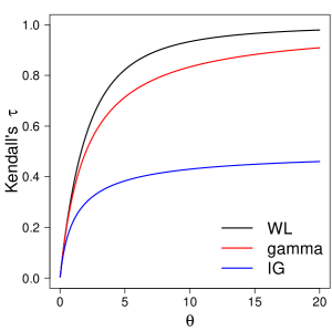
Figure 1: Comparison among Kendall’s $\tau$ for WL frailty, gamma frailty and IG frailty models.

3 ML estimation for the WL frailty model

In this Section, we discuss the parameter estimation for the WL frailty model. First, we discuss an approach based on the assumption of a parametric model for the baseline distribution. Then, we present an EM algorithm to perform the parameter estimation using a non-parametric approach for the baseline distribution.

3.1 Using a parametric approach for the baseline distribution

Let $Y_{ij}$ and $C_{ij}$ be the failure and censoring times for the $j$-th individual in the $i$-th group and $\textbf{x}_{ij}$ be a $p\times 1$ covariate vector (without intercept term), where $1\leq i\leq m$ and $1\leq j\leq n_{i}$. Under a right censoring scheme, we observe the random variables $T_{ij}=\min(Y_{ij},C_{ij})$ and $\delta_{ij}=I(Y_{ij}\leq C_{ij})$, where $I(A)=1$ if the event $A$ occurs (0 otherwise). We assume the frailty terms $Z_{1},\ldots,Z_{m}$ be a random sample from the WL$(\theta$) distribution. Considering the following assumptions:

• The pairs $(Y_{i1},C_{i1}),\ldots,(Y_{in_{i}},C_{in_{i}})$ are conditionally independent given $Z_{i}$, and $Y_{ij}$ and $C_{ij}$ are mutually independent for $j=1,\ldots,n_{i}$.

• $C_{i1},\ldots,C_{in_{i}}$ are non-informative about $Z_{i}$.

Under this setting, the observed log-likelihood function is given by

$$L({\bm{\beta}},\Lambda_{0},\theta) =\prod_{i=1}^{m}\int_{0}^{+\infty}\prod_{j=1}^{n_{i}}\left[z_{i}\lambda_{0}(t_{ij})\exp\left(\textbf{x}_{ij}^{\top}{\bm{\beta}}\right)\right]^{\delta_{ij}}\exp\left(-z_{i}\Lambda_{0}(t_{ij})\textrm{e}^{\textbf{x}_{ij}^{\top}{\bm{\beta}}}\right)f(z_{i};\theta)dz_{i},$$

$$=\left(\frac{\theta a_{\theta}^{-\left(b_{\theta}+1\right)}}{2\Gamma(b_{\theta})}\right)^{m}\exp\left(\sum_{i=1}^{m}\sum_{j=1}^{n_{j}}\delta_{ij}{\bm{x}}_{ij}^{\top}{\bm{\beta}}\right)\prod_{i=1}^{m}\int_{0}^{+\infty}z_{i}^{b_{\theta}^{(i)}-1}(1+z_{i})\textrm{e}^{-z_{i}/a_{\theta}^{(i)}}dz_{i}\prod_{j=1}^{n_{j}}\left[\lambda_{0}(t_{ij})\right]^{\delta_{ij}},$$

$$=\left(\frac{\theta a_{\theta}^{-\left(b_{\theta}+1\right)}}{2\Gamma(b_{\theta})}\right)^{m}\exp\left(\sum_{i=1}^{m}\sum_{j=1}^{n_{j}}\delta_{ij}{\bm{x}}_{ij}^{\top}{\bm{\beta}}\right)\prod_{i=1}^{m}\Gamma\left(b_{\bm{\psi}}^{(i)}\right)\left(a_{\bm{\psi}}^{(i)}\right)^{b_{\bm{\psi}}^{(i)}}\left(1+a_{\bm{\psi}}^{(i)}b_{\bm{\psi}}^{(i)}\right)\prod_{j=1}^{n_{j}}\left[\lambda_{0}(t_{ij})\right]^{\delta_{ij}},$$ (7)

where $a_{\bm{\psi}}^{(i)}=\left(\sum_{j=1}^{n_{i}}\Lambda_{0}(t_{ij})\textrm{e}^{{\bm{x}}_{ij}^{\top}{\bm{\beta}}}+1/a_{\theta}\right)^{-1}$ and $b_{\bm{\psi}}^{(i)}=r_{i}+b_{\theta}$. In a parametric approach, $\Lambda_{0}(t)$ or $\lambda_{0}(t)$ are specified by a set of parameters, say ${\bm{\nu}}$, and then the parameter vector is reduced to $({\bm{\beta}},{\bm{\nu}},\theta)$. For instance, for the Weibull (WEI) distribution we use the parameterization $\Lambda_{0}(t)=\lambda\,t^{\rho}$ and $\lambda_{0}(t)=\lambda\,\rho\,t^{\rho-1}$, where $t>0$ and ${\bm{\nu}}=(\lambda,\rho)\in\mathbb{R}_{+}^{2}$. From a classical approach the ML estimator can be obtained maximizing $\log L({\bm{\beta}},{\bm{\nu}},\theta)$ in relation to ${\bm{\beta}},{\bm{\nu}}$ and $\theta$.

3.2 ML estimation via EM-algorithm and a semiparametric approach

In this subsection, we discuss an EM-type algorithm to perform the parameter estimation for the WL frailty model. Despite this approach can also be used for a parametric approach, the motivation to this development arises from the application of a non-parametric approach to the failure times.

For our particular problem, the complete data are given by ${\bm{D}}_{c}=({\bm{t}}^{\top},{\bm{\delta}}^{\top},\textbf{X}^{\top},{\bm{Z}}^{\top})$, where ${\bm{t}}^{\top}=(t_{11},\ldots,t_{mn_{m}})$, ${\bm{\delta}}^{\top}=(\delta_{11},\ldots,\delta_{mn_{m}})$, $\textbf{X}^{\top}=(x_{11},\ldots,x_{mn_{m}})$ and ${\bm{Z}}^{\top}=(Z_{1},\ldots,Z_{m})$. In our context, ${\bm{D}}_{obs}=\left({\bm{t}}^{\top},{\bm{\delta}}^{\top},\textbf{X}^{\top}\right)$ represents the observed data and ${\bm{Z}}$ (the frailty terms) denotes the latent variables. The complete likelihood function can be written conveniently as $L({\bm{\beta}},{\bm{\Lambda}}_{0},\theta;{\bm{D}}_{c})=L_{1}({\bm{\beta}},\Lambda_{0};{\bm{D}}_{c})\times L_{2}(\theta;{\bm{Z}})$, where $L_{1}({\bm{\beta}},\Lambda_{0};{\bm{D}}_{c})=\prod_{i=1}^{m}\prod_{j=1}^{n_{i}}\left[z_{i}\lambda_{0}(t_{ij})\exp(\textbf{x}_{ij}^{\top}{\bm{\beta}})\right]^{\delta_{ij}}\exp(-z_{i}\Lambda_{0}(t_{ij})\textrm{e}^{\textbf{x}_{ij}^{\top}{\bm{\beta}}})$ and $L_{2}(\theta;{\bm{Z}})=\prod_{i=1}^{m}f(z_{i};\theta)$.
The complete log-likelihood function is given by $\ell_{c}({\bm{\beta}},{\bm{\Lambda}}_{0},\theta;{\bm{D}}_{c})=\ell_{1c}({\bm{\beta}},{\bm{\Lambda}}_{0};{\bm{D}}_{c})+\ell_{2c}(\theta;{\bm{Z}})$, where

$$\ell_{1c}({\bm{\beta}},{\bm{\Lambda}}_{0};{\bm{D}}_{c}) =\sum_{i=1}^{m}\sum_{j=1}^{n_{i}}\left[\delta_{ij}\left(\textbf{x}_{ij}^{\top}{\bm{\beta}}+\log\lambda_{0}(t_{ij})\right)-Z_{i}\Lambda_{0}(t_{ij})\textrm{e}^{\textbf{x}_{ij}^{\top}{\bm{\beta}}}\right]$$

$$\ell_{2c}(\theta;{\bm{Z}}) =m\left[\log(\theta)-\log\Gamma(b_{\theta})-(b_{\theta}+1)\log(a_{\theta})\right]-(b_{\theta}-1)\sum_{i=1}^{m}\log(Z_{i})-\frac{1}{a_{\theta}}\sum_{i=1}^{m}Z_{i}.$$

Let ${\bm{\psi}}^{(\ell)}=({\bm{\beta}}^{(\ell)},\Lambda_{0}^{(\ell)},\theta^{(\ell)})$ be the estimate of ${\bm{\psi}}$ at the $\ell$-th iteration and denote $Q({\bm{\psi}}\mid{\bm{\psi}}^{(\ell)})$ as the conditional expectation of $\ell_{c}({\bm{\psi}})$ given the observed data and ${\bm{\psi}}^{(\ell)}$. With these notations, we have that $Q({\bm{\psi}}\mid{\bm{\psi}}^{(\ell)})=Q_{1}(({\bm{\beta}},\Lambda_{0})\mid{\bm{\psi}}^{(\ell)})+Q_{2}(\theta\mid{\bm{\psi}}^{(\ell)})$, where

$$Q_{1}(({\bm{\beta}},\Lambda_{0})\mid{\bm{\psi}}^{(\ell)}) =\sum_{i=1}^{m}\sum_{j=1}^{n_{i}}\left[\delta_{ij}\left(\textbf{x}_{ij}^{\top}{\bm{\beta}}+\log[\lambda_{0}(t_{ij})\right)]-\widehat{z}_{i}^{(\ell)}\Lambda_{0}(t_{ij})\textrm{e}^{\textbf{x}_{ij}^{\top}{\bm{\beta}}}\right]$$

$$Q_{2}(\theta\mid{\bm{\psi}}^{(\ell)}) =m\left[\log(\theta)-\log\Gamma(b_{\theta})-(b_{\theta}+1)\log(a_{\theta})\right]-(b_{\theta}-1)\sum_{i=1}^{m}\widehat{\kappa}_{i}^{(\ell)}-\frac{1}{a_{\theta}}\sum_{i=1}^{m}\widehat{z}_{i}^{(\ell)},$$

where $\widehat{z}^{(\ell)}_{i}=E(Z_{i}\mid{\bm{D}}_{obs},{\bm{\psi}}={\bm{\psi}}^{(\ell)})$ and $\widehat{\kappa}^{(\ell)}_{i}=E(\log(Z_{i})\mid{\bm{D}}_{obs},{\bm{\psi}}={\bm{\psi}}^{(\ell)})$. It is possible to show that $Z_{i}\mid t_{i1},\ldots,t_{in_{i}},\delta_{i1},\ldots,\delta_{in_{i}}\sim WL\left(\left[a_{\bm{\psi}}^{(i)}\right]^{-1},b_{\bm{\psi}}^{(i)}\right)$. Therefore, using the results presented in Section 2.1 it is immediate that for $i=1,\ldots,m$,

$$\widehat{z}_{i}^{(\ell)} =\frac{b_{\widehat{\bm{\psi}}^{(\ell)}}^{(i)}\left(\left[a_{\widehat{\bm{\psi}}^{(\ell)}}^{(i)}\right]^{-1}+b_{\widehat{\bm{\psi}}^{(\ell)}}^{(i)}+1\right)}{\left[a_{\widehat{\bm{\psi}}^{(\ell)}}^{(i)}\right]^{-1}\left(\left[a_{\widehat{\bm{\psi}}^{(\ell)}}^{(i)}\right]^{-1}+b_{\widehat{\bm{\psi}}^{(\ell)}}^{(i)}\right)},\qquad\mbox{and}$$ (8)

$$\widehat{\kappa}_{i}^{(\ell)} =-\frac{\left[a_{\widehat{\bm{\psi}}^{(\ell)}}^{(i)}\right]^{-1}}{b_{\widehat{\bm{\psi}}^{(\ell)}}^{(i)}\left(\left[a_{\widehat{\bm{\psi}}^{(\ell)}}^{(i)}\right]^{-1}+b^{(i)}_{\widehat{\bm{\psi}}^{(\ell)}}\right)}+\Psi\left(b^{(i)}_{\widehat{\bm{\psi}}^{(\ell)}}+1\right)+\log\left[a^{(i)}_{\widehat{\bm{\psi}}^{(\ell)}}\right].$$ (9)

On the other hand, using the traditional development of the Cox model, it is possible to construct a discrete version of the cumulative baseline hazard function, replacing $\Lambda_{0}(t)$ by $\Lambda_{0}^{D}(t)=\sum_{k:t_{(k)}\leq t}\lambda_{0}(t_{(k)})$, where $t_{(1)},\ldots,t_{(q)}$ denotes the ordered distinct failure times $t_{ij}^{\prime}s$ and $q$ is the number of different observed failure times. With this, the $Q_{1}$ function is given by

$$Q_{1}(({\bm{\beta}},\Lambda_{0})\mid{\bm{\psi}}^{(\ell)}) =\sum_{k=1}^{q}d_{(k)}\log\left[\lambda_{0}(t_{(k)})\right]+\sum_{i=1}^{m}\sum_{j=1}^{n_{i}}\delta_{ij}\textbf{x}_{ij}^{\top}{\bm{\beta}}-\sum_{k=1}^{q}\lambda_{0}(t_{(k)})\sum_{i,j\in R(t_{(k)})}\widehat{z}_{i}^{(\ell)}\textrm{e}^{\textbf{x}_{ij}^{\top}{\bm{\beta}}},$$

where $R(t_{(k)})=\{(i,j):t_{ij}>t_{(k)}\}$ are the observations in risk at the time $t_{(k)}$ and $d_{(k)}$ denotes the number of failures at $t_{(k)}$, for $k=1,\ldots,q$. Note that the solution for $\lambda_{0}(t_{(k)})$ is given by

$$\widehat{\lambda_{0}}(t_{(k)})=\frac{d_{(k)}}{\sum_{i,j\in R(t_{(k)})}\exp\left(\textbf{x}_{ij}^{\top}{\bm{\beta}}+\log\widehat{z}^{(\ell)}_{i}\right)}.$$

With this result, the expression for $Q_{1}$ is reduced to

$$Q_{1}(({\bm{\beta}},\Lambda_{0})\mid{\bm{\psi}}^{(\ell)}) =-\sum_{k=1}^{q}d_{(k)}\log\left(\sum_{i,j\in R(t_{(k)})}\exp\left(\textbf{x}_{ij}^{\top}{\bm{\beta}}+\log\widehat{z}_{i}^{(\ell)}\right)\right)+\sum_{i=1}^{m}\sum_{j=1}^{n_{i}}\delta_{ij}\textbf{x}_{ij}^{\top}{\bm{\beta}}.$$

Note that $Q_{1}(\cdot)$ has the same form of the partial log-likelihood function of the Cox model, except for the offset $\log\widehat{z}_{i}^{(\ell)}$. For this, to update ${\bm{\beta}}$ in the M-step we can use the Cox approach. Finally, the non-parametric estimator for $\Lambda_{0}(\cdot)$ in the $\ell$-th step of the algorithm is given by

$$\widehat{\Lambda}^{(\ell)}_{0}(t)=\sum_{k:t_{(k)}\leq t}\frac{d_{(k)}}{\sum_{i,j\in R(t_{(k)})}\exp\left(\textbf{x}_{ij}^{\top}\widehat{\bm{\beta}}^{(\ell)}+\log\widehat{z}^{(\ell)}_{i}\right)},\quad t>0.$$

In short, the EM algorithm is summarized as follows

• E-step: For $i=1,\ldots,m$, update $\widehat{z}_{i}^{(\ell+1)}$ and $\widehat{\kappa}_{i}^{(\ell+1)}$ using Equations (8) and (9) with $\widehat{\bm{\beta}}^{(\ell)}$, $\widehat{\Lambda}^{(\ell)}_{0}(\cdot)$ and $\widehat{\theta}^{(\ell)}$, the parameters at the $\ell$-th iteration.

• M1-step: Update $\widehat{\bm{\beta}}^{(\ell+1)}$ and $\Lambda_{0}^{(\ell+1)}(\cdot)$ by fitting a Cox regression model with offset $\log\widehat{z}_{i}^{(\ell+1)}$.

• M2-step: Update $\widehat{\theta}^{(\ell+1)}$ by maximizing $Q_{2}(\theta\mid{\bm{\psi}}^{(\ell)})$ in relation to $\theta$.

The E-, M1- and M2-steps are iterated until a convergence criterion is satisfied. For instance, we consider $\left|\left(\widehat{\bm{\beta}}^{(\ell+1)},\widehat{\theta}^{(\ell+1)}\right)-\left(\widehat{\bm{\beta}}^{(\ell)},\widehat{\theta}^{(\ell)}\right)\right|<\epsilon$, where $\epsilon$ is a predefined value. Initial values $\widehat{\bm{\beta}}^{(0)}$ and $\widehat{\Lambda}_{0}^{(0)}(\cdot)$ can be obtained based on the usual Cox regression model. In addition, it is possible to fix $\widehat{z}_{i}^{(0)}=1$ and $\widehat{\kappa}_{i}^{(0)}=0$, for $i=1,\ldots,m$, and an arbitrary value for $\theta$. For instance, we use $\widehat{\theta}^{(0)}=0.5$. Standard errors for $\widehat{\bm{\beta}}$ and $\widehat{\theta}$ can be obtained following the suggestion of Klein (1992). For this, it is considered a profile log-likelihood function, say $\ell({\bm{\beta}},\theta)$, replacing $\Lambda_{0}$ by its estimation $\widehat{\Lambda}_{0}$ and taking the logarithm in Equation (7). Therefore, the information matrix is computed as $I({\bm{\beta}},\theta)=-\partial^{2}\ell({\bm{\beta}},\theta)/\partial\left({\bm{\beta}},\theta\right)\partial^{\top}\left({\bm{\beta}},\theta\right)$. The variance of the ML estimators, say $\widehat{\bm{\beta}}$ and $\widehat{\theta}$, can be estimated numerically. For simplicity’s sake, we omit such details.

Remark 3.1

We also implement an EM-type algorithm when the WEI distribution is assumed as the baseline model. In this case, the EM algorithm is essentially the same. However, instead of a Cox regression model, we need to perform a WEI regression model in the M1-step, but considering the $\log\left(\widehat{z}_{i}^{(\ell)}\right)$ as offset. We implement this using the function survfit included in the package survival (Therneau, 2021) of R Core Team (2022).

Remark 3.2

The package extrafrail (Gallardo and Bourguignon, 2022) of R Core Team (2022) included the computational implementation for the WL frailty model considering as baseline model the WEI distribution and the semi-parametric specification. For instance, to fit the non-parametric case, it can be used

frailtyWL(formula, data, dist = "np")

where as is usually in survival analysis with random effects in R, formula can defined as

Surv(time, event) ~ covariates + cluster(id)

A similar syntax can be used to fit the Weibull case specifying dist="weibull" in last sentence.

4 Simulation study

In this Section we present two simulation studies related to the WL frailty model with a semiparametric baseline. The first study is devoted to study the recovery parameters under different scenarios and the second study assesses the performance of the model with a misspecification in the frailty distribution.

4.1 Recovery parameters

In this subsection, we study the properties of the ML estimators in finite samples obtained using the EM algorithm discussed in subsection 3.2. The data were drawn from a similar scenery than the application. We considered $\Lambda_{0}(t)=\lambda\,t^{\rho}$, i.e., the Weibull distribution. We fixed three cases: i) mean $\mu_{w}=8.6$ and variance $\sigma_{w}^{2}=230$, which implies $\lambda\approx 5.6976$ and $\rho\approx 0.5985$; ii) $\mu_{w}=6.0$ and $\sigma_{w}^{2}=230$, resulting in $\lambda\approx 2.5319$ and $\rho\approx 0.4593$ and; iii) $\mu_{w}=8.6$ and $\sigma_{w}^{2}=100$, resulting in $\lambda\approx 7.9786$ and $\rho\approx 0.8630$. For the clusters, we assumed three scenarios.

• Case 1. $m=396$ clusters with the following distribution: 200 clusters with 1 observation, 100 clusters with 2 observations, 50 clusters with 3 observations, 20 clusters with 4 observations, 20 clusters with 5 observations and 6 clusters with 10 observations, totalizing 790 observations.

• Case 2. $m=396$ clusters with the following distribution: 200 clusters with 2 observations, 100 clusters with 4 observations, 50 clusters with 6 observations, 20 clusters with 8 observations, 20 clusters with 10 observations and 6 clusters with 20 observations, totalizing 1,580 observations.

• Case 3. $m=792$ clusters with the following distribution: 400 clusters with 1 observation, 200 clusters with 2 observations, 100 clusters with 3 observations, 40 clusters with 4 observations, 40 clusters with 5 observations and 12 clusters with 10 observations, totalizing 1,580 observations.

Note that we are considering clusters with different number of observations. We also highlight that Case 2 doubles the observations for each cluster (keeping the number of clusters) and Case 3 doubles the number of clusters (keeping the number of observations for each cluster). Frailty terms were drawn from the WL$(\theta)$ model, where three values were used for $\theta:0.1,0.25$ and $0.5$. We assume the multiplicative hazard model in (2) with four covariates, one of them simulated from the categorical distribution with probabilities $(0.4,0.4$ and $0.2)$. The other three covariates were drawn from the Bernoulli distribution with success probabilities of $0.7$, $0.6$ and $0.5$, respectively. Therefore, for each individual the covariate vector is $\bf{x}_{i}^{\top}=(x_{11i},x_{12i},x_{2i},x_{3i},x_{4i})$. For each case, we consider ${\bm{\beta}}=(\beta_{11},\beta_{12},\beta_{2},\beta_{3},\beta_{4})=(0.3,1.1,0.4,-0.5,-0.3)$. We also consider three percentages of censoring data: 0%, 10% and 25%. With this scheme and defining $\xi_{i}=\bf{x}_{i}^{\top}{\bm{\beta}}$, we obtain

$$\Lambda_{0}(t\mid z_{i},{\bf{x}}_{i})=\lambda\,z_{i}\,\textrm{e}^{\xi_{i}}t^{\rho},$$

i.e., $t\mid z_{i},\bf{x}_{i}$ has Weibull distribution with parameters $\lambda_{i}^{*}=\lambda\,z_{i}\,\textrm{e}^{\xi_{i}}$ and $\rho^{*}=\rho$, where it is simple to draw values. In order to obtain a $100\times q$% of censoring times, we fix $C_{i}$ (the censoring times) as the $100\times(1-q)$-th percentile of the last referred Weibull distribution, so that $P(T_{i}>C_{i})=q$, as requested. For each of the 81 combinations of $(\mu_{2},\sigma_{w}^{2})$, clusters, $\theta$ and censoring, we draw 1,000 samples and then, we compute the ML estimators using the EM algorithm implemented in the extrafrail package. Table 1 summarizes the estimated bias (bias), the mean of the estimated standard errors (SE) and the root of the estimated mean squared error (RMSE) for two cases of the 0% censoring. The remaining cases are given as supplementary material. In general terms, for all the cases the bias is acceptable and the terms SE and RMSE are closer, suggesting that the estimated standard errors for all the estimators are well estimated. Results are similar for different combinations of $\mu_{w}$ and $\sigma_{w}^{2}$. We also note that the frailty variance is better estimated when the number of clusters is maintained, but the observations in each cluster is augmented than the case when the observations in each cluster in maintained, but the number of clusters is augmented. In simple words, to estimate the frailty variance is better to have more intra clusters observations than inter clusters, as expected.

Table 1: Estimated bias, SE and RMSE for the shared WL frailty semiparametric model (censoring: 0%).

			$\mu_{w}=8.6,\sigma_{w}^{2}=230$			$\mu_{w}=6.0,\sigma_{w}^{2}=230$			$\mu_{w}=8.6,\sigma_{w}^{2}=100$
$\theta$	$m/n_{j}$	estimator	bias	SE	RMSE	bias	SE	RMSE	bias	SE	RMSE
0.10	case i	$\widehat{\beta}_{11}$	$-$0.0238	0.0761	0.0894	$-$0.0270	0.0761	0.0879	$-$0.0291	0.0754	0.0892
		$\widehat{\beta}_{12}$	$-$0.0114	0.1020	0.1206	$-$0.0149	0.1020	0.1173	$-$0.0205	0.1015	0.1151
		$\widehat{\beta}_{2}$	0.0029	0.0819	0.0826	0.0056	0.0820	0.0798	0.0016	0.0815	0.0815
		$\widehat{\beta}_{3}$	$-$0.0227	0.0749	0.0823	$-$0.0231	0.0749	0.0836	$-$0.0248	0.0744	0.0835
		$\widehat{\beta}_{4}$	0.0214	0.0694	0.0819	0.0239	0.0694	0.0803	0.0192	0.0690	0.0818
		$\widehat{\theta}$	0.0210	0.0379	0.0339	0.0207	0.0382	0.0350	0.0204	0.0361	0.0343
	case ii	$\widehat{\beta}_{11}$	$-$0.0012	0.0538	0.0627	0.0007	0.0538	0.0595	$-$0.0012	0.0534	0.0585
		$\widehat{\beta}_{12}$	0.0229	0.0690	0.0803	0.0281	0.0691	0.0823	0.0281	0.0688	0.0817
		$\widehat{\beta}_{2}$	0.0087	0.0566	0.0583	0.0100	0.0566	0.0571	0.0090	0.0563	0.0582
		$\widehat{\beta}_{3}$	$-$0.0027	0.0520	0.0574	$-$0.0019	0.0521	0.0545	$-$0.0043	0.0515	0.0552
		$\widehat{\beta}_{4}$	$-$0.0010	0.0481	0.0525	$-$0.0019	0.0482	0.0530	0.0008	0.0478	0.0547
		$\widehat{\theta}$	0.0070	0.0236	0.0200	0.0072	0.0237	0.0197	0.0058	0.0228	0.0194
	case iii	$\widehat{\beta}_{11}$	$-$0.0200	0.0553	0.0641	$-$0.0227	0.0553	0.0640	$-$0.0198	0.0548	0.0650
		$\widehat{\beta}_{12}$	0.0148	0.0706	0.0781	0.0162	0.0706	0.0796	0.0150	0.0702	0.0809
		$\widehat{\beta}_{2}$	0.0019	0.0578	0.0579	0.0066	0.0578	0.0582	0.0015	0.0575	0.0613
		$\widehat{\beta}_{3}$	$-$0.0092	0.0529	0.0552	$-$0.0091	0.0529	0.0594	$-$0.0083	0.0525	0.0567
		$\widehat{\beta}_{4}$	0.0000	0.0492	0.0556	0.0052	0.0492	0.0534	0.0035	0.0488	0.0525
		$\widehat{\theta}$	0.0225	0.0266	0.0304	0.0231	0.0268	0.0308	0.0202	0.0254	0.0282
0.25	case i	$\widehat{\beta}_{11}$	$-$0.0216	0.0813	0.0862	$-$0.0215	0.0815	0.0884	$-$0.0178	0.0803	0.0866
		$\widehat{\beta}_{12}$	$-$0.0602	0.1087	0.1257	$-$0.0571	0.1087	0.1321	$-$0.0633	0.1078	0.1287
		$\widehat{\beta}_{2}$	$-$0.0402	0.0881	0.0941	$-$0.0403	0.0882	0.0960	$-$0.0369	0.0871	0.0915
		$\widehat{\beta}_{3}$	0.0459	0.0798	0.0947	0.0508	0.0799	0.0949	0.0483	0.0788	0.0931
		$\widehat{\beta}_{4}$	$-$0.0288	0.0746	0.0821	$-$0.0270	0.0746	0.0812	$-$0.0243	0.0737	0.0807
		$\widehat{\theta}$	$-$0.0208	0.0441	0.0420	$-$0.0198	0.0444	0.0408	$-$0.0266	0.0414	0.0447
	case ii	$\widehat{\beta}_{11}$	0.0152	0.0574	0.0609	0.0138	0.0575	0.0645	0.0143	0.0568	0.0628
		$\widehat{\beta}_{12}$	$-$0.0302	0.0740	0.0834	$-$0.0290	0.0741	0.0830	$-$0.0291	0.0735	0.0839
		$\widehat{\beta}_{2}$	$-$0.0088	0.0602	0.0591	$-$0.0085	0.0603	0.0598	$-$0.0069	0.0597	0.0602
		$\widehat{\beta}_{3}$	0.0079	0.0554	0.0568	0.0069	0.0555	0.0588	0.0077	0.0547	0.0583
		$\widehat{\beta}_{4}$	0.0276	0.0513	0.0625	0.0294	0.0514	0.0617	0.0280	0.0508	0.0616
		$\widehat{\theta}$	0.0014	0.0333	0.0281	0.0005	0.0334	0.0265	$-$0.0026	0.0320	0.0269
	case iii	$\widehat{\beta}_{11}$	$-$0.0164	0.0586	0.0630	$-$0.0146	0.0587	0.0627	$-$0.0133	0.0580	0.0605
		$\widehat{\beta}_{12}$	$-$0.0456	0.0752	0.0907	$-$0.0488	0.0752	0.0921	$-$0.0484	0.0747	0.0907
		$\widehat{\beta}_{2}$	$-$0.0238	0.0613	0.0641	$-$0.0216	0.0614	0.0616	$-$0.0233	0.0609	0.0628
		$\widehat{\beta}_{3}$	$-$0.0037	0.0561	0.0557	0.0009	0.0562	0.0584	0.0000	0.0555	0.0553
		$\widehat{\beta}_{4}$	0.0044	0.0522	0.0552	0.0055	0.0523	0.0561	0.0039	0.0518	0.0531
		$\widehat{\theta}$	$-$0.0282	0.0313	0.0400	$-$0.0279	0.0315	0.0398	$-$0.0310	0.0296	0.0415

4.2 Assessing the baseline distribution

We devote this subsection to assessing the estimation of the baseline distribution when the frailty WL model is used with a non-parametric specification for $\Lambda_{0}(\cdot)$. For this we draw the covariates using the same specification as the last study. The frailty terms were drawn from the WL model with mean 1 and variance equal to $0.1$, $0.25$ and $0.5$. In addition, we also consider three different distributions, implying a misspecification problem for the frailty distribution. We consider $W$ with uniform distribution between 0 and 2; with distribution gamma with shape and rate equal to 1; and with log-normal distribution with location $-\log(2)/2$ and scale $\log(2)$. Those cases imply mean 1 for the distribution and variance $1/3$, $1$ and $1$, respectively. For all the cases, we consider the true baseline coming from the Weibull model with the same three specifications previously used: i) mean $\mu_{w}=8.6$ and variance $\sigma_{w}^{2}=230$; ii) $\mu_{w}=6.0$ and $\sigma_{w}^{2}=230$ and; iii) $\mu_{w}=8.6$ and $\sigma_{w}^{2}=100$. In order to assess the estimation for the non-parametric baseline estimator, we use two measures: mean and median. Theoretical values (well known $\mu_{w}=\lambda\Gamma(1+1/\rho)$ and $\xi_{w}=\lambda[\log(2)]^{1/\rho}$ for mean and median, respectively) are compared with the respective values based on $\widehat{\Lambda}_{0}(\cdot)$. As for positive random variables it is valid that $E(T)=\int_{0}^{\infty}S(t)dt$, we can use the area under curve of $\widehat{S}_{0}(t)=\exp(-\widehat{\Lambda}_{0}(t))$ to estimate the mean of the baseline distribution as

$$\widehat{\mu_{w}} =t_{(1)}+\sum_{i=1}^{k-1}\left(t_{(j+1)}-t_{(j)}\right)\widehat{S}_{0}(t_{(j)}),$$

where $t_{(1)}<t_{(2)}<\cdots<t_{(k)}$ denote the different failure times observed in the sample. On the other hand, to estimate the median of the distribution (say $\widehat{\xi}_{w}$) we use a linear interpolation between $\left(\tau_{k^{*}},\widehat{S}_{0}(\tau_{k^{*}})\right)$ and $\left(\tau_{k^{*}+1},\widehat{S}_{0}(\tau_{k^{*}+1})\right)$, where $k^{*}=\{i\in\{1,\ldots,k\}:\widehat{S}_{0}(t_{i})\leq 0.5\wedge\widehat{S}_{0}(t_{i+1})\geq 0.5\}$. The results are summarized considering the bias (B) and relative bias (RB) with their corresponding standard deviation (say B-SD and RB-SD, respectively) for the three measures, i.e.,

$$\mbox{B}(\varphi) =\sum_{j=1}^{1000}(\widehat{\varphi}_{i}-\varphi),\quad\mbox{RB}(\varphi)=\sum_{j=1}^{1000}\left(\frac{\widehat{\varphi}_{i}-\varphi}{\varphi}\right),$$

$$\mbox{B-SD}(\varphi) =\sum_{j=1}^{1000}(\widehat{\varphi}_{i}-\varphi)^{2}\quad\mbox{and}\quad\mbox{RB-SD}(\varphi)=\sum_{j=1}^{1000}\left(\frac{\widehat{\varphi}_{i}-\varphi}{\varphi}\right)^{2},$$

for $\varphi\in\{\mu_{w},\xi_{w}\}$. Table 2 summarizes the results for the case with 0% of censoring. The cases with 10% and 25% of censoring are presented as supplementary material. Note that when the frailty distribution is well specified, the maximum RB attaches 0.045, 0.207 and 0.387 for $\theta=0.1$, $0.25$ and $0.5$, respectively, for the mean and a similar pattern is obtained for the mean. Therefore, an increment in the frailty variance deteriorates the estimation for the baseline distribution. Specifically, the baseline distribution is overestimated with increasing frailty variance. This overestimation is also illustrated in Figure 2. On the other hand, for the cases where the frailty distribution was misspecified, the RB ranges from 0.223 to 1.552 and therefore, a misspecification in the frailty distribution also helps to overestimate the baseline distribution. Finally, when the distribution is well specified, a decrement in the mean or in the standard deviation of the true baseline distribution reduces the bias of the baseline estimator or at least makes it more homogeneous.

Table 2: Estimated bias for mean, median and standard deviation of the baseline distribution using shared WL frailty semiparametric model (censoring: 0%).

			WL ($\theta=0.1$)				WL ($\theta=0.25$)				WL ($\theta=0.5$)				U ($\theta=0.33$)				gamma ($\theta=1$)				LN ($\theta=1$)
$\mu_{w}-\sigma_{w}^{2}$	m/n	measure	B	B-SD	RB	RB-SD	B	B-SD	RB	RB-SD	B	B-SD	RB	RB-SD	B	B-SD	RB	RB-SD	B	B-SD	RB	RB-SD	B	B-SD	RB	RB-SD
8.6 - 230	case i	$\mu_{w}$	0.139	1.238	0.016	0.144	0.931	1.331	0.108	0.155	2.519	1.547	0.293	0.180	3.444	1.706	0.400	0.198	6.399	2.034	0.744	0.236	3.657	1.731	0.425	0.201
		$\xi_{w}$	0.077	0.496	0.025	0.161	0.137	0.494	0.044	0.160	0.524	0.591	0.170	0.191	1.018	0.659	0.329	0.213	1.639	0.840	0.531	0.272	1.235	0.736	0.400	0.238
	case ii	$\mu_{w}$	0.367	0.851	0.043	0.099	1.419	0.938	0.165	0.109	2.584	1.067	0.300	0.124	2.893	1.113	0.336	0.129	5.689	1.329	0.662	0.155	3.930	1.153	0.457	0.134
		$\xi_{w}$	0.177	0.361	0.057	0.117	0.460	0.403	0.149	0.130	0.742	0.436	0.240	0.141	1.056	0.483	0.342	0.156	1.853	0.603	0.600	0.195	1.407	0.510	0.455	0.165
	case iii	$\mu_{w}$	0.108	0.879	0.013	0.102	0.609	0.957	0.071	0.111	2.721	1.073	0.316	0.125	2.478	1.117	0.288	0.130	9.812	1.631	1.141	0.190	2.846	1.076	0.331	0.125
		$\xi_{w}$	0.090	0.345	0.029	0.112	0.076	0.355	0.025	0.115	0.700	0.425	0.227	0.138	0.684	0.435	0.222	0.141	2.949	0.776	0.955	0.251	0.891	0.442	0.288	0.143
6.0 - 230	case i	$\mu_{w}$	-0.022	1.042	-0.004	0.174	0.748	1.238	0.125	0.206	2.201	1.381	0.367	0.230	3.135	1.534	0.522	0.256	6.001	1.941	1.000	0.324	3.226	1.564	0.538	0.261
		$\xi_{w}$	0.033	0.231	0.029	0.203	0.069	0.260	0.061	0.228	0.250	0.290	0.219	0.254	0.516	0.342	0.452	0.300	0.851	0.470	0.746	0.413	0.631	0.383	0.553	0.336
	case ii	$\mu_{w}$	0.246	0.751	0.041	0.125	1.241	0.933	0.207	0.156	2.264	0.983	0.377	0.164	2.495	0.985	0.416	0.164	5.252	1.302	0.875	0.217	3.506	1.077	0.584	0.180
		$\xi_{w}$	0.093	0.170	0.082	0.149	0.233	0.208	0.204	0.182	0.368	0.228	0.323	0.200	0.531	0.249	0.466	0.218	0.968	0.349	0.849	0.306	0.730	0.280	0.640	0.246
	case iii	$\mu_{w}$	0.029	0.739	0.005	0.123	0.549	0.812	0.091	0.135	2.320	1.029	0.387	0.172	2.153	0.981	0.359	0.163	9.314	1.582	1.552	0.264	2.519	1.005	0.420	0.168
		$\xi_{w}$	0.050	0.163	0.044	0.143	0.050	0.169	0.043	0.149	0.341	0.218	0.299	0.192	0.335	0.216	0.294	0.190	1.581	0.451	1.387	0.396	0.448	0.236	0.393	0.207
8.6 - 100	case i	$\mu_{w}$	0.167	0.885	0.019	0.103	0.722	0.979	0.084	0.114	1.774	1.108	0.206	0.129	2.632	1.195	0.306	0.139	4.931	1.486	0.573	0.173	2.722	1.179	0.316	0.137
		$\xi_{w}$	0.083	0.568	0.016	0.109	0.159	0.613	0.031	0.117	0.540	0.659	0.104	0.126	1.126	0.703	0.216	0.135	1.846	0.850	0.354	0.163	1.354	0.745	0.259	0.143
	case ii	$\mu_{w}$	0.385	0.628	0.045	0.073	1.155	0.673	0.134	0.078	1.989	0.751	0.231	0.087	2.205	0.783	0.256	0.091	4.258	0.969	0.495	0.113	2.932	0.800	0.341	0.093
		$\xi_{w}$	0.203	0.402	0.039	0.077	0.529	0.441	0.101	0.085	0.866	0.476	0.166	0.091	1.183	0.494	0.227	0.095	2.026	0.609	0.388	0.117	1.556	0.522	0.298	0.100
	case iii	$\mu_{w}$	0.194	0.623	0.023	0.072	0.544	0.681	0.063	0.079	1.975	0.779	0.230	0.091	1.915	0.823	0.223	0.096	7.407	1.173	0.861	0.136	2.159	0.765	0.251	0.089
		$\xi_{w}$	0.098	0.405	0.019	0.078	0.102	0.408	0.020	0.078	0.756	0.484	0.145	0.093	0.800	0.491	0.153	0.094	3.118	0.713	0.598	0.137	0.990	0.483	0.190	0.093

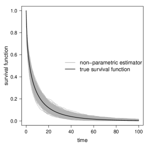
(a) $\theta=0.1$

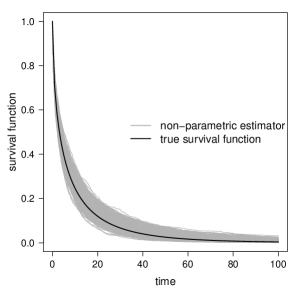
(b) $\theta=0.25$

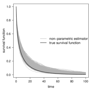
(c) $\theta=0.5$

Figure 2: Non-parametric estimator for the baseline survival function for 1,000 replicates when the data generation and estimation is based on the WL$(\theta$) model with a) $\theta=0.1$, b) $\theta=0.25$ and c) $\theta=0.5$, $\mu_{w}=8.6$, $\sigma_{w}^{2}=230$ and case i) for the specification of the number of clusters/observations in each cluster.

5 Real-world data analysis

In this section, we present an application of the proposed model to real data for illustrative purposes. The data set is related to rehospitalization times after surgery in patients diagnosed with colorectal cancer. It was presented for the first time in González et al. (2005) and it is available in the frailtySurv (Monaco et al., 2018) package of R (R Core Team, 2022). As the times related to a readmission are from the same individual, it is natural to use a frailty model in this context. We consider interocurrence or censoring time (in days) as the response variable. In total, the data contains 861 measures related to 403 patients (mean: 480.01, median: 216, standard deviation: 558.17, 47% of times were censored). The distribution of the observations in each cluster is given in Table 3. Note that an individual (a cluster) has 23 observations.

Table 3: Distribution for the number of observations in each cluster.

Observations in the cluster	1	2	3	4	5	6	7	9	10	11	12	17	23
Number of clusters	199	105	45	21	15	8	4	1	1	1	1	1	1

The considered covariates were: dukes, Dukes’ tumoral stage (A-B: 324, C: 331 and D: 206); charlson, the comorbidity Charlson’s index (0: 577 and 1-2-3: 284); sex (male: 549 and female: 312); and chemo, if the patient received chemotherapy (non-treated: 468 and treated: 393). Figure 3 shows the Kaplan-Meier estimator for the four covariates. Note that apparently the four covariates influence the rehospitalization time.

(a) dukes

(b) charlson

(c) sex

(d) chemo

Figure 3: Kaplan-Meier estimator for the four covariates in readmission data set.

For the analysis, we considered the semi-parametric model with frailty WL, gamma and IG distributions (we refer to such models as semi-WL, semi-gamma and semi-IG, respectively) and the Weibull distribution with frailty WL, gamma and IG distributions (we refer to such models as WEI-WL, WEI-gamma and WEI-IG, respectively). To obtain the estimates for the semi-gamma and semi-IG models, we use the coxph function included in the survival package (Therneau, 2021), where the standard error term is not presented for $\theta$ (the frailty variance) and for the WEI-gamma and WEI-IG we use the parfm function from the parfm package (Munda et al., 2012). Table 5 shows the estimates for such models. We highlight that all the models suggest that the inclusion of the frailty terms is necessary. We also highlight that for the semi-WL and WEI-WL all the estimates for the regression coefficients are significative using a 5%, differently from the other models where the coefficients related to dukesC and chemo were non-significant. On the other hand, the estimated variance for the semi-WL and WEI-WL are very close (0.619 and 0.615, respectively), different to the semi-gamma with WEI-gamma and semi-IG and WEI-IG models, where there is a difference around 15% among the estimated variance using the semi-parametric and the Weibull model. In this line, the WEI-gamma and WEI-IG estimate a greater Kendall’s $\tau$ in comparison with the semi-gamma and semi-IG models, respectively. In this sense, the use of the WL distribution for frailty provides robustness. For this reason, henceforth we consider the analysis with the semi-WL model.

Table 4: Estimation for readmission data set using the semiparametric model and the Weibull model with different frailty distributions: WL, gamma and IG.

	semi-WL			semi-gamma			semi-IG			WEI-WL			WEI-gamma			WEI-IG
Parameter	Estimated		s.e.	Estimated		s.e.	Estimated		s.e.	Estimated		s.e.	Estimated		s.e.	Estimated		s.e.
dukesC	0.308	*	0.121	0.293		0.156	0.294		0.159	0.313	*	0.190	0.293		0.161	0.297		0.165
dukesD	1.125	*	0.170	1.016	*	0.187	1.067	*	0.190	1.110	*	0.213	1.076	*	0.193	1.142	*	0.198
charlson1-2-3	0.420	*	0.119	0.402	*	0.124	0.358	*	0.123	0.372	*	0.121	0.430	*	0.127	0.379	*	0.126
sex	$-$0.578	*	0.127	$-$0.516	*	0.135	$-$0.495	*	0.137	$-$0.495	*	0.145	$-$0.525	*	0.139	$-$0.502	*	0.142
chemo	$-$0.267	*	0.105	$-$0.203		0.138	$-$0.202		0.141	$-$0.284	*	0.169	$-$0.189		0.143	$-$0.188		0.147
$\theta$	0.619		0.123	0.589			0.654			0.615		0.179	0.688		0.142	0.786		0.197
Kendall’s $\tau$	0.246			0.228			0.177			0.245			0.256			0.197
$\rho$										0.440		0.019	0.641		0.026	0.643		0.026
$\lambda$										0.514		0.112	0.449		0.069	0.446		0.070
*Significative coefficients based on a significance level of 5%

Figure 4 shows the estimated frailties for each patient. Note that patients 274 and 318 appear as the patients with a higher risk, whereas patients 80 and 268 appear as the patients with a lower risk. This is corroborated by the descriptive analysis in Table 5. Finally, Figure 5 presents the univariate survival function for one time related to patients 80 and 274 and the marginal survival function for one specific profile.

Figure 4: Estimated frailty terms for each cluster (patient) in readmission data set using the semi-WL model.

Table 5: Descriptive analysis for rehospitalization times for selected patients. $Q_{j}$ denotes the $j$-th quartile.

	Rehospitalization times
Patient	$Q_{1}$	$Q_{2}$	$Q_{3}$	$n_{i}$
80	5.276	5.276	5.276	1
268	5.073	5.073	5.073	1
274	0.006	0.005	0.008	17
318	0.015	0.019	0.041	7
all	0.613	1.565	3.153	2*
*represents the median of the measures for all the patients.

(a)

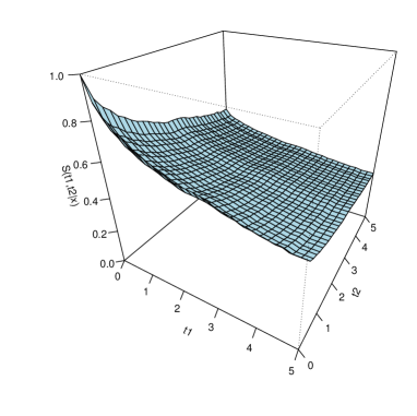
(b)

Figure 5: (a) estimated conditional survival function for one readmission time based on the frailty WL semi-parametric model for patients 80 and 274 and the unconditional survival function for the profile duke=C, charlon=0, sex=female and chemo=treated. (b) Unconditional bivariate survival function based on the semi-WL and the same profile.

6 Concluding remarks

In this paper, we have proposed a novel parametric (the Weibull hazard function was selected as the baseline) and semi-parametric frailty model with WL frailty distribution for modeling unobserved heterogeneity in cluster failure time data, which enjoy mathematical tractability (has a simple Laplace transform) like the gamma frailty model. In particular, the WL distribution with unit mean and variance $\sigma^{2}$ is used as the frailty distribution. The semi-parametric choice of baseline hazard function provides a robust and flexible way to model the data. We get a closed form expression for the derivatives of the Laplace transform for the WL distribution. Furthermore, the conditional distributions of frailties among the survivors and the frailty of individuals dying at time $t$ were determined explicitly. A Monte Carlo simulation study has shown that the estimates based on the EM-algorithm of the model parameters tend to their true values for both parametric and semiparametric cases. In addition, to estimate the frailty variance it is better to perform more intra clusters than inter clusters observations.

Finally, we fitted the proposed regression model to a real dataset on rehospitalization times after surgery in patients diagnosed with colorectal cancer to show the potential of using the new methodology. This application also demonstrates the practical relevance of the new frailty model. From the illustrative example analyzed, the WL frailty model is seen to be quite robust in estimating the covariate effects as well as the frailty variance. Mathematical tractability, flexibility, properties simplicity and computationally attractive of the WL frailty model make the proposed model a competitive one among many models that already exist. In this context, we see that the WL frailty model can also be useful in applications. As part of future research, we plan to explore other estimation methods for the model, including, for instance, the Bayesian approach. Furthermore, the model can be extended to the case of time-varying frailty and the WL frailty model with cure fraction.

Appendix

In this Appendix we detail the proofs related to Propositions 2.2 and 2.3.

6.1 Proof of Proposition 2.2

The conditional density of $Z|T>t$ is

$$f(z|T>t) = \frac{f(z)S(t|z)}{S(t)}$$

$$= \frac{\theta\,a_{\theta}^{-b_{\theta}-1}z^{b_{\theta}-1}(1+z)\exp(-z/a_{\theta})\exp(-z\,\Lambda_{0}(t))}{2\,\Gamma(b_{\theta})[1+a_{\theta}\,H_{0}(t)]^{-b_{\theta}-1}(1+\theta\,\Lambda_{0}(t)/2)}$$

$$= \frac{\theta\,A_{\theta}^{-b_{\theta}-1}z^{b_{\theta}-1}(1+z)\exp(-z/A_{\theta})}{2\,\Gamma(b_{\theta})(1+\theta\,\Lambda_{0}(t)/2)}$$

$$= \frac{A_{\theta}^{-b_{\theta}-1}}{(A_{\theta}^{-1}+b_{\theta})\Gamma(b_{\theta})}z^{b_{\theta}-1}(1+z)\exp(-z/A_{\theta}),\quad{z}>0,$$

where $A_{\theta}=a_{\theta}/(1+a_{\theta}\,\Lambda_{0}(t))$ and $A_{\theta}^{-1}+b_{\theta}=(2+\theta\,\Lambda_{0}(t))/\theta$. This provides that $Z|T>t\sim\textrm{WL}(b_{\theta},A_{\theta}^{-1})$.

6.2 Proof of Proposition 2.3

The conditional density of $Z|T=t$ is given by

$$f(z|T=t) = \frac{f(z)f(t|z)}{f(t)}$$

$$= \frac{\theta\,a_{\theta}^{-b_{\theta}-1}z^{b_{\theta}-1}(1+z)\exp(-z/a_{\theta})z\,\lambda_{0}(t)\,\exp(-z\,\Lambda_{0}(t))}{2\,\Gamma(b_{\theta})\lambda_{0}(t)[1+a_{\theta}\,\Lambda_{0}(t)]^{-b_{\theta}-2}(1+\theta\,\Lambda_{0}(t)/(\theta+2))}$$

$$= \frac{\theta\,a_{\theta}\,A_{\theta}^{-b_{\theta}-2}z^{b_{\theta}}(1+z)\exp(-z/A_{\theta})}{2(\theta+2)^{-1}\,\Gamma(b_{\theta})(\theta+2+\theta\,\Lambda_{0}(t))}$$

$$= \frac{\theta\,A_{\theta}^{-b_{\theta}-2}z^{b_{\theta}}(1+z)\exp(-z/A_{\theta})}{\Gamma(b_{\theta}+1)(\theta+2+\theta\,\Lambda_{0}(t))}$$

$$= \frac{A_{\theta}^{-b_{\theta}-2}}{(A_{\theta}^{-1}+b_{\theta}+1)\Gamma(b_{\theta}+1)}z^{b_{\theta}}(1+z)\exp(-z/A_{\theta}),\quad{z}>0,$$

where $A_{\theta}=a_{\theta}/(1+a_{\theta}\,\Lambda_{0}(t))$, $a_{\theta}b_{\theta}=2/(2+\theta)$ and $A_{\theta}^{-1}+b_{\theta}+1=(\theta+2+\theta\,\Lambda_{0}(t))/\theta$. This provides that $Z|T=t\sim\textrm{WL}(b_{\theta}+1,A_{\theta}^{-1})$.

References

- Abramowitz and Stegun (1972) Abramowitz, M., Stegun, I.A., 1972. Handbook of Mathematical Functions. volume 1. Dover, New York, US.
- Balakrishnan and Liu (2018) Balakrishnan, N., Liu, K., 2018. Semi-parametric likelihood Inference for Birnbaum–Saunders frailty model. REVSTAT 16, 231–255.
- Balakrishnan and Peng (2006) Balakrishnan, N., Peng, Y., 2006. Generalized gamma frailty model. Statistics in Medicine 25, 2797–2816.
- Barreto-Souza and Mayrink (2019) Barreto-Souza, W., Mayrink, V., 2019. Semiparametric generalized exponential frailty model for clustered survival data. Annals of the Institute of Statistical Mathematics 71, 679–701.
- Clayton (1978) Clayton, D., 1978. A model for association in bivariate life tables and its application in epidemiologic studies of familial tendency in chronic disease incidence. Biometrika 65, 141–151.
- Clayton and Cuzick (1985) Clayton, D., Cuzick, J., 1985. Multivariate generalizations of the proportional hazards model. Journal of the Royal Statistical Society, Series A 148, 82–117.
- Congdon (1995) Congdon, P., 1995. Modelling frailty in area mortality. Statistics in Medicine 14, 1859–1874.
- Cox (1972) Cox, D.R., 1972. Regression models and life-tables. Journal of the Royal Statistical Society. Series B (Methodological) 34, 187–220.
- Flinn and Heckman (1982) Flinn, C., Heckman, J., 1982. New methods for analyzing structural models of labor force dynamics. Journal of Econometrics 18, 115–168.
- Gallardo and Bourguignon (2022) Gallardo, D., Bourguignon, M., 2022. A Package for Survival Analysis in R. URL: https://CRAN.R-project.org/package=extrafrail. r package version 1.0.
- Ghitany et al. (2011) Ghitany, M., Alqallaf, F., Al-Mutairi, D., Husain, H., 2011. A two-parameter weighted lindley distribution and its applications to survival data. Mathematics and Computers in Simulation 81, 1190–1201.
- González et al. (2005) González, J., Fernandez, E., Moreno, V., Ribes, J., Peris, M., Navarro, M., Cambray, M., Borràs, J.M., 2005. Sex differences in hospital readmission among colorectal cancer patients. Journal of epidemiology and community health 59, 506–511.
- Hanagal (2019) Hanagal, D., 2019. Modeling Survival Data Using Frailty Models. Springer, Singapore.
- Hougaard (1984) Hougaard, P., 1984. Life table methods for heterogeneous populations. Biometrika 71, 75–83.
- Hougaard (1986a) Hougaard, P., 1986a. A class of multivariate failure time distributions. Biometrika 73, 671–678.
- Hougaard (1986b) Hougaard, P., 1986b. Survival models for heterogeneous populations derived from stable distributions. Biometrika 73, 387–396.
- Klein (1992) Klein, J.P., 1992. Semiparametric estimation of random effects using the cox model based on the em algorithm. Biometrics 48, 795–806.
- Leao et al. (2017) Leao, J., Leiva, V., Saulo, H., Tomazella, V., 2017. Birnbaum–Saunders frailty regression models: Diagnostics and application to medical data. Biometrical journal 59, 291–317.
- Manatunga and Oakes (1999) Manatunga, A., Oakes, D., 1999. Parametric analysis of matched pair survival data. Lifetime Data Analysis 5, 371–387.
- Manton and Vaupel (1986) Manton, K., S.E., Vaupel, J., 1986. Alternative models for heterogeneity of mortality risks among the aged. Journal of the American Statistical Association 81, 635–644.
- Monaco et al. (2018) Monaco, J.V., Gorfine, M., Hsu, L., 2018. General semiparametric shared frailty model: Estimation and simulation with frailtySurv. Journal of Statistical Software 86, 1–42. doi:10.18637/jss.v086.i04.
- Mota et al. (2021) Mota, A., Milani, E., Calsavara, V., Tomazella, V., Leão, J., Ramos, P., Ferreira, P., F., L., 2021. Weighted lindley frailty model: estimation and application to lung cancer data. Lifetime Data Analysis 27, 561–587.
- Munda et al. (2012) Munda, M., Rotolo, F., Legrand, C., 2012. parfm: Parametric frailty models in R. Journal of Statistical Software 51, 1–20. URL: http://www.jstatsoft.org/v51/i11/.
- Piancastelli et al. (2021) Piancastelli, L., Barreto-Souza, W., Mayrink, V., 2021. Generalized inverse-Gaussian frailty models with application to TARGET neuroblastoma data. Annals of the Institute of Statistical Mathematics 73, 979–1010.
- R Core Team (2022) R Core Team, 2022. R: A Language and Environment for Statistical Computing. R Foundation for Statistical Computing. Vienna, Austria. URL: https://www.R-project.org/.
- Therneau (2021) Therneau, T.M., 2021. A Package for Survival Analysis in R. URL: https://CRAN.R-project.org/package=survival. r package version 3.2-11.
- Tyagi et al. (2021) Tyagi, S., Pandey, A., Agiwal, V., Chesneau, C., 2021. Weighted Lindley multiplicative regression frailty models under random censored data. Computational and Applied Mathematics 40, 265.
- Vaupel et al. (1979) Vaupel, J., Manton, K., Stallard, E., 1979. The impact of heterogeneity in individual frailty on the dynamics of mortality. Demography 16, 439–454.
- Wienke (2011) Wienke, A., 2011. Frailty Models in Survival Analysis, publisher = Chapman & Hall, address = Boca Raton, US.