RF Signal Classification with Synthetic Training Data and its Real-World Performance

Abstract

Neural nets are a powerful method for the classification of radio signals in the electromagnetic spectrum. These neural nets are often trained with synthetically generated data due to the lack of diverse and plentiful real RF data. However, it is often unclear how neural nets trained on synthetic data perform in real-world applications. This paper investigates the impact of different RF signal impairments (such as phase, frequency and sample rate offsets, receiver filters, noise and channel models) modeled in synthetic training data with respect to the real-world performance. For that purpose, this paper trains neural nets with various synthetic training datasets with different signal impairments. After training, the neural nets are evaluated against real-world RF data collected by a software defined radio receiver in the field. This approach reveals which modeled signal impairments should be included in carefully designed synthetic datasets. The investigated showcase example can classify RF signals into one of 20 different radio signal types from the shortwave bands. It achieves an accuracy of up to 95% in real-world operation by using carefully designed synthetic training data only.

I Introduction

This paper investigates deep learning for RF signal classification with the application to RF signal identification. Signal identification is the task to identify the type of an unknown wireless signal in the electromagnetic spectrum. The “type” of a signal is sometimes also called transmission mode or service. It is usually defined by some wireless standard with which the waveform is generated (e.g. WiFi, Bluetooth, AM radio broadcast, Stanag 4285, Morse code).

Unlike pure automatic modulation classification (AMC), which extracts only the modulation itself (e.g. PSK, FM, FSK), signal identification also needs to incorporate other characteristic signal parameters such as baud rate, shaping, frame structure or signal envelope to identify the signal type, see Figure 1. Nevertheless, the methods used to solve AMC and signal identification tasks are highly related.

Signal classification is used for spectrum sensing, e.g. to enable dynamic spectrum access in cognitive radio, for spectrum monitoring and signal intelligence applications.

In recent years, machine learning methods like deep neural nets have emerged as a powerful approach to classification problems in the radio domain [1, 2, 3, 4, 5]. Unlike classical algorithm design, which depends on the designers experience and his ability to recognize characteristic signal patterns, machine learning uses large amounts of data to extract meaningful features automatically in a training process.

The challenge of many machine learning approaches is the collection of plenty and diverse training data, which is a requirement for creating powerful systems. The two main types of data are real-world data and synthetic data. Collecting RF training data from a real-world operational scenario often requires a high effort and lacks diversity. This is because the data obtained in a measurement campaign may be specific to the used receiver hardware, current channel conditions and the currently present transmitters. When real data is used, it is often collected in the lab [5, 6, 7] and possibly lacks some real-world effects.

An alternative to real-world data is synthetically generated data. Synthetic data consists of computer-generated waveforms, that are distorted by a channel simulator in software. The channel simulator adds various impairments to the pure signal waveform to model very different reception scenarios, that possibly occur in real-world operation. This impairments can include e.g. frequency offsets, addition of noise or the introduction of fading. The advantage of synthetic data is twofold:

• It can be generated in large amounts

• Diverse signal impairments can be modeled, that lead to robust neural nets, that generalize well.

The main drawback of synthetic training is that it is often unclear how the signals need to be distorted in order to obtain a good classification accuracy in practical operation: Which channel models and effects are important, which are not? How to parameterize the channel simulator in order to obtain realistic, but also diverse data, that ideally models all receiver situations encountered in the real-world application?

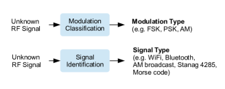
Figure 1: Signal identification vs automatic modulation classification (AMC): AMC outputs only the bare modulation type, whereas signal identification determines exactly the actually sent signal type or mode following some wireless standard.

II Contribution & Related Work

Some papers have investigated the effects of a few isolated channel impairments in synthetic training data, such as frequency offsets [8] or the proper choice of SNR values [9]. However, this covers only a small fraction of the relevant signal impairments. Furthermore, they do not investigate the effects with real-world data. Other works [10, 5] use real-world data for validation, but do not investigate the impact of specific signal impairments in the synthetic dataset.

This paper investigates the influence of synthetic training data on the real-world performance of a signal classifier, thus linking synthetic training with real-world classification performance. For that purpose, several different datasets with varying amount of signal distortion are generated. For each dataset a neural network is trained and evaluated to monitor its performance in a real-world application. Comparing the real-world classification performance reveals the influence of different simulated signal distortions in the training data. In addition, the results provide insight in the generalization ability of the network.

III Training Dataset Generation

III-A Signal Classes

All training datasets contain 20 different signal types, that are shown in Table I. This set includes a large number of digitally modulated signals, such as radioteletype, Navtex, PSK modes, multiple FSK and multi-carrier modes. In addition, different analog modulated signals, such as AM broadcasting, single-sideband (SSB) voice and HF fax are included. These signals are commonly used by commercial, amateur and governmental operators across the shortwave band between 3-30 MHz.

III-B Dataset

A complete dataset contains 120,000 synthetically generated signals for training and another 30,000 for training validation. Each signal consists of 2048 complex IQ samples with a sampling frequency of 6 kHz. This results in a signal duration of approximately 340 ms.

Mode Name	Modulation	Baud Rate
PSK31	PSK	31
PSK63	PSK	63
RTTY 45/170	FSK, 170 Hz shift	45
RTTY 50/450	FSK, 450 Hz shift	50
RTTY 75/170	FSK, 170 Hz shift	75
Navtex / Sitor-B	FSK, 170 Hz shift	100
Olivia 4/500	4-MFSK	125
Olivia 8/250	8-MFSK	31
Olivia 16/500	16-MFSK	31
Olivia 32/1000	32-MFSK	31
Contestia 16/250	16-MFSK	16
MFSK-16	16-MFSK	16
MFSK-32	16-MFSK	31
MFSK-64	16-MFSK	63
MT63 / 500	Multi-Carrier	5
USB (voice)	Single-Sideband (upper)	analog
LSB (voice)	Single-Sideband (lower)	analog
AM broadcast	AM	analog
Morse Code	OOK	variable
HF / Radio Fax	Facsimile	analog

Table I: Signal classes in the datasets

III-C Modeled Effects

An overview of all modeled signal impairments is depicted in Figure 2. In the following the impairments are explained in detail.

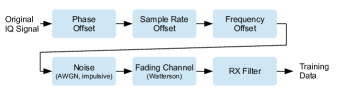
Figure 2: Synthetic dataset generation

III-C1 Phase and Frequency Offset

In general, transmitter and receiver phase and frequency are not synchronized when the signal type is unknown (blind reception). Therefore, a random constant phase shift is added to each signal in the dataset. In addition, a frequency offset is introduced, that is randomly chosen between -250 and +250 Hz to model receiver tuning mismatch.

III-C2 Sample Rate Offset

The sample clock of transmitter and receiver electronics are usually not exactly synchronized. Therefore, a small difference in sample frequencies may be present, that virtually stretches or compresses the signal by a small amount. The generated data uses randomly selected sample frequency offsets of 0, +/-0.5 and +/-1%.

III-C3 Additive Noise

Receiver noise is typically modeled as additive white Gaussian noise (AWGN). However, also other noise types may be present, such as impulsive noise. Impulsive noise often originates from lightnings and other interference in shortwave channels. Thus impulsive noise may sometimes model the noise more accurately. In this paper, impulsive noise is generated by exponentiating the magnitude of ordinary AWGN noise, i.e.

$$n_{impulsive}(t)=sign\left(n_{AWGN}(t)\right)\cdot|n_{AWGN}(t)|^{x}$$

During data generation, the noise type is selected randomly among AWGN and impulsive noise with exponents $x=1.5,2$ or $3$ and added to the signal (see Figure 3).

Proper selection of the noise power ensures that the desired SNR value is achieved. Throughout this paper SNR is referred to the complete Nyquist bandwidth.

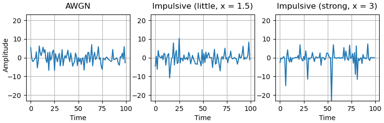
Figure 3: AWGN vs impulsive noise (same noise power)

III-C4 Fading Channels for Shortwave

Time-varying multi-path propagation is present in many communication channels and manifests in fading effects. Fading results in fluctuations of the amplitude of the received signal over time (Figure 4) and frequency (Appendix, Figure 12). At shortwave frequencies, communication mainly occurs through reflections of the electromagnetic waves at the ionosphere. This ionospheric propagation introduces fading and varying Doppler shifts.

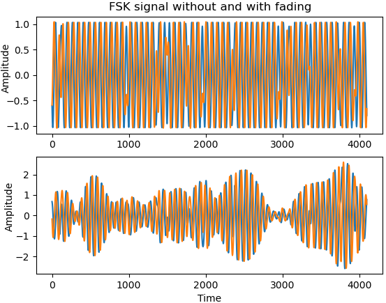
Figure 4: The effect of fading on the amplitude of a RTTY 45/170 IQ signal

The Watterson model [11] is a widely used model for ionospheric propagation and is depicted in Figure 5. It consists of a two-tap delay line, that models two different propagation paths. Each path is multiplied by a independent random noise-like signal, that is frequency filtered such that is introduces random Doppler shifts. In addition, a fixed frequency offset can be introduced in one of the two paths. A concrete realization of the Watterson model is defined by three parameters: differential delay (in ms), Doppler spread (in Hz) and fixed frequency offset (in Hz) (see Figure 5). Different values of these three parameters correspond to different propagation behaviors.

Two standards have been developed, that follow this definition of the Watterson model: CCIR 520 [12] and ITU 1487 [13]. CCIR 520 defines several parameter sets for channels described by their quality (“flat”, “good”, “moderate”, “poor”, “flutter” and “doppler”). ITU 1487 extends the number of parameter sets and introduces channel models for locations at low, medium and high latitudes. Moreover, the parameters of the Watterson model can be set to values that deviate from the standards CCIR and ITU in order to generate more extreme models. This may be useful for training data generation, because additional extreme channel data can improve the generalization capability of the trained network. In summary, this paper investigates three sets of channel models:

• CCIR 520

• ITU 1487

• Extended channel set (CCIR, ITU and extreme models)

Further details on the three sets of fading channel models can be found in the Appendix.

Each signal in the dataset is distorted by a channel model, that is randomly selected from the set of channel models (including the option to use no channel model).

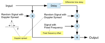
Figure 5: Watterson fading model as used by the HF channel standards CCIR 520 and ITU 1487

III-C5 Receiver Filter (RX Filter)

Signals encountered in practical operation often have varying bandwidths. In the receiver, the operator or an automatic algorithm usually applies a filter, that reduces noise outside the signal bandwidth prior to classification. Therefore a classifier needs to deal with the fact that the noise may not equally be distributed across the complete Nyquist bandwidth as depicted in Figure 6. This effect is modeled in the dataset by applying a bandpass filter. In practice it is not always possible to set a receiver filter exactly to the signal’s bandwidth, e.g. because a signal’s bandwidth is not properly defined or the SNR is very low. Therefore the filter’s bandwidth in the training data varies between the signal bandwidth and the full Nyquist bandwidth in order to train the network on different receiver filter bandwidths.

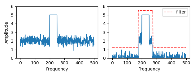
Figure 6: Signal before (left) and after applying a bandpass filter in the receiver (right)

IV Real-World Validation Data

Most scientific works that use synthetic data for training, also use synthetic data of the same distribution for validation (e.g. in [3, 4, 9]). Therefore such ordinary synthetic validation data can only validate the training process and not the final performance in the real application. This paper uses a non-synthetic dataset for validation. It consists of real-world signals, that have been captured “in the field”. This real-world validation data allows to assess the network’s final performance under real-world conditions.

The real-world signals have been obtained using the Twente University WebSDR [14] receiver. The recorded signals are signals of opportunity coincidentally present at reception time in the spectrum. The recorded signals have a high diversity: The signals have been recorded at numerous different SNRs, different times of day and season and different frequencies. This ensures the occurrence of largely different channel conditions (Since channel conditions in the shortwave band are highly dependent on day, season and sun activity). Furthermore, most of the signals were captured from different transmitting stations. This mitigates biasing effects that may originate in emitter specific properties, such as location, transmitter electronics and signal generation.

The receiver filter is roughly set to the signal bandwidth.

All recordings are cut into a collection of data signals with each having a length of 2048 IQ samples (same as training data format). Apart from that, no further change of the signal is made. Thus all signal impairments remain “as they are”.

Table II presents an overview of the recorded data. The total recording time of the real-world signals is in the order of several hours. Since the recorded signal types have different amounts of data, it is important to balance the classes properly in order to get meaningful results.

Mode Name	# Data	SNR Range	Frequencies / Bands
PSK31	3,700	-10 to +25 dB	40 m, 20 m
PSK63	5,500	-10 to +25 dB	80 m, 40 m, 20 m
RTTY 45/170	5,200	-10 to +40 dB	40 m, 20 m
RTTY 50/450	11,300	-10 to +35 dB	4.5 to 11.0 MHz
RTTY 75/170	3,600	-10 to +35 dB	80 m, 40 m, 20 m
Navtex / Sitor-B	9,000	-10 to +20 dB	0.5, 4.2, 8.4, 12.6 MHz
Olivia 4/500	1,300	+5 to +15 dB	80 m
Olivia 8/250	7,600	-10 to +25 dB	80 m to 20 m
Olivia 16/500	4,000	-10 to +20 dB	80 m, 40 m, 20 m
Olivia 32/1000	4,700	-5 to +35 dB	20 m
Contestia 16/250	1,700	-10 to +10 dB	40 m, 20 m
MFSK-16	3,500	-10 to +15 dB	80 m, 40 m, 20 m
MFSK-32	4,000	-10 to +15 dB	19 m, 7.8 MHz
MFSK-64	5,400	-10 to +15 dB	19 m, 7.8 MHz
MT63 / 500	1,300	-10 to +15 dB	40 m
USB (voice)	12,700	-10 to +30 dB	5 to 28 MHz
LSB (voice)	13,100	-10 to +25 dB	3 to 10 MHz
AM broadcast	10,900	-10 to +45 dB	75 m to 16 m
Morse Code	6,300	-10 to +20 dB	80 m to 10 m
HF / Radio Fax	20,100	-10 to +35 dB	3.9 to 13.8 MHz

Table II: Recorded real-world validation data for final evaluation: data from various transmitters has been recorded at different times of day, season, frequency and location

V Training

For the evaluation of the synthetic dataset generation, eleven separate datasets with different properties have been generated. Table III shows an overview of the all datasets. From the top down, each dataset adds an additional signal impairment. The first dataset contains no impairments, whereas the last dataset contains all considered impairments. Note, that the dataset names indicate the signal impairment that has been specifically added to this dataset (see Table III).

Dataset Name	Frequency Offset	Phase Offset	fs Offset	Noise	RX Filter	Fading Channel
No Augmentation	-	-	-	-	-	-
Frequency Offset	+/- 250 Hz	-	-	-	-	-
Phase Offset	+/- 250 Hz	random	-	-	-	-
fs Offset	+/- 250 Hz	random	yes	-	-	-
AWGN, high SNR	+/- 250 Hz	random	yes	AWGN: +5 to +25 dB SNR	-	-
AWGN, full SNR	+/- 250 Hz	random	yes	AWGN: -15 to +25 dB SNR	-	-
Impulsive Noise	+/- 250 Hz	random	yes	AWGN or Impulsive: -15 to +25 dB SNR	-	-
RX Filter	+/- 250 Hz	random	yes	AWGN or Impulsive: -15 to +25 dB SNR	yes	-
CCIR Fading	+/- 250 Hz	random	yes	AWGN or Impulsive: -15 to +25 dB SNR	yes	CCIR 520
ITU Fading	+/- 250 Hz	random	yes	AWGN or Impulsive: -15 to +25 dB SNR	yes	ITU 1487
Extended Fading	+/- 250 Hz	random	yes	AWGN or Impulsive: -15 to +25 dB SNR	yes	Extended

Table III: Analyzed training datasets

The synthetic datasets are used to train the neural network shown in Figure 7. The network is a convolutional neural network (CNN) with 9 layers and approximately 550,000 parameters. The complex IQ input data is fed into the network with real and imaginary part separated into two input channels. The CNN is trained on 120,000 signals using an Adam optimizer and a batch size of 128 for 20 epochs.

After the training is completed, the resulting trained net is finally validated once with the real-world validation dataset to measure its performance in a real-world scenario.

To mitigate statistical effects of the training process, five networks have been trained independently for each dataset and the average accuracy is considered as final result.

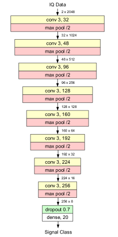
Figure 7: 9-layer CNN used for training

VI Results

VI-A Overall

Figure 8 presents the main results of the paper. It shows the accuracy of the neural networks, each trained by one of the eleven different datasets measured against the real-world dataset. The most sophisticated training datasets achieve an accuracy of 95 % for high SNR values. This demonstrates, that training with carefully designed synthetic data generalizes well to real-world data. Next, the impact of the different channel impairments is investigated in greater detail.

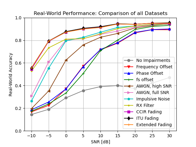
Figure 8: Comparison of the real-world performance for all eleven training datasets

VI-B Impact of Offsets in Frequency, Phase and Sample Rate

Figure 9 focuses on the impact of frequency, phase and sample rate offset. As a first interesting observation, training with clean signals without any impairments works remarkably well and accuracies above 40% can be obtained. Introducing frequency offsets to the training data largely improves accuracy. This is because adding a frequency offset can heavily change the signal shape in the time domain. The introduction of phase offsets has very little impact, showing that the network does not respond to absolute phase. The application of sample rate offsets provides a minor improvement for high SNR at the expense of slightly lower accuracy at smaller SNR.

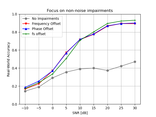
Figure 9: Focus on non-noise effects: frequency, phase and sample rate offset

VI-C Impact of AWGN and Impulsive Noise

The question how noise impacts the final accuracy can be answered with Figure 10. The baseline is the “fs offset” dataset containing the above mentioned non-noise effects, but no noise impairments. The training dataset “AWGN, high SNR” additionally introduces AWGN noise to the data with SNR values between +5 to +25 dB (see Table III). As expected this improves the accuracy above 5 dB SNR. However, it also improves accuracy below 5 dB although low SNR data is not yet included in the training data. This is strong evidence that the network is able to generalize towards lower SNR.

The training dataset “AWGN, full SNR” introduces AWGN noise with a wider SNR range from -15 dB to +25 dB, i.e. it also includes low SNR values. The inclusion of lower SNR values improves the accuracy in the low SNR region below 5 dB as expected. However, also a small increase at SNRs above 5 dB can be observed, which again is evidence that the network improved its generalization capabilities.

The inclusion of impulsive noise showed no major advantage. The accuracy slightly increases for higher SNR and decreases for lower SNR. Although impulsive noise does not provide a clear improvement, it may nevertheless be useful to improve network generalization and robustness.

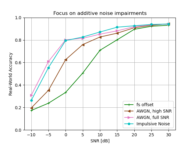
Figure 10: Focus on additive noise effects

VI-D Impact of Fading and RX Filtering

Figure 11 shows the results for training data, that employ receiver (RX) filtering and different fading channels. The inclusion of the filter largely improves the accuracy in the low SNR region. Note, that the reason for this improvement is not simply the reduction of noise in the signal by the filter, because this filtering has been added specifically to the training data. The real-world validation data always includes a more or less tight filter (independent of the training dataset), because RF receivers typically use filters to remove out-of-band noise and interference. Since the impact of the RX filter on the time domain signal is more present for low SNR, the improvement becomes apparent in the low SNR region.

The introduction of fading channels shows a clear increase in accuracy. It shows the importance of applying fading channel models, that model amplitude fluctuations and frequency selective attenuation. Interestingly, all three applied fading channel models (CCIR 520, ITU 1487 and the extended custom set) provide very similar accuracy.

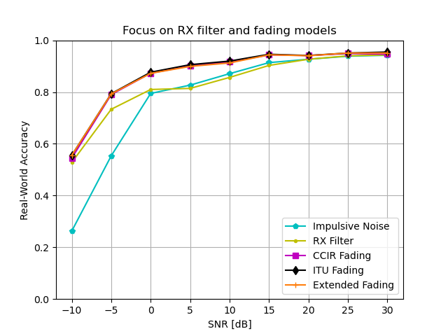
Figure 11: Focus on RX filtering and fading models: CCIR 520, ITU 1487 and “Extended”

VII Conclusion

This paper demonstrated how synthetically generated training data can be used to create radio signal classifiers with high accuracy under real-world operation. It has been investigated how different signal impairments influence the real-world accuracy and the network’s ability to generalize. The results show the importance of training with frequency offsets, a wide range of SNR values and modeling an RX filter and fading channels. The choice of the fading channel was uncritical with regard to the exact channel parameters. Minor to no improvements have been observed for phase offset, sample rate offset and impulsive noise. In the example scenario of 20 RF signal classes, a CNN, trained only by synthetic data, has obtained an accuracy of up to 95 % on real-world signals.

Appendix A Watterson Channel Models

The appendix provides detailed information on the fading channel models used for training data generation. The baseline model is the Watterson model as described in the standards CCIR 520 and ITU 1487 [11, 13, 12]. An concise description of the Watterson model has been provided in Section III-C4.

Tables IV, V and VI provide the exact parametrization of the three investigated channel sets: CCIR 520, ITU 1487 and Extended. Note, that the flat fading channels of CCIR 520 consider only one path. Also note, that some channels from CCIR 520 and ITU 1487 overlap, i.e. they have the same parametrization (e.g. CCIR 520 “good“ and ITU “mid quiet”). For few channels CCIR and ITU do not provide exact parameters but a range of parameters. In these cases either a meaningful value has been selected or two channel models have been considered (e.g. with CCIR 520 “Flat 1” and “Flat 2“).

Figure 12 shows the influence of some fading models on a multi-carrier signal. It visualizes the fluctuations of amplitude over time and frequency.

Channel Name	Paths / Taps	Differential Time Delay	Frequency Spread	Frequency Offset
Flat 1	1	-	0.2 Hz	-
Flat 2	1	-	1 Hz	-
Good	2	0.5 ms	0.1 Hz	-
Moderate	2	1 ms	0.5 Hz	-
Poor	2	2 ms	1 Hz	-
Flutter	2	0.5 ms	10 Hz	-
Doppler	2	0.5 ms	0.2 Hz	5 Hz

Table IV: Channel models defined by standard CCIR 520

Channel Name	Paths / Taps	Differential Time Delay	Frequency Spread	Frequency Offset
Low - Quiet	2	0.5 ms	0.5 Hz	-
Low - Moderate	2	2 ms	1.5 Hz	-
Low - Disturbed	2	6 ms	10 Hz	-
Mid - Quiet	2	0.5 ms	0.1 Hz	-
Mid - Moderate	2	1 ms	0.5 Hz	-
Mid - Disturbed	2	2 ms	1 Hz	-
Mid - NVIS	2	7 ms	1 Hz	-
High - Quiet	2	1 ms	0.5 Hz	-
High - Moderate	2	3 ms	10 Hz	-
High - Disturbed	2	7 ms	30 Hz	-

Table V: Channel models defined by standard ITU 1487

Channel Name	Standard	Paths/ Taps	Differential Time Delay	Frequency Spread	Frequency Offset
Flat 1	CCIR	1	-	0.2 Hz	-
Flat 2	CCIR	1	-	1 Hz	-
Good	CCIR	2	0.5 ms	0.1 Hz	-
Moderate	CCIR	2	1 ms	0.5 Hz	-
Poor	CCIR	2	2 ms	1 Hz	-
Flutter	CCIR	2	0.5 ms	10 Hz	-
Doppler	CCIR	2	0.5 ms	0.2 Hz	5 Hz
Low - Disturbed	ITU	2	6 ms	10 Hz	-
Mid - NVIS	ITU	2	7 ms	1 Hz	-
High - Moderate	ITU	2	3 ms	10 Hz	-
High - Disturbed	ITU	2	7 ms	30 Hz	-
Poor Doppler	-	2	2 ms	1 Hz	10 Hz
High - Moderate Doppler	-	2	3 ms	10 Hz	8 Hz
Extreme 1	-	2	1 ms	40 Hz	-
Extreme 2	-	2	5 ms	0.5 Hz	-

Table VI: Extended channel model set: combination of CCIR, ITU and custom-designed extreme case channels

Figure 12: Example of a multi-carrier signal, that has been modified by some of the considered Watterson channel models (spectrogram representation, time at vertical axis)

References

- [1] L. J. Wong, W. H. Clark, IV, B. Flowers, R. M. Buehrer, A. J. Michaels, and W. C. Headley, “The RFML Ecosystem: A Look at the Unique Challenges of Applying Deep Learning to Radio Frequency Applications.” https://arxiv.org/abs/2010.00432, 2020.
- [2] S. Scholl, “Classification of Radio Signals and HF Transmission Modes with Deep Learning.” https://arxiv.org/abs/1906.04459, 2019.
- [3] P. Wu, B. Sun, S. Su, J. Wei, J. Zhao, X. Wen, and R. Zdunek, “Automatic Modulation Classification Based on Deep Learning for Software-Defined Radio,” Mathematical Problems in Engineering, vol. 2020, p. 2678310, 2020.
- [4] T. O’Shea, J. Corgan, and T. Clancy, “Convolutional Radio Modulation Recognition Networks,” in International Conference on Engineering Applications of Neural Networks, 2016.
- [5] Timothy J. O’Shea, Tamoghna Roy, and T. Charles Clancy, “Over the Air Deep Learning Based Radio Signal Classification,” CoRR, vol. abs/1712.04578, 2017.
- [6] N. Bitar, S. Muhammad, and H. H. Refai, “Wireless technology identification using deep Convolutional Neural Networks,” in 2017 IEEE 28th Annual International Symposium on Personal, Indoor, and Mobile Radio Communications (PIMRC), pp. 1–6, 2017.
- [7] M. Schmidt, D. Block, and U. Meier, “Wireless interference identification with convolutional neural networks,” in IEEE 15th International Conference on Industrial Informatics (INDIN), pp. 180–185, 2017.
- [8] S. C. Hauser, W. C. Headley, and A. J. Michaels, “Signal detection effects on deep neural networks utilizing raw IQ for modulation classification,” in MILCOM 2017 - 2017 IEEE Military Communications Conference (MILCOM), pp. 121–127, 2017.
- [9] Sharan Ramjee, Shengtai Ju, Diyu Yang, Xiaoyu Liu, Aly El Gamal, and Yonina C. Eldar, “Fast Deep Learning for Automatic Modulation Classification.” https://arxiv.org/abs/1901.05850, 2019.
- [10] William H. Clark IV, Steven C. Hauser, William C. Headley, and Alan J. Michaels, “Training Data Augmentation for Deep Learning RF Systems,” CoRR, vol. abs/2010.00178, 2020.
- [11] C. Watterson, J. Juroshek, and W. Bensema, “Experimental Confirmation of an HF Channel Model,” IEEE Transactions on Communication Technology, vol. 18, no. 6, pp. 792–803, 1970.
- [12] CCIR, “RECOMMENDATION F.520-2: USE OF HIGH FREQUENCY IONOSPHERIC CHANNEL SIMULATORS,” 1992.
- [13] ITU-R, “Recommendation ITU-R F.1487: Testing of HF modems with bandwidths of up to about 12 kHz using ionospheric channel simulators,” 05/2000.
- [14] Pieter-Tjerk de Boer, “Wide-band WebSDR.” http://websdr.ewi.utwente.nl:8901/, University of Twente.