-

Constrained Shortest-Path Reformulations for Discrete Bilevel and Robust Optimization

Constrained Shortest-Path Reformulations for Discrete Bilevel and Robust Optimization

Leonardo Lozano Operations, Business Analytics & Information Systems, University of Cincinnati, 2925 Campus Green Drive,
Cincinnati, OH 45221
leolozano@uc.edu

David Bergman Department of Operations and Information Management, University of Connecticut, 2100 Hillside Rd, Storrs, CT 06268
david.bergman@uconn.edu

Andre A. Cire Dept. of Management, University of Toronto Scarborough and Rotman School of Management
Toronto, Ontario M1C 1A4, Canada
andre.cire@rotman.utoronto.ca

Many discrete optimization problems are amenable to constrained shortest-path reformulations in an extended network space, a technique that has been key in convexification, bound strengthening, and search mechanisms for a large array of nonlinear problems. In this paper, we expand this methodology and propose constrained shortest-path models for challenging discrete variants of bilevel and robust optimization, where traditional methods (e.g., dualize-and-combine) are not applicable compared to their continuous counterparts. Specifically, we propose a framework that models problems as decision diagrams and introduces side constraints either as linear inequalities in the underlying polyhedral representation, or as state variables in shortest-path calculations. We show that the first case generalizes a common class of combinatorial bilevel problems where the follower’s decisions are separable with respect to the leader’s decisions. In this setting, the side constraints are indicator functions associated with arc flows, and we leverage polyhedral structure to derive an alternative single-level reformulation of the bilevel problem. The case where side constraints are incorporated as node states, in turn, generalizes classical robust optimization. For this scenario, we leverage network structure to derive an iterative augmenting state-space strategy akin to an L-shaped method. We evaluate both strategies on a bilevel competitive project selection problem and the robust traveling salesperson with time windows, observing considerable improvements in computational efficiency as compared to current state-of-the-art methods in the respective areas.

Integer Programming, Benders Decomposition, Dynamic Programming First submitted on June 7, 2022.

1 Introduction

Given a graph $G$ equipped with arc lengths, the constrained shortest-path problem (CSP) asks for the shortest path between two vertices of $G$ that satisfies one or more side constraints, such as general arc-based budget restrictions or limits on the number of nodes traversed. CSPs are fundamental models in the operations literature, with direct applications both in practical transportation problems (Festa 2015), as well as in a large array of solution methodologies for routing and multiobjective optimization (Irnich and Desaulniers 2005). Due to its importance, the study of scalable algorithms for CSPs and related problems is an active and large area of research (e.g., Cabrera et al. 2020, Vera et al. 2021, Kergosien et al. 2022).

In this paper, we expand upon this concept and propose the use of CSPs as a modeling construct for more general classes of optimization problems. Our approach consists of reformulating either a relaxation or a projection of the problem in an extended compact network space, where paths of the network have a one-to-one relationship to potential feasible solutions of the system. Solving such a relaxation or projection then reduces to finding a constrained shortest path, where side constraints incorporate information of the missing constraints or variables of the original problem. In particular, we exploit network reformulations based on decision diagrams (Bergman et al. 2016), which are compressed networks obtained from the state-transition graph of recursive models.

The distinct attribute of this approach is that one can leverage network structure to derive new reformulations and more efficient algorithm classes, which provide a novel “combinatorial” perspective to such problems when the framework is applicable. More precisely, we exploit the dual description of a constrained shortest-path problem as either a network-flow model (i.e., its polyhedral perspective), or as a label-setting search (i.e., its dynamic programming perspective), applying each based on the setting at hand and the information captured by the side constraints.

Specifically, in this work we focus and illustrate the modeling construct on two classes of optimization problems. The first refer to binary bilevel programs of the form

$$\max_{x^{L},x^{F}\in\{0,1\}^{n}}\bigg{\{}c_{1}^{L}x^{L}+c_{2}^{L}x^{F}\colon A^{L}x^{L}+B^{L}x^{F}\leq b^{L},x^{F}\in\argmax_{\overline{x}^{F}\in\{0,1\}}\left\{c^{F}\overline{x}^{F}\colon A^{F}\,\overline{x}^{F}\leq b^{F},\overline{x}^{F}\leq\mathbf{1}-x^{L}\right\}\bigg{\}},$$

where variables $x^{F}$ and $x^{L}$ formulate a leader’s and a follower’s decisions, respectively. The model above is prevalent in network interdiction problems (Morton et al. 2007, Cappanera and Scaparra 2011, Hemmati et al. 2014, Lozano and Smith 2017a), minimum edge and vertex blocker problems (Bazgan et al. 2011, Pajouh et al. 2014), and other classes of adversarial settings (Costa et al. 2011, Caprara et al. 2016, Zare et al. 2018). However, its challenge stems from the possibly difficult combinatorial structure associated with the follower’s variables, often preventing direct extensions of duality-based solution methodologies from continuous bilevel programs.

We show that, alternatively, the follower’s subproblem can be formulated as a CSP, with univariate side constraints parameterized by the leader’s variables $x^{L}$. In particular, the coefficient matrix of the CSP has a totally unimodular structure and, thus, allows typical polyhedral approaches (i.e., dualize-and-combine) to rewrite the “argmax” of the follower’s problem as a feasibility system. Further, we also exploit the property of the duals of the follower’s network reformulation to convexify non-linear inequalities associated with this model, which appear due to complementary slackness constraints derived from the dualize-and-combine technique. The resulting model is an extended, single-level mixed-integer linear programming (MILP) reformulation of the original bilevel problem, and thus amenable to commercial state-of-the-art solvers.

The second problem class we investigate is robust optimization,

$$\min_{x\in\{0,1\}}\left\{cx\colon A(\delta)\,x\leq b(\delta),\,\forall\delta\in\Delta\right\}.$$

where $\Delta$ is a uncertainty set that parameterizes the realizations of the coefficient matrix $A(\delta)$ and right-hand side $b(\delta)$. Problems of this form have been investigated extensively, with existing approaches primarily based on cutting-plane algorithms akin to Benders decomposition (Mutapcic and Boyd 2009, Zeng and Zhao 2013, Ben-Tal et al. 2015, Ho-Nguyen and Kılınç-Karzan 2018, Borrero and Lozano 2021). Each step in such procedures involves solving an MILP of increasing size, which may often inhbit the scalability of the approach.

We demonstrate that the robust problem can be reformulated as a CSP where side constraints are parameterized by elements $\delta$ of the uncertainty set $\Delta$. The resulting model, however, can be (potentially infinitely) large. We propose a methodology that starts with a smaller subset $\Delta^{\prime}\subset\Delta$ and encode the resulting CSP problem as a dynamic program, thereby amenable to scalable combinatorial CSP labeling algorithms (Cabrera et al. 2020, Vera et al. 2021). Violated constraints are then identified through a separation oracle to augment $\Delta^{\prime}$, and the procedure is repeated. Thus, the procedure is akin to a cutting-plane method, but where labels in the CSP play the role of Benders cuts in the proposed state-augmenting procedure.

We evaluate the bilevel and robust methodologies numerically on case studies in competitive project selection and the robust traveling salesperson problem, respectively. For the bilevel case, we compare the proposed single-level reformulation with respect to a state-of-the-art generic bilevel solver based on branch-and-cut (Fischetti et al. 2017). Results suggest that, even for large networks and using default solver settings, our methodology provides considerable solution time improvements with respect to the branch-and-cut bilevel solver. For the robust case, we compare our method with respect to an MILP-based cutting plane method. We observed similar compelling improvement, where gains were primarily obtained when solving the CSP via an existing labeling method (Lozano and Medaglia 2013) as opposed to a linear formulation with integer programming.

Contributions. Our primary contribution is the structural and numerical development of a CSP-based reduction methodology, specifically focusing on challenging classes of binary bilevel programs and robust optimization. We show that one can either exploit network flows models or dynamic programming to obtain, respectively, extended mixed-integer linear formulations or algorithms that are built on constant-evolving solvers. Our secondary contributions refer to the development of numerical methods to an important class of bilevel programming and robust optimization, which in our experiments have suggested large runtime improvements when sufficiently compact networks for the underlying combinatorial problem sizes are available. We also discuss generalizations of the framework for other classes of bilevel and robust problems.

Paper organization. The remainder of this paper is organized as follows. Section 2 presents a literature review on related algorithms. In Section 3, we briefly review reformulations of discrete optimization problems as network models, more specifically decision diagrams. Section 4 formalizes the description of our proposed constrained path formulations over decision diagrams. Section 5 implements the approach for a class of discrete bilevel programs and depicts an application on competitive project selection. Section 6 considers the approach for classical robust optimization with an application to the robust traveling salesperson problem with time windows. Finally, Section 7 concludes the manuscript and articulate future directions. For the sake of conciseness, we include in the main body of the manuscript the proofs for selected propositions and the remaining proofs are included in the appendices.

2 Related Work

Constrained shortest-path problems (CSP) define an extensive literature in both operations and the computer science literature. We refer to the survey by Festa (2015) for examples of techniques and applications. In particular, the closest variant to our work refers to the shortest-path with resource constraints (SPPRC), first proposed by Desrosiers (1986) and widely investigated as a pricing model in column-generation approaches (Irnich and Desaulniers 2005). The classic SPPRC views constraints as limited “resources” that accumulate linearly over arcs as a path is traversed. Our work considers equivalent resource constraints over graph-based reformulations of general discrete optimization, specifically via decision diagrams in our context.

We consider two CSP models that serve as the basis of our reformulations. The first is a mathematical program derived from a polyhedral representation of shortest-path problems over decision diagrams. This perspective is akin to classical network extended formulations based on dynamic programming (e.g., Eppen and Martin 1987, Conforti et al. 2010, de Lima et al. 2022) with applications to cut-generation procedures (Davarnia and Van Hoeve 2020, Castro et al. 2021), discrete relaxations (van Hoeve 2022), convexification of nonlinear constraints (Bergman and Cire 2018, Bergman and Lozano 2021), and reformulations of big-M constraints in routing problems (Cire et al. 2019, Castro et al. 2020).

The second CSP model we consider is based on dynamic programming (DP) and related models, which have been used extensively in state-of-the-art techniques for large-scale CSPs (e.g., Dumitrescu and Boland 2003, Cabrera et al. 2020, Vera et al. 2021). In general, the DP in this context solves a shortest-path problem on an extended graph via a specialized recursion that labels the states achievable at a node. The benefit of such models is that they do not require linearity and exploit the combinatorial structure of the graph for efficiency. We expand on such models in §4 and refer to Irnich and Desaulniers (2005) for general survey of labeling algorithms for CSPs.

Our first main contribution is a reformulation of a discrete class of bilevel optimization problems. Bilevel optimization is an active research field with applications in energy and natural gas market regulation (Dempe et al. 2011, Kalashnikov et al. 2010), waste management (Xu and Wei 2012), bioengineering (Burgard et al. 2003), and traffic systems (Brotcorne et al. 2001, Dempe and Zemkoho 2012), to name a few. Variants where the follower’s problem is convex are solved by a dualize-and-combine approach, which combines the Karush-Kuhn-Tucker (KKT) optimality conditions of the follower’s problem with the leader’s model. This results in a single-level nonlinear reformulation approachable by a wide array of convexification and other specialized approaches; we refer to the survey by Dempe et al. (2015), Kleinert et al. (2021) for further details and applications.

The dualize-and-combine approach, however, is not generally applicable for cases where decision variables are discrete. An important special case refers to the large class of interdiction problems, where the leader and follower play an adversarial relationship (see, e.g., survey by Smith and Song 2020). Discrete bilevel problems are generally challenging and have fostered a large array of methodologies that extended their single-level counterpart. Solution approaches include branch and bound (DeNegre and Ralphs 2009, Xu and Wang 2014), Benders decomposition (Saharidis and Ierapetritou 2009), parametric programming (Domínguez and Pistikopoulos 2010), column-and-rown generation (Baggio et al. 2021), and cutting-plane approaches based on an optimal value-function reformulations (Mitsos 2010, Lozano and Smith 2017b). In particular, the state-of-the-art approach for mixed-integer linear bilevel programs is the branch-and-cut algorithm by Fischetti et al. (2017), which we use as a benchmarck algorithm in our computational experiments. In contrast to such literature, our method is a dualize-and-combine technique that is applicable when the leader wishes to “block” the follower’s decisions. We exploit the structure of the decision diagram to provide a linear optimality certificate for the follower’s problem, which leads to an alternate single-level reformulation that is amenable to classical mathematical programming solvers.

Our second contribution is an approach to address discrete robust optimization problems via CSP reformulations. Robust optimization is also pervasive in optimization, with extensive literature in both theory (Bertsimas et al. 2004, Ben-Tal et al. 2006, Bertsimas and Brown 2009, Li et al. 2011, Bertsimas et al. 2016) and applications (Lin et al. 2004, Ben-Tal et al. 2005, Bertsimas and Thiele 2006, Yao et al. 2009, Ben-Tal et al. 2011, Gregory et al. 2011, Moon and Yao 2011, Gorissen et al. 2015, Xiong et al. 2017). For settings where variables are discrete, state-of-the-art algorithms first relax the model by considering only a subset of realizations, iteratively adding violated variables and constraints from missing realizations until convergence. This primarily includes cutting plane algorithms based on Benders decomposition (Mutapcic and Boyd 2009, Zeng and Zhao 2013, Ben-Tal et al. 2015, Ho-Nguyen and Kılınç-Karzan 2018, Borrero and Lozano 2021). Such methodologies exploit, e.g., the structure of the uncertainty set to quickly identify violated constraints via a “pessimization” oracle that finds the worst-case realization of the uncertainty set.

Our methodology can also be perceived as a type of cutting-plane approach that augments an uncertainty set initially composed of a small number of realizations. In particular, the approach incorporates the scenario-specific constraints as resources in a full CSP reformulation of the robust problem based on decision diagrams, which we later remodel as a infinite-dimensional dynamic program. We address such a program by adding missing state iteratively, where the new state captures one or more violated constraints of the original model. Existing state-augmenting algorithms have been applied by Boland et al. (2006) in labeling methods to solve the standard CSP, as well as a in dynamic programs for stochastic inventory management (Rossi et al. 2011).

3 Preliminaries

We introduce in this section the concept of decision-diagram (DD) reformulations that we leverage throughout this work. We start in §3.1 by introducing the network structure and notation. Next, we briefly discuss in §3.2 existing construction strategies and problems amenable to this model.

3.1 Network Reformulations via Decision Diagrams

In this context, a decision diagram $\mathcal{D}$ is a network reformulation of the problem

$$\min_{x}\left\{f(x)\colon x\in\mathcal{X}\right\},$$ (DO)

where $\mathcal{X}\subseteq\mathbb{Z}^{n}$ is an $n$-dimensional finite set for $n\geq 1$. Specifically, $\mathcal{D}=(\mathcal{N},\mathcal{A},\nu,l)$ is an ordered-acyclic layered digraph with node set $\mathcal{N}$ and arc set $\mathcal{A}\subseteq\mathcal{N}\times\mathcal{N}$. The set $\mathcal{N}$ is partitioned by $n+1$ layers $\mathcal{N}_{1},\dots,\mathcal{N}_{n+1}$, where $\mathcal{N}_{1}=\{\mathbf{r}\}$ for a root node $\mathbf{r}$ and $\mathcal{N}_{n+1}=\{\mathbf{t}\}$ for a terminal node $\mathbf{t}$. Each arc $a\in\mathcal{A}$ is equipped with a value assignment $\nu_{a}\in\mathbb{Z}$ and a length $l_{a}\in\mathbb{R}$. Further, arcs only connect nodes in adjacent layers, i.e., with each $a\in\mathcal{A}$ we associate a tail node $t_{a}\in\mathcal{N}_{j}$ and a head node $h_{a}\in\mathcal{N}_{j+1}$, $j\in\{1,\dots,n\}$. We denote by $\tau_{a}\in\{1,\dots,n\}$ the layer that includes the tail node of $a$, i.e., $t_{a}\in\mathcal{N}_{\tau_{a}}$.

The decision diagram $\mathcal{D}$ models DO through its $\mathbf{r}-\mathbf{t}$ paths and path lengths, as follows. Given an arc-specified $\mathbf{r}-\mathbf{t}$ path $(a_{1},\dots,a_{n})$, where $h_{a_{i}}=t_{a_{j+1}}$ for $j=1,\dots,n-1$, the solution $x=(\nu_{a_{1}},\dots,\nu_{a_{n}})$ composed of the ordered arc-value assignments is such that $x\in\mathcal{X}$ and the path length satisfies $\sum_{j=1}^{n}l_{a_{j}}=f(x)$. Conversely, every solution $x\in\mathcal{X}$ maps to a corresponding $\mathbf{r}-\mathbf{t}$ where its length matches the objective evaluation of $x$.

Thus, by construction, the shortest path in $\mathcal{D}$ yields an optimal solution to DO. We also remark that if DO were a maximization problem, the longest $\mathbf{r}-\mathbf{t}$ path provides instead the optimal solution, which is also computable efficiently in the size of $\mathcal{D}$ since the network is acyclic.

Example 3.1

Figure 1(a) depicts a reduced decision diagram for the knapsack problem $\max_{x\in\mathcal{X}}\left\{4x_{1}+3x_{2}+7x_{3}+8x_{4}\colon x\in\mathcal{X}\right\}$ with $\mathcal{X}=\{x\in\{0,1\}^{4}\colon 7x_{1}+5x_{2}+4x_{3}+x_{4}\leq 8\}$ (from Castro et al. 2021). Since variables are binaries, the value assignment of an arc $a\in\mathcal{A}$ is either $\nu_{a}=0$ (dashed lines) or $\nu_{a}=1$ (solid lines). An arc $a$ emanating from the $j$-th layer, i.e., $t_{a}\in\mathcal{N}_{j}$, corresponds to an assignment $x_{j}=\nu_{a}$. Further, the length of $a$ is either $0$ if $\nu_{a}=0$ or the coefficient of $x_{j}$ in the objective otherwise. In particular, the longest path (in blue) provides the optimal solution $x=(0,0,1,1)$ with objective $15$. $\square$

Figure 1: (a) A decision diagram for the knapsack instance in Example 3.1 and (b) the expanded network for Example 4.4. Green-shaded arcs represent the longest-path and optimal solution (in colour.)

3.2 Modeling Problems as DDs

The standard methodology to model DO as $\mathcal{D}$ consists of two steps (Bergman et al. 2016). The first reformulates DO as a dynamic program (DP) and generates its state-transition graph, where states and actions are mapped to nodes and arcs, respectively. The second steps compresses the graph through a process known as reduction, where nodes with redundant information are merged. This is a key process in the methodology, often reducing the graph by orders of magnitude in practice (e.g., Newton and Verna 2019). We detail the modeling framework in Appendix 13 for reference.

Due to the intrinsic connection between DPs and decision diagrams, it often follows that decision diagrams are appropriate if DO has a “good” recursive reformulation, in that the state space is of relatively low dimensionality either generally or for instances of interest. While the classical examples are knapsack problems with small right-hand sides, current studies expand on this class by either proposing more compact DP formulations or exploiting the structure of $\mathcal{D}$ via reduction. Recent examples include submodular and nonlinear problem classes (Bergman and Cire 2018, Davarnia and Van Hoeve 2020), semi-definite inequalities (Castro et al. 2021), scheduling (Cire et al. 2019), and graph-based problems with limited bandwidth (Haus and Michini 2017). We refer to Bergman et al. (2016) for additional cases and existing guidelines for writing recursive models.

4 Constrained Shortest-Path Models

In this section, we introduce the two constrained shortest-path models over DDs that we leverage in our CSP reformulations. Specifically, we present a mixed-integer linear programming model (MILP) in §4.2 and a dynamic program (DP) in §4.3. The first model exposes polyhedral structure and is appropriate, e.g., if the resulting formulation is sufficiently compact for mathematical programming solvers. The second model preserves the decision diagram structure and allows for combinatorial algorithms exploiting the network for scalable solution approaches.

4.1 General Formulation

Let $\mathcal{D}=(\mathcal{N},\mathcal{A},\nu,l)$ be a decision diagram encoding a given discrete optimization problem DO. We investigate reformulations of optimization problems based on the constrained shortest-path model

$$\min_{y\in\{0,1\}^{|\mathcal{A}|}} \quad\sum_{a\in\mathcal{A}}l_{a}y_{a} \mathcal{D}$$ (CSP-)

s.t. $$\{a\in\mathcal{A}\colon y_{a}=1\} \mathbf{r}-\mathbf{t} \mathcal{D}$$ is an path in , (1)

$$\quad Gy\leq d,$$ (2)

where the inequality system (2) corresponds to $m\geq 1$ arc-based side constraints for a non-negative coefficient matrix $G\in\mathbb{R}^{m\times|A|}$ and a non-negative right-hand side vector $d\in\mathbb{R}^{m}$.

We consider additional modeling assumptions when reformulating problems as CSP-$\mathcal{D}$. First, $\mathcal{D}$ is of computationally tractable size in the number of variables $n$ of the model DO it encodes (e.g., as in the cases in §3.2). Second, building a new decision diagram $\mathcal{D}^{\prime}$ that also satisfies a subset of constraints (2) is not practical due to, e.g., its potentially large size. Finally, for simplicity we also assume that there exists at least one $\mathbf{r}-\mathbf{t}$ path that satisfies (2). Results below can be directly adapted otherwise to detect infeasibility.

Our goal is to study CSP-$\mathcal{D}$ as a modeling approach to reveal structural properties and derive alternative solution methods to broader problem classes. In particular, modeling problems as CSP-$\mathcal{D}$ consists of identifying which constraints should be incorporated within $\mathcal{D}$, and which should be cast in the form of side constraints (2) by choosing an appropriate $G$ and $d$.

We note that CSP-$\mathcal{D}$ is a special case of the resource-constrained shortest-path problem (Irnich and Desaulniers 2005) on the structure imposed by a decision diagram. For instance, if variables are binaries, each node has at most two outgoing arcs. Nonetheless, model CSP-$\mathcal{D}$ still preserves generality and hence it is of difficult computational complexity, as we indicate below.

Proposition 4.1

CSP-$\mathcal{D}$ is (weakly) NP-hard even when $m=1$ and $\mathcal{D}$ has one node per layer.

4.2 MILP Model

A classical model for CSP-$\mathcal{D}$ is an MILP that rewrites the path constraints via a network-flow formulation. More precisely, let $\Gamma^{-}({u})=\{a\in\mathcal{A}\colon h_{a}=u\}$ and $\Gamma^{+}({u})=\{a\in\mathcal{A}\colon t_{a}=u\}$ be the set of arcs directed in and out of the node $u$, respectively. Then, the program

$$\min_{y\in\{0,1\}^{|\mathcal{A}|}} \quad\sum_{a\in\mathcal{A}}l_{a}y_{a} \mathcal{D}$$ (MILP-)

s.t. $$\quad\sum_{a\in\Gamma^{+}({\mathbf{r}})}y_{a}=1,$$ (3)

$$\quad\sum_{a\in\Gamma^{+}(u)}y_{a}-\sum_{a\in\Gamma^{-}(u)}y_{a}=0, \forall u\in\mathcal{N}\setminus\left\{\mathbf{r},\mathbf{t}\right\},$$ (4)

$$\quad Gy\leq d,$$ (5)

is a binary linear reformulation of CSP-$\mathcal{D}$ which is suitable, e.g., to standard MILP solvers.

The objective function of MILP-$\mathcal{D}$, alongside constraints (3)-(4), is a perfect linear extended formulation of DO in the space of $y$ variables (Behle 2007). That is, there exists a one-to-one mapping between solutions $y$ satisfying (3)-(4) and a feasible solution $x\in\mathcal{X}$, and the objective function value of $y$ match that of $f(x)$. Thus, model MILP-$\mathcal{D}$ provides a polyhedral representation of the constrained shortest-path problem even when $\mathcal{X}$ contains non-trivial combinatorial structure, which is captured by $\mathcal{D}$ and that will be exploited in our reformulations. We also note that similar models combining a shortest-path linear formulation with side constraints appear, e.g., in classical extended formulations based on DPs (e.g., Eppen and Martin 1987, Conforti et al. 2010).

4.3 Dynamic Programming Model

An alternative common model is to reformulate CSP-$\mathcal{D}$ as a DP, which allows for combinatorial algorithms that exploit the network structure and scale to larger problem sizes. The underlying principle is to perceive each inequality in (2) as a “resource” with limited capacity. DP approaches enumerate paths ensuring that the consumed resource, here modeled as state variables, does not exceed the budget specified by the inequality right-hand sides.

We introduce such a DP model for CSP-$\mathcal{D}$ defined over the structure of a decision diagram $\mathcal{D}$. With each node $u\in\mathcal{N}$ we associate a function $V_{u}\colon\mathbb{R}^{m}\rightarrow\mathbb{R}$ that evaluates to the constrained shortest-path value from $u$ to the terminal $\mathbf{t}$. The function argument is a state vector $s=(s_{1},\dots,s_{m})\in\mathbb{R}^{m}$ where each $s_{i}$ represents the amount consumed of the $i$-th resource, $i\in\{1,\dots,m\}$. Let $G_{a}$ be the vector defined by the $a$-th column of $G$, $a\in\mathcal{A}$. We write the Bellman equations

$$V_{u}(s)=\left\{\begin{array}[]{ll}\min_{a\in\Gamma^{+}({u})\colon s+G_{a}\leq d}\left\{l_{a}+V_{h_{a}}(s+G_{a})\right\},&\textnormal{if $u\neq\mathbf{t}$,}\\ 0,&\textnormal{otherwise.}\end{array}\right. \mathcal{D}$$ (DP-)

where $\min_{\emptyset}\{\cdot\}=+\infty$. Note that DP-$\mathcal{D}$ resembles a traditional shortest-path forward recursion in a graph (Cormen et al. 2009), except that traversals are constrained by the condition $s+G_{a}\leq d$.

Proposition 4.2

The optimal value of CSP-$\mathcal{D}$ is $V_{\mathbf{r}}(\mathbf{0})$, where $\mathbf{0}\equiv(0,\dots,0)\in\mathbb{R}^{m}$.

Proof 4.3

Proof of Proposition 4.2. We will show this result by presenting a bijection between solutions of CSP-$\mathcal{D}$ and $V_{\mathbf{r}}(\mathbf{0})$, also demonstrating that their solution values match. Specifically, for each node $u\in\mathcal{N}$, let $\pi_{u}\colon\mathbb{R}^{m}\rightarrow\mathcal{A}$ be a function that maps a state $s\in\mathbb{R}^{m}$ to any arc $a\in\mathcal{A}$ that minimizes $V_{\mathbf{r}}(s)$, i.e., a policy. Since $a\in\Gamma^{+}({u})$ in the minimizer of $V_{u}(\cdot)$ for any node $u$, unrolling the recursion $V_{\mathbf{r}}(\mathbf{0})$ in DP-$\mathcal{D}$ results in a $\mathbf{r}-\mathbf{t}$ path $(u_{1},u_{2},u_{3},\dots,u_{n+1})$ such that $u_{1}=\mathbf{r}$, $u_{n+1}=\mathbf{t}$, and

$$V_{\mathbf{r}}(\mathbf{0}) =l_{\pi_{u_{1}}(\mathbf{0})}+V_{h_{\pi_{u_{1}}(\mathbf{0})}}\left(\mathbf{0}+G_{\pi_{u_{1}}(\mathbf{0})}\right)$$

$$=l_{\pi_{u_{1}}(\mathbf{0})}+l_{\pi_{u_{2}}\left(\mathbf{0}+G_{\pi_{u_{1}}(\mathbf{0})}\right)}+V_{h_{u_{1}}}\left(\mathbf{0}+G_{\pi_{u_{1}}(\mathbf{0})}+G_{\pi_{u_{2}}\left(\mathbf{0}+G_{\pi_{u_{1}}(\mathbf{0})}\right)}\right)$$

$$=\dots$$

$$=\sum_{j=1}^{n}l_{\pi_{u_{j}}(\hat{s}_{j})}$$

where $\hat{s}_{1}=\mathbf{0}$ and $\hat{s}_{j}=\hat{s}_{j-1}+G_{\pi_{u_{j-1}}(\hat{s}_{j-1})}$ for $j=2,\dots,n$. Thus, the evaluation of $V_{\mathbf{r}}(\mathbf{0})$ matches the length of the path $(u_{1},u_{2},u_{3},\dots,u_{n+1})$ considering the arcs specified by the policy $\pi$. Moreover, because of the condition $s+G_{a}\leq d$ in the minimizer of $V_{u}(\cdot)$ for any $u\in\mathcal{N}$, we must have $\hat{s}_{j}\leq d$ for all $j=1,\dots,n$; in particular, for $j=n$ we obtain

$$d\geq\hat{s}_{n}=\mathbf{0}+\sum_{j=1}^{n}G_{\pi_{u_{j}}(\hat{s}_{j})}=Gy$$

for $y_{a}=1$ if $\pi_{u_{j}}(\hat{s}_{j-1})=a$ for some $j\in\{1,\dots,n\}$, and $0$ otherwise. That is, every path in $\mathcal{D}$ is feasible to CSP-$\mathcal{D}$. Conversely, every solution to CPSP can be analogously represented as a policy $\pi$ constructed with the arcs of the associated $\mathbf{r}-\mathbf{t}$ path, noting that $G$ non-negative implies that every partial sum of arcs also satisfy $s+G_{a}\leq d$. $\blacksquare$

Insights into the distinction between MILP-$\mathcal{D}$ and DP-$\mathcal{D}$ are revealed by duality. Given Proposition 4.2, let $\mathcal{S}_{u}\subseteq\mathbb{R}^{m}$ be the set of states that are reachable at a node $u\in\mathcal{N}$ by the recursion starting with $V_{\mathbf{r}}(\mathbf{0})$ and budget $d$, i.e., $\mathcal{S}_{\mathbf{r}}=\{\mathbf{0}\}$ and

$$\mathcal{S}_{u}=\left\{s^{\prime}=s+G_{a}\colon s^{\prime}\leq d,\,\exists a\in\Gamma^{-}({u}),\,\exists s\in\mathcal{S}_{t_{a}}\right\}, \forall u\in\mathcal{N}\setminus\{\mathbf{r}\}.$$

The set $\mathcal{S}_{u}$ is finite for all nodes $u$ because $\mathcal{D}$ has a finite number of arcs. We can therefore reformulate DP-$\mathcal{D}$ as a linear program with the evaluations of $V_{u}(\cdot)$ as variables:

$$\max_{\mathbf{V}}\quad V_{\mathbf{r}}(\mathbf{0})$$ (8)

s.t. $$V_{t_{a}}(s)\leq l_{a}+V_{h_{a}}\left(s+G_{a}\right), \forall a\in A,s\in\mathcal{S}_{t_{a}},$$ (9)

$$V_{\mathbf{t}}(s)=0, \forall s\in\mathcal{S}_{\mathbf{t}}.$$ (10)

Notice that, because of (10), inequalities (9) simplify after replacing all variables $V_{h_{a}}(\cdot)$ by 0 whenever $h_{a}=\mathbf{t}$. The dual of the linear program obtained after such an adjustment is

$$\min_{w\geq 0} \quad\sum_{a\in A}\sum_{s\in\mathcal{S}_{t_{a}}}l_{a}w_{a,s} \mathcal{D}$$ (LP-)

s.t. $$\quad\sum_{a\in\Gamma^{+}({\mathbf{r}})}w_{a,\mathbf{0}}=1,$$ (11)

$$\quad\sum_{a\in\Gamma^{+}(u)}w_{a,s}-\sum_{a\in\Gamma^{-}(u)}\sum_{\begin{subarray}{c}s^{\prime}\in\mathcal{S}_{t_{a}}\\ s^{\prime}+G_{a}=s\end{subarray}}w_{a,s^{\prime}}=0, \forall u\in\mathcal{N}\setminus\{\mathbf{r},\mathbf{t}\},\forall s\in\mathcal{S}_{u}.$$ (12)

Thus, DP-$\mathcal{D}$ solves a (non-constrained) shortest-path problem on an extended variable space $w_{a,s}$ that incorporates the state information $s$, as opposed to the DD arc-only based variables $y_{a}$ in MILP-$\mathcal{D}$. A solution to DP-$\mathcal{D}$ is equivalently a state-arc trajectory $(s_{1},a_{1}),(s_{2},a_{2}),\dots,(s_{n},a_{n})$ such that $(a_{1},\dots,a_{n})$ is an $\mathbf{r}-\mathbf{t}$ path in $\mathcal{D}$ and $s_{i}=s_{i-1}+G_{a_{i-1}}\leq d$ for $i=2,\dots,n$, $s_{1}=\mathbf{0}$.

Example 4.4

Consider the knapsack instance from Example 3.1 and the side constraint

$$5x_{1}+2x_{2}+2x_{3}+7x_{3}\leq 7.$$ (13)

We can formulate it as CSP-$\mathcal{D}$ using the DD from Figure 1(a) to encode the original feasible set $\mathcal{X}$, plus a single side constraint $\sum_{a\in\mathcal{A}}g_{a}y_{a}\leq 7$ where $g_{a}$ is the coefficient of variable $x_{\tau_{a}}$ in (13) if $\nu_{a}=1$, and $0$ otherwise. Figure 1(b) depicts the extended network space where LP-$\mathcal{D}$ is defined. The numbers on the node circles represent the reachable states (i.e., labels) and the squares the original nodes in Figure 1(a) they are associated with. There exists a single label since $m=1$.

Further, two nodes are connected if the labels are consistent with the side constraint and the arc exists in the original DD. For example, the labels in $u_{4}$ only have outgoing arcs with value $0$, and their label remain constant since the coefficient of such arcs is also zero. $\square$

State-of-the-art combinatorial methods for general constrained path problems, such as the pulse method (Cabrera et al. 2020) and the CHD (Vera et al. 2021), are directly applicable and operate on the network specified in LP-$\mathcal{D}$ by carefully choosing which states to enumerate, a process commonly known as labeling. Such methods are effective if such labels have exploitable structure, which we leverage in §6. Otherwise, if the set of states is difficult to describe but the representation is sufficiently compact, then MILP-$\mathcal{D}$ could be more beneficial, which we investigate in §5.

5 Discrete Bilevel Programs

In this section, we introduce single-level reformulations based on CSP-$\mathcal{D}$ for bilevel programs

$$\max_{x^{L},x^{F}} \quad\sum_{j=1}^{n}c_{1j}^{L}\,x_{j}^{L}+c_{2j}^{L}\,x_{j}^{F}$$ (DB)

s.t. $$\quad A^{L}x^{L}+B^{L}x^{F}\leq b^{L},$$ (14)

$$\quad x^{F}\in\argmax_{\overline{x}^{F}}\left\{\sum^{n}_{j=1}c_{j}^{F}\,\overline{x}_{j}^{F}\colon A^{F}\,\overline{x}^{F}\leq b^{F},\;\;\overline{x}^{F}\leq\mathbf{1}-x^{L},\;\;\overline{x}^{F}\in\{0,1\}^{n}\right\},$$ (15)

$$\quad x^{L}\in\{0,1\}^{n},$$ (16)

where $c_{1}^{L},c_{2}^{L},c^{F}\in\mathbb{R}^{n}$ are cost vectors; $A^{L},B^{L}\in\mathbb{R}^{m_{L}\times n}$ are the leader’s coefficient matrices for $m_{L}\geq 0$; $A^{F}\in\mathbb{R}^{m_{F}\times n}$ is the follower’s coefficient matrix for $m_{F}\geq 0$; $b^{L}\in\mathbb{R}^{m_{L}}$, $b^{F}\in\mathbb{R}^{m_{F}}$ are right-hand side vectors of the leader’s and follower’s, respectively; and $\mathbf{1}$ is an $n$-vector of ones. We assume the relatively complete recourse property, i.e., for any feasible leader solution there exists a corresponding feasible follower response, ensuring the existence of an optimal solution for the follower problem described in (15).

Formulation DB is prevalent in combinatorial bilevel applications from the literature. Specifically, the inequality $\overline{x}^{F}\leq\mathbf{1}-x^{L}$ in (15) represents exogenous “blocking” decisions by a leader to prevent actions from an non-cooperative follower, which operates optimally according to its own utility function. Examples of problems modeled as DB include network interdiction problems (Morton et al. 2007, Cappanera and Scaparra 2011, Hemmati et al. 2014, Lozano and Smith 2017a), minimum edge and vertex blocker problems (Bazgan et al. 2011, Pajouh et al. 2014), and other classes of bilevel adversarial problems (Costa et al. 2011, Caprara et al. 2016, Zare et al. 2018).

Problems of this class, however, are notoriously difficult because of the “argmax” constraint (15) that embeds the follower’s optimization problem into the leader’s model. In particular, the follower problem is non-convex since $x^{F}$ are binaries, preventing the use of typical techniques for continuous problems such as dualize-and-combine (Kleinert et al. 2021). Existing state-of-the-art methodologies rely, e.g., on specialized cutting-plane and search techniques (Fischetti et al. 2017).

In this section, we present a reformulation of DB as MILP-$\mathcal{D}$, which is suitable to standard mathematical programming solvers if the underlying network $\mathcal{D}$ is of tractable size. We start in §5.1 by rewriting constraint (15) as a constrained shortest-path model, and extract an optimality certificate via polyhedral structure. Next, we present in §5.2 the full MILP reformulation based on the polyhedral structure of MILP-$\mathcal{D}$. Finally, we discuss in §5.4 generalizations of the technique for broader classes of bilevel programs.

5.1 Reformulation of the Follower’s Optimization Problem

Let $\mathcal{D}^{F}=(\mathcal{N},\mathcal{A},\nu,l)$ encode the discrete optimization problem DO with feasible set

$$\mathcal{X}=\{x\in\{0,1\}^{n}\colon A^{F}x\leq b^{F}\}$$ (17)

and objective $f(x)=\sum_{j=1}^{n}c_{j}^{F}x_{j}$. That is, paths in $\mathcal{D}^{F}$ correspond to solutions that satisfy the follower’s constraints $A^{F}x\leq b^{F}$ and have arc lenghts given by

$$l_{a}= \begin{cases}c_{\tau_{a}}^{F},&\text{if }\nu_{a}=1,\\ 0,&\text{otherwise},\end{cases}\quad\quad\forall a\in\mathcal{A}.$$

Proposition 5.1 shows the link between constraint (15) and CSP-$\mathcal{D}$.

Proposition 5.1

Let $x^{L}\in\{0,1\}^{n}$ be any feasible leader’s solution in DB. There exists a one-to-one mapping between a follower’s solution $x^{F}$ satisfying (15) and an optimal solution of CSP-$\mathcal{D}$ defined over $\mathcal{D}^{F}$ with a maximization objective sense and $m\leq|\mathcal{A}|$ side constraints of the form

$$y_{a}\leq 1-x^{L}_{\tau_{a}},\;\;\forall a\in\mathcal{A}\colon\nu_{a}=1.$$ (18)

That is, the columns of $G$ associated with arcs $a\in\mathcal{A}$ such that $\nu_{a}=1$ form an identity matrix, and the columns for the remaining arcs are defined by zero vectors. Further, $d_{a}=1-x^{L}_{\tau_{a}}$ if $\nu_{a}=1$ and $d_{a}=0$ otherwise.

Proposition 5.1 leads to a combinatorial description of solutions $x^{F}$ observing (15) as paths in $\mathcal{D}^{F}$ subject to side constraints (18). Thus, we can derive an equivalent mathematical program reformulation of constraint (15) through MILP-$\mathcal{D}$. Inequalities (18), however, have a special form in that they only impose bounds on arc variables $y$, not significantly changing the coefficient matrix structure. Based on this observation, we present a more general result applicable when side constraints (2) do not break the integrality of the network-based extended model (3)-(4) presented in §4.2. We recall that $G_{a}$ is the $a$-th row of $G$, $a\in\mathcal{A}$.

Proposition 5.2

Let $\mathcal{D}=(\mathcal{N},\mathcal{A},\nu,l)$ encode a discrete optimization problem DO and let $N$ be the coefficient matrix of $y$ associated with the linear system (3)-(4). If the matrix $\left[\begin{array}[]{l}N\\ G\end{array}\right]$ is totally unimodular and $d$ is integral, then the set of optimal solutions to MILP-$\mathcal{D}$ is $\textnormal{Proj}_{y}\mathcal{Y}$, where

$$\mathcal{Y}=\big{\{}(y,\pi,\gamma)\in\mathbb{R}^{|A|}\times\mathbb{R}^{|\mathcal{N}|}\times\mathbb{R}^{|\mathcal{A}|}\colon \gamma\geq 0,\;\;\eqref{SP1}-\eqref{SP3},$$ (19)

$$\pi_{t_{a}}-\pi_{h_{a}}+\gamma^{\top}G_{a}\geq l_{a},\;\;\;\forall a\in\mathcal{A},$$ (20)

$$l^{\top}y-\pi_{\mathbf{r}}-\gamma^{\top}d=0,$$ (21)

$$y\in\{0,1\}^{|\mathcal{A}|}\big{\}}.$$ (22)

Proof 5.3

Proof of Proposition 5.2. The assumptions of the statement imply that the optimal basic feasible solutions of the linear program

$$\max_{y} \quad\sum_{a\in\mathcal{A}}l_{a}y_{a}$$ (23)

s.t. $$\quad\sum_{a\in\Gamma^{+}({\mathbf{r}})}y_{a}=1,$$ (24)

$$\quad\sum_{a\in\Gamma^{+}(u)}y_{a}-\sum_{a\in\Gamma^{-}(u)}y_{a}=0, \forall u\in\mathcal{N}\setminus\left\{\mathbf{r},\mathbf{t}\right\},$$ (25)

$$\quad\sum_{a\in\mathcal{A}}g_{i,a}y_{a}\leq d_{i}, \forall i\in\{1,\dots,m\}$$ (26)

$$\quad y\in[0,1]^{|\mathcal{A}|}$$ (27)

are optimal to MILP-$\mathcal{D}$ and vice-versa, where $g_{i,a}$ is the element at the $i$-th row and $a$-th column of $G$. Consider the dual obtained by associating variables $\pi$ with constraints (24)-(25) and variables $\gamma$ with (26), i.e.,

$$\min_{\pi,\gamma} \quad\pi_{r}+\sum_{i=1}^{m}\gamma_{i}d_{i}$$ (28)

s.t. $$\quad\pi_{t_{a}}-\pi_{h_{a}}+\gamma^{\top}G_{a}\geq l_{a}, \forall a\in\mathcal{A},$$ (29)

$$\quad\gamma\geq 0.$$ (30)

Then, by strong duality, any optimal solution to both systems satisfy the system $\mathcal{Y}$ composed by the primal and dual feasibility constraints, in addition to inequality (21) ensuring that the objective function values of the primal and the dual match. Finally, (22) ensures that $y$ is also integral. $\blacksquare$

Augmenting a network matrix with the identity matrix $G$ in this setting preserves total unimodularity (Prop.III-2.1, Wolsey and Nemhauser 1999). Since $d$ is integral, it follows from Proposition 5.2 that $x^{F}$ satisfies (15) if and only if the continuous linear system (31)-(38) is feasible for a given leader solution $x^{L}$:

$$\sum_{a\in\Gamma^{+}({\mathbf{r}})}y_{a}=1,$$ (31)

$$\sum_{a\in\Gamma^{+}(u)}y_{a}-\sum_{a\in\Gamma^{-}(u)}y_{a}=0, \forall u\in\mathcal{N}\setminus\left\{\mathbf{r},\mathbf{t}\right\},$$ (32)

$$y_{a}\leq 1-x^{L}_{\tau_{a}}, \forall a\in\mathcal{A}\colon\nu_{a}=1,$$ (33)

$$\pi_{t_{a}}-\pi_{h_{a}}+\gamma_{a}\geq l_{a}\;\;\; \forall a\in\mathcal{A}\colon\nu_{a}=1,$$ (34)

$$\pi_{t_{a}}-\pi_{h_{a}}\geq 0\;\;\; \forall a\in\mathcal{A}\colon\nu_{a}=0,$$ (35)

$$l^{\top}y-\pi_{\mathbf{r}}-\sum_{a\in\mathcal{A}\colon\nu_{a}=1}\gamma_{a}(1-x^{L}_{\tau_{a}})=0,$$ (36)

$$x^{F}_{j}-\sum_{a\in\mathcal{A}\colon t_{a}\in\mathcal{N}_{j},\nu_{a}=1}y_{a}=0, \forall j\in\{1,\dots,n\},$$ (37)

$$x^{F}\in\{0,1\}^{n},\gamma\geq 0,$$ (38)

where $\pi$ and $\gamma$ are of appropriate dimensions in terms of $\mathcal{Y}$. We note that, to reduce the number of binary variables, we enforced integrality on $x^{F}$ as opposed to $y$, which does not impact the feasibility set with respect to $x^{F}$ because of constraint (37). Further, the system (31)-(38) follows the structure of KKT-based reformulation approaches, i.e., (31)-(33) ensure primal feasibility, (34)-(35) require dual feasibility, and (36) ensures strong duality.

5.2 Leader’s MILP Model

An extended, single-level reformulation of DB can be obtained directly when replacing (15) by (31)-(38). However, the resulting formulation is nonlinear because of the terms $\gamma_{a}(1-x^{L}_{\tau_{a}})$ in (36). We show next how to linearize (36) based on Proposition 5.4.

Proposition 5.4

Any feasible solution $(\hat{x}^{F},\hat{y},\hat{\pi},\hat{\gamma})$ to (31)-(38) can be modified to satisfy $\hat{\gamma}_{a}=M_{a}$ for all arcs $a\in\mathcal{A}$ such that $x^{L}_{\tau_{a}}=1$ and $\nu_{a}=1$ preserving feasibility, where $M_{a}$ values are large constants that satisfy

$$M_{a}\geq l_{a}+\hat{\pi}_{h_{a}}-\hat{\pi}_{t_{a}},\;\;\forall a\in\mathcal{A}\colon x^{L}_{\tau_{a}}=1\text{ and }\nu_{a}=1.$$ (39)

Proof 5.5

Proof of Proposition 5.4. Consider any arbitrary feasible solution $(\hat{x}^{F},\hat{y},\hat{\pi},\hat{\gamma})$ to (31)-(38). Pick any arc $a\in\mathcal{A}$ such that $x^{L}_{\tau_{a}}=1$, $\nu_{a}=1$, but $\hat{\gamma}_{a}\neq M_{a}$. Notice that $\hat{\gamma}_{a}$ is in constraints (34) and (36). For (36), the difference $(1-x^{L}_{\tau_{a}})$ is zero, and hence changing $\hat{\gamma}_{a}$ does not impact such an equality. For (34) we restrict our attention to the case $\hat{\gamma}_{a}>M_{a}$; notice that, otherwise, increasing $\hat{\gamma}_{a}$ would not affect the inequalities. In this case, condition (39) guarantees that (34) is satisfied if we set $\hat{\gamma}_{a}=M_{a}$, completing the proof. $\blacksquare$

Using the result above, we rewrite the left-hand side of (36) as

$$l^{\top}y-\pi_{\mathbf{r}}-\sum_{a\in\mathcal{A}\colon\nu_{a}=1}\gamma_{a}(1-x^{L}_{\tau_{a}}) =l^{\top}y-\pi_{\mathbf{r}}-\sum_{a\in\mathcal{A}\colon\nu_{a}=1}\gamma_{a}+\sum_{a\in\mathcal{A}\colon\nu_{a}=1}\gamma_{a}x_{\tau_{a}}^{L}$$

$$=l^{\top}y-\pi_{\mathbf{r}}-\sum_{a\in\mathcal{A}\colon\nu_{a}=1}\gamma_{a}+\sum_{a\in\mathcal{A}\colon\nu_{a}=1}M_{a}x^{L}_{\tau_{a}},$$

where the second equality follows from Proposition 5.4. This yields the following MILP reformulation of DB:

$$\max_{x^{L},x^{F},y,\pi,\gamma} \quad\sum_{j=1}^{n}c_{1j}^{L}\,x_{j}^{L}+c_{2j}^{L}\,x_{j}^{F}$$ (MILP-DB)

s.t. $$\quad A^{L}x^{L}+B^{L}x^{F}\leq b^{L},$$ (40)

$$\quad\eqref{follow:ref1.1}-\eqref{follow:ref2.5},\eqref{follow:ref4}-\eqref{follow:refVars}$$ (41)

$$\quad l^{\top}y-\pi_{\mathbf{r}}-\sum_{a\in\mathcal{A}\colon\nu_{a}=1}\gamma_{a}+\sum_{a\in\mathcal{A}\colon\nu_{a}=1}M_{a}x^{L}_{\tau_{a}}=0,$$ (42)

$$\quad\gamma_{a}-M_{a}x^{L}_{\tau_{a}}\geq 0, \forall a\in\mathcal{A}\colon\nu_{a}=1,$$ (43)

$$\quad x^{L},x^{F}\in\{0,1\}^{n}.$$ (44)

The inequality (43) ensures consistency of $\gamma$ in line with Proposition 5.4 and the derivation of (42). We remark that MILP-DB is a standard MILP where only variables $x^{L}$ and $x^{F}$ are binaries. Thus, the formulation is appropriate to standard off-the-shelf solvers whenever $\mathcal{D}^{F}$ is a suitable encoding of the follower’s suproblem.

The model above contains big-M constants, which is typical in specialized bilevel techniques (Wood 1993, Cormican et al. 1998, Brown et al. 2005, Lim and Smith 2007, Smith et al. 2007, Morton et al. 2007, Bayrak and Bailey 2008). We show in Proposition 5.6 that under some mild conditions, a valid value for $M_{a}$ is given by $l_{a}$ for all $a\in\mathcal{A}\colon\nu_{a}=1$ and present in Proposition 5.8 a general way of obtaining valid $M$-values for MILP-DB.

Proposition 5.6

If the follower constraint coefficient matrix $A^{F}\in\mathbb{R}^{m_{F}\times n}_{+}$, then setting $M_{a}=l_{a}$ for all $a\in\mathcal{A}\colon\nu_{a}=1$ yields a valid formulation.

Proof 5.7

Proof of Proposition 5.6 First consider that if $c_{j}^{F}<0$ then follower variable $x_{j}^{F}=0$ at any optimal solution of DB since $A^{F}\in\mathbb{R}^{m_{F}\times n}_{+}$. Thus we assume without loss of generality that $c_{j}^{F}\geq 0$ for $j\in\left\{1,\dots,n\right\}$, which ensures that $l_{a}\geq 0$ for all $a\in\mathcal{A}$.

We now show that there exists an optimal solution to MILP-DB that satisfies $\gamma_{a}=l_{a}$ for all arcs $a\in\mathcal{A}$ such that $x^{L}_{\tau_{a}}=1$ and $\nu_{a}=1$. Consider an optimal solution to MILP-DB given by $({x^{L*},x^{F*},y^{*},\pi^{*},\gamma^{*}})$ and a decision diagram $\hat{\mathcal{D}}=(\mathcal{N},\hat{\mathcal{A}},\nu,l)$ that is obtained by removing from $\mathcal{A}$ any arcs for which $x^{L*}_{\tau_{a}}=1$ and $\nu_{a}=1$, i.e., removing from $\mathcal{D}^{F}$ all the arcs with zero capacity in constraint (33). Formally, the modified set of arcs is given by

$$\hat{\mathcal{A}}=\left\{a\in\mathcal{A}\colon x^{L*}_{\tau_{a}}=0\text{ or }\nu_{a}=0\right\}.$$

It follows from the non-negativity of $A^{F}$ that every node in $\mathcal{D}^{F}$ has at least one outgoing zero arc and thus the set of nodes of $\hat{\mathcal{D}}$ is the same as the original set of nodes.

Since we only remove arcs with zero capacity, any feasible path in $\hat{\mathcal{D}}$ is also a feasible path in $\mathcal{D}^{F}$, under $x^{L*}$. Thus, the optimal path given by $y^{*}$ over $\mathcal{D}^{F}$ is also an optimal primal solution over $\hat{\mathcal{D}}$. Next, let us consider an optimal dual solution $\hat{\pi}$, corresponding to the optimal path given by $y^{*}$ over $\hat{\mathcal{D}}$. Given that all the arcs in $\hat{\mathcal{A}}$ have a capacity of $1$, we remove constraints (33) from the primal, which in turn removes variables $\gamma$ from the dual. Dual feasibility of $\hat{\pi}$ hence ensures that

$$\hat{\pi}_{t_{a}}-\hat{\pi}_{h_{a}}\geq l_{a}\quad\forall a\in\hat{\mathcal{A}}$$ (45)

and strong duality ensures that

$$l^{\top}y^{*}-\hat{\pi}_{\mathbf{r}}=0.$$ (46)

We now show that $\hat{\pi}_{t_{a}}-\hat{\pi}_{h_{a}}\geq 0$ for all $a\in\mathcal{A}$. Note that dual variables $\hat{\pi}$ capture the node potential and are computed as the length of an optimal completion path from any node in $\mathcal{N}$ to $\mathbf{t}$. These completion paths exists for every node in $\mathcal{N}$ since $A^{F}$ is non-negative.

Pick any arc $a\in\mathcal{A}$ such that $\nu_{a}=0$. Since $a\in\hat{\mathcal{A}}$ and $l_{a}=0$, constraints (45) ensure that $\hat{\pi}_{t_{a}}-\hat{\pi}_{h_{a}}\geq 0$. Now pick any arc $a\in\mathcal{A}$ such that $\nu_{a}=1$. Assume by contradiction that $\hat{\pi}_{t_{a}}-\hat{\pi}_{h_{a}}<0$. Since $A^{F}$ is non-negative, there exists an arc $a^{\prime}\in\hat{\mathcal{A}}$ leaving $t_{a}$ with $\nu_{a^{\prime}}=0$. Furthermore, observe that any partial solution composed of paths starting from $h_{a}$ and ending at $\mathbf{t}$ are also found in some other path starting at $h_{a^{\prime}}$ and ending at $\mathbf{t}$, again because $A^{F}$ is non-negative and fixing $x^{F}_{\tau_{a^{\prime}}}=\nu_{a^{\prime}}=0$ can only increase the number of solutions. As a result we have that $\hat{\pi}_{h_{a^{\prime}}}\geq\hat{\pi}_{h_{a}}$. Since $a^{\prime}\in\hat{\mathcal{A}}$ and $l_{a^{\prime}}=0$, constraints (45) ensure that $\hat{\pi}_{t_{a^{\prime}}}\geq\hat{\pi}_{h_{a^{\prime}}}$. Because $t_{a^{\prime}}=t_{a}$ we obtain that $\hat{\pi}_{t_{a}}\geq\hat{\pi}_{h_{a^{\prime}}}\geq\hat{\pi}_{h_{a}}$, which contradicts our assumption that $\hat{\pi}_{t_{a}}-\hat{\pi}_{h_{a}}<0$.

Using the results above now consider for any optimal solution to MILP-DB given by $({x^{L*},x^{F*},y^{*},\pi^{*},\gamma^{*}})$, an alternative solution given by $({x^{L*},x^{F*},y^{*},\hat{\pi},\gamma^{\prime}})$, where

$$\gamma^{\prime}_{a}= \begin{cases}l_{a}\text{ if }x^{L*}_{\tau_{a}}=1\text{ and }\nu_{a}=1\\ 0\quad\text{otherwise}\end{cases}\quad\forall a\in\mathcal{A}.$$

Note that $(\hat{\pi},\gamma^{\prime})$ satisfies constraints (34) and (35) because $\hat{\pi}_{t_{a}}-\hat{\pi}_{h_{a}}\geq 0$ for all $a\in\mathcal{A}$. Additionally, $(y^{*},\hat{\pi},\gamma^{\prime})$ satisfies (36) because of (46) and the fact that $\sum_{a\in\mathcal{A}\colon\nu_{a}=1}\gamma_{a}(1-x^{L}_{\tau_{a}})=0$ by construction. Since the objective value for both solutions is the same, then $({x^{L*},x^{F*},y^{*},\hat{\pi},\gamma^{\prime}})$ is an alternative optimal solution to MILP-DB. $\blacksquare$

Proposition 5.8

The following are valid values for the big-M constants in model (MILP-DB):

$$M_{a}=l_{a}+\sum_{j=1}^{n}\max\{c_{j}^{F},0\}-\sum_{j=1}^{n}\min\{c_{j}^{F},0\},\quad\forall a\in\mathcal{A}.$$ (47)

5.3 Case Study: Competitive Project Selection

We present a case study in competitive project selection, a general class of bilevel knapsack problems that includes, e.g., Stackelberg games with interdiction constraints (Caprara et al. 2016). In this setting, two competing firms select projects to execute from a shared pool in a sequential manner, starting with the leader. Both firms seek to maximize their own profit, which is a function of both the projects as well as the competitor’s selection. Applications of this setting are pervasive in Marketing, where a company must choose advertisement actions that are also impacted by the actions of their competitors (DeNegre 2011).

Let $\mathscr{P}=\{1,\dots,n\}$ be a set of $n$ projects in a pool shared by two firms. The leader firm considers both the net profit of projects executed, given by $c^{L}_{j}$, and a penalty for projects executed by the follower, denoted by $d^{L}_{j}$. The follower firm considers only the net profit of their executed projects, given by $c^{F}_{j}$. Similarly, the project costs and the firm budgets are $a^{L}_{j},a^{F}_{j}$ and $b^{L},b^{F}$, respectively. We write the competitive project selection problem as the bilevel discrete program

$$\max_{x^{L},x^{F}} \quad\sum_{j\in\mathscr{P}}c^{L}_{j}x^{L}_{j}-d^{L}_{j}x^{F}_{j}$$ (CPSP)

s.t. $$\quad\sum_{j\in\mathscr{P}}a^{L}_{j}x^{L}_{j}\leq b^{L},$$ (48)

$$\quad x^{F}\in\argmax_{\overline{x}^{F}}\left\{\sum_{j\in\mathscr{P}}c^{F}_{j}\overline{x}^{F}_{j}\colon\sum_{j\in\mathscr{P}}a^{F}_{j}\overline{x}^{F}_{j}\leq b^{F},\overline{x}^{F}\leq\mathbf{1}-x^{L},\;\;\overline{x}^{F}\in\{0,1\}^{n}\right\},$$ (49)

$$\quad x^{L}\in\{0,1\}^{n}.$$ (50)

The objective function of (CPSP) maximizes the leader’s profit penalized by the follower’s actions. The knapsack inequality (48) enforces the leader’s budget. The follower’s subproblem, in turn, is represented by (49) and maximizes profit subject to an analogous budget constraint. Moreover, the constraint $\overline{x}^{F}\leq\mathbf{1}-x^{L}$ imposes that only projects not selected by the leader can be picked.

5.3.1 Single-Level Reformulation.

We construct $\mathcal{D}^{F}=(\mathcal{N},\mathcal{A},\nu,l)$ based on a standard DP formulation for the knapsack problem for which the state variable stores the amount of budget used after deciding if project $j\in\mathscr{P}$ is selected or not (see e.g., Bergman et al. (2016)). We generate $\mathcal{D}^{F}$ from the state transition graph of the DP described above by removing nodes corresponding to the infeasible state and merging all terminal states.

Example 5.9

Figure 2 shows a decision diagram generated for a follower’s problem with $|\mathscr{P}|=3$ having $a^{F}_{1}=a^{F}_{2}=2$, $a^{F}_{3}=4$, and $b^{F}=5$. Solid lines represent yes-arcs, dashed lines represent no-arcs, and contributions to the follower’s profit are shown alongside the yes-arcs.

Figure 2: A decision diagram corresponding to a follower’s problem with 3 projects.

Each layer of the diagram corresponds to a follower’s variable. There are 5 paths in the diagram that encode all the follower selections of projects that satisfy the budget constraint. $\square$

Following the approach described in Section 5.2, we reformulate CPSP over $\mathcal{D}^{F}$ as the following single-level MILP:

$$\max_{x^{L},x^{F},y,\pi,\gamma} \quad\sum_{j\in\mathscr{P}}c^{L}_{j}x^{L}_{j}-d^{L}_{j}x^{F}_{j}$$ (CPSP-D)

s.t. $$\quad\sum_{j\in\mathscr{P}}a^{L}_{j}x^{L}_{j}\leq b^{L},$$ (51)

$$\quad\eqref{mipdp:primalDual}-\eqref{mipdp:vars}.$$ (52)

The objective function is the same as in the original formulation. Constraint (51) corresponds to the leader’s budget constraint. Constraints (52) remain exactly as defined in Section 5.2, ensuring that $y$ corresponds to a feasible path in $\mathcal{D}^{F}$ (primal solution), that $(\pi,\gamma)$ is a feasible dual solution, enforcing the relationship between flow-variables $y$ and follower variables $x^{F}$, and ensuring that $y$ and $(\pi,\gamma)$ satisfy strong duality. Additionally, since all the project costs are nonnegative, we set $M_{a}=c^{F}_{\tau_{a}}$ according to Proposition 5.6.

5.3.2 Numerical Analysis.

We compare CPSP-D, dubbed DDR for decision-diagram reformulation, against an state-of-the-art approach for linear bilevel problems by Fischetti et al. (2017) based on branch and cut, denoted here by B&C. Our experiments use the original B&C code provided by the authors. For consistency, DDR was implemented using the same solver as B&C (ILOG CPLEX 12.7.1). All runs consider a time limit of one hour (3,600 seconds). We note that, while B&C is based on multiple classes of valid inequalities and separation procedures, the DDR is a stand-alone model. We focus on a graphical description of the results in this sections; detailed tables and additional results are included in Appendix 16. Source code is available upon request.

We generated instances of CPSP based on two parameters: the number of items $n$, and the right-hand side tightness $t=\frac{b^{L}}{\sum_{j\in\mathscr{P}}a^{L}_{j}}=\frac{b^{F}}{\sum_{j\in\mathscr{P}}a^{F}_{j}}$, i.e., smaller values of $t$ correspond to instances with fewer feasible solutions. We considered five random instances for each $n\in\{30,40,50\}$ and $t\in\{0.10,0.15,0.20,0.25\}$, generating 60 problems in total. Instances for each parameter configuration are generated as follows. The coefficients $a^{L}$ are drawn uniformly at random from a discrete uniform distribution $\textnormal{U}(1,25)$ and then we set $a^{F}=a^{L}$. Budgets $b^{L}=b^{F}$ are set according to $t$. The project profits are proportional to their costs by setting $c^{L}_{i}=5a^{L}_{i}+\xi^{L}_{i}$ and $c^{F}_{i}=5a^{F}_{i}+\xi^{F}_{i}$, where $\xi$-values are drawn independently and uniformly at random from a discrete uniform distribution $\textnormal{U}(1,10)$.

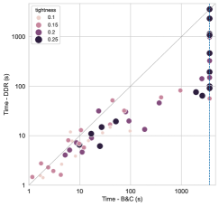
(a) Tightness

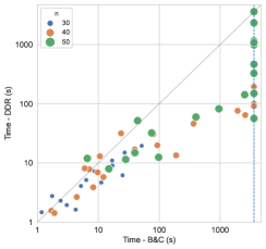
(b) Number of variables

Figure 3: (Coloured) Scatter plots comparing runtimes between B&C and DDR based on the constraint tightness and the number of variables. Dashed lines (in blue) represent the time-limit mark at 3,600 seconds. Both horizontal and vertical coordinates are in logarithmic scale.

Figure 3 depict runtimes through scatter plots that highlight instance tightness (Figure 3a) and the number of variables $n$ (Figure 3b). Dashed lines (blue) mark the time-limit coordinate at 3,600 seconds. Runtimes for DDR also include the DD construction. In total, B&C and DDR solve 47 and 59 instances out of 60, respectively. The runtime for instances solved by B&C is on average 208 seconds with a high variance (standard deviation of 592.5 seconds), while the runtime for DDR for the same instances is 18 seconds with a standard deviation of 27.5 seconds.

Figure 3a suggests that the performance is equivalent for small tightness values (0.1 and 0.15), which represent settings where only few solutions are feasible. However, as tightness increases (0.2 and 0.25), the problem becomes significantly more difficult for both solvers. In particular, while the size of DDR also increases with $t$ (since DDs would represent a larger number of solutions), the model still scales more effectively; instances with tightness of 0.20 and 0.25 are solved in 260.1 seconds on average by DDR. This is at least one order of magnitude faster than B&C, which could not solve the majority of instances with $t\geq 0.2$ within the time limit. We note that an analogous analysis follows for Figure 3b, as larger values of $n$ increase the difficulty of the problem for both methods and the same scaling benefits are observed.

Based on these results, we generate two new classes of challenging instances to assess at which point DDR would still be sufficiently compact to provide benefits with respect to B&C. To this end, the first and second class draw the knapsack coefficients uniformly at random from the discrete uniform distributions $\textnormal{U}(1,50)$ and $\textnormal{U}(1,100)$, respectively, as opposed to $\textnormal{U}(1,25)$. Larger domain distributions significantly increase the DD sizes, since the number of nodes per layers is bounded above by such numbers (we refer to Appendix 16 for the final DD sizes). We also vary the tightness within the set $\{0.1,\dots,0.9\}$ which also impacts the total number of nodes as discussed above. The number of variables is fixed to $n=30$, generating in total 45 instances for each new class with five random instances per configuration.

Figures 4a and 4b depict the aggregated results for distributions $\textnormal{U}(1,50)$ and $\textnormal{U}(1,100)$, respectively. Each plot is a performance profile that measures the number of instances solved up to each runtime. We observe that, while instances are more challenging due to larger DD sizes, DDR still solves the 45 problems within the time limit for $\textnormal{U}(1,50)$ and is significantly faster (often by orders of magnitude) than B&C. For $\textnormal{U}(1,100)$, B&C and DDR are comparable, indicating the DD size threshold at which DDRs are still beneficial for this problem class. Surprisingly, we observe that for parameters where DDR could potentially suffer from scalability issues (i.e., larger tightness and distribution domains), the resulting problem is also challenging to B&C, even with a relatively small number of variables $n$.

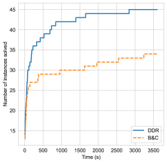
(a) U(1,50)

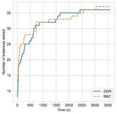
(b) U(1,100)

Figure 4: (Coloured) Performance profile plot for varying uniform discrete distribution of the knapsack constraint coefficients $a^{F}$ and $a^{L}$.

5.4 Generalizations

We end this section by discussing extensions of our approach to more general problem settings. Consider a problem setting given by

$$\max_{x^{L},x^{F}} \quad g^{L}(x^{L},x^{F})$$ (53a)

s.t. $$\quad H^{L}(x^{L},x^{F})\leq 0\;\;$$ (53b)

$$\quad x^{F}\in\argmax_{\overline{x}^{F}}\left\{g^{F}(\overline{x}^{F})\colon H^{F}(\overline{x}^{F})\leq 0,\;\;\overline{x}^{F}_{i}\leq 1-\mu_{i}(x^{L}),\;\forall i=1,\dots,n,\;\;\overline{x}^{F}\in\{0,1\}^{n}\right\}$$ (53c)

$$\quad x^{L}\in\{0,1\}^{n},$$ (53d)

where $g^{L}$, $H^{L}:\{0,1\}^{n\times n}\rightarrow\mathbb{R}$ are (possibly nonconvex) functions defined over $\{0,1\}^{n\times n}$; $g^{F}$, $H^{F}:\{0,1\}^{n}\rightarrow\mathbb{R}$ are (possibly nonconvex) functions defined over $\{0,1\}^{n}$, and $\mu_{i}:\{0,1\}^{n}\rightarrow\left\{0,1\right\}$ for all $i\in\left\{1,\dots,n\right\}$. As before, we assume the relatively complete recourse property and that all functions are well-defined over their domains.

Now consider a decision diagram $\mathcal{D}^{F}=(\mathcal{N},\mathcal{A},\nu,l)$ that exactly encodes the discrete optimization problem with feasible set:

$$\mathcal{X}=\{x\in\{0,1\}^{n}\colon H^{F}(x)\leq 0\}$$ (54)

and objective $f(x)=g^{F}(x)$, i.e., paths in $\mathcal{D}^{F}$ correspond to follower solutions that satisfy $H^{F}(x)\leq 0$ and path lengths correspond to exact evaluations of function $g^{F}$. Our reformulation procedure and all the results in propositions 5.1 – 5.8 can be directly extended for the more general setting above by defining the side constraints as

$$y_{a}\leq 1-\mu_{\tau_{a}}(x^{L}),\;\;\forall a\in\mathcal{A}\colon\nu_{a}=1,$$ (55)

because there is nothing in our methodology that requires the leader or follower problem to be linear. The main two conditions for our results to hold are that the follower problem is correctly encoded by $\mathcal{D}^{F}$ and that the effect of the leader variables on the follower problem happens exclusively via linking constraints of the form $\overline{x}^{F}_{i}\leq 1-\mu_{i}(x^{L})$.

Using our approach, we generate a single-level reformulation of (53) given by

$$\max_{x^{L},x^{F},y,\pi,\gamma} \quad g^{L}(x^{L},x^{F})$$ (MILP-DB)

s.t. $$\quad H^{L}(x^{L},x^{F})\leq 0,$$ (56a)

$$\quad\eqref{follow:ref1.1}-\eqref{follow:ref1.2},\eqref{follow:ref2}-\eqref{follow:ref2.5},\eqref{follow:ref4}-\eqref{follow:refVars},$$ (56b)

$$\quad y_{a}\leq 1-\mu_{\tau_{a}}(x^{L}),\;\;\forall a\in\mathcal{A}\colon\nu_{a}=1,$$ (56c)

$$\quad l^{\top}y-\pi_{\mathbf{r}}-\sum_{a\in\mathcal{A}\colon\nu_{a}=1}\gamma_{a}+\sum_{a\in\mathcal{A}\colon\nu_{a}=1}M_{a}\mu_{\tau_{a}}(x^{L})=0,$$ (56d)

$$\quad\gamma_{a}-M_{a}\mu_{\tau_{a}}(x^{L})\geq 0, \forall a\in\mathcal{A}\colon\nu_{a}=1,$$ (56e)

$$\quad x^{L}\in\{0,1\}^{n}.$$ (56f)

We remark that (56) is a single-level problem that conserves the original functions $g^{L}$, $H^{L}$, and $\mu_{i}$ while replacing functions $g^{F}$ and $H^{F}$ with a series of linear constraints based on the variables of a primal flow problem over $\mathcal{D}^{F}$ and the corresponding dual variables.

6 Discrete Robust Optimization

In this section, we introduce a CSP-$\mathcal{D}$ reformulation to robust problems of the form

$$\min_{x\in\mathcal{X}} \quad f(x)$$ (RO)

s.t. $$\quad A(\delta)\,x\leq b(\delta), \forall\delta\in\Delta,$$ (57)

where $\mathcal{X}$ is a discrete set as in DO, $\delta$ are realizations of a (possibly infinite) uncertainty set $\Delta$, and $A(\delta)\in\mathbb{R}^{r\times n}$, $b(\delta)\in\mathbb{R}^{r}$ are the coefficient matrix and the right-hand side, respectively, for the realization $\delta\in\Delta$ for some $r>0$. As discussed in §2, state-of-the-art algorithms for DO first relax the model by considering only a subset of $\Delta$ in (57), iteratively adding violated constraints from missing realizations until convergence.

We propose an alternative algorithm for RO that is applicable when the set $\mathcal{X}$ is amenable to a DD encoding. The potential benefit of the methodology is that it is combinatorial and exploits the network structure of $\mathcal{D}$ for scalability purposes. Our required assumptions are the existence of a separation oracle $\mathscr{S}(x)$ that identifies violations of (57), i.e.,

$$\mathscr{S}(x)=\left\{\begin{array}[]{ll}(i,\delta),&\textnormal{for any $(i,\delta)\in\{1,\dots,r\}\times\Delta$ such that $a_{i}(\delta)x>b_{i}(\delta)$},\\ \emptyset,&\textnormal{if no such pair exists,}\end{array}\right.$$ (60)

and that such oracle returns either a pair $(i,\delta)$ or $\emptyset$ in finite computational time. This is a mild assumption in existing RO formulations and holds in typical uncertainty sets, such as when $\Delta$ is an interval domain or, more generally, has a polyhedral description. For instance, if $\Delta$ is finite (e.g., derived from a sampling process), then the simplest $\mathscr{S}(x)$ enumerates each $\delta$ separately.

We start in §6.1 with a reformulation of the robust problem as a CSP-$\mathcal{D}$, leveraging this time the dynamic programming perspective presented in §4.3. Next, we discuss a state-augmenting procedure to address the resulting model in §6.2, and perform a numerical study on a robust variant of the traveling salesperson problem with time windows (TSPTW) in §6.3.

6.1 Reformulation of RO

Let $\mathcal{D}^{R}=(\mathcal{N},\mathcal{A},\nu,l)$ encode the discrete optimization problem DO with feasible set $\mathcal{X}$ and objective $f(x)$. The constrained longest-path reformulation is obtained directly by representing (57) as side constraints over the arc space of $\mathcal{D}^{R}$, which we formalize in Proposition 6.1.

Proposition 6.1

For each arc $a$ of $\mathcal{D}^{R}$, $\delta\in\Delta$, and $i\in\{1,\dots,r\}$, define the scalars

$$g_{i,a}(\delta)=\nu_{a}\,a_{i,\tau_{a}}(\delta),$$ (61)

where $a_{i,\tau_{a}}(\delta)$ is the $(i,\tau_{a})$-th element of $A(\delta)$. Let $G(\delta)=\{g_{i,a}(\delta)\}_{\forall i,a}$ be the matrix composed of such scalars for each $\delta$. There exists a one-to-one mapping between solutions $x$ of RO and paths of CSP-$\mathcal{D}$ defined over $\mathcal{D}^{R}$ and with side constraints

$$G(\delta)\,y\leq b(\delta), \forall\delta\in\Delta.$$ (62)

Modeling such a reformulation as MILP-$\mathcal{D}$ often results in a binary mathematical program with exponential or potentially infinite many constraints. However, it may be tractable in the presence of special structure. If inequalities (62) preserve the totally unimodularity of the network matrix in (3)-(4), and are separable in polynomial time, then MILP-$\mathcal{D}$ is solvable in polynomial time in $\mathcal{D}^{R}$ via the Ellipsoid method (Grötschel et al. 2012). Otherwise, computational approaches often rely on decomposition methods that iteratively add variables and constraints to the MILP.

6.2 State-augmenting Algorithm

We propose a state-augmenting approach where each iteration is a traditional combinatorial constrained shortest-path problem and is amenable, e.g., to combinatorial methods such as the pulse method (Cabrera et al. 2020). Our solution is based on recursive model DP-$\mathcal{D}$ as applied to RO. More precisely, we solve the recursion

$$V_{u}(\dot{}s)=\left\{\begin{array}[]{ll}\min_{a\in\Gamma^{+}({u})\colon s+G_{a}\leq d}\left\{l_{a}+V_{h_{a}}(\dot{}s+G_{a})\right\},&\textnormal{if $u\neq\mathbf{t}$,}\\ 0,&\textnormal{otherwise.}\end{array}\right.$$ (65)

with state space defined by the elements $\dot{}s=(\;s(\delta)\;)_{\forall\delta\in\Delta},$ where each $s(\delta)\in\mathbb{R}^{r}$ is the state vector encoding the $\delta$-th inequalities $G(\delta)\,y\leq b(\delta)$ of (62).

We recall that, if solved via the shortest-path representation LP-$\mathcal{D}$, an optimal solution corresponds to a sequence $(\dot{}s_{1},a_{1}),\dots(\dot{}s_{n},a_{n})$ where $(a_{1},\dots,a_{n})$ is an $\mathbf{r}-\mathbf{t}$ path in $\mathcal{D}^{R}$ and $\dot{}s_{i}\in\mathcal{S}_{t_{a_{i}}}$ is a reachable state at node $t_{a_{i}}$, $i\in\{1,\dots,n\}$. We formalize two properties of the DP model based on this property, which build on the intuition that states conceptually play the role of constraints in recursive models. In particular, we show that only a finite set of realizations are required in the state representation to solve the Bellman equations exactly, providing a “network counterpart” of similar results in infinite-dimensional linear programs.

Proposition 6.2

Let $z(\Delta^{\prime})$ be an optimal solution of DP-$\mathcal{D}$ when the state vector $\dot{}s$ is written only with respect to a subset of realizations $\Delta^{\prime}\subseteq\Delta$, adjusting the dimension of $d$ appropriately. Then,

1. $z(\Delta^{\prime})\leq z(\Delta^{\prime\prime})$ for any $\Delta^{\prime}\subseteq\Delta^{\prime\prime}\subseteq\Delta$.

2. There exists a finite subset $\Delta^{*}\subseteq\Delta$ such that $z(\Delta^{*})=z(\Delta)$.

Proof 6.3

Proof of Proposition 6.2. Property (a) follows because DP-$\mathcal{D}$ is equivalent to RO for any $\Delta^{\prime}\subseteq\Delta$ due to Proposition 6.1 (correctness of the reformulation) and Proposition 4.2 (correctness of DP-$\mathcal{D}$). Thus, since RO written in terms of $\Delta^{\prime}$ has less constraints than the same model written in terms of $\Delta^{\prime\prime}$, we must have $z(\Delta^{\prime})\leq z(\Delta^{\prime\prime})$.

For property (b), let $\mathcal{P}$ be the finite set of $\mathbf{r}-\mathbf{t}$ paths in $\mathcal{D}^{R}$. Partition $\mathcal{P}$ into subsets $\mathcal{P}^{F}$ and $\mathcal{P}^{I}=\mathcal{P}\setminus\mathcal{P}^{F}$, where $p\in\mathcal{P}^{F}$ if and only if its associated solution $x^{p}$ is feasible to RO. Thus, for each $\hat{p}\in\mathcal{P}^{I}$, there exists at least one scenario $\delta^{\hat{p}}\in\Delta$ where some inequality of $A(\delta^{\hat{p}})\leq b(\delta^{\hat{p}})$ is violated. We build the set

$$\Delta^{*}=\bigcup_{\hat{p}\in\mathcal{P}^{I}}\{\delta^{\hat{p}}\}$$

which is also finite and must be such that $z(\Delta^{*})=z(\Delta)$, since only paths in $\mathcal{P}^{F}$ are feasible to CSP-$\mathcal{D}$ which, by definition, are also feasible to RO. $\blacksquare$

Proposition 6.2 and its proof suggest a separation algorithm that identifies a sequence of uncertainty sets $\Delta_{1}\subset\Delta_{2}\subset\dots\subset\Delta_{k}=\Delta^{*}$ providing lower bounds to RO in each iteration, identifying scenarios to compose $\Delta^{*}$. We describe it in Algorithm 1, which resembles a Benders decomposition applied to a recursive model, i.e., the state variables of LP-$\mathcal{D}$ encode the Benders cuts and the master problem is solved in a combinatorial way $\mathcal{D}$ via a constrained shortest-path algorithm.

The algorithm starts with $\Delta_{1}=\emptyset$ and finds an optimal $\mathbf{r}-\mathbf{t}$ path on $\mathcal{D}^{R}$. Notice that such path can be obtained by any shortest-path algorithm because the state space is initially empty. Next, the separation oracle $\mathscr{S}(x^{*})$ is invoked to verify if there exists a realization $\delta$ for which inequalities (57) are violated. If that is the case, the state vector $\dot{}s$ is augmented and the problem is resolved with a constrained shortest path algorithm. Otherwise, the algorithm terminates.

1:Let $\Delta_{1}=\emptyset$, $t=1$.

2:Let $x^{*}=(x_{\nu_{a_{1}}},\dots,x_{\nu_{a_{n}}})$ be derived from an optimal $\mathbf{r}-\mathbf{t}$ path $(a_{1},\dots,a_{n})$ in LP-$\mathcal{D}$ w.r.t. $\Delta_{1}$.

3:while there exists $(i,\delta)=\mathscr{S}(x^{*})\neq\emptyset$ do

4:     $\Delta_{t+1}=\Delta_{t}\cup\{\delta\}$.

5:     Resolve LP-$\mathcal{D}$ using the augmented state vector $\dot{}s$ w.r.t. $\Delta_{t+1}$.

6:     Set $x^{*}=(x_{\nu_{a_{1}}},\dots,x_{\nu_{a_{n}}})$ from the optimal $\mathbf{r}-\mathbf{t}$ path $(a_{1},\dots,a_{n})$.

7:     $t:=t+1$.

8:return $x^{*}$.

Algorithm 1 State-augmenting Algorithm (Input: RO, Output: Optimal $x^{*}$)

In each iteration of the algorithm, $f(x^{*})$ provides a lower bound on the optimal value of RO according to Proposition 6.2. Once $\mathscr{S}(x^{*})=\emptyset$, we obtain a feasible solution $x^{*}$ to RO and, thus, an optimal solution to the problem.

We provide a formal proof of the convergence of the algorithm below. Specifically, the worst-case complexity of the state-augmenting algorithm is a function of both (i) the number of paths in $\mathcal{D}^{R}$, (ii) the worst-case time complexity of the separation oracle $\mathscr{S}(x)$, and (iii) the worst-case complexity of the solution approach to LP-$\mathcal{D}$ to be applied. We observe that, computationally, the choice of each $\delta$ to include plays a key role in numerical performance, which we discuss in our case study of §6.3.

Proposition 6.4

Algorithm 1 terminates in a finite number of iterations. Moreover, the number of calls to the separation oracle $\mathscr{S}(\cdot)$ is bounded above by the number of infeasible paths of $\mathcal{D}^{R}$ with respect to (62).

6.3 Case Study: Robust Traveling Salesperson Problem with Time Windows

We investigate the separation algorithm on a last-mile delivery problem with uncertain service times and model it as a robust traveling salesperson problem with time windows (RTSPTW). Let $G=(\mathcal{V},\mathcal{E})$ be a directed graph with vertex set $\mathcal{V}=\{0,1,\dots,n\}$ and edge set $\mathcal{E}\subseteq\mathcal{V}\times\mathcal{V}$, where $0$ and $n$ are depot vertices. With each vertex $j\in\mathcal{V}\setminus\{0\}$ we associate a time window $[r_{j},d_{j}]$ for a release time $r_{i}$ and a deadline $d_{j}$, and with each edge $(i,j)$ we associate non-negative cost $c_{ij}$ and travel time $t_{ij}$. Moreover, visiting a vertex $j\in\mathcal{V}\setminus\{0\}$ incurs a random service time $\delta_{j}$. The uncertainty values $\delta=(\delta_{1},\dots,\delta_{n})$ are described according to a non-empty budgeted uncertainty set

$$\Delta=\left\{\delta\in\mathbb{Z}^{n}\colon\sum_{j\in\mathcal{N}}\delta_{j}\leq b,\;\;l_{j}\leq\delta_{j}\leq u_{j}\;\;\forall j\in\mathcal{N}\right\},$$

where $l_{j},u_{j}\geq 0$ are lower and upper bounds on the service time of vertex $j$, respectively, and $b$ is an uncertainty budget that controls how risk-averse the decision maker is (Bertsimas and Sim 2004). More precisely, lower values of $b$ indicate that scenarios for which all vertices of $\mathcal{V}$ will have high service times are unlikely and do not need to be hedged against. Converserly, larger values of $b$ imply that the decision maker is more conversative in terms of the worst case; in particular, $b\rightarrow+\infty$ represents a classical interval uncertainty set.

The objective of the RTSPTW is to find a minimum-cost route (i.e., a Hamiltonian path) starting at vertex $0$ and ending at vertex $n$ that observes time-window constraints with respect to the edge travel times. We formalize it as the MILP

$$\min_{x,\mathbf{w}} \quad\sum_{(i,j)\in\mathcal{E}}c_{ij}x_{ij}$$ (MILP-TSP)

s.t. $$\quad\sum_{j:(i,j)\in\mathcal{E}}{x_{ij}}=1, \forall i\in\mathcal{V}\setminus\{n\},$$ (66)

$$\quad\sum_{j:(j,i)\in\mathcal{E}}{x_{ji}}=1, \forall i\in\mathcal{V}\setminus\{0\},$$ (67)

$$\quad w_{j}^{\delta}\geq w_{i}^{\delta}+(\delta_{i}+t_{ij})x_{ij}-M(1-x_{ij}), \forall(i,j)\in\mathcal{E},\delta\in\Delta,$$ (68)

$$\quad r_{j}\leq w_{j}^{\delta}\leq d_{j}, \forall j\in\mathcal{V},\boldsymbol{\delta}\in\mathcal{U},$$ (69)

$$\quad x_{ij}\in\{0,1\}, \forall(i,j)\in\mathcal{E}.$$ (70)

In the formulation above, the binary variable $x_{ij}$ denotes if the path includes edge $(i,j)\in\mathcal{E}$ and $M=d_{n}$ is a valid upper bound on the end time of any service. The variable $w^{\delta}_{j}$ is the time that vertex $j\in\mathcal{V}$ is reached when the realization of the service times is $\delta\in\Delta$. Inequalities (66)-(67) ensure that each vertex is visited once. Inequalities (68)-(69) represent the robust constraint and impose that time windows are observed in each realization $\delta\in\Delta$. Note that, since $\Delta\neq\emptyset$, they also rule out cycles in a feasible solution.

The main challenge in MILP-TSP is the requirement that routes must remain feasible for all realizations of the uncertainty set. In particular, solving MILP-TSP directly is not viable because of the exponential number of variables and constraints. Thus, existing routing solutions are not trivially applicable to this model, as analogously observed in related robust variants of the traveling salesperson problem (e.g., Montemanni et al. 2007, Bartolini et al. 2021).

6.3.1 Constrained Shortest-path Formulation.

We formulate a multivalued decision diagram $\mathcal{D}$ that encodes the Hamiltonian paths in $G$ starting at $0$ and ending at $n$. Each $\mathbf{r}-\mathbf{t}$ path $(a_{1},\dots,a_{n})$ represents the route $(0,\nu_{a_{1}},\dots,\nu_{a_{n}})$ with $\nu_{a_{n}}=n$ and $\nu_{a_{j}}\in\{1,\dots,n-1\}$ for $j\neq n$. Moreover, for simplicity of exposition, we consider that $\mathcal{D}$ represents directly a traditional DP formulation of the traveling salesperson problem (TSP), i.e., with each node $u\in\mathcal{N}$ we associate the state $(\mathcal{S}_{u},L_{u})$ where $\mathcal{S}_{u}$ contains the set of visited vertices on the paths ending at $u$, and $L_{u}\in\mathcal{V}$ gives the last vertex visited in all such paths. In particular, $(\mathcal{S}_{u},L_{\mathbf{r}})=(\{0\},0)$ and $L_{\mathbf{t}}=(\mathcal{V},n)$. We refer to Example 6.5 for an instance with five vertices and to Cire and Van Hoeve (2013) for additional details and compression techniques for $\mathcal{D}$.

Example 6.5

Figure 5 depicts $\mathcal{D}$ for a TSP with vertex set $\mathcal{V}=\{0,\dots,4\}$ where every path must start at $0$ and end at $4$. The labels on each arc denote $\nu_{a}$. For example, in the left-most node of the third layer, the state $(\mathcal{S}_{u},L_{u})=(\{0,1,2\},2)$ indicates that vertices in $\{0,1,2\}$ were visited in all paths ending at that node, and that the last vertex in such paths is $2$. Notice that the only outgoing arc $a$ has value $\nu_{a}=3$, since (i) this is the only vertex not yet visited in such path, and (ii) paths cannot finish at vertex $4$. $\square$

Figure 5: A decision diagram for a TSP problem with $n=4$ cities for Example 6.5.

The side constraints are an arc-based representation of (68). While it is possible to write an inequality system (2) in terms of arc variables $y$ by incorporating auxiliary variables, we leverage the DP perspective to obtain a more compact state representation. Specifically, for each scenario $\delta\in\Delta$ and node $u\in\mathcal{N}$, let $e_{u}(\delta)$ be the earliest time any route finishes serving vertex $L_{u}$ when considering only $\mathbf{r}-\mathbf{t}$ paths that include $u$. Formally,

$$e_{\mathbf{r}}(\delta)=0,$$ (71)

$$e_{v}(\delta)=\max\left(r_{L_{v}},\min_{(u,v)\in\Gamma^{-}({v})}e_{u}(\delta)+t_{L_{u}L_{v}}\right)+\delta_{L_{v}}, \forall v\in\mathcal{N}\setminus\{\mathbf{r}\}.$$ (72)

The first equality states that the earliest time we finish serving vertex $0$ is zero by definition. In the second equality, the “max” term corresponds to the earliest time to arrive at vertex $L_{v}$ for a node $v$, which considers its release time and all potential preceding travel time from a predecessor vertex $L_{u}$. It follows that an $\mathbf{r}-\mathbf{t}$ path is feasible if and only if

$$e_{u}(\delta)\leq d_{L_{u}}, \forall u\in\mathcal{N},\delta\in\Delta$$ (73)

and the vector $(\,\mathbf{e}(\delta)\,)_{\delta\in\Delta}$ are the node states augmented by Algorithm 1 per realization $\delta$.

Finally, we require a separation oracle $\mathscr{S}(x)$ to identify a realization violated by $x$. We propose to pick the “most violated” scenario in terms of the number of nodes for which the deadline is not observed (see Appendix 15).

6.3.2 Numerical Study.

We compare two methodologies for the RTSPTW to evaluate the benefits of the combinatorial perspective provided by DDs. The first is akin to classical approaches to RO and consists of applying Algorithm 1 using MILP-TSP when deriving a new candidate solution (Step 5); we denote such a procedure by IP. The second approach is Algorithm 1 reformulated via decision diagrams, as developed in this section. We use a simple implementation of the pulse algorithm to solve each iteration of the constraint shortest-path problems over $\mathcal{D}$ (see description in Appendix 14). We denote our approach by DD-RO. As before, we focus on graphical description of the results, with all associated tables and detail included in Appendix 16. The MILP models were solved in ILOG CPLEX 20.1. Source code is available upon request. Finally, we remark that both IP and DD-RO can be enhanced using other specialized TSPTW and constrained shortest-path formulations; here we focus on their basis comparison with respect to Algorithm 1.

Our testbed consists of modified instances for the TSPTW taken from Dumas et al. (1995). In particular, we consider classical problem sizes of $n\in\left\{40,60\right\}$ and time windows widths of $w\in\left\{20,40,60,80\right\}$, where a lower value of $w$ indicates tighter time windows and therefore less routing options. For each instance configuration, we incorporate an uncertainty set budget of $\Delta\in\left\{4,6,8,10\right\}$ and set the bounds for the service times as $l=0$ and $u=2$. To preserve feasibility we extend the upper time limit for all the nodes by $\Delta$ time units. We generate five random instance per configuration $(n,t,\Delta)$, thus 160 instances in total.

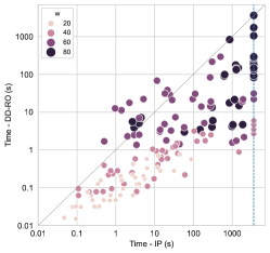
(a) Time window width $w$

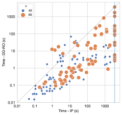
(b) Number of variables

Figure 6: (Coloured) Scatter plots comparing runtimes between IP and DD-RO based on the time-window width $w$ and the number of variables. Dashed lines (in blue) represent the time-limit mark at 3,600 seconds.

Figure 6 depict runtimes through scatter plots that compare the time-window width (Figure 6a) and the number of variables $n$ (Figure 6b), similarly to the bilevel numerical study in §5.3.2. Dashed lines (blue) mark the time-limit coordinate at 3,600 seconds. In total, IP and DD-RO solve 137 and 159 instances out of 160, respectively. The runtime for the instances solved by IP is on average 241.9 with a standard deviation of 541.3 seconds, while the runtime for DD-RO for the same instances is 22.1 seconds with a standard deviation of 82.1 seconds.

Figure 6a suggests that the complexity of instances is highly affected by time-window width for both methods. In particular, small values of $w$ lead to smaller decision diagrams, and hence faster pulse runtimes. We observe an analogous pattern in Figure 6b, where larger values of $n$ reflect more difficult instances. On average, runtimes for DD-RO were at least 75 times faster than IP, which underestimates the real value since many instances were not solved to optimality by IP. The reason follows from the time per iteration between using pulse and MILP in Algorithm 1. While both theoretically have the same number of iterations in such instance, pulse is a purely combinatorial approach over $\mathcal{D}$ and solves the constrained shortest-path problem, on average, in 40 seconds per iteration. For IP, the corresponding model MILP-TSP (with fewer scenarios) is challenging to solve, requiring 234 seconds per iteration on average.

7 Conclusion

We study reformulations of discrete bilevel optimization problems and robust optimization as constrained shortest-path problems (CSP). The methodology consists of reformulating portions of the original problem as a network model, here represented by decision diagrams. The remaining variables and constraints are then incorporated as parameters in budgeted resources over the arcs of the network, reducing the original problem to a CSP.

We propose two approaches to solve the underlying CSP based on each setting. For the bilevel case, we leverage polyhedral structure to rewrite the original problem as a mixed-integer linear programming model, where we convexify non-linear terms connecting the master’s and follower’s variables by exploiting duality over the network structure. For the robust case, we proposed a state-augmenting algorithm that iteratively add labels (i.e., resources) to existing dynamic programming approaches to CSPs, which only rely on the existence of a separation oracle that identifies violated realizations of a solution.

The methods were tested on a competitive project selection problem, where the follower and the leader must satisfy knapsack constraints, and on a robust variant of a traveling salesperson problem with time windows. In both settings, numerical results suggested noticeable improvements in solution time of the CSP-based techniques with respect to state-of-the-art methods on the tested instances, often by orders of magnitude.

Dr. Lozano gratefully acknowledges the support of the Office of Naval Research under grant N00014-19-1-2329, and the Air Force Office of Scientific Research under grant FA9550-22-1-0236.

8 Proof of Proposition 4.1

We reduce the knapsack problem to a formulation of CSP-$\mathcal{D}$ with the required size. Consider any knapsack instance

$$\max_{x}\left\{px\colon cx\leq b,\;\;x\in\{0,1\}^{n}\right\}$$

for $a,c\in\mathbb{R}^{N}$ and $b\in\mathbb{R}^{*}_{+}$. Consider now a one-width decision diagram having all $n$ permutations of $\{0,1\}$, that is, $\mathcal{D}$ has one node per layer and every node except $\mathbf{t}$ has two ougoing arcs, one per each value assignment $\nu_{a}\in\{0,1\}$. For example, the figure below depicts $\mathcal{D}$ for $n=4$:

Since $\mathcal{D}$ encodes the binary set $\{0,1\}^{n}$, it suffices to define side inequalities (2) that replicate the knapsack constraint, i.e., we fix $m=1$, coefficients $G_{1a}=c_{\tau_{a}}\nu_{a}$ for all $a\in\mathcal{A}$, and $d=b$. Finally, for the objective, we have the lengths $l_{a}=-p_{\tau_{a}}\nu_{a}$ for all $a\in\mathcal{A}$, assumed negative since CSP-$\mathcal{D}$ is a “min” problem (or, equivalently, we could also change the objective sense to “max”). Thus, there is a one-to-one correspondance between a knapsack instance and a solution to CSP-$\mathcal{D}$, and their optimal solution values match. $\blacksquare$

9 Proof of Proposition 5.1

Consider the $\mathbf{r}-\mathbf{t}$ arc-specified path $p=(a_{1},a_{2},\dots,a_{n})$ in $\mathcal{D}^{F}$ extracted from an arbitrary feasible solution $y$ of CSP-$\mathcal{D}$. The associated solution vector $x^{p}=(\nu_{a_{1}},\nu_{a_{2}},\dots,\nu_{a_{n}})$ satisfies $A^{F}x^{p}\leq b^{F}$ by construction of $\mathcal{D}^{F}$. Further, because of (18), we can only have $x^{p}_{j}=\nu_{a_{j}}=1$ for some $j\in\{1,\dots,n\}$ if $x^{L}_{j}=0$, that is, $x^{p}\leq\mathbf{1}-x^{L}$. Thus, since the solution values and path lengths match by construction of $\mathcal{D}^{F}$, an optimal solution of the corresponding CSP-$\mathcal{D}$ satisfies (15), and the converse holds analogously. $\blacksquare$

10 Proof of Proposition 5.8

From Proposition 5.4 we have that valid $M$-values should be large enough to provide an upper bound for the $\gamma$-variables. Consider any feasible solution to MILP-DB given by $({\hat{x}^{L},\hat{x}^{F},\hat{y},\hat{\pi},\hat{\gamma}})$ and note that for all arcs $a\in\mathcal{A}$ such that $\hat{x}^{L}_{\tau_{a}}=1$ and $\nu_{a}=1$, the corresponding dual $\gamma$-variables could take any value in the range

$$\hat{\gamma}_{a}\in[l_{a}+\hat{\pi}_{h_{a}}-\hat{\pi}_{t_{a}},\infty],$$

preserving feasibility. Assume without loss of generality that

$$\hat{\gamma}_{a}=l_{a}+\hat{\pi}_{h_{a}}-\hat{\pi}_{t_{a}},\quad\forall a\in\mathcal{A}\colon x^{L}_{\tau_{a}}=1\text{ and }\nu_{a}=1,$$ (74)

that is, $\hat{\gamma}_{a}$ is the shadow price corresponding to constraints (33) and captures the change in the objective function associated with adding one unit of capacity to arc $a$. The values for $\hat{\pi}_{h_{a}}$ and $\hat{\pi}_{t_{a}}$ are computed as the length of the best completion path from nodes $h_{a}$ and $t_{a}$ to $\mathbf{t}$, if a completion path exists, or some arbitrary value otherwise. The relatively complete recourse property ensures that there exists at least one path from $\mathbf{r}$ to $\mathbf{t}$ and as a result

$$\sum_{j=1}^{n}\min\{c_{j}^{F},0\}\leq\hat{\pi}_{i}\leq\sum_{j=1}^{n}\max\{c_{j}^{F},0\},\quad\forall i\in\mathcal{N}.$$ (75)

Combining (74) and (75) we obtain that

$$\hat{\gamma}_{a}\leq l_{a}+\sum_{j=1}^{n}\max\{c_{j}^{F},0\}-\sum_{j=1}^{n}\min\{c_{j}^{F},0\},\quad\forall a\in\mathcal{A}\colon x^{L}_{\tau_{a}}=1\text{ and }\nu_{a}=1,$$ (76)

completing the proof. $\blacksquare$

11 Proof of Proposition 6.1

By construction of $\mathcal{D}^{R}$, there is a one-to-one correspondence between paths of $\mathcal{D}^{R}$ and solutions of $\mathcal{X}$. Consider the $\mathbf{r}-\mathbf{t}$ arc-specified path $p=(a_{1},a_{2},\dots,a_{n})$ in $\mathcal{D}^{R}$ extracted from an arbitrary feasible solution $y$ of CSP-$\mathcal{D}$, and let $x^{p}=(\nu_{a_{1}},\nu_{a_{2}},\dots,\nu_{a_{n}})\in\mathcal{X}$ be its associated solution. Then, for any $\delta\in\Delta$ and $i\in\{1,\dots,r\}$,

$$b_{i}(\delta)\geq g_{i}(\delta)\,y=\sum_{a\in\mathcal{A}}g_{i,a}(\delta)\,y_{a}=\sum_{a\in\mathcal{A}}\nu_{a}\,a_{i,\tau_{a}}(\delta)\,y_{a}=\sum_{j=1}^{n}a_{i,j}(\delta)\nu_{a_{j}}=\sum_{j=1}^{n}a_{i,j}(\delta)x^{p}_{j}=a_{i}x^{p}.$$

That is, $x^{p}$ is feasible to RO. Conversely, any feasible solution to RO can be shown feasible to CSP-$\mathcal{D}$ by applying the same steps, noticing that the objective functions are equivalent. $\blacksquare$

12 Proof of Proposition 6.4

At any iteration $t$, the algorithm either (i) stops, in which case the solution is optimal since $\Delta_{t+1}\subset\Delta$; or (ii) $x^{*}$ is infeasible due to some scenario $\delta$. Because $\delta$ belongs to the future sets $\Delta_{t+2},\Delta_{t+3},\dots$, we must have that $x^{*}$ is infeasible to LP-$\mathcal{D}$ at any future iterations, i.e., its associated path is never selected as an optimal $\mathbf{r}-\mathbf{t}$ path. Thus, since the number of paths of $\mathcal{D}^{R}$ is finite, the algorithm must terminate after all infeasible paths have been exhausted. $\blacksquare$

13 Decision Diagram Modeling

In this section, we briefly discuss the two general steps of modeling a problem as a discrete optimization problem DO; additional details and examples are provided in Bergman et al. (2016). Specifically, the first step rewrites the problem as the recursive model

$$\min_{x,s} \quad\sum_{i=1}^{n}\hat{f}(s_{i},x_{i})$$

s.t. $$\quad s_{i+1}=T_{i}(s_{i},x_{i}), \forall i\in\{1,\dots,n\},$$

$$\quad x_{i}\in\mathcal{X}(s_{i}), \forall i\in\{1,\dots,n\},$$

where $s_{1},\dots,s_{n},s_{n+1}$ are state variables, $T_{i}(s_{i},x_{i})$ for all $i=1,\dots,n$ are state-transition functions, $\hat{f}(s_{i},x_{i})$ are cost functions, and $\mathcal{X}(s_{i})$ are the possible values that variable $x_{i}$ admits given the state element $s_{i}$. A recursive reformulation is valid when the feasible vectors $x$ of the system above have a one-to-one relationship with $\mathcal{X}$ and $\sum_{i=1}^{n}\hat{f}(s_{i},x_{i})=f(x)$. For instance, for the knapsack problem

$$\max_{x} \quad\sum_{j=1}^{n}c_{j}x_{j}$$

s.t. $$\quad\sum_{j=1}^{n}a_{j}x_{j}\leq b$$

$$\quad x_{j}\in\{0,1\}, \forall j\in\{1,\dots,n\},$$

with $a$ and $c$ non-negative, the recursive model is

$$\max_{x,s} \quad\sum_{j=1}^{n}c_{j}x_{j}$$

s.t. $$\quad s_{j+1}=s_{j}+a_{j}x_{j}, \forall j\in\{1,\dots,n\}$$

$$\quad s_{j}+a_{j}x_{j}\leq b, \forall j\in\{1,\dots,n\},$$

$$\quad x_{j}\in\{0,1\}, \forall j\in\{1,\dots,n\},$$

$$\quad s_{1}=0$$

that is, $s_{j}$ encodes the knapsack load at the $j$-th stage, $T_{i}(s_{j},x_{j})=s_{j}+a_{j}x_{j}$, $\hat{f}(s_{j},x_{j})=c_{j}x_{j}$, and $\mathcal{X}(s_{j})=\{x\in\{0,1\}\colon s_{j}+a_{j}x_{j}\leq b\}$.

Given the recursive formulation above, we write the initial $\mathcal{D}$ as the underlying state-transition graph, i.e., the $j$-th layer $\mathcal{N}_{j}$ includes one node per possible value of $s_{j}$, and there exists an arc with label $x_{j}$ between two nodes $s_{j}$, $s_{j+1}$ if and only if $s_{j+1}=s_{j}+a_{j}x_{j}$ and $x_{j}\in\mathcal{X}(s_{j})$. The length of such an arc is set to $\hat{f}(s_{i},x_{i})$. For example, consider the knapsack instance from Example 3.1:

$$\max_{x}\quad 4x_{1}+3x_{2}+7x_{3}+8x_{4}$$

s.t. $$7x_{1}+5x_{2}+4x_{3}+x_{4}\leq 8,$$

$$x_{1},x_{2},x_{3},x_{4}\in\{0,1\}.$$

The resulting (non-reduced) $\mathcal{D}$ is as follows, where node labels correspond to the states $s_{j}$ and arc labels to $\hat{f}(s_{i},x_{i})$. We also represent all possible values of $s_{n+1}$ into a single terminal node $\mathbf{t}$ with no loss of information. For exposition purposes, we also omit the labels on the last arcs, which are all equivalent ($0$ for dashed arcs, and $1$ for solid arcs).

    

Finally, the second step of the procedure is known as reduction, where we compress the graph by eliminating redundant nodes. For example, all nodes in the fourth layer can be compressed into a single node, since they have equivalent paths to $\mathbf{t}$. More precisely, two nodes $u,u^{\prime}\in\mathcal{N}_{j}$ are redundant if their outgoing arcs are equivalent, that is, for each arc $a$ outgoing from $u$, there exists another arc $a^{\prime}$ with the same head node, length, and value; and vice-versa for node $u^{\prime}$. The reduction procedure is a bottom-up traversal that merges nodes if their outgoing arcs are equivalent, i.e.,

1. For each layer $j=n,n-1,n-2,\dots,2$:

   1. If there are two redundant nodes $u,u^{\prime}\in\mathcal{N}_{j}$, then merge them into a single node, redirecting the corresponding incoming arcs.

Figure 1(a) depictes the resulting graph after applying the reduction mechanism above.

14 The Pulse Algorithm

The pulse algorithm proposed originally by Lozano and Medaglia (2013), is a recursive enumerative search based on the idea of propagating a pulse through a directed network, starting at the root node. Pulses represent partial paths and propagate through the outgoing arcs from each node, storing information about the partial path being explored. Once a pulse corresponding to a feasible path reaches the end node, the algorithm updates a primal bound on the objective function, stops the pulse propagation, and backtracks to continue the recursive search resulting in a pure depth-first exploration. Opposite to labelling algorithms, pulses are not stored in memory but passed as arguments in the recursive search function. If nothing prevents pulses from propagating, the pulse algorithm enumerates all feasible paths from root node to end node ensuring that an optimal path is found.

To avoid a complete enumeration of the solution space, the pulse algorithm employs a set of pruning strategies proposed to prune pulses corresponding to partial paths, without cutting off an optimal solution. The core strategies in the pulse algorithm are pruning by infeasibility, bounds, and dominance. The infeasibility pruning strategy uses a dual bound on the minimum resource required to reach the end node from any given intermediate node and discards partial paths that cannot be completed into a feasible complete path. The bounds pruning strategy uses dual bounds on the minimum-cost (maximum-profit) paths from any intermediate node to the end node and discards partial paths that cannot be part of an optimal solution. The dominance pruning strategy uses a limited number of labels to store information on partial paths explored during the search and discard partial paths based on traditional dominance relationships. In contrast to labeling algorithms, the pulse algorithm does not rely on extending every non-dominated label for correctness; instead, this is guaranteed by properly truncating the recursive search. Hence, even if no labels were used at any of the nodes, the algorithm remains correct.

The pulse algorithm has been extended for the elementary shortest path problem with resource constraints (Lozano et al. 2015), the biobjective shortest path problem (Duque et al. 2015), the weight constrained shortest path problem with replenishment (Bolívar et al. 2014), the orienteering problem with time windows (Duque et al. 2014), and more recently, the robust shortest path problem (Duque and Medaglia 2019). Beyond the domain of shortest path problems, several authors have used the pulse algorithm as a component to solve other hard combinatorial problems. For instance, the pulse algorithm has been used in network interdiction (Lozano and Smith 2017b), shift scheduling (Restrepo et al. 2012), evasive flow (Arslan et al. 2018), resource constrained pickup-and-delivery (Schrotenboer et al. 2019), and green vehicle routing problems (Montoya et al. 2016), among others.

15 Separating the Most Violated Scenario for RTSPTW

For ease of notation, let $r_{0}=0$ and $d_{0}=+\infty$. To separate the scenario in which the deadlines are most violated we solve model SEP-TSP for a fixed $x$:

$$\max_{\mathbf{v},\delta,\mathbf{w}} \quad\sum_{j\in\mathcal{V}}v_{j}$$ (SEP-TSP)

s.t. $$\quad w_{0}=0,$$ (77)

$$\quad w_{j}=\max\{r_{j},w_{i}+\delta_{i}+t_{ij}\}, \forall(i,j)\in\mathcal{E}\colon x_{ij}=1,$$ (78)

$$\quad w_{j}\geq(d_{j}+\epsilon)v_{j}, \forall j\in\mathcal{V},$$ (79)

$$\quad\delta\in\Delta,v_{j}\in\{0,1\}, \forall j\in\mathcal{V}.$$ (80)

In our separation model, $v_{j}=1$ if and only if the time window of vertex $j$ is violated, $j\in\mathcal{V}$. The equalities (77)-(78) specify the arrival times $\mathbf{w}$ that follow from $x$. The inequalities (79) enforce the definition of $v_{j}$ considering a sufficiently small $\epsilon$ (e.g., the machine precision). Finally, (80) specify the domain of variables. We note that SEP-TSP can be solved by MILP solvers after linearizing the “max” in (78) with additional binary variables.

16 Additional Tables

16.1 Competitive Project Scheduling

Table 1 presents extended results for our experiments with competitive scheduling instances. The first column indicates the number of items. The second column presents the budget tightness parameter. Columns 3 to 8 present for each algorithm the average computational time in seconds calculated among the 5 instances of the same configuration, the number of instances solved within the time limit, and the average optimality gap computed over the instances not solved within the time limit. We use a dash in the “Gap” column to indicate that all instances in the row are solved to optimality. For instances not solved within the time limit we record a computational time of $3600$ seconds. Columns 9 and 10 present for the DD-based approach the average number of nodes and arcs in the resulting DD.

Table 1: Comparing B&C and DDR on a set of synthetic competitive scheduling problem instances

	B&C			DDR
$n$	$\omega$	Time (s)	$\#$ Solved	Gap	Time (s)	$\#$ Solved	Gap	Nodes	Arcs
	0.1	1	5	-	1	5	-	403	783
	0.15	3	5	-	2	5	-	675	1328
30	0.2	10	5	-	6	5	-	921	1821
	0.25	26	5	-	12	5	-	1126	2234
	0.1	5	5	-	3	5	-	907	1784
	0.15	16	5	-	10	5	-	1407	2786
40	0.2	151	5	-	28	5	-	1847	3669
	0.25	3066	2	3%	105	5	-	2232	4440
	0.1	37	5	-	12	5	-	1531	3025
	0.15	1016	4	0.4%	56	5	-	2365	4695
50	0.2	3387	1	7%	352	5	-	3088	6145
	0.25	$>$3600	0	11%	1727	4	3%	3706	7383
	Average	943	47	7%	193	59	3%	1684	3341

Table 2 presents additional results obtained by fixing the number of projects to $n=30$ and exploring different parameters for the distribution of the projects cost as well as a wider range of the budget tightness parameter.

Table 2: Sensitivity analysis for B&C and DDR on a set of synthetic competitive scheduling problem instances

	B&C			DDR
Distribution	$\omega$	Time (s)	$\#$ Solved	Gap	Time (s)	$\#$ Solved	Gap	Nodes	Arcs
	0.1	2	5	-	1	5	-	569	1116
	0.2	14	5	-	13	5	-	1422	2826
	0.3	50	5	-	96	5	-	2051	4086
	0.4	497	5	-	478	5	-	2435	4857
U[1,50]	0.5	$>$3600	0	16%	1209	5	-	2565	5120
	0.6	$>$3600	0	8%	371	5	-	2437	4865
	0.7	2395	4	6%	45	5	-	2052	4097
	0.8	122	5	-	9	5	-	1423	2841
	0.9	1	5	-	2	5	-	579	1153
	0.1	2	5	-	2	5	-	724	1425
	0.2	19	5	-	53	5	-	2236	4452
	0.3	98	5	-	596	5	-	3500	6983
	0.4	730	5	-	2622	2	2%	4282	8551
U[1,100]	0.5	2804	3	10%	3023	1	7%	4536	9060
	0.6	$>$3600	0	4%	2332	3	2%	4284	8559
	0.7	1562	4	0.2%	459	5	-	3505	7002
	0.8	72	5	-	39	5	-	2243	4481
	0.9	2	5	-	8	5	-	735	1466
	Average	1065	71	9%	631	81	4%	2310	4608

16.2 Robust Traveling Salesman Problem

Table 3 presents additional results for our experiments with robust traveling salesman instances. The first column indicates the number of nodes. The second column presents the time windows width parameter and the third column shows the budget for the uncertainty set. Columns 4 to 9 present for each algorithm the average computational time in seconds calculated among the 5 instances of the same configuration, the number of instances solved within the time limit, and the average optimality gap.

Table 3: Comparing IP and DD-RO on a set of robust traveling salesman problem instances

			IP			DD-RO
n	w	Budget	Time	# Solved	Gap	Time	# Solved	Gap
		4	0.4	5	-	0.1	5	-
		6	1	5	-	0.1	5	-
40	20	8	1	5	-	0.1	5	-
		10	1	5	-	0.1	5	-
		4	1	5	-	0.2	5	-
		6	4	5	-	0.2	5	-
40	40	8	7	5	-	0.2	5	-
		10	17	5	-	0.4	5	-
		4	16	5	-	6	5	-
		6	223	5	-	8	5	-
40	60	8	302	5	-	10	5	-
		10	417	5	-	17	5	-
		4	420	5	-	35	5	-
		6	1249	4	20%	45	5	-
40	80	8	1293	4	20%	49	5	-
		10	1223	4	20%	68	5	-
		4	2	5	-	0.2	5	-
		6	6	5	-	0.3	5	-
60	20	8	11	5	-	0.3	5	-
		10	31	5	-	0.4	5	-
		4	751	4	20%	1	5	-
		6	768	4	20%	2	5	-
60	40	8	777	4	20%	2	5	-
		10	1104	4	20%	3	5	-
		4	145	5	-	27	5	-
		6	682	5	-	42	5	-
60	60	8	466	5	-	60	5	-
		10	1563	3	40%	78	5	-
		4	1982	3	40%	266	5	-
		6	2995	2	60%	327	5	-
60	80	8	3134	1	80%	512	5	-
		10	3600	0	100%	898	4	20%
		Average	725	137	38%	77	159	20%

References

- Arslan et al. (2018) Arslan O, Jabali O, Laporte G (2018) Exact solution of the evasive flow capturing problem. Operations Research 66(6):1625–1640, ISSN 0030-364X, URL http://dx.doi.org/10.1287/opre.2018.1756.
- Baggio et al. (2021) Baggio A, Carvalho M, Lodi A, Tramontani A (2021) Multilevel approaches for the critical node problem. Operations Research 69(2):486–508.
- Bartolini et al. (2021) Bartolini E, Goeke D, Schneider M, Ye M (2021) The robust traveling salesman problem with time windows under knapsack-constrained travel time uncertainty. Transportation Science 55(2):371–394.
- Bayrak and Bailey (2008) Bayrak H, Bailey MD (2008) Shortest path network interdiction with asymmetric information. Networks 52(3):133–140.
- Bazgan et al. (2011) Bazgan C, Toubaline S, Tuza Z (2011) The most vital nodes with respect to independent set and vertex cover. Discrete Applied Mathematics 159(17):1933–1946.
- Behle (2007) Behle M (2007) Binary decision diagrams and integer programming .
- Ben-Tal et al. (2006) Ben-Tal A, Boyd S, Nemirovski A (2006) Extending scope of robust optimization: Comprehensive robust counterparts of uncertain problems. Mathematical Programming 107(1-2):63–89.
- Ben-Tal et al. (2011) Ben-Tal A, Do Chung B, Mandala SR, Yao T (2011) Robust optimization for emergency logistics planning: Risk mitigation in humanitarian relief supply chains. Transportation research part B: methodological 45(8):1177–1189.
- Ben-Tal et al. (2005) Ben-Tal A, Golany B, Nemirovski A, Vial JP (2005) Retailer-supplier flexible commitments contracts: A robust optimization approach. Manufacturing & Service Operations Management 7(3):248–271.
- Ben-Tal et al. (2015) Ben-Tal A, Hazan E, Koren T, Mannor S (2015) Oracle-based robust optimization via online learning. Operations Research 63(3):628–638.
- Bergman and Cire (2018) Bergman D, Cire AA (2018) Discrete nonlinear optimization by state-space decompositions. Management Science 64(10):4700–4720.
- Bergman et al. (2016) Bergman D, Cire AA, Van Hoeve WJ, Hooker J (2016) Decision diagrams for optimization, volume 1 (Springer).
- Bergman and Lozano (2021) Bergman D, Lozano L (2021) Decision diagram decomposition for quadratically constrained binary optimization. INFORMS Journal on Computing 33(1):401–418.
- Bertsimas and Brown (2009) Bertsimas D, Brown DB (2009) Constructing uncertainty sets for robust linear optimization. Operations research 57(6):1483–1495.
- Bertsimas et al. (2016) Bertsimas D, Dunning I, Lubin M (2016) Reformulation versus cutting-planes for robust optimization. Computational Management Science 13(2):195–217.
- Bertsimas et al. (2004) Bertsimas D, Pachamanova D, Sim M (2004) Robust linear optimization under general norms. Operations Research Letters 32(6):510–516.
- Bertsimas and Sim (2004) Bertsimas D, Sim M (2004) The price of robustness. Operations Research 52(1):35–53.
- Bertsimas and Thiele (2006) Bertsimas D, Thiele A (2006) A robust optimization approach to inventory theory. Operations research 54(1):150–168.
- Boland et al. (2006) Boland N, Dethridge J, Dumitrescu I (2006) Accelerated label setting algorithms for the elementary resource constrained shortest path problem. Operations Research Letters 34(1):58–68.
- Bolívar et al. (2014) Bolívar MA, Lozano L, Medaglia AL (2014) Acceleration strategies for the weight constrained shortest path problem with replenishment. Optimization Letters 8(8):2155–2172, ISSN 18624480.
- Borrero and Lozano (2021) Borrero JS, Lozano L (2021) Modeling defender–attacker problems as robust linear programs with mixed–integer uncertainty sets. INFORMS Journal on Computing URL https://doi.org/10.1287/ijoc.2020.1041.
- Brotcorne et al. (2001) Brotcorne L, Labbé M, Marcotte P, Savard G (2001) A bilevel model for toll optimization on a multicommodity transportation network. Transportation Science 35(4):345–358.
- Brown et al. (2005) Brown G, Carlyle M, Diehl D, Kline J, Wood K (2005) A two-sided optimization for theater ballistic missile defense. Operations Research 53(5):745–763.
- Burgard et al. (2003) Burgard AP, Pharkya P, Maranas CD (2003) Optknock: a bilevel programming framework for identifying gene knockout strategies for microbial strain optimization. Biotechnology and Bioengineering 84(6):647–657.
- Cabrera et al. (2020) Cabrera N, Medaglia AL, Lozano L, Duque D (2020) An exact bidirectional pulse algorithm for the constrained shortest path. Networks 76(2):128–146.
- Cappanera and Scaparra (2011) Cappanera P, Scaparra MP (2011) Optimal allocation of protective resources in shortest-path networks. Transportation Science 45(1):64–80.
- Caprara et al. (2016) Caprara A, Carvalho M, Lodi A, Woeginger GJ (2016) Bilevel knapsack with interdiction constraints. INFORMS Journal on Computing 28(2):319–333.
- Castro et al. (2020) Castro MP, Cire AA, Beck JC (2020) An mdd-based lagrangian approach to the multicommodity pickup-and-delivery tsp. INFORMS Journal on Computing 32(2):263–278.
- Castro et al. (2021) Castro MP, Cire AA, Beck JC (2021) A combinatorial cut-and-lift procedure with an application to 0-1 second-order conic programming. Mathematical Programming .
- Cire et al. (2019) Cire AA, Diamant A, Yunes T, Carrasco A (2019) A network-based formulation for scheduling clinical rotations. Production and Operations Management 28(5):1186–1205.
- Cire and Van Hoeve (2013) Cire AA, Van Hoeve WJ (2013) Multivalued decision diagrams for sequencing problems. Operations Research 61(6):1411–1428.
- Conforti et al. (2010) Conforti M, Cornuéjols G, Zambelli G (2010) Extended formulations in combinatorial optimization. 4OR 8(1):1–48.
- Cormen et al. (2009) Cormen TH, Leiserson CE, Rivest RL, Stein C (2009) Introduction to algorithms (MIT press).
- Cormican et al. (1998) Cormican KJ, Morton DP, Wood RK (1998) Stochastic network interdiction. Operations Research 46(2):184–197.
- Costa et al. (2011) Costa MC, de Werra D, Picouleau C (2011) Minimum d-blockers and d-transversals in graphs. Journal of Combinatorial Optimization 22(4):857–872.
- Davarnia and Van Hoeve (2020) Davarnia D, Van Hoeve WJ (2020) Outer approximation for integer nonlinear programs via decision diagrams. Mathematical Programming 1–40.
- de Lima et al. (2022) de Lima VL, Alves C, Clautiaux F, Iori M, de Carvalho JMV (2022) Arc flow formulations based on dynamic programming: Theoretical foundations and applications. European Journal of Operational Research 296(1):3–21.
- Dempe et al. (2015) Dempe S, Kalashnikov V, Pérez-Valdés GA, Kalashnykova N (2015) Bilevel Programming Problems (Heidelberg: Springer).
- Dempe et al. (2011) Dempe S, Kalashnikov V, Pérez-Valdés GA, Kalashnykova NI (2011) Natural gas bilevel cash-out problem: convergence of a penalty function method. European Journal of Operational Research 215(3):532–538.
- Dempe and Zemkoho (2012) Dempe S, Zemkoho AB (2012) Bilevel road pricing: theoretical analysis and optimality conditions. Annals of Operations Research 196(1):223–240.
- DeNegre (2011) DeNegre S (2011) Interdiction and discrete bilevel linear programming (Lehigh University).
- DeNegre and Ralphs (2009) DeNegre ST, Ralphs TK (2009) A branch-and-cut algorithm for integer bilevel linear programs. Chinneck JW, Kristjansson B, Saltzman MJ, eds., Operations Research and Cyber-Infrastructure, 65–78 (New York: Springer).
- Desrosiers (1986) Desrosiers J (1986) La fabrication d’horaires de travail pour les conducteurs d’autobus par une méthode de génération de colonnes. Ph.D. thesis, Université de Montréal, Centre de recherche sur les transports, Publication #470.
- Domínguez and Pistikopoulos (2010) Domínguez LF, Pistikopoulos EN (2010) Multiparametric programming based algorithms for pure integer and mixed-integer bilevel programming problems. Computers and Chemical Engineering 34(12):2097–2106.
- Dumas et al. (1995) Dumas Y, Desrosiers J, Gelinas E, Solomon MM (1995) An optimal algorithm for the traveling salesman problem with time windows. Operations Research 43(2):367–371.
- Dumitrescu and Boland (2003) Dumitrescu I, Boland N (2003) Improved preprocessing, labeling and scaling algorithms for the weight-constrained shortest path problem. Networks: An International Journal 42(3):135–153.
- Duque et al. (2014) Duque D, Lozano L, Medaglia AL (2014) Solving the orienteering problem with time windows via the pulse framework. Computers and Operations Research 54:168–176, ISSN 03050548, URL http://dx.doi.org/10.1016/j.cor.2014.08.019.
- Duque et al. (2015) Duque D, Lozano L, Medaglia AL (2015) An exact method for the biobjective shortest path problem for large-scale road networks. European Journal of Operational Research 242(3):788–797.
- Duque and Medaglia (2019) Duque D, Medaglia AL (2019) An exact method for a class of robust shortest path problems with scenarios. Networks URL http://dx.doi.org/10.1002/net.21909, dOI:10.1002/net.21909.
- Eppen and Martin (1987) Eppen GD, Martin RK (1987) Solving multi-item capacitated lot-sizing problems using variable redefinition. Operations Research 35(6):832–848.
- Festa (2015) Festa P (2015) Constrained shortest path problems: state-of-the-art and recent advances. 2015 17th International Conference on Transparent Optical Networks (ICTON), 1–17 (IEEE).
- Fischetti et al. (2017) Fischetti M, Ljubić I, Monaci M, Sinnl M (2017) A new general-purpose algorithm for mixed-integer bilevel linear programs. Operations Research 65(6):1615–1637.
- Gorissen et al. (2015) Gorissen BL, Yanıkoğlu İ, den Hertog D (2015) A practical guide to robust optimization. Omega 53:124–137.
- Gregory et al. (2011) Gregory C, Darby-Dowman K, Mitra G (2011) Robust optimization and portfolio selection: The cost of robustness. European Journal of Operational Research 212(2):417–428.
- Grötschel et al. (2012) Grötschel M, Lovász L, Schrijver A (2012) Geometric algorithms and combinatorial optimization, volume 2 (Springer Science & Business Media).
- Haus and Michini (2017) Haus UU, Michini C (2017) Compact representations of all members of an independence system. Annals of Mathematics and Artificial Intelligence 79(1-3):145–162.
- Hemmati et al. (2014) Hemmati M, Smith JC, Thai MT (2014) A cutting-plane algorithm for solving a weighted influence interdiction problem. Computational Optimization and Applications 57(1):71–104.
- Ho-Nguyen and Kılınç-Karzan (2018) Ho-Nguyen N, Kılınç-Karzan F (2018) Online first-order framework for robust convex optimization. Operations Research 66(6):1670–1692.
- Irnich and Desaulniers (2005) Irnich S, Desaulniers G (2005) Shortest Path Problems with Resource Constraints, 33–65 (Boston, MA: Springer US), ISBN 978-0-387-25486-9, URL http://dx.doi.org/10.1007/0-387-25486-2_2.
- Kalashnikov et al. (2010) Kalashnikov VV, Pérez GA, Kalashnykova NI (2010) A linearization approach to solve the natural gas cash-out bilevel problem. Annals of Operations Research 181(1):423–442.
- Kergosien et al. (2022) Kergosien Y, Giret A, Neron E, Sauvanet G (2022) An efficient label-correcting algorithm for the multiobjective shortest path problem. INFORMS Journal on Computing 34(1):76–92.
- Kleinert et al. (2021) Kleinert T, Labbé M, Ljubić I, Schmidt M (2021) A survey on mixed-integer programming techniques in bilevel optimization. Technical report, Trier University.
- Li et al. (2011) Li Z, Ding R, Floudas CA (2011) A comparative theoretical and computational study on robust counterpart optimization: I. robust linear optimization and robust mixed integer linear optimization. Industrial & engineering chemistry research 50(18):10567–10603.
- Lim and Smith (2007) Lim C, Smith JC (2007) Algorithms for discrete and continuous multicommodity flow network interdiction problems. IIE Transactions 39(1):15–26.
- Lin et al. (2004) Lin X, Janak SL, Floudas CA (2004) A new robust optimization approach for scheduling under uncertainty: I. bounded uncertainty. Computers & chemical engineering 28(6-7):1069–1085.
- Lozano et al. (2015) Lozano L, Duque D, Medaglia AL (2015) An exact algorithm for the elementary shortest path problem with resource constraints. Transportation science 50(1):348–357, ISSN 1526-5447, URL http://dx.doi.org/10.1287/trsc.2014.0582.
- Lozano and Medaglia (2013) Lozano L, Medaglia AL (2013) On an exact method for the constrained shortest path problem. Computers & Operations Research 40(1):378–384.
- Lozano and Smith (2017a) Lozano L, Smith JC (2017a) A backward sampling framework for interdiction problems with fortification. INFORMS Journal on Computing 29(1):123–139.
- Lozano and Smith (2017b) Lozano L, Smith JC (2017b) A value-function-based exact approach for the bilevel mixed integer programming problem. Operations Research 65(3):768–786.
- Mitsos (2010) Mitsos A (2010) Global solution of nonlinear mixed-integer bilevel programs. Journal of Global Optimization 47(4):557–582.
- Montemanni et al. (2007) Montemanni R, Barta J, Mastrolilli M, Gambardella LM (2007) The robust traveling salesman problem with interval data. Transportation Science 41(3):366–381.
- Montoya et al. (2016) Montoya A, Guéret C, Mendoza JE, Villegas JG (2016) A multi-space sampling heuristic for the green vehicle routing problem. Transportation Research Part C: Emerging Technologies 70:113–128, ISSN 0968090X, URL http://dx.doi.org/10.1016/j.trc.2015.09.009.
- Moon and Yao (2011) Moon Y, Yao T (2011) A robust mean absolute deviation model for portfolio optimization. Computers & Operations Research 38(9):1251–1258.
- Morton et al. (2007) Morton DP, Pan F, Saeger KJ (2007) Models for nuclear smuggling interdiction. IIE Transactions 39(1):3–14.
- Mutapcic and Boyd (2009) Mutapcic A, Boyd S (2009) Cutting-set methods for robust convex optimization with pessimizing oracles. Optimization Methods & Software 24(3):381–406.
- Newton and Verna (2019) Newton J, Verna D (2019) A theoretical and numerical analysis of the worst-case size of reduced ordered binary decision diagrams. ACM Transactions on Computational Logic (TOCL) 20(1):1–36.
- Pajouh et al. (2014) Pajouh F, Boginski V, Pasiliao EL (2014) Minimum vertex blocker clique problem. Networks 64(1):48–64.
- Restrepo et al. (2012) Restrepo MI, Lozano L, Medaglia AL (2012) Constrained network-based column generation for the multi-activity shift scheduling problem. International Journal of Production Economics 140(1):466–472, ISSN 09255273, URL http://dx.doi.org/10.1016/j.ijpe.2012.06.030.
- Rossi et al. (2011) Rossi R, Tarim SA, Hnich B, Prestwich S (2011) A state space augmentation algorithm for the replenishment cycle inventory policy. International Journal of Production Economics 133(1):377–384.
- Saharidis and Ierapetritou (2009) Saharidis GK, Ierapetritou MG (2009) Resolution method for mixed integer bi-level linear problems based on decomposition technique. Journal of Global Optimization 44(1):29–51.
- Schrotenboer et al. (2019) Schrotenboer A, Ursavas E, Vis I (2019) A branch-and-price-and-cut algorithm for resource constrained pickup and delivery problems. Transportation Science ISSN 0041-1655, URL http://dx.doi.org/10.1287/trsc.2018.0880, in press.
- Smith et al. (2007) Smith JC, Lim C, Sudargho F (2007) Survivable network design under optimal and heuristic interdiction scenarios. Journal of Global Optimization 38(2):181–199.
- Smith and Song (2020) Smith JC, Song Y (2020) A survey of network interdiction models and algorithms. European Journal of Operational Research 283(3):797–811.
- van Hoeve (2022) van Hoeve WJ (2022) Graph coloring with decision diagrams. Mathematical Programming 192(1):631–674.
- Vera et al. (2021) Vera A, Banerjee S, Samaranayake S (2021) Computing constrained shortest-paths at scale. Operations Research .
- Wolsey and Nemhauser (1999) Wolsey LA, Nemhauser GL (1999) Integer and combinatorial optimization, volume 55 (John Wiley & Sons).
- Wood (1993) Wood RK (1993) Deterministic network interdiction. Mathematical and Computer Modelling 17(2):1–18.
- Xiong et al. (2017) Xiong P, Jirutitijaroen P, Singh C (2017) A distributionally robust optimization model for unit commitment considering uncertain wind power generation. IEEE Transactions on Power Systems 32(1):39–49.
- Xu and Wei (2012) Xu J, Wei P (2012) A bi-level model for location-allocation problem of construction & demolition waste management under fuzzy random environment. International Journal of Civil Engineering 10(1):1–12.
- Xu and Wang (2014) Xu P, Wang L (2014) An exact algorithm for the bilevel mixed integer linear programming problem under three simplifying assumptions. Computers and Operations Research 41(1):309–318.
- Yao et al. (2009) Yao T, Mandala SR, Do Chung B (2009) Evacuation transportation planning under uncertainty: a robust optimization approach. Networks and Spatial Economics 9(2):171.
- Zare et al. (2018) Zare MH, Özaltın OY, Prokopyev OA (2018) On a class of bilevel linear mixed-integer programs in adversarial settings. Journal of Global Optimization 71(1):91–113.
- Zeng and Zhao (2013) Zeng B, Zhao L (2013) Solving two-stage robust optimization problems using a column-and-constraint generation method. Operations Research Letters 41(5):457–461.