Improving the Training Recipe for a Robust Conformer-based Hybrid Model

Abstract

Speaker adaptation is important to build robust automatic speech recognition (ASR) systems. In this work, we investigate various methods for speaker adaptive training (SAT) based on feature-space approaches for a conformer-based acoustic model (AM) on the Switchboard 300h dataset. We propose a method, called Weighted-Simple-Add, which adds weighted speaker information vectors to the input of the multi-head self-attention module of the conformer AM. Using this method for SAT, we achieve $3.5\%$ and $4.5\%$ relative improvement in terms of WER on the CallHome part of Hub5’00 and Hub5’01 respectively. Moreover, we build on top of our previous work where we proposed a novel and competitive training recipe for a conformer-based hybrid AM. We extend and improve this recipe where we achieve $11\%$ relative improvement in terms of word-error-rate (WER) on Switchboard 300h Hub5’00 dataset. We also make this recipe efficient by reducing the total number of parameters by $34\%$ relative.

Index Terms: speech recognition, conformer acoustic model, speaker adaptation

1 Introduction & Related Work

Hybrid neural network (NN)-Hidden Markov model (HMM) has been widely used to build competitive automatic speech recognition (ASR) systems on different datasets [1, 2, 3]. The system consists of an acoustic model (AM) and a language model (LM). Due to the tremendous success of deep learning, NN architectures are used for acoustic modeling. Such NN architectures include Bidirectional long short-term long memory (BLSTM) [4], convolution neural networks (CNN) [5], and time-delay neural networks (TDNN) [6]. The NN acoustic models are often trained with cross-entropy using a frame-wise alignment generated by a Gaussian mixture model (GMM)-HMM system.

Recently, self-attention models [7], specifically, conformer-based models [8], have achieved state-of-the-art performance on different datasets [8, 9]. In [1], we proposed a novel and competitive training recipe for building conformer-based hybrid-NN-HMM systems. We studied different training methods to improve performance as well as to speed up training time. In this work, we extend and improve our training recipe by making it more efficient in terms of training speed and memory consumption as well as having a significant improvement in terms of word-error-rate (WER).

Moreover, speaker adaptation methods have been used to build robust ASR systems [10]. These methods can be classified as feature-space approaches and model-space approaches. Feature-space approaches include using speaker adaptive features [11] or augmenting speaker information such as i-vectors [12] or x-vectors [13] into the network. On the other hand, the model-space approaches modify the acoustic model to match the testing conditions by learning a speaker or environment dependent linear transformation to transform the input, output, or hidden representations of the network [14, 15, 16]. There have been some attempts to apply feature-space approaches to state-of-the-art conformer-based models [9]. In [9], they concatenate i-vectors to the input of each feed-forward layer in the conformer block, however, this gives only minor improvements and adds many additional parameters. In addition, there has been other work related to multi-accent adaptation which studied also different ways to integrate accent information into the network [17, 18, 19, 20]. However, in all these approaches, the conformer architecture was not used. Therefore, in this work, we focus on feature-space approaches and we investigate better ways to integrate speaker information into the conformer AM.

The main contributions of this paper are: (1) We improve our training recipe for conformer-based hybrid-HMM-NN models [1] which lead to $11\%$ relative improvement in terms of WER on Switchboard 300h Hub5’00 dataset, (2) We build an efficient conformer AM with $34\%$ relative reduction of the total number of parameters compared to our previous baseline [1], (3) We propose a better method to integrate i-vectors into the conformer AM and achieved $3.5\%$ relative improvement in terms of WER on CallHome part of Switchboard 300h. We call this method Weighted-Simple-Add and it adds weighted speaker information vectors to the input of the multi-head self-attention module of the conformer AM.

2 Model Architecture

Our AM is a variant of the conformer architecture [8]. The training recipe is built on top of our previous work [1]. The main differences are: (1) we replace all batch normalization (BN) [21] layers with layer normalization (LN) [22] layers, (2) we add another convolution module following Macaron style [8]. Each conformer block consists of one or more of these modules: feed-forward (FFN) module, multi-head self-attention (MHSA) module, and convolution (Conv) module. The proposed conformer block is illustrated in Figure 1. More details and experimental results are discussed in Section 5.

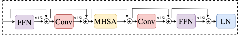
Figure 1: Overview of the proposed conformer block.

3 Speaker Adaptation

The main goal of speaker adaptation is to reduce the mismatch between train and test data by adapting the model to the unseen speakers of the test data. In this way, these methods adapt the speaker-independent model to be more robust to different speakers observed in the test data. In this work, we focus on feature-space adaptation methods.

Feature-space methods adapt the features of the network to be speaker-dependent. I-vectors [12] have been successfully applied to NN-based ASR systems [10, 23]. However, the integration of such vectors depends on the model architecture itself and it is not always clear what is the best way to do such an integration. For the BLSTM model, it was observed that concatenating the i-vectors to the network features gives significant improvement [24]. But this did not work well for the conformer model as observed in [9]. In this work, we investigate and propose better ways to integrate the i-vectors into the conformer AM. We develop a method to combine i-vectors into the MHSA module of the conformer AM which gives the best improvement.

Let $z_{1}^{T}$ be the input to a module in some conformer block (more details can be found in Section 5.2), and let $v$ represents a speaker representation vector such as i-vector or x-vector for the input utterance. The methods to integrate $v$ into the network can be defined as:

• Concat: concatenate the hidden representation $z_{t}$ with $v$

  $$\tilde{z}_{t}=[z_{t};v]\quad\forall t\in[1,T]$$ (1)

• Simple-Add: $U$ and $b$ are trainable parameters.

  $$\tilde{z}_{t}=z_{t}+Uv+b\quad\forall t\in[1,T]$$ (2)

• Complex-Add: $W$, $U$, and $b$ are trainable parameters.

  $$\tilde{z}_{t}=Wz_{t}+Uv+b\quad\forall t\in[1,T]$$ (3)

• Gated-Add: learn a scale and shift parameters conditioned on the speaker information $v$ [25, 26].

  $$\tilde{z}_{t} =z_{t}\otimes\gamma+\beta\quad\forall t\in[1,T]$$ (4)

  $$\gamma =\text{tanh}(Wv)+b_{1}$$ (5)

  $$\beta =\text{tanh}(Uv)+b_{2}$$ (6)

  where $W,U,b_{1},b_{2}$ are trainable parameters.

• Weighted-Simple-Add: The idea is to compute a score between each hidden representation $z_{t}$ and the speaker representation vector $v$. Sigmoid function is used to get a score between 0 and 1. Inspired from [19], we also apply a threshold $k$ on the learned weights. We use a value of 0.4 for $k$.

  $$w_{t} =\sigma(z_{t}\cdot(\text{tanh}(W\cdot v)+b_{1}))\in\mathbb{R}$$ (7)

  $$w_{t} =\begin{cases}w_{t},&w_{t}\geq k\\ 0,&w_{t}<k\end{cases}$$ (8)

  $$\tilde{z}_{t} =z_{t}+w_{t}\odot(Uv+b_{2})\quad\forall t\in[1,T]$$ (9)

  where $\sigma$ is the sigmoid function. $\cdot$ and $\odot$ are the dot-product and element-wise product operations respectively. $W$, $U$, $b_{1}$, and $b_{2}$ are trainable parameters.

Note that the representation capability (learnable space of parameters) is almost similar in nature between methods Concat, Simple-Add, and Complex-Add (see Section 5.2).

4 Experimental Setup

Experiments are conducted on the Switchboard 300h dataset [27] which consists of English telephony conversations. We use Hub5’00 as a development set for tuning the search hyperparameters. It consists of both Switchboard (SWB) and CallHome (CH) parts. CH part is much noisier. We use Hub5’01 as test set. RETURNN [28] is used to train the acoustic models and RASR [29] is used for decoding. All our configs files and code to reproduce our results can be found online.

4.1 Baseline

We use the baseline from our previous work [1]. It has 12 conformer blocks and we do time down-sampling by a factor of 3. Up-sampling is applied to the output layer using transposed convolution [30] to match the target fixed alignment. The total number of parameters is 88M. More details regarding hyperparameters and training methods can be found in [1]. We noticed that the momentum and epsilon parameters used in the BN layer were not optimal. After updating these parameters, our baseline achieves now WER of $11.7\%$ on Hub5’00. The details for applying speaker adaptation are explained in Section 5.2.

4.2 I-vectors Extraction

Our i-vector extraction pipeline follows the recipe described in [24]. To train the universal background model (UBM), 40-dimensional Gammatone features [31] with a context of 9 frames are concatenated and then reduced to a dimension of 60 using linear discriminant analysis (LDA). Normalization and LDA are usually applied after the extraction. We do not scale the i-vectors as done in [24] since we found this is crucial to get improvement. The same observation is also stated in [32]. For the final LDA dimension reduction, we have compared using i-vectors with dimensions 100, 200, and 300. Using 200-dimensional i-vectors is the best for our settings.

4.3 Sequence Discriminative Training (seq. train)

We use the lattice-based version of state-level minimum Bayes risk (sMBR) criterion [33]. The lattices are generated using a bigram LM. A small constant learning rate with value 1e-5 is used. At the final output layer, we use CE loss smoothing with a factor of 0.1. The sMBR loss scale is set to 0.9.

4.4 Language Models

In recognition, we use 4-gram count-based language model (LM) and LSTM LM as first pass decoding [34]. The LSTM LM has 51.3 perplexity (PPL) on Hub5’00 dataset. We use a transformer (Trafo) LM for lattice rescoring having PPL of 48.1 on Hub5’00 dataset.

5 Experimental Results

5.1 Improved Baseline

Our conformer acoustic model training recipe is built on top of our previous work [1]. The improved results are reported in Table 1. We replace BN with LN for all convolution modules. This also makes the model fits better for streaming mode. This leads to $3\%$ relative improvement in terms of WER on Hub5’00. Moreover, we study the effect of adding another convolution module in each conformer block following the Macaron style as suggested in [8]. This improves the system by $4\%$ relative in terms of WER on Hub5’00. In addition, we reduce the number of parameters by $40\%$ relative which makes training more efficient and requires less memory usage. To achieve that, we use an attention dimension of value 384 with 6 attention heads. The dimension of the feed-forward module is 1536. We also remove LongSkip [1]. The total number of parameters is then only 58M . The initial learning value is set to 1e-5. We apply linear warmup over 5 epochs with a peak learning rate of 8e-4. Table 2 shows that the improved baseline with reduced dimensions is $27\%$ relatively faster in terms of training speed.

Table 1: WERs [%] of improved baseline. 4-gram LM is used for recognition.

Model	Params. $[\text{M}]$	WER [%]
		Hub5’00
		SWB	CH	Total
Baseline	88	8.0	15.4	11.7
+LN instead of BN		7.7	15.1	11.4
+Two Conv modules	98	7.3	14.7	11.0
+Reduced dim.	58	7.1	14.3	10.7

Table 2: Comparison of training speed between the baseline conformer AM and the reduced dimension one. Training time is reported in hours for 1 epoch using single GeForce GTX 1080 Ti GPU.

Model	Train time [h]
Baseline	5.5
+Reduced dim.	4.0

5.2 Speaker Adaptation Results

We use the best conformer AM as described in Section 5.1 for speaker adaptive training (SAT). We apply SAT by integrating i-vectors into the network. We load the pretrained model and continue training with i-vectors while adapting SpecAugment and applying learning rate reset to escape from a local optimum as described in [2]. We also do not apply any learning rate warmup because we start from a pretrained model.

In Table 3, we compare different methods to integrate i-vectors into the conformer AM which are described in Section 3. First, we can observe that we get more improvement on CH part compared to SWB part since CH part is much noisier and contains more unseen speakers. We can observe that Weighted-Simple-Add gives the larger improvement. Using this method, we achieve $3.5\%$ relative improvement in terms of WER on CH part of Hub5’00 and $3\%$ relative improvement overall. On SWB part, all methods give a similar improvement which is only $0.1\%$ absolute.

For all SAT methods, we integrate the i-vectors into the first conformer block. In Table 4, we compare integrating i-vectors at different blocks of the conformer where Block 0 refers to the front-end VGG network. We can observe that integrating i-vectors at the first conformer block gives the best improvement and the performance degrades as we use deeper blocks. We can also observe that integrating at many blocks at the same time does not help. These results are done using the best method Weighted-Simple-Add.

Furthermore, we integrate i-vectors into the input of the MHSA module of the first conformer block. This means $z_{t}$ in the equations of Section 3 represents the input to the MHSA module. We decide to use this module since it captures global context which can potentially carry more speaker information. To measure this experimentally, we report in Table 5 the speaker error rates when adding a speaker identification loss on top of each module in the first conformer block. We can observe that the largest relative improvement is achieved at MHSA module. The settings for speaker identification experiments are described in Section 6.

Table 3: WERs [%] of speaker adaptive training by using i-vectors with different integration methods. 4-gram LM is used for recognition.

Integration method	WER [%]
	Hub5’00
	SWB	CH	Total
-	7.1	14.3	10.7
Concat	7.0	14.1	10.6
Simple-Add	7.0	14.0	10.5
Complex-Add	7.0	14.0	10.5
Gated-Add	7.0	14.2	10.6
Weighted-Simple-Add	7.0	13.8	10.4

Table 4: WERs [%] of speaker adaptive training by integrating i-vectors with Weighted-Simple-Add method at different conformer blocks. ”(*)” means using multiple blocks. 4-gram LM is used for recognition.

Block	WER [%]
	Hub5’00
	SWB	CH	Total
0	7.1	14.2	10.7
1	7.0	13.8	10.4
2	7.1	14.1	10.6
3	7.2	14.2	10.7
(1,2)	7.1	14.0	10.5
(1,2,3)	7.2	14.3	10.7

Table 5: Speaker identification error rates using the output of different modules in the first conformer block.

Module	Error [%]
1 FFN	31.7
1 Conv	28.6
MHSA	20.9
2 Conv	19.6
2 FFN	18.9

5.3 Comparison between i-vector and x-vector

The x-vectors are generated following the TDNN architecture in [13]. The training data is split into train and dev sets. We use attentive pooling [35] instead of statistical pooling which improves the speaker identification accuracy from $87.5\%$ to $93.2\%$ on the dev set. The comparison between using i-vectors and x-vectors for speaker adaptation using Weighted-Simple-Add method is reported in Table 6. Using x-vectors did not improve the performance but instead, lead to minor degradation on CH part. On possible explanation is that x-vectors mainly focus on the speaker characteristics whereas i-vectors are designed to capture both speaker and channel characteristics which might be important in this case [26]. Further investigations are needed for experiments with x-vectors.

Table 6: WERs [%] of comparison between i-vectors and x-vectors for speaker adaptation using Weighted-Simple-Add integration method. 4-gram LM is used for recognition.

Embedding	WER [%]
	Hub5’00
	SWB	CH	Total
i-vector	7.0	13.8	10.4
x-vector	7.0	14.4	10.7

5.4 Overall Results

We summarize our results in Table 7 and compare with different modeling approaches and architectures from the literature. Compared to our previous work [1], this work achieves $11.0\%$ and $4.1\%$ relative improvement with transformer LM on Hub5’00 and Hub5’01 datasets respectively. Moreover, our model outperforms a well-optimized BLSTM attention system [36] by $3\%$ and $5\%$ with LSTM LM on Hub5’00 and Hub5’01 datasets respectively. In addition, our model outperforms the TDNN baseline by $9\%$ relative on Hub5’00 dataset. Our best conformer AM is still behind the state-of-the-art results but not with a big margin. We argue that our baseline can be further improved by applying speed perturbation [36] and also longer training. Surprisingly, sequence training only give minor improvement which requires further investigation.

Table 7: Overall WER [%] comparison with literature.

Work	Approach	AM	LM	seq. train	ivec.	WER [%]
						Hub5’00			Hub 5’01
						SWB	CH	Total
[37]	Hybrid	TDNN	RNN	yes	yes	7.2	13.6	10.4	-
[1]	Hybrid	Conf.	LSTM	yes	no	6.9	14.5	10.7	10.1
			Trafo			6.6	14.1	10.3	09.7
[38]	RNN-T	LSTM	LSTM	no	yes	6.3	13.1	09.7	10.1
[36]	LAS	LSTM	LSTM	no	no	6.5	13.0	09.8	10.1
[9]	LAS	Conf.	-	no	yes	6.7	13.0	09.9	10.1
			LSTM			5.7	11.4	08.6	08.5
			Trafo			5.5	11.2	08.4	08.5
this work	Hybrid	Conf.	4-gram	no	no	7.1	14.3	10.7	11.0
					yes	7.0	13.8	10.4	10.5
				yes		7.1	13.5	10.3	10.4
			LSTM			6.5	12.5	09.5	09.6
			Trafo			6.3	12.1	09.2	09.3

6 Speaker Identification Error Analysis

It has been observed empirically that the improvement by speaker adaptation is not significant when using a conformer-based AM [9]. However, BLSTM-based AMs benefit much more from speaker adaptation [24]. We argue that the reason behind this is that the conformer model is able to better learn speaker information in the lower layers which make it already robust to different speakers. To verify this, we conduct the following experiment using the Switchboard 300h training dataset. We added a speaker identification loss on top of the output of each layer for both the conformer model and BLSTM model. The BLSTM model consists of 6 layers following [1, 24]. Then, we freeze all the AM parameters except the speaker identification loss parameters. We use an attention mechanism as [39] to get a soft speaker representation from the last output layer of the AM. This can also learn to skip unnecessary information such as silence. The total number of speakers is 520. We split the training dataset into train and dev parts. The speaker identification error rates on the dev set are reported in Figure 2. We can observe that the conformer model has a much better speaker identification accuracy using the lower layers compared to the BLSTM model. It was able to achieve using the second block a speaker identification error rate of $13\%$ while the lowest error rate that the BLSTM achieves is $43\%$. These figures also show that lower layers are more important for learning speaker representations. For the conformer, we also observe that having the speaker loss on top of the MHSA module is enough to achieve such a low speaker error rate. This also explains why the proposed method to integrate the i-vectors into the MHSA module works the best for us. Moreover, the speaker error starts to increase for higher layers which is most probably because the model starts to filter out unnecessary speaker information to learn high-level features.

Figure 2: Speaker identification error rates using BLSTM AM and conformer AM. Layer depth refers to the layer index divided by total number of layers.

7 Conclusions & Future Work

In this work, we improved our training recipe for conformer-based hybrid Neural Network-Hidden Markov Model. We achieved $11\%$ relative improvement in terms of word-error-rate (WER) on the Switchboard 300h Hub5’00 dataset. We also developed an efficient training recipe with $34\%$ relative reduction in total number of parameters. Moreover, we investigated different ways to apply speaker adaptive training (SAT) for conformer-based acoustic models. We propose a method, called Weighted-Simple-Add to add weighted speaker information vectors to the input of multi-head self-attention module of the conformer AM. Using this method for SAT, we achieve $3.5\%$ and $4.5\%$ relative improvement in terms of WER on the CallHome part of Hub5’00 and Hub5’01 respectively. We also perform some analysis and showed that the conformer-based AM is already good enough for speaker identification task. For future work, we plan to apply our recipe to a noisier dataset such as CHiME-4 [40] as well as applying model-space SAT approaches [41].

8 Acknowledgements

This work was partially supported by the project HYKIST funded by the German Federal Ministry of Health on the basis of a decision of the German Federal Parliament (Bundestag) under funding ID ZMVI1-2520DAT04A. We thank Wilfried Michel, Zoltán Tüske, and Wei Zhou for useful discussions. We also thank Alexander Gerstenberger for performing lattice rescoring with Transformer.

References

- [1] M. Zeineldeen, J. Xu, C. Lüscher, W. Michel, A. Gerstenberger, R. Schlüter, and H. Ney, “Conformer-based Hybrid ASR System for Switchboard Dataset,” in ICASSP, Singapore, May 2022, pp. 7437–7441.
- [2] W. Zhou, W. Michel, K. Irie, M. Kitza, R. Schlüter, and H. Ney, “The RWTH ASR System for TED-LIUM Release 2: Improving Hybrid HMM with SpecAugment,” in ICASSP, Barcelona, Spain, May 2020, pp. 7839–7843.
- [3] C. Lüscher, E. Beck, K. Irie, M. Kitza, W. Michel, A. Zeyer, R. Schlüter, and H. Ney, “RWTH ASR Systems for LibriSpeech: Hybrid vs Attention,” in INTERSPEECH, Graz, Austria, Sep. 2019, pp. 231–235.
- [4] S. Hochreiter and J. Schmidhuber, “Long Short-term Memory,” Neural Computation, vol. 9, no. 8, pp. 1735–1780, 1997.
- [5] O. Abdel-Hamid, A. Mohamed, H. Jiang, L. Deng, G. Penn, and D. Yu, “Convolutional Neural Networks for Speech Recognition,” IEEE/ACM Transactions on Audio, Speech, and Language Processing, vol. 22, no. 10, pp. 1533–1545, 2014.
- [6] V. Peddinti, D. Povey, and S. Khudanpur, “A Time Delay Neural Network Architecture for Efficient Modeling of Long Temporal Contexts,” in INTERSPEECH, Dresden, Germany, Sep. 2015, pp. 3214–3218.
- [7] M. Sperber, J. Niehues, G. Neubig, S. Stüker, and A. Waibel, “Self-Attentional Acoustic Models,” in INTERSPEECH, Hyderabad, India, Sep. 2018, pp. 3723–3727.
- [8] A. Gulati, J. Qin, C. Chiu, N. Parmar, Y. Zhang, J. Yu, W. Han, S. Wang, Z. Zhang, Y. Wu, and R. Pang, “Conformer: Convolution-augmented Transformer for Speech Recognition,” in INTERSPEECH, Shanghai, China, Oct. 2020, pp. 5036–5040.
- [9] Z. Tüske, G. Saon, and B. Kingsbury, “On the Limit of English Conversational Speech Recognition,” in INTERSPEECH, Brno, Czechia, Sep. 2021, pp. 2062–2066.
- [10] G. Saon, H. Soltau, D. Nahamoo, and M. Picheny, “Speaker Adaptation of Neural Network Acoustic Models Using I-Vectors,” in ASRU, Olomouc, Czech Republic, Dec. 2013, pp. 55–59.
- [11] C. Leggetter and P. Woodland, “Maximum Likelihood Linear Regression for Speaker Adaptation of Continuous Density Hidden Markov Models,” Computer Speech & Language, vol. 9, no. 2, pp. 171–185, 1995. [Online]. Available: https://www.sciencedirect.com/science/article/pii/S0885230885700101
- [12] N. Dehak, P. J. Kenny, R. Dehak, P. Dumouchel, and P. Ouellet, “Front-End Factor Analysis for Speaker Verification,” IEEE Transactions on Audio, Speech, and Language Processing, vol. 19, no. 4, pp. 788–798, 2011.
- [13] D. Snyder, D. Garcia-Romero, G. Sell, D. Povey, and S. Khudanpur, “X-Vectors: Robust DNN Embeddings for Speaker Recognition,” in ICASSP, Calgary, Alberta, Canada, 2018, pp. 5329–5333.
- [14] F. Seide, G. Li, X. Chen, and D. Yu, “Feature Engineering in Context-dependent Deep Neural Networks for Conversational Speech Transcription,” in ASRU, Waikoloa, HI, USA, 2011, pp. 24–29.
- [15] R. Gemello, F. Mana, S. Scanzio, P. Laface, and R. De Mori, “Adaptation of Hybrid ANN/HMM Models using Linear Hidden Transformations and Conservative Training,” in ICASSP, vol. 1. Toubouse, France: IEEE, May 2006, pp. I–I.
- [16] B. Li and K. C. Sim, “Comparison of Discriminative Input and Output Transformations for Speaker Adaptation in the Hybrid NN/HMM Systems,” in Eleventh Annual Conference of the International Speech Communication Association, Makuhari, Chiba, Japan, 2010.
- [17] H. Zhu, L. Wang, P. Zhang, and Y. Yan, “Multi-accent Adaptation Based on Gate Mechanism,” in INTERSPEECH, Graz, Austria, Sep. 2019, pp. 744–748.
- [18] X. Gong, Y. Lu, Z. Zhou, and Y. Qian, “Layer-wise Fast Adaptation for End-to-End Multi-accent Speech Recognition,” in INTERSPEECH, Brno, Czechia, 2021, pp. 1274–1278.
- [19] K. Deng, S. Cao, and L. Ma, “Improving Accent Identification and Accented Speech Recognition under a Framework of Self-supervised Learning,” in INTERSPEECH, Brno, Czechia, Sep. 2021, pp. 1504–1508.
- [20] M. A. T. Turan, E. Vincent, and D. Jouvet, “Achieving Multi-accent ASR via Unsupervised Acoustic Model Adaptation,” in INTERSPEECH, Shanghai, China, Oct. 2020, pp. 1286–1290.
- [21] S. Ioffe and C. Szegedy, “Batch Normalization: Accelerating Deep Network Training by Reducing Internal Covariate Shift,” in ICML, vol. 37, Lille, France, 2015, pp. 448–456.
- [22] L. J. Ba, J. R. Kiros, and G. E. Hinton, “Layer Normalization,” CoRR, vol. abs/1607.06450, 2016.
- [23] V. Peddinti, G. Chen, V. Manohar, T. Ko, D. Povey, and S. Khudanpur, “JHU ASpIRE System: Robust LVCSR with TDNNS, IVector Adaptation and RNN-LMS,” in ASRU. Scottsdale, AZ, USA: IEEE, Dec. 2015, pp. 539–546.
- [24] M. Kitza, P. Golik, R. Schlüter, and H. Ney, “Cumulative Adaptation for BLSTM Acoustic Models,” in INTERSPEECH, Graz, Austria, Sep. 2019, pp. 754–758.
- [25] S. Yoo, I. Song, and Y. Bengio, “A Highly Adaptive Acoustic Model for Accurate Multi-dialect Speech Recognition,” in ICASSP, Brighton, UK, May 2019, pp. 5716–5720.
- [26] J. Rownicka, P. Bell, and S. Renals, “Embeddings for DNN Speaker Adaptive Training,” in ASRU. Singapore: IEEE, Dec. 2019, pp. 479–486.
- [27] J. Godfrey, E. Holliman, and J. McDaniel, “Switchboard: Telephone Speech Corpus for Research and Development,” in ICASSP, vol. 1, San Francisco,USA, Mar. 1992, pp. 517–520.
- [28] A. Zeyer, T. Alkhouli, and H. Ney, “RETURNN as a Generic Flexible Neural Toolkit with Application to Translation and Speech Recognition,” in Annual Meeting of the Assoc. for Computational Linguistics, Melbourne, Australia, Jul. 2018.
- [29] S. Wiesler, A. Richard, P. Golik, R. Schlüter, and H. Ney, “RASR/NN: The RWTH Neural Network Toolkit for Speech Recognition,” in ICASSP, Florence, Italy, May 2014, pp. 3313–3317.
- [30] J. Long, E. Shelhamer, and T. Darrell, “Fully Convolutional Networks for Semantic Segmentation,” in CVPR, Boston, USA, Jun. 2015, pp. 3431–3440.
- [31] R. Schluter, I. Bezrukov, H. Wagner, and H. Ney, “Gammatone Features and Feature Combination for Large Vocabulary Speech Recognition,” in ICASSP, Honolulu, USA, Apr. 2007, pp. 649–652.
- [32] A. Rouhe, T. Kaseva, and M. Kurimo, “Speaker-aware Training of Attention-based End-to-end Speech Recognition Using Neural Speaker Embeddings,” in ICASSP, Barcelona, Spain, May 2020, pp. 7064–7068.
- [33] M. Gibson and T. Hain, “Hypothesis Spaces for Minimum Bayes Risk Training in Large Vocabulary Speech Recognition,” in INTERSPEECH, Pittsburgh, USA, Sep. 2006.
- [34] E. Beck, W. Zhou, R. Schlüter, and H. Ney, “LSTM Language Models for LVCSR in First-pass Decoding and Lattice-Rescoring,” CoRR, vol. abs/1907.01030, 2019. [Online]. Available: http://arxiv.org/abs/1907.01030
- [35] K. Okabe, T. Koshinaka, and K. Shinoda, “Attentive Statistics Pooling for Deep Speaker Embedding,” in INTERSPEECH, Hyderabad, India, Sep. 2018, pp. 2252–2256.
- [36] Z. Tüske, G. Saon, K. Audhkhasi, and B. Kingsbury, “Single Headed Attention Based Sequence-to-sequence Model for State-of-the-Art Results on Switchboard,” in INTERSPEECH, Shanghai, China, Sep. 2020, pp. 551–555.
- [37] S. Hu, X. Xie, S. Liu, J. Yu, Z. Ye, M. Geng, X. Liu, and H. Meng, “Bayesian Learning of LF-MMI Trained Time Delay Neural Networks for Speech Recognition,” IEEE/ACM Transactions on Audio, Speech, and Language Processing, vol. 29, pp. 1514–1529, 2021.
- [38] G. Saon, Z. Tüske, D. Bolaños, and B. Kingsbury, “Advancing RNN Transducer Technology for Speech Recognition,” in ICASSP. Toronto, Canada: IEEE, 2021, pp. 5654–5658.
- [39] S. Sigtia, E. Marchi, S. Kajarekar, D. Naik, and J. Bridle, “Multi-Task Learning for Speaker Verification and Voice Trigger Detection,” in ICASSP. Barcelona, Spain: IEEE, May 2020, pp. 6844–6848.
- [40] Y. Yang, P. Wang, and D. Wang, “A Conformer Based Acoustic Model for Robust Automatic Speech Recognition,” CoRR, vol. abs/2203.00725, 2022. [Online]. Available: https://doi.org/10.48550/arXiv.2203.00725
- [41] M. Kitza, R. Schlüter, and H. Ney, “Comparison of BLSTM-layer-specific Affine Transformations for Speaker Adaptation,” in INTERSPEECH, Hyderabad, India, Sep. 2018, pp. 877–881.