Wiener Graph Deconvolutional Network Improves Graph Self-Supervised Learning

Abstract

Graph self-supervised learning (SSL) has been vastly employed to learn representations from unlabeled graphs. Existing methods can be roughly divided into predictive learning and contrastive learning, where the latter one attracts more research attention with better empirical performance. We argue that, however, predictive models weaponed with powerful decoder could achieve comparable or even better representation power than contrastive models. In this work, we propose a Wiener Graph Deconvolutional Network (WGDN), an augmentation-adaptive decoder empowered by graph wiener filter to perform information reconstruction. Theoretical analysis proves the superior reconstruction ability of graph wiener filter. Extensive experimental results on various datasets demonstrate the effectiveness of our approach.

1 Introduction

Self-Supervised Learning (SSL), which extracts informative knowledge through well-designed pretext tasks from unlabeled data, has been extended to graph data recently due to its great success in computer vision (CV) (He et al. 2020) and natural language processing (NLP) (Devlin et al. 2019). With regard to the objectives of pretext tasks, graph SSL can be divided into two major categories: predictive SSL and contrastive SSL (Liu et al. 2022). Predictive models learn informative properties generated from graph freely via prediction tasks, while contrastive models are trained on the mutual information between different views augmented from the original graph. As the dominant technique, contrastive SSL has achieved state-of-the-art performance empirically (Xu et al. 2021; Thakoor et al. 2022; Lee, Lee, and Park 2022) for graph representation learning. In contrast, the development of predictive SSL has lagged behind over the past few years.

Graph reconstruction is a natural self-supervision, and thus most methods in predictive SSL employ graph autoencoder (GAE) as their backbones (Wang et al. 2017; Hu et al. 2020b; Li et al. 2020b). The work of GraphMAE (Hou et al. 2022) re-validates the potentials of reconstruction paradigm. Despite recent advancements, the importance of graph decoder has been largely ignored. Most existing works leverage trivial decoders, such as multi-layer perceptron (MLP) (Kipf and Welling 2016; Pan et al. 2018; You et al. 2020b), which under-exploit graph topology information, and thus may lead to the degradation in learning capability. Vanilla graph neural networks (GNNs), such as GCN (Kipf and Welling 2017), are inappropriate for decoding due to their Laplacian-smooth essence. To overcome such inherent limitation of GCN, GALA (Park et al. 2019) adopts spectral counterpart of GCN to facilitate the learning, but may take the risk of unstable learning due to its poor resilience to data augmentation (See Figure 1). GAT (Veličković et al. 2018) is employed as decoder in recent works including GATE (Salehi and Davulcu 2020) and GraphMAE (Hou et al. 2022). Although attention mechanism enhances model flexibility, recent work (Balcilar et al. 2021) shows GAT acts like a low-pass filter and cannot well reconstruct the graph spectrum. As an inverse to GCN (Kipf and Welling 2017), graph deconvolutional network (GDN) could be expected to further boost the performance of reconstruction (Li et al. 2021), which may substantially benefit the context of representation learning. We present a summary of different decoders of predictive graph SSL in Table 1. Given the aforementioned observations, a natural question comes up, that is, can we improve predictive SSL by a framework with powerful decoder?

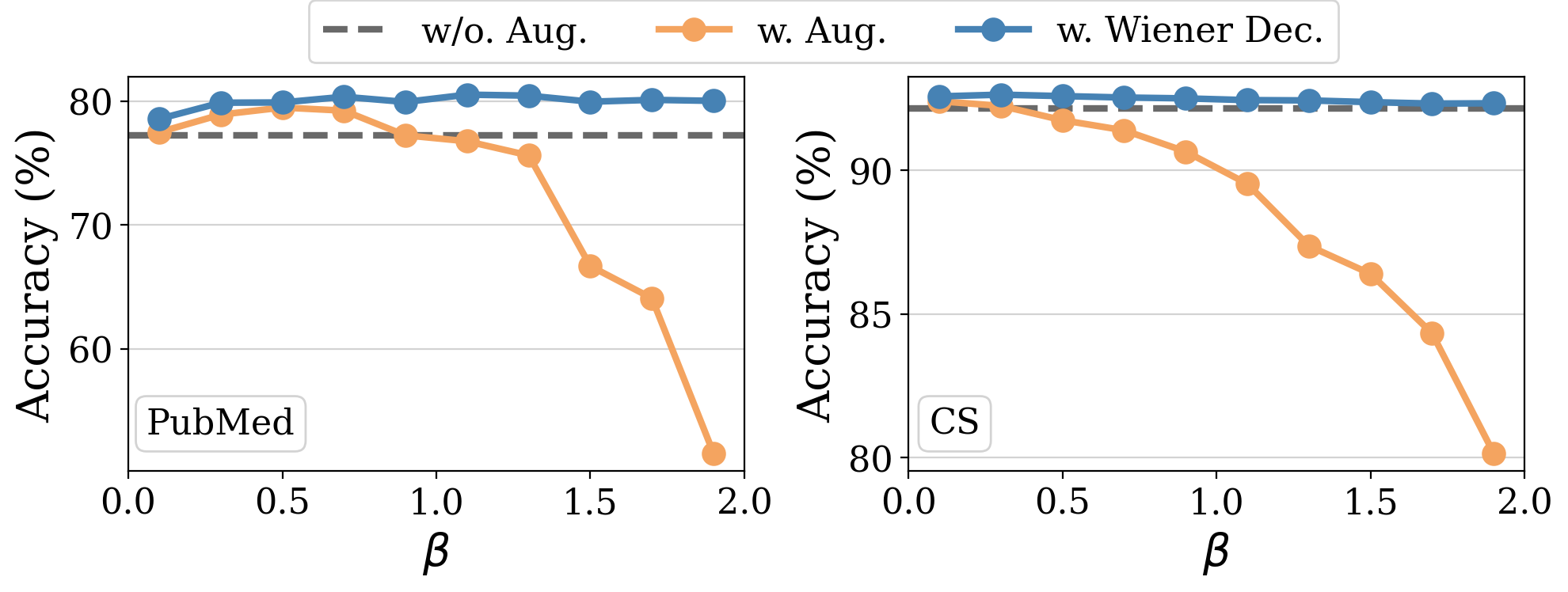
Figure 1: Comparison of different variants of GALA against latent Gaussian augmentation with magnitude $\beta$.

Model	Decoder	Feature	Structure	Deconv.	Augmentation	Spectral	Space
		Loss	Loss	Decoder	Adaption	Kernel
VGAE (Kipf and Welling 2016)	DP	-	CE	✗	✗	✗	$\mathcal{O}(N^{2})$
ARVGA (Pan et al. 2018)	DP	-	CE	✗	✗	✗	$\mathcal{O}(N^{2})$
MGAE (Wang et al. 2017)	MLP	MSE	-	✗	✗	✗	$\mathcal{O}(N)$
AttrMask (Hu et al. 2020b)	MLP	CE	-	✗	✗	✗	$\mathcal{O}(N)$
GALA (Park et al. 2019)	GNN	MSE	-	✓	✗	✗	$\mathcal{O}(N)$
GraphMAE (Hou et al. 2022)	GNN	SCE	-	✗	✓	✗	$\mathcal{O}(N)$
WGDN	GNN	MSE	-	✓	✓	✓	$\mathcal{O}(N)$

Table 1: Technical components comparison within predictive SSL approaches. DP: Non-parametric Dot Product. CE: Cross-Entropy Error. MSE: Mean Square Error. SCE: Scaled-Cosine Error.

Typically, a powerful decoder should at least remain effective against augmentations. Motivated by recent advancement of wiener in deep image reconstruction (Dong, Roth, and Schiele 2020), we introduce the classical deconvolutional technique, wiener filter, into GDN, which is the theoretical optimum for restoring augmented signals with respect to mean square error (MSE). We propose a GAE framework (Li et al. 2020b), named Wiener Graph Deconvolutional Network (WGDN), which utilizes graph wiener filter to facilitate representation learning with graph spectral kernels. We first derive the graph wiener filter and prove its superiority in theory. We observe that, however, directly using the explicit graph wiener filter induces low scalability due to indispensable eigen-decomposition and may not be applicable to large-scale datasets. Therefore, we adopt average graph spectral energy and Remez polynomial (Pachon and Trefethen 2009) for fast approximation.

We evaluate the learned representation quality on two downstream tasks: node classification and graph classification. Empirically, our proposed WGDN achieves better results over a wide range of state-of-the-art benchmarks of graph SSL with efficient computational cost. Particularly, WGDN yields up to 1.4% higher accuracy than runner-up model, and requires around 30% less memory overhead against the most efficient contrastive counterpart.

2 Related Work

Graph self-supervised learning.

According to recent surveys (Liu et al. 2022; Xie et al. 2022), works in graph SSL can be classified into two categories: contrastive learning and predictive learning. Contrastive SSL attracts more attention currently due to the state-of-the-art performance on representation learning. Early efforts focus on the design of negative sampling and augmentation schemes, such as corruptions in DGI (Veličković et al. 2019), graph diffusion in MVGRL (Hassani and Khasahmadi 2020) and masking in GRACE (Zhu et al. 2020) and GCA (Zhu et al. 2021). Recent works have attempted for negative-sample-free contrastive SSL. For example, BGRL (Thakoor et al. 2022) adapts BYOL (Grill et al. 2020) for graph representation learning, CCA-SSG (Zhang et al. 2021) conducts feature decorrelation, and AFGRL (Lee, Lee, and Park 2022) obtains positive pairs via latent space clustering. Despite their advancement, intricate architecture designs are required.

As for predictive learning, predicting node features and neighborhood context is a traditional pretext task with graph autoencoder (GAE). For instance, VGAE (Kipf and Welling 2016) and ARVGA (Pan et al. 2018) learn missing edges prediction by structural reconstruction. Moreover, one representative manner (You et al. 2020b) follows the perturb-then-learn strategy to predict the corrupted information, such as attribute masking  (Hu et al. 2020b) and feature corruption  (Wang et al. 2017). Recently, GraphMAE (Hou et al. 2022) implements a masking strategy and scaled cosine error for feature reconstruction and achieves great success to match state-of-the-art contrastive SSL approaches. However, it ignores the potential benefit leveraging graph spectral theory. In this work, we propose an augmentation-adaptive GAE framework that unleashes the power of graph spectral propagation.

Graph deconvolutional network.

Regarding graph deconvolution, early research (Yang and Segarra 2018) formulates the deconvolution as a pre-processing step. GALA (Park et al. 2019) performs Laplacian sharpening to recover information. Recent work (Zhang et al. 2020) employs GCN (Kipf and Welling 2017) to reconstruct node features from the latent representations. All these works, however, neglect the influence of augmentation. Another GDN framework (Li et al. 2021) is designed via a combination of inverse filters in spectral domain and denoising layers in wavelet domain, which is sub-optimal regarding signal reconstruction. Wiener filtering, as an alternative, executes an optimal trade-off between signal recovering and denoising. It has been introduced to deconvolutional networks (Dong, Roth, and Schiele 2020; Son and Lee 2017) for image deblurring. However, its effectiveness on graph structure has not been well investigated yet.

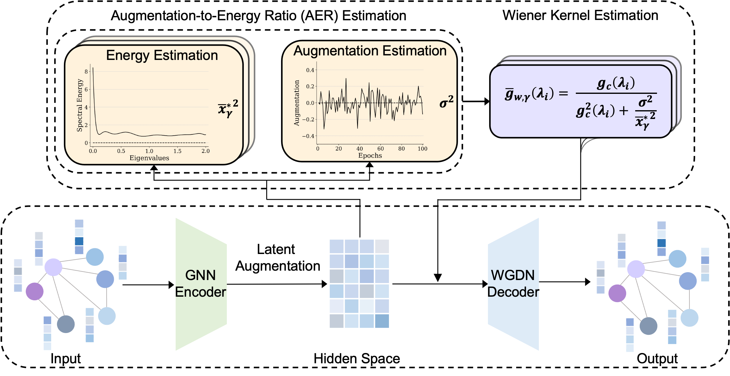
Figure 2: The autoencoder framework of WGDN for graph SSL. Given the augmented latent representations, graph wiener filter is approximated via estimating spectral energy and augmentations adaptively. With such, WGDN permits the stable feature reconstruction from the augmented latent space for representation learning.

3 Preliminaries

Under a generic self-supervised graph representation learning setup, we are given an attributed graph $\mathcal{G}=(\mathcal{V},\mathbf{A},\mathbf{X})$ consisting of: (1) $\mathcal{V}=\{v_{1},v_{2},...,v_{N}\}$ is the set of nodes; (2) $\mathbf{A}\in\mathbb{R}^{N\times N}$ is the adjacency matrix where $\mathbf{A}_{ij}\in\{0,1\}$ represents whether an undirected edge exists between $v_{i}$ and $v_{j}$; and (3) $\mathbf{X}\in\mathbb{R}^{N\times D}$ denotes the feature matrix. Our objective is to learn an autoencoder with encoder $\mathcal{E}:(\mathbb{R}^{N\times N},\mathbb{R}^{N\times D})\mapsto\mathbb{R}^{N\times D^{\prime}}$ and decoder $\mathcal{D}:\mathbb{R}^{N\times D^{\prime}}\mapsto\mathbb{R}^{N\times D}$ to produce node embedding, or graph embedding upon a pooling function. $\mathbf{H}=\mathcal{E}(\mathbf{A},\mathbf{X})\in\mathbb{R}^{N\times D^{\prime}}$ represents the learned embedding in low dimensional space, which can be used for various downstream tasks.

Graph convolution.

Convolutional operation in graph can be interpreted as a special form of Laplacian smoothing on nodes. From the spectral perspective, graph convolution on a signal $\mathbf{x}\in\mathbb{R}^{N}$ with a filter $g_{c}$ is defined as

$$\mathbf{h}=g_{c}\ast\mathbf{x} =\mathbf{U}\text{diag}(g_{c}(\lambda_{1}),...,g_{c}(\lambda_{N}))\mathbf{U}^{T}\mathbf{x}$$ (1)

$$=\mathbf{U}g_{c}(\mathbf{\Lambda})\mathbf{U}^{T}\mathbf{x}=g_{c}(\mathbf{L})\mathbf{x},$$

where $\{\lambda_{i}\}_{i=1}^{N}$ and $\mathbf{U}$ represent the eigenvalues and eigenvectors of normalized Laplacian matrix $\mathbf{L}=\mathbf{I}-\mathbf{D}^{-\frac{1}{2}}\mathbf{A}\mathbf{D}^{-\frac{1}{2}}=\mathbf{U}\mathbf{\Lambda}\mathbf{U}^{T}$ respectively. $\mathbf{D}$ denotes the Degree matrix. $\ast$ denotes convolutional operator. We consider (1) GCN (Kipf and Welling 2017), it is a low-pass filter in spectral domain with $g_{c}(\lambda_{i})=1-\lambda_{i}$ shown by (Wu et al. 2019); (2) GDC (Klicpera, Weißenberger, and Günnemann 2019) and Heatts (Li et al. 2020a), both use heat kernel $g_{c}(\lambda_{i})=e^{-t\lambda_{i}}$; (3) APPNP (Gasteiger, Bojchevski, and Günnemann 2019), it leverages personalized pagerank (PPR) kernel $g_{c}(\lambda_{i})=\frac{\alpha}{1-(1-\alpha)(1-\lambda_{i})}$.

Graph deconvolution.

As an inverse to convolution, graph deconvolution aims to recover the input attributes given the smoothed node representation. From the spectral perspective, graph deconvolution on a smoothed representation $\mathbf{h}\in\mathbb{R}^{N}$ with filter $g_{d}$ is defined as

$$\hat{\mathbf{x}}=g_{d}\ast\mathbf{h} =\mathbf{U}\text{diag}(g_{d}(\lambda_{1}),...,g_{d}(\lambda_{N}))\mathbf{U}^{T}h$$ (2)

$$=\mathbf{U}g_{d}(\mathbf{\Lambda})\mathbf{U}^{T}\mathbf{h}=g_{d}(\mathbf{L})\mathbf{h}.$$

A trivial selection of $g_{d}$ is the inverse function of $g_{c}$, e.g., $g_{d}(\lambda_{i})=\frac{1}{1-\lambda_{i}}$ for GCN (Li et al. 2021), $g_{d}(\lambda_{i})=e^{t\lambda_{i}}$ for heat kernel, or $g_{d}(\lambda_{i})=\frac{1-(1-\alpha)(1-\lambda_{i})}{\alpha}$ for PPR kernel.

4 The proposed framework

In this section, we first extend classical wiener filter to graph domain and demonstrate its superiority in reconstructing graph features. Then, we propose Wiener Graph Deconvolutional Network (WGDN), an efficient and augmentation-adaptive framework empowered by graph wiener filter.

4.1 Wiener filter on graph

In this work, we follow the settings in previous papers (Jin and Zhang 2019; Cheung and Yeung 2021) and introduce additive latent augmentations in model training due to its flexible statistical characteristics, such as unbiasedness and covariance-preserving (Zhang et al. 2022). Combining with the graph convolution in Eq. 1, augmented representation $\hat{\mathbf{h}}$ in graph is similarly defined as

$$\hat{\mathbf{h}}=\mathbf{U}g_{c}(\mathbf{\Lambda})\mathbf{U}^{T}\mathbf{x}+\mathbf{\epsilon},$$ (3)

where $\mathbf{x}\in\mathbb{R}^{N}$ denotes input features and $\mathbf{\epsilon}\in\mathbb{R}^{N}$ is assumed to be any i.i.d. random augmentation with $\mathbb{E}[\mathbf{\epsilon}_{i}]=0$ and $\mathbb{VAR}[\mathbf{\epsilon}_{i}]=\sigma^{2}$. In contrast to the isolated data augmentations in graph topology and features, $\epsilon$ indirectly represents joint augmentations to both (Jin and Zhang 2019). Naturally, feature recovered by graph deconvolution is formulated by

$$\hat{\mathbf{x}}=\mathbf{U}g_{d}(\mathbf{\Lambda})g_{c}(\mathbf{\Lambda})\mathbf{U}^{T}\mathbf{x}+\mathbf{U}g_{d}(\mathbf{\Lambda})\mathbf{U}^{T}\mathbf{\epsilon}.$$ (4)

Proposition 4.1.

Let $\hat{\mathbf{x}}_{inv}$ be recovered features by inverse filter $g_{d}(\lambda_{i})=g_{c}^{-1}(\lambda_{i})$. For common low-pass filters satisfying $g_{c}:[0,2]\mapsto[-1,1]$, such as GCN, Heat and PPR, the reconstruction MSE is dominated by amplified augmentation $\text{MSE}(\hat{\mathbf{x}}_{inv})=\mathbb{E}\norm{\mathbf{x}-\hat{\mathbf{x}}_{inv}}_{2}^{2}=\sum_{i=1}^{N}\frac{\sigma^{2}}{g_{c}^{2}(\lambda_{i})}$.

The proof is trivial and illustrated in Appendix A for details. Based on Proposition 4.1, feature reconstruction becomes unstable and even ineffective if augmentation exists. To well utilize the power of augmentation, our goal is to stabilize the reconstruction paradigm, which resembles the classical restoration problems. In signal deconvolution, classical wiener filter (Wiener 1964) is able to produce a statistically optimal estimation of the real signals from the augmented ones with respect to MSE. With this regard, we are encouraged to extend wiener filter to graph domain (Perraudin and Vandergheynst 2017). Assuming the augmentation to be independent from input features, graph wiener filter can be similarly defined by projecting MSE into graph spectral domain

$$\text{MSE}(\hat{\mathbf{x}})$$ (5)

$$=\mathbb{E}\norm{\hat{\mathbf{x}}-\mathbf{x}}_{2}^{2}=\mathbb{E}\norm{\mathbf{U}^{T}\hat{\mathbf{x}}-\mathbf{U}^{T}\mathbf{x}}_{2}^{2}$$

$$=\sum_{i=1}^{N}(g_{d}(\lambda_{i})g_{c}(\lambda_{i})-1)^{2}\mathbb{E}[x^{\ast 2}_{i}]+g_{d}^{2}(\lambda_{i})\mathbb{E}[\mathbf{\epsilon}^{\ast 2}_{i}]$$

$$=\sum_{i=1}^{N}S(\lambda_{i},x^{\ast}_{i},\sigma,g_{c},g_{d}),$$

where $\mathbf{x}^{\ast}=\mathbf{U}^{T}\mathbf{x}=\{x^{\ast}_{1},x^{\ast}_{2},...,x^{\ast}_{N}\}$ and $\mathbf{\epsilon}^{\ast}=\mathbf{U}^{T}\mathbf{\epsilon}=\{\epsilon^{\ast}_{1},\epsilon^{\ast}_{2},...,\epsilon^{\ast}_{N}\}$ represent graph spectral projection of the input and augmentation respectively. We denote $\mathbb{E}[x^{\ast 2}_{i}]$ and $S(\lambda_{i},x^{\ast}_{i},\sigma,g_{c},g_{d})$ as the spectral energy and spectral reconstruction error of spectrum $\lambda_{i}$. Considering the convexity of Eq. 5, MSE is minimized by setting the derivative with respect to $g_{d}(\lambda_{i})$ to zero and thus we obtain the graph wiener filter $g_{w}(\lambda_{i})$ as

$$g_{w}(\lambda_{i})=\frac{g_{c}(\lambda_{i})}{g_{c}^{2}(\lambda_{i})+\sigma^{2}/\mathbb{E}[x^{\ast 2}_{i}]},$$ (6)

where $\sigma^{2}=\mathbb{VAR}[\mathbf{\epsilon}^{\ast}_{i}]=\mathbb{E}[\mathbf{\epsilon}^{\ast 2}_{i}]$ and $\sigma^{2}/\mathbb{E}[x^{\ast 2}_{i}]$ is denoted as the Augmentation-to-Energy Ratio (AER) of particular spectrum $\lambda_{i}$, which represents the relative magnitude of augmentation.

Proposition 4.2.

Let $\hat{\mathbf{x}}_{w}$ be recovered features by $g_{w}(\lambda_{i})$, where $g_{w}(\lambda_{i})$ is a graph wiener filter, then the reconstruction MSE and variance of $\hat{\mathbf{x}}_{w}$ are less than $\hat{\mathbf{x}}_{inv}$.

Please refer to Appendix B for details. Proposition 4.2 shows graph wiener filter has better reconstruction property than inverse filter, which promotes the resilience to latent augmentations and permits stable model training. We observe that, in Eq. 2 and 6, eigen-decomposition is indispensable in computations of spectral energy and deconvolutional filter. However, in terms of scalability, an important issue for large-scale graphs is to avoid eigen-decomposition. Note that $\sum_{i=1}^{N}\mathbb{E}[x^{\ast 2}_{i}]=\sum_{i=1}^{N}\mathbb{E}[x^{2}_{i}]$ due to orthogonal transformation, we propose the modified graph wiener filter $\bar{g}_{w,\gamma}$ with average spectral energy $\bar{x}^{\ast 2}_{\gamma}=\gamma\cdot\bar{x}^{\ast 2}=\gamma\cdot\frac{1}{N}\sum_{i=1}^{N}\mathbb{E}[x^{\ast 2}_{i}]$ as

$$\bar{g}_{w,\gamma}(\lambda_{i})=\frac{g_{c}(\lambda_{i})}{g_{c}^{2}(\lambda_{i})+\sigma^{2}/\bar{x}^{\ast 2}_{\gamma}},$$ (7)

where $\gamma$ is a hyper-parameter to adjust AER. As a natural extension of Proposition 4.2, $\bar{g}_{w,\gamma}$ owns the following proposition.

Proposition 4.3.

Let $\hat{\mathbf{x}}_{w,\gamma}$ be the recovered features by modified graph wiener filter $\bar{g}_{w,\gamma}(\lambda_{i})$, then the variance of $\hat{\mathbf{x}}_{w,\gamma}$ is less than $\hat{\mathbf{x}}_{inv}$. In spectral domain, given two different $\gamma_{1}$, $\gamma_{2}$ such that $\mathbb{E}[x^{\ast 2}_{i}]\leq\bar{x}^{\ast 2}_{\gamma_{1}}\leq\bar{x}^{\ast 2}_{\gamma_{2}}$, the spectral reconstruction error $S(\lambda_{i},x^{\ast}_{i},\sigma,g_{c},\bar{g}_{w,\gamma_{1}})\leq S(\lambda_{i},x^{\ast}_{i},\sigma,g_{c},\bar{g}_{w,\gamma_{2}})\leq S(\lambda_{i},x^{\ast}_{i},\sigma,g_{c},g_{c}^{-1})$.

Please refer to Appendix C for details. Proposition 4.3 demonstrates that $\bar{g}_{w,\gamma}$ attends to spectral reconstructions over different ranges of spectra, depending on the selection of $\gamma$. The graph wiener kernel $\mathbf{D}_{\gamma}=\mathbf{U}\bar{g}_{w,\gamma}(\mathbf{\Lambda})\mathbf{U}^{T}$ can also be reformatted as matrix multiplication

$$\mathbf{D}_{\gamma}=\mathbf{U}(g_{c}^{2}(\mathbf{\Lambda})+\frac{\sigma^{2}}{\bar{x}^{\ast 2}_{\gamma}}\mathbf{I})^{-1}g_{c}(\mathbf{\Lambda})\mathbf{U}^{T}.$$ (8)

Note that $g_{c}$ can be arbitrary function and support of $\lambda_{i}$ is restricted to [0, 2], we adopt Remez polynomial (Pachon and Trefethen 2009) to approximate $\bar{g}_{w,\gamma}(\lambda_{i})$, which mitigates the need of eigen-decomposition and matrix inversion in Eq. 8.

Definition 4.1 (Remez Polynomial Approximation).

Given an arbitrary continuous function $\zeta(t)$ on $t\in[a,b]$, the Remez polynomial approximation for $\zeta(t)$ is defined as

$$p_{K}(t)\coloneqq\sum_{k=0}^{K}c_{k}t^{k},$$ (9)

where coefficients $c_{0},\dots,c_{K}$ and leveled error $e$ are obtained by resolving linear system

$$\zeta(t_{j})=p_{K}(t_{j})+(-1)^{j}e,$$ (10)

where $\{t_{j}\}_{j=0}^{K+1}$ are interpolation points within [a, b].

Lemma 4.1.

If interpolation points $\{t_{j}\}_{j=0}^{K+1}$ are Chebyshev nodes, the interpolation error $|\zeta(t)-p_{K}(t)|$ of Remez polynomial $p_{K}(t)$ is minimized.

The proof is trivial and illustrated in detail as Corollary 8.11 in (Burden, Faires, and Burden 2015). Following Definition 4.1, the $K^{\text{th}}$ order Remez approximation of $\mathbf{D}_{\gamma}$ is formulated as

$$\mathbf{D}_{\gamma} =\mathbf{U}p_{K}(\mathbf{\Lambda})\mathbf{U}^{T}=\sum_{k=0}^{K}c_{k,\gamma}\mathbf{L}^{k},$$ (11)

where $\mathbf{D}_{\gamma}$ is approximated adaptively in each epoch.

4.2 Wiener graph deconvolutional network

Graph encoder.

To incorporate both graph features $\mathbf{X}$ and structure $\mathbf{A}$ in a unified framework, we employ $M$ layers of graph convolution neural network as our graph encoder. For $m=0,...,M-1$,

$$\mathbf{H}^{(m+1)}=\phi(g_{c}(\mathbf{L})\mathbf{H}^{(m)}\mathbf{W}^{(m)}),$$ (12)

where $\mathbf{H}^{(0)}=\mathbf{X}$, $\phi$ is the activation function such as PReLU and $g_{c}(\lambda_{i})=1-\lambda_{i}$ as GCN (Kipf and Welling 2017), $g_{c}(\lambda_{i})=e^{-t\lambda_{i}}$ as heat kernel or $g_{c}(\lambda_{i})=\frac{\alpha}{1-(1-\alpha)(1-\lambda_{i})}$ as PPR kernel.

Representation augmentation.

For simplicity, Gaussian noise is employed as latent augmentations to the node embedding generated by the last layer encoder

$$\mathbf{\hat{H}}^{(M)}=\mathbf{H}^{(M)}+\beta\mathbf{E},$$ (13)

where $\mathbf{E}=\{\mathbf{\epsilon}_{1},...,\mathbf{\epsilon}_{N}\}$, $\mathbf{\epsilon_{i}}\sim N(\mathbf{0},\sigma^{2}_{P}\mathbf{I})$, $\sigma^{2}_{P}=\mathbb{VAR}[\mathbf{H}^{(M)}]$ and $\beta$ is a hyper-parameter to adjust the magnitude of augmentations.

Graph wiener decoder.

The decoder aims to recover original features given the augmented representation $\mathbf{\hat{H}}$. Our previous analysis demonstrates the superiority of wiener kernel to permit reconstruction-based representation learning with augmented latent space. Considering the properties of spectral reconstruction error from Proposition 4.3, we symmetrically adopt $M$ layers of graph deconvolution as the decoder, where each layer consists of $q$ channels of graph wiener kernels. For $m=1,...,M$ and $i=1,...,q$,

$$\mathbf{Z}^{(m-1)}_{i} =\phi(\mathbf{D}_{\gamma_{i}}^{(m)}\mathbf{\hat{H}}^{(m)}\mathbf{W}^{(m)}_{i}),$$ (14)

$$\mathbf{\hat{H}}^{(m-1)} =\text{AGG}([\mathbf{Z}^{(m-1)}_{1},...,\mathbf{Z}^{(m-1)}_{q}]),$$

where $\mathbf{\hat{X}}=\mathbf{\hat{H}}^{(0)}$ and AGG($\cdot$) is aggregation function such as summation. Note that the actual value of $\bar{x}^{\ast 2}$ and $\sigma^{2}$ of $\mathbf{D}_{\gamma_{i}}^{(m)}$ are unknown, we estimate $\bar{x}^{\ast 2}$ following its definition and leverage neighboring information for $\sigma^{2}$ estimation. Further details are presented in Appendix D.

Optimization and inference.

Our model is optimized following the convention of reconstruction-based SSL, which is simply summarized as

$$\mathcal{L}=||\mathbf{X}-\hat{\mathbf{X}}||_{F}.$$ (15)

For downstream applications, we treat the fully trained $\mathbf{H}^{(M)}$ as the final node embedding. For graph-level tasks, we adopt a non-parametric graph pooling (readout) function $\mathcal{R}$, e.g. MaxPooling, to generate graph representation $\mathbf{h}_{g}=\mathcal{R}(\mathbf{H}^{(M)})$.

Complexity analysis.

The most intensive computational cost of our proposed method is kernel approximation in Eq. 11. Note that kernel approximation is a simple $K^{\text{th}}$ order polynomial of graph convolution. By sparse-dense matrix multiplication, graph convolution can be efficiently implemented, which take $O(K|E|)$ (Kipf and Welling 2017) for a graph with $|E|$ edges.

5 Experiments

In this section, we investigate the benefit of our proposed approach by addressing the following questions:

Q1. Does WGDN outperform self-supervised and semi-supervised counterparts?

Q2. Do the key components of WGDN contribute to representation learning?

Q3. Can WGDN be more efficient than competitive baselines?

Q4. How do the hyper-parameters impact the performance of our proposed model?

	Model	PubMed	Computers	Photo	CS	Physics
Self-supervised	Node2Vec	66.6 $\pm$ 0.9	84.39 $\pm$ 0.08	89.67 $\pm$ 0.12	85.08 $\pm$ 0.03	91.19 $\pm$ 0.04
	DeepWalk + Feat.	74.3 $\pm$ 0.9	86.28 $\pm$ 0.07	90.05 $\pm$ 0.08	87.70 $\pm$ 0.04	94.90 $\pm$ 0.09
	GAE	72.1 $\pm$ 0.5	85.27 $\pm$ 0.19	91.62 $\pm$ 0.13	90.01 $\pm$ 0.71	94.92 $\pm$ 0.07
	GALA	75.9 $\pm$ 0.4	87.61 $\pm$ 0.06	91.27 $\pm$ 0.12	92.48 $\pm$ 0.07	95.23 $\pm$ 0.04
	GDN	76.4 $\pm$ 0.2	87.67 $\pm$ 0.17	92.84 $\pm$ 0.07	92.93 $\pm$ 0.18	95.22 $\pm$ 0.05
	DGI	76.8 $\pm$ 0.6	83.95 $\pm$ 0.47	91.61 $\pm$ 0.22	92.15 $\pm$ 0.63	94.51 $\pm$ 0.52
	MVGRL	80.1 $\pm$ 0.7	87.52 $\pm$ 0.11	91.74 $\pm$ 0.07	92.11 $\pm$ 0.12	95.33 $\pm$ 0.03
	GRACE	80.5 $\pm$ 0.4	86.25 $\pm$ 0.25	92.15 $\pm$ 0.24	92.93 $\pm$ 0.01	95.26 $\pm$ 0.02
	GCA	80.2 $\pm$ 0.4	88.94 $\pm$ 0.15	92.53 $\pm$ 0.16	93.10 $\pm$ 0.01	95.73 $\pm$ 0.03
	BGRL∗	79.8 $\pm$ 0.4	89.70 $\pm$ 0.15	93.37 $\pm$ 0.21	93.51 $\pm$ 0.10	95.28 $\pm$ 0.06
	AFGRL∗	79.9 $\pm$ 0.3	89.58 $\pm$ 0.45	93.61 $\pm$ 0.20	93.56 $\pm$ 0.15	95.74 $\pm$ 0.10
	CCA-SSG∗	81.0 $\pm$ 0.3	88.15 $\pm$ 0.35	93.25 $\pm$ 0.21	93.31 $\pm$ 0.16	95.59 $\pm$ 0.07
	WGDN	81.9 $\pm$ 0.4	89.72 $\pm$ 0.48	93.89 $\pm$ 0.31	93.67 $\pm$ 0.14	95.76 $\pm$ 0.11
Supervised	GCN	79.1 $\pm$ 0.3	86.51 $\pm$ 0.54	92.42 $\pm$ 0.22	93.03 $\pm$ 0.31	95.65 $\pm$ 0.16
	GAT	79.0 $\pm$ 0.3	86.93 $\pm$ 0.29	92.56 $\pm$ 0.35	92.31 $\pm$ 0.24	95.47 $\pm$ 0.15

Table 2: Node classification accuracy of all compared methods. The best and runner up models in self-supervised learning are highlighted in boldface and underlined.

	Model	IMDB-B	IMDB-M	PROTEINS	COLLAB	DD	NCI1
Self-supervised	WL	72.30 $\pm$ 3.44	46.95 $\pm$ 0.46	72.92 $\pm$ 0.56	79.02 $\pm$ 1.77	79.43 $\pm$ 0.55	80.01 $\pm$ 0.50
	DGK	66.96 $\pm$ 0.56	44.55 $\pm$ 0.52	73.30 $\pm$ 0.82	73.09 $\pm$ 0.25	-	80.31 $\pm$ 0.46
	Graph2Vec	71.10 $\pm$ 0.54	50.44 $\pm$ 0.87	73.30 $\pm$ 2.05	-	-	73.22 $\pm$ 1.81
	MVGRL	74.20 $\pm$ 0.70	51.20 $\pm$ 0.50	-	-	-	-
	InfoGraph	73.03 $\pm$ 0.87	49.69 $\pm$ 0.53	74.44 $\pm$ 0.31	70.65 $\pm$ 1.13	72.85 $\pm$ 1.78	76.20 $\pm$ 1.06
	GraphCL	71.14 $\pm$ 0.44	48.58 $\pm$ 0.67	74.39 $\pm$ 0.45	71.36 $\pm$ 1.15	78.62 $\pm$ 0.40	77.87 $\pm$ 0.41
	JOAO	70.21 $\pm$ 3.08	49.20 $\pm$ 0.77	74.55 $\pm$ 0.41	69.50 $\pm$ 0.36	77.32 $\pm$ 0.54	78.07 $\pm$ 0.47
	SimGRACE	71.30 $\pm$ 0.77	-	75.35 $\pm$ 0.09	71.72 $\pm$ 0.82	77.44 $\pm$ 1.11	79.12 $\pm$ 0.44
	InfoGCL	75.10 $\pm$ 0.90	51.40 $\pm$ 0.80	-	80.00 $\pm$ 1.30	-	80.20 $\pm$ 0.60
	GraphMAE	75.52 $\pm$ 0.66	51.63 $\pm$ 0.52	75.30 $\pm$ 0.39	80.32 $\pm$ 0.46	78.86 $\pm$ 0.35	80.40 $\pm$ 0.30
	WGDN	75.76 $\pm$ 0.20	51.77 $\pm$ 0.55	76.53 $\pm$ 0.38	81.76 $\pm$ 0.24	79.54 $\pm$ 0.51	80.70 $\pm$ 0.39
Supervised	GCN	74.0 $\pm$ 3.4	51.9 $\pm$ 3.8	76.0 $\pm$ 3.2	79.0 $\pm$ 1.8	75.9 $\pm$ 2.5	80.2 $\pm$ 2.0
	GIN	75.1 $\pm$ 5.1	52.3 $\pm$ 2.8	76.2 $\pm$ 2.8	80.2 $\pm$ 1.9	75.3 $\pm$ 2.9	82.7 $\pm$ 1.7

Table 3: Graph classification accuracy of all compared methods.

5.1 Experimental setup

Datasets.

We conduct experiments on both node-level and graph-level representation learning tasks with benchmark datasets across different scales and domains, including PubMed (Sen et al. 2008), Amazon Computers, Photo (Shchur et al. 2018), Coauthor CS, Physics (Shchur et al. 2018), and IMDB-B, IMDB-M, PROTEINS, COLLAB, DD, NCI1 from TUDataset (Morris et al. 2020). Detailed statistics are presented in Table 8 and Table 9 of Appendix F.

Baselines.

We compare WGDN against representative models from the following five different categories: (1) traditional models including Node2Vec (Grover and Leskovec 2016), Graph2Vec (Narayanan et al. 2017), DeepWalk (Perozzi, Al-Rfou, and Skiena 2014), (2) graph kernel models including Weisfeiler-Lehman sub-tree kernel (WL) (Shervashidze et al. 2011), deep graph kernel (DGK) (Yanardag and Vishwanathan 2015), (3) predictive SSL models including GAE (Kipf and Welling 2016), GALA (Park et al. 2019), GDN (Li et al. 2021), GraphMAE (Hou et al. 2022), (4) contrastive SSL models including DGI (Veličković et al. 2019), MVGRL (Hassani and Khasahmadi 2020), GRACE (Zhu et al. 2020), GCA (Zhu et al. 2021), BGRL (Thakoor et al. 2022), AFGRL (Lee, Lee, and Park 2022), CCA-SSG (Zhang et al. 2021), InfoGraph (Sun et al. 2019), GraphCL (You et al. 2020a), JOAO (You et al. 2021), SimGRACE (Xia et al. 2022), InfoGCL (Xu et al. 2021) and (5) semi-supervised models including GCN (Kipf and Welling 2017), GAT (Veličković et al. 2018) and GIN (Xu et al. 2019).

Evaluation protocol.

We closely follow the evaluation protocol in recent SSL researches. For node classification, the node embedding is fed into a logistic regression classifier (Veličković et al. 2019). We run 20 trials with different seeds and report the mean classification accuracy with standard deviation. For graph classification, we feed the graph representation into a linear SVM, and report the mean 10-fold cross-validation accuracy with standard deviation after 5 runs (Xu et al. 2021). Please refer to Appendix F.1 for further details.

Experiment settings.

We use the official implementations for all baselines in node classification and follow the suggested hyper-parameter settings, whereas graph classification results are obtained from original papers if available. For spectral filter, we consider heat kernel $g_{c}(\lambda_{i})=e^{-t\lambda_{i}}$ with diffusion time $t=1$ and PPR kernel $g_{c}(\lambda_{i})=\frac{\alpha}{1-(1-\alpha)(1-\lambda_{i})}$ with teleport probability $\alpha=0.2$. In node classification training, we use the public split for PubMed and follow 10/10/80% random split for the rest. Further details of model configurations (e.g., hyper-parameters selection) can be found in Appendix F.2.

5.2 Performance comparison (Q1)

The node classification performances are reported in Table 3. We find that WGDN outperforms the predictive SSL methods by a large margin over all datasets. For fair comparisons, we report the best results of recent methods using diffusion kernels (denoted with ^∗). WGDN performs competitively with contrastive SSL methods, achieving state-of-the-art performances across all datasets. For instance, our model WGDN is able to improve by a margin up to 0.9% on accuracy over the most outstanding contrastive counterpart CCA-SSG on PubMed. Moreover, when compared to semi-supervised models, WGDN consistently generates better performance than both GCN and GAT.

Table 3 lists the graph classification performance across various methods. We observe that our approach achieves state-of-the-art results compared to existing SSL baselines in all datasets. Besides, WGDN outperforms the best kernel methods up to a large margin. Even when compared to semi-supervised models, our model achieves the best results in 4 out of 6 datasets and the gaps for the rest are relatively minor.

In brief, our model consistently achieves comparable performance with the cutting-edge SSL and semi-supervised methods across node-level and graph-level tasks. Particularly, the significant improvements demonstrate the effectiveness of WGDN in boosting the learning capability under GAE framework.

5.3 Effectiveness of key components (Q2)

To validate the benefit of introducing graph wiener decoder, we conduct ablation studies on node and graph classification tasks with five datasets that exhibit distinct characteristics (e.g., citation, social and bioinformatics). For clarity, WGDN-A and WGDN-W are denoted as the models removing augmentation or substituting graph wiener decoder with inverse decoder. WGDN-AW is the plain model without both components. Specifically, heat kernel is selected as the backbone of encoder for node-level datasets, and we adopt PPR kernel for graph-level datasets.

The results are illustrated in Figure 3, from which we make several observations. (1) WGDN-W may underperform WGDN-AW. This observation validates that deterministic inverse decoder is ill-adapted to augmented latent space and may lead to degraded learning quality, which is consistent with our theoretical analysis in Section 4.1. (2) Compared with WGDN-AW, WGDN-A improves model performance across all datasets, which suggests that graph wiener decoder is able to benefit representation learning even without augmentation. (3) The performance of WGDN is significantly higher than other counterparts. For instance, WGDN has a relative improvement up to 6% over WGDN-AW on PubMed. It can be concluded that the graph wiener decoder allows the model to generate more semantic embedding from the augmented latent space.

5.4 Efficiency analysis (Q3)

To evaluate the computational efficiency, we compare the training speed and GPU overhead of WGDN against BGRL and GraphMAE on datasets of different scales, including Computers and OGBN-Arxiv (Hu et al. 2020a). For fair comparisons, we set the embedding size of all models as 512 and follow their suggested hyper-parameters settings. It is evident from Table 4 that the memory requirement of WGDN is significantly reduced up to 30% compared to BGRL, the most efficient contrastive benchmark. In addition, as WGDN is a GAE framework without computationally expensive add-on, its computational cost is shown to be comparable to GraphMAE. Considering that memory is usually the bottleneck in graph-based applications, WGDN demonstrates a practical advantage when limited resources are available.

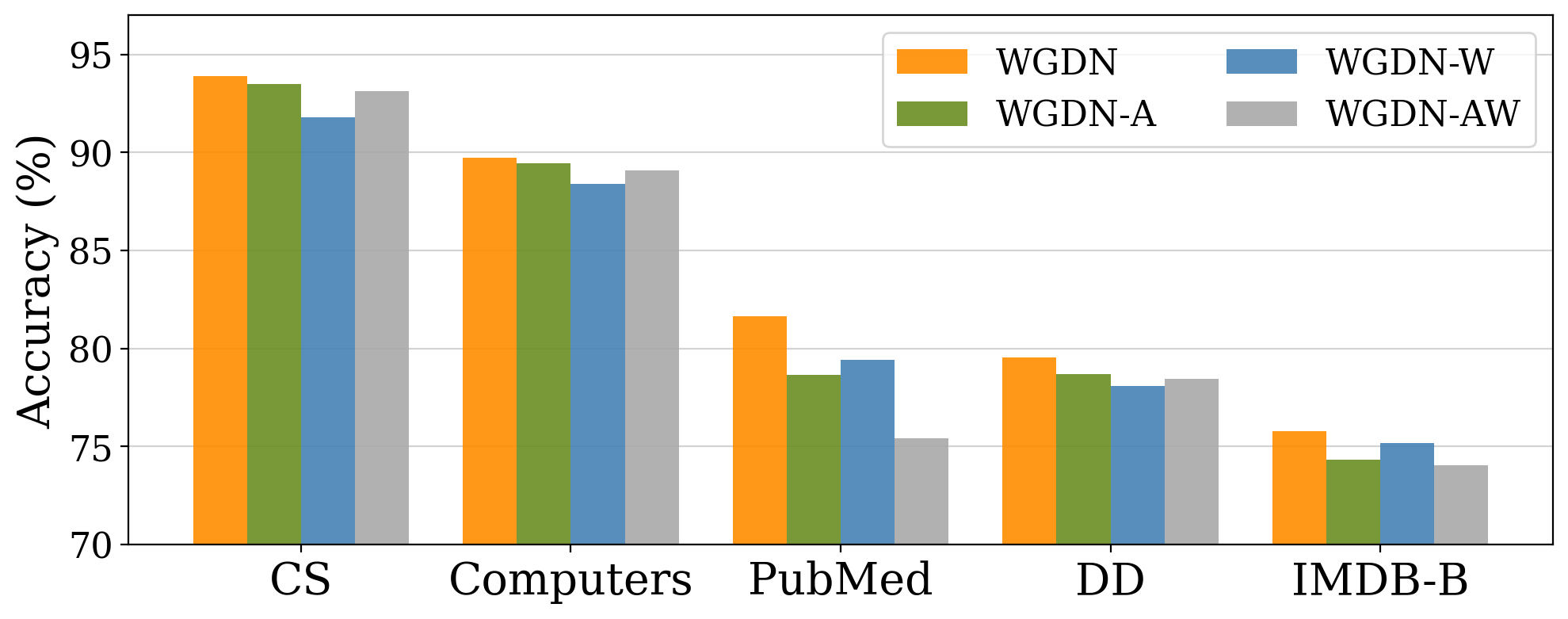
Figure 3: Ablation study of graph wiener decoder. Complete model consistently boosts model performance across different datasets.

Dataset	Model	Steps/Second	Memory
Computers	BGRL	17.27	3.01 GB
	GraphMAE	19.47	2.03 GB
	WGDN	19.62	2.20 GB
OGBN-Arxiv	BGRL	2.52	9.74 GB
	GraphMAE	3.13	8.01 GB
	WGDN	3.16	7.35 GB

Table 4: Comparison of computational efficiency on benchmark datasets.

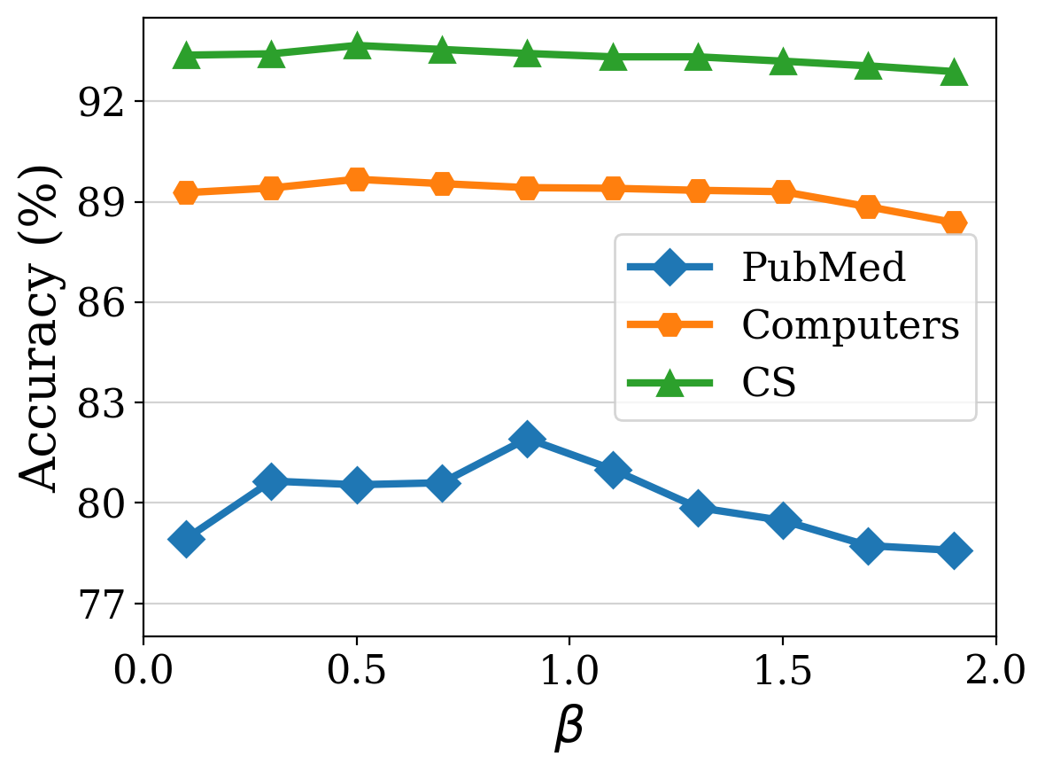
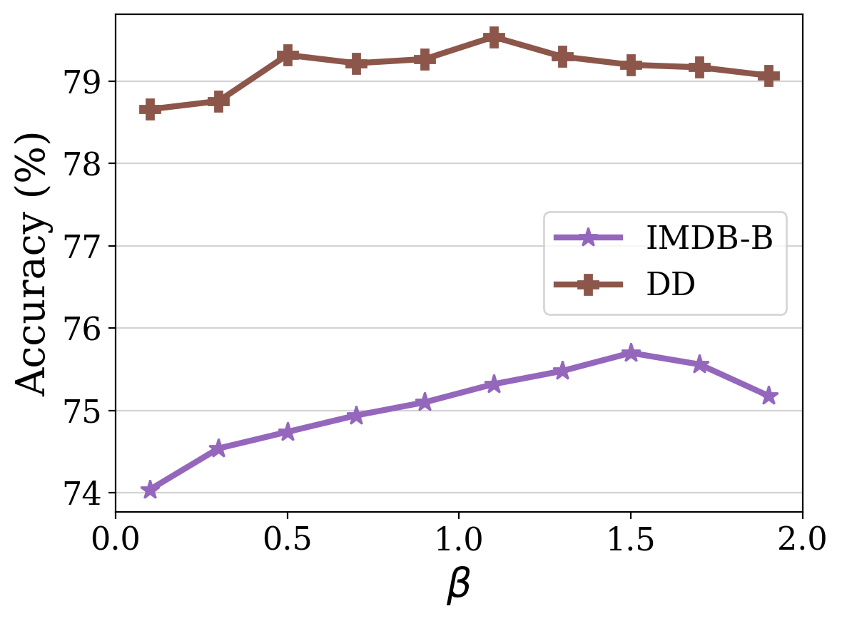
Figure 4: Downstream tasks performance versus varied augmentation magnitude $\beta$ in training.

Filter	GCN	Heat	PPR
PubMed	80.2 (0.019)	81.9 (0.011)	81.4 (0.013)
Computers	89.03 (0.417)	89.72 (0.375)	89.59 (0.405)
CS	92.48 (0.263)	93.67 (0.241)	92.75 (0.245)
IMDB-B	75.46 (0.102)	75.71 (0.098)	75.76 (0.093)
DD	79.29 (0.118)	79.36 (0.104)	79.54 (0.074)

Table 5: Performance and training loss of WGDN with different convolution filter $g_{c}$.

5.5 Hyper-parameter analysis (Q4)

Magnitude of Augmentation $\beta$.

It is expected that introducing adequate augmentation enriches the sample distribution in the latent space, which contributes to learning more expressive representations. Figure 4 shows that the classification accuracy generally reaches the peak and drops gradually when the augmentation size $\beta$ increases, which aligns with our intuition. We also observe that the optimal augmentation magnitudes are relatively smaller for node-level datasets, which may be related to the semantics level of graph features. Input features of graph-level datasets are less informative and latent distribution may still preserve with stronger augmentations. Besides, the stable trend further verifies that graph wiener decoder is well adapted to augmentation in representation learning.

Convolution filter $g_{c}$.

Table 5 shows the influence of different convolution filters. It is observed that diffusion-based WGDN outperforms its trivial version with GCN filter across different applications. Specifically, heat kernel generates better results in node classification and PPR kernel is more suitable for graph-level tasks. We conjecture that sparse feature information may be better compressed via propagation with PPR kernel. In addition, we also find that training loss of diffusion models is consistently lower. Both phenomena indicate that the superior information aggregation and powerful reconstruction of diffusion filters jointly contribute to learning a more semantic representation.

6 Conclusion and future work

In this paper, we propose Wiener Graph Deconvolutional Network (WGDN), a predictive self-supervised learning framework for graph-structured data. We introduce graph wiener filter and theoretically validate its superior reconstruction ability to facilitate reconstruction-based representation learning. By leveraging graph wiener decoder, our model can efficiently learn graph embedding with augmentation. Extensive experimental results on various datasets demonstrate that WGDN achieves competitive performance over a wide range of self-supervised and semi-supervised counterparts.

Technical Appendix

In the technical appendix, we provide further details for the proofs, model architectures and experiment.

Appendix A Proof of Proposition 4.1

Proof.

By substitution, $\mathbf{\hat{x}}_{inv}=\mathbf{x}+\mathbf{U}g_{d}(\mathbf{\Lambda})\mathbf{U}^{T}\mathbf{\epsilon}$. Note that MSE is reduced to

$$\mathbb{E}\norm{\mathbf{x}-\mathbf{\hat{x}}_{inv}}_{2}^{2}=\mathbb{E}\norm{\mathbf{U}g_{d}(\mathbf{\Lambda})\mathbf{U}^{T}\mathbf{\epsilon}}_{2}^{2}=\sum_{i=1}^{N}\frac{\sigma^{2}}{g_{c}^{2}(\lambda_{i})}.$$ (16)

Regarding the condition $g_{c}:[0,2]\mapsto[-1,1]$, we take GCN where $g_{c}(\lambda_{i})=1-\lambda_{i}$ as a representative example. By substitution, we have

$$\mathbb{E}\norm{\mathbf{x}-\mathbf{\hat{x}}_{inv}}_{2}^{2}=\sum_{i=1}^{N}\frac{\sigma^{2}}{(1-\lambda_{i})^{2}},$$ (17)

and $\frac{1}{(1-\lambda_{i})^{2}}\to\infty$ when $\lambda_{i}\to 1$. ∎

Appendix B Proof of Proposition 4.2

Proof.

By the definition of $g_{w}(\lambda_{i})$

$$\mathbb{E}\norm{\mathbf{x}-\mathbf{\hat{x}}_{w}}_{2}^{2} =\sum_{i=1}^{N}\frac{\sigma^{2}(g_{c}^{2}(\lambda_{i})+\sigma^{2}/\mathbb{E}[x^{\ast 2}_{i}])}{(g_{c}^{2}(\lambda_{i})+\sigma^{2}/\mathbb{E}[x^{\ast 2}_{i}])^{2}}$$ (18)

$$=\sum_{i=1}^{N}\frac{\sigma^{2}}{g_{c}^{2}(\lambda_{i})+\sigma^{2}/\mathbb{E}[x^{\ast 2}_{i}]}$$

$$\leq\sum_{i=1}^{N}\frac{\sigma^{2}}{g_{c}^{2}(\lambda_{i})}.$$

Plugging in the inverse filter, we can obtain

$$\sum_{i=1}^{N}\mathbb{VAR}[\mathbf{\hat{x}}_{inv,i}]$$ (19)

$$=\text{Tr}(\mathbb{COV}[\mathbf{\hat{x}}_{inv}])$$

$$=\text{Tr}(\mathbb{COV}[\mathbf{U}\mathbf{x}^{\ast}]+\mathbb{COV}[\mathbf{U}g_{d}(\mathbf{\Lambda})\mathbf{\epsilon}^{\ast}])$$

$$=\sum_{i=1}^{N}(\mathbb{VAR}[\mathbf{x}^{\ast}_{i}]+\frac{\sigma^{2}}{g_{c}^{2}(\lambda_{i})}),$$

where Tr represents the matrix trace. Similarly, variance of $\mathbf{\hat{x}}_{w}$ is convoluted by $g_{w}(\lambda_{i})$

$$\sum_{i=1}^{N}\mathbb{VAR}[\mathbf{\hat{x}}_{w,i}]$$ (20)

$$=\text{Tr}(\mathbb{COV}[\mathbf{\hat{x}}_{w}])$$

$$=\sum_{i=1}^{N}[\frac{g_{c}^{2}(\lambda_{i})}{g_{c}^{2}(\lambda_{i})+\sigma^{2}/\mathbb{E}[x^{\ast 2}_{i}]}]^{2}(\mathbb{VAR}[\mathbf{x}^{\ast}_{i}]+\frac{\sigma^{2}}{g_{c}^{2}(\lambda_{i})})$$

$$\leq\sum_{i=1}^{N}(\mathbb{VAR}[\mathbf{x}^{\ast}_{i}]+\frac{\sigma^{2}}{g_{c}^{2}(\lambda_{i})}).$$

∎

Appendix C Proof of Proposition 4.3

Proof.

Similar to Appendix B, variance of $\mathbf{\hat{x}}_{w,\gamma}$ is reduced to

$$\sum_{i=1}^{N}\mathbb{VAR}(\mathbf{\hat{x}}_{w,\gamma,i})$$ (21)

$$=\text{Tr}(\mathbb{COV}(\mathbf{\hat{x}}_{w,\gamma}))$$

$$=\sum_{i=1}^{N}[\frac{g_{c}^{2}(\lambda_{i})}{g_{c}^{2}(\lambda_{i})+\sigma^{2}/x^{\ast 2}_{\gamma}}]^{2}(\mathbb{VAR}[\mathbf{x}^{\ast}_{i}]+\frac{\sigma^{2}}{g_{c}^{2}(\lambda_{i})})$$

$$\leq\sum_{i=1}^{N}(\mathbb{VAR}[\mathbf{x}^{\ast}_{i}]+\frac{\sigma^{2}}{g_{c}^{2}(\lambda_{i})}).$$

For the specific spectrum $\lambda_{i}$ where $\mathbb{E}[x^{\ast 2}_{i}]\leq\bar{x}^{\ast 2}_{\gamma}$ holds, the spectral reconstruction error satisfies

$$S(\lambda_{i},x^{\ast}_{i},\sigma,g_{c},\bar{g}_{w,\gamma})$$ (22)

$$=\frac{1}{(g_{c}^{2}(\lambda_{i})+\sigma^{2}/\bar{x}^{\ast 2}_{\gamma})^{2}}[\sigma^{2}(g_{c}^{2}(\lambda_{i})+\frac{\sigma^{2}}{\bar{x}^{\ast 2}_{\gamma}}\cdot\frac{\mathbb{E}[x^{\ast 2}_{i}]}{\bar{x}^{\ast 2}_{\gamma}})]$$

$$\leq\frac{1}{(g_{c}^{2}(\lambda_{i})+\sigma^{2}/\bar{x}^{\ast 2}_{\gamma})^{2}}[\sigma^{2}(g_{c}^{2}(\lambda_{i})+\frac{\sigma^{2}}{\bar{x}^{\ast 2}_{\gamma}})]$$

$$=\frac{\sigma^{2}}{g_{c}^{2}(\lambda_{i})+\sigma^{2}/\bar{x}^{\ast 2}_{\gamma}}$$

$$\leq\frac{\sigma^{2}}{g_{c}^{2}(\lambda_{i})}=S(\lambda_{i},x^{\ast}_{i},\sigma,g_{c},g_{c}^{-1}).$$

Note that the second derivative of spectral reconstruction error $S(\lambda_{i},x^{\ast}_{i},\sigma,g_{c},g_{d})$ with respect to $g_{d}(\lambda_{i})$ is

$$\frac{\partial^{2}}{\partial g_{d}^{2}(\lambda_{i})}S(\lambda_{i},x^{\ast}_{i},\sigma,g_{c},g_{d})$$ (23)

$$=2(g_{c}^{2}(\lambda_{i})\mathbb{E}[x^{\ast 2}_{i}]+\sigma^{2})\geq 0,$$

thus, $S(\lambda_{i},x^{\ast}_{i},\sigma,g_{c},g_{d})$ is a convex function. By Eq. 6, $g_{w}(\lambda_{i})$ is the solution for global minimum. By convexity, for any filter $g_{d}(\lambda_{i})$, the value of $S(\lambda_{i},x^{\ast}_{i},\sigma,g_{c},g_{d})$ is greater when distance to global minimizer $|g_{d}(\lambda_{i})-g_{w}(\lambda_{i})|$ is larger. Considering $\bar{g}_{w,\gamma}(\lambda_{i})$, it can be reduced to

$$|\bar{g}_{w,\gamma}(\lambda_{i})-g_{w}(\lambda_{i})|$$ (24)

$$=|\frac{g_{c}(\lambda_{i})}{g_{c}^{2}(\lambda_{i})+\sigma^{2}/\bar{x}^{\ast 2}_{\gamma}}-\frac{g_{c}(\lambda_{i})}{g_{c}^{2}(\lambda_{i})+\sigma^{2}/\mathbb{E}[x^{\ast 2}_{i}]}|.$$

Given the condition that $x^{\ast 2}_{i}\leq\bar{x}^{\ast 2}_{\gamma_{1}}\leq\bar{x}^{\ast 2}_{\gamma_{2}}$, we can conclude that

$$|\bar{g}_{w,\gamma_{1}}(\lambda_{i})-g_{w}(\lambda_{i})|\leq|\bar{g}_{w,\gamma_{2}}(\lambda_{i})-g_{w}(\lambda_{i})|.$$ (25)

Therefore, $S(\lambda_{i},x^{\ast}_{i},\sigma,g_{c},\bar{g}_{w,\gamma_{1}})\leq S(\lambda_{i},x^{\ast}_{i},\sigma,g_{c},\bar{g}_{w,\gamma_{2}})\leq S(\lambda_{i},x^{\ast}_{i},\sigma,g_{c},g_{c}^{-1})$ holds. ∎

Model	PubMed	Computers	Photo	CS	Physics
BGRL${}_{\text{N}}$	78.6 $\pm$ 0.7	89.49 $\pm$ 0.21	93.01 $\pm$ 0.20	93.15 $\pm$ 0.12	95.14 $\pm$ 0.06
BGRL${}_{\text{H}}$	79.8 $\pm$ 0.4	89.70 $\pm$ 0.15	93.37 $\pm$ 0.21	93.51 $\pm$ 0.10	95.24 $\pm$ 0.09
BGRL${}_{\text{P}}$	79.4 $\pm$ 0.5	89.63 $\pm$ 0.17	93.15 $\pm$ 0.21	93.42 $\pm$ 0.12	95.28 $\pm$ 0.06
AFGRL${}_{\text{N}}$	79.5 $\pm$ 0.2	88.91 $\pm$ 0.37	92.96 $\pm$ 0.25	93.17 $\pm$ 0.15	95.54 $\pm$ 0.09
AFGRL${}_{\text{H}}$	79.9 $\pm$ 0.3	89.58 $\pm$ 0.45	93.61 $\pm$ 0.20	93.56 $\pm$ 0.15	95.74 $\pm$ 0.10
AFGRL${}_{\text{P}}$	79.7 $\pm$ 0.3	89.33 $\pm$ 0.37	93.06 $\pm$ 0.27	93.53 $\pm$ 0.14	95.71 $\pm$ 0.10
CCA-SSG${}_{\text{N}}$	80.5 $\pm$ 0.3	87.35 $\pm$ 0.30	92.38 $\pm$ 0.33	93.31 $\pm$ 0.16	95.14 $\pm$ 0.07
CCA-SSG${}_{\text{H}}$	81.0 $\pm$ 0.3	88.15 $\pm$ 0.35	93.25 $\pm$ 0.25	-	95.59 $\pm$ 0.07
CCA-SSG${}_{\text{P}}$	80.7 $\pm$ 0.3	87.27 $\pm$ 0.46	92.79 $\pm$ 0.25	-	95.12 $\pm$ 0.13
$\text{WGDN}_{\text{N}}$	80.2 $\pm$ 0.4	89.03 $\pm$ 0.46	92.26 $\pm$ 0.37	92.48 $\pm$ 0.12	95.33 $\pm$ 0.02
$\text{WGDN}_{\text{H}}$	81.9 $\pm$ 0.4	89.72 $\pm$ 0.48	93.89 $\pm$ 0.31	93.67 $\pm$ 0.17	95.76 $\pm$ 0.11
$\text{WGDN}_{\text{P}}$	81.4 $\pm$ 0.3	89.59 $\pm$ 0.45	92.96 $\pm$ 0.19	92.75 $\pm$ 0.21	95.40 $\pm$ 0.23

Table 6: Node classification accuracy with different encoding propagation backbones.

Model	PubMed	Comp	CS	IMDB-B	DD
AFGRL	79.9 $\pm$ 0.3	89.58 $\pm$ 0.45	93.56 $\pm$ 0.15	75.07 $\pm$ 0.58	78.58 $\pm$ 0.44
GraphMAE	81.1 $\pm$ 0.4	89.53 $\pm$ 0.31	93.51 $\pm$ 0.13	75.52 $\pm$ 0.66	78.86 $\pm$ 0.35
WGDN-DE	80.9 $\pm$ 0.6	89.55 $\pm$ 0.36	93.56 $\pm$ 0.31	75.42 $\pm$ 0.15	79.24 $\pm$ 0.40
WGDN-DN	81.3 $\pm$ 0.5	89.49 $\pm$ 0.34	93.53 $\pm$ 0.31	75.52 $\pm$ 0.17	79.31 $\pm$ 0.32
WGDN	81.9 $\pm$ 0.4	89.72 $\pm$ 0.48	93.89 $\pm$ 0.31	75.76 $\pm$ 0.20	79.54 $\pm$ 0.51

Table 7: Performance of WGDN against different augmentation methods.

Appendix D Details of Model Architecture

AER estimation.

Let $\mathbf{\hat{H}}^{(m)}$ denotes the input of $m$-th layer decoder, the average spectral energy $\bar{x}^{\ast 2}_{\gamma_{i}}$ in $\mathbf{D}_{\gamma_{i}}^{(m)}$ is estimated following $\sum_{i=1}^{N}\mathbb{E}[x^{\ast 2}_{i}]=\sum_{i=1}^{N}\mathbb{E}[x^{2}_{i}]=\sum_{i=1}^{N}{\mathbb{E}[x_{i}]}^{2}+\mathbb{VAR}[x_{i}]$. Specifically,

$$\bar{x}^{\ast 2}_{\gamma_{i}}=\frac{\gamma_{i}}{ND^{\prime}}\big{(}\norm{\mathbf{\hat{H}}^{(m)}}_{F}^{2}+\norm{\mathbf{\hat{H}}^{(m)}-\frac{1}{N}\mathds{1}\mathbf{\hat{H}}^{(m)}}_{F}^{2}\big{)},$$ (26)

where $\mathds{1}\in\mathbb{R}^{N\times D^{\prime}}$ is the all ones matrix and $D^{\prime}$ is the size of hidden space. The augmentation variance $\sigma^{2}$ is estimated by considering its neighborhood as

$$\sigma^{2}=\frac{1}{ND^{\prime}}\norm{\mathbf{\hat{H}}^{(m)}-\mathbf{D}^{-1}\mathbf{A}\mathbf{\hat{H}}^{(m)}}_{F}^{2},$$ (27)

where $\mathbf{A}$ and $\mathbf{D}$ are adjacency matrix and degree matrix.

Skip connection.

To learn more expressive representations, skip connection is considered in training phase for some cases as it transmits aggregated information to create ’hard’ examples for decoder, which may encourage encoder to compress more useful knowledge. If skip connection is implemented, we let $\mathbf{\hat{H}}^{(m)}_{d}=\mathbf{\hat{H}}^{(m)}$ for clarity. For $m=1,..,M-1$, we augment the output of the $m$-layer encoder, denoted as $\mathbf{\hat{H}}^{(m)}_{e}$, by

$$\mathbf{\hat{H}}^{(m)}_{e}=\mathbf{H}^{(m)}+\beta\mathbf{E}^{(m)},$$ (28)

where $\mathbf{E}^{(m)}=\{\mathbf{\epsilon}_{1}^{(m)},...,\mathbf{\epsilon}_{N}^{(m)}\}$, $\mathbf{\epsilon}_{i}^{(m)}\sim N(\mathbf{0},\sigma_{P}^{2\,(m)}\mathbf{I})$, $\sigma_{P}^{2\,(m)}=\mathbb{VAR}[\mathbf{H}^{(m)}]$ and $\beta$ is same hyper-parameter in Eq. 13. To avoid learning trivial representation, both augmented representations are fed into the same decoder as

$$\mathbf{Z}^{(m-1)}_{i,s} =\phi(\mathbf{D}_{\gamma_{i},s}^{(m)}\mathbf{\hat{H}}^{(m)}_{s}\mathbf{W}^{(m)}_{i}),$$ (29)

$$\mathbf{\hat{H}}^{(m-1)}_{s} =\text{AGG}([\mathbf{Z}^{(m-1)}_{1,s},...,\mathbf{Z}^{(m-1)}_{q,s}]),$$

where $s=\{e,d\}$ represents the source. The final representation of $m$-layer decoder is obtained by averaging the intermediate embeddings,

$$\mathbf{\hat{H}}^{(m-1)}=\text{AVG}(\mathbf{\hat{H}}^{(m-1)}_{e},\mathbf{\hat{H}}^{(m-1)}_{d}).$$ (30)

Normalization.

For graph classification, we apply batch normalization (Ioffe and Szegedy 2015) right before activation function for all layers except the final prediction layer.

Appendix E More Experimental Results

E.1 Experiment on Encoder Backbones

To have a fair comparison with contrastive methods, we compare WGDN with the three state-of-the-art baselines using spectral kernel in node classification task. For clarity, models with GCN, heat and PPR kernel are denoted with subscript ${}_{\text{N}}$, ${}_{\text{H}}$ and ${}_{\text{P}}$ respectively.

From Table 6, it is observed that WGDN still achieves better performance over baselines trained with spectral kernels. In terms of CS, CCA-SSG employs MLP as its decoder because GNN decoders worsen model performance under its experiment settings. In addition, utilizing spectral propagation consistently boosts the learning capability, which aligns with our motivation pertaining to the potential of graph spectral kernel. Particularly, for node classification, heat kernel may be a better option, as it brings the greatest improvement regardless of datasets and model types.

Dataset	Cora	CiteSeer	PubMed	Computers	Photo	CS	Physics	OGBN-Arxiv
# Nodes	2,708	3,327	19,717	13,752	7,650	18,333	34,493	169,343
# Edges	10,556	9,104	88,648	491,722	238,162	163,788	495,924	1,166,243
# Classes	7	6	3	10	8	15	5	40
# Features	1,433	3,703	500	767	745	8,415	8,415	128
Augmentation $\beta$	0.9	1.0	1.0	0.4	0.5	0.5	0.2	0.8
Hidden Size	512	512	1024	512	512	512	512	768
Epoch	100	100	300	1000	1000	150	100	120
Filter $g_{c}(\lambda_{i})$	PPR	PPR	Heat	Heat	Heat	Heat	Heat	PPR
Aggregation	Max	Sum	Max	-	-	-	-	-
Last Activation	✓	-	-	✓	-	-	✓	-
Skip Connection	✓	-	✓	-	-	✓	✓	-

Table 8: Summary of datasets and hyper-parameter configuration for node classification task.

Dataset	IMDB-B	IMDB-M	PROTEINS	COLLAB	DD	NCI1
# Graphs	1,000	1,500	1,113	5,000	1,178	4,110
# Avg. Nodes	19.77	13.00	39.06	74.49	284.32	29.87
# Avg. Edges	193.06	65.94	72.82	2457.78	715.66	32.30
# Classes	2	3	2	3	2	2
Augmentation $\beta$	1.5	1.5	1.0	1.0	1.0	0.5
Learning Rate	0.0001	0.0001	0.0001	0.0001	0.0001	0.0005
Batch Size	32	32	32	32	32	16
Epoch	100	100	10	20	40	500
Filter $g_{c}(\lambda_{i})$	PPR	PPR	PPR	PPR	PPR	Heat
Aggregation	Max	Avg	Avg	-	Avg	-
Pooling	Avg	Avg	Max	Max	Sum	Max
Skip Connection	✓	✓	✓	✓	✓	-

Table 9: Summary of datasets and hyper-parameter configuration for graph classification task.

E.2 Experiment on Different Augmentations

Although the graph wiener decoder is derived based on latent augmentations, a powerful decoder should adapt to general augmentation techniques. We conduct experiments with five representative datasets with drop-edge and drop-node, which are denoted as WGDN-DE and WGDN-DN respectively. Table 7 shows that different variants of our framework still achieve comparable performance with competitive baselines on both node and graph classification. However, general augmentations hardly satisfy the distribution assumption, resulting in inaccurate noise estimation and performance degradation.

E.3 Experiments on Additional Datasets

To evaluate the effectiveness of our proposed method, three more commonly used datasets are considered. For fair comparisons, we conducted hyper-parameter search to finetune the most competitive baselines. We report the results in Table 10 and find that WGDN still achieves state-of-the-art performances in 2 out of 3 datasets.

Model	Cora	CiteSeer	OBGN-Arxiv
BGRL	82.8 $\pm$ 0.5	71.3 $\pm$ 0.8	71.64 $\pm$ 0.12
AFGRL	81.7 $\pm$ 0.4	71.2 $\pm$ 0.4	71.39 $\pm$ 0.16
CCA-SSG	83.8 $\pm$ 0.5	73.1 $\pm$ 0.3	71.24 $\pm$ 0.20
WGDN	84.2 $\pm$ 0.6	72.2 $\pm$ 1.1	71.76 $\pm$ 0.23

Table 10: Node classification accuracy on additional commonly used datasets.

Appendix F Detailed Experimental Setup

F.1 Evaluation Protocol

For node classification tasks, all the resulted embedding from well-trained unsupervised models are frozen. We use Glorot initialization (Glorot and Bengio 2010) to initialize model parameters and all downstream models are trained for 300 epochs by Adam optimizer (Kingma and Ba 2015) with a learning rate 0.01. We run 20 trials and keep the model with the highest performance in validation set of each run as final. For graph classification tasks, linear SVM is fine-tuned with grid search on C parameter from $\{10^{-3},10^{-2},...,1,10\}$.

F.2 Hyper-parameter Specifications

By default, wiener graph decoder is implemented with multiple channels with $q=3$ and $\gamma=[0.1,1,10]$. Otherwise, single channel is used with $\gamma=1$. Aggregation function is applied only in the scenarios of multiple channels. For wiener kernel approximation, the polynomial order $K$ of GCN kernel is 9 while others are 2. All models are initialized using Glorot initialization (Glorot and Bengio 2010) and optimized by Adam optimizer (Kingma and Ba 2015).

For node classification, we set the learning rate as 0.001. The number of layers is 3 for OGBN-Arxiv and set as 2 for the remaining datasets. To enhance the representation power of embedding, no activation function is employed in the last layer of encoder in some cases. For graph classification, the dimension of hidden embedding is set to 512. The number of layer is set to 3 for IMDB-M as well as PROTEINS and 2 for the rest. The detailed hyper-parameter configurations of each dataset are illustrated in Table 8 and 9.

F.3 Baselines Implementations

For node classification, we use the official implementation of BGRL, AFGRL and CCA-SSG and follow the suggested hyper-parameter settings for reproduction. For fair comparison in the scenarios of spectral kernel implementation, we conduct hyper-parameter search for them and select the model with best results in validation set as final.

For graph classification, we report the previous results in the public papers. For dataset DD, we generate the result of GraphMAE with its source code and hyper-parameter searching.

F.4 Computational Hardware

We use the machine with the following configurations for all model training and evaluation.

• OS: Ubuntu 20.04.1 LTS

• CPU: Intel(R) Xeon(R) Silver 4114 CPU @ 2.20GHz

• GPU: NVIDIA Tesla V100, 32GB

References

- Balcilar et al. (2021) Balcilar, M.; Renton, G.; Héroux, P.; Gaüzère, B.; Adam, S.; and Honeine, P. 2021. Analyzing the expressive power of graph neural networks in a spectral perspective. In ICLR.
- Burden, Faires, and Burden (2015) Burden, R. L.; Faires, J. D.; and Burden, A. M. 2015. Numerical analysis. Cengage learning.
- Cheung and Yeung (2021) Cheung, T.-H.; and Yeung, D.-Y. 2021. MODALS: Modality-agnostic Automated Data Augmentation in the Latent Space. In ICLR.
- Devlin et al. (2019) Devlin, J.; Chang, M.-W.; Lee, K.; and Toutanova, K. 2019. Bert: Pre-training of deep bidirectional transformers for language understanding. In NAACL.
- Dong, Roth, and Schiele (2020) Dong, J.; Roth, S.; and Schiele, B. 2020. Deep Wiener Deconvolution: Wiener Meets Deep Learning for Image Deblurring. In NeurIPS.
- Gasteiger, Bojchevski, and Günnemann (2019) Gasteiger, J.; Bojchevski, A.; and Günnemann, S. 2019. Combining Neural Networks with Personalized PageRank for Classification on Graphs. In ICLR.
- Glorot and Bengio (2010) Glorot, X.; and Bengio, Y. 2010. Understanding the difficulty of training deep feedforward neural networks. In AISTATS.
- Grill et al. (2020) Grill, J.-B.; Strub, F.; Altché, F.; Tallec, C.; Richemond, P.; Buchatskaya, E.; Doersch, C.; Avila Pires, B.; Guo, Z.; Gheshlaghi Azar, M.; et al. 2020. Bootstrap your own latent-a new approach to self-supervised learning. In NeurIPS.
- Grover and Leskovec (2016) Grover, A.; and Leskovec, J. 2016. node2vec: Scalable feature learning for networks. In KDD.
- Hassani and Khasahmadi (2020) Hassani, K.; and Khasahmadi, A. H. 2020. Contrastive multi-view representation learning on graphs. In ICML.
- He et al. (2020) He, K.; Fan, H.; Wu, Y.; Xie, S.; and Girshick, R. 2020. Momentum contrast for unsupervised visual representation learning. In CVPR.
- Hou et al. (2022) Hou, Z.; Liu, X.; Cen, Y.; Dong, Y.; Yang, H.; Wang, C.; and Tang, J. 2022. GraphMAE: Self-Supervised Masked Graph Autoencoders. In KDD.
- Hu et al. (2020a) Hu, W.; Fey, M.; Zitnik, M.; Dong, Y.; Ren, H.; Liu, B.; Catasta, M.; and Leskovec, J. 2020a. Open Graph Benchmark: Datasets for Machine Learning on Graphs. arXiv preprint arXiv:2005.00687.
- Hu et al. (2020b) Hu, W.; Liu, B.; Gomes, J.; Zitnik, M.; Liang, P.; Pande, V.; and Leskovec, J. 2020b. Strategies for pre-training graph neural networks. In ICLR.
- Ioffe and Szegedy (2015) Ioffe, S.; and Szegedy, C. 2015. Batch normalization: Accelerating deep network training by reducing internal covariate shift. In ICML.
- Jin and Zhang (2019) Jin, H.; and Zhang, X. 2019. Latent Adversarial Training of Graph Convolutional Networks. In ICML workshop on Learning and Reasoning with Graph-Structured Representations.
- Kingma and Ba (2015) Kingma, D. P.; and Ba, J. 2015. Adam: A method for stochastic optimization. In ICLR.
- Kipf and Welling (2016) Kipf, T. N.; and Welling, M. 2016. Variational Graph Auto-Encoders. In NeurIPS Workshop on Bayesian Deep Learning.
- Kipf and Welling (2017) Kipf, T. N.; and Welling, M. 2017. Semi-Supervised Classification with Graph Convolutional Networks. In ICLR.
- Klicpera, Weißenberger, and Günnemann (2019) Klicpera, J.; Weißenberger, S.; and Günnemann, S. 2019. Diffusion Improves Graph Learning. In NeurIPS.
- Lee, Lee, and Park (2022) Lee, N.; Lee, J.; and Park, C. 2022. Augmentation-free self-supervised learning on graphs. In AAAI.
- Li et al. (2021) Li, J.; Li, J.; Liu, Y.; Yu, J.; Li, Y.; and Cheng, H. 2021. Deconvolutional Networks on Graph Data. In NeurIPS, volume 34, 21019–21030.
- Li et al. (2020a) Li, J.; Yu, J.; Li, J.; Zhang, H.; Zhao, K.; Rong, Y.; Cheng, H.; and Huang, J. 2020a. Dirichlet graph variational autoencoder. Advances in Neural Information Processing Systems, 33: 5274–5283.
- Li et al. (2020b) Li, J.; Yu, T.; Juan, D.-C.; Gopalan, A.; Cheng, H.; and Tomkins, A. 2020b. Graph Autoencoders with Deconvolutional Networks. arXiv preprint arXiv:2012.11898.
- Liu et al. (2022) Liu, Y.; Pan, S.; Jin, M.; Zhou, C.; Xia, F.; and Yu, P. S. 2022. Graph self-supervised learning: A survey. IEEE Transactions on Knowledge and Data Engineering.
- Morris et al. (2020) Morris, C.; Kriege, N. M.; Bause, F.; Kersting, K.; Mutzel, P.; and Neumann, M. 2020. TUDataset: A collection of benchmark datasets for learning with graphs. In ICML Workshop on Graph Representation Learning and Beyond.
- Narayanan et al. (2017) Narayanan, A.; Chandramohan, M.; Venkatesan, R.; Chen, L.; Liu, Y.; and Jaiswal, S. 2017. graph2vec: Learning distributed representations of graphs. arXiv preprint arXiv:1707.05005.
- Pachon and Trefethen (2009) Pachon, R.; and Trefethen, L. 2009. Barycentric-Remez algorithms for best polynomial approximation in the chebfun system. BIT.
- Pan et al. (2018) Pan, S.; Hu, R.; Long, G.; Jiang, J.; Yao, L.; and Zhang, C. 2018. Adversarially regularized graph autoencoder for graph embedding. In IJCAI.
- Park et al. (2019) Park, J.; Lee, M.; Chang, H. J.; Lee, K.; and Choi, J. Y. 2019. Symmetric Graph Convolutional Autoencoder for Unsupervised Graph Representation Learning. In ICCV.
- Perozzi, Al-Rfou, and Skiena (2014) Perozzi, B.; Al-Rfou, R.; and Skiena, S. 2014. Deepwalk: Online learning of social representations. In KDD.
- Perraudin and Vandergheynst (2017) Perraudin, N.; and Vandergheynst, P. 2017. Stationary Signal Processing on Graphs. IEEE Transactions on Signal Processing.
- Salehi and Davulcu (2020) Salehi, A.; and Davulcu, H. 2020. Graph Attention Auto-Encoders. In ICTAI.
- Sen et al. (2008) Sen, P.; Namata, G.; Bilgic, M.; Getoor, L.; Galligher, B.; and Eliassi-Rad, T. 2008. Collective classification in network data. AI magazine.
- Shchur et al. (2018) Shchur, O.; Mumme, M.; Bojchevski, A.; and Günnemann, S. 2018. Pitfalls of Graph Neural Network Evaluation. In NeurIPS Workshop on Relational Representation Learning.
- Shervashidze et al. (2011) Shervashidze, N.; Schweitzer, P.; Van Leeuwen, E. J.; Mehlhorn, K.; and Borgwardt, K. M. 2011. Weisfeiler-lehman graph kernels. JMLR.
- Son and Lee (2017) Son, H.; and Lee, S. 2017. Fast non-blind deconvolution via regularized residual networks with long/short skip-connections. In ICCP.
- Sun et al. (2019) Sun, F.-Y.; Hoffman, J.; Verma, V.; and Tang, J. 2019. InfoGraph: Unsupervised and Semi-supervised Graph-Level Representation Learning via Mutual Information Maximization. In ICLR.
- Thakoor et al. (2022) Thakoor, S.; Tallec, C.; Azar, M. G.; Azabou, M.; Dyer, E. L.; Munos, R.; Veličković, P.; and Valko, M. 2022. Large-Scale Representation Learning on Graphs via Bootstrapping. In ICLR.
- Veličković et al. (2018) Veličković, P.; Cucurull, G.; Casanova, A.; Romero, A.; Liò, P.; and Bengio, Y. 2018. Graph Attention Networks. In ICLR.
- Veličković et al. (2019) Veličković, P.; Fedus, W.; Hamilton, W. L.; Liò, P.; Bengio, Y.; and Hjelm, R. D. 2019. Deep graph infomax. In ICLR.
- Wang et al. (2017) Wang, C.; Pan, S.; Long, G.; Zhu, X.; and Jiang, J. 2017. Mgae: Marginalized graph autoencoder for graph clustering. In CIKM.
- Wiener (1964) Wiener, N. 1964. Extrapolation, Interpolation, and Smoothing of Stationary Time Series. The MIT Press.
- Wu et al. (2019) Wu, F.; Souza, A.; Zhang, T.; Fifty, C.; Yu, T.; and Weinberger, K. 2019. Simplifying Graph Convolutional Networks. In ICML.
- Xia et al. (2022) Xia, J.; Wu, L.; Chen, J.; Hu, B.; and Li, S. Z. 2022. SimGRACE: A Simple Framework for Graph Contrastive Learning without Data Augmentation. In WWW.
- Xie et al. (2022) Xie, Y.; Xu, Z.; Zhang, J.; Wang, Z.; and Ji, S. 2022. Self-supervised learning of graph neural networks: A unified review. IEEE Transactions on Pattern Analysis and Machine Intelligence.
- Xu et al. (2021) Xu, D.; Cheng, W.; Luo, D.; Chen, H.; and Zhang, X. 2021. Infogcl: Information-aware graph contrastive learning. In NeurIPS.
- Xu et al. (2019) Xu, K.; Hu, W.; Leskovec, J.; and Jegelka, S. 2019. How Powerful are Graph Neural Networks? In ICLR.
- Yanardag and Vishwanathan (2015) Yanardag, P.; and Vishwanathan, S. 2015. Deep graph kernels. In KDD.
- Yang and Segarra (2018) Yang, J.; and Segarra, S. 2018. Enhancing geometric deep learning via graph filter deconvolution. In GlobalSIP.
- You et al. (2021) You, Y.; Chen, T.; Shen, Y.; and Wang, Z. 2021. Graph contrastive learning automated. In ICML.
- You et al. (2020a) You, Y.; Chen, T.; Sui, Y.; Chen, T.; Wang, Z.; and Shen, Y. 2020a. Graph contrastive learning with augmentations. In NeurIPS.
- You et al. (2020b) You, Y.; Chen, T.; Wang, Z.; and Shen, Y. 2020b. When does self-supervision help graph convolutional networks? In ICML.
- Zhang et al. (2020) Zhang, C.-Y.; Hu, J.; Yang, L.; Chen, C. P.; and Yao, Z. 2020. Graph deconvolutional networks. Information Sciences.
- Zhang et al. (2021) Zhang, H.; Wu, Q.; Yan, J.; Wipf, D.; and Philip, S. Y. 2021. From canonical correlation analysis to self-supervised graph neural networks. In NeurIPS.
- Zhang et al. (2022) Zhang, Y.; Zhu, H.; Song, Z.; Koniusz, P.; and King, I. 2022. COSTA: Covariance-Preserving Feature Augmentation for Graph Contrastive Learning. In KDD.
- Zhu et al. (2020) Zhu, Y.; Xu, Y.; Yu, F.; Liu, Q.; Wu, S.; and Wang, L. 2020. Deep Graph Contrastive Representation Learning. In ICML Workshop on Graph Representation Learning and Beyond.
- Zhu et al. (2021) Zhu, Y.; Xu, Y.; Yu, F.; Liu, Q.; Wu, S.; and Wang, L. 2021. Graph contrastive learning with adaptive augmentation. In WWW.