SiMa: Effective and Efficient Data Silo Federation Using Graph Neural Networks

Abstract.

Virtually every sizable organization nowadays is building a form of a data lake. In theory, every department or team in the organization would enrich their datasets with metadata, and store them in a central data lake. Those datasets can then be combined in different ways and produce added value to the organization. In practice, though, the situation is vastly different: each department has its own privacy policies, data release procedures, and goals. As a result, each department maintains its own data lake, leading to data silos. For such data silos to be of any use, they need to be integrated.

This paper presents SiMa, a method for federating data silos that consistently finds more correct relationships than the state-of-the-art matching methods, while minimizing wrong predictions and requiring 20x to 1000x less time to execute. SiMa leverages Graph Neural Networks (GNNs) to learn from the existing column relationships and automated data profiles found in data silos. Our method makes use of the trained GNN to perform link prediction and find new column relationships across data silos. Most importantly, SiMa can be trained incrementally on the column relationships within each silo individually, and does not require consolidating all datasets into one place.

1. Introduction

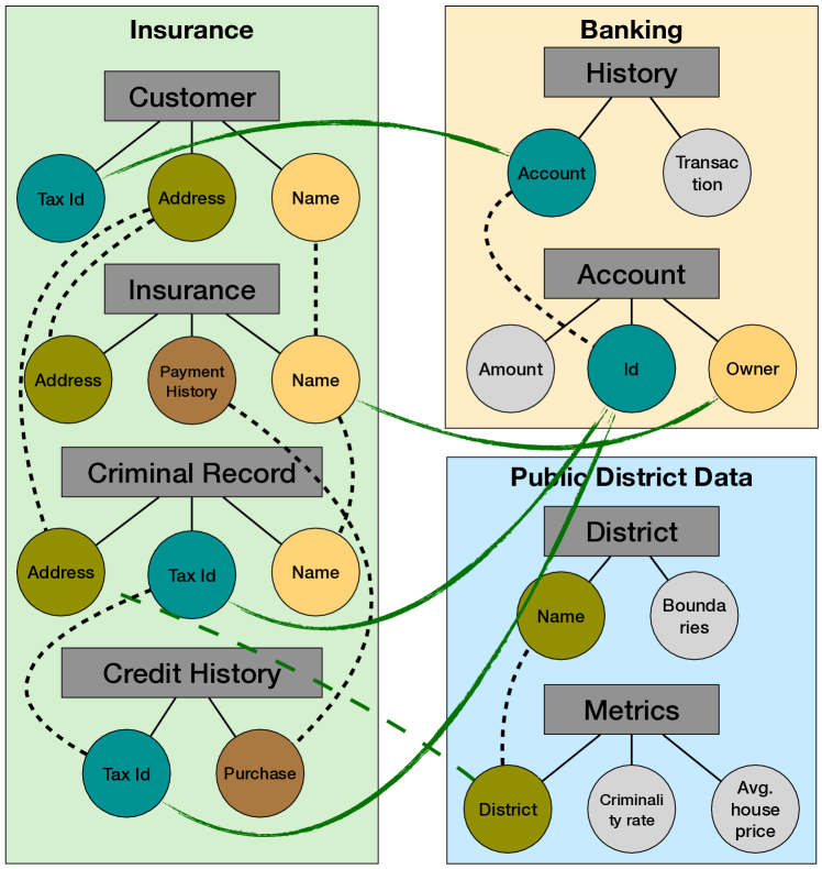
Figure 1. Three typical data silos in the banking industry.

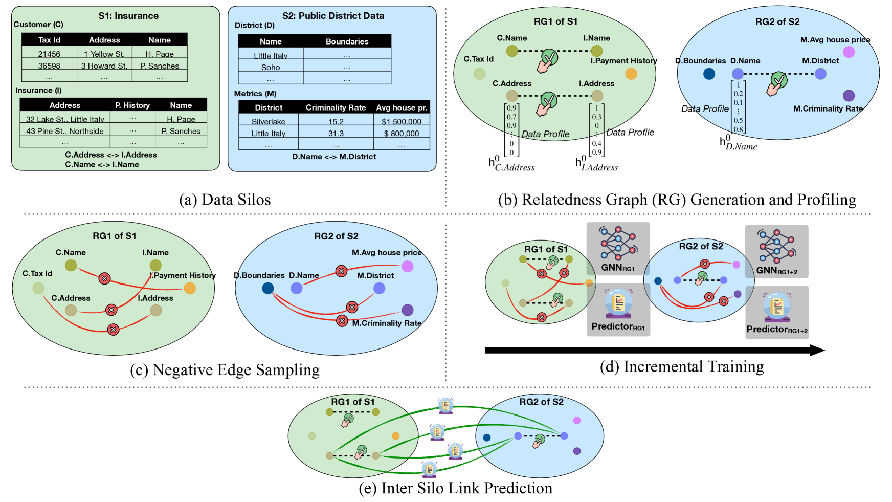
Figure 2. SiMa overview: (a) depicts data silos and their column matches which are transformed into relatedness graphs ((b)-Section 3.2), where nodes represent columns and receive their initial features from a tabular data profiler (Section 3.3). Then, negative edges are being sampled from each relatedness graph as shown in (c) (Section 4.1) and a link prediction model is being trained based on an incremental training scheme depicted in (d) (Section 4.2). Finally, using the trained model we are able to predict relationships among columns from different silos as depicted in (e).

Organizations nowadays accumulate large numbers of heterogeneous datasets in a data lake, with the goal of gaining insights across those datasets. Both the structure (e.g., departments, teams, projects) of organizations but also the regulatory context (e.g., privacy laws, contracts) force them to establish barriers for their data assets, which leads to the phenomenon of data silos: disparate collections of data, belonging to different stakeholders. Interestingly, data silos may even exist within the same organization, as individual teams enforce their own conventions and formats, as well as encapsulate knowledge about their data assets. Silo-ing data impedes collaboration and information sharing among different groups of interest. While there is knowledge about potential relationships among distinct data within a silo, there are no links across disparate silos. This means that teams working on different data silos cannot explore, neither discover valuable data connections.

Consider the example of an organization in the banking industry as depicted in Figure 1. Employees of the banking silo already know the relationships between their datasets (black dotted lines), i.e. columns from tables inside the silo that are semantically related (storing values that refer to the same semantic type). However, the possible relationships between the banking silo and the other two silos (green lines) are missing, i.e. columns of the same semantic type, residing in different silos. Data scientists building ML models can benefit from dataset augmentation in terms of extra data points (by finding other unionable datasets) and/or extra features (by finding other joinable datasets) from other data silos (Chepurko et al., 2020).

Existing solutions. Discovering relationships among columns of the same semantic type across data silos is very challenging (Mansour et al., 2021). In the data management research the problem has been investigated in the context of i) schema matching, with a multitude of automated methods either addressing it directly (Rahm and Bernstein, 2001; Zhang et al., 2011; Lehmberg and Bizer, 2017; Fernandez et al., 2018b; Koutras et al., 2020; Cappuzzo et al., 2020), or indirectly in the context of related dataset search (Fernandez et al., 2018a; Nargesian et al., 2018; Zhu et al., 2019; Bogatu et al., 2020; Zhang and Ives, 2020), and ii) column-level type classification (Hulsebos et al., 2019; Zhang et al., [n. d.]), where methods train models on large numbers of tables in order to categorize columns to a specific set of types. However, employing these methods in the setting of data silos is either infeasible, or sub-optimal.

Matching methods inapplicable to Silo Federation. Existing matching methods assume global access to all datasets so that they can compute similarities between pairs of columns. Across data silos, this is usually impossible, since the stakeholders maintaining them are not willing to share (potentially sensitive) data with each other (Miller, 2018). On the other hand, methods that base their similarity calculations on data statistics (Do and Rahm, 2002; Zhang et al., 2011) could first compute statistics of columns within a silo, and carry only those statistics over to other silos for similarity calculations. However, it is often the case that characteristics of values across silos can differ substantially, even for the same semantic types (e.g., names of people in different countries) leading to false negative matches. In addition, applying schema matching solutions (Rahm and Bernstein, 2001; Zhang et al., 2011; Lehmberg and Bizer, 2017; Fernandez et al., 2018b; Koutras et al., 2020; Cappuzzo et al., 2020) requires computation of similarities between all pairs of columns. As the number of columns $n$ increases beyond the thousands – a small number considering the size of data lakes and commercial databases – computing O($n^{2}$) similarities is impractical. In this paper we present a method that is applicable to the silo federation problem. In addition, our proposed approach is 20x to 1000x faster than existing matching methods.

Related Dataset Search methods inapplicable to Silo Federation. Related dataset search solutions make use of structures such as LSH indexes (Fernandez et al., 2018a; Nargesian et al., 2018; Bogatu et al., 2020) or inverted indexes (Zhu et al., 2019) to scale. However, these methods are used in top-k dataset search problems (searching for top-k related datasets to the one given in the query) and are not applicable to the problem of matching columns across data silos, considered in this paper.

Column-level Type Classification inapplicable to Silo Federation. Transforming the data silo federation to a column-level type classification problem considered in works like Sherlock (Hulsebos et al., 2019) and Sato (Zhang et al., [n. d.]), assumes knowledge of the exact set of semantic types that exist across the data silos, and requires massive training data that are tailored to those types. None of these assumptions hold in the data silo federation problem.

Enter SiMa: a scalable & effective Silo Matcher. Motivated by the aforementioned issues, in this paper we propose SiMa, a novel approach for discovering relationships between tabular columns across data silos (Figure 2). SiMa is based on the observation that within silos we can find existing matches among columns and train a ML model that learns to generalize and link columns across silos. Towards this direction, SiMa leverages the representational power of Graph Neural Networks (GNNs). However, employing GNNs for the purposes of data silo federation is far from straightforward, as we need to: i) transform tabular data to corresponding information-preserving graphs, ii) initialize nodes with suitable features, iii) introduce sophisticated negative sampling techniques and training schemes to optimize the learning process. SiMa provides with effective and practical solutions to each of these problems, proceeding as shown in Figure 2.

Approach Overview

– Relatedness Graph (Section 3.2). As shown in Figure 2b, SiMa transforms each silo’s set of columns and the respective matches among them (Figure 2a) into nodes and corresponding edges, thus creating as many graphs as data silos.

– Data Profiles (Section 3.3). For each column, SiMa builds a profile of 987 features (Figure 2b), such as the number of numerical values among the instances or character-level aggregates (Abedjan et al., 2015; Hulsebos et al., 2019). These column profiles facilitate the training process of a Graph Neural Network (GNN).

– Learning from profiles and graph information (Section 3.4). Each data profile is used as a feature vector of each node in the relatedness graph (Figure 2b). Using GNNs, SiMa takes into consideration the profiles and the graph edges in order to learn how to incorporate the graph’s neighborhood information together with the features of each node.

– Predicting matches across silos (Section 3.5). Finally, as depicted in Figure 2e, SiMa uses the learned graph embeddings from the GNNs to capture similarity among columns, and discover matches across data silos. This is done by fine tuning a link prediction model, which enables SiMa to decide whether there could be a match between a pair of columns or not.

– Optimizing the GNN learning process (Section 4). SiMa applies sophisticated negative edge sampling techniques on the graphs (Figure 2c) to fine tune the prediction ability of the GNNs by leveraging the knowledge inside each data silo (Section 4.1). Moreover, as shown in Figure 2d, with incremental training (Section 4.2) SiMa not only improves its match prediction ability, but also allows silos to train a GNN individually, without having to consolidate all data profiles in one place.

In summary this paper makes the following contributions.

• We formalize the problem of data silo federation (Section 2).

• We propose SiMa, a generic and inductive GNN-based learning framework, which discovers relatedness across different data silos. To the best of our knowledge, our work is the first that generalizes local matches within each silo, to federated links across silos, even with new, unseen data.

• We show how to represent the data silos, and the knowledge about matches among datasets inside them, as graphs turning the data silo federation problem into a link prediction task (Section 3).

• We propose two optimization techniques, negative edge sampling and incremental model training, which improve the training efficiency and effectiveness of our GNN for the purposes of matching across silos (Section 4).

• We compare SiMa with the state-of-the-art schema matching and embedding approaches. With experiments over real-world data from several domains and open datasets, SiMa demonstrates effectiveness improvements over the state of the art (oftentimes substantial) with orders of magnitude of performance boost (Section 5).

2. Problem Definition

In this work, we are interested in the problem of capturing relevance among tabular datasets that belong to different silos, namely finding relationships with regard to their columns; we focus on tabular data since they constitute the main form of useful, structured datasets in silos and include web tables, spreadsheets, CSV files and database relations. To prepare our problem setting, we start with the following definitions.

Definition 2.1 (Data silos).

Consider a set of data silos $S=\{S_{1},S_{2},\dots,S_{n}\}$. Each data silo $S_{i}\ (i\in[1,n])$ consists of a set of tables. Assuming that the number of columns in $S_{i}$ is $d$, we denote a column from data silo $S_{i}$ as $c^{i}_{l}\ (l\in[1,d])$.

Definition 2.2 (Intra-relatedness and Inter-relatedness).

If two columns $c^{i}_{k},c^{i}_{l}$ are from the same data silo $S_{i}$ ($k\neq l$), and represent the same semantic type, we refer to their relationship as intra-related; if two columns $c^{i}_{l}$ and $c^{j}_{t}$ ($i\neq j$) are located in different data silos, and represent the same semantic type, we refer to their relationship as inter-related.

Given a set of data silos $\mathcal{S}$, we refer to the set of all columns in $\mathcal{S}$ as $\mathcal{C}$. For example, in Figure 1 we have $\mathcal{S}=$ {Insurance, Banking, Public District Data }, and the total number of columns $|C|$ is 21. In this work, we assume that the intra-relatedness in each data silo is known, which is common in organizations as discussed in Section 1.

Problem 2.1 (Data silo federation).

Consider a set of data silos $\mathcal{S}$, and the intra-relatedness relationships in each data silo $S_{i}\in\mathcal{S}$ are known. The problem of data silo federation, is to capture the potential inter-relatedness relationships among the table columns that belong to different silos. More specifically, the challenge is to design a function $r$, whose output indicates inter-relatedness between data silos. Given a pair of columns from different silos $(c^{i}_{l},c^{j}_{t})$ ($i\neq j$), $r:\mathcal{C}\times\mathcal{C}\rightarrow\{0,1\}$, where

$$\begin{split}r(c^{i}_{l},c^{j}_{t})=\begin{cases}1,&c^{i}_{l}\ and\ c^{j}_{t}\ are\ inter$-$related\\ 0,&otherwise\end{cases}\end{split}$$

For instance, in Figure 2 we know that in the silo Insurance the columns Customer.Address and Insurance.Address are related. Now we aim to discover inter-relatedness between different silos, such as Insurance.Address and District.Name (in the silo Public District Data), which are from two data silos and remain unknown among their corresponding stakeholders. In Section 3.4 we will elaborate on how we transform the above problem to a link prediction problem. Next, we discuss whether existing solutions are feasible for Problem 2.1.

3. GNNs for Federating Data Silos

Table 1. Essential notations used in the paper

Notations	Description
$\mathcal{G}$	A graph
$v$	A node in $\mathcal{G}$
$\mathcal{N}_{v}$	The set of neighborhood nodes of $v$
hv	Features associated with $v$
$\mathbf{h}^{0}_{v}$	The initial feature vector of $v$
$k$	The layer index
$\textbf{h}^{k}_{v}$	The $k$-th layer feature vector of $v$
$\textbf{h}^{k}_{\mathcal{N}_{v}}$	The $k$-th layer feature vector of $\mathcal{N}_{v}$
Wk	The weight matrix to the $k$-th layer
$\mathcal{S}$	The set of data silos
$i$	The data silo index
$S_{i}$	The $i$-th data silo
$\mathcal{RG}$	The set of relatedness graphs of $\mathcal{S}$
$RG_{i}$	The relatedness graph of $S_{i}$
$\textbf{f}_{v}$	Initial feature vector of $v$ obtained via profiling
$PE_{i}$	The set of positive edges of $RG_{i}$
$NE_{i}$	The set of negative edges of $RG_{i}$

In this section, we present how SiMa utilizes intra-silo column relatedness knowledge and manages to leverage Graph Neural Networks (GNNs) to provide with inter-silo link suggestions. Towards this direction, we first give a preliminary introduction on GNNs in Section 3.1. Then in Section 3.2 we showcase how we model a set of data silos as graphs, and obtain the initial features via profiling in Section 3.3. We transform the problem of data silo federation to a link prediction task, and describe how SiMa employs GNNs to solve the problem in Section 3.4. We explain SiMa’s algorithmic pipeline in Section 3.5. In Table 1 we summarize the notations frequently used in this paper.

3.1. Preliminary: GNNs

Recently, Graph Neural Networks (Wu et al., 2020) have gained a lot of popularity due to their straightforward applicability and impressive results in traditional graph problems such as node classification (Kipf and Welling, 2016; Hamilton et al., 2017), graph classification (Errica et al., 2019) and link prediction (Zhang and Chen, 2018; Ying et al., 2018; Fan et al., 2019). Intuitively, GNNs can learn a “recipe” to incorporate the neighborhood information and the features of each node in order to embed it into a vector.

In this work, we aim at finding a learning model that can perform well, not only on silos with known column relationships, but also on unseen columns in unseen data silos. This requires a generic, inductive learning framework. Based on the wealth of literature around GNNs, we opt for the seminal GNN model of GraphSAGE (Hamilton et al., 2017), which is one of the representative models generalizable to unseen data during the training process. More specifically, GraphSAGE incorporates the features associated with each node $v$ of a graph, denoted by h_v, together with its neighborhood information $\mathcal{N}_{v}$, in order to learn a function that is able to embed graph nodes into a vector space of given dimensions. The embedding function is trained through message passing among the nodes of the graph, in addition to an optimization objective that depends on the use case. Typically, GraphSAGE uses several layers for learning how to aggregate messages from each node’s neighborhood, where in the $k$-th layer it proceeds as follows for a node $v$:

(1) $$\begin{gathered}\textbf{h}^{k}_{\mathcal{N}_{v}}=\text{AGGREGATE}_{k}(\{\textbf{h}^{k-1}_{u},\forall u\in\mathcal{N}_{v}\})\\ \textbf{h}^{k}_{v}\leftarrow\sigma\big{(}\textbf{W}^{k}\cdot\text{CONCAT}(\textbf{h}^{k-1}_{v},\textbf{h}^{k}_{\mathcal{N}_{v}})\big{)}\end{gathered}$$

Given a node $v$, GraphSAGE first aggregates the representations of its neighborhood nodes from the previous layer $k$-1, and obtains $\textbf{h}^{k}_{\mathcal{N}_{v}}$. Then the concatenated (CONCAT) result of the current node representation $\textbf{h}^{k-1}_{v}$ and the neighborhood information $\textbf{h}^{k}_{\mathcal{N}_{v}}$ is combined with the $k$-th layer weight matrices W^k. After passing the activation function $\sigma(\cdot)$, we obtain the feature vector of $v$ on the current layer $k$, i.e., $\textbf{h}^{k}_{v}$. Such a process starts from the initial feature vector of the node $v$, i.e., $\mathbf{h}^{0}_{v}$. By stacking several such layers GraphSAGE controls the depth from which this information arrives in the graph. For instance, $k=3$ indicates that a node $n$ will aggregate information until 3 hops away from $n$.

3.2. Modeling Data Silos as Graphs

We see that applying a GNN model on a given graph is seamless and quite intuitive: nodes exchange messages with their neighborhood concerning information about their features, which is then aggregated to reach their final representation. Yet, for the GNN to function properly, the graph on which it is trained should reveal information that is correct, namely we should be sure about the edges connecting different nodes.

Based on this last observation and on the fact that data silos maintain information about relationships among their own datasets, we see that if we model each silo as a graph then this could enable the application of GNNs. In order to do so, for each data silo $S_{i}$, as defined in Section 2, we construct a relatedness graph that represents the links among the various tabular datasets that reside in the corresponding data silo.

Definition 3.1 (Relatedness graph).

Given a data silo $S_{i}$, its relatedness graph $RG_{i}=(V_{i},E_{i})$ is an undirected graph with nodes $V_{i}$ and edges $E_{i}$. Each column $c^{i}_{l}$ of $S_{i}$ is represented as a node $v\in V_{i}$. For each pair of columns $c^{i}_{l},c^{i}_{t}$ of $S_{i}$ that are intra-related, there is an edge $e\in E_{i}$ between their corresponding nodes in $RG_{i}$.

For example, Figure 3 shows the corresponding relatedness graph of the data silo Insurance from Figure 1. Based on it, we see that a silo’s relatedness graph consists of several connected components, where each of them represents a different domain to which columns of the datasets that are stored in the data silo belong; thus, the neighborhood of each node in the graph includes only the nodes that are relevant to it in the silo. This is shown in Figure 3, where we see four different connected components, colored differently, which represent four different domains in the silo: addresses, names, tax ids and purchase info.

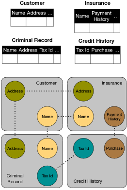
Figure 3. Relatedness graph of the Insurance data silo.

3.3. Profiles as Initial Features

Initialization requirement of GNNs. With SiMa we opt for applying the GraphSAGE model using the relatedness graphs of the corresponding data silos. For this to be possible two conditions should be satisfied about the graph upon which the model will train: i) there should be a representative set of edges and ii) each node should come with an initial feature vector. SiMa’s relatedness graphs already satisfy the first condition, since every such graph includes edges denoting similar columns. Yet, nodes in the relatedness graphs are featureless. Moreover, in order to leverage GNNs and use them for federating data silos, we need to employ them towards a specific goal. Therefore, in the following we discuss how to produce initial features for each column-node in a relatedness graph, and present a method of using a GNN model for bridging data silos by modeling our problem as a link prediction task.

Initial feature vectors from data profiles. In order to handle the feature initialization requirement, in SiMa we draw inspiration from the data profiling literature (Abedjan et al., 2015). In the case of tabular data, profiles summarize the information of a data element, by calculating a series of simple statistics (e.g. number of null values, aggregates etc.). Consequently, we can utilize a simple profiler in order to associate each column in a data silo to a feature vector, summarizing statistical information about it.

In specific, for each data silo, we feed all the including tables into the profiling component we adopt from (Hulsebos et al., 2019). However, since we need the initial profiles to summarize simple information for each column (so as not to depend on complex profiles), we exclude the features referring to pre-trained value and paragraph embeddings. In short, SiMa computes a feature vector for each column in a silo by collecting the following:

– Global statistics. Those include aggregates on high level characteristics of a column, e.g. number of numerical values among the included instances.

– Character-level distributions. For each of the 96 ASCII characters that might be present in the corresponding values of the column, we save charachter-level distributions. Specifically, the profiler counts the number of each such ASCII character in a column and then feeds it to aggregate functions, such as mean, median etc.

Using the above profiling scheme, we associate each node $v$, belonging to a relatedness graph $RG_{i}$, with a vector $\textbf{f}_{v}$. This $\textbf{f}_{v}$ will serve as $\textbf{h}^{0}_{v}$ for initializing the feature vector of $v$ before starting the GraphSAGE training process, as shown in Figure 2b.

3.4. Training GNNs for Federating Silos

Silo federation as link prediction. In order to leverage the capabilities of a GNN, there should be an objective function tailored to the goal of the problem that needs to be solved. With SiMa we want to be able to capture relatedness for every pair of columns belonging to different data silos, which translates to the following objective.

Problem 3.1 (Link prediction of relatedness graph).

Consider a set of relatedness graphs $\mathcal{RG}$, the challenge of link prediction across relatedness graphs is to build a model $\mathcal{M}$ that predicts whether there should be an edge between nodes from different relatedness graphs. Given a pair of nodes $(u,v)$ from two different relatedness graphs $RG_{i},RG_{j}\in\mathcal{RG}$ ($i\neq j$) where $u\in RG_{i}$, $v\in RG_{j}$, ideally

$$\begin{split}\mathcal{M}(u,v)=\begin{cases}1,&u\ and\ v\ are\ linked\\ 0,&otherwise\end{cases}\end{split}$$

By comparing the above problem definition with Problem 2.1, it is easy to see that we have transformed our initial data silo federation problem to a link prediction problem over the relatedness graphs.

Two types of edges for training. Towards this direction, we train a prediction function $\phi$ that receives as input the representations $\textbf{h}_{u}$ and $\textbf{h}_{v}$, of the corresponding nodes $u$ and $v$, from the last layer of the GraphSAGE neural network, and computes a similarity score $sim(u,v)=\phi(\textbf{h}_{u},\textbf{h}_{v})$.

To train a robust GNN model, we need the following two types of edges in our relatedness graph.

Definition 3.2 (Positive edges and negative edges).

In a relatedness graph $RG_{i}=(V_{i},E_{i})$, we refer to each edge $e\in E_{i}$ as a positive edge; if a ‘virtual’ edge $e$ connects two unrelated nodes $u$ and $v$, we refer to it as a negative edge. Thus, we obtain the following two sets of edges.

Positive edges $PE_{i}=\{(u,v)|r(u,v)=1\wedge u,v\in RG_{i}\}$     

Negative edges $NE_{i}=\{(u,v)|r(u,v)=0\wedge u,v\in RG_{i}\}$

To differentiate with negative edges $NE_{i}$, in what follows, we refer to the edges of a relatedness graph $V_{i}$ as positive edges $PE_{i}$. Notably, the training samples we get from our relatedness graphs contain only pairs of nodes for which a link should exist (i.e., positive edges $PE_{i}$). Thus, we need to provide the training process with a corresponding set of negative edges, which connect nodes-columns that are not related. To do so, for every relatedness graph $RG_{i}$ we construct a set of negative edges $NE_{i}$, since we know that nodes belonging to different connected components in $RG_{i}$ represent pairs of unrelated columns in the corresponding data silo $S_{i}$; we elaborate on negative edge sampling strategies in Section 4.1.

Two-fold GNN model training. After constructing the set of negative edges, we initiate the training process with the goal of optimizing the following cross-entropy loss function:

(2) $$\mathcal{L}=-\sum_{(u,v)\in RG_{i}}{\log{\sigma(sim(u,v))}}-\sum_{(u,v)\in NE_{i}}{\big{[}1-\log(\sigma(sim(u,v)))\big{]}},$$

where $\sigma(\cdot)$ is the sigmoid function and $1\leq i\leq n$, with $n$ representing the number of relatedness graphs (constructed from the original data silos) included in training data. The similarity scores are computed by feeding pairs of node representations to a Multi-layer Perceptron (MLP), whose parameters are also learned during the training process in order to give correct predictions. Intuitively, with this model training we want to compute representations of the nodes residing in each relatedness graph (through the training of the GNN), so as to build a similarity function (through the training of the MLP) that based on these, correctly distinguishes semantically related from unrelated nodes-columns.

To summarize, SiMa uses a two-fold model, which consists of:

• A GraphSAGE neural network that applies message passing and aggregation (Equation 1) in order to embed the nodes-columns of the relatedness graph into a vector space of given dimensions.

• A MLP, with one hidden layer, which receives in its input a pair of node representations and based on them it calculates a similarity score in order to predict whether there should be a link or not between them, i.e., whether the corresponding columns are related.

In the above model, there can be certain modifications with respect to the kind of GNN used (e.g. replace GraphSAGE with the classical Graph Convolutional Network (Kipf and Welling, 2016)) and prediction model (e.g. replace MLP by a simple dot product model). However, since the focus of this work is on building a method which uses GNNs as a tool towards data silo federation, and not on comparing/proposing novel GNN-based link prediction models, we opt for a model architecture similar to the ones employed for link prediction (Vretinaris et al., 2021; Ying et al., 2018).

1

2

Input : Set of data silos $\mathcal{S}$

Model $\mathcal{M}$

Profiler $\mathcal{P}$

Number of training epochs $e$

Output : Trained model $\mathcal{M}$

3

$\mathcal{RG}\leftarrow\{\}$ // Initialize set of relatedness graphs

$\text{f}\leftarrow[]$ // List of initial node feature vectors

4

5$n\leftarrow|\mathcal{S}|$

6for $i\leftarrow 1$ to $n$ do

7       $RG_{i}\leftarrow\text{ConstructGraphFromSilo}(S_{i})$

8      $\mathcal{RG}.\text{add}(RG_{i})$

9      foreach node $u\in RG_{i}$ do

             f_u $\leftarrow\mathcal{P}(u)$ // Compute profile of corresponding column and store it as u’s initial feature vector

10             f.append(f_u)

11       end foreach

12      

13 end for

14

$\mathcal{PE},\mathcal{NE}\leftarrow\{\}$ // Initialize sets of positive/negative edges

15

16for $i\leftarrow 1$ to $n$ do

17       foreach edge $(u,v)\in RG_{i}$ do

18            $\mathcal{PE}.\text{add}((u,v))$

19       end foreach

20      

21      $\mathcal{NE}.\text{union}(\text{SampleNegativeEdges}(RG_{i}))$

22 end for

23

24for $i\leftarrow 1$ to $e$ do

       h $\leftarrow\mathcal{M}$.GraphSage($\mathcal{RG}$, f) // Apply GraphSAGE to all relatedness graphs and get node embeddings

       $PosEdgePred\leftarrow\mathcal{M}.$MLP($\mathcal{PE}$, h) // Get link predictions for positive edges

25      

      $NegEdgePred\leftarrow\mathcal{M}.$MLP($\mathcal{NE}$, h) // Get link predictions for negative edges

26      

      Loss$\leftarrow$ComputeLoss($PosEdgePred$, $NegEdgePred$) // Compute cross-entropy loss based on predictions

27      

      Loss.BackPropagate($\mathcal{M}$.parameters) // Tune model parameters with backwards propagation

28      

29 end for

30

Algorithm 1 SiMa

3.5. SiMa’s Pipeline

In Algorithm 1 we show the pipeline that we employ with SiMa. The key challenge here is to build a model that can represent columns of data silos in such a way, so that relatedness prediction based on them is correct. Our method has four inputs: i) the set of data silos $\mathcal{S}$, ii) our defined model $\mathcal{M}$, including the GraphSAGE neural network and the MLP predictor, iii) the profiler $\mathcal{P}$ that we use in order to initialize feature vectors of nodes, and iv) the number of training epochs $e$. The output of SiMa consists of the trained model $\mathcal{M}$, which can then be used to embed any column of a data silo and, based on these embeddings, predict links between columns.

Initially, all data silos in $\mathcal{S}$ are transformed to their relatedness graph counterpart. In addition, we compute the corresponding profiles of each node and store them as initial feature vectors (lines 4-11). Based on these graphs, we construct the sets of positive and negative edges to feed our training process (lines 13-18). While getting positive edges is trivial, since we just fetch the edges that are present in the relatedness graphs, constructing a set of negative edges entails a sampling strategy (line 17). This is because the set of all negative edges is orders of magnitude larger than the set of positive ones. Ergo, we need to sample some of these negative edges in order to balance the ratio of positive to negative examples for our training. We elaborate on our optimized strategies for negative edge sampling in Section 4.1.

Following the preparation of positive and negative edge training samples, we move to the training of our model (lines 19 - 25). In specific, we start by applying the current GraphSAGE neural network through the message passing and aggregation functions shown in Equation 1. At the next step, we get the predictions for the pairs of nodes in the set of positive and negative edges respectively (lines 21-22), by placing in the input of our defined MLP architecture their corresponding embeddings. Finally, the cross-entropy loss is calculated (Equation 2) based on all predictions made for both positive and negative edges (line 23) and based on it we back propagate the errors in order to tune the parameters of the GraphSAGE and MLP models used (line 24). The training process repeats for the number of epochs $e$, which is specified in the input. In the end of this loop, we get our trained model $\mathcal{M}$ which is able to embed columns in data silos and, based on these representations, predict whether they are related or not.

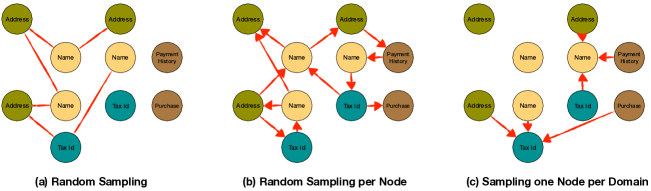
Figure 4. Strategies for negative edge sampling on the relatedness graph of the insurance data silo.

4. Optimizing GNNs for Matching

In this section, we present two novel optimization techniques applied in Algorithm 1: i) the negative edge sampling (Section 4.1) and ii) incremental model training (Section 4.2).

4.1. Negative Sampling Strategies

Since the number of possible negative edges in our relatedness graphs might be overwhelming with respect to the number of positive edges, we need to devise negative sampling strategies. In fact, negative sampling for graph representation learning has been shown to drastically impact the effectiveness of a model (Yang et al., 2020). However, since we do not want to add more complexity to our model, with SiMa we want to introduce simple, yet effective, sampling techniques which provide with negative edge samples that help our link prediction model distinguish related/dissimilar columns. Thus, in the following we describe three negative sampling strategies (termed as NS1, NS2, NS3), each enhanced with meaningful insights. It is important to mention here that these negative sampling techniques take place inside every relatedness graph, wherein we have the knowledge about which node pairs represent negative examples. To illustrate how these strategies proceed, in Figure 4 we depict each one of them on the relatedness graph in Figure 3.

NS1: Random sampling on whole graph. The most straightforward and simple way to compute a sample of negative edges per relatedness graph, is to randomly sample some of them out of the set of all possible negative node pairs. In specific, based on the node connectivity information we have about each relatedness graph, we are able to compute the full set of distinct pairs which include nodes from different connected components; these represent columns in the original data silo that are not related. Then, we simply extract a sample of these negative edges by randomly picking some of them in order to construct a set with a size equal to the number of positive edges in the corresponding relatedness graph, to avoid overfitting.

Now we explain the drawbacks of this sampling strategy with the example in Figure 4a. Figure 3 depicts six positive edges in the relatedness graph, while Figure 4a shows the six randomly selected negative edges. A major drawback is that there could be nodes not connected with any negative edge in the sample, like the three rightmost nodes in the figure. This could severely affect the training process, since for these nodes we miss information about nodes they should not relate to. Moreover, it might be that certain nodes show up more frequently in the negative samples than others, which creates an unwanted imbalance in the training data for negative examples.

NS2: Random sampling per node. In order to deal with the shortcomings of the previous sampling strategy, we propose proceeding with random sampling per node in the relatedness graph. Specifically, in order to guarantee that every node is associated with at least one negative edge, we randomly sample negative edges for each node separately. To balance the number of positive and negative edges that a node is associated with, we specify the sample size to be equal to the degree of the node in the relatedness graph, i.e., to the number of positive edges; since we want to control the number of incoming negative edges per node, we choose to sample directed edges. With this optimization we manage not only having negative samples for each node, but also we ensure that the number of incoming positive and negative edges per node will be equal.

Figure 4b shows a possible output of such a negative edge sampling strategy. In contrast to the previous strategy, we see that now every node in the graph receives a sample of directed negative edges, of size equal to its corresponding degree in the original relatedness graph. Nonetheless, this improved sampling strategy does not ensure that a node will receive negative edges from a set of nodes that belong to different connected components, namely different column domains. For example, in Figure 4b the upper left “Address” node receives two edges both coming from the connected component representing the domain of customer names. This non-diversity of the negative samples that are associated with each node, disrupts the learning process since the model does not receive enough information about which columns should not be regarded as related.

NS3: Random sampling per domain. As an optimization to the previous sampling strategy, with which we aim to improve the shortness of diversity in the negative edges each node receives, we impose sampling per node to take place per different domain, i.e., for each different connected component in the relatedness graph. In detail, we proceed with sampling per node, as with NS2, but this time we pick random samples based on each connected component that has not yet been associated to the node. Hence, each node receives at least one negative edge from every other connected component in the graph, ensuring this way that there is diverse and complete information with respect to domains that the corresponding column does not relate. To keep the number of negative edges close to the number of positive ones, we specify one random sample from each domain per node. In cases where the number of negative edges that a node receives (which is equal to the number of all connected components, except for the one it belongs to) is still considerably higher than its associated positive ones, we can further sample to balance the two sets; this sacrifices completeness of information about dissimilar nodes, but still ensures diversity and that the model will not overfit.

To illustrate how the above strategy proceeds, in Figure 4c we show negative samples computed only for two different nodes, “Tax id” and “Name” (we do so in order to not overload the figure with negative edges for all nodes). Indeed, as we discussed above, both of these nodes receive exactly one randomly picked edge from each unrelated domain. Therefore, every node has complete information which can be leveraged by our proposed model in order to learn correctly which pairs of nodes should not be linked.

1

2

3$n\leftarrow|\mathcal{RG}|$ ;

$TG\leftarrow[]$ // TG holds list of relatedness graphs included in the training

4

5for $i\leftarrow 1$ to $n$ do

6       $TG$.append($RG_{i}$) ;

7       for $j\leftarrow 1$ to $e_{p}$ do

             h $\leftarrow\mathcal{M}$.GraphSage($TG_{i}$, f_i) // Apply GraphSAGE only on relatedness graphs in TG

             $PosEdgePred\leftarrow\mathcal{M}.$MLP($\mathcal{PE}_{i}$, h) // Get link predictions for positive edges

8            

            $NegEdgePred\leftarrow\mathcal{M}.$MLP($\mathcal{NE}_{i}$, h) // Get link predictions for negative edges

9            

            Loss $\leftarrow$ ComputeLoss($PosEdgePred$, $NegEdgePred$) // Compute cross-entropy loss based on predictions

10            

            Loss.BackPropagate($\mathcal{M}$.parameters) // Tune model parameters with backwards propagation

11            

12       end for

13      

14 end for

Algorithm 2 Incremental Training

4.2. Incremental Training

Originally, SiMa trains on the positive and negative samples it receives by taking into consideration every relatedness graph in the input (lines 19-25 in Algorithm 1). However, proceeding with training on the whole set of graphs might harm the effectiveness of the learning process, since the model in each epoch trains on the same set of positive and negative samples; hence, it can potentially overfit. Therefore, we need to devise an alternative training strategy, which feeds the model with new training data periodically.

Towards this direction, we design an incremental training scheme that proceeds per relatedness graph. In specific, we initiate training with one relatedness graph and the corresponding positive/negative samples we get from it. After a specific number of epochs, we add the training samples from another relatedness graph and we continue the process by adding every other relatedness graph. In this way, we help the model to deal periodically with novel samples potentially representing previously unseen domains that the new relatedness graph brings; thus, we increase the chances of boosting the effectiveness that the resulting link prediction will have. Essentially, our incremental training scheme resembles curriculum learning (Bengio et al., 2009) in that it constantly provides the learning process with new data; yet, curriculum learning methods also verify that the training examples are of increasing difficulty.

Algorithm 2 shows how incremental training proceeds and replaces the original training scheme in the context of our initial pipeline in Algorithm 1. We see that the only difference with the previous scheme is that now we train the model on an incrementally growing set of relatedness graphs ($TG$ of lines 2), which is initialized with the first relatedness graph and it receives an extra graph, periodically every $e_{p}$ epochs (which we assume to be a fraction of the original number of epochs $e$ in Algorithm 1), until it contains all of them in the final iteration. For each epoch, we apply GraphSAGE only on the relatedness graphs in $TG$ (lines 6) and use positive/negative samples coming from them in order to train the MLP (lines 8-9).

5. Experimental Evaluation

In this section, we assess the effectiveness and efficiency of SiMa through an extensive set of experiments. In what follows, we first describe our experimental setup, namely the datasets, baselines and settings against which we assess our method. We then present our experimental results, where we focus on: i) the effect of our proposed optimizations (Section 4), the ability of SiMa to adapt to different settings, and how well it competes with the state-of-the art matching baselines, both in terms of effectiveness and efficiency.

5.1. Setup

Matching baselines. In order to compare SiMa against the state-of-the art matching techniques, we employ Valentine (Koutras et al., 2021b), an openly available experiment suite, which consolidates several state-of-the-art matching methods. We choose the instance-based methods included in Valentine, since those have been shown to work substantially better than the schema-based ones. Namely:

• COMA (Do and Rahm, 2002), which is a seminal matching method that combines multiple matching criteria in order to output a set of possible matches. We make use of the COMA version that uses both schema and instance-based information about the datasets in order to proceed.

• Distribution-based matching (Zhang et al., 2011), where relationships between different columns are captured by comparing the distribution of their respective data instances.

• EmbDI (Cappuzzo et al., 2020), which is a state-of-the-art making use of locally embeddings. As discussed in Section 6 EmbDI can be used for matching tabular data.

• Jaccard-Levenshtein matcher, which is a simple baseline that computes Jaccard similarity between the instance sets of column pairs, by assuming that values are identical if their Levenshtein distance is below a given threshold.

Benchmark	Size	# Silos	# Datasets/Silo (Min, Max, Increment)
OpenData (Nargesian et al., 2018)	large	8	[10, 80, 10]
	medium	4	[6, 24, 6]
	small	2	[4,10,6]
GitTables (Hulsebos et al., 2021)	large	10	[10, 100, 10]
	medium	5	[4,20, 4]
	small	2	[4,10,6]

Table 2. Data Silo configurations for each of our constructed benchmarks.

In addition to those, we also devise another two simple baselines:

• Profile-based matching, where we use the initial profiles of the columns in order to compute exhaustively cosine-similarities for every possible column pair, and

• Pre-trained embeddings matching, which computes for every column an embedding based on a pre-trained model on natural language corpora from fastText (Bojanowski et al., 2017), and then proceeds in a similar way as the previous baseline.

Therefore, the matching baselines we include in our experimental setup represent some of the best efforts in the matching literature. Since the methods were shown to cover the spectrum of matcher types that related dataset search methods use (Koutras et al., 2021b), our set of baselines covers is complete and a fair choice for comparing against existing solutions, as discussed in Section 2.

Datasets. In order to simulate settings of different data silos that share links, but also contain extra information each, we need a considerable amount of real-world alike datasets. Towards this direction, we use the dataset fabricator provided by Valentine (Koutras et al., 2021b, a), which produces pairs of tabular datasets that share a varying number of columns/rows. Importantly, the fabricator can also perturb data instances and distributions in order to provide with challenging scenarios. Therefore, we create the following two benchmarks, :

• OpenData (Nargesian et al., 2018) - 800 datasets. This benchmark consists of tables from Canada, USA and UK Open Data, as extracted from the authors of (Nargesian et al., 2018). The tables represent diverse sources of information, such as timetables for bus lines, car accidents, job applications, etc. We use 8 source tables, and produce 100 fabricated ones from each.

• GitTables (Hulsebos et al., 2021) - 1000 datasets. In this benchmark we include datasets drawn from the GitTables project (Hulsebos et al., 2021), which encompasses 1.7 million tables extracted from CSV files in GitHub. Specifically, we fabricate 1000 datasets from 10 source tables (100 datasets per source table), which store information of various contexts, such as reddit blogs, tweets, medical related data, etc.

Each of these benchmarks comes with its own ground truth of matches that should hold among the columns of different datasets. Ground truth was produced automatically for datasets fabricated from the same source table, and manually for pairs of columns belonging to datasets of different domains.

Since our goal is to construct sets of data silos, which share related columns but also contain dataset categories that are unique to each, we proceed as follows for each of the above benchmarks: we set a number of silos, and then in the first one we include a sample of datasets originating from only a fraction of the existing dataset domains, in the next one we add also datasets from other domains, and so on and so forth; hence, the last silo contains datasets from each possible category included in the corresponding benchmark. In this way, we manage to create silos that have multiple links across them, while they incrementally store datasets from a larger pool of domains.

Dataset sizes. During our experimentation we observed that two of the matching methods pose scalability issues. Specifically both Distribution-based matching (Zhang et al., 2011) and EmbDI (Cappuzzo et al., 2020) were not able to finish within a reasonable time during our experiments (e.g., EmbDI took more than 2 days to complete even for small configurations of two silos and 14 datasets, as shown in Figure 5). For this reason, we created three silo scenarios per benchmark with growing size: small, medium and large, so that we can run all matching baselines. While increasing the sizes of our silo scenarios, we ensure that datasets included in the smaller ones are also part of the bigger ones, i.e., small $\subset$ medium $\subset$ large. In Table 2 we present each data silo configuration characteristics that we construct from our dataset benchmarks, where we show the number of silos and the sizes of the smallest and largest one respectively (together with the increment in size for silos in between).

Effectiveness calculation. We evaluate the effectiveness of our method by calculating Precision, Recall and F1-score based on the predictions we get for every possible pair of columns belonging to datasets of different silos. In particular, we assume that SiMa predicts that there should be a relationship between two columns, if the corresponding similarity score we get from the MLP of our model is greater than 0.5. Then, calculation of Precision, Recall and F-measure proceeds in the traditional way based on the confusion matrix. The effectiveness of the matching baselines we compare against is calculated based on the ranked list of similarities they output for each column pair of datasets belonging to different silos. In order to evaluate them in a similar way as SiMa we normalize their similarity results and assume again that two columns match if their normalized similarity score is above 0.5.

Strategies	NS1 - Inc.Training			NS2 - Inc Training			NS3 - Inc. Training			NS3 - Non-inc. Training
Data Silos	Precision	Recall	F1	Precision	Recall	F1	Precision	Recall	F1	Precision	Recall	F1
OpenData-large	0.62	0.85	0.72	0.80	0.93	0.86	0.94	0.94	0.94	0.32	0.67	0.44
GitTables-large	0.60	0.69	0.65	0.65	0.75	0.69	0.81	0.82	0.82	0.38	0.51	0.43

Table 3. Effect of negative sampling and incremental training strategies

Implementation details. For our GraphSAGE model we use one layer (i.e. each node receives information only by its immediate neighbors) and set the dimension of produced embeddings to 300; the MLP we use has one hidden layer. Each node in the graph uses max-pooling to aggregate the representations of its neighborhood nodes, as described in (Hamilton et al., 2017). For the matching baselines we compare with from Valentine, we use the default parameters as stated in (Koutras et al., 2021b). In addition, we set the number of epochs $e$ to be equal to 300; in the case of incremental training we break this number into equal intervals based on the number of relatedness graphs, e.g. if $|\mathcal{RG}|=10$ then $e_{p}$ in Algorithm 2 is equal to 30. For training we use the Adam optimizer (Kingma and Ba, 2014) with a learning rate of 0.01. Furthermore, our method is implemented in Python 3.7.4 and is openly available for experimenation, while GraphSAGE was implemented using the Deep Graph Library (Wang et al., 2019) on top of PyTorch. Experiments for SiMa ran on a 16-core VM linux machine. To get results from our matching baselines we set up a cluster containing Google Cloud Platform’s e2-standard-16 and n1-standard-64 machines.

Methods	SiMa			COMA
Data Silos	Precision	Recall	F1	Precision	Recall	F1
OpenData-large	0.94	0.94	0.94	0.99	0.58	0.73
GitTables-large	0.81	0.82	0.82	0.89	0.87	0.88
Methods	SiMa			Distribution-based
Data Silos	Precision	Recall	F1	Precision	Recall	F1
OpenData-medium	0.84	0.79	0.81	0.73	0.58	0.65
GitTables-medium	0.88	0.76	0.82	0.92	0.48	0.63
Methods	SiMa			EmbDI
Data Silos	Precision	Recall	F1	Precision	Recall	F1
OpenData-small	0.71	0.72	0.72	0.18	0.74	0.28
GitTables-small	0.77	0.83	0.80	0.09	0.88	0.17

Table 4. Effectiveness of SiMa vs SotA matching methods. In principle, SotA matching methods are inapplicable to the problem of data silo federation because they require global access to all data, but even if they could be used, SiMa would still outperform them both in effectiveness and efficiency (Figure 5).

5.2. Effectiveness of Optimizations

We assess the effectiveness of our optimizations, as discussed in Section 4, in order to verify their validity. Towards this direction, we run two sets of experiments: i) using the incremental training scheme, we apply three variants of SiMa, based on a different negative sampling strategy, and ii) using the best such negative sampling scheme, we compare SiMa’s incremental training against training on the whole set of relatedness graphs we get from the data silos. Both types of experiments were run on the large size data silo configurations, as constructed from our two benchmarks.

In Table 3 we see the evaluation results for the three negative sampling strategies, as introduced in Section 4.1. In detail, we verify that random sampling of edges from each relatedness graph, as specified by NS1, produces the worst effectiveness results in both data silo settings. This is because negative edges sampled with this strategy do not cover all nodes of each corresponding relatedness graph. Since the second sampling strategy (NS2) deals with this problem by specifying random samples per node, the effectiveness results we get by employing it are better, both in terms of precision and recall; feeding each node with at least one negative edge, helps it receive information about other nodes that should not share a link with, and thus improve the prediction accuracy of SiMa’s model. Yet, we see that precision is still mediocre and improvements are minor with respect to NS1, due to the lack of diversity and completeness about the knowledge each node receives about other domains in the relatedness graph.

On the other hand, we validate the boost in effectiveness that sampling edges from each other domain per node, i.e. NS3, can bring. In particular, we see a considerable improvement in both precision and recall, since with NS3 every node receives negative edges that cover the spectrum of other domains present in the corresponding relatedness graph. Consequently, the false positive links that our method predicts decrease (i.e. precision increases), while the better representational quality of the embeddings produced by our encapsulated GraphSAGE model ensures fewer false negatives (i.e. recall increases).

Finally, we verify that incremental training has a substantial influence on the effectiveness of the training process. Specifically, we observe that training on all relatedness graphs from the beginning can severely affect the effectiveness of our method, since our model overfits on the set of possible and negative samples it receives. On the contrary, our incremental training scheme drastically helps our model to adapt to new examples and significantly improves its prediction correctness. Indeed, by applying SiMa’s model on every relatedness graph incrementally, we guarantee that the learning process will leverage the novel information that each graph brings, i.e. novel examples of semantic types that were not introduced by the previous graphs. Therefore, in the following experiments we configure SiMa to apply the incremental training scheme and use NS3 as the negative edge sampling strategy.

5.3. SiMa vs SotA Matching & Baselines

Effectiveness comparison. The upper part of Table 4 contains the effectiveness comparison of SiMa with COMA (Do and Rahm, 2002), on the large data silo configurations. In the case of OpenData, we see that SiMa has a superior F1-score, since both its precision and recall scores are high; hence, our model seems to learn significantly well how to disambiguate between positive and negative links, based on the knowledge that exists in each data silo. On the other hand, while COMA’s precision is close to 1, i.e. almost all the matches it predicts are correct, we see that its recall is quite low. This should be due to the complexity of open data, which makes it difficult for traditional matching techniques like COMA to capture relevance among data that might have discrepancies in the way they are formatted (e.g. different naming convention for country codes).

Moving to the GitTables silos, we see that COMA gives slightly better results than SiMa. This is mainly because its recall is higher than in the previous configuration, since relevant data in this benchmark stand out (value formats are almost similar). Nonetheless, SiMa is still highly effective and balanced with regard to its precision and recall; our model is able to capture both relatedness and dissimilarity among column pairs of different silos in both dataset categories.

Comparison with the Distribution-based matcher took place on the medium size data silos, in order to afford the resources this method needed for execution. Based on the results we see in the middle of Table 4, we observe that SiMa is considerably better in terms of effectiveness in both dataset settings. Again, we see that our approach is consistent with respect to precision and recall results, while the Distribution-based method suffers from low recall; distribution similarity does not help towards finding the majority of correct matches among silos. Conversely, SiMa is still able to leverage the relationship information inside silos in order to build a model that can disambiguate between columns that should be related and others that should not.

To be able to compare our method against EmbDI, we ran experiments on the small size data silos, since scaling this method towards matching multiple datasets is quite resource-demanding. By looking into the comparison results with our method (bottom of Table 4), we see that SiMa is significantly more effective and reliable. Surprisingly, even if the knowledge of relationships inside each data silo in the small settings is quite less than the large and medium ones, our method still manages to capture relatedness sufficiently well. On the contrary, EmbDI shows very low precision since the majority of matches it returns refer to false positives; this is due to the construction of training data, where even columns that should not be related share the same context, hence EmbDI embeds them very close in the vector space.

Other baselines. The comparisons with the Jaccard Levenshtein, Profile-based and Pre-trained embeddings matching baselines are excluded for the sake of space, since their effectiveness was considerably low.

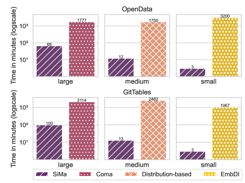
Figure 5. Efficiency of SiMa vs SotA methods.

Efficiency comparison. In Figure 5, we see how SiMa compares with state-of-the-art matching methods in terms of efficiency (i.e. total execution time of each method’s pipeline) measured in minutes and shown in log scale. First and foremost, we observe that SiMa is considerably cheaper than any of the traditional matching methods; indeed, it is 1 (against COMA) to 2 (against Distribution-based and EmbDI) orders of magnitude faster. SiMa’s runtime is dominated by the computation of profiles (roughly $98\%$ of total execution), hence in the case where these are pre-computed our method can give results in a small fraction of the time shown in the figure. Moreover, we verify that applying matching with the state-of-the-art methods, in this scale, might be unaffordable, since it requires access to a lot of resources; in real-world scenarios where multiple data silos of variable sizes need to be federated this can be prohibitively expensive. Interestingly enough, training local embeddings (EmbDI) can be considerably inefficient due to the cost of training data construction (i.e., graph construction, random walk computation). On the other side, calculating distribution similarity among columns is computationally heavy, while COMA’s syntactic-based matching can be slow due to computations of various measures among instance sets of columns (e.g. TF-IDF).

Summary. SiMa is at least as effective as state-of-the-art schema matching methods. This is because its effectiveness does not depend on assumptions about the format of values in the different data silos (like traditional matching methods), since it leverages the knowledge that already exists in each of them. At the same time, SiMa is significantly more efficient (20x to 1000x faster) than traditional matching methods, as it avoids computations among all datasets of different silos. Finally, it is important to stress that in the silo matching scenario, SiMa is the only applicable method, as it can match without having access to all datasets at the same time – SiMa’s models can be trained incrementally.

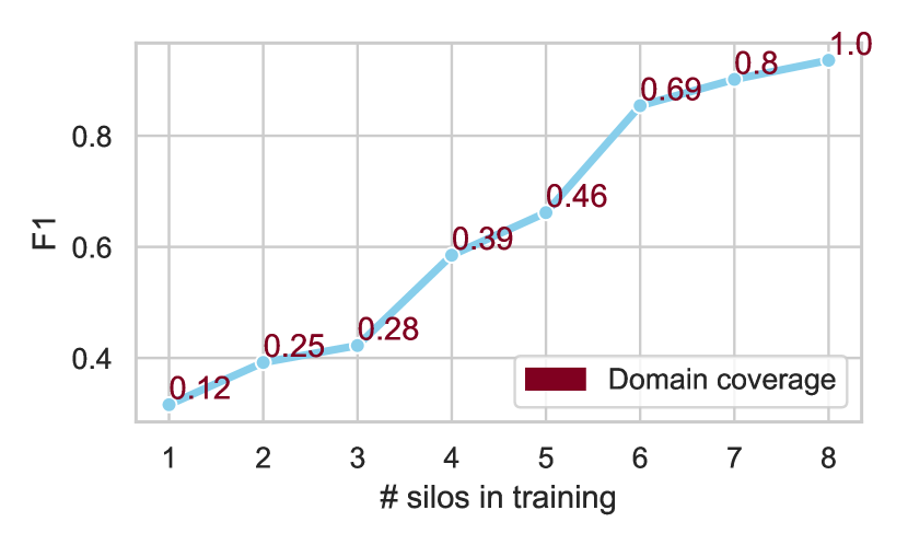
Figure 6. Generalizability of SiMa with respect to number of silos participating in the training.

5.4. Generalizability of SiMa

SiMa has the ability to generalize on datasets unseen during training since the GNN model we use (i.e. GraphSAGE) is inductive, namely it can be used to embed nodes of relatedness graphs that did not participate in the learning process. In particular, we do so by measuring the effectiveness of SiMa when applied for capturing relatedness among all data silos, while gradually increasing the number of silos participating in the training (i.e., we initially include the first one, then the second one etc.). This way we can control the percentage of column domains (with respect to all the datasets across all silos) that the model trains upon each time.

In Figure 6 we show how well our method’s model can generalize on data silos that were not part of the input, in the case of the OpenData-large configuration (without loss of generality). Specifically, we illustrate how the F1-score changes with the addition of more silos in the training data (the numbers next to each point represent the corresponding column domain coverage). As expected, we see that when we include only a few data silos and, hence, a small percentage of column domains in the training (less than $50\%$), the effectiveness of SiMa is low (F1-score $\leq 70\%$). Nonetheless, we observe that SiMa generalizes very well to unseen data (F1-score $\geq 85\%$) when the learning process includes columns that cover at least $70\%$ of domains. Therefore, even if we apply our model to new data that were not part of the method’s training, in the case where we are not willing to retrain our model on new data silos, it is possible to get a considerably high amount of correct predictions. However, we believe that retraining on new data is a better option, regarding the gains in effectiveness; training on new data is not very costly, since SiMa can be trained incrementally.

6. Related Work

Schema matching. A natural choice to bridge data silos would be to employ schema matching (Rahm and Bernstein, 2001; Gal, 2011), namely a set of methods responsible for finding matches among elements of disparate datasets based on various similarity criteria (e.g. Jaccard similarity). Schema matching is a well-studied research topic, with various methods mainly focusing on finding matches between pairs of tables (Do and Rahm, 2002; Madhavan et al., 2001; Zhang et al., 2011; Cappuzzo et al., 2020), Yet, despite the wealth of literature, scaling state-of-the-art schema matching methods horizontally is very resource-intensive: performing matching for all possible column pairs of disparate tables, residing in different silos is a task of quadratic time complexity with respect to the number of columns. Moreover, recent works show that they are not as effective as expected, while they might be inefficient even when processing limited numbers of dataset pairs (Koutras et al., 2021b).

Related dataset search. Related dataset search methods (Fernandez et al., 2018a; Cafarella et al., 2009; Das Sarma et al., 2012; Nargesian et al., 2018; Zhu et al., 2019; Bogatu et al., 2020; Zhang and Ives, 2020) methods introduce techniques that are based on criteria such as syntactic, distribution or even embedding similarity of values residing in the corresponding columns. To increase performance, the majority of them make use of dedicated search structures, such as LSH indexes (Nargesian et al., 2018; Fernandez et al., 2018a; Bogatu et al., 2020) or inverted indexes (Zhu et al., 2019); by accessing these structures, they can provide ranked lists to top-k queries on a dataset or column level. However, using such methods for federating data silos is improper, since they are optimized for a problem of different nature. Specifically, in the case of data silo federation, we are concerned on capturing all potential relationships between columns coming from datasets of different silos and not on finding the top-k relevant datasets/columns to a given one.

Embedding-based methods. Recently several (solely or partially) embedding-based methods have emerged, which can be applied in matching. Despite their seamless employment for embedding cell-values, and consequently table columns (Fernandez et al., 2018b; Nargesian et al., 2018), pre-trained models have been shown to not generalize well on domain-specific datasets (Koutras et al., 2021b). On the other hand, locally-trained embedding methods (Fernandez and Madden, 2019; Koutras et al., 2020; Cappuzzo et al., 2020) leverage the architecture of skip-gram models (Mikolov et al., 2013; Bojanowski et al., 2017) to train on corpora consisting of tabular data. While training on the tables residing in different data silos can be an improvement with respect to simply using pre-trained models, locally-trained models still seem to be insufficiently effective when used for matching related columns (Koutras et al., 2021b). In addition, such models require a lot of time and resources for constructing the training data, while they need retraining when there are changes on the datasets (additions/updates/deletions). Thus, employing them in the case where we have frequent data updates, could considerably harm efficiency. Very importantly, mapping every data element (cell values, columns) to a vector representation could lead to massive storage overhead (Fernandez and Madden, 2019).

Column-level type classification. Sherlock (Hulsebos et al., 2019) trains a deep learning model over a large corpus of tables, which can be used to effectively classify columns with respect to a specific set of semantic types, like address, age, city, artist etc. Nonetheless, the method underperforms for types that are not sufficiently represented in the training data, while it only considers values of the columns to proceed with classification. These problems are tackled by its successor Sato (Zhang et al., [n. d.]), which extends Sherlock’s model with column context information. Despite their proven effectiveness on column classification tasks, these methods are not applicable on our setting, since the semantic types and their number are unknown when trying to find links among datasets from different silos; otherwise, we could also transform data silo federation to a classification problem. Moreover, the models of Sherlock and Sato need a considerable amount of training data in order to perform as expected ($\sim$600 K tables), while with SiMa we leverage only the relatedness information in each silo.

7. Conclusion

In this paper, we introduced SiMa, a novel method for federating disparate data silos, which uses an effective prediction model based on the representational power of GNNs. SiMa uses the knowledge about existing relationships among datasets in silos, in order to build a model that can capture potential links across them. Our experimental results show that SiMa can be more effective than current state-of-the-art matching methods, while it is significantly faster and cheaper to employ.

References

- (1)
- Abedjan et al. (2015) Ziawasch Abedjan, Lukasz Golab, and Felix Naumann. 2015. Profiling relational data: a survey. VLDBJ 24, 4 (2015), 557–581.
- Bengio et al. (2009) Yoshua Bengio, Jérôme Louradour, Ronan Collobert, and Jason Weston. 2009. Curriculum learning. In Proceedings of the 26th annual international conference on machine learning. 41–48.
- Bogatu et al. (2020) Alex Bogatu, Alvaro AA Fernandes, Norman W Paton, and Nikolaos Konstantinou. 2020. Dataset Discovery in Data Lakes. In IEEE ICDE.
- Bojanowski et al. (2017) Piotr Bojanowski, Edouard Grave, Armand Joulin, and Tomas Mikolov. 2017. Enriching word vectors with subword information. TACL 5 (2017), 135–146.
- Cafarella et al. (2009) Michael J Cafarella, Alon Halevy, and Nodira Khoussainova. 2009. Data integration for the relational web. In VLDB.
- Cappuzzo et al. (2020) Riccardo Cappuzzo, Paolo Papotti, and Saravanan Thirumuruganathan. 2020. Creating embeddings of heterogeneous relational datasets for data integration tasks. In Proceedings of the 2020 ACM SIGMOD International Conference on Management of Data. 1335–1349.
- Chepurko et al. (2020) Nadiia Chepurko, Ryan Marcus, Emanuel Zgraggen, Raul Castro Fernandez, Tim Kraska, and David Karger. 2020. ARDA: automatic relational data augmentation for machine learning. Proceedings of the VLDB Endowment 13, 9 (2020), 1373–1387.
- Das Sarma et al. (2012) Anish Das Sarma, Lujun Fang, Nitin Gupta, Alon Halevy, Hongrae Lee, Fei Wu, Reynold Xin, and Cong Yu. 2012. Finding Related Tables. In ACM SIGMOD.
- Do and Rahm (2002) Hong-Hai Do and Erhard Rahm. 2002. COMA: a system for flexible combination of schema matching approaches. In VLDB.
- Errica et al. (2019) Federico Errica, Marco Podda, Davide Bacciu, and Alessio Micheli. 2019. A fair comparison of graph neural networks for graph classification. arXiv preprint arXiv:1912.09893 (2019).
- Fan et al. (2019) Wenqi Fan, Yao Ma, Qing Li, Yuan He, Eric Zhao, Jiliang Tang, and Dawei Yin. 2019. Graph neural networks for social recommendation. In The World Wide Web Conference. 417–426.
- Fernandez et al. (2018a) Raul Castro Fernandez, Ziawasch Abedjan, et al. 2018a. Aurum: A data discovery system. In IEEE ICDE.
- Fernandez and Madden (2019) Raul Castro Fernandez and Samuel Madden. 2019. Termite: a system for tunneling through heterogeneous data. In Proceedings of the Second International Workshop on Exploiting Artificial Intelligence Techniques for Data Management. 1–8.
- Fernandez et al. (2018b) Raul Castro Fernandez, Essam Mansour, et al. 2018b. Seeping semantics: Linking datasets using word embeddings for data discovery. In IEEE ICDE.
- Gal (2011) Avigdor Gal. 2011. Uncertain schema matching. Synthesis Lectures on Data Management 3, 1 (2011), 1–97.
- Hamilton et al. (2017) William L Hamilton, Rex Ying, and Jure Leskovec. 2017. Inductive representation learning on large graphs. In Proceedings of the 31st International Conference on Neural Information Processing Systems. 1025–1035.
- Hulsebos et al. (2021) Madelon Hulsebos, Çağatay Demiralp, and Paul Groth. 2021. GitTables: A Large-Scale Corpus of Relational Tables. arXiv preprint arXiv:2106.07258 (2021).
- Hulsebos et al. (2019) Madelon Hulsebos, Kevin Hu, Michiel Bakker, Emanuel Zgraggen, Arvind Satyanarayan, Tim Kraska, Çagatay Demiralp, and César Hidalgo. 2019. Sherlock: A deep learning approach to semantic data type detection. In Proceedings of the 25th ACM SIGKDD International Conference on Knowledge Discovery & Data Mining. 1500–1508.
- Kingma and Ba (2014) Diederik P Kingma and Jimmy Ba. 2014. Adam: A method for stochastic optimization. arXiv preprint arXiv:1412.6980 (2014).
- Kipf and Welling (2016) Thomas N Kipf and Max Welling. 2016. Semi-supervised classification with graph convolutional networks. arXiv preprint arXiv:1609.02907 (2016).
- Koutras et al. (2020) Christos Koutras, Marios Fragkoulis, Asterios Katsifodimos, and Christoph Lofi. 2020. REMA: Graph Embeddings-based Relational Schema Matching. In SEAData.
- Koutras et al. (2021a) Christos Koutras, Kyriakos Psarakis, Andra Ionescu, Marios Fragkoulis, Angela Bonifati, and Asterios Katsifodimos. 2021a. Valentine in Action: Matching Tabular Data at Scale. VLDB 14, 12 (2021), 2871–2874.
- Koutras et al. (2021b) Christos Koutras, George Siachamis, Andra Ionescu, Kyriakos Psarakis, Jerry Brons, Marios Fragkoulis, Christoph Lofi, Angela Bonifati, and Asterios Katsifodimos. 2021b. Valentine: Evaluating Matching Techniques for Dataset Discovery. In 2021 IEEE 37th International Conference on Data Engineering (ICDE). IEEE, 468–479.
- Lehmberg and Bizer (2017) Oliver Lehmberg and Christian Bizer. 2017. Stitching web tables for improving matching quality. In VLDB.
- Madhavan et al. (2001) Jayant Madhavan, Philip A Bernstein, and Erhard Rahm. 2001. Generic schema matching with cupid. In VLDB.
- Mansour et al. (2021) Essam Mansour, Kavitha Srinivas, and Katja Hose. 2021. Federated Data Science to Break Down Silos [Vision]. SIGMOD record (2021).
- Mikolov et al. (2013) Tomas Mikolov, Ilya Sutskever, Kai Chen, et al. 2013. Distributed representations of words and phrases and their compositionality. In NIPS.
- Miller (2018) Renée J Miller. 2018. Open data integration. Proceedings of the VLDB Endowment 11, 12 (2018), 2130–2139.
- Nargesian et al. (2018) Fatemeh Nargesian, Erkang Zhu, Ken Q Pu, and Renée J Miller. 2018. Table union search on open data. In VLDB.
- Rahm and Bernstein (2001) Erhard Rahm and Philip A Bernstein. 2001. A survey of approaches to automatic schema matching. VLDBJ 10, 4 (2001), 334–350.
- Vretinaris et al. (2021) Alina Vretinaris, Chuan Lei, Vasilis Efthymiou, Xiao Qin, and Fatma Özcan. 2021. Medical entity disambiguation using graph neural networks. In Proceedings of the 2021 International Conference on Management of Data. 2310–2318.
- Wang et al. (2019) Minjie Wang, Da Zheng, Zihao Ye, Quan Gan, Mufei Li, Xiang Song, Jinjing Zhou, Chao Ma, Lingfan Yu, Yu Gai, et al. 2019. Deep graph library: A graph-centric, highly-performant package for graph neural networks. arXiv preprint arXiv:1909.01315 (2019).
- Wu et al. (2020) Zonghan Wu, Shirui Pan, Fengwen Chen, Guodong Long, Chengqi Zhang, and S Yu Philip. 2020. A comprehensive survey on graph neural networks. IEEE transactions on neural networks and learning systems 32, 1 (2020), 4–24.
- Yang et al. (2020) Zhen Yang, Ming Ding, Chang Zhou, Hongxia Yang, Jingren Zhou, and Jie Tang. 2020. Understanding negative sampling in graph representation learning. In Proceedings of the 26th ACM SIGKDD International Conference on Knowledge Discovery & Data Mining. 1666–1676.
- Ying et al. (2018) Rex Ying, Ruining He, Kaifeng Chen, Pong Eksombatchai, William L Hamilton, and Jure Leskovec. 2018. Graph convolutional neural networks for web-scale recommender systems. In Proceedings of the 24th ACM SIGKDD International Conference on Knowledge Discovery & Data Mining. 974–983.
- Zhang et al. ([n. d.]) Dan Zhang, Yoshihiko Suhara, Jinfeng Li, Madelon Hulsebos, Ca gatay Demiralp, and Wang-Chiew Tan. [n. d.]. Sato: Contextual Semantic Type Detection in Tables. Proceedings of the VLDB Endowment 13, 11 ([n. d.]).
- Zhang and Chen (2018) Muhan Zhang and Yixin Chen. 2018. Link prediction based on graph neural networks. Advances in Neural Information Processing Systems 31 (2018), 5165–5175.
- Zhang et al. (2011) Meihui Zhang, Marios Hadjieleftheriou, Beng Chin Ooi, et al. 2011. Automatic discovery of attributes in relational databases. In ACM SIGMOD.
- Zhang and Ives (2020) Yi Zhang and Zachary G Ives. 2020. Finding Related Tables in Data Lakes for Interactive Data Science. In ACM SIGMOD.
- Zhu et al. (2019) Erkang Zhu, Dong Deng, Fatemeh Nargesian, and Renée J. Miller. 2019. JOSIE Overlap Set Similarity Search for Finding Joinable Tables in Data Lakes. In ACM SIGMOD.