Abstract

We consider the classical momentum- or velocity-dependent two-dimensional Hamiltonian given by

$$\mathcal{H}_{N}=p_{1}^{2}+p_{2}^{2}+\sum_{n=1}^{N}\gamma_{n}(q_{1}p_{1}+q_{2}p_{2})^{n},$$

where $q_{i}$ and $p_{i}$ are generic canonical variables, $\gamma_{n}$ are arbitrary coefficients, and $N\in\mathbb{N}$. For $N=2$, being both $\gamma_{1},\gamma_{2}$ different from zero, this reduces to the classical Zernike system. We prove that $\mathcal{H}_{N}$ always provides a superintegrable system (for any value of $\gamma_{n}$ and $N$) by obtaining the corresponding constants of the motion explicitly, which turn out to be of higher-order in the momenta. Such generic results are not only applied to the Euclidean plane, but also to the sphere and the hyperbolic plane. In the latter curved spaces, $\mathcal{H}_{N}$ is expressed in geodesic polar coordinates showing that such a new superintegrable Hamiltonian can be regarded as a superposition of the isotropic 1 : 1 curved (Higgs) oscillator with even-order anharmonic curved oscillators plus another superposition of higher-order momentum-dependent potentials. Furthermore, the symmetry algebra determined by the constants of the motion is also studied, giving rise to a $(2N-1)$th-order polynomial algebra. As a byproduct, the Hamiltonian $\mathcal{H}_{N}$ is interpreted as a family of superintegrable perturbations of the classical Zernike system. Finally, it is shown that $\mathcal{H}_{N}$ (and so the Zernike system as well) is endowed with a Poisson $\mathfrak{sl}(2,\mathbb{R})$-coalgebra symmetry which would allow for further possible generalizations that are also discussed.

MSC: 37J35, 70H06, 22E60, 17B62

PACS: 02.30.Ik, 45.20.Jj, 02.20.Sv, 02.40.Ky

Keywords: Integrable systems; Curvature; Sphere; Hyperbolic plane; Curved oscillator; Poisson coalgebras; Integrable perturbations; symmetry algebras

1 Introduction

Classical and quantum momentum- or velocity-dependent Hamiltonian systems have been extensively studied in the literature over many decades mainly due to their relevant, wide and varied physical applications. Without trying to be exhaustive, let us mention that linear momentum-dependent Hamiltonians have been considered from different viewpoints in [2, 3, 4, 5, 6, 7, 8, 9, 10, 11, 12, 13, 14, 15, 16] and quadratic momentum-dependent ones have been analyzed in [17, 18, 19, 20, 21]. In addition, exponentials of momentum-dependent potentials ($V\propto{\rm e}^{-\,p^{2}}$) have also been considered in [22, 23, 24, 25] and another more involved momentum-dependent potential was recently introduced in [26]; see references therein in all the aforementioned works.

Furthermore, from a completely different perspective, we stress that quantum groups [27] have been applied to classical and quantum (super)integrable Hamiltonians through both deformed and undeformed coalgebras in [28, 29]. Following this coalgebra symmetry approach, several classes of momentum-dependent classical Hamiltonians have been constructed in [29, 30, 31, 32] giving rise to quasi-maximally superintegrable systems, i.e. in arbitrary dimension $d$ they are endowed, by construction, with $(2d-3)$ functionally independent constants of the motion (besides the Hamiltonian). Hence one additional constant of the motion is left to ensure maximal superintegrability.

In this paper, we shall consider a large class of two-dimensional (2D) higher-order momentum-dependent systems comprised within the Hamiltonian given by

$$\mathcal{H}_{N}=p_{1}^{2}+p_{2}^{2}+\sum_{n=1}^{N}\gamma_{n}(q_{1}p_{1}+q_{2}p_{2})^{n},$$ (1.1)

where $q_{i}$ and $p_{i}$ are generic canonical variables (with Poisson bracket $\{q_{i},p_{j}\}=\delta_{ij}$), $\gamma_{n}$ are arbitrary coefficients, and the index $N\in\mathbb{N}$. Therefore, as particular cases, we find that for $N=1$ we shall deal with linear momentum-dependent Hamiltonians and for for $N=2$ with quadratic momentum-dependent ones, but when $N>2$ we shall obtain cubic, quartic…momentum-dependent Hamiltonians.

The underlying motivation to consider $\mathcal{H}_{N}$ (1.1) is that this is just the natural generalization (for arbitrary $N$) of the superintegrable classical Zernike system formerly introduced in [33] (see also [34, 35]), which is recovered for $N=2$ with $\gamma_{1}\neq 0$ and $\gamma_{2}\neq 0$. Recall that the original Zernike system is properly quantum [36] and as a quantum superintegrable Hamiltonian has been extensively studied in [37, 39, 38, 34, 35, 40]. Moreover, we observe that the Hamiltonian $\mathcal{H}_{N}$ (1.1) is naturally endowed with a Poisson $\mathfrak{sl}(2,\mathbb{R})$-coalgebra symmetry [31, 29].

The aim of this paper is twofold. On the one hand, we explicitly prove that the Hamiltonian $\mathcal{H}_{N}$ (1.1) is superintegrable for any $N$ and for any value of the coefficients $\gamma_{n}$. And, on the other hand, we apply this result not only to the flat Euclidean plane $\mathbf{E}^{2}$, but also to the curved sphere $\mathbf{S}^{2}$ and the hyperbolic plane $\mathbf{H}^{2}$.

The structure of the paper is as follows. In the next section we review the classical Zernike Hamiltonian on $\mathbf{E}^{2}$ along with its interpretation on $\mathbf{S}^{2}$ and $\mathbf{H}^{2}$ and, furthermore, we describe its underlying Poisson $\mathfrak{sl}(2,\mathbb{R})$-coalgebra symmetry. This allows us to propose $\mathcal{H}_{N}$ (1.1) as its natural generalized Hamiltonian. In Section 3.1 we prove that $\mathcal{H}_{N}$ always determines a superintegrable system on $\mathbf{E}^{2}$ (for any $\gamma_{n}$ and $N$) by obtaining explicitly the constants of the motion, which turn out to be of higher-order in the momenta. The corresponding interpretation on $\mathbf{S}^{2}$ and $\mathbf{H}^{2}$ is performed in Section 3.2. In particular, we introduce the so called geodesic polar coordinates [41, 42, 43], which are the curved generalization of the usual Euclidean polar coordinates. In this way, we show that $\mathcal{H}_{N}$ can alternatively be regarded as a superposition of the isotropic 1 : 1 curved (Higgs) oscillator with even-order anharmonic curved oscillators plus another superposition of higher-order momentum-dependent potentials.

Such general results are illustrated in Section 4 for $N\leq 8$ and, moreover, the associated polynomial symmetry algebra, defined through the constants of the motion, is also computed leading to a $(2N-1)$th-order generalization of the well-known cubic Higgs Poisson algebra [33, 44]. As a byproduct, our results are specifically applied to the classical Zernike Hamiltonian in Section 5, being interpreted as superintegrable perturbations. Their real part of the trajectories are also plotted up to $N=6$.

We remark that the underlying Poisson $\mathfrak{sl}(2,\mathbb{R})$-coalgebra symmetry of $\mathcal{H}_{N}$ naturally suggests further possible generalizations. These open problems along with the application to (1+1)D Lorentzian spacetimes of constant curvature (Minkowskian and (anti-)de Sitter spaces) are discussed in the last section with some detail. To end with, we stress that a quantization of $\mathcal{H}_{N}$ is also addressed in the last section. The guiding idea is to replace the Poisson $\mathfrak{sl}(2,\mathbb{R})$-coalgebra symmetry by a Lie $\mathfrak{gl}(2)$-coalgebra symmetry. Anyhow, serious ordering problems arise in the constants of the motion, so that our proposal for a quantum $\mathcal{H}_{N}$ Hamiltonian also remains as an open problem.

2 The classical Zernike system revisited

The original quantum Zernike system was introduced in [36] and, very recently, deeply analysed in [37, 39, 38, 34, 35, 40] (see also references therein) as a quantum superintegable Hamiltonian. Such a Hamiltonian system is defined on the 2D Euclidean plane $\mathbf{E}^{2}$, which has a potential depending on both linear and quadratic terms on the quantum momenta operators. Its classical counterpart was formerly presented and studied in [33] (see also [34, 35]), which possesses quadratic in the momenta constants of the motion.

The superintegrable classical Zernike system is the cornerstone of our construction of new higher-order superintegrable momentum-dependent classical Hamiltonians on a 2D Riemannian space of constant (Gaussian) curvature $\kappa$, so covering the flat Euclidean space $\mathbf{E}^{2}$ ($\kappa=0$), the sphere $\mathbf{S}^{2}$ ($\kappa>0$) and the hyperbolic or Lobachevski space $\mathbf{H}^{2}$ ($\kappa<0$). With this aim, we review in this section the main results on the known classical Zernike system along with its interpretation on curved spaces and, furthermore, we present new properties related with Poisson $\mathfrak{sl}(2,\mathbb{R})$-coalgebra symmetry [28, 31, 29, 45, 46] which, to the best of our knowledge, have not been considered in the literature yet.

The main superintegrability properties (in the Liouville sense [47]) of the classical Zernike system are established in the following statement.

Theorem 1.

[33] Let $\{q_{1},q_{2},p_{1},p_{2}\}$ be a set of canonical variables with Poisson brackets $\{q_{i},p_{j}\}=\delta_{ij}$. The classical Zernike Hamiltonian on the Euclidean plane, $(q_{1},q_{2})\equiv(x,y)\in\mathbb{R}^{2}$, is given by

$$\mathcal{H}_{\rm Zk}=p_{1}^{2}+p_{2}^{2}+\gamma_{1}(q_{1}p_{1}+q_{2}p_{2})+\gamma_{2}(q_{1}p_{1}+q_{2}p_{2})^{2},$$ (2.1)

where $\gamma_{1}$ and $\gamma_{2}$ are arbitrary parameters.

(i) The Hamiltonian $\mathcal{H}_{\rm Zk}$ has three (quadratic in the momenta) constants of the motion:

$$\mathcal{C}=q_{1}p_{2}-q_{2}p_{1},$$

$$\mathcal{I}=p_{2}^{2}+\gamma_{1}\,q_{2}p_{2}+\gamma_{2}\bigl{(}q_{1}^{2}+q_{2}^{2}\bigr{)}p_{2}^{2},$$ (2.2)

$$\mathcal{I}^{\prime}=p_{1}^{2}+\gamma_{1}\,q_{1}p_{1}+\gamma_{2}\bigl{(}q_{1}^{2}+q_{2}^{2}\bigr{)}p_{1}^{2}.$$

(ii) The above functions fulfil the relation

$$\mathcal{\mathcal{missing}}H_{\rm Zk}=\mathcal{I}+\mathcal{I}^{\prime}-\gamma_{2}\,\mathcal{C}^{2}.$$ (2.3)

(iii) The sets $\{\mathcal{H}_{\rm Zk},\mathcal{I},\mathcal{C}\}$ and $\{\mathcal{H}_{\rm Zk},\mathcal{I}^{\prime},\mathcal{C}\}$ are formed by three functionally independent functions so that $\mathcal{H}_{\rm Zk}$ is a superintegrable Hamiltonian.

(iv) The three functions defined by

$$\mathcal{L}_{1}:=\mathcal{C}/2,\qquad\mathcal{L}_{2}:=\bigl{(}\mathcal{I}^{\prime}-\mathcal{I}\bigr{)}/2,$$

$$\mathcal{L}_{3}:=\{\mathcal{L}_{1},\mathcal{L}_{2}\}=\left(1+\gamma_{2}\bigl{(}q_{1}^{2}+q_{2}^{2}\bigr{)}\right)p_{1}p_{2}+\tfrac{1}{2}\gamma_{1}(q_{1}p_{2}+q_{2}p_{1}),$$ (2.4)

satisfy the Poisson brackets

$$\{\mathcal{L}_{1},\mathcal{L}_{2}\}=\mathcal{L}_{3},\qquad\{\mathcal{L}_{1},\mathcal{L}_{3}\}=-\mathcal{L}_{2},\qquad\{\mathcal{L}_{2},\mathcal{L}_{3}\}=-\mathcal{L}_{1}\left(\gamma_{1}^{2}+2\gamma_{2}\mathcal{H}_{\rm Zk}+8\gamma_{2}^{2}\mathcal{L}_{1}^{2}\right).$$ (2.5)

All the results covered by Theorem 1 can be expressed straightforwardly in polar coordinates $(r,\phi)$ and conjugate momenta $(p_{r},p_{\phi})$, as it was already performed in [34, 33], by means of the usual canonical transformation given by

$$\begin{array}[]{ll}q_{1}=r\cos\phi,&\quad\displaystyle{p_{1}=\cos\phi\,p_{r}-\frac{\sin\phi}{r}\,p_{\phi}},\\[4.0pt] q_{2}=r\sin\phi,&\quad\displaystyle{p_{2}=\sin\phi\,p_{r}+\frac{\cos\phi}{r}\,p_{\phi}}.\end{array}$$ (2.6)

In particular, in these variables the Hamiltonian $\mathcal{H}_{\rm Zk}$ (2.1) and the angular momentum constant of the motion $\mathcal{C}$ (2.2) turn out to be

$$\mathcal{H}_{\rm Zk}=p_{r}^{2}+\frac{p_{\phi}^{2}}{r^{2}}+\gamma_{1}rp_{r}+\gamma_{2}(rp_{r})^{2},\qquad\mathcal{C}=p_{\phi},$$ (2.7)

showing directly the integrability of the system, while $\mathcal{I}$ (or $\mathcal{I}^{\prime}$) (2.2) is an additional integral (or hidden symmetry) determining its superintegrability.

2.1 Interpretation on the sphere and the hyperbolic space

We stress, as it was already pointed out in [33], that the relations (2.5) provide a cubic Higgs algebra [44] (whenever $\gamma_{2}\neq 0$), which is just the symmetry algebra of the integrals of the motion of the well-known Higgs or isotropic curved oscillator on the 2D sphere $\mathbf{S}^{2}$ that has been extensively studied over the last few decades [44, 48, 49, 41, 50, 51, 52, 53, 54, 43, 55, 56, 57, 58] (see also references therein). We also recall that a cubic Higgs-type algebra arises in Kepler–Coulomb systems on $\mathbf{S}^{2}$ and on the 2D hyperbolic space $\mathbf{H}^{2}$ [59]. These facts suggest a natural relationship between the previous interpretation of $\mathcal{H}_{\rm Zk}$ on $\mathbf{E}^{2}$ and an alternative one as a superintegrable Hamiltonian on a 2D curved space as it was mentioned in [34, 33].

Let us consider the terms in $\mathcal{H}_{\rm Zk}$ depending quadratically in the momenta as the free Hamiltonian or kinetic energy of the system, so that the associated metric can then be deduced. From the expression (2.7) in polar variables the underlying 2D non-Euclidean metric reads

$${\rm d}s^{2}=\frac{1}{1+\gamma_{2}r^{2}}\,{\rm d}r^{2}+r^{2}{\rm d}\phi^{2}.$$ (2.8)

Its Gaussian curvature $\kappa$ turns out to be constant and equal to $-\gamma_{2}$ [34]. Hence, according to the sign of the curvature parameter $\kappa=-\gamma_{2}$, we find that the metric (2.8) simultaneously comprises the flat Euclidean space $\mathbf{E}^{2}$ ($\kappa=\gamma_{2}=0$), the sphere $\mathbf{S}^{2}$ ($\kappa>0,\gamma_{2}<0$) and the hyperbolic space $\mathbf{H}^{2}$ ($\kappa<0,\gamma_{2}>0$). Since both initial (arbitrary) $\gamma_{1}$- and $\gamma_{2}$-potentials are essential to deal with the proper Zernike system we shall assume in this section that they are different from zero, so that we shall deal with $\mathbf{S}^{2}$ and $\mathbf{H}^{2}$.

It should be noted that the polar radial coordinate $r$ is no longer a geodesic distance in a curved space with $\kappa\neq 0$ (which is our case now). In order to perform an appropriate geometrical and dynamical interpretation of $\mathcal{H}_{\rm Zk}$ on $\mathbf{S}^{2}$ and $\mathbf{H}^{2}$, let us introduce the so-called geodesic radial coordinate [41, 43, 42], here denoted by $\rho$, which is just the distance along the geodesic joining the origin in the curved space and the particle, keeping unchanged the usual angular coordinate $\phi$. The relationship between $r$ and $\rho$ is given by

$$r={\rm\ \!S}_{\kappa}(\rho),\qquad\kappa=-\gamma_{2},$$ (2.9)

where from now on we shall make use of the curvature-dependent cosine and sine functions defined by [41, 60, 42]

$${\rm\ \!C}_{\kappa}(x):=\left\{\begin{array}[]{ll}\cos{\sqrt{\kappa}\,x}&\quad\kappa>0\\ \qquad 1&\quad\kappa=0\\ \cosh{\sqrt{-\kappa}\,x}&\quad\kappa<0\end{array}\right.,\qquad{\rm\ \!S}{{}_{\kappa}}(x):=\left\{\begin{array}[]{ll}\frac{1}{\sqrt{\kappa}}\sin{\sqrt{\kappa}\,x}&\quad\kappa>0\\ \qquad x&\quad\kappa=0\\ \frac{1}{\sqrt{-\kappa}}\sinh{\sqrt{-\kappa}\,x}&\quad\kappa<0\end{array}\right..$$ (2.10)

The $\kappa$-tangent is defined as

$${\rm\ \!T}_{\kappa}(x):=\frac{{\rm\ \!S}_{\kappa}(x)}{{\rm\ \!C}_{\kappa}(x)}\,.$$ (2.11)

These $\kappa$-dependent trigonometric functions coincide with the circular and hyperbolic ones for $\kappa=\pm 1$, while under the contraction (or flat limit) $\kappa=0$ they reduce to the parabolic functions: ${\rm\ \!C}_{0}(x)=1$ and ${\rm\ \!S}_{0}(x)={\rm\ \!T}_{0}(x)=x$. Under the change of variable (2.9), the metric (2.8) is transformed in its usual form in geodesic polar coordinates $(\rho,\phi)$ [41, 42]:

$${\rm d}s^{2}={\rm d}\rho^{2}+{{\rm\ \!S}^{2}_{\kappa}(\rho)}\,{\rm d}\phi^{2}.$$ (2.12)

Note that its flat limit $\kappa=\gamma_{2}=0$ leads to the usual metric on $\mathbf{E}^{2}$ in polar coordinates, ${\rm d}s^{2}={\rm d}r^{2}+r^{2}\,{\rm d}\phi^{2}$, since $\rho\equiv r$.

By taking into account the results presented in [34, 33] in canonical polar variables $\{r,\phi,p_{r},p_{\phi}\}$ (2.6) together with the relation (2.9), we can apply the results of Theorem 1 for $\mathcal{H}_{\rm Zk}$ on $\mathbf{E}^{2}$ to $\mathbf{S}^{2}$ and $\mathbf{H}^{2}$ in geodesic polar variables. These are summarized as follows.

Proposition 1.

Let $\{\rho,\phi,p_{\rho},p_{\phi}\}$ be a set of canonical geodesic polar variables with Poisson brackets $\{q_{\alpha},p_{\beta}\}=\delta_{\alpha\beta}$ where $\alpha,\beta\in\{\rho,\phi\}$.
(i) The classical superintegrable Zernike Hamiltonian (2.1) can be expressed in these variables on $\mathbf{S}^{2}$ and $\mathbf{H}^{2}$, with $\kappa=-\gamma_{2}$, by applying the canonical transformation given by

$$\begin{array}[]{ll}q_{1}={\rm\ \!S}_{\kappa}(\rho)\cos\phi,&\quad\displaystyle{p_{1}=\cos\phi\,\frac{p_{\rho}}{{\rm\ \!C}_{\kappa}(\rho)}-\frac{\sin\phi}{{\rm\ \!S}_{\kappa}(\rho)}\,p_{\phi}},\\[10.0pt] q_{2}={\rm\ \!S}_{\kappa}(\rho)\sin\phi,&\quad\displaystyle{p_{2}=\sin\phi\,\frac{p_{\rho}}{{\rm\ \!C}_{\kappa}(\rho)}+\frac{\cos\phi}{{\rm\ \!S}_{\kappa}(\rho)}\,p_{\phi}},\end{array}$$ (2.13)

leading to

$$\mathcal{H}_{\rm Zk}=p_{\rho}^{2}+\frac{p_{\phi}^{2}}{{\rm\ \!S}^{2}_{\kappa}(\rho)}+\gamma_{1}{\rm\ \!T}_{\kappa}(\rho)\,p_{\rho}.$$ (2.14)

The domain for the variables $(\rho,\phi)$ of $\mathcal{H}_{\rm Zk}$ (2.14) is given by $\phi\in[0,2\pi)$ and

$$\mathbf{S}^{2}\ (\kappa>0)\!:\ 0<\rho<\frac{\pi}{2\sqrt{\kappa}}\,,\qquad\mathbf{H}^{2}\ (\kappa<0)\!:\ 0<\rho<\infty.$$ (2.15)

(ii) The following canonical transformation

$$\begin{array}[]{ll}q_{1}={\rm\ \!S}_{\kappa}(\rho)\cos\phi,&\quad\displaystyle{p_{1}=\frac{\cos\phi}{{\rm\ \!C}_{\kappa}(\rho)}\left(p_{\rho}-\frac{\gamma_{1}}{2}{\rm\ \!T}_{\kappa}(\rho)\right)-\frac{\sin\phi}{{\rm\ \!S}_{\kappa}(\rho)}\,p_{\phi}},\\[10.0pt] q_{2}={\rm\ \!S}_{\kappa}(\rho)\sin\phi,&\quad\displaystyle{p_{2}=\frac{\sin\phi}{{\rm\ \!C}_{\kappa}(\rho)}\left(p_{\rho}-\frac{\gamma_{1}}{2}{\rm\ \!T}_{\kappa}(\rho)\right)+\frac{\cos\phi}{{\rm\ \!S}_{\kappa}(\rho)}\,p_{\phi}},\end{array}$$ (2.16)

gives rise to the Zernike system (2.1) written as a natural Hamiltonian

$$\mathcal{H}_{\rm Zk}=\mathcal{T}_{\kappa}+\mathcal{U}_{\kappa}(\rho),\qquad\mathcal{T}_{\kappa}=p_{\rho}^{2}+\frac{p_{\phi}^{2}}{{\rm\ \!S}^{2}_{\kappa}(\rho)},\qquad\mathcal{U}_{\kappa}(\rho)=-\frac{\gamma_{1}^{2}}{4}{\rm\ \!T}^{2}_{\kappa}(\rho),$$ (2.17)

where $\mathcal{T}_{\kappa}$ is the kinetic energy on the curved space and $\mathcal{U}_{\kappa}(\rho)$ is a central potential. The latter is just a central or Higgs oscillator, with centre at the origin on the curved space, whenever the parameter $\gamma_{1}$ is a pure imaginary number.

Proof.

It is immediate from Theorem 1, the canonical transformations (2.13) and (2.16) together with the definitions (2.10) and (2.11). ∎

Observe that the relation between the two canonical transformations (2.13) and (2.16) simply corresponds to the substitution in (2.14) given by

$$p_{\rho}=\tilde{p}_{\rho}-\frac{\gamma_{1}}{2}{\rm\ \!T}_{\kappa}(\rho),$$ (2.18)

and next dropping the tilde in $\tilde{p}_{\rho}$ while keeping $\rho$ as the common conjugate coordinate [34] so obtaining (2.17).

The isometries of the metric (2.12) associated with the free Hamiltonian $\mathcal{T}_{\kappa}$ (2.17) turn out to be [43]

$$J_{01}=\cos\phi\,p_{\rho}-\frac{\sin\phi}{{\rm\ \!T}_{\kappa}(\rho)}\,p_{\phi},\qquad J_{02}=\sin\phi\,p_{\rho}+\frac{\cos\phi}{{\rm\ \!T}_{\kappa}(\rho)}\,p_{\phi},\qquad J_{12}=p_{\phi}.$$ (2.19)

These functions fulfil the Poisson brackets given by

$$\{J_{12},J_{01}\}=J_{02},\qquad\{J_{12},J_{02}\}=-J_{01},\qquad\{J_{01},J_{02}\}=\kappa J_{12},$$ (2.20)

thus closing a Poisson–Lie algebra isomorphic either to $\mathfrak{so}(3)$ for $\kappa>0$ or to $\mathfrak{so}(2,1)$ for $\kappa<0$ in agreement with [34]. Note also that the kinetic term $\mathcal{T}_{\kappa}$ (2.17) is just the Casimir of the Poisson–Lie algebra (2.20):

$$\mathcal{T}_{\kappa}=J_{01}^{2}+J_{02}^{2}+\kappa J_{12}^{2}.$$ (2.21)

As we have mentioned in Proposition 1, the superintegrable potential $\mathcal{U}_{\kappa}(\rho)$ (2.17) corresponds to the isotropic 1 : 1 or Higgs oscillator on $\mathbf{S}^{2}$ and $\mathbf{H}^{2}$ when $\gamma_{1}$ is purely imaginary. If we set $\gamma_{1}=2{\rm i}\omega$ with real parameter $\omega$, then $\mathcal{U}_{\kappa}(\rho)=\omega^{2}{\rm\ \!T}^{2}_{\kappa}(\rho)$ with $\omega$ behaving as the frequency of the curved oscillator, that is, $\mathcal{U}_{+1}(\rho)=\omega^{2}\tan^{2}\rho$ and $\mathcal{U}_{-1}(\rho)=\omega^{2}\tanh^{2}\rho$. In this case, the Zernike system has bounded trajectories which are all periodic and given by ellipses in accordance with [33]. For some trajectories of the Higgs oscillator on $\mathbf{S}^{2}$ and $\mathbf{H}^{2}$ see also [43, 58].

From the results of Theorem 1 and Proposition 1 it is straightforward to express the Zernike Hamiltonian together with its associated superintegrability properties in other relevant sets of canonical variables such as geodesic parallel and projective (Beltrami and Poincaré) ones [41, 54, 43, 57, 58].

2.2 Poisson $\mathfrak{sl}(2,\mathbb{R})$-coalgebra symmetry

Let us consider the algebra $\mathfrak{sl}(2,\mathbb{R})=\operatorname{span}\{J_{3},J_{+},J_{-}\}$ expressed as a Poisson–Lie algebra with defining Poisson brackets and Casimir ${C}$ given by

$$\{J_{3},J_{+}\}=2J_{+},\qquad\{J_{3},J_{-}\}=-2J_{-},\qquad\{J_{-},J_{+}\}=4J_{3},$$ (2.22)

$${C}=J_{-}J_{+}-J_{3}^{2}.$$ (2.23)

Then, as any Poisson–Lie algebra, $\mathfrak{sl}(2,\mathbb{R})$ can be endowed with a Poisson coalgebra structure [28], $(\mathfrak{sl}(2,\mathbb{R}),\Delta)$, by considering the primitive or non-deformed coproduct map $\Delta$ given by

$$\Delta:\mathfrak{sl}(2,\mathbb{R})\to\mathfrak{sl}(2,\mathbb{R})\otimes\mathfrak{sl}(2,\mathbb{R}),\qquad\Delta(J_{l})=J_{l}\otimes 1+1\otimes J_{l},\quad l\in\{3,+,-\},$$ (2.24)

which is a homomorphism of Poisson algebras from $(\mathfrak{sl}(2,\mathbb{R}),\{\cdot,\cdot\})$ and $(\mathfrak{sl}(2,\mathbb{R})\otimes\mathfrak{sl}(2,\mathbb{R}),\{\cdot,\cdot\}^{(2)})$, where $\{\cdot,\cdot\}$ is given by (2.22) and $\{\cdot,\cdot\}^{(2)}$ is the direct product of two such Poisson structures. Notice that the (trivial) counit and antipode can also be defined giving rise to a non-deformed Hopf algebra structure [27].

A one-particle symplectic realization of (2.22) reads

$$J_{-}^{(1)}=q_{1}^{2},\qquad J_{+}^{(1)}=p_{1}^{2}+\frac{\lambda_{1}}{q_{1}^{2}},\qquad J_{3}^{(1)}=q_{1}p_{1},$$ (2.25)

where $\lambda_{1}$ is a real parameter that labels the representation through the Casimir (2.23):

$${C}^{(1)}=J_{-}^{(1)}J_{+}^{(1)}-\left(J_{3}^{(1)}\right)^{2}=\lambda_{1}.$$ (2.26)

From (2.25), the coproduct (2.24) provides the following two-particle symplectic realization of (2.22):

$$J_{-}^{(2)}=q_{1}^{2}+q_{2}^{2},\qquad J_{+}^{(2)}=p_{1}^{2}+\frac{\lambda_{1}}{q_{1}^{2}}+p_{2}^{2}+\frac{\lambda_{2}}{q_{2}^{2}},\qquad J_{3}^{(2)}=q_{1}p_{1}+q_{2}p_{2}.$$ (2.27)

And the two-particle realization of the Casimir (2.23) turns out to be:

$${C}^{(2)}=J_{-}^{(2)}J_{+}^{(2)}-\left(J_{3}^{(2)}\right)^{2}=({q_{1}}{p_{2}}-{q_{2}}{p_{1}})^{2}+\left(\lambda_{1}\frac{q_{2}^{2}}{q_{1}^{2}}+\lambda_{2}\frac{q_{1}^{2}}{q_{2}^{2}}\right)+\lambda_{1}+\lambda_{2}.$$ (2.28)

By construction [28], ${C}^{(2)}$ Poisson-commutes with the three functions (2.27) so that any smooth function $\mathcal{H}$ defined on them becomes, at least, a 2D integrable Hamiltonian,

$$\mathcal{H}^{(2)}=\mathcal{H}\left(J_{3}^{(2)},J_{+}^{(2)},J_{-}^{(2)}\right),$$ (2.29)

always sharing the constant of the motion given by ${C}^{(2)}$. Geometrically, the 3D Poisson manifold is foliated by 2D symplectic leaves defined by the level sets of ${C}^{(2)}$. We recall that, by taking into account the coassociativity property of the coproduct, this result from 2D Poisson $\mathfrak{sl}(2,\mathbb{R})$-coalgebra symmetry can be generalized to arbitrary dimension $d$ providing $(2d-3)$ functionally independent ‘universal’ constants of the motion [31, 29]; for the corresponding Racah algebra we refer to [45, 46] and references therein. Hence such Hamiltonians are called quasi-maximally superintegrable since only one additional constant of the motion is left to ensure maximal superintegrability.

The application of the above results to the classical Zernike system is now straightforward. Let us set the parameters $\lambda_{1}=\lambda_{2}=0$. Then the Zernike Hamiltonian (2.1) is shown to be endowed with an $\mathfrak{sl}(2,\mathbb{R})$-coalgebra symmetry by considering the following particular expression for $\mathcal{H}^{(2)}$:

$$\mathcal{H}_{\rm Zk}\equiv\mathcal{H}^{(2)}=J_{+}^{(2)}+\gamma_{1}J_{3}^{(2)}+\gamma_{2}\left(J_{3}^{(2)}\right)^{2}.$$ (2.30)

And, obviously, ${C}^{(2)}$ (2.28) reduces to the square of the angular momentum constant of the motion $\mathcal{C}$ (2.2). The superintegrability property arises by obtaining an additional functionally independent integral $\mathcal{I}$ (or $\mathcal{I}^{\prime}$) (2.2) with respect to $\mathcal{H}^{(2)}$ and ${C}^{(2)}$.

The crucial point now is that all the above results naturally suggest to consider the following generalization of the Zernike Hamiltonian (2.30):

$$\mathcal{H}_{N}=J_{+}^{(2)}+\sum_{n=1}^{N}\gamma_{n}\left(J_{3}^{(2)}\right)^{n}=\mathbf{p}^{2}+\sum_{n=1}^{N}\gamma_{n}(\mathbf{q}\boldsymbol{\cdot}\mathbf{p})^{n},$$ (2.31)

where $\gamma_{n}$ are arbitrary parameters and hereafter we denote $\mathbf{p}=p_{1}^{2}+p_{2}^{2}$ and $\mathbf{q}\boldsymbol{\cdot}\mathbf{p}=q_{1}p_{1}+q_{2}p_{2}$. Clearly, $\mathcal{H}_{N}$ is an integrable Hamiltonian keeping the same constant of the motion $\mathcal{C}$ (2.2) and the Zernike system is the particular case $\mathcal{H}_{\rm Zk}\equiv\mathcal{H}_{2}$. Therefore, the open problem is to obtain the generalization of the additional integral $\mathcal{I}$ (or $\mathcal{I}^{\prime}$) (2.2) thus ensuring that $\mathcal{H}_{N}$ actually determines a superintegrable system. In the next section, we solve this problem presenting the additional integrals, say $\mathcal{I}_{N}$ and $\mathcal{I}^{\prime}_{N}$, for $\mathcal{H}_{N}$ which turn out to be of higher-order in the momenta.

3 A new class of superintegrable momentum-dependent Hamiltonians

Our aim now is to prove that the Hamiltonian $\mathcal{H}_{N}$ (2.31) is superintegrable for any value of the arbitrary parameters $\gamma_{n}$ by explicitly finding an additional constant of the motion. Hence, when both $\gamma_{1}$ and $\gamma_{2}$ are different from zero, $\mathcal{H}_{N}$ can be regarded as a generalization of the classical Zernike system through superintegrable perturbations determined by the terms $\gamma_{n}$ with $n>2$. Firstly, we shall consider the construction of $\mathcal{H}_{N}$ on $\mathbf{E}^{2}$ and, secondly, we shall interpret our results on $\mathbf{S}^{2}$ and $\mathbf{H}^{2}$ following Section 2.1.

3.1 Superintegrable systems on the Euclidean plane

Let us start by introducing a set of four types of homogeneous polynomials depending on the two Cartesian variables $(q_{1},q_{2})\in\mathbb{R}^{2}$ on $\mathbf{E}^{2}$ given by

$$Q^{(n-j,j)}_{ab}:=Q^{(n-j,j)}_{ab}(q_{1},q_{2}),\qquad n,j\in\mathbb{N},\qquad 0\leq j\leq n,\qquad a,b\in\{e,o\},$$ (3.1)

where $e$ stands for even and $o$ for odd according to the parity of the integers $n$ and $j$. These polynomials are of degree $n=(n-j)+j$ and read

$$\begin{split}Q^{(n-j,j)}_{ee}&:=(-1)^{j/2}\sum_{k=0}^{j/2}(-1)^{k}\binom{n}{2k}\bigg{[}(-1)^{\frac{n}{2}+1}q_{1}^{n-2k}q_{2}^{2k}+q_{1}^{2k}q_{2}^{n-2k}\bigg{]},\\ Q^{(n-j,j)}_{eo}&:=(-1)^{(j-1)/2}\sum_{k=0}^{(j-1)/2}(-1)^{k}\binom{n}{2k+1}\bigg{[}(-1)^{\frac{n}{2}}q_{1}^{n-(2k+1)}q_{2}^{2k+1}+q_{1}^{2k+1}q_{2}^{n-(2k+1)}\bigg{]},\\ Q^{(n-j,j)}_{oe}&:=(-1)^{j/2}\left[\sum_{k=0}^{j/2-1}(-1)^{k}(-1)^{\frac{n+1}{2}}\binom{n}{2k+1}q_{1}^{n-(2k+1)}q_{2}^{2k+1}+\sum_{k=0}^{j/2}(-1)^{k}\binom{n}{2k}q_{1}^{2k}q_{2}^{n-2k}\right],\\ Q^{(n-j,j)}_{oo}&:=(-1)^{(j-1)/2}\sum_{k=0}^{(j-1)/2}(-1)^{k}\bigg{[}(-1)^{\frac{n+1}{2}}\binom{n}{2k}q_{1}^{n-2k}q_{2}^{2k}+\binom{n}{2k+1}q_{1}^{2k+1}q_{2}^{n-(2k+1)}\bigg{]}.\\ \end{split}$$ (3.2)

Note that for some values of $j$, some of the sums above could be empty (in particular, this may happen with $Q^{(n-j,j)}_{oe}$). Next we define a set of polynomials $Q^{(n-j,j)}$ which encompasses the above four types $Q^{(n-j,j)}_{ab}$. Let us consider the function $\Theta:\mathbb{N}\to\{0,1\}$,

$$\Theta(m):=\begin{cases}1&\text{if }m\text{ is even}\\ 0&\text{if }m\text{ is odd}\\ \end{cases}.$$ (3.3)

Then the polynomials $Q^{(n-j,j)}$ are defined by

$$\begin{split}Q^{(n-j,j)}:=Q^{(n-j,j)}(q_{1},q_{2})&=\Theta(n)\Theta(j)Q^{(n-j,j)}_{ee}+\Theta(n)\big{(}1-\Theta(j)\big{)}Q^{(n-j,j)}_{eo}\\ &\quad+\big{(}1-\Theta(n)\big{)}\Theta(j)Q^{(n-j,j)}_{oe}+\big{(}1-\Theta(n)\big{)}\big{(}1-\Theta(j)\big{)}Q^{(n-j,j)}_{oo},\end{split}$$ (3.4)

where $Q^{(n-j,j)}_{ab}$ are given by (3.2). Thus, the degree of the polynomial $Q^{(n-j,j)}$ is again $n$. With the previous definitions, we have all the ingredients to state and prove the main result of this paper.

Theorem 2.

Let $\{q_{1},q_{2},p_{1},p_{2}\}$ be a set of canonical Cartesian variables such that $\{q_{i},p_{j}\}=\delta_{ij}$. The Hamiltonian (2.31) on the Euclidean plane, namely,

$$\mathcal{H}_{N}=\mathbf{p}^{2}+\sum_{n=1}^{N}\gamma_{n}(\mathbf{q}\boldsymbol{\cdot}\mathbf{p})^{n},$$ (3.5)

such that $\gamma_{n}$ are arbitrary parameters, is superintegrable for all $N\in\mathbb{N}$. The two integrals of the motion are the usual angular momentum $\mathcal{C}=q_{1}p_{2}-q_{2}p_{1}$ (2.2), together with the following $N$th-order in the momenta function

$$\mathcal{I}_{N}=p_{2}^{2}+\sum_{n=1}^{N}\gamma_{n}\sum_{j=0}^{\varphi(n)}p_{2}^{n-j}p_{1}^{j}\,Q^{(n-j,j)}(q_{1},q_{2}),$$ (3.6)

where $Q^{(n-j,j)}$ is given by (3.4) through (3.2) and $\varphi(n)$ denotes the greatest even integer less than $n$, that is,

$$\varphi(n):=\begin{cases}n-2&\text{if }n\text{ is even}\\ n-1&\text{if }n\text{ is odd}\\ \end{cases}.$$ (3.7)

The set $\{\mathcal{H}_{N},\mathcal{I}_{N},\mathcal{C}\}$ is formed by three functionally independent functions.

Proof.

The functional independence among $\mathcal{H}_{N}$, $\mathcal{I}_{N}$ and $\mathcal{C}$ can be seen from their explicit expressions; in fact, one can set all the parameters $\gamma_{n}\equiv 0$ recovering the superintegrability of the geodesic motion on the Euclidean plane.

In order to prove that $\mathcal{I}_{N}$ is an integral of motion, let us denote

$$\mathcal{G}_{N}=(\mathbf{q}\boldsymbol{\cdot}\mathbf{p})^{N},\qquad\mathcal{J}_{N}=\sum_{j=0}^{\varphi(N)}p_{2}^{N-j}p_{1}^{j}\,Q^{(N-j,j)},$$ (3.8)

and we have that

$$\begin{split}\mathcal{H}_{N}&=\mathcal{H}_{N-1}+\gamma_{N}\mathcal{G}_{N},\qquad\mathcal{I}_{N}=\mathcal{I}_{N-1}+\gamma_{N}\mathcal{J}_{N}.\\ \end{split}$$ (3.9)

We also write the free motion as $\mathcal{H}_{0}=p_{1}^{2}+p_{2}^{2}$ and $\mathcal{I}_{0}=p_{2}^{2}$, and thus

$$\begin{split}\mathcal{H}_{N}&=\mathcal{H}_{0}+\sum_{n=1}^{N}\gamma_{n}\mathcal{G}_{n},\qquad\mathcal{I}_{N}=\mathcal{I}_{0}+\sum_{n=1}^{N}\gamma_{n}\mathcal{J}_{n}.\\ \end{split}$$ (3.10)

From (3.9) and by bilinearity of the Poisson bracket we find that

$$\begin{split}\{\mathcal{H}_{N},\mathcal{I}_{N}\}&=\{\mathcal{H}_{N-1}+\gamma_{N}\mathcal{G}_{N},\mathcal{I}_{N-1}+\gamma_{N}\mathcal{J}_{N}\}\\ &=\{\mathcal{H}_{N-1},\mathcal{I}_{N-1}\}+\gamma_{N}\left(\{\mathcal{G}_{N},\mathcal{I}_{N-1}\}+\{\mathcal{H}_{N-1},\mathcal{J}_{N}\}\right)+\gamma_{N}^{2}\{\mathcal{G}_{N},\mathcal{J}_{N}\}.\end{split}$$ (3.11)

Since the only dependence on $\gamma_{N}$ is explicit on the previous formula, both terms $\{\mathcal{G}_{N},\mathcal{I}_{N-1}\}+\{\mathcal{H}_{N-1},\mathcal{J}_{N}\}$ and $\{\mathcal{G}_{N},\mathcal{J}_{N}\}$ must vanish. Using (3.10) and bilinearity $(N-1)$ times we obtain that

$$\begin{split}\{\mathcal{G}_{N},\mathcal{I}_{N-1}\}&=\{\mathcal{G}_{N},\mathcal{I}_{0}\}+\sum_{n=1}^{N-1}\gamma_{n}\{\mathcal{G}_{N},\mathcal{J}_{n}\},\\ \{\mathcal{H}_{N-1},\mathcal{J}_{N}\}&=\{\mathcal{H}_{0},\mathcal{J}_{N}\}+\sum_{n=1}^{N-1}\gamma_{n}\{\mathcal{G}_{n},\mathcal{J}_{N}\}.\end{split}$$ (3.12)

Therefore, it remains to prove that

1. $\{\mathcal{G}_{M},\mathcal{J}_{N}\}=0$ for all $M,N\in\mathbb{N}$, and

2. $\{\mathcal{G}_{N},\mathcal{I}_{0}\}+\{\mathcal{H}_{0},\mathcal{J}_{N}\}=0$ for all $N\in\mathbb{N}$.

Hence, if both of the above two statements are true, then from (3.11) and applying bilinearity $(N-1)$ times we find that

$$\{\mathcal{H}_{N},\mathcal{I}_{N}\}=\{\mathcal{H}_{N-1},\mathcal{I}_{N-1}\}=\cdots=\{\mathcal{H}_{0},\mathcal{I}_{0}\}=\left\{p_{1}^{2}+p_{2}^{2},p_{2}^{2}\right\}=0,$$ (3.13)

for all $N\in\mathbb{N}$.

Now we prove that $\{\mathcal{G}_{M},\mathcal{J}_{N}\}=0$ for all $M,N\in\mathbb{N}$. A simple computation shows that

$$\begin{split}\{\mathcal{G}_{M},\mathcal{J}_{N}\}&=\sum_{j=0}^{\varphi(N)}\left\{(\mathbf{q}\boldsymbol{\cdot}\mathbf{p})^{M},\,p_{2}^{N-j}p_{1}^{j}\,Q^{(N-j,j)}\right\}\\ &=M(\mathbf{q}\boldsymbol{\cdot}\mathbf{p})^{M-1}\sum_{j=0}^{\varphi(N)}p_{2}^{N-j}p_{1}^{j}\left(NQ^{(N-j,j)}-\mathbf{q}\boldsymbol{\cdot}\nabla Q^{(N-j,j)}\right)=0,\end{split}$$ (3.14)

where the last identity follows directly from Euler’s homogeneous function theorem by recalling that $Q^{(N-j,j)}$ (3.4) is a homogeneous polynomial of degree $N$, thus satisfying

$$\mathbf{q}\boldsymbol{\cdot}\nabla Q^{(N-j,j)}=NQ^{(N-j,j)},\qquad\forall N,j\in\mathbb{N}.$$ (3.15)

To prove that $\{\mathcal{G}_{N},\mathcal{I}_{0}\}+\{\mathcal{H}_{0},\mathcal{J}_{N}\}=0$ for all $N\in\mathbb{N}$, we first compute

$$\{\mathcal{G}_{N},\mathcal{I}_{0}\}=\left\{(\mathbf{q}\boldsymbol{\cdot}\mathbf{p})^{N},p_{2}^{2}\right\}=2\sum_{j=0}^{N-1}(N-j)\binom{N}{j}p_{2}^{N-j+1}p_{1}^{j}\,q_{2}^{N-j-1}q_{1}^{j},$$ (3.16)

and then

$$\begin{split}\{\mathcal{H}_{0},\mathcal{J}_{N}\}&=\sum_{j=0}^{\varphi(N)}\left\{p_{1}^{2}+p_{2}^{2},\,p_{2}^{N-j}p_{1}^{j}Q^{(N-j,j)}\right\}=\sum_{j=0}^{\varphi(N)}p_{2}^{N-j}p_{1}^{j}\left\{p_{1}^{2}+p_{2}^{2},Q^{(N-j,j)}\right\}\\ &=-2\sum_{j=0}^{\varphi(N)}\left(p_{2}^{N-j}p_{1}^{j+1}\,\frac{\partial Q^{(N-j,j)}}{\partial q_{1}}+p_{2}^{N-j+1}p_{1}^{j}\,\frac{\partial Q^{(N-j,j)}}{\partial q_{2}}\right).\end{split}$$ (3.17)

Equating the coefficients of $p_{2}^{N-a}p_{1}^{a+1}$ in (3.16) and (3.17) we arrive at the equation

$$\frac{\partial Q^{(N-a,a)}}{\partial q_{1}}+\frac{\partial Q^{(N-a-1,a+1)}}{\partial q_{2}}=(N-a-1)\binom{N}{a+1}q_{2}^{N-a-2}q_{1}^{a+1}.$$ (3.18)

Since this computation involves the explicit expressions of $Q^{(N-j,j)}$ (3.4), for the sake of brevity we only present the case when $N$ and $a$ are even numbers (the proof for the remaining cases is similar). Hence $Q^{(N-a,a)}=Q^{(N-a,a)}_{ee}$ and $Q^{(N-a-1,a+1)}=Q^{(N-a-1,a+1)}_{eo}$ given in (3.2), so that we have

$$\begin{split}&\!\!\!\!\!\!\!\!\frac{\partial Q^{(N-a,a)}_{ee}}{\partial q_{1}}+\frac{\partial Q^{(N-a-1,a+1)}_{eo}}{\partial q_{2}}\\ &=(-1)^{a/2}\sum_{k=0}^{a/2}(-1)^{k}\left[(-1)^{\frac{N}{2}}\bigg{(}-(N-2k)\binom{N}{2k}+(2k+1)\binom{N}{2k+1}\bigg{)}q_{1}^{N-2k-1}q_{2}^{2k}\right.\\ &\qquad\qquad\qquad+2k\left.\binom{N}{2k}q_{1}^{2k-1}q_{2}^{N-2k}+(N-2k-1)\binom{N}{2k+1}q_{1}^{2k+1}q_{2}^{N-2k-2}\right]\\ &=(-1)^{a/2}\sum_{k=0}^{a/2}(-1)^{k}\left[2k\binom{N}{2k}q_{1}^{2k-1}q_{2}^{N-2k}+(N-2k-1)\binom{N}{2k+1}q_{1}^{2k+1}q_{2}^{N-2k-2}\right]\\ &=(N-a-1)\binom{N}{a+1}q_{1}^{a+1}q_{2}^{N-a-2}+(-1)^{a/2}\left[\sum_{k=0}^{a/2}(-1)^{k}\,2k\binom{N}{2k}q_{1}^{2k-1}q_{2}^{N-2k}\right.\\ &\qquad\qquad\qquad+\left.\sum_{k=0}^{a/2-1}(-1)^{k}(N-2k-1)\binom{N}{2k+1}q_{1}^{2k+1}q_{2}^{N-2k-2}\right],\end{split}$$ (3.19)

where we have used that

$$\binom{N}{b}(N-b)=\binom{N}{b+1}(b+1).$$ (3.20)

Therefore, if we prove that the last expression in (3.19) between square brackets vanishes we would have finished since the relation (3.18) would be fulfilled. We can rewrite such expression as

$$\begin{split}\sum_{k=0}^{a/2}&(-1)^{k}\,2k\binom{N}{2k}q_{1}^{2k-1}q_{2}^{N-2k}+\sum_{k=1}^{a/2}(-1)^{k-1}(N-2k+1)\binom{N}{2k-1}q_{1}^{2k-1}q_{2}^{N-2k}\\ &=\sum_{k=1}^{a/2}(-1)^{k}\left[2k\binom{N}{2k}-(N-2k+1)\binom{N}{2k-1}\right]q_{1}^{2k-1}q_{2}^{N-2k}=0,\end{split}$$ (3.21)

where we have used again the property (3.20). Consequently, we have proved that $\mathcal{I}_{N}$ (3.6) is an $N$th-order in the momenta integral of the motion for the Hamiltonian $\mathcal{H}_{N}$ (3.5). ∎

By symmetry of the Hamiltonian $\mathcal{H}_{N}$ (3.5), it is clear that the permutation of indices $1\leftrightarrow 2$ in (3.6) provides another integral of the motion $\mathcal{I}^{\prime}_{N}$ which, obviously, is not functionally independent of the three functions presented in Theorem 2: $\mathcal{C}$, $\mathcal{I}_{N}$ and $\mathcal{H}_{N}$. In addition, there exists a relationship among the above four functions. These results are characterised by the following statement.

Proposition 2.

(i) The Hamiltonian $\mathcal{H}_{N}$ (3.5) is also endowed with the $N$th-order in the momenta integral of motion given by

$$\mathcal{I}_{N}^{\prime}=p_{1}^{2}+\sum_{n=1}^{N}\gamma_{n}\sum_{j=0}^{\varphi(n)}p_{1}^{n-j}p_{2}^{j}\,Q^{(n-j,j)}(q_{2},q_{1}),$$ (3.22)

where $\varphi(n)$ is defined by (3.7) and $Q^{(n-j,j)}(q_{2},q_{1})$ are the homogeneous polynomials (3.2) and (3.4) obtained through the interchange $q_{1}\leftrightarrow q_{2}$, that is, $\mathcal{I}_{N}^{\prime}(q_{1},p_{1},q_{2},p_{2})=\mathcal{I}_{N}(q_{2},p_{2},q_{1},p_{1})$ (3.6). The set $\{\mathcal{H}_{N},\mathcal{I}^{\prime}_{N},\mathcal{C}\}$ is formed by three functionally independent functions.

(ii) The four functions $\{\mathcal{H}_{N},\mathcal{I}_{N},\mathcal{I}^{\prime}_{N},\mathcal{C}\}$ are subjected to the relation

$$\mathcal{H}_{N}=\mathcal{I}_{N}+\mathcal{I}_{N}^{\prime}+\!\!\sum_{k=1}^{\varphi(N+1)/2}\!\!(-1)^{k}\,\gamma_{2k}\,\mathcal{C}^{2k}.$$ (3.23)

Proof.

The only non-trivial fact to be proved is that the relationship (3.23) holds. The procedure is similar to the one performed in the proof of Theorem 2 which is quite cumbersome. We thus restrict ourselves to outline the main steps of the proof.

Let us consider the functions $\mathcal{G}_{N}$ and $\mathcal{J}_{N}$ (3.8) along with a new function $\mathcal{J}^{\prime}_{N}$ related to $\mathcal{I}_{N}^{\prime}$ (3.22) in the form

$$\mathcal{J}^{\prime}_{N}=\sum_{j=0}^{\varphi(N)}p_{1}^{N-j}p_{2}^{j}\,Q^{(N-j,j)}(q_{2},q_{1}),\qquad\mathcal{I}^{\prime}_{N}=\mathcal{I}^{\prime}_{N-1}+\gamma_{N}\mathcal{J}^{\prime}_{N},$$ (3.24)

that is, $\mathcal{J}^{\prime}_{N}(q_{1},p_{1},q_{2},p_{2})=\mathcal{J}_{N}(q_{2},p_{2},q_{1},p_{1})$. Next, after some long computations, we obtain the following relations according to the parity of $N$:

$$\begin{array}[]{ll}\displaystyle{N\ \mbox{\rm even:}}&\quad\displaystyle{\mathcal{G}_{N}=\mathcal{J}_{N}+\mathcal{J}_{N}^{\prime}+(-1)^{N/2}\,\mathcal{C}^{N}}.\\[4.0pt] \displaystyle{N\ \mbox{\rm odd:}}&\quad\displaystyle{\mathcal{G}_{N}=\mathcal{J}_{N}+\mathcal{J}_{N}^{\prime}}.\end{array}$$ (3.25)

Now we proceed by applying mathematical induction. It is straightforward to show that the relation (3.23) holds for a low value of $N$. Assuming that (3.23) is valid for $(N-1)$ we shall prove that such equation also holds for $N$, distinguishing the parity of $N$.

Firstly, let $N$ be even. By taking into account (3.9), the expression (3.23) for $\mathcal{H}_{N-1}$ and (3.25), we obtain that

$$\begin{split}\mathcal{H}_{N}&=\mathcal{H}_{N-1}+\gamma_{N}\mathcal{G}_{N}\\ &=\mathcal{I}_{N-1}+\mathcal{I}_{N-1}^{\prime}+\!\!\sum_{k=1}^{\varphi(N)/2}\!\!(-1)^{k}\,\gamma_{2k}\,\mathcal{C}^{2k}+\gamma_{N}\left(\mathcal{J}_{N}+\mathcal{J}_{N}^{\prime}+(-1)^{N/2}\,\mathcal{C}^{N}\right).\end{split}$$ (3.26)

The equations (3.9) and (3.24) lead to $\mathcal{I}_{N}$ and $\mathcal{I}_{N}^{\prime}$ in the above result. Since ${\varphi(N+1)/2}=N/2$ we also recover the complete sum in the relation (3.23) (note that ${\varphi(N)/2}=N/2-1$). And, secondly, let $N$ be odd. Now we find that

$$\begin{split}\mathcal{H}_{N}=\mathcal{I}_{N-1}+\mathcal{I}_{N-1}^{\prime}+\!\!\sum_{k=1}^{\varphi(N)/2}\!\!(-1)^{k}\,\gamma_{2k}\,\mathcal{C}^{2k}+\gamma_{N}\left(\mathcal{J}_{N}+\mathcal{J}_{N}^{\prime}\right).\end{split}$$ (3.27)

In this case, ${\varphi(N)}={\varphi(N+1)}=N-1$, so that we have proven the relation (3.23). ∎

The results of Proposition 2 strongly indicate a quite different behaviour of the Hamiltonian $\mathcal{H}_{N}$ (3.5) according to the superposition of either even or odd potential terms $\mathcal{G}_{n}=(\mathbf{q}\boldsymbol{\cdot}\mathbf{p})^{n}$ determined by the coefficients $\gamma_{n}$. In fact, if we only consider odd terms in the potential, i.e. $\gamma_{2k}=0$ for all $k\in\mathbb{N}$, then the relation (3.23) reduces to

$$\mathcal{H}_{N}=\mathcal{I}_{N}+\mathcal{I}_{N}^{\prime}.$$ (3.28)

Consequently, Theorem 2 and Proposition 2 extend the results for the classical Zernike Hamiltonian of Theorem 1 to any arbitrary superposition of momentum dependent potentials $(\mathbf{q}\boldsymbol{\cdot}\mathbf{p})^{n}$. In particular, setting $N=2$ we find that

$$\mathcal{H}_{\rm Zk}\equiv\mathcal{H}_{2},\qquad\mathcal{I}\equiv\mathcal{I}_{2},\qquad\mathcal{I}^{\prime}\equiv\mathcal{I}^{\prime}_{2},\qquad\mathcal{H}_{2}=\mathcal{I}_{2}+\mathcal{I}_{2}^{\prime}-\gamma_{2}\,\mathcal{C}^{2},$$ (3.29)

thus recovering, as a particular case of (3.23) (note that $\varphi(3)/2=1$), the equation (75) in [33].

In addition, it is immediate to express all the above results in polar variables by means of the canonical transformation (2.6); for instance, the Hamiltonian $\mathcal{H}_{N}$ (3.5) becomes

$$\mathcal{H}_{N}=p_{r}^{2}+\frac{p_{\phi}^{2}}{r^{2}}+\sum_{n=1}^{N}\gamma_{n}(rp_{r})^{n}.$$ (3.30)

3.2 Superintegrable systems on the sphere and the hyperbolic space

Taking into account the interpretation carried out in Section 2.1 for the Zernike system on curved spaces and presented in Proposition 1, we can now apply the results of Theorem 2 and Proposition 2 to $\mathbf{S}^{2}$ and $\mathbf{H}^{2}$. This is summarized in the following statement.

Proposition 3.

Let $\{\rho,\phi,p_{\rho},p_{\phi}\}$ be a set of canonical geodesic polar variables.
(i) The superintegrable Hamiltonian $\mathcal{H}_{N}$ (3.5) can be written in these variables on $\mathbf{S}^{2}$ and $\mathbf{H}^{2}$, with constant Gaussian curvature $\kappa=-\gamma_{2}\neq 0$, through the canonical transformation (2.13), namely

$$\mathcal{H}_{N}=p_{\rho}^{2}+\frac{p_{\phi}^{2}}{{\rm\ \!S}^{2}_{\kappa}(\rho)}+\gamma_{1}{\rm\ \!T}_{\kappa}(\rho)\,p_{\rho}+\sum_{n=3}^{N}\gamma_{n}\bigl{(}{\rm\ \!T}_{\kappa}(\rho)\,p_{\rho}\bigr{)}^{n}.$$ (3.31)

The domain for the variables $(\rho,\phi)$ is again given by $\phi\in[0,2\pi)$ and (2.15).
(ii) By means of the canonical transformation (2.16), the superintegrable Hamiltonian $\mathcal{H}_{N}$ (3.5) can alternatively be expressed as

$$\mathcal{H}_{N}=\mathcal{T}_{\kappa}+\mathcal{U}_{\kappa}(\rho)+\mathcal{V}_{\kappa}(\rho,p_{\rho}),\qquad\mathcal{T}_{\kappa}=p_{\rho}^{2}+\frac{p_{\phi}^{2}}{{\rm\ \!S}^{2}_{\kappa}(\rho)},$$

$$\mathcal{U}_{\kappa}(\rho)=-\frac{\gamma_{1}^{2}}{4}{\rm\ \!T}^{2}_{\kappa}(\rho)+\sum_{n=3}^{N}(-1)^{n}\gamma_{n}\left(\frac{\gamma_{1}}{2}\right)^{n}\!{\rm\ \!T}^{2n}_{\kappa}(\rho),$$ (3.32)

$$\mathcal{V}_{\kappa}(\rho,p_{\rho})=\sum_{n=3}^{N}\gamma_{n}\sum_{k=1}^{n}(-1)^{n-k}\binom{n}{k}\left(\frac{\gamma_{1}}{2}\right)^{{n-k}}\!{\rm\ \!T}^{2n-k}_{\kappa}(\rho)p_{\rho}^{k},$$

that is, $\mathcal{T}_{\kappa}$ is the kinetic energy (2.17) on the curved space, $\mathcal{U}_{\kappa}(\rho)$ is a central potential and $\mathcal{V}_{\kappa}(\rho,p_{\rho})$ is a higher-order momentum-dependent potential.

Proof.

It is a direct consequence of Theorem 2, the canonical transformations (2.13) and (2.16) along with the definitions (2.10) and (2.11). ∎

The expression (3.31) shows that the initial Hamiltonian $\mathcal{H}_{N}$ (3.5) can be seen as a superposition of higher-order momentum-dependent potentials (except for the quadratic term) on $\mathbf{S}^{2}$ and $\mathbf{H}^{2}$, similarly to the Euclidean case. However, in its alternative form (3.32), $\mathcal{H}_{N}$ can be regarded as a superposition of the isotropic 1 : 1 curved oscillator with even-order anharmonic curved oscillators [31, 61] within $\mathcal{U}_{\kappa}(\rho)$ plus another superposition of higher-order momentum-dependent potentials through the term $\mathcal{V}_{\kappa}(\rho,p_{\rho})$. In this respect, it is worth stressing the prominent role played by the coefficient $\gamma_{1}$ in the expression (3.32) in contrast to (3.31). Since $\gamma_{1}$ is arbitrary we can set it equal to zero so that both expressions for $\mathcal{H}_{N}$ (3.31) and (3.32) do coincide (and both canonical transformations (2.13) and (2.16) as well). In this case, $\mathcal{U}_{\kappa}(\rho)$ and $\mathcal{V}_{\kappa}(\rho,p_{\rho})$ (3.32) reduce to

$$\gamma_{1}=0\!:\qquad\mathcal{U}_{\kappa}(\rho)=0,\qquad\mathcal{V}_{\kappa}(\rho,p_{\rho})=\sum_{n=3}^{N}\gamma_{n}\!{\rm\ \!T}^{n}_{\kappa}(\rho)p_{\rho}^{n},$$ (3.33)

and, consequently, there does not exist an alternative interpretation in terms of curved oscillators.

We also remark that the flat limit $\kappa\to 0$ (i.e., $\gamma_{2}=0$) is well defined in all the results of Proposition 3 leading to the corresponding expressions in $\mathbf{E}^{2}$ in a consistent way. Recall that under this flat limit the geodesic parallel coordinates $(\rho,\phi)$ reduce to the usual polar ones $(r,\phi)$ (see (2.10) and (2.11)). In particular, if we apply the limit $\kappa\to 0$ to $\mathcal{H}_{N}$ (3.31) we just recover its form in polar variables (3.30) with $\gamma_{2}=0$. And if we now compute the limit $\kappa\to 0$ on the expressions (3.32) we directly obtain that

$$\mathcal{H}_{N}=\mathcal{T}_{0}+\mathcal{U}_{0}(r)+\mathcal{V}_{0}(r,p_{r}),\qquad\mathcal{T}_{0}=p_{r}^{2}+\frac{p_{\phi}^{2}}{r^{2}},$$

$$\mathcal{U}_{0}(r)=-\frac{\gamma_{1}^{2}}{4}\,r^{2}+\sum_{n=3}^{N}(-1)^{n}\gamma_{n}\left(\frac{\gamma_{1}}{2}\right)^{n}\!r^{2n},$$ (3.34)

$$\mathcal{V}_{0}(r,p_{r})=\sum_{n=3}^{N}\gamma_{n}\sum_{k=1}^{n}(-1)^{n-k}\binom{n}{k}\left(\frac{\gamma_{1}}{2}\right)^{n-k}\!r^{2n-k}p_{r}^{k}.$$

The central potential $\mathcal{U}_{0}(r)$ corresponds to a superposition of anharmonic Euclidean oscillators which, in arbitrary dimension, were proposed in [31, 61] from a Poisson $\mathfrak{sl}(2,\mathbb{R})$-coalgebra approach. The same results can also be obtained by applying the flat counterpart of the curved canonical transformation (2.16) to $\mathcal{H}_{N}$ (3.5), so with $\kappa=\gamma_{2}=0$, or by substituting $p_{r}=\tilde{p}_{r}-{\gamma_{1}}r/2$ in $\mathcal{H}_{N}$ (3.30) with $\gamma_{2}=0$ and then removing the tilde in $p_{r}$ (see (2.18)).

4 Examples and algebra of constants of the motion

In this section we illustrate the results of Theorem 2 and Proposition 2 by explicitly writing down the main expressions associated with the Hamiltonian $\mathcal{H}_{N}$ (3.5) for some values of $N$ and, furthermore, we study the symmetry algebra, determined by the integrals of motion, thus generalizing the cubic ‘Higgs’ algebra (2.5) to higher-order polynomial symmetry algebras.

For this purpose we present in Table 1 the polynomials $Q^{(N-j,j)}$ (3.4) coming from $Q^{(N-j,j)}_{ab}$ (3.2) which are involved in the constant of the motion $\mathcal{I}_{N}$ (3.6) up to $N=8$. Thus the expressions for $\mathcal{I}_{N}$ can be obtained straightforwardly and the constant of the motion $\mathcal{I}^{\prime}_{N}$ (3.22) can be deduced simply by interchanging the indices $1\leftrightarrow 2$ in the canonical variables. With this information the general relationship (3.23) among the four functions $\{H_{N},\mathcal{I}_{N},\mathcal{I}^{\prime}_{N},\mathcal{C}\}$, with $\mathcal{C}$ given by (2.2), can be easily checked. These results are displayed in Table 2 up to $N=6$.

As an additional relevant property of $\mathcal{H}_{N}$ (3.5), let us also construct its corresponding symmetry algebra understood as the algebra closed by its constants of the motion. From $\{\mathcal{I}_{N},\mathcal{I}^{\prime}_{N},\mathcal{C}\}$ we define the following constants of the motion similarly to (2.4) (so following [33]):

$$\mathcal{L}_{1}:=\mathcal{C}/2,\qquad\mathcal{L}_{2}:=\bigl{(}\mathcal{I}^{\prime}_{N}-\mathcal{I}_{N}\bigr{)}/2,\qquad\mathcal{L}_{3}:=\{\mathcal{L}_{1},\mathcal{L}_{2}\}.$$ (4.1)

Although we have not been able to deduce a general and closed expression for the symmetry algebra for arbitrary $N$, which remains as an open problem, we have obtained that the three above constants of the motion satisfy the following generic Poisson brackets up to $N=8$:

$$\{\mathcal{L}_{1},\mathcal{L}_{2}\}=\mathcal{L}_{3},\qquad\{\mathcal{L}_{1},\mathcal{L}_{3}\}=-\mathcal{L}_{2},\qquad\{\mathcal{L}_{2},\mathcal{L}_{3}\}=\sum_{k=0}^{N-1}\mathcal{F}_{k}(\gamma_{n},\mathcal{H}_{N})\mathcal{L}_{1}^{2k+1},\quad\ 1\leq N\leq 8,$$ (4.2)

where $\mathcal{F}_{k}$ is a polynomial function depending on some coefficients belonging to the set $\{\gamma_{1},\dots,\gamma_{N}\}$ and sometimes on $\mathcal{H}_{N}$. Therefore, our conjecture is that for arbitrary $N$ the polynomial algebra (4.2) is of $(2N-1)$th-order and the well-known cubic Higgs algebra is recovered, as already shown, for the proper Zernike system with $N=2$ in (2.5). The explicit expressions for the Poisson bracket $\{\mathcal{L}_{2},\mathcal{L}_{3}\}$ are also written in Table 2 up to $N=6$.

Table 1: Polynomials $Q^{(N-j,j)}$ (3.4) from $Q^{(N-j,j)}_{ab}$ (3.2) appearing in the constant of the motion $\mathcal{I}_{N}$ (3.6) of the Hamiltonian $\mathcal{H}_{N}$ (3.5) up to $N=8$. All of them are homogeneous polynomials of degree $N$.

$\bullet$ $N=1\quad\varphi(1)=0$:	$Q^{(1,0)}=q_{2}$
$\bullet$ $N=2\quad\varphi(2)=0$:	$Q^{(2,0)}=q_{1}^{2}+q_{2}^{2}$
$\bullet$ $N=3\quad\varphi(3)=2$:	$Q^{(3,0)}=q_{2}^{3}$  $Q^{(2,1)}=q_{1}^{3}+3q_{1}q_{2}^{2}$  $Q^{(1,2)}=-q_{2}^{3}$
$\bullet$ $N=4\quad\varphi(4)=2$:	$Q^{(4,0)}=-q_{1}^{4}+q_{2}^{4}$  $Q^{(3,1)}=4\bigl{(}q_{1}^{3}q_{2}+q_{1}q_{2}^{3}\bigr{)}$  $Q^{(2,2)}=q_{1}^{4}-q_{2}^{4}$
$\bullet$ $N=5\quad\varphi(5)=4$:	$Q^{(5,0)}=q_{2}^{5}$  $Q^{(4,1)}=-q_{1}^{5}+5q_{1}q_{2}^{4}$  $Q^{(3,2)}=5q_{1}^{4}q_{2}+10q_{1}^{2}q_{2}^{3}-q_{2}^{5}$
	$Q^{(2,3)}=q_{1}^{5}-5q_{1}q_{2}^{4}$  $Q^{(1,4)}=q_{2}^{5}$
$\bullet$ $N=6\quad\varphi(6)=4$:	$Q^{(6,0)}=q_{1}^{6}+q_{2}^{6}$ $Q^{(5,1)}=-6\bigl{(}q_{1}^{5}q_{2}-q_{1}q_{2}^{5}\bigr{)}$   $Q^{(4,2)}=-q_{1}^{6}+15\bigl{(}q_{1}^{4}q_{2}^{2}+q_{1}^{2}q_{2}^{4}\bigr{)}-q_{2}^{6}$
	$Q^{(3,3)}=6\bigl{(}q_{1}^{5}q_{2}-q_{1}q_{2}^{5}\bigr{)}$  $Q^{(2,4)}=q_{1}^{6}+q_{2}^{6}$
$\bullet$ $N=7\quad\varphi(7)=6$:	$Q^{(7,0)}=q_{2}^{7}$  $Q^{(6,1)}=q_{1}^{7}+7q_{1}q_{2}^{6}$   $Q^{(5,2)}=-7q_{1}^{6}q_{2}+21q_{1}^{2}q_{2}^{5}-q_{2}^{7}$
	$Q^{(4,3)}=-q_{1}^{7}-7q_{1}q_{2}^{6}+21q_{1}^{5}q_{2}^{2}+35q_{1}^{3}q_{2}^{4}$  $Q^{(3,4)}=7q_{1}^{6}q_{2}-21q_{1}^{2}q_{2}^{5}+q_{2}^{7}$
	$Q^{(2,5)}=q_{1}^{7}+7q_{1}q_{2}^{6}$   $Q^{(1,6)}=-q_{2}^{7}$
$\bullet$ $N=8\quad\varphi(8)=6$:	$Q^{(8,0)}=-q_{1}^{8}+q_{2}^{8}$ $Q^{(7,1)}=8\bigl{(}q_{1}^{7}q_{2}+q_{1}q_{2}^{7}\bigr{)}$  $Q^{(6,2)}=q_{1}^{8}-28\bigl{(}q_{1}^{6}q_{2}^{2}-q_{1}^{2}q_{2}^{6}\bigr{)}-q_{2}^{8}$
	$Q^{(5,3)}=-8\bigl{(}q_{1}^{7}q_{2}+q_{1}q_{2}^{7}\bigr{)}+56\bigl{(}q_{1}^{5}q_{2}^{3}+q_{1}^{3}q_{2}^{5}\bigl{)}$ $Q^{(4,4)}=-q_{1}^{8}+28\bigl{(}q_{1}^{6}q_{2}^{2}-q_{1}^{2}q_{2}^{6}\bigl{)}+q_{2}^{8}$
	$Q^{(3,5)}=8\bigl{(}q_{1}^{7}q_{2}+q_{1}q_{2}^{7}\bigr{)}$   $Q^{(2,6)}=q_{1}^{8}-q_{2}^{8}$

Table 2: The constant of the motion $\mathcal{I}_{N}$ (3.6) of the superintegrable Hamiltonian $\mathcal{H}_{N}$ (3.5) from the polynomials written in Table 1 up to $N=6$. Recall that $\mathcal{I}^{\prime}_{N}$ (3.22) comes from the interchange of indices $1\leftrightarrow 2$ in the canonical variables while $\mathcal{C}=q_{1}p_{2}-q_{2}p_{1}$ (2.2). The relation (3.23) among the four functions $\{H_{N},\mathcal{I}_{N},\mathcal{I}^{\prime}_{N},\mathcal{C}\}$ is also displayed together with the Poisson bracket $\{\mathcal{L}_{2},\mathcal{L}_{3}\}$ (4.2) that determines a $(2N-1)$th-order polynomial symmetry algebra.

$\bullet$	$\mathcal{I}_{1}=p_{2}^{2}+\gamma_{1}Q^{(1,0)}p_{2}=p_{2}^{2}+\gamma_{1}q_{2}p_{2}$  $\mathcal{H}_{1}=\mathcal{I}_{1}+\mathcal{I}_{1}^{\prime}$  $\{\mathcal{L}_{2},\mathcal{L}_{3}\}=-\gamma_{1}^{2}\mathcal{L}_{1}$
$\bullet$	$\mathcal{I}_{2}=p_{2}^{2}+\gamma_{1}Q^{(1,0)}p_{2}+\gamma_{2}Q^{(2,0)}p_{2}^{2}=p_{2}^{2}+\gamma_{1}q_{2}p_{2}+\gamma_{2}(q_{1}^{2}+q_{2}^{2})p_{2}^{2}$
	$\mathcal{H}_{2}=\mathcal{I}_{2}+\mathcal{I}_{2}^{\prime}-\gamma_{2}\,\mathcal{C}^{2}$  $\{\mathcal{L}_{2},\mathcal{L}_{3}\}=-\left(\gamma_{1}^{2}+2\gamma_{2}\mathcal{H}_{2}\right)\mathcal{L}_{1}-\gamma_{2}^{2}(2\mathcal{L}_{1})^{3}$
$\bullet$	$\mathcal{I}_{3}=p_{2}^{2}+\gamma_{1}Q^{(1,0)}p_{2}+\gamma_{2}Q^{(2,0)}p_{2}^{2}+\gamma_{3}\left(Q^{(3,0)}p_{2}^{3}+Q^{(2,1)}p_{2}^{2}p_{1}+Q^{(1,2)}p_{2}p_{1}^{2}\right)$
	$\quad\,=p_{2}^{2}+\gamma_{1}q_{2}p_{2}+\gamma_{2}(q_{1}^{2}+q_{2}^{2})p_{2}^{2}+\gamma_{3}\bigl{(}q_{2}^{3}p_{2}^{3}+(q_{1}^{3}+3q_{1}q_{2}^{2})p_{2}^{2}p_{1}-q_{2}^{3}p_{2}p_{1}^{2}\bigr{)}$
	$\mathcal{H}_{3}=\mathcal{I}_{3}+\mathcal{I}_{3}^{\prime}-\gamma_{2}\,\mathcal{C}^{2}$  $\{\mathcal{L}_{2},\mathcal{L}_{3}\}=-\left(\gamma_{1}^{2}+2\gamma_{2}\mathcal{H}_{3}\right)\mathcal{L}_{1}-\left(\gamma_{2}^{2}-2\gamma_{1}\gamma_{3}\right)(2\mathcal{L}_{1})^{3}-\tfrac{3}{2}\gamma_{3}^{2}(2\mathcal{L}_{1})^{5}$
$\bullet$	$\mathcal{I}_{4}=p_{2}^{2}+\gamma_{1}Q^{(1,0)}p_{2}+\gamma_{2}Q^{(2,0)}p_{2}^{2}+\gamma_{3}\left(Q^{(3,0)}p_{2}^{3}+Q^{(2,1)}p_{2}^{2}p_{1}+Q^{(1,2)}p_{2}p_{1}^{2}\right)$
	$\qquad\quad+\gamma_{4}\left(Q^{(4,0)}p_{2}^{4}+Q^{(3,1)}p_{2}^{3}p_{1}+Q^{(2,2)}p_{2}^{2}p_{1}^{2}\right)$
	$\quad\,=p_{2}^{2}+\gamma_{1}q_{2}p_{2}+\gamma_{2}(q_{1}^{2}+q_{2}^{2})p_{2}^{2}+\gamma_{3}\bigl{(}q_{2}^{3}p_{2}^{3}+(q_{1}^{3}+3q_{1}q_{2}^{2})p_{2}^{2}p_{1}-q_{2}^{3}p_{2}p_{1}^{2}\bigr{)}$
	$\qquad\quad+\gamma_{4}\bigl{(}(q_{2}^{4}-q_{1}^{4})p_{2}^{4}+4(q_{1}^{3}q_{2}+q_{1}q_{2}^{3})p_{2}^{3}p_{1}+(q_{1}^{4}-q_{2}^{4})p_{2}^{2}p_{1}^{2}\bigr{)}$
	$\mathcal{H}_{4}=\mathcal{I}_{4}+\mathcal{I}_{4}^{\prime}-\gamma_{2}\,\mathcal{C}^{2}+\gamma_{4}\,\mathcal{C}^{4}$
	$\{\mathcal{L}_{2},\mathcal{L}_{3}\}=-\big{(}\gamma_{1}^{2}+2\gamma_{2}\mathcal{H}_{4}\big{)}\mathcal{L}_{1}-\big{(}\gamma_{2}^{2}-2\gamma_{1}\gamma_{3}-2\gamma_{4}\mathcal{H}_{4}\big{)}(2\mathcal{L}_{1})^{3}-\tfrac{3}{2}\big{(}\gamma_{3}^{2}-2\gamma_{2}\gamma_{4}\big{)}(2\mathcal{L}_{1})^{5}-2\gamma_{4}^{2}(2\mathcal{L}_{1})^{7}$
$\bullet$	$\mathcal{I}_{5}=p_{2}^{2}+\gamma_{1}Q^{(1,0)}p_{2}+\gamma_{2}Q^{(2,0)}p_{2}^{2}+\gamma_{3}\left(Q^{(3,0)}p_{2}^{3}+Q^{(2,1)}p_{2}^{2}p_{1}+Q^{(1,2)}p_{2}p_{1}^{2}\right)$
	$\qquad\quad+\gamma_{4}\left(Q^{(4,0)}p_{2}^{4}+Q^{(3,1)}p_{2}^{3}p_{1}+Q^{(2,2)}p_{2}^{2}p_{1}^{2}\right)$
	$\qquad\quad+\gamma_{5}\left(Q^{(5,0)}p_{2}^{5}+Q^{(4,1)}p_{2}^{4}p_{1}+Q^{(3,2)}p_{2}^{3}p_{1}^{2}+Q^{(2,3)}p_{2}^{2}p_{1}^{3}+Q^{(1,4)}p_{2}p_{1}^{4}\right)$
	$\quad\,=p_{2}^{2}+\gamma_{1}q_{2}p_{2}+\gamma_{2}(q_{1}^{2}+q_{2}^{2})p_{2}^{2}+\gamma_{3}\bigl{(}q_{2}^{3}p_{2}^{3}+(q_{1}^{3}+3q_{1}q_{2}^{2})p_{2}^{2}p_{1}-q_{2}^{3}p_{2}p_{1}^{2}\bigr{)}$
	$\qquad\quad+\gamma_{4}\bigl{(}(q_{2}^{4}-q_{1}^{4})p_{2}^{4}+4(q_{1}^{3}q_{2}+q_{1}q_{2}^{3})p_{2}^{3}p_{1}+(q_{1}^{4}-q_{2}^{4})p_{2}^{2}p_{1}^{2}\bigr{)}$
	$\qquad\quad+\gamma_{5}\bigl{(}q_{2}^{5}p_{2}^{5}+(5q_{1}q_{2}^{4}-q_{1}^{5})p_{2}^{4}p_{1}+(5q_{1}^{4}q_{2}+10q_{1}^{2}q_{2}^{3}-q_{2}^{5})p_{2}^{3}p_{1}^{2}+(q_{1}^{5}-5q_{1}q_{2}^{4})p_{2}^{2}p_{1}^{3}+q_{2}^{5}p_{2}p_{1}^{4}\bigr{)}$
	$\mathcal{H}_{5}=\mathcal{I}_{5}+\mathcal{I}_{5}^{\prime}-\gamma_{2}\,\mathcal{C}^{2}+\gamma_{4}\,\mathcal{C}^{4}$
	$\{\mathcal{L}_{2},\mathcal{L}_{3}\}=-\big{(}\gamma_{1}^{2}+2\gamma_{2}\mathcal{H}_{5}\big{)}\mathcal{L}_{1}-\big{(}\gamma_{2}^{2}-2\gamma_{1}\gamma_{3}-2\gamma_{4}\mathcal{H}_{5}\big{)}(2\mathcal{L}_{1})^{3}-\tfrac{3}{2}\big{(}\gamma_{3}^{2}-2\gamma_{2}\gamma_{4}+2\gamma_{1}\gamma_{5}\big{)}(2\mathcal{L}_{1})^{5}$
	$\qquad\qquad\qquad-2\big{(}\gamma_{4}^{2}-2\gamma_{3}\gamma_{5}\big{)}(2\mathcal{L}_{1})^{7}-\tfrac{5}{2}\,\gamma_{5}^{2}(2\mathcal{L}_{1})^{9}$
$\bullet$	$\mathcal{I}_{6}=p_{2}^{2}+\gamma_{1}Q^{(1,0)}p_{2}+\gamma_{2}Q^{(2,0)}p_{2}^{2}+\gamma_{3}\left(Q^{(3,0)}p_{2}^{3}+Q^{(2,1)}p_{2}^{2}p_{1}+Q^{(1,2)}p_{2}p_{1}^{2}\right)$
	$\qquad\quad+\gamma_{4}\left(Q^{(4,0)}p_{2}^{4}+Q^{(3,1)}p_{2}^{3}p_{1}+Q^{(2,2)}p_{2}^{2}p_{1}^{2}\right)$
	$\qquad\quad+\gamma_{5}\left(Q^{(5,0)}p_{2}^{5}+Q^{(4,1)}p_{2}^{4}p_{1}+Q^{(3,2)}p_{2}^{3}p_{1}^{2}+Q^{(2,3)}p_{2}^{2}p_{1}^{3}+Q^{(1,4)}p_{2}p_{1}^{4}\right)$
	$\qquad\quad+\gamma_{6}\left(Q^{(6,0)}p_{2}^{6}+Q^{(5,1)}p_{2}^{5}p_{1}+Q^{(4,2)}p_{2}^{4}p_{1}^{2}+Q^{(3,3)}p_{2}^{3}p_{1}^{3}+Q^{(2,4)}p_{2}^{2}p_{1}^{4}\right)$
	$\quad\,=p_{2}^{2}+\gamma_{1}q_{2}p_{2}+\gamma_{2}(q_{1}^{2}+q_{2}^{2})p_{2}^{2}+\gamma_{3}\bigl{(}q_{2}^{3}p_{2}^{3}+(q_{1}^{3}+3q_{1}q_{2}^{2})p_{2}^{2}p_{1}-q_{2}^{3}p_{2}p_{1}^{2}\bigr{)}$
	$\qquad\quad+\gamma_{4}\bigl{(}(q_{2}^{4}-q_{1}^{4})p_{2}^{4}+4(q_{1}^{3}q_{2}+q_{1}q_{2}^{3})p_{2}^{3}p_{1}+(q_{1}^{4}-q_{2}^{4})p_{2}^{2}p_{1}^{2}\bigr{)}$
	$\qquad\quad+\gamma_{5}\bigl{(}q_{2}^{5}p_{2}^{5}+(5q_{1}q_{2}^{4}-q_{1}^{5})p_{2}^{4}p_{1}+(5q_{1}^{4}q_{2}+10q_{1}^{2}q_{2}^{3}-q_{2}^{5})p_{2}^{3}p_{1}^{2}+(q_{1}^{5}-5q_{1}q_{2}^{4})p_{2}^{2}p_{1}^{3}+q_{2}^{5}p_{2}p_{1}^{4}\bigr{)}$
	$\qquad\quad+\gamma_{6}\big{(}(q_{1}^{6}+q_{2}^{6})p_{2}^{6}-6(q_{1}^{5}q_{2}-q_{1}q_{2}^{5})p_{2}^{5}p_{1}+\big{(}15(q_{1}^{4}q_{2}^{2}+q_{1}^{2}q_{2}^{4})-q_{1}^{6}-q_{2}^{6}\big{)}p_{2}^{4}p_{1}^{2}$
	$\qquad\qquad\qquad\quad+6(q_{1}^{5}q_{2}-q_{1}q_{2}^{5})p_{2}^{3}p_{1}^{3}+(q_{1}^{6}+q_{2}^{6})p_{2}^{2}p_{1}^{4}\big{)}$
	$\mathcal{H}_{6}=\mathcal{I}_{6}+\mathcal{I}_{6}^{\prime}-\gamma_{2}\,\mathcal{C}^{2}+\gamma_{4}\,\mathcal{C}^{4}-\gamma_{6}\,\mathcal{C}^{6}$
	$\{\mathcal{L}_{2},\mathcal{L}_{3}\}=-\big{(}\gamma_{1}^{2}+2\gamma_{2}\mathcal{H}_{6}\big{)}\mathcal{L}_{1}-\big{(}\gamma_{2}^{2}-2\gamma_{1}\gamma_{3}-2\gamma_{4}\mathcal{H}_{6}\big{)}(2\mathcal{L}_{1})^{3}-\tfrac{3}{2}\big{(}\gamma_{3}^{2}-2\gamma_{2}\gamma_{4}+2\gamma_{1}\gamma_{5}+2\gamma_{6}\mathcal{H}_{6}\big{)}(2\mathcal{L}_{1})^{5}$
	$\qquad\qquad\qquad-2\big{(}\gamma_{4}^{2}-2\gamma_{3}\gamma_{5}+2\gamma_{2}\gamma_{6}\big{)}(2\mathcal{L}_{1})^{7}-\tfrac{5}{2}\big{(}\gamma_{5}^{2}-2\gamma_{4}\gamma_{6}\big{)}(2\mathcal{L}_{1})^{9}-3\gamma_{6}^{2}(2\mathcal{L}_{1})^{11}$

5 Superintegrable perturbations of the classical Zernike system

So far, we have proven the superintegrability property of the Hamiltonian $\mathcal{H}_{N}$ (3.5) on $\mathbf{E}^{2}$ in Theorem 2 and, then, established a natural interpretation of these results on $\mathbf{S}^{2}$ and $\mathbf{H}^{2}$ in Proposition 3. Let us now focus on the original classical Zernike system.

The proper Zernike system $\mathcal{H}_{\rm Zk}$ (2.1) arises by setting $N=2$ in $\mathcal{H}_{N}$ (3.5) such that the coefficient $\gamma_{1}$ is a pure imaginary number while $\gamma_{2}$ is real [33]. In this section let us set

$$\gamma_{1}=2{\rm i}\omega,\quad\omega\in\mathbb{R},\qquad\gamma_{2}=-\kappa,\quad\kappa\in\mathbb{R}.$$ (5.1)

Then $\mathcal{H}_{\rm Zk}$ (2.1) becomes

$$\mathcal{H}_{\rm Zk}=\mathbf{p}^{2}+2{\rm i}\omega(\mathbf{q}\boldsymbol{\cdot}\mathbf{p})-\kappa(\mathbf{q}\boldsymbol{\cdot}\mathbf{p})^{2}.$$ (5.2)

Thus $\mathcal{H}_{\rm Zk}$ can be seen as superposition of a linear momentum-dependent imaginary potential and a real quadratic one on $\mathbf{E}^{2}$, or as a single linear momentum-dependent imaginary potential on $\mathbf{S}^{2}$ $(\kappa>0)$ and $\mathbf{H}^{2}$ $(\kappa<0)$ with kinetic energy given by $\mathbf{p}^{2}-\kappa(\mathbf{q}\boldsymbol{\cdot}\mathbf{p})^{2}$. Hence on these curved spaces $(q_{1},q_{2})$ can be thought as projective coordinates. Recall that the problem of dealing with such imaginary potential was already analyzed and solved in [33]. In fact, if we apply the canonical transformation (2.16) to (5.2) with the identification (5.1) we obtain a real Hamiltonian (2.17) reading as

$$\mathcal{H}_{\rm Zk}=\mathcal{T}_{\kappa}+\mathcal{U}_{\kappa}(\rho),\qquad\mathcal{T}_{\kappa}=p_{\rho}^{2}+\frac{p_{\phi}^{2}}{{\rm\ \!S}^{2}_{\kappa}(\rho)},\qquad\mathcal{U}_{\kappa}(\rho)=\omega^{2}{\rm\ \!T}^{2}_{\kappa}(\rho),$$ (5.3)

reproducing the isotropic 1 : 1 curved (Higgs) oscillator on $\mathbf{S}^{2}$ and $\mathbf{H}^{2}$ with frequency $\omega$ as discussed after Proposition 1. Since $\mathcal{H}_{\rm Zk}$ determines a superintegrable system, all bounded trajectories are periodic and, in this case, correspond to ellipses, that is, to a Lissajous 1 : 1 curve [33, 43, 58]. Such trajectories can be drawn directly from the expression (5.3) or by considering their real part from (5.2).

From this viewpoint, if we add some $\gamma_{N}$-potentials with $N\geq 3$ to $\mathcal{H}_{\rm Zk}$ either in the form $\mathcal{H}_{N}$ (3.5) or in (3.32), we obtain imaginary and real superintegrable perturbations of $\mathcal{H}_{\rm Zk}$. For instance, if we consider a single $\gamma_{3}$-potential, we find from (5.2) a cubic superintegrable perturbation given by

$$\mathcal{H}_{3}=\mathcal{H}_{\rm Zk}+\gamma_{3}(\mathbf{q}\boldsymbol{\cdot}\mathbf{p})^{3},$$ (5.4)

while from (5.3) adopts the following more cumbersome expression

$$\mathcal{H}_{3}=\mathcal{H}_{\rm Zk}+{\rm i}\gamma_{3}\,\omega^{3}{\rm\ \!T}^{6}_{\kappa}(\rho)-\gamma_{3}\big{(}3\omega^{2}{\rm\ \!T}^{5}_{\kappa}(\rho)p_{\rho}+3{\rm i}\omega{\rm\ \!T}^{4}_{\kappa}(\rho)p_{\rho}^{2}-{\rm\ \!T}^{3}_{\kappa}(\rho)p_{\rho}^{3}\big{)}.$$ (5.5)

The central potential determined by $\!{\rm\ \!T}^{6}_{\kappa}(\rho)$ is real whenever $\gamma_{3}$ is a pure imaginary number. In this case, if one compute the real part of the trajectories either from (5.4) or from (5.5), one finds bounded trajectories which ‘deform’ the ellipses associated with the initial Zernike system. Some of them are drawn in Fig. 1 with $\kappa=+1$ for some imaginary values of $\gamma_{3}$ in the projective plane $(q_{1},q_{2})$ (so on the sphere). Similar trajectories arises for $\kappa=-1$ (thus on $\mathbf{H}^{2}$).

Likewise, we can consider a quartic perturbation with $\gamma_{3}=0$ and $\gamma_{4}\neq 0$, that is,

$$\mathcal{H}_{4}=\mathcal{H}_{\rm Zk}+\gamma_{4}(\mathbf{q}\boldsymbol{\cdot}\mathbf{p})^{4},$$ (5.6)

which in geodesic polar variables turns out to be

$$\mathcal{H}_{4}=\mathcal{H}_{\rm Zk}+\gamma_{4}\,\omega^{4}{\rm\ \!T}^{8}_{\kappa}(\rho)+\gamma_{4}\big{(}4{\rm i}\omega^{3}{\rm\ \!T}^{7}_{\kappa}(\rho)p_{\rho}-6\omega^{2}{\rm\ \!T}^{6}_{\kappa}(\rho)p_{\rho}^{2}-4{\rm i}\omega{\rm\ \!T}^{5}_{\kappa}(\rho)p_{\rho}^{3}+{\rm\ \!T}^{4}_{\kappa}(\rho)p_{\rho}^{4}\big{)}.$$ (5.7)

Then the central potential associated with ${\rm\ \!T}^{8}_{\kappa}(\rho)$ is real if $\gamma_{4}\in\mathbb{R}$. The real part of the corresponding trajectories with $\kappa=+1$ are shown in Fig. 2 for some real values of $\gamma_{4}$ in the projective plane $(q_{1},q_{2})$.

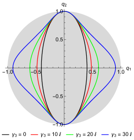
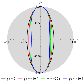
Figure 1: Plots of the real part of trajectories from the cubic perturbation of the Zernike system $\mathcal{H}_{3}$ (5.4) with $\kappa=+1$.

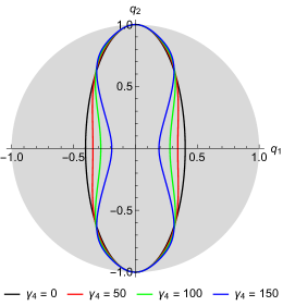
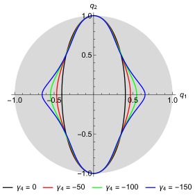
Figure 2: Plots of the real part of trajectories from the quartic perturbation of the Zernike system $\mathcal{H}_{4}$ (5.6) with $\kappa=+1$.

From the expression (3.32) one can easily check that central potential $\mathcal{U}_{\kappa}(\rho)$ with $\gamma_{1}$ given by (5.1) and with a single parameter $\gamma_{N}\neq 0$ ($N\geq 3$) is a real potential according to the parity of $N$: $\gamma_{N}$ must be a pure imaginary number when $N$ is odd, while $\gamma_{N}\in\mathbb{R}$ when $N$ is even. For these cases, it can be obtained that the real part of the trajectory is bounded. We illustrate this fact by drawing the fifth-order perturbation of the Zernike system in Fig. 3 and the sixth-order perturbation in Fig. 4 with $\kappa=+1$ and again in the projective plane $(q_{1},q_{2})$.

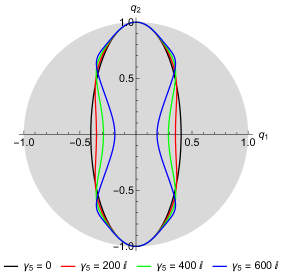
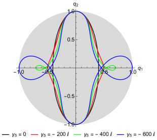
Figure 3: Plots of the real part of trajectories from the fifth-order perturbation of the Zernike system obtained from $\mathcal{H}_{5}$ (3.5) under the identification (5.1) with $\kappa=+1$ and with a single term $\gamma_{5}\neq 0$.

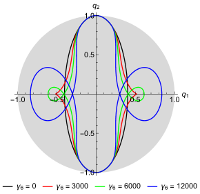
Figure 4: Plots of the real part of trajectories from the sixth-order perturbation of the Zernike system obtained from $\mathcal{H}_{6}$ (3.5) under the identification (5.1) with $\kappa=+1$ and with a single term $\gamma_{6}\neq 0$.

The superintegrable properties for the four particular perturbations of the Zernike system here considered can be extracted straightforwardly from the general results presented in Table 2 since this covers the cases with $N\leq 6$. Obviously, one can always construct superpositions of different higher-order perturbations of the Zernike system.

6 Conclusions and outlook

Throughout this work we have constructed a new class of higher-order superintegrable momentum-dependent Hamiltonians summarized in Theorem 2, which allows for an arbitrary superposition of potentials beyond the linear and quadratic momentum-dependent ones. Moreover, these systems have not only been interpreted on the 2D Euclidean plane $\mathbf{E}^{2}$ but also on the sphere $\mathbf{S}^{2}$ and the hyperbolic plane $\mathbf{H}^{2}$ in Proposition 3. The corresponding higher-order momentum-dependent constants of the motion have been explicitly written and some algebraic properties have also been studied, such as the relationship among the constants of the motion in Proposition 2 and the symmetry algebra of the integrals in Section 4.

It is worth recalling that the cornerstone of our construction is based in the superintegrable classical Zernike system [33] described in Theorem 1 together with its underlying Poisson $\mathfrak{sl}(2,\mathbb{R})$-coalgebra symmetry, presented in Section 2.2, which holds for $\mathcal{H}_{N}$ (2.31) for any $N$. From the latter property, four open problems naturally arise which could be faced in order to generalize $\mathcal{H}_{N}$ and the results of Theorem 2:

• If we consider arbitrary real parameters $\lambda_{i}$ $(i=1,2)$ in the symplectic realization (2.27), we obtain a new integrable Hamiltonian $\mathcal{H}_{\lambda,N}$ generalizing the superintegrable $\mathcal{H}_{N}$ (2.31) via a superposition with a potential $\mathcal{W}_{\lambda}(q_{1},q_{2})$ as

  $$\mathcal{H}_{\lambda,N}=\mathcal{H}_{N}+\mathcal{W}_{\lambda}(q_{1},q_{2})=\mathbf{p}^{2}+\sum_{n=1}^{N}\gamma_{n}(\mathbf{q}\boldsymbol{\cdot}\mathbf{p})^{n}+\frac{\lambda_{1}}{q_{1}^{2}}+\frac{\lambda_{2}}{q_{2}^{2}}\,,$$ (6.1)

  which is always endowed with the constant of the motion given by ${C}^{(2)}$ (2.28). In $\mathbf{E}^{2}$, with $(q_{1},q_{2})$ identified with Cartesian coordinates, the $\lambda_{i}$-terms are ‘centrifugal’ (or Rosochatius–Winternitz) potentials such that they provide centrifugal barriers when both constants are positive so restricting the trajectories to some quadrants in the Euclidean plane. In geodesic polar variables (2.16) the additional potential $\mathcal{W}_{\lambda}$ becomes

  $$\mathcal{W}_{\lambda}(\rho,\phi)=\frac{\lambda_{1}}{{\rm\ \!S}^{2}_{\kappa}(\rho)\cos^{2}\phi}+\frac{\lambda_{2}}{{\rm\ \!S}^{2}_{\kappa}(\rho)\sin^{2}\phi}\,,$$ (6.2)

  which can be interpreted as two noncentral 1 : 1 isotropic curved oscillators on $\mathbf{S}^{2}$ or as centrifugal barriers on $\mathbf{H}^{2}$ when both $\lambda_{i}>0$ [43].

• The $\mathfrak{sl}(2,\mathbb{R})$-coalgebra symmetry [31, 29] directly leads to the following quasi-maximally superintegrable generalization of the Hamiltonian (2.31) in arbitrary dimension $d$:

  $$\mathcal{H}^{(d)}_{\lambda,N}=J_{+}^{(d)}+\sum_{n=1}^{N}\gamma_{n}\left(J_{3}^{(d)}\right)^{n}=\sum_{i=1}^{d}p_{i}^{2}+\sum_{n=1}^{N}\gamma_{n}\left(\sum_{i=1}^{d}q_{i}p_{i}\right)^{n}+\sum_{i=1}^{d}\frac{\lambda_{i}}{q_{i}^{2}}\,,\qquad d\geq 2,$$ (6.3)

  which, by construction, is endowed with $(2d-3)$ functionally independent ‘universal’ constants of the motion [31, 29, 45, 46] and can be further interpreted on either $\mathbf{E}^{d}$, $\mathbf{S}^{d}$ or $\mathbf{H}^{d}$.

• The Hamiltonian $\mathcal{H}^{(d)}_{\lambda,N}$ (6.3) can also be generalized to spaces of nonconstant curvature through (non-deformed) Poisson $\mathfrak{sl}(2,\mathbb{R})$-coalgebra spaces following [62] which would allow several possibilities for a generalized momentum-dependent potential.

• And, finally, the last possible generalization is to consider Poisson–Hopf algebra deformations of $\mathfrak{sl}(2,\mathbb{R})$ [29, 63, 64] which convey an additional quantum deformation parameter $q={\rm e}^{z}$ giving rise to a deformed classical Hamiltonian $\mathcal{H}^{(d)}_{z,\lambda,N}$ such that $\lim_{z\to 0}\mathcal{H}^{(d)}_{z,\lambda,N}=\mathcal{H}^{(d)}_{\lambda,N}$. In this case, the deformation parameter $z$ would determine superintegrable perturbations of the initial (underformed) Hamiltonian (6.3).

The crucial point to solve any of the above four problems is to obtain the corresponding generalized counterpart of the constant of the motion $\mathcal{I}_{N}$ (3.6), since both the coalgebra and deformed coalgebra symmetries ensure the existence of $(2d-3)$ functionally independent constants of the motion. Clearly, these tasks are by no means trivial.

In contrast to the previous (open) discussion, it might be straightforward to apply the results of Theorem 2 and Proposition 3 to the three (1+1)D Lorentzian spacetimes of constant curvature, i.e., the Minkowskian and (anti-)de Sitter spacetimes. The procedure requires to incorporate a second ‘contraction’ parameter, say $\kappa_{2}$, beyond the curvature of the space $\kappa\equiv\kappa_{1}$, depending on the speed of light $c$ as $\kappa_{2}=-1/c^{2}$ [42, 60], which could be performed by analytic continuation. Therefore, the ‘additional’ constant of the motion $\mathcal{I}_{N}$ (3.6) would formally hold but now in a Riemannian–Lorentzian form, so that no further cumbersome computations would be needed. For instance, under this approach the Zernike system written as the natural Hamiltonian given in Proposition 1 in geodesic polar variables (2.17), with $\gamma_{1}=2{\rm i}\omega$, turns out to be

$$\mathcal{H}_{{\rm Zk},\kappa_{1},\kappa_{2}}=\mathcal{T}_{\kappa_{1},\kappa_{2}}+\mathcal{U}_{\kappa_{1}}(\rho),\qquad\mathcal{T}_{\kappa_{1},\kappa_{2}}=p_{\rho}^{2}+\frac{p_{\phi}^{2}}{\kappa_{2}{\rm\ \!S}^{2}_{\kappa_{1}}(\rho)},\qquad\mathcal{U}_{\kappa_{1}}(\rho)=\omega^{2}{\rm\ \!T}^{2}_{\kappa_{1}}(\rho),$$ (6.4)

where $\mathcal{T}_{\kappa_{1},\kappa_{2}}$ is the kinetic energy on the curved space and $\mathcal{U}_{\kappa_{1}}(\rho)$ is the 1 : 1 isotropic curved oscillator. Hence, for $\kappa_{2}=+1$ $(c={\rm i})$ the results here presented for the three Riemannian spaces of constant curvature would be recovered, meanwhile for $\kappa_{2}<0$ ($c$ finite), new results concerning Lorentzian spacetimes would be obtained. We recall that the Hamiltonian (6.4) has been deeply studied in [65] in (2+1)-dimensions (see also [66] for the specific anti-de Sitter case).

To conclude, we would like to comment on what, in our opinion, is the main open problem of this work, which is precisely to obtain the quantum analogue of the superintegrable classical Hamiltonian $\mathcal{H}_{N}$ (2.31). Let us consider the usual quantum position $\hat{\mathbf{q}}$ and momenta $\hat{\mathbf{p}}$ operators, with canonical Lie brackets and differential representation given by

$$[\hat{q}_{i},\hat{p}_{j}]={\rm i}\hbar\delta_{ij},\qquad\hat{q}_{i}\psi(\mathbf{q})=q_{i}\psi(\mathbf{q}),\qquad\hat{p}_{i}\psi(\mathbf{q})=-{\rm i}\hbar\,\frac{\partial\psi(\mathbf{q})}{\partial q_{i}}\,.$$ (6.5)

From them, we quantize the two-particle symplectic realization (2.27) (with $\lambda_{i}=0)$ in the form

$$\hat{J}_{-}^{(2)}=\hat{q}_{1}^{2}+\hat{q}_{2}^{2}\equiv\hat{\mathbf{q}}^{2},\qquad\hat{J}_{+}^{(2)}=\hat{p}_{1}^{2}+\hat{p}_{2}^{2}\equiv\hat{\mathbf{p}}^{2},\qquad\hat{J}_{3}^{(2)}=\hat{q}_{1}\hat{p}_{1}+\hat{q}_{2}\hat{p}_{2}\equiv\hat{\mathbf{q}}\boldsymbol{\cdot}\hat{\mathbf{p}}\,.$$ (6.6)

These operators close on a Lie algebra isomorphic to $\mathfrak{gl}(2)$:

$$\bigl{[}\hat{J}_{3}^{(2)},\hat{J}_{\pm}^{(2)}\bigr{]}=\pm 2{\rm i}\hbar\hat{J}_{\pm}^{(2)},\qquad\bigl{[}\hat{J}_{-}^{(2)},\hat{J}_{+}^{(2)}\bigr{]}=4{\rm i}\hbar\hat{J}_{3}^{(2)}+4\hbar^{2}{\rm Id},$$ (6.7)

where ${\rm Id}$ is the identity operator. Then we propose that the quantization of $\mathcal{H}_{N}$ (2.31) is defined by the following quantum Hamiltonian

$$\hat{\mathcal{H}}_{N}=\hat{J}_{+}^{(2)}+\sum_{n=1}^{N}\gamma_{n}\left(\hat{J}_{3}^{(2)}\right)^{n}=\hat{\mathbf{p}}^{2}+\sum_{n=1}^{N}\gamma_{n}(\hat{\mathbf{q}}\boldsymbol{\cdot}\hat{\mathbf{p}})^{n},$$ (6.8)

that is,

$$\hat{\mathcal{H}}_{N}\psi(\mathbf{q})=-\hbar^{2}\left(\frac{\partial^{2}\psi(\mathbf{q})}{\partial q_{1}^{2}}+\frac{\partial^{2}\psi(\mathbf{q})}{\partial q_{2}^{2}}\right)+\sum_{n=1}^{N}\gamma_{n}(-{\rm i}\hbar)^{n}\left(q_{1}\frac{\partial}{\partial q_{1}}+q_{2}\frac{\partial}{\partial q_{2}~{}}\right)^{n}\psi(\mathbf{q})\,.$$ (6.9)

Thus $\hat{\mathcal{H}}_{N}$ is now endowed with a Lie $\mathfrak{gl}(2)$-coalgebra symmetry (instead of a Poisson $\mathfrak{sl}(2,\mathbb{R})$-coalgebra one). We stress that such a ‘direct’ quantization does not work on the constant of the motion $\mathcal{I}_{N}$ (3.6) since serious ordering problems arise, so that additional terms must be added in order to obtain the quantum analogue of $\mathcal{I}_{N}$ and thus proving quantum superintegrability of (6.8).

Work on the above research lines is currently in progress.

References

• [1]
• [2] J. Hietarinta. New integrable Hamiltonians with transcendental invariants. Phys. Rev. Lett. 52:1057–1060, 1984. doi.org/10.1103/PhysRevLett.52.1057
• [3] J. Hietarinta. How to construct integrable Fokker–Planck and electromagnetic Hamiltonians from ordinary integrable Hamiltonians. J Math. Phys. 26:1970–1975, 1985. 10.1063/1.526865
• [4] J. M. F. Gunn. An occurrence of an effective anharmonic velocity dependent potential. J. Phys. A: Math. Gen. 18:1959–1969, 1985. doi.org/10.1088/0305-4470/18/11/020
• [5] B. Dorizzi, B. Grammaticos, A. Ramani, and P. Winternitz. Integrable Hamiltonian systems with velocity-dependent potentials. J. Math. Phys. 26:3070–3079, 1985. doi.org/10.1063/1.526685
• [6] S. Ichtiaroglou and G. Voyatzis. Integrable potentials with logarithmic integrals of motion. J. Phys. A: Math. Gen. 21:3537–3546, 1988. 110.1088/0305-4470/21/18/010
• [7] E. McSween and P. Winternitz. Integrable and superintegrable Hamiltonian systems in magnetic fields. J. Math. Phys. 41:2957–2967, 2000. doi.org/10.1063/1.533283
• [8] J. F. Cariñena, J. Fernández-Núñez, and M. F. Rañada. Singular Lagrangians affine in velocities. J. Phys. A: Math. Gen. 36:3789–3808, 2003. doi:10.1088/0305-4470/36/13/311
• [9] G. Puccaco. On integrable Hamiltonians with velocity dependent potentials. Celestial Mech. Dyn. Astr. 90:109–123, 2004. doi.org/10.1007/s10569-004-1586-y
• [10] M. F. Rañada. A system of $n=3$ coupled oscillators with magnetic terms: Symmetries and integrals of motion. SIGMA Symmetry Integrability Geom. Methods Appl. 1:004, 2005. doi.org/10.3842/SIGMA.2005.004
• [11] G. A. Moreno and R. O. Barrachina. A velocity-dependent potential of a rigid body in a rotating frame. Am. J. Phys. 76:1146–1149, 2008. doi.org/10.1119/1.2982632
• [12] A. P. Sozonov and A. V. Tsiganov. Bäcklund transformations relating different Hamilton-Jacobi equations. Theor. Math. Phys. 183:768–781, 2015. 10.1007/s11232-015-0295-x
• [13] A. V. Tsiganov. On the Chaplygin system on the sphere with velocity dependent potential. J. Geom. Phys. 92:94–99, 2015. 10.1016/j.geomphys.2015.02.006
• [14] H. M. Yehia and A. A. Elmandouh. Integrable 2D time-irreversible systems with a cubic second integral. Adv. Math. Phys. 2016:8958747, 2016. 10.1155/2016/8958747
• [15] S. Bertrand, O. Kubů, and L. $\breve{\text{S}}$nobl. On superintegrability of 3D axially-symmetric non-subgroup-type systems with magnetic fields. J. Phys. A: Math. Theor. 54:015201, 2020. doi.org/10.1088/1751-8121/abc4b8
• [16] F. Fournier, L. $\breve{\text{S}}$nobl, and P. Winternitz. Cylindrical type integrable classical systems in a magnetic field. J. Phys. A: Math. Theor. 53:085203, 2020. 10.1088/1751-8121/ab64a6
• [17] M. Razavy, G. Field, and J. S. Levinger. Analytical solutions for velocity-dependent nuclear potentials. Phys. Rev. 125:269–272, 1962. doi.org/10.1103/PhysRev.125.269
• [18] B. H. J. McKellar and R. M. May. Theory of low energy scattering by velocity dependent potentials. Nucl. Phys. 65:289–293, 1965. doi.org/10.1016/0029-5582(65)90269-5
• [19] E. M. Ferreira, N. Guillén, and J. Sesma. Properties of velocity-dependent potentials. J. Math. Phys. 8:2243–2249, 1967. doi.org/10.1063/1.1705149
• [20] J. Sesma and V. Vento. Optical analysis of resonances in a velocity-dependent potential. J. Math. Phys. 19:1293–1299, 1978. doi.org/10.1063/1.523826
• [21] A. Soylu, O. Bayrak, and I. Boztosun. Effect of the velocity-dependent potentials on the energy eigenvalues of the Morse potential. Cent. Eur. J. Phys. 10:953–959, 2012. 10.2478/s11534-012-0018-y
• [22] C. Dorso, S. Duarte, and J. Randrup. Classical simulation of the Fermi gas. Phys. Lett. B 188:287–294, 1987. doi:10.1016/0370-2693(87)91382-7
• [23] D. H. Boal and J. N. Glosli. Quasiparticle model for nuclear dynamics studies: Ground-state properties. Phys. Rev. C 38:1870–1878, 1988. doi:10.1103/PhysRevC.38.1870
• [24] P. Cordero and E. S. Hernández. Momentum-dependent potentials: Towards the molecular dynamics of fermionlike classical particles. Phys. Rev. E 51:2573–2580, 1995. doi:10.1103/PhysRevE.51.2573
• [25] J. Y. Liu, W. J. Guo, Y. Z. Xing, W. Zou, and X. G. Lee. Influence of a momentum dependent interaction on the isospin dependence of fragmentation and dissipation in intermediate energy heavy ion collisions. Phys. Rev. C 67:024608, 2003. doi:10.1103/PhysRevC.67.024608
• [26] Y. Nara, T. Maruyama, and H. Stoecker. Momentum-dependent potential and collective flows within the relativistic quantum molecular dynamics approach based on relativistic mean-field theory. Phys. Rev. C 102:024913, 2020. doi:10.1103/PhysRevC.102.024913
• [27] V. Chari and A. Pressley. A guide to Quantum Groups. Cambridge University Press, Cambridge, 1994.
• [28] A. Ballesteros and O. Ragnisco. A systematic construction of completely integrable Hamiltonians from coalgebras. J. Phys. A: Math. Gen. 31:3791–3813, 1998. doi:10.1088/0305-4470/31/16/009
• [29] A. Ballesteros, A. Blasco, F. J. Herranz, F. Musso, and O Ragnisco. (Super)integrability from coalgebra symmetry: formalism and applications. J. Phys.: Conf. Ser. 175:012004, 2009. doi:10.1088/1742-6596/175/1/012004
• [30] A. Ballesteros, E. Celeghini, and F. J. Herranz. Quantum (1+1) extended Galilei algebras: from Lie bialgebras to quantum $R$-matrices and integrable systems. J. Phys. A: Math. Gen. 33:3431–3444, 2000. doi:10.1088/0305-4470/33/17/303
• [31] A. Ballesteros and F. J. Herranz. Universal integrals for superintegrable systems on $N$-dimensional spaces of constant curvature. J. Phys. A: Math. Theor. 40:F51–F59, 2007. doi:10.1088/1751-8113/40/2/F01
• [32] A. Ballesteros, A. Blasco, and F. J. Herranz. $N$-dimensional integrability from two-photon coalgebra symmetry. J. Phys. A: Math. Theor. 42:265205, 2009. doi:10.1088/1751-8113/42/26/265205
• [33] G. S. Pogosyan, K. B. Wolf, and A. Yakhno. Superintegrable classical Zernike system. J. Math. Phys. 58:072901, 2017. doi:10.1063/1.4990793
• [34] A. P. Fordy. Classical and quantum super-integrability: From Lissajous figures to exact solvability. Phys. Atom. Nuclei 81:832–842, 2018. doi:10.1134/S1063778818060133
• [35] K. B. Wolf. From free motion on a 3-sphere to the Zernike system of wavefronts inside a circular pupil. J. Phys. Conf. Ser. 1540:012011, 2020. doi:10.1088/1742-6596/1540/1/012011
• [36] v. F. Zernike. Beugungstheorie des schneidenver-fahrens und seiner verbesserten form, der phasenkontrastmethode. Physica 1:689–704, 1934. doi:10.1016/S0031-8914(34)80259-5
• [37] G. S. Pogosyan, C. Salto-Alegre, K. B. Wolf, and A. Yakhno. Quantum superintegrable Zernike system. J. Math. Phys. 58:072101, 2017. doi:10.1063/1.4990794
• [38] N. M. Atakishiyev, G. S. Pogosyan, K. B. Wolf, and A. Yakhno. Interbasis expansions in the Zernike system. J. Math. Phys. 58:103505, 2017. doi:10.1063/1.5000915
• [39] G. S. Pogosyan, K. B. Wolf, and A. Yakhno. New separated polynomial solutions to the Zernike system on the unit disk and interbasis expansion. J. Opt. Soc. Am. A 34:1844–1848, 2017. doi:10.1364/josaa.34.001844
• [40] N. M. Atakishiyev, G. S. Pogosyan, K. B. Wolf, and A. Yakhno. Spherical geometry, Zernike’s separability, and interbasis expansion coefficients. J. Math. Phys. 60:101701, 2019. doi:10.1063/1.5099974
• [41] M. F. Rañada and M. Santander. Superintegrable systems on the two-dimensional sphere $S^{2}$ and the hyperbolic plane $H^{2}$. J. Math. Phys. 40:5026–5057, 1999. doi:10.1063/1.533014
• [42] F. J.  Herranz and M. Santander. Conformal symmetries of spacetimes. J. Phys. A: Math. Gen. 35:6601–6618, 2002. doi:10.1088/0305-4470/35/31/306
• [43] A. Ballesteros, F. J. Herranz, and F. Musso. The anisotropic oscillator on the 2D sphere and the hyperbolic plane. Nonlinearity 26:971–990, 2013. doi:10.1088/0951-7715/26/4/971
• [44] P. W. Higgs. Dynamical symmetries in a spherical geometry I. J. Phys. A: Math. Gen. 12:309–323, 1979. doi:10.1088/0305-4470/12/3/006
• [45] D. Latini. Universal chain structure of quadratic algebras for superintegrable systems with coalgebra symmetry. J. Phys. A: Math. Theor. 52:125202, 2019. doi:10.1088/1751-8121/aaffec
• [46] D. Latini, I. Marquette, and Y.-Z. Zhang. Racah algebra $R(n)$ from coalgebraic structures and chains of $R(3)$ substructures. J. Phys. A: Math. Theor. 54:395202, 2021. doi:10.1088/1751-8121/ac1ee8
• [47] A. M. Perelomov. Integrable systems of classical mechanics and Lie algebras. Birkhäuser, Berlin, 1990.
• [48] H. I. Leemon. Dynamical symmetries in a spherical geometry II. J. Phys. A: Math. Gen. 12:489–501,1979. doi:10.1088/0305-4470/12/4/009
• [49] Ye. M. Hakobyan, G. S. Pogosyan, A. N. Sissakian, and S. I. Vinitsky. Isotropic oscillator in a space of constant positive curvature: Interbasis expansions. Phys. Atom. Nucl. 62:623–637, 1999. arXiv:quant-ph/9710045
• [50] E. G. Kalnins, G. S. Pogosyan, and W. Jr. Miller. Completeness of multiseparable superintegrability on the complex 2-sphere. J. Phys. A: Math. Gen. 33:6791–6806, 2000. doi:10.1088/0305-4470/33/38/310
• [51] E. G. Kalnins, J. M. Kress, G. S. Pogosyan, and W. Jr. Miller. Completeness of superintegrability in two-dimensional constant-curvature spaces. J. Phys. A: Math. Gen. 34:4705–4720, 2001. doi:10.1088/0305-4470/34/22/311
• [52] A. Nersessian and G. Pogosyan. Relation of the oscillator and Coulomb systems on spheres and pseudospheres. Phys. Rev. A 63:020103, 2001. doi:10.1103/PhysRevA.63.020103
• [53] J. F. Cariñena, M. F. Rañada, M. Santander, and M. Senthilvelan. A non-linear oscillator with quasi-harmonic behaviour: two- and n-dimensional oscillators. Nonlinearity 17:1941–1963, 2004. doi:10.1088/0951-7715/17/5/019
• [54] J. F. Cariñena, M. F. Rañada, and M. Santander. The quantum harmonic oscillator on the sphere and the hyperbolic plane. Ann. Phys. 322:2249–2278, 2007. doi:10.1016/j.aop.2006.10.010
• [55] W. Jr. Miller, S. Post, and P. Winternitz. Classical and quantum superintegrability with applications. J. Phys. A: Math. Theor. 46:423001, 2013. doi:10.1088/1751-8113/46/42/423001
• [56] C. Gonera and M. Kaszubska. Superintegrable systems on spaces of constant curvature. Ann. Phys. 364:91–102, 2014. doi:10.1016/j.aop.2014.04.005
• [57] A. Ballesteros, A. Blasco, F. J. Herranz, and F. Musso. A new integrable anisotropic oscillator on the two-dimensional sphere and the hyperbolic plane. J. Phys. A: Math. Theor. 47:345204, 2014. doi:10.1088/1751-8113/47/34/345204
• [58] A. Ballesteros, F. J. Herranz, S. Kuru, and J. Negro. The anisotropic oscillator on curved spaces: A new exactly solvable model. Ann. Phys. 373:399–423, 2016. doi:10.1016/j.aop.2016.07.006
• [59] A. Ballesteros and F. J. Herranz. Maximal superintegrability of the generalized Kepler–Coulomb system on N-dimensional curved spaces. J. Phys. A: Math. Theor. 42:245203, 2009. doi:10.1088/1751-8113/42/24/245203
• [60] F. J.  Herranz R. Ortega, and M. Santander. Trigonometry of spacetimes: A new self-dual approach to a curvature/signature (in)dependent trigonometry. J. Phys. A: Math. Gen. 33:4525–4551, 2000. doi:10.1088/0305-4470/33/24/309
• [61] A. Ballesteros, A. Enciso, F. J. Herranz, and O Ragnisco. Superintegrable anharmonic oscillators on $N$-dimensional curved spaces. J. Nonlinear Math. Phys. 15 suppl. 3:43-52, 2008. doi:10.2991/jnmp.2008.15.s3.5
• [62] A. Ballesteros, A. Enciso, F. J. Herranz, and O. Ragnisco. $N$-dimensional $sl(2)$-coalgebra spaces with non-constant curvature. Phys. Lett. B 652:376–383, 2007. doi:10.1016/j.physletb.2007.07.012
• [63] A. Ballesteros, F. J. Herranz, and O. Ragnisco. Integrable potentials on spaces with curvature from quantum groups. J. Phys. A: Math. Gen. 38:7129–7144, 2005. doi:10.1088/0305-4470/38/32/004
• [64] O. Ragnisco, A. Ballesteros, F. J. Herranz, and F. Musso. Quantum deformations and superintegrable motions on spaces with variable curvature. SIGMA Symmetry Integrability Geom. Methods Appl. 3:026, 2007. doi:10.3842/SIGMA.2007.026
• [65] F. J. Herranz and A. Ballesteros. Superintegrability on three-dimensional Riemannian and relativistic spaces of constant curvature. SIGMA Symmetry Integrability Geom. Methods Appl. 2:010, 2006. doi:10.3842/SIGMA.2006.010
• [66] D. R. Petrosyan and G. S. Pogosyan. Harmonic oscillator on the $SO(2,2)$ hyperboloid. SIGMA Symmetry Integrability Geom. Methods Appl. 11:096, 2015. doi:10.3842/SIGMA.2015.096