p-Meta: Towards On-device Deep Model Adaptation

Abstract.

Data collected by IoT devices are often private and have a large diversity across users. Therefore, learning requires pre-training a model with available representative data samples, deploying the pre-trained model on IoT devices, and adapting the deployed model on the device with local data. Such an on-device adaption for deep learning empowered applications demands data and memory efficiency. However, existing gradient-based meta learning schemes fail to support memory-efficient adaptation. To this end, we propose p-Meta, a new meta learning method that enforces structure-wise partial parameter updates while ensuring fast generalization to unseen tasks. Evaluations on few-shot image classification and reinforcement learning tasks show that p-Meta not only improves the accuracy but also substantially reduces the peak dynamic memory by a factor of 2.5 on average compared to state-of-the-art few-shot adaptation methods.

1. Introduction

Adaption to unseen environments, users, and tasks is crucial for deep learning empowered IoT applications to deliver consistent performance and customized services. Data collected by IoT devices are often private and have a large diversity across users. For instance, activity recognition with smartphone sensors should adapt to countless walking patterns and sensor orientation (Gong et al., 2019). Human motion prediction with home robots needs fast learning of unseen poses for seamless human-robot interaction (Gui et al., 2018). In these applications, the new data collected for model adaptation tend to relate to personal habits and lifestyle. Hence, on-device model adaptation is preferred over uploading the data to cloud servers for retraining.

Yet on-device adaption of a deep neural network (DNN) demands data efficiency and memory efficiency. The excellent accuracy of contemporary DNNs is attributed to training with high-performance computers on large-scale datasets (Goodfellow et al., 2016). For example, it takes $29$ hours to complete a $90$-epoch ResNet50 (He et al., 2016) training on ImageNet ($1.2$ million training images) (Russakovsky et al., 2015) with $8$ NVIDIA Tesla P100 GPUs (Goyal et al., 2017). For on-device adaptation, however, neither abundant data nor resources are available. A personal voice assistant, for example, may learn to adapt to users’ accent and dialect within a few sentences, while a home robot should learn to recognize new object categories with few labelled images to navigate in new environments. Furthermore, such adaptation is expected to be conducted on low-resource platforms such as smart portable devices, home hubs, and other IoT devices, with only several $KB$ to $MB$ memory.

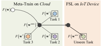
Figure 1. Meta learning and few-shot learning (FSL) in the context of on-device adaptation. The backbone $F(\bm{w})$ is meta-trained into $F(\bm{w}^{\mathrm{meta}})$ on the cloud and is deployed to IoT devices to adapt to unseen tasks as $F(\bm{w}^{\mathrm{new}})$ via FSL.

For data-efficient DNN adaptation, we resort to meta learning, a paradigm that learns to fast generalize to unseen tasks (Hospedales et al., 2020). Of our particular interest is gradient-based meta learning (Antoniou et al., 2019; Finn et al., 2017; Raghu et al., 2020; Oh et al., 2021) for its wide applicability in classification, regression and reinforcement learning, as well as the availability of gradient-based training frameworks for low-resource devices, e.g., TensorFlow Lite (TensorFlow, [n.d.]). Fig. 1 explains major terminologies in the context of on-device adaptation. Given a backbone, its weights are meta-trained on many tasks, to output a model that is expected to fast adapt to new unseen tasks. The process of adaptation is also known as few-shot learning, where the meta-trained model is further retrained by standard stochastic gradient decent (SGD) on few new samples only.

However, existing gradient-based meta learning schemes (Antoniou et al., 2019; Finn et al., 2017; Raghu et al., 2020; Oh et al., 2021) fail to support memory-efficient adaptation. Although meta training is conducted in the cloud, few-shot learning (adaptation) of the meta-trained model is performed on IoT devices. Consider to retrain a common backbone ResNet12 in a 5-way (5 new classes) 5-shot (5 samples per class) scenario. One round of SGD consumes 370.44MB peak dynamic memory, since the inputs of all layers must be stored to compute the gradients of these layers’ weights in the backward path. In comparison, inference only needs 3.61MB. The necessary dynamic memory is a key bottleneck for on-device adaptation due to cost and power constraints, even though the meta-trained model only needs to be retrained with a few data.

Prior efficient DNN training solutions mainly focus on parallel and distributed training on data centers (Chen et al., 2016; Chen et al., 2021; Greff et al., 2017; Gruslys et al., 2016; Raihan and Aamodt, 2020). On-device training has been explored for vanilla supervised training (Gooneratne et al., 2020; Mathur et al., 2021; Lee and Nirjon, 2019), where training and testing are performed on the same task. A pioneer study (Cai et al., 2020) investigated on-device adaptation to new tasks via memory-efficient transfer learning. Yet transfer learning is prone to overfitting when only a few samples are available (Finn et al., 2017).

In this paper, we propose p-Meta, a new meta learning method for data- and memory-efficient DNN adaptation. The key idea is to enforce structured partial parameter updates while ensuring fast generalization to unseen tasks. The idea is inspired by recent advances in understanding gradient-based meta learning (Oh et al., 2021; Raghu et al., 2020). Empirical evidence shows that only the head (the last output layer) of a DNN needs to be updated to achieve reasonable few-shot classification accuracy (Raghu et al., 2020) whereas the body (the layers closed to the input) needs to be updated for cross-domain few-shot classification (Oh et al., 2021). These studies imply that certain weights are more important than others when generalizing to unseen tasks. Hence, we propose to automatically identify these adaptation-critical weights to minimize the memory demand in few-shot learning.

Particularly, the critical weights are determined in two structured dimensionalities as, (i) layer-wise: we meta-train a layer-by-layer learning rate that enables a static selection of critical layers for updating; (ii) channel-wise: we introduce meta attention modules in each layer to select critical channels dynamically, i.e., depending on samples from new tasks. Partial updating of weights means that (structurally) sparse gradients are generated, reducing memory requirements to those for computing nonzero gradients. In addition, the computation demand for calculating zero gradients can be also saved. To further reduce the memory, we utilize gradient accumulation in few-shot learning and group normalization in the backbone. Although weight importance metrics and SGD with sparse gradients have been explored in vanilla training (Raihan and Aamodt, 2020; Deng et al., 2020; Gooneratne et al., 2020; Han et al., 2016), it is unknown (i) how to identify adaptation-critical weights and (ii) whether meta learning is robust to sparse gradients, where the objective is fast adaptation to unseen tasks.

Our main contributions are summarized as follows.

• We design p-Meta, a new meta learning method for data- and memory-efficient DNN adaptation to unseen tasks. p-Meta automatically identifies adaptation-critical weights both layer-wise and channel-wise for low-memory adaptation. The hierarchical approach combines static identification of layers and dynamic identification of channels whose weights are critical for few-shot adaptation. To the best of our knowledge, p-Meta is the first meta learning method designed for on-device few-shot learning.

• Evaluations on few-shot image classification and reinforcement learning show that, p-Meta not only improves the accuracy but also reduces the peak dynamic memory by a factor of 2.5 on average over the state-of-the-art few-shot adaptation methods. p-Meta can also simultaneously reduce the computation by a factor of 1.7 on average.

In the rest of this paper, we introduce the preliminaries and challenges in Sec. 2, elaborate on the design of p-Meta in Sec. 3, present its evaluations in Sec. 4, review related work in Sec. 5, and conclude in Sec. 6.

2. Preliminaries and Challenges

In this section, we provide the basics on meta learning for fast adaptation and highlight the challenges to enable on-device adaptation.

Meta Learning for Fast Adaptation. Meta learning is a prevailing solution to adapt a DNN to unseen tasks with limited training samples, i.e., few-shot learning (Hospedales et al., 2020). We ground our work on model-agnostic meta learning (MAML) (Finn et al., 2017), a generic meta learning framework which supports classification, regression and reinforcement learning. Given the dataset $\mathcal{D}=\{\mathcal{S},\mathcal{Q}\}$ of an unseen few-shot task, where $\mathcal{S}$ (support set) and $\mathcal{Q}$ (query set) are for training and testing, MAML trains a model $F(\bm{w})$ with weights $\bm{w}$ such that it yields high accuracy on $\mathcal{Q}$ even when $\mathcal{S}$ only contains a few samples. This is enabled by simulating the few-shot learning experiences over abundant few-shot tasks sampled from a task distribution $p(\mathsf{T})$. Specifically, it meta-trains a backbone $F$ over few-shot tasks $\mathsf{T}^{i}\sim p(\mathsf{T})$, where each $\mathsf{T}^{i}$ has dataset $\mathcal{D}^{i}=\{\mathcal{S}^{i},\mathcal{Q}^{i}\}$, and then generates $F(\bm{w}^{\mathrm{meta}})$, an initialization for the unseen few-shot task $\mathsf{T}^{\mathrm{new}}$ with dataset $\mathcal{D}^{\mathrm{new}}=\{\mathcal{S}^{\mathrm{new}},\mathcal{Q}^{\mathrm{new}}\}$. Training from $F(\bm{w}^{\mathrm{meta}})$ over $\mathcal{S}^{\mathrm{new}}$ is expected to achieve a high test accuracy on $\mathcal{Q}^{\mathrm{new}}$.

MAML achieves fast adaptation via two-tier optimization. In the inner loop, a task $\mathsf{T}^{i}$ and its dataset $\mathcal{D}^{i}$ are sampled. The weights $\bm{w}$ are updated to $\bm{w}^{i}$ on support dataset $\mathcal{S}^{i}$ via $K$ gradient descent steps, where $K$ is usually small, compared to vanilla training:

(1) $$\medop{\bm{w}^{i,k}=\bm{w}^{i,k-1}-\alpha\nabla_{\bm{w}}~{}\ell\left(\bm{w}^{i,k-1};\mathcal{S}^{i}\right)\quad\mathrm{for}~{}k=1\cdots K}$$

where $\bm{w}^{i,k}$ are the weights at step $k$ in the inner loop, and $\alpha$ is the inner step size. Note that $\bm{w}^{i,0}=\bm{w}$ and $\bm{w}^{i}=\bm{w}^{i,K}$. $\ell(\bm{w};\mathcal{D})$ is the loss function on dataset $\mathcal{D}$. In the outer loop, the weights are optimized to minimize the sum of loss at $\bm{w}^{i}$ on query dataset $\mathcal{Q}^{i}$ across tasks. The gradients to update weights in the outer loop are calculated w.r.t. the starting point $\bm{w}$ of the inner loop.

(2) $$\medop{\bm{w}\leftarrow\bm{w}-\beta\nabla_{\bm{w}}\sum_{i}\ell\left(\bm{w}^{i};\mathcal{Q}^{i}\right)}$$

where $\beta$ is the outer step size.

Table 1. The static memory, the peak dynamic memory, and the total computation (GMACs $=10^{9}$MACs) of inference and adaptation for sample applications. For image classification we use batch size $=25$. For robot locomotion we use rollouts $=20$, horizon $=200$; each sample corresponds to a rollouted episode, and the case for an observation is reported in brackets. The calculation is based on Appendix A.

Application	Model / Benchmark	Static Memory (MB)		Peak Dynamic Memory (MB)		GMACs
		Model	Sample	Inference	Adaptation	Inference	Adaptation
Image Classification	4Conv (Finn et al., 2017) / MiniImageNet (Vinyals et al., 2016)	$0.13$	$0.53$	$0.90$	$48.33$	$0.72$	$1.96$
Image Classification	ResNet12 (Oreshkin et al., 2018) / MiniImageNet (Vinyals et al., 2016)	$32.0$	$0.53$	$3.61$	$370.44$	$62.08$	$185.42$
Robot Locomotion	MLP (Finn et al., 2017) / MuJoCo (Todorov et al., 2012)	$0.05$	$0.016(0.00008)$	$0.08(0.0004)$	$3.72$	$0.05$	$0.15$

The meta-trained weights $\bm{w}^{\mathrm{meta}}$ are then used as initialization for few-shot learning into $\bm{w}^{\mathrm{new}}$ by $K$ gradient descent steps over $\mathcal{S}^{\mathrm{new}}$. Finally we assess the accuracy of $F(\bm{w}^{\mathrm{new}})$ on $\mathcal{Q}^{\mathrm{new}}$.

Memory Bottleneck of On-device Adaptation. As mentioned above, the meta-trained model $F(\bm{w}^{\mathrm{meta}})$ can adapt to unseen tasks via $K$ gradient descent steps. Each step is the same as the inner loop of meta-training Eq.(1), but on dataset $\mathcal{S}^{\mathrm{new}}$.

(3) $$\medop{\bm{w}^{\mathrm{new},k}=\bm{w}^{\mathrm{new},k-1}-\alpha\nabla_{\bm{w}^{\mathrm{new}}}~{}\ell\left(\bm{w}^{\mathrm{new},k-1};\mathcal{S}^{\mathrm{new}}\right)}$$

where $\bm{w}^{\mathrm{new},0}=\bm{w}^{\mathrm{meta}}$. For brevity, we omit the superscripts of model adaption in Eq.(3) and use $\bm{g}(\cdot)$ as the loss gradients w.r.t. the given tensor. Hence, without ambiguity, we simplify the notations of Eq.(3) as follows:

(4) $$\medop{\bm{w}\leftarrow\bm{w}-\alpha\bm{g}(\bm{w})}$$

Let us now understand where the main memory cost for iterating Eq.(4) comes from. For the sake of clarity, we focus on a feed forward DNNs that consist of $L$ convolutional (conv) layers or fully-connected (fc) layers. A typical layer (see Fig. 2) consists of two operations: (i) a linear operation with trainable parameters, e.g., convolution or affine; (ii) a parameter-free non-linear operation (may not exist in certain layers), where we consider max-pooling or ReLU-styled (ReLU, LeakyReLU) activation functions in this paper.

Figure 2. A typical layer $l$ in DNNs. $\bm{x}_{l-1}$ is the input tensor; $\bm{x}_{l}$ is the output tensor, also the input tensor of layer $l+1$; $\bm{y}_{l}$ is the intermediate tensor; $\bm{w}_{l}$ is the weight tensor.

Take a network consisting of conv layers only as an example. The memory requirements for storing the activations $\bm{x}_{l}\in\mathbb{R}^{C_{l}\times H_{l}\times W_{l}}$ as well as the convolution weights $\bm{w}_{l}\in\mathbb{R}^{C_{l}\times C_{l-1}\times S_{l}\times S_{l}}$ of layer $l$ in words can be determined as

$$\medop{m(\bm{x}_{l})=C_{l}H_{l}W_{l}\;,\;\;m(\bm{w}_{l})=C_{l}C_{l-1}S_{l}^{2}}$$

where $C_{l-1}$, $C_{l}$, $H_{l}$, and $W_{l}$ stand for input channel number, output channel number, height and width of layer $l$, respectively; $S_{l}$ stands for the kernel size. The detailed memory and computation demand analysis as provided in Appendix A reveals that the by far largest memory requirement is neither attributed to determining the activations $\bm{x}_{l}$ in the forward path nor to determining the gradients of the activations $\bm{g}(\bm{x}_{l})$ in the backward path. Instead, the memory bottleneck lies in the computation of the weight gradients $\bm{g}(\bm{w}_{l})$, which requires the availability of the activations $\bm{x}_{l-1}$ from the forward path. Following Eq.(17) in Appendix A, the necessary memory in words is

(5) $$\medop{\sum_{1\leq l\leq L}m(\bm{x}_{l-1})}$$

Tab. 1 summarizes the memory consumption and the total computation of the commonly used few-shot learning backbone models (Finn et al., 2017; Oreshkin et al., 2018). The requirements are based on the detailed analysis in Appendix A. We can draw two intermediate conclusions.

• The total computation of adaptation (training) is approximately $2.7\times$ to $3\times$ larger compared to inference. Yet the peak dynamic memory of training is far larger, $47\times$ to $103\times$ over inference. The peak dynamic memory consumption of training is also also significantly higher than the static memory consumption from the model and the training samples in few-shot learning.

• To enable adaptation for memory-constrained IoT devices, we need to find some way of getting rid of the major dynamic memory contribution in Eq.(5).

3. Method

This section presents p-Meta, a new meta learning scheme that enables memory-efficient few-shot learning on unseen tasks.

3.1. p-Meta Overview

We first provide an overview of p-Meta and introduce its main concepts, namely selecting critical gradients, using a hierarchical approach to determine adaption-critical layers and channels, and using a mixture of static and dynamic selection mechanisms.

Principles. We impose structured sparsity on the gradients $\bm{g}(\bm{w}_{l})$ such that the corresponding tensor dimensions of $\bm{x}_{l}$ do not need to be saved. There are other options to reduce the dominant memory demand in Eq.(5). They are inapplicable for the reasons below.

• One may trade-off computation and memory by recomputing activations $\bm{x}_{l-1}$ when needed for determining $\bm{w}_{l}$, see for example (Chen et al., 2016; Gruslys et al., 2016). Due to the limited processing abilities of IoT devices, we exclude this option.

• It is also possible to prune activations $\bm{x}_{l-1}$. Yet based on our experiments in Appendix B.3, imposing sparsity on $\bm{x}_{l-1}$ hugely degrades few-shot learning accuracy as this causes error accumulation along the propagation, see also (Raihan and Aamodt, 2020).

• Note that unstructured sparsity, as proposed in (Gao et al., 2021; Von Oswald et al., 2021), does not in general lead to memory savings, since there is a very small probability that all weight gradients for which an element of $\bm{x}_{l-1}$ is necessary have been pruned.

We impose sparsity on the gradients in a hierarchical manner.

• Selecting adaption-critical layers. We first impose layer-by-layer sparsity on $\bm{g}(\bm{w}_{l})$. It is motivated by previous results showing that manual freezing of certain layers does no harm to few-shot learning accuracy (Raghu et al., 2020; Oh et al., 2021). Layer-wise sparsity reduces the number of layers whose weights need to be updated. We determine the adaptation-critical layers from the meta-trained layer-wise sparse learning rates.

• Selecting adaption-critical channels. We further reduce the memory demand by imposing sparsity on $\bm{g}(\bm{w}_{l})$ within each layer. Noting that calculating $\bm{g}(\bm{w}_{l})$ needs both the input channels $\bm{x}_{l-1}$ and the output channels $\bm{g}(\bm{y}_{l})$, we enforce sparsity on both of them. Input channel sparsity decreases memory and computation overhead, whereas output channel sparsity improves few-shot learning accuracy and reduces computation. We design a novel meta attention mechanism to dynamically determine adaptation-critical channels. They take as inputs $\bm{x}_{l-1}$ and $\bm{g}(\bm{y}_{l})$ and determine adaptation-critical channels during few-shot learning, based on the given few data samples from new unseen tasks. Dynamic channel-wise learning rates as determined by meta attention yield a significantly higher accuracy than a static channel-wise learning rate (see Sec. 4.4).

Memory Reduction. The reduced memory demand due to our hierarchical approach can be seen in Eq.(17) in Appendix A:

$$\medop{\sum_{1\leq l\leq L}\hat{\alpha}_{l}\mu^{\mathrm{fw}}_{l}m(\bm{x}_{l-1})}$$

where $\hat{\alpha}_{l}\in\{0,1\}$ is the mask from the static selection of critical layers and $0\leq\mu^{\mathrm{fw}}_{l}\leq 1$ denotes the relative amount of dynamically chosen input channels.

Next, we explain how p-Meta selects adaptation-critical layers (Sec. 3.2) and channels within layers (Sec. 3.3) as well as the deployment optimizations (Sec. 3.5) for memory-efficient adaptation.

3.2. Selecting Adaption-Critical Layers by Learning Sparse Inner Step Sizes

This subsection introduces how p-Meta meta-learns adaptation-critical layers to reduce the number of updated layers during few-shot learning. Particularly, instead of manual configuration as in (Oh et al., 2021; Raghu et al., 2020), we propose to automate the layer selection process. During meta training, we identify adaptation-critical layers by learning layer-wise sparse inner step sizes (Sec. 3.2.1). Only these critical layers with nonzero step sizes will be updated during on-device adaptation to new tasks (Sec. 3.2.2).

3.2.1. Learning Sparse Inner Step Sizes in Meta Training

Prior work (Antoniou et al., 2019) suggests that instead of a global fixed inner step size $\alpha$, learning the inner step sizes $\bm{\alpha}$ for each layer and each gradient descent step improves the generalization of meta learning, where $\bm{\alpha}=\alpha_{1:L}^{1:K}\succeq\bm{0}$. We utilize such learned inner step sizes to infer layer importance for adaptation. We learn the inner step sizes $\bm{\alpha}$ in the outer loop of meta-training while fixing them in the inner loop.

Learning Layer-wise Inner Step Sizes. We change the inner loop of Eq.(1) to incorporate the per-layer inner step sizes:

(6) $$\medop{\bm{w}_{l}^{i,k}=\bm{w}_{l}^{i,k-1}-\alpha^{k}_{l}\nabla_{\bm{w}_{l}}~{}\ell\left(\bm{w}^{i,k-1}_{1:L};\mathcal{S}^{i}\right)}$$

where $\bm{w}_{l}^{i,k}$ is the weights of layer $l$ at step $k$ optimized on task $i$ (dataset $\mathcal{S}^{i}$). In the outer loop, weights $\bm{w}$ are still optimized as

(7) $$\medop{\bm{w}\leftarrow\bm{w}-\beta\nabla_{\bm{w}}\sum_{i}\ell\left(\bm{w}^{i};\mathcal{Q}^{i}\right)}$$

where $\bm{w}^{i}=\bm{w}^{i,K}=\bm{w}^{i,K}_{1:L}$, which is a function of $\bm{\alpha}$. The inner step sizes $\bm{\alpha}$ are then optimized as

(8) $$\medop{\bm{\alpha}\leftarrow\bm{\alpha}-\beta\nabla_{\bm{\alpha}}\sum_{i}\ell\left(\bm{w}^{i};\mathcal{Q}^{i}\right)}$$

Imposing Sparsity on Inner Step Sizes. To facilitate layer selection, we enforce sparsity in $\bm{\alpha}$, i.e., encouraging a subset of layers to be selected for updating. Specifically, we add a Lasso regularization term in the loss function of Eq.(8) when optimizing $\bm{\alpha}$. Hence, the final optimization of $\bm{\alpha}$ in the outer loop is formulated as

(9) $$\medop{\bm{\alpha}\leftarrow\bm{\alpha}-\beta\nabla_{\bm{\alpha}}(\sum_{i}\ell\left(\bm{w}^{i};\mathcal{Q}^{i}\right)+\lambda\sum_{l,k}m(\bm{x}_{l-1})\cdot|\alpha_{l}^{k}|)}$$

where $\lambda$ is a positive scalar to control the ratio between two terms in the loss function. We empirically set $\lambda=0.001$. $|\alpha_{l}^{k}|$ is re-weighted by $m(\bm{x}_{l-1})$, which denotes the necessary memory in Eq.(5) if only updating the weights in layer $l$.

3.2.2. Exploiting Sparse Inner Step Sizes for On-device Adaptation

We now explain how to apply the learned $\bm{\alpha}$ to save memory during on-device adaptation. After deploying the meta-trained model to IoT devices for adaptation, at updating step $k$, for layers with $\alpha_{l}^{k}=0$, the activations (i.e., their inputs) $\bm{x}_{l-1}$ need not be stored, see Eq.(16) and Eq.(17) in Appendix A. In addition, we do not need to calculate the corresponding weight gradients $\bm{g}(\bm{w}_{l})$, which saves computation, see Eq.(18) in Appendix A.

3.3. Selecting Adaption-Critical Channels within Layers via Sparse Meta Attention

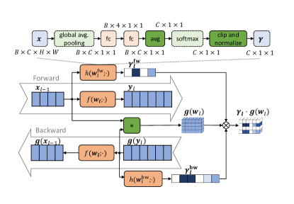
Figure 3. Meta attention of layer $l$ during meta-training. The blue blocks correspond to tensors; the orange blocks correspond to computation units with parameters, and the green ones without. Each column of a tensor corresponds to one channel. The input tensor $\bm{x}_{l-1}$ has 4 channels; the output tensor $\bm{y}_{l}$ has 6 channels. The other dimensions (e.g., height, width and batch) are omitted here. The green block with $*$ stands for the operations involved to compute $\bm{g}(\bm{w}_{l})$. In order to compute the gradients of the parameters in meta attention, i.e., $\bm{w}_{l}^{\mathrm{fw}}$ and $\bm{w}_{l}^{\mathrm{bw}}$, the full dense gradients $\bm{g}(\bm{w}_{l})$ are computed during meta-training, and then are masked by $\bm{\gamma}_{l}$. An example meta attention module for a conv layer is shown in the upper part. $B$ denotes the batch size. The newly added blocks related to the inference attention in (Chen et al., 2020) are marked with solid lines.

This subsection explains how p-Meta learns a novel meta attention mechanism in each layer to dynamically select adaptation-critical channels for further memory saving in few-shot learning. Despite the widespread adoption of channel-wise attention for inference (Hu et al., 2018; Chen et al., 2020), we make the first attempt to use attention for memory-efficient training (few-shot learning in our case). For each layer, its meta attention outputs a dynamic channel-wise sparse attention score based on the samples from new tasks. The sparse attention score is used to re-weight (also sparsify) the weight gradients. Therefore, by calculating only the nonzero gradients of critical weights within a layer, we can save both memory and computation. We first present our meta attention mechanism during meta training (Sec. 3.3.1) and then show its usage for on-device model adaptation (Sec. 3.3.2).

3.3.1. Learning Sparse Meta Attention in Meta Training

Since mainstream backbones in meta learning use small kernel sizes (1 or 3), we design the meta attention mechanism channel-wise. Fig. 3 illustrates the attention design during meta-training.

Learning Meta Attention. The attention mechanism is as follows.

• We assign an attention score to the weight gradients of layer $l$ in the inner loop of meta training. The attention scores are expected to indicate which weights/channels are important and thus should be updated in layer $l$.

• The attention score is obtained from two attention modules: one taking $\bm{x}_{l-1}$ as input in the forward pass, and the other taking $\bm{g}(\bm{y}_{l})$ as input during the backward pass. We use $\bm{x}_{l-1}$ and $\bm{g}(\bm{y}_{l})$ to calculate the attention scores because they are used to compute the weight gradients $\bm{g}(\bm{w}_{l})$.

Concretely, we define the forward and backward attention scores for a conv layer as,

(10) $$\medop{\bm{\gamma}^{\mathrm{fw}}_{l}=h(\bm{w}^{\mathrm{fw}}_{l};\bm{x}_{l-1})\in\mathbb{R}^{C_{l-1}\times 1\times 1}}$$

(11) $$\medop{\bm{\gamma}^{\mathrm{bw}}_{l}=h(\bm{w}^{\mathrm{bw}}_{l};\bm{g}(\bm{y}_{l}))\in\mathbb{R}^{C_{l}\times 1\times 1}}$$

where $h(\cdot;\cdot)$ stands for the meta attention module, and $\bm{w}^{\mathrm{fw}}_{l}$ and $\bm{w}^{\mathrm{bw}}_{l}$ are the parameters of the meta attention modules. The overall (sparse) attention scores $\bm{\gamma}_{l}\in\mathbb{R}^{C_{l}\times C_{l-1}\times 1\times 1}$ and is computed as,

(12) $$\medop{\gamma_{l,ba11}=\gamma^{\mathrm{fw}}_{l,a11}\cdot\gamma^{\mathrm{bw}}_{l,b11}}$$

In the inner loop, for layer $l$, step $k$ and task $i$, $\bm{\gamma}_{l}$ is (broadcasting) multiplied with the dense weight gradients to get the sparse ones,

(13) $$\medop{\bm{\gamma}_{l}^{i,k}\odot\nabla_{\bm{w}_{l}}~{}\ell\left(\bm{w}^{i,k-1}_{1:L};\mathcal{S}^{i}\right)}$$

The weights are then updated by,

(14) $$\medop{\bm{w}_{l}^{i,k}=\bm{w}_{l}^{i,k-1}-\alpha^{k}_{l}(\bm{\gamma}_{l}^{i,k}\odot\nabla_{\bm{w}_{l}}~{}\ell\left(\bm{w}^{i,k-1}_{1:L};\mathcal{S}^{i}\right))}$$

Let all attention parameters be $\bm{w}^{\mathrm{atten}}=\{\bm{w}^{\mathrm{fw}}_{l},\bm{w}^{\mathrm{bw}}_{l}\}_{l=1}^{L}$. The attention parameters $\bm{w}^{\mathrm{atten}}$ are optimized in the outer loop as,

(15) $$\medop{\bm{w}^{\mathrm{atten}}\leftarrow\bm{w}^{\mathrm{atten}}-\beta\nabla_{\bm{w}^{\mathrm{atten}}}\sum_{i}\ell\left(\bm{w}^{i};\mathcal{Q}^{i}\right)}$$

Note that we use a dense forward path and a dense backward path in both meta-training and on-device adaptation, as shown in Fig. 3. That is, the attention scores $\bm{\gamma}^{\mathrm{fw}}_{l}$ and $\bm{\gamma}^{\mathrm{bw}}_{l}$ are only calculated locally and will not affect $\bm{y}_{l}$ during forward and $\bm{g}(\bm{x}_{l-1})$ during backward.

Input: softmax output (normalized) $\bm{\pi}\in\mathbb{R}^{C}$, clip ratio $\rho$

Output: sparse $\bm{\gamma}$

1 Sort $\bm{\pi}$ in ascending order and get sorted indices $d_{1:C}$;

2 Find the smallest $c$ such that $\sum_{i=1}^{c}\pi_{d_{i}}\geq\rho$;

Set $\pi_{d_{1}:d_{c}}$ as 0 ;

  // if $\rho=0$, do nothing

3 Normalize $\bm{\gamma}=\bm{\pi}/\sum\bm{\pi}$;

Re-scale $\bm{\gamma}=\bm{\gamma}\cdot C$ ;

  // keeping step sizes’ magnitude

Algorithm 1 Clip and normalization

Input: meta-training task distribution $p(\mathsf{T})$, backbone $F$ with initial weights $\bm{w}$, meta attention parameters $\bm{w}^{\mathrm{atten}}$, inner step sizes $\bm{\alpha}$, outer step sizes $\beta$

Output: meta-trained weights $\bm{w}$, meta-trained meta attention parameters $\bm{w}^{\mathrm{atten}}$, meta-trained sparse inner step sizes $\bm{\alpha}$

1 while not done do

2       Sample a batch of $I$ tasks $\mathsf{T}^{i}\sim p(\mathsf{T})$;

3       for $i\leftarrow 1$ to $I$ do

4             Update $\bm{w}^{i}$ in $K$ gradient descent steps with (14);

5            

6      Update $\bm{w}$ with (7);

7       Update inner step sizes $\bm{\alpha}$ with (9);

8       Update attention parameters $\bm{w}^{\mathrm{atten}}$ with Eq.(15);

9      

Algorithm 2 p-Meta

Meta Attention Module Design. Fig. 3 (upper part) shows an example meta attention module. We adapt the inference attention modules used in (Hu et al., 2018; Chen et al., 2020), yet with the following modifications.

• Unlike inference attention that applies to a single sample, training may calculate the averaged loss gradients based on a batch of samples. Since $\bm{g}(\bm{w}_{l})$ does not have a batch dimension, the input to softmax function is first averaged over the batch data, see in Fig. 3.

• We enforce sparsity on the meta attention scores such that they can be utilized to save memory and computation in few-shot learning. The original attention in (Hu et al., 2018; Chen et al., 2020) outputs normalized scales in $[0,1]$ from softmax. We clip the output with a clip ratio $\rho\in[0,1]$ to create zeros in $\bm{\gamma}$. This way, our meta attention modules yield batch-averaged sparse attention scores $\bm{\gamma}^{\mathrm{fw}}_{l}$ and $\bm{\gamma}^{\mathrm{bw}}_{l}$. Alg. 1 shows this clipping and re-normalization process. Note that Alg. 1 is not differentiable. Hence we use the straight-through-estimator for its backward propagation in meta training.

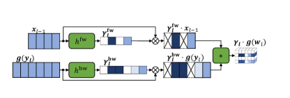
Figure 4. Meta attention of layer $l$ during on-device few-shot learning. Note that “Forward” part and “Backward” part are the same as Fig. 3, which are omitted for simplicity. Meta attention modules are not optimized during few-shot learning, thus are expressed as parameter-free functions $h^{\mathrm{fw}}$ and $h^{\mathrm{bw}}$. The input $\bm{x}_{l-1}$ stored during forward path is a sparse re-weighted tensor.

3.3.2. Exploiting Meta Attention for On-device Adaptation

We now explain how to apply the meta attention to save memory during on-device few-shot learning. Note that the parameters in the meta attention modules are fixed during few-shot learning. Assume that at step $k$, layer $l$ has a nonzero step size $\alpha_{l}^{k}$. In the forward pass, we only store a sparse tensor $\bm{\gamma}_{l}^{\mathrm{fw}}\cdot\bm{x}_{l-1}$, i.e., its channels are stored only if they correspond to nonzero entries in $\bm{\gamma}_{l}^{\mathrm{fw}}$. This reduces memory consumption as shown in Eq.(17) in Appendix A. Similarly, in the backward pass, we get a channel-wise sparse tensor $\bm{\gamma}_{l}^{\mathrm{bw}}\cdot\bm{g}(\bm{y}_{l})$. Since both sparse tensors are used to calculate the corresponding nonzero gradients in $\bm{g}(\bm{w}_{l})$, the computation cost is also reduced, see Eq.(18) in Appendix A. We plot the meta attention during on-device adaptation in Fig. 4.

3.4. Summary of p-Meta

Alg. 2 shows the overall process of p-Meta during meta-training. The final meta-trained weights $\bm{w}$ from Alg. 2 are assigned to $\bm{w}^{\mathrm{meta}}$, see Sec. 2. The meta-trained backbone model $F(\bm{w}^{\mathrm{meta}})$, the sparse inner step sizes $\bm{\alpha}$, and the meta attention modules will be then deployed on edge devices and used to conduct a memory-efficient few-shot learning.

3.5. Deployment Optimization

To further reduce the memory during few-shot learning, we propose gradient accumulation during backpropagation and replace batch normalization in the backbone with group normalization.

3.5.1. Gradient Accumulation

In standard few-shot learning, all the new samples (e.g., $25$ for $5$-way $5$-shot) are fed into the model as one batch. To reduce the peak memory due to large batch sizes, we conduct few-shot learning with gradient accumulation (GA).

GA is a technique that (i) breaks a large batch into smaller partial batches; (ii) sequentially forward/backward propagates each partial batches through the model; (iii) accumulates the loss gradients of each partial batch and get the final averaged gradients of the full batch. Note that GA does not increase computation, which is desired for low-resource platforms. We evaluate the impact of different sample batch sizes in GA in Appendix B.2.

3.5.2. Group Normalization

Mainstream backbones in meta learning typically adopt batch normalization layers. Batch normalization layers compute the statistical information in each batch, which is dependent on the sample batch size. When using GA with different sample batch sizes, the inaccurate batch statistics can degrade the training performance (see Appendix B.1). As a remedy, we use group normalization (Wu and He, 2018), which does not rely on batch statistics (i.e., independent of the sample batch size). We also apply meta attention on group normalization layers when updating their weights. The only difference w.r.t. conv and fc layers is that the stored input tensor (also the one used for the meta attention) is not $\bm{x}_{l-1}$, but its normalized version.

4. Evaluation

This section presents the evaluations of p-Meta on standard few-shot image classification and reinforcement learning benchmarks.

Table 2. Few-shot image classification results on 4Conv and ResNet12. All methods are meta-trained on MiniImageNet, and are few-shot learned on the reported datasets: MiniImageNet, TieredImageNet, and CUB (denoted by Mini, Tiered, and CUB in the table). The total computation (# GMACs) and the peak memory (MB) during few-shot learning are reported based on the theoretical analysis in Appendix A.

Benchmarks		5-way 1-shot					5-way 5-shot
		Mini	Tiered	CUB	Mini	Mini	Mini	Tiered	CUB	Mini	Mini
		Accuracy			GMAC	Memory	Accuracy			GMAC	Memory
4Conv	MAML (Finn et al., 2017)	46.2%	51.4%	39.7%	0.39	2.06	61.4%	66.5%	55.6%	1.96	2.06
	ANIL (Raghu et al., 2020)	46.4%	51.5%	39.2%	0.14	0.92	60.6%	64.5%	54.2%	0.72	0.92
	BOIL (Oh et al., 2021)	44.7%	51.3%	42.3%	0.39	2.05	60.5%	65.3%	58.3%	1.96	2.05
	MAML++ (Antoniou et al., 2019)	48.2%	53.2%	43.2%	0.39	2.06	63.7%	68.5%	59.1%	1.96	2.06
	p-Meta (3.2)	47.1%	52.3%	41.8%	0.16	1.00	62.9%	68.3%	59.3%	1.34	1.09
	p-Meta (3.2+3.3)	48.8%	53.9%	42.6%	0.15	0.99	65.0%	68.5%	60.2%	1.11	1.04
ResNet12	MAML (Finn et al., 2017)	51.7%	57.4%	41.3%	37.08	54.69	64.7%	69.6%	53.8%	185.42	54.69
	ANIL (Raghu et al., 2020)	50.3%	56.7%	40.6%	12.42	3.62	62.3%	68.7%	54.0%	62.08	3.62
	BOIL (Oh et al., 2021)	42.7%	47.7%	44.2%	37.08	54.69	53.6%	59.8%	53.7%	185.42	54.69
	MAML++ (Antoniou et al., 2019)	53.1%	58.6%	45.1%	37.08	54.69	68.6%	73.4%	63.9%	185.42	54.69
	p-Meta (3.2)	51.8%	58.3%	40.6%	25.84	17.66	68.8%	72.6%	65.9%	124.15	18.95
	p-Meta (3.2+3.3)	53.6%	59.4%	45.4%	24.02	16.01	69.7%	73.3%	66.6%	116.79	17.17

Table 3. Few-shot reinforcement learning results on 2D navigation and robot locomotion (larger return means better). A MLP with two hidden layers of size 100 is used as the policy model. The total computation (# GMACs) and the peak memory (MB) during few-shot learning are reported based on the theoretical analysis in Appendix A.

Benchmarks	20 Rollouts			20 Rollouts
	Half-Cheetah Velocity			2D Navigation
	Return	GMAC	Memory	Return	GMAC	Memory
MAML (Finn et al., 2017)	-82.2	0.15	0.24	-13.3	0.12	0.21
ANIL (Raghu et al., 2020)	-78.8	0.06	0.09	-13.8	0.04	0.08
BOIL (Oh et al., 2021)	-76.4	0.15	0.23	-12.4	0.12	0.21
MAML++ (Antoniou et al., 2019)	-69.6	0.15	0.24	-17.6	0.12	0.21
p-Meta (3.2)	-65.5	0.11	0.12	-11.2	0.09	0.09
p-Meta (3.2+3.3)	-64.0	0.11	0.11	-11.8	0.09	0.09

4.1. General Experimental Settings

Compared Methods. We test the meta learning algorithms below.

• MAML (Finn et al., 2017): the original model-agnostic meta learning.

• ANIL (Raghu et al., 2020): update the last layer only in few-shot learning.

• BOIL (Oh et al., 2021): update the body except the last layer.

• MAML++ (Antoniou et al., 2019): learn a per-step per-layer step sizes $\bm{\alpha}$.

• p-Meta (3.2): can be regarded as a sparse version of MAML++, since it learns a sparse $\bm{\alpha}$ with our methods in Sec. 3.2.

• p-Meta (3.2+3.3): the full version of our methods which include the meta attention modules in Sec. 3.3.

For fair comparison, all the algorithms are re-implemented with the deployment optimization in Sec. 3.5.

Implementation. The experiments are conducted with tools provided by TorchMeta (Deleu et al., 2019; Deleu, 2018). Particularly, the backbone is meta-trained with full sample batch size (e.g., 25 for 5-way 5-shot) on meta training dataset. After each meta training epoch, the model is tested (i.e., few-shot learned) on meta validation dataset. The model with the highest validation performance is used to report the final few-shot learning results on meta test dataset. We follow the same process as TorchMeta (Deleu et al., 2019; Deleu, 2018) to build the dataset. During few-shot learning, we adopt a sample batch size of 1 to verify the model performance under the most strict memory constraints.

In p-Meta, meta attention is applied to all conv, fc, and group normalization layers, except the last output layer, because (i) we find modifying the last layer’s gradients may decrease accuracy; (ii) the final output is often rather small in size, resulting in little memory saving even if imposing sparsity on the last layer. Without further notations, we set $\rho=0.3$ in forward attention, and $\rho=0$ in backward attention across all layers, as the sparsity of $\bm{\gamma}_{l}^{\mathrm{bw}}$ almost has no effect on the memory saving.

Metrics. We compare the peak memory and MACs of different algorithms. Note that the reported peak memory and MACs for p-Meta also include the consumption from meta attention, although they are rather small related to the backward propagation.

4.2. Performance on Image Classification

Settings. We test on standard few-shot image classification tasks (both in-domain and cross-domain). We adopt two common backbones, “4Conv” (Finn et al., 2017) which has 4 conv blocks with 32 channels in each block, and “ResNet12” (Oreshkin et al., 2018) which contains 4 residual blocks with $\{64,128,256,512\}$ channels in each block respectively. We replace the batch normalization layers with group normalization layers, as discussed in Sec. 3.5.2. We experiment in both 5-way 1-shot and 5-way 5-shot settings. We train the model on MiniImageNet (Vinyals et al., 2016) (both meta training and meta validation dataset) with 100 meta epochs. In each meta epoch, 1000 random tasks are drawn from the task distribution. The task batch size is set to 4 in general, except for ResNet12 under 5-way 5-shot settings where we use 2. The model is updated with 5 gradient steps (i.e., $K=5$) in both inner loop of meta-training and few-shot learning. We use Adam optimizer with cosine learning rate scheduling as (Antoniou et al., 2019) for all outer loop updating. The (initial) inner step size $\bm{\alpha}$ is set to 0.01. The meta-trained model is then tested on three datasets MiniImageNet (Vinyals et al., 2016), TieredImageNet (Ren et al., 2018), and CUB (Welinder et al., 2010) to verify both in-domain and cross-domain performance.

Results. Tab. 2 shows the accuracy averaged over $5000$ new unseen tasks randomly drawn from the meta test dataset. We also report the average number of GMACs and the average peak memory per task according to Appendix A. Clearly, p-Meta almost always yields the highest accuracy in all settings. Note that the comparison between “p-Meta (3.2)” and “MAML++” can be considered as the ablation studies on learning sparse layer-wise inner step sizes proposed in Sec. 3.2. Thanks to the imposed sparsity on $\bm{\alpha}$, “p-Meta (3.2)” significantly reduces the peak memory ($2.5\times$ saving on average and up to $3.1\times$) and the computation burden ($1.7\times$ saving on average and up to $2.4\times$) over “MAML++”. Note that the imposed sparsity also cause a moderate accuracy drop. However, with the meta attention, “p-Meta (3.2+3.3)” not only notably improves the accuracy but also further reduces the peak memory ($2.7\times$ saving on average and up to $3.4\times$) and computation ($1.9\times$ saving on average and up to $2.6\times$) over “MAML++”. “ANIL” only updates the last layer, and therefore consumes less memory but also yields a substantially lower accuracy.

4.3. Performance on Reinforcement Learning

Settings. To show the versatility of p-Meta, we experiment with two few-shot reinforcement learning problems: 2D navigation and Half-Cheetah robot locomotion simulated with MuJoCo library (Todorov et al., 2012). For all experiments, we mainly adopt the experimental setup in (Finn et al., 2017). We use a neural network policy with two hidden fc layers of size 100 and ReLU activation function. We adopt vanilla policy gradient (Williams, 1992) for the inner loop and trust-region policy optimization (Schulman et al., 2015) for the outer loop. During the inner loop as well as few-shot learning, the agents rollout 20 episodes with a horizon size of 200 and are updated for one gradient step. The policy model is trained for 500 meta epochs, and the model with the best average return during training is used for evaluation. The task batch size is set to 20 for 2D navigation, and 40 for robot locomotion. The (initial) inner step size $\bm{\alpha}$ is set to 0.1. Each episode is considered as a data sample, and thus the gradients are accumulated 20 times for a gradient step.

Results. Tab. 3 lists the average return averaged over 400 new unseen tasks randomly drawn from simulated environments. We also report the average number of GMACs and the average peak memory per task according to Appendix A. Note that the reported computation and peak memory do not include the estimations of the advantage (Duan et al., 2016), as they are relatively small and could be done during the rollout. p-Meta consumes a rather small amount of memory and computation, while often obtains the highest return in comparison to others. Therefore, p-Meta can fast adapt its policy to reach the new goal in the environment with less on-device resource demand.

4.4. Ablation Studies on Meta Attention

We study the effectiveness of our meta attention via the following two ablation studies. The experiments are conducted on “4Conv” in both 5-way 1-shot and 5-way 5-shot as Sec. 4.2.

Sparsity in Meta Attention. Tab. 4 shows the few-shot classification accuracy with different sparsity settings in the meta attention.

We first do not impose sparsity on $\bm{\gamma}_{l}^{\mathrm{fw}}$ and $\bm{\gamma}_{l}^{\mathrm{bw}}$ (i.e., set both $\rho$’s as 0), and adopt forward attention and backward attention separately. In comparison to no meta attention at all, enabling either forward or backward attention improves accuracy. With both attention enabled, the model achieves the best performance.

We then test the effects when imposing sparsity on $\bm{\gamma}_{l}^{\mathrm{fw}}$ or $\bm{\gamma}_{l}^{\mathrm{bw}}$ (i.e., set $\rho>0$). We use the same $\rho$ for all layers. We observe a sparse $\bm{\gamma}_{l}^{\mathrm{bw}}$ often cause a larger accuracy drop than a sparse $\bm{\gamma}_{l}^{\mathrm{fw}}$. Since a sparse $\bm{\gamma}_{l}^{\mathrm{bw}}$ does not bring substantial memory or computation saving (see Appendix A), we use $\rho=0$ for backward attention and $\rho=0.3$ for forward attention.

Attention scores $\bm{\gamma}_{l}$ introduce a dynamic channel-wise learning rate according to the new data samples. We further compare meta attention with a static channel-wise learning rate, where the channel-wise learning rate $\bm{\alpha}^{\mathrm{Ch}}$ is meta-trained as the layer-wise inner step sizes in Sec. 3.2 while without imposing sparsity. By comparing “$\bm{\alpha}^{\mathrm{Ch}}$” with “0, 0” in Tab. 4, we conclude that the dynamic channel-wise learning rate yields a significantly higher accuracy.

Table 4. Ablation results of meta attention on 4Conv.

$\rho$		5-way 1-shot			5-way 5-shot
fw	bw	Mini	Tiered	CUB	Mini	Tiered	CUB
x	x	47.1%	52.3%	41.8%	62.9%	68.3%	59.3%
0	x	48.1%	53.2%	41.7%	64.1%	68.4%	59.0%
x	0	47.8%	53.1%	40.9%	63.9%	68.5%	60.0%
0	0	49.0%	54.2%	43.1%	64.5%	69.2%	60.2%
0	0.3	48.5%	53.4%	42.2%	64.7%	68.2%	59.3%
0.3	0	48.8%	53.9%	42.6%	65.0%	68.5%	60.2%
0.3	0.3	48.7%	53.7%	42.3%	64.5%	68.3%	59.5%
0.5	0.5	48.2%	53.4%	42.7%	64.8%	68.1%	59.1%
$\bm{\alpha}^{\mathrm{Ch}}$		47.8%	52.8%	41.0%	63.6%	68.1%	58.1%

• x: no forward/backward meta attention, i.e., $\bm{\gamma}_{l}^{\mathrm{fw}}=1$ or $\bm{\gamma}_{l}^{\mathrm{bw}}=1$.

• $\bm{\alpha}^{\mathrm{Ch}}$: introducing an input- and output-channel-wise inner step sizes $\bm{\alpha}^{\mathrm{Ch}}$ per layer. We use $\bm{\alpha}\cdot\bm{\alpha}^{\mathrm{Ch}}$ as the overall inner step sizes. $\bm{\alpha}^{\mathrm{Ch}}$ is meta-trained as $\bm{\alpha}$ without imposing sparsity.

Layer-wise Updating Ratios. To study the resulted updating ratios across layers, i.e., the layer-wise sparsity of weight gradients, we randomly select 100 new tasks and plot the layer-wise updating ratios, see Fig. 5 Left (1:5). The “4Conv” backbone has 9 layers ($L=9$), i.e., 8 alternates of conv and group normalization layers, and an fc output layer. As mentioned in Sec. 4.1, we do not apply meta attention to the output layer, i.e., $\bm{\gamma}_{9}=1$. The used backbone is updated with 5 gradient steps ($K=5$). We use $\rho=0.3$ for forward attention, and $\rho=0$ for backward. Note that Alg. 1 adaptively determines the sparsity of $\bm{\gamma}_{l}$, which also means different samples may result in different updating ratios even with the same $\rho$ (see Fig. 5). The size of $\bm{x}_{l-1}$ often decreases along the layers in current DNNs. As expected, the latter layers are preferred to be updated more, since they need a smaller amount of memory for updating. Interestingly, even if with a small $\rho$($=0.3$), the ratio of updated weights is rather small, e.g., smaller than $0.2$ in step 3 of 5-way 5-shot. It implies that the outputs of softmax have a large discrepancy, i.e., only a few channels are adaptation-critical for each sample, which in turn verifies the effectiveness of our meta attention mechanism.

We also randomly pair data samples and compute the cosine similarity between their attention scores $\bm{\gamma}_{l}$. We plot the cosine similarity of step 1 in Fig. 5 Right. The results show that there may exist a considerable variation on the adaptation-critical weights selected by different samples, which is consistent with our observation in Tab. 4, i.e., dynamic learning rate outperforms the static one.

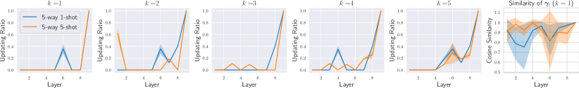
Figure 5. Left (1:5): Layer-wise updating ratios (mean $\pm$ standard deviation) in each updating step. Note that the ratio of updated weights is determined by both static layer-wise inner step sizes $\alpha_{1:L}^{1:K}$ and the dynamic meta attention scores $\bm{\gamma}_{1:L}$. The layer with an updating ratio of 0 means its $\alpha=0$. Right: Cosine similarity (mean $\pm$ standard deviation) of $\bm{\gamma}_{1:L}$ between random pair of data samples. The results are reported in step 1, because all samples are fed into the same initial model in step 1.

5. Related Work

Meta Learning for Few-Shot Learning. Meta learning is a prevailing solution to few-shot learning (Hospedales et al., 2020), where the meta-trained model can learn an unseen task from a few training samples, i.e., data-efficient adaptation. The majority of meta learning methods can be divided into two categories, (i) metric-based methods (Vinyals et al., 2016; Snell et al., 2017; Sung et al., 2018) that learn an embedded metric for classification tasks to map the query samples onto the classes of labeled support samples, (ii) gradient-based methods (Antoniou et al., 2019; Finn et al., 2017; Raghu et al., 2020; Triantafillou et al., 2020; Oh et al., 2021; Von Oswald et al., 2021) that learn an initial model (and/or optimizer parameters) such that it can be adapted with gradient information calculated on the new few samples. In comparison to metric-based methods, we focus on gradient-based meta learning methods for their wide applicability in various learning tasks (e.g., regression, classification, reinforcement learning) and the availability of gradient-based training frameworks for low-resource devices (TensorFlow, [n.d.]).

Particularly, we aim at meta training a DNN that allows effective adaptation on memory-constrained devices. Most meta learning algorithms (Antoniou et al., 2019; Finn et al., 2017; Von Oswald et al., 2021) optimize the backbone network for better generalization yet ignore the workload if the meta-trained backbone is deployed to low-resource platforms for model adaptation. Manually fixing certain layers during on-device few-shot learning (Raghu et al., 2020; Oh et al., 2021; Shen et al., 2021) may also reduce memory and computation, but to a much lesser extent as shown in our evaluations.

Efficient DNN Training. Existing efficient training schemes are mainly designed for high-throughput GPU training on large-scale datasets. A general strategy is to trade memory with computation (Chen et al., 2016; Gruslys et al., 2016), which is unfit for IoT device with a limited computation capability. An alternative is to sparsify the computational graphs in backpropagation (Raihan and Aamodt, 2020). Yet it relies on massive training iterations on large-scale datasets. Other techniques include layer-wise local training (Greff et al., 2017) and reversible residual module (Gomez et al., 2017), but they often incur notable accuracy drops.

There are a few studies on DNN training on low-resource platforms, such as updating the last several layers only (Mathur et al., 2021), reducing batch sizes (Lee and Nirjon, 2019), and gradient approximation (Gooneratne et al., 2020). However, they are designed for vanilla supervised training, i.e., train and test on the same task. One recent study proposes to update the bias parameters only for memory-efficient transfer learning (Cai et al., 2020), yet transfer learning is prone to overfitting when trained with limited data (Finn et al., 2017).

6. Conclusion

In this paper, we present p-Meta, a new meta learning scheme for data- and memory-efficient on-device DNN adaptation. It enables structured partial parameter updates for memory-efficient few-shot learning by automatically identifying adaptation-critical weights both layer-wise and channel-wise. Evaluations show a reduction in peak dynamic memory by 2.5$\times$ on average over the state-of-the-art few-shot adaptation methods. We envision p-Meta as an early step towards adaptive and autonomous edge intelligence applications.

Appendix A Memory and Computation

In the following, we derive the memory requirement and computation workload for inference and adaptation. We restrict ourselves to a feed-forward network of fully-connected (fc) or convolutional (conv) layers. Note that our analysis focuses on 2D conv layers but can apply to other conv layer types as well. We assume the rectified linear activation function (ReLU) for all layers, denoted as $\sigma$. For simplicity, we omit the bias, normalization layers, pooling or strides. We use the notation $m(\bm{x})$ to denote the memory demand in words to store tensor $\bm{x}$. The wordlength is denoted as $\mathit{T}$.

For representing indexed summations we use the Einstein notation. If index variables appear in a term on the right hand side of an equation and are not otherwise defined (free indices), it implies summation of that term over the range of the free indices. If indices of involved tensor elements are out of range, the values of these elements are assumed to be 0.

A.1. Single Layer

We start with a single layer and accumulate the memory and computation for networks with several layers afterwards. Assume the input tensor of a layer is $\bm{x}$, the weight tensor is $\bm{w}$, the result after the linear transformation is $\bm{y}$, and the layer output after the non-linear operator is $\bm{z}$ which is also the input to the next layer.

For convolutional layers, we have $\bm{x}\in\mathbb{R}^{C_{I}\times H_{I}\times W_{I}}$ and elements $x_{cij}$, where $C_{I}$, $H_{I}$, and $W_{I}$ denote the number of input channels, height and width, respectively. In a similar way, we have $\bm{z}\in\mathbb{R}^{C_{O}\times H_{O}\times W_{O}}$ with elements $x_{fij}$ where $C_{O}$, $H_{O}$, and $W_{O}$ denote the number of output channels, height and width, respectively. Moreover, $\bm{w}\in\mathbb{R}^{C_{O}\times C_{I}\times S\times S}$ with elements $w_{fcmn}$. Therefore,

$$\medop{m(\bm{x})=C_{I}H_{I}W_{I}\;,\;\;m(\bm{y})=m(\bm{z})=C_{O}H_{O}W_{O}\;,\;\;m(\bm{w})=C_{O}C_{I}S^{2}}$$

For fully connected layers we have $\bm{x}\in\mathbb{R}^{C_{I}}$, $\bm{y},\bm{z}\in\mathbb{R}^{C_{O}}$, and $\bm{w}\in\mathbb{R}^{C_{O}\times C_{I}}$ with memory demand

$$\medop{m(\bm{x})=C_{I}\;,\;\;m(\bm{y})=m(\bm{z})=C_{O}\;,\;\;m(\bm{w})=C_{O}C_{I}}$$

A.1.1. Fully Connected Layer

For inference we derive the relations $y_{f}=w_{fc}x_{c}$ and $z_{f}=\sigma(y_{f})$ for all admissible indices $f\in[1,C_{O}]$. The necessary dynamic memory has a size of about $m(\bm{x})+m(\bm{y})$ words and we need about $m(\bm{w})$ MAC operations.

For adaptation, we suppose that $\frac{\partial\ell}{\partial z_{i}}$ is already provided from the next layer. We find $\frac{\partial\ell}{\partial y_{i}}=\sigma^{\prime}(y_{i})\cdot\frac{\partial\ell}{\partial z_{i}}$ with $\sigma^{\prime}(y_{i})=\begin{cases}1&\mbox{if }y_{i}>0\\ 0&\mbox{if }y_{i}<0\end{cases}$ which leads to $\frac{\partial\ell}{\partial x_{i}}=w_{ji}\cdot\frac{\partial\ell}{\partial y_{j}}$. The necessary dynamic memory is about $m(\bm{x})+m(\bm{y})\cdot(1+\frac{1}{\mathit{T}})$ words, where the last term comes from storing $\sigma^{\prime}(y_{i})$ single bits from the forward path. We need about $m(\bm{w})$ MAC operations.

According to the approach described in the paper we are only interested in the partial derivatives $\frac{\partial\ell}{\partial w_{fc}}$ if $\alpha>0$ for this layer, and if scales $\gamma^{\mathrm{bw}}_{f}>0$ and $\gamma^{\mathrm{fw}}_{c}>0$ for indices $f$, $c$. To simplify the notation, let us define the critical ratios

$$\medop{\mu^{\mathrm{fw}}=\frac{\text{number of nonzero elements of }\gamma^{\mathrm{fw}}_{c}}{C_{I}}}$$

$$\medop{\mu^{\mathrm{bw}}=\frac{\text{number of nonzero elements of }\gamma^{\mathrm{bw}}_{f}}{C_{O}}}$$

which are 1 if all channels are determined to be critical for weight adaptation, and 0 if none of them.

We find $\gamma^{\mathrm{bw}}_{f}\frac{\partial\ell}{\partial w_{fc}}\gamma^{\mathrm{fw}}_{c}=(\gamma^{\mathrm{bw}}_{f}\frac{\partial\ell}{\partial y_{f}})\cdot(\gamma^{\mathrm{fw}}_{c}x_{c})$. Therefore, we need $\mu^{\mathrm{fw}}\mu^{\mathrm{bw}}m(\bm{w})+\mu^{\mathrm{fw}}m(\bm{x})$ words dynamic memory if $\alpha>0$ where the latter term considers the information needed from the forward path. We require about $\mu^{\mathrm{fw}}\mu^{\mathrm{bw}}m(\bm{w})$ MAC operations if $\alpha>0$.

A.1.2. Convolutional Layer

The memory analysis for a convolutional layer is very similar, just replacing matrix multiplication by convolution. For inference we find $y_{fij}=w_{fcmn}x_{c,i+m-1,j+n-1}$ and $z_{fij}=\sigma(y_{fij})$ for all admissible indices $f$, $i$, $j$. The necessary dynamic memory has a size of about $\max\{m(\bm{x}),m(\bm{y})\}$ words when using memory sharing between input and output tensors. We need about $H_{O}W_{O}\cdot m(\bm{w})$ MAC operations.

For adaptation, we again suppose that $\frac{\partial\ell}{\partial z_{fij}}$ is provided from the next layer. We find $\frac{\partial\ell}{\partial y_{fij}}=\sigma^{\prime}(y_{fij})\cdot\frac{\partial\ell}{\partial z_{fij}}$ and get $\frac{\partial\ell}{\partial x_{cij}}=w_{fcmn}\cdot\frac{\partial\ell}{\partial y_{f,i+m-1,j+n-1}}$. The necessary memory is about $\max\{m(\bm{x}),m(\bm{y})\}+\frac{m(\bm{y})}{\mathit{T}}$ words, where the last term comes from storing $\sigma^{\prime}(y_{fij})$ single bits from the forward path. We need about $H_{I}W_{I}\cdot m(\bm{w})$ multiply and accumulate operations.

For determining the weight gradients we find $\frac{\partial\ell}{\partial w_{fcmn}}=\frac{\partial\ell}{\partial y_{fij}}\cdot x_{c,i+m-1,j+n-1}$. When considering the scales for filtering, we yield $\gamma^{\mathrm{bw}}_{f}\frac{\partial\ell}{\partial w_{fcmn}}\gamma^{\mathrm{fw}}_{c}=(\gamma^{\mathrm{bw}}_{f}\frac{\partial\ell}{\partial y_{fij}})\cdot(\gamma^{\mathrm{fw}}_{c}x_{c,i+m-1,j+n-1})$. As a result, we need $\mu^{\mathrm{fw}}\mu^{\mathrm{bw}}m(\bm{w})+\mu^{\mathrm{fw}}m(\bm{x})$ words of dynamic memory if $\alpha>0$ where the latter term considers the information needed from the forward path. We require about $\mu^{\mathrm{fw}}\mu^{\mathrm{bw}}H_{O}W_{O}m(\bm{w})$ MAC operations if $\alpha>0$.

Finally, let us determine the required memory and computation to determine the scales $\gamma^{\mathrm{fw}}_{c}$ and $\gamma^{\mathrm{bw}}_{f}$. According to Fig. 3, we find as an upper bound for the memory $B\cdot(C_{I}+C_{O})$ and $(C_{I}H_{I}W_{I}+2C_{I}^{2}+C_{O}H_{O}W_{O}+2C_{O}^{2})$ MAC operations.

A.2. All Layers

The above relations are valid for a single layer. The following relations hold for the overall network. In order to simplify the notation, we consider a network that consists of convolution layers only. Extensions to mixed layers can simply be done.

We suppose $L$ layers with sizes $C_{l}$, $H_{l}$, $W_{l}$ and $S_{l}$ for the number of output channels, output width, output height and kernel size, respectively. We assume that the step-sizes $\alpha_{l}$ for some iteration of the adaption are given. The memory requirement in words is

$$\medop{m(\bm{x}_{l})=C_{l}H_{l}W_{l}\;,\;\;m(\bm{w}_{l})=C_{l}C_{l-1}S_{l}^{2}}$$

and the word-length is again denoted as $\mathit{T}$. We define as $\hat{\alpha}_{l}=\begin{cases}1&\mbox{if }\alpha_{l}>0\\ 0&\mbox{if }\alpha_{l}=0\end{cases}$ the mask that determines whether the weight adaptation for this layer is necessary or not.

Let us first look at the forward path. The necessary dynamic memory is about $\max_{0\leq l\leq L}\{m(\bm{x}_{l})\}$ words. The amount of MAC operations is $\sum_{1\leq l\leq L}H_{l}W_{l}m(\bm{w}_{l})$.

The backward path needs only to be evaluated until we reach the first layer where we require the computation of the gradients. We define $l_{\mathit{min}}=\min\{l\,|\,\hat{\alpha}_{l}=1\}$. For the calculation of the partial derivatives of the activations we need dynamic memory of $\max_{l_{\mathit{min}}\leq l\leq L}\{m(\bm{x}_{l})\}+\frac{1}{\mathit{T}}\sum_{l_{\mathit{min}}\leq l\leq L}m(\bm{x}_{l})$ words where the last term is due to storing the derivatives of the ReLU operations. We need about $\sum_{l_{\mathit{min}}+1\leq l\leq L}H_{l-1}W_{l-1}m(\bm{w}_{l})$ MAC operations.

The second contribution of the backward path is for computing the weight gradients. The memory and computation demand of the scales will be neglected as they are much smaller than other contributions. We can determine the necessary dynamic memory as $\max_{1\leq l\leq L}\{\hat{\alpha}_{l}\mu^{\mathrm{fw}}_{l}\mu^{\mathrm{bw}}_{l}m(\bm{w}_{l})\}+\sum_{1\leq l\leq L}\hat{\alpha}_{l}\mu^{\mathrm{fw}}_{l}m(\bm{x}_{l-1})$, and we need $\sum_{1\leq l\leq L}\hat{\alpha}_{l}\mu^{\mathrm{fw}}_{l}\mu^{\mathrm{bw}}_{l}H_{l}W_{l}m(\bm{w}_{l})$ MAC operations.

Considering all necessary dynamic memory with memory reuse for an adaptation step, we get an estimation of memory in words

(16) $$\medop{\max_{0\leq l\leq L}\{m(\bm{x}_{l})\}+\sum_{1\leq l\leq L}\hat{\alpha}_{l}m(\bm{w}_{l})+}\\ \medop{+\sum_{1\leq l\leq L}\hat{\alpha}_{l}\mu^{\mathrm{fw}}_{l}m(\bm{x}_{l-1})+\frac{1}{\mathit{T}}\sum_{l_{\mathit{min}}\leq l\leq L}m(\bm{x}_{l})}$$

if we accumulate the weight gradients before doing an SGD step and re-use some memory during back-propagation. More elaborate memory re-use can be used to slightly sharpen the bounds without a major improvement. For conventional training, each parameter is in 32-bit floating point format, i.e., one word corresponds to 32-bit. As discussed in Sec. 2, we only consider max-pooling and ReLU-styled activation as the $\sigma$ function. The wordlength $T$ in Eq.(16) is set as 16 for max-pooling , and 32 for ReLU-styled activation. One can see that under the typical assumptions for network parameters, the above memory requirement in words is dominated by

(17) $$\medop{\sum_{1\leq l\leq L}\hat{\alpha}_{l}\mu^{\mathrm{fw}}_{l}m(\bm{x}_{l-1})}$$

The necessary storage between the forward and backward path is reduced proportionally to $\mu^{\mathrm{fw}}_{l}$ with factor $m(\bm{x}_{l-1})$.

Finally, the amount of MAC computations can be estimated as

(18) $$\medop{\sum_{1\leq l\leq L}H_{l}W_{l}m(\bm{w}_{l})(1+\hat{\alpha}_{l}\mu^{\mathrm{fw}}_{l}\mu^{\mathrm{bw}}_{l})+\sum_{l_{\mathit{min}}\leq l\leq L}H_{l-1}W_{l-1}m(\bm{w}_{l})}$$

while neglecting lower order terms. Here it is important to note that all terms are of similar order. The approach used in the paper does not determine a trade-off between computation and memory, but reduces the amount of MAC operations. This reduction is less than the reduction in required dynamic memory.

Appendix B Other Experiments

B.1. Pooling & Normalization

In this section, we test the backbone network with different types of pooling and normalization. Without further notations in the following experiments, we meta-train our “4Conv” backbone on MiniImageNet with full batch sizes, and conduct few-shot learning with gradient accumulation with a batch size of 1, as in Sec. 4. Here, we report the results with the original “MAML” method (Finn et al., 2017) in Tab. 5. Clearly, the discrepancy of batch statistics between meta-training phase and few-shot learning phase causes a large accuracy loss in batch normalization layers. Batch normalization works only if few-shot learning uses full batch sizes, i.e., without gradient accumulation, which however does not fit in our memory-constrained scenarios (see Sec. 3.5.1). In addition, max-pooling performs better than average-pooling. We thus use group normalization and max-pooling in our backbone model, see Sec. 4.

Table 5. Comparison between different pooling and normalization layers.

4Conv		5-way 1-shot
Pooling	Norm.	Mini	Tiered	CUB
Average	Batch	25.3%	27.2%	26.1%
Average	Group	45.8%	50.3%	40.2%
Max	Batch	27.6%	28.9%	26.5%
Max	Group	46.2%	51.4%	39.9%

B.2. Sample Batch Size

In this section, we show the effects brought from different sample batch sizes. During few-shot learning phase, gradient accumulation is applied to fit in different on-device memory constraints. We report the accuracy when adopting different sample batch sizes in gradient accumulation. Although group normalization eliminates the variance of batch statistics, adopting different batch sizes may still result in diverse performance due to the batch-averaged scores in meta attention. The results in Tab. 6 show that different batch sizes yield a similar accuracy level, which indicates that our meta attention module is relatively robust to batch sizes.

Table 6. Ablation results of sample batch sizes.

	5-way 1-shot			5-way 5-shot
Batch Size	1	2	5	1	5	25
Mini	48.8%	48.7%	48.3%	65.0%	65.1%	64.7%
Tiered	53.9%	53.6%	54.3%	68.5%	68.9%	68.1%
CUB	42.6%	42.1%	42.4%	60.2%	59.5%	60.6%

B.3. Sparse x and Sparse g(y)

Our meta attention modules take $\bm{x}_{l-1}$ and $\bm{g}(\bm{y}_{l})$ as inputs, and output attention scores which are used to create sparse $\bm{g}(\bm{w}_{l})$. However, applying the resulted sparse attention scores on $\bm{x}_{l-1}$ and $\bm{g}(\bm{y}_{l})$ can also bring memory and computation benefits, as discussed in Sec. 3.1. We conduct the ablations when multiplying attention scores $\bm{\gamma}_{l}^{\mathrm{fw}}$ and $\bm{\gamma}_{l}^{\mathrm{bw}}$ on $\bm{g}(\bm{w}_{l})$ (also the one used in the main text), or on $\bm{x}_{l-1}$ and $\bm{g}(\bm{y}_{l})$ respectively. The results in Tab. 7 show that a channel-wise sparse $\bm{x}_{l-1}$ hugely degrades the performance, in comparison to only imposing sparsity on $\bm{g}(\bm{w}_{l})$ while using a dense $\bm{x}_{l-1}$ in the forward pass. In addition, directly adopting a sparse $\bm{g}(\bm{y}_{l})$ in backpropagation may even cause non-convergence in few-shot learning. We think this is due to the fact that the error accumulates along the propagation when imposing sparsity on $\bm{x}_{l-1}$ or $\bm{g}(\bm{y}_{l})$.

Table 7. Ablation results of sparse $\bm{x}_{l-1}$ and sparse $\bm{g}(\bm{y}_{l})$.

$\rho=0.3$		5-way 1-shot			5-way 5-shot
fw	bw	Mini	Tiered	CUB	Mini	Tiered	CUB
x	x	47.1%	52.3%	41.8%	62.9%	68.3%	59.3%
$\bm{g}(\bm{w}_{l})$	x	48.2%	53.6%	41.2%	63.6%	69.0%	59.0%
$\bm{x}_{l-1}$	x	37.4%	37.9%	35.4%	47.9%	49.3%	42.5%
x	$\bm{g}(\bm{w}_{l})$	48.0%	53.0%	42.6%	64.0%	67.8%	59.9%
x	$\bm{g}(\bm{y}_{l})$	22.8%	21.1%	20.6%	20.7%	21.0%	20.4%

• x: no forward/backward (sparse) meta attention, i.e., $\bm{\gamma}_{l}^{\mathrm{fw}}=1$ or $\bm{\gamma}_{l}^{\mathrm{bw}}=1$.

References

- (1)
- Antoniou et al. (2019) Antreas Antoniou, Harrison Edwards, and Amos Storkey. 2019. How to train your MAML. In ICLR.
- Cai et al. (2020) Han Cai, Chuang Gan, Ligeng Zhu, and Song Han. 2020. TinyTL: Reduce Memory, Not Parameters for Efficient On-Device Learning. In NeurIPS.
- Chen et al. (2021) Beidi Chen, Zichang Liu, Binghui Peng, Zhaozhuo Xu, Jonathan Lingjie Li, Tri Dao, Zhao Song, Anshumali Shrivastava, and Christopher Re. 2021. MONGOOSE: A Learnable LSH Framework for Efficient Neural Network Training. In ICLR.
- Chen et al. (2016) Tianqi Chen, Bing Xu, Chiyuan Zhang, and Carlos Guestrin. 2016. Training deep nets with sublinear memory cost. arXiv:1604.06174
- Chen et al. (2020) Yinpeng Chen, Xiyang Dai, Mengchen Liu, Dongdong Chen, Lu Yuan, and Zicheng Liu. 2020. Dynamic Convolution: Attention Over Convolution Kernels. In CVPR.
- Deleu (2018) Tristan Deleu. 2018. Model-Agnostic Meta-Learning for Reinforcement Learning in PyTorch. Available at: https://github.com/tristandeleu/pytorch-maml-rl.
- Deleu et al. (2019) Tristan Deleu, Tobias Würfl, Mandana Samiei, Joseph Paul Cohen, and Yoshua Bengio. 2019. Torchmeta: A Meta-Learning library for PyTorch. https://arxiv.org/abs/1909.06576 Available at: https://github.com/tristandeleu/pytorch-meta.
- Deng et al. (2020) Lei Deng, Guoqi Li, Song Han, Luping Shi, and Yuan Xie. 2020. Model compression and hardware acceleration for neural networks: a comprehensive survey. Proc. IEEE 108, 4 (2020), 485–532.
- Duan et al. (2016) Yan Duan, Xi Chen, Rein Houthooft, John Schulman, and Pieter Abbeel. 2016. Benchmarking Deep Reinforcement Learning for Continuous Control. In ICML.
- Finn et al. (2017) Chelsea Finn, Pieter Abbeel, and Sergey Levine. 2017. Model-agnostic meta-learning for fast adaptation of deep networks. In ICML.
- Gao et al. (2021) Dawei Gao, Xiaoxi He, Zimu Zhou, Yongxin Tong, and Lothar Thiele. 2021. Pruning meta-trained networks for on-device adaptation. In CIKM.
- Gomez et al. (2017) Aidan N Gomez, Mengye Ren, Raquel Urtasun, and Roger B Grosse. 2017. The Reversible Residual Network: Backpropagation Without Storing Activations. In NeurIPS.
- Gong et al. (2019) Taesik Gong, Yeonsu Kim, Jinwoo Shin, and Sung-Ju Lee. 2019. Metasense: few-shot adaptation to untrained conditions in deep mobile sensing. In SenSys.
- Goodfellow et al. (2016) Ian Goodfellow, Yoshua Bengio, Aaron Courville, and Yoshua Bengio. 2016. Deep learning. Vol. 1. MIT press Cambridge.
- Gooneratne et al. (2020) Mary Gooneratne, Khe Chai Sim, Petr Zadrazil, Andreas Kabel, Françoise Beaufays, and Giovanni Motta. 2020. Low-rank Gradient Approximation For Memory-Efficient On-device Training of Deep Neural Network. In ICASSP.
- Goyal et al. (2017) Priya Goyal, Piotr Dollár, Ross Girshick, Pieter Noordhuis, Lukasz Wesolowski, Aapo Kyrola, Andrew Tulloch, Yangqing Jia, and Kaiming He. 2017. Accurate, large minibatch sgd: Training imagenet in 1 hour. arXiv:1706.02677
- Greff et al. (2017) Klaus Greff, Rupesh K. Srivastava, and Jürgen Schmidhuber. 2017. Highway and Residual Networks learn Unrolled Iterative Estimation. In NeurIPS.
- Gruslys et al. (2016) Audrūnas Gruslys, Remi Munos, Ivo Danihelka, Marc Lanctot, and Alex Graves. 2016. Memory-Efficient Backpropagation Through Time. In NeurIPS.
- Gui et al. (2018) Liang-Yan Gui, Yu-Xiong Wang, Deva Ramanan, and José MF Moura. 2018. Few-shot human motion prediction via meta-learning. In ECCV.
- Han et al. (2016) Song Han, Huizi Mao, and William J Dally. 2016. Deep compression: Compressing deep neural networks with pruning, trained quantization and huffman coding. In ICLR.
- He et al. (2016) Kaiming He, Xiangyu Zhang, Shaoqing Ren, and Jian Sun. 2016. Deep Residual Learning for Image Recognition. In CVPR.
- Hospedales et al. (2020) Timothy Hospedales, Antreas Antoniou, Paul Micaelli, and Amos Storkey. 2020. Meta-learning in neural networks: a survey. arXiv:2004.05439
- Hu et al. (2018) Jie Hu, Li Shen, and Gang Sun. 2018. Squeeze-and-Excitation Networks. In CVPR.
- Lee and Nirjon (2019) Seulki Lee and Shahriar Nirjon. 2019. Neuro.ZERO: a zero-energy neural network accelerator for embedded sensing and inference systems. In SenSys.
- Mathur et al. (2021) Akhil Mathur, Daniel J. Beutel, Pedro Porto Buarque de Gusmão, Javier Fernandez-Marques, Taner Topal, Xinchi Qiu, Titouan Parcollet, Yan Gao, and Nicholas D. Lane. 2021. On-device Federated Learning with Flower. In MLSys.
- Oh et al. (2021) Jaehoon Oh, Hyungjun Yoo, ChangHwan Kim, and Se-Young Yun. 2021. BOIL: Towards Representation Change for Few-shot Learning. In ICLR.
- Oreshkin et al. (2018) Boris N. Oreshkin, Pau Rodriguez, and Alexandre Lacoste. 2018. TADAM: Task dependent adaptive metric for improved few-shot learning. In NeurIPS.
- Raghu et al. (2020) Aniruddh Raghu, Maithra Raghu, Samy Bengio, and Oriol Vinyals. 2020. Rapid learning or feature reuse? Towards understanding the effectiveness of MAML. In ICLR.
- Raihan and Aamodt (2020) Md Aamir Raihan and Tor M. Aamodt. 2020. Sparse Weight Activation Training. In NeurIPS.
- Ren et al. (2018) Mengye Ren, Eleni Triantafillou, Sachin Ravi, Jake Snell, Kevin Swersky, Joshua B. Tenenbaum, Hugo Larochelle, and Richard S. Zemel. 2018. Meta-Learning for Semi-Supervised Few-Shot Classification. In ICLR.
- Russakovsky et al. (2015) Olga Russakovsky, Jia Deng, Hao Su, Jonathan Krause, Sanjeev Satheesh, Sean Ma, Zhiheng Huang, Andrej Karpathy, Aditya Khosla, Michael Bernstein, Alexander C. Berg, and Li Fei-Fei. 2015. ImageNet large scale visual recognition challenge. International Journal of Computer Vision 115, 3 (2015), 211–252.
- Schulman et al. (2015) John Schulman, Sergey Levine, Philipp Moritz, Michael I. Jordan, and Pieter Abbeel. 2015. Trust Region Policy Optimization. In ICML.
- Shen et al. (2021) Zhiqiang Shen, Zechun Liu, Jie Qin, Marios Savvides, and Kwang-Ting Cheng. 2021. Partial Is Better Than All: Revisiting Fine-tuning Strategy for Few-shot Learning. In AAAI.
- Snell et al. (2017) Jake Snell, Kevin Swersky, and Richard S. Zemel. 2017. Prototypical Networks for Few-shot Learning. In NeurIPS.
- Sung et al. (2018) Flood Sung, Yongxin Yang, Li Zhang, Tao Xiang, Philip H. S. Torr, and Timothy M. Hospedales. 2018. Learning to Compare: Relation Network for Few-Shot Learning. In CVPR.
- TensorFlow ([n.d.]) TensorFlow. [n.d.]. On-Device Training with TensorFlow Lite. https://www.tensorflow.org/lite/examples/on_device_training/overview. Accessed: 2022-01-15.
- Todorov et al. (2012) Emanuel Todorov, Tom Erez, and Yuval Tassa. 2012. Mujoco: A physics engine for model-based control. In IROS.
- Triantafillou et al. (2020) Eleni Triantafillou, Tyler Zhu, Vincent Dumoulin, Pascal Lamblin, Utku Evci, Kelvin Xu, Ross Goroshin, Carles Gelada, Kevin Swersky, Pierre-Antoine Manzagol, and Hugo Larochelle. 2020. Meta-Dataset: A Dataset of Datasets for Learning to Learn from Few Examples. In ICLR.
- Vinyals et al. (2016) Oriol Vinyals, Charles Blundell, Timothy Lillicrap, Koray Kavukcuoglu, and Daan Wierstra. 2016. Matching Networks for One Shot Learning. In NeurIPS.
- Von Oswald et al. (2021) Johannes Von Oswald, Dominic Zhao, Seijin Kobayashi, Simon Schug, Massimo Caccia, Nicolas Zucchet, and João Sacramento. 2021. Learning where to learn: Gradient sparsity in meta and continual learning. In NeurIPS.
- Welinder et al. (2010) P. Welinder, S. Branson, T. Mita, C. Wah, F. Schroff, S. Belongie, and P. Perona. 2010. Caltech-UCSD Birds 200. Technical Report CNS-TR-2010-001. California Institute of Technology.
- Williams (1992) Ronald J. Williams. 1992. Simple Statistical Gradient-Following Algorithms for Connectionist Reinforcement Learning. Mach. Learn. 8, 3–4 (may 1992). https://doi.org/10.1007/BF00992696
- Wu and He (2018) Yuxin Wu and Kaiming He. 2018. Group Normalization. In ECCV.