Towards Modern Card Games with Large-Scale Action Spaces Through Action Representation

Abstract

Axie infinity is a complicated card game with a huge-scale action space. This makes it difficult to solve this challenge using generic Reinforcement Learning (RL) algorithms. We propose a hybrid RL framework to learn action representations and game strategies. To avoid evaluating every action in the large feasible action set, our method evaluates actions in a fixed-size set which is determined using action representations. We compare the performance of our method with the other two baseline methods in terms of their sample efficiency and the winning rates of the trained models. We empirically show that our method achieves an overall best winning rate and the best sample efficiency among the three methods.

I Introduction

Games have facilitated the rapid development of RL algorithms in recent years. Card games, as a classical type of games, also pose many challenges to RL algorithms. The direct applications of generic algorithms [1, 2, 3, 4] in card games are problematic in many aspects because of the large-scale discrete action space [5]. Prior works have proposed RL methods to approach a number of traditional card games, like Texas Hold’em [6, 7, 8], Mahjong [9], DouDizhu [5, 10], etc. However, the issues brought by the large action space still remain, especially for modern card games such as Axie Infinity which has a huge discrete action space.

Axie Infinity is an one-versus-one online card game which has millions of players globally. Axies are virtual pets that have different attributes such as species, health, speed, etc. Each axie has its own card deck consisting of 2 copies of 4 cards. The player needs to form a team of 3 axies at the beginning and play their cards (24 cards in total) to beat the opponent player’s team.

This game is different from the traditional card game in the following aspects:

1. For a fixed team, the player needs to choose one sequence of cards from 23 million different card sequences.

2. The effect of a card is usually influenced by the its position in the card sequence and the status of the axies such as the health and the shield.

3. There are thousands of teams for players to choose. The optimal strategies for different teams are various.

These difficulties are all connected to the large-scale action space, and they are shared by a lot of other modern card games such as Hearthstone.

Some existing works have investigated the large action space issue in card games. Zha et al. [5] propose an action encoding scheme for DouDizhu. However, this encoding scheme cannot properly encode the action in our problem as the complexity of the action space in our problem is much higher than that in DouDizhu (27472 possible moves). Dulac-Arnold et al. [11] propose to choose actions in a small subset of the action space to speed up the action search process. This set is chosen based on a proper action encoding method which usually relies on prior knowledge. However, the prior human knowledge for our problem is hard to obtain due to the diversity of the teams and the strategies. Chandak et al. [12] propose an algorithm to learn action representations from the consequences of corresponding actions. This method can avoid using prior human knowledge, but the policy-based method produces optimal actions which are not feasible in the discrete action set. We also mention several general techniques in  [13] to reduce the size of the action space to improve the performance. However, they are not applicable in our case as it still requires prior human knowledge of this game.

In this paper, we consider a hybrid RL method to deal with the large discrete action space. This method chooses the optimal action in a small subset of the large-scale feasible action set. It can quickly train models on different teams with minimal prior knowledge. We test our method with other baseline methods using Axie Infinity task. We have the following main contributions:

1. A Markov Decision Process (MDP) formulation for Axie Infinity problem including a novel action encoding scheme.

2. An efficient RL method to solve card game problems with large-scale discrete action space.

3. A supervised learning method to learn action representations.

4. Empirical results demonstrating the superiority than other baseline methods

II Problem Formulation

We assume our agent uses a fixed team to play against a rule-based player who randomly uses multiple popular teams. As the opponent is fixed, we formulate this problem as a single-agent Markov Decision Process (MDP). This MDP has a finite time horizon, each time step is one game round. The process is terminated when one player is defeated. The one-step transition probability measure is denoted as $P_{t}$. Every state in the state space $\mathcal{S}$ consists of all the available information to our player. This includes all six axies’ status, energy, available cards, card history, etc.

In Axie Infinity, each team has three axies, each of which has two copies of 4 distinct cards. Thus, this forms a 24-card deck. In each round, the player places a sequence of cards for each axie, thus three sequences of cards are placed. Each sequence can have at most 4 cards by the rule of the game. Considering all these rules, we propose a novel action encoding scheme to vectorize an action as a $6\times 12$ matrix. One example is given in Figure 1. All legit actions form the discrete action space $\mathcal{A}$ whose size equals 23,149,125. In contrast, DouDizhu in [5] only has 27,472 actions.

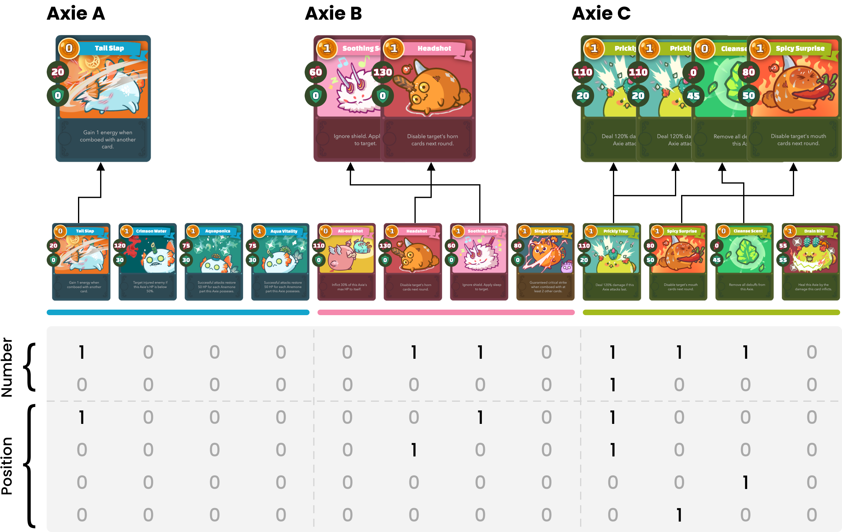
Figure 1: A demonstration of an encoded action consisting of 3 card sequences. Axie A/B/C respectively places 1/2/4 cards in this round. The status of each card is encoded in a 6-digit vector where the first two digits represent the number of this card and the rest 4 digits encode its positional information. The matrix is formed by 12 such vectors for 12 distinct cards.

We define the reward as the result of the game, with a penalty on the activity discarding cards. Mathematically, we denote the terminal state set $\mathcal{T}$ as a set of states at which the game is over. For a transition tuple $(s_{t},a_{t},s_{t+1})$, $0\leq t<T-1$, we define the reward function as

$$r_{t}(s_{t},a_{t},s_{t+1})=\begin{cases}I-c\cdot n_{d},&\text{if }s_{t+1}\in\mathcal{T},\\ 0,&o.w.,\end{cases}$$

where $I$ and $n_{d}$ are components in $s_{t+1}$. The game result indicator $I$ equals to 1/0/-1 if the agent wins/ties/loses the game, and $n_{d}$ is the number of discarded cards in the whole game. The positive constant $c$ adjusts the importance of the penalty term.

III Methodology

Due to the challenges brought by the large-scale action space, we consider to only evaluate a small group of actions which are filtered out from all feasible actions. We form this small set of actions with those actions which have similar effects with a target action. This target action is generated by a policy function. A distance function is needed to measure the “similarity” between two actions. Inspired by Word2Vec [14], we learn an action embedding function which maps one-hot-like action vectors into a continuous space which is defined as the latent action space. The Euclidean distance in this latent space reflects the difference between two actions in terms of their effects.

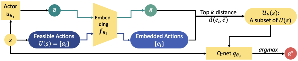
Figure 2: An illustration on the decision procedure.

III-A A Decision Procedure

We illustrate the decision procedure in Figure 2. This decision procedure of our method consists of 3 parametrized components:

1. A raw policy function $u_{\theta_{1}}:\mathcal{S}\rightarrow\mathbb{R}^{n}$ where $n$ is the dimensions of the action space, $\mathcal{A}\subset\mathbb{R}^{n}$.

2. An embedding function $f_{\theta_{2}}:\mathbb{R}^{n}\rightarrow\mathcal{E}$ where $\mathcal{E}$ is the latent action space, and $\mathcal{E}\subset\mathbb{R}^{m}$, $m<n$. For an arbitrary action $a$, $e=f_{\theta_{2}}(a)$ is called the latent action representation of $a$.

3. A state-action value function, i.e., a Q-function $q_{\theta_{3}}:\mathcal{S}\times\mathcal{A}\rightarrow\mathbb{R}$. The Q-value $q_{\theta_{3}}(s,a)$ evaluates the expected return when executing action $a$ at state $s$.

For a given input $s$, the overall policy function $\mu$ selects the action using the following procedure. Firstly, we obtain a point $\bar{a}=u_{\theta_{1}}(s)$ as a “raw action”, note it is possible that $\bar{a}\not\in\mathcal{A}$. Secondly, we denote the set of all available actions for $s$ as $U(s)$. We calculate the distance between available actions with the raw action in the latent space by $d(a,\bar{a};f_{\theta_{2}})=\|f_{\theta_{2}}(a)-f_{\theta_{2}}(\bar{a})\|^{2}$ for all $a\in U(s)$. We form a $k$-element subset of $U(s)$ with the top $k$ closest actions to the raw action in the latent space, denote it as $\mathcal{U}_{k}(s;\theta_{1},\theta_{2})$. Mathematically, this is done by

$$\mathcal{U}_{k}(s;\theta_{1},\theta_{2})=\operatorname*{arg\,min}_{\mathcal{U}\subset U(s),|\mathcal{U}|=k}\sum_{a\in\mathcal{U}}d(a,u_{\theta_{1}}(s);f_{\theta_{2}}).$$ (1)

In the last, we select the action which has the highest Q-value in this subset. If we denote an overall policy function as $\mu$ for a given state $s$, the action is selected by

$$a^{*}=\mu(s;\theta_{1},\theta_{2},\theta_{3})=\operatorname*{arg\,max}_{a\in\mathcal{U}_{k}(s;\theta_{1},\theta_{2})}q_{\theta_{3}}(s,a).$$ (2)

III-B Training procedures

Our method consists of three sets of parameters $\theta_{1}$, $\theta_{2}$, and $\theta_{3}$. We design a two-stage algorithm to train these parameters.

In the first stage of training, we design a supervised learning method to learn the embedding function $f_{\theta_{2}}$. We learn the action representations based on the effects of the actions on the system states. For instance, assume an arbitrary state $s\in\mathcal{S}$ and two actions $a_{1}$ and $a_{2}$, if the probability measure $p(s,a_{1})$ is similar to $p(s,a_{2})$ where $p(s,a)=P(S_{t+1}\mid S_{t}=s,A_{t}=a)$, we say $a_{1}$ and $a_{2}$ have similar effects. Following this idea, we train the embedding function by learning a model of the system dynamics which consists of the embedding function $f_{\theta_{2}}$. We illustrate the architecture of the system model in Figure 3. Specifically, we define a deterministic transition function $m_{\theta_{4}}:\mathcal{S}\times\mathcal{\mathcal{E}}\rightarrow\mathcal{S}$, which maps the state and action embedding to the next state. Thus, $m_{\theta_{4}}(s,f_{\theta_{2}}(a))$ should estimate the next state after executing $a$ at $s$. We define the following objective function to minimize the mean square error between the estimated next states with the actual next states

$$J_{1}(\theta_{2},\theta_{4})=\mathbb{E}_{P_{t},\cdot}[(m_{\theta_{4}}(s,f_{\theta_{2}}(a))-s^{\prime})^{2}].$$ (3)

We collect the transition tuples $(s,a,s^{\prime})$ in a dataset $D$ by randomly selecting actions. Then, we apply a gradient-based optimization method to optimize $\theta_{2}$ and $\theta_{4}$ by minimizing $J_{1}$ on $D$. In the next stage of training, we discard the dense layers, and only use the embedding function $\theta_{2}$.

In the second stage of training, similar to Deep Deterministic Policy Gradient in [2], we apply an iterative training procedure to alternatively update the deterministic raw policy function (the actor) $u_{\theta_{1}}$ and the Q-function (the critic) $q_{\theta_{3}}$. We use the raw action $\bar{a}$ instead of the final action $a^{*}$ in the policy improvement part [11]. The Q-function training uses Monte-Carlo estimate described in [15].

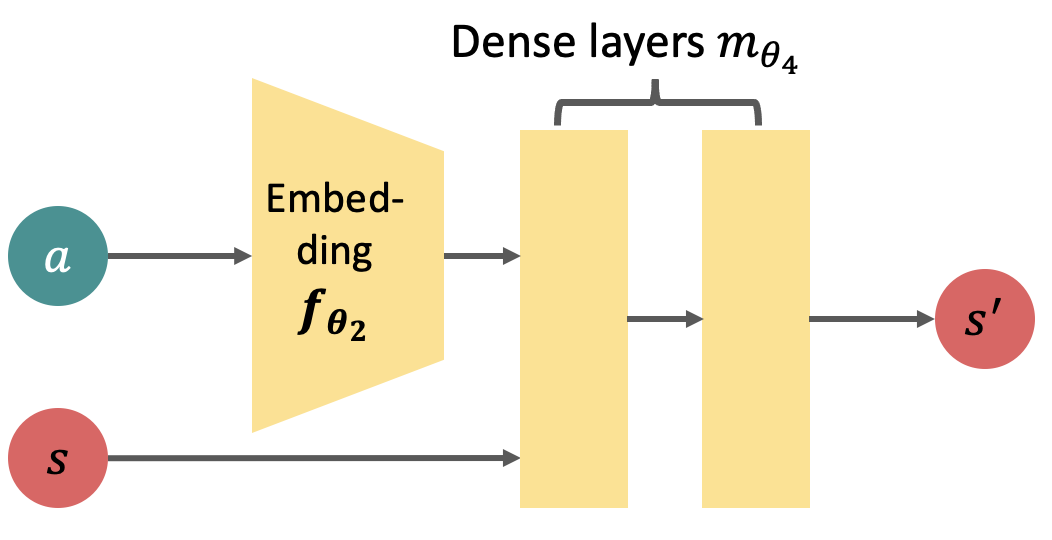
Figure 3: An illustration of the model of the system dynamics.

IV Experiment

In this section, we compare our method with two baseline methods:

1. DouZero. We adapt the DouZero method in [5] to our problem. We design a similar action encoding scheme as the one mentioned in this paper, where each action is encoded as a 2-by-12 matrix.

2. DouZero+pooling. We reduce the size of the action space by shrinking its dimensions. We design this baseline method by adding an 1D pooling layer [16] on the flattened actions from DouZero.

Indeed, other techniques to reduce the scale of action spaces are mentioned in [13]. They inevitably introduce prior human knowledge, which conflicts with our intention, and this makes the comparison unfair. In our experiments, we try to answer the following questions:

1. Does our method produces overall better performance than other baseline methods?

2. Does our method achieve better sample efficiency?

IV-A Sample Efficiency

We select six teams that are popular at different levels in the global rank. A detailed description of these teams can be found in Appendix VI-B. We train a model for each team using 3 methods: our method, the DouZero method, and the DouZero+pooling method. Thus, we trained 18 models in total. To make a fair comparison, we stop the training after $1\times 10^{7}$ steps for all these models.

Figure 4 shows the evolution of average returns during training in the first $1\times 10^{5}$ steps. It can be seen that, on most of the teams, the models from our method have the highest average return among the three by trained with the same amount of samples. This indicates that our method can quickly produce high-quality models due to high sample efficiency.

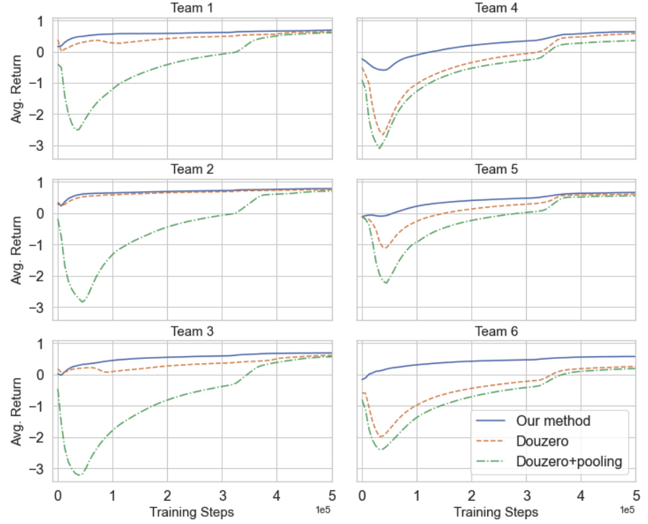
Figure 4: Comparison on the learning curves. Six line-charts shows the learning curves of 18 models in the first $5\times 10^{5}$ steps. It can be seen that our method shows a faster convergence with the same amount of samples on most of the 6 teams.

IV-B Battle

We evaluate the performance of each model by letting it play against other models and rule-based players. This guarantees that the models trained for the same team have the same set of opponents. Each battle consists of 1000 games. Each model plays 29000 games against various opponents to obtain a comprehensive result. This makes the variance of estimators of the winning rates small enough to show statistical significance.

We aggregate the winning rate of the models trained by each method in Table I. It can be seen that the overall winning rate of our method is 5% and 7% higher than the DouZero and DouZero+pooling method respectively. This also confirms our method has a better generalization ability on different teams.

TABLE I: The average wining rate of 3 methods on 6 teams
(174000 games for each method)

Method Winning rate Our method 0.4986 DouZero 0.4477 DouZero+pooling 0.4283

We also compare the models which use the same team. For each team, we calculate the difference between the number of wins by our method with that of DouZero or DouZero+pooling. A positive difference indicates our method plays this team better than the baseline method. We visualize these differences in the number of wins in Figure 5. We can find that our method can achieve a higher number of wins across most teams than the baseline methods. This indicates that our method has good generalizability to most team types. We notice that our method cannot outperform DouZero on teams 2 and 6. The reason is that strategies for these two teams are more diversified than those for the other teams. This makes high-reward actions far away from each other in the latent space. In such cases, the DouZero method may make better decisions than our method because it evaluates every feasible actions, though it is more computationally expensive.

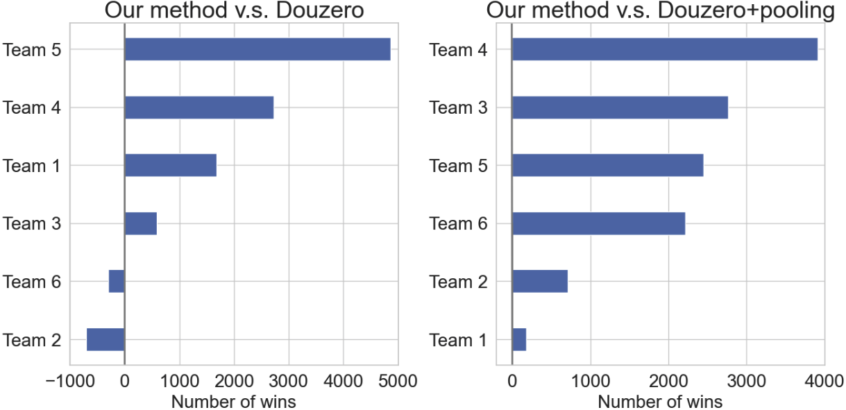
Figure 5: Comparison on battle performance between our method with two baseline methods on 6 teams. We train 18 models using these three methods on 6 teams. We evaluate each model by letting it play against a same set of opponent players consisting of the other trained agents and random players (29000 battles in total). Note the qualities in the left/right bar-plot respectively show (the number of wins of our method - the number of wins of the DouZero/DouZero+pooling method).

IV-C Time of Action Selections

Axie Infinity requires players to make decisions in 30 seconds in every round. We mention that some methods such as Monte Carlo Tree Search (MCTS) in [17] can also achieve good performance, but they usually fail to select cards by the time limit. We show our method is more efficient in time than the other two baseline methods using the time consumed by selecting card sequences. We test the 18 models in 1000 rounds, and record the time for selecting cards. Table II shows the statistics of the distribution of time for card selections for three methods. It can be seen that our method uses shorter time than the other two methods in average. The 25% quantiles for the three methods are similar, but the 75% quantiles of the two baseline methods is mush higher than that of our method. This indicates that our method has more consistent performance in terms of the time. This confirms that our method benefits from only evaluating actions in a fixed-size subset from all feasible actions.

TABLE II: The distribution of time for selecting cards by three methods (in millisecond)

Statistics Our Method DouZero DouZero+pooling Mean 7.42 18.71 16.35 Std 18.42 86.67 72.28 25% Quantile 5.01 4.91 5.22 50% Quantile 5.64 8.71 8.61 75% Quantile 7.00 16.50 15.87 Max 1186.32 3699.20 3707.82

V Conclusions

In this study, we try to use an RL method to solve the challenges in a card game problem with a large action space. We give the MDP formulation for the game Axie Infinity. We propose a general RL algorithm to learn the strategies of different teams. We design a training procedure to learn the action embedding function without prior information. We empirically demonstrate our method outperforms the baseline methods in terms of the battle performance and the sample efficiency.

Our work can be improved by incorporating the self-play technique [17] in training to enhance the opponents. Moreover, learning prior information from the textual data of card descriptions can enhance the action embedding component in our method. Future works may focus on this direction for further improvement.

VI Appendix

VI-A Game rules

We briefly explain the rules of Axie Infinity in this section. More detailed rules can be found in the website (https://whitepaper.axieinfinity.com/).

Axie Infinity is an online one-verse-one card game. Axies are virtual pets in this game, and they can be traded between players. Figure 6 illustrates the attributes of an Axie. The behavior of an Axie can be determined by three of its characteristics: the class, the attributes (stats), and the cards. The game has 9 classes in total. Every class is stronger than three classes, and is weaker to other three classes. Figure 7 depicts the relationship between 9 classes. In battles, an Axie produces more/less damages to other Axies if their class are weak/strong against the class of this Axie. Attributes (stats) consist of 4 values which indicate the Axie’s ability in Health/Speed/Skill/Morale. Every Axie carries 8 cards – 2 copies of 4 distinct cards. Players need to buy three Axies to form a team for combat. Thus, this forms a 24-card deck for the player to play.

Figure 8 demonstrates a battle between two players. Two players play cards round by round. In each round, the player draws cards from the card deck and gains energy points. The energy points limit the number of cards to select since some cards need energy points to execute. Most of the cards consume 0 or 1 energy point. The player can select at most 4 cards from an Axie, the order of these 4 cards can significantly impact their effects. Thus, the player create 3 card sequences from each Axie to play in a round. Once the card sequences are determined, the player can hit “End Turn” button, and the card sequences submitted by the two players are executed in an order which is associated with the Axies’ attributes and the card effects. The cards produce damages to the Axies on the other side. Each Axie has health points, the Axie is beaten when it has 0 health point. When all three Axies on a side are beaten, the game ends, and the player whose at least one Axie is alive wins this game. If all six Axies are beaten, a tie is reached. If the game can continue after the card execution, next round starts and the players draw cards from the remaining card deck again. Once the card deck is exhausted, the used cards are automatically shuffled and form a new card deck.

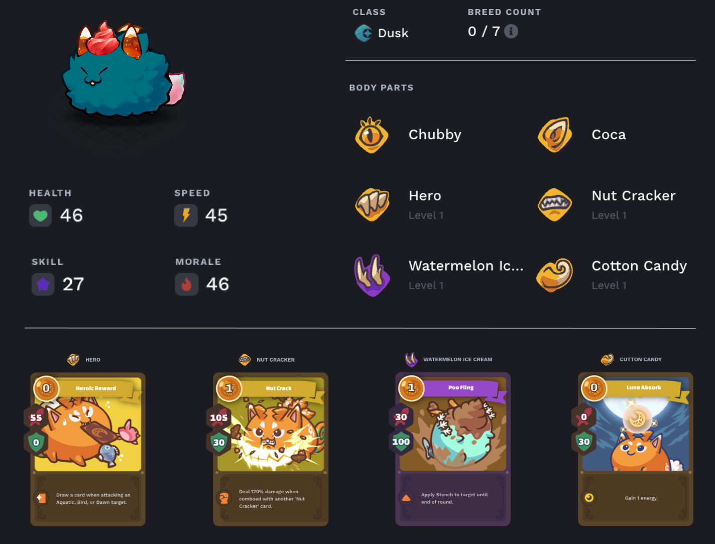
Figure 6: An illustration of the attributes of an Axie.

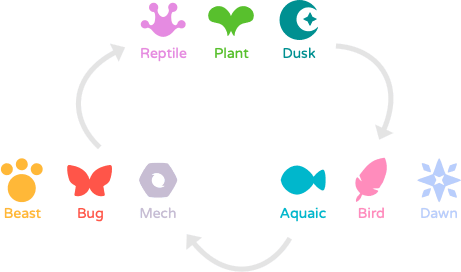
Figure 7: The relationship between the 9 classes.

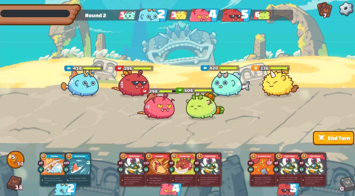
Figure 8: A snapshot of a battle of Axie Infinity.

VI-B Teams in the experiments

In order to validate our method, we select six teams which are popular from different levels in the global rank. Since the human strategies for these six teams are very different, our method ideally can lean these diversified strategies. The following tables show the detailed information for the 6 teams in our experiments.

TABLE III: Details of the Six teams in the experiments

Team 1 Axie 1 Axie 2 Axie 3 Axie Class Aquatic Plant Bird Axie Stats 45/57/35/27 61/31/31/41 27/59/35/43 Axie Card 1 Aqua Vitality Cleanse Scent Single Combat Axie Card 2 Crimson Water Drain Bite Soothing Song Axie Card 3 Aquaponics Prickly Trap Headshot Axie Card 4 Tail Slap Spicy Surprise All-out Shot

Team 2 Axie 1 Axie 2 Axie 3 Axie Class Aquatic Bug Dusk Axie Stats 45/51/35/33 43/35/35/51 57/41/27/39 Axie Card 1 Swift Escape Scarab Curse Ivory Chop Axie Card 2 Terror Chomp Terror Chomp Terror Chomp Axie Card 3 Bug Signal Bug Signal Bug Signal Axie Card 4 Tail Slap Anesthetic Bait Cattail Slap

Team 3 Axie 1 Axie 2 Axie 3 Axie Class Plant Dusk Mech Axie Stats 56/33/31/44 59/47/27/31 37/48/43/36 Axie Card 1 October Treat Ivory Chop Juggling Balls Axie Card 2 Vegetal Bite Sneaky Raid Sneaky Raid Axie Card 3 Disguise Surprise Invasion Sinister Strike Axie Card 4 Gas Unleash Venom Spray Twin Needle

Team 4 Axie 1 Axie 2 Axie 3 Axie Class Plant Dusk Dusk Axie Stats 59/31/31/43 57/43/27/37 51/50/27/36 Axie Card 1 October Treat Barb Strike Barb Strike Axie Card 2 Vegetal Bite Sneaky Raid Chomp Axie Card 3 Disguise Surprise Invasion Smart Shot Axie Card 4 Gas Unleash Venom Spray Venom Spray

Team 5 Axie 1 Axie 2 Axie 3 Axie Class Plant Dusk Dusk Axie Stats 59/31/31/43 54/48/27/35 51/46/27/40 Axie Card 1 October Treat Spike Throw Sticky Goo Axie Card 2 Vegetal Bite Chomp Chomp Axie Card 3 Disguise Disarm Mystic Rush Axie Card 4 Gas Unleash Allergic Reaction Allergic Reaction

Team 6 Axie 1 Axie 2 Axie 3 Axie Class Plant Beast Bird Axie Stats 59/31/31/43 32/45/31/56 27/61/35/41 Axie Card 1 October Treat Single Combat Blackmail Axie Card 2 Vegetal Bite Nut Crack Dark Swoop Axie Card 3 Disguise Nut Throw Eggbomb Axie Card 4 Carrot Hammer Ivory Stab All-out Shot

References

- [1] V. Mnih, K. Kavukcuoglu, D. Silver, A. A. Rusu, J. Veness, M. G. Bellemare, A. Graves, M. Riedmiller, A. K. Fidjeland, G. Ostrovski et al., “Human-level control through deep reinforcement learning,” nature, vol. 518, no. 7540, pp. 529–533, 2015.
- [2] T. P. Lillicrap, J. J. Hunt, A. Pritzel, N. Heess, T. Erez, Y. Tassa, D. Silver, and D. Wierstra, “Continuous control with deep reinforcement learning,” arXiv preprint arXiv:1509.02971, 2015.
- [3] V. Mnih, A. P. Badia, M. Mirza, A. Graves, T. Lillicrap, T. Harley, D. Silver, and K. Kavukcuoglu, “Asynchronous methods for deep reinforcement learning,” in International conference on machine learning. PMLR, 2016, pp. 1928–1937.
- [4] J. Schulman, F. Wolski, P. Dhariwal, A. Radford, and O. Klimov, “Proximal policy optimization algorithms,” arXiv preprint arXiv:1707.06347, 2017.
- [5] D. Zha, J. Xie, W. Ma, S. Zhang, X. Lian, X. Hu, and J. Liu, “Douzero: Mastering doudizhu with self-play deep reinforcement learning,” in International Conference on Machine Learning. PMLR, 2021, pp. 12 333–12 344.
- [6] M. Bowling, N. Burch, M. Johanson, and O. Tammelin, “Heads-up limit hold’em poker is solved,” Science, vol. 347, no. 6218, pp. 145–149, 2015.
- [7] N. Brown and T. Sandholm, “Superhuman ai for heads-up no-limit poker: Libratus beats top professionals,” Science, vol. 359, no. 6374, pp. 418–424, 2018.
- [8] ——, “Superhuman ai for multiplayer poker,” Science, vol. 365, no. 6456, pp. 885–890, 2019.
- [9] J. Li, S. Koyamada, Q. Ye, G. Liu, C. Wang, R. Yang, L. Zhao, T. Qin, T.-Y. Liu, and H.-W. Hon, “Suphx: Mastering mahjong with deep reinforcement learning,” arXiv preprint arXiv:2003.13590, 2020.
- [10] Y. Guan, M. Liu, W. Hong, W. Zhang, F. Fang, G. Zeng, and Y. Lin, “Perfectdou: Dominating doudizhu with perfect information distillation,” arXiv preprint arXiv:2203.16406, 2022.
- [11] G. Dulac-Arnold, R. Evans, H. van Hasselt, P. Sunehag, T. Lillicrap, J. Hunt, T. Mann, T. Weber, T. Degris, and B. Coppin, “Deep reinforcement learning in large discrete action spaces,” arXiv preprint arXiv:1512.07679, 2015.
- [12] Y. Chandak, G. Theocharous, J. Kostas, S. Jordan, and P. Thomas, “Learning action representations for reinforcement learning,” in International conference on machine learning. PMLR, 2019, pp. 941–950.
- [13] A. Kanervisto, C. Scheller, and V. Hautamäki, “Action space shaping in deep reinforcement learning,” in 2020 IEEE Conference on Games (CoG). IEEE, 2020, pp. 479–486.
- [14] T. Mikolov, K. Chen, G. Corrado, and J. Dean, “Efficient estimation of word representations in vector space,” arXiv preprint arXiv:1301.3781, 2013.
- [15] R. S. Sutton and A. G. Barto, Reinforcement learning: An introduction. MIT press, 2018.
- [16] D. Yu, H. Wang, P. Chen, and Z. Wei, “Mixed pooling for convolutional neural networks,” in International conference on rough sets and knowledge technology. Springer, 2014, pp. 364–375.
- [17] D. Silver, T. Hubert, J. Schrittwieser, I. Antonoglou, M. Lai, A. Guez, M. Lanctot, L. Sifre, D. Kumaran, T. Graepel et al., “A general reinforcement learning algorithm that masters chess, shogi, and go through self-play,” Science, vol. 362, no. 6419, pp. 1140–1144, 2018.