A SIQRB delayed model for cholera and optimal control treatment

Abstract.

We improve a recent mathematical model for cholera by adding a time delay that represents the time between the instant at which an individual becomes infected and the instant at which he begins to have symptoms of cholera disease. We prove that the delayed cholera model is biologically meaningful and analyze the local asymptotic stability of the equilibrium points for positive time delays. An optimal control problem is proposed and analyzed, where the goal is to obtain optimal treatment strategies, through quarantine, that minimize the number of infective individuals and the bacterial concentration, as well as treatment costs. Necessary optimality conditions are applied to the delayed optimal control problem, with a $L^{1}$ type cost functional. We show that the delayed cholera model fits better the cholera outbreak that occurred in the Department of Artibonite – Haiti, from 1 November 2010 to 1 May 2011, than the non-delayed model. Considering the data of the cholera outbreak in Haiti, we solve numerically the delayed optimal control problem and propose solutions for the outbreak control and eradication.

1. Introduction

Cholera is an acute diarrheal infectious disease caused by infection of the intestine with the bacterium Vibrio cholerae, which lives in an aquatic organism. There are 200 serogroups of the bacterium Vibrio cholerae, but only two of them (O1 and O139) are responsible for the cholera disease [1, 2]. They pass through and survive the gastric acid barrier of the stomach and then penetrate the mucus lining that coats the intestinal epithelial [1, 3]. They colonize the intestine and then produce enterotoxin, which stimulates water and electrolyte secretion by the endothelial cells of the small intestine [1]. The ingestion of contaminated food or water can cause cholera outbreaks, as proved by John Snow in 1854 [4]. Nevertheless, there are other ways of spreading. Susceptible individuals can also become infected if they contact with infectious individuals. If these individuals are at an increased risk of infection, they can transmit the disease to other people that live with them and are involved in food preparation or use water storage containers, see e.g. [4]. An individual can be infective with or without symptoms which can appear from a few hours to 5 days, after infection. However, symptoms typically appear in 2–3 days: see [5]. Some symptoms are vomiting, leg cramps and copious, painless, and watery diarrhea. It is very important that infective individuals can get treatment as soon as possible, because without it they become dehydrated and they can suffer from acidosis and have a circulatory collapse. Even worse, this situation can lead to death within 12 to 24 hours [4, 6]. Some studies and experiments suggest that a recovered individual can be immune to the disease during a period of 3 to 10 years. On the other hand, recent researches suggest that immunity can be lost after a period of weeks to months [4, 7]. Diseases involving diarrhea are the major cause of child mortality in developing countries, because the access to clean drinking water and sanitation is difficult [8]. Moreover, Sun et al. wrote in [9] that this disease has generated a great threat to human society and caused enormous morbidity and mortality with weak surveillance system. Thus, it is very important to study mathematical models of the cholera spread in order to know how to curtail it.

Several mathematical models for the spread of cholera have been studied since, at least, 1979: see, e.g., [4, 6, 7, 10, 11, 12, 13, 14, 15, 16, 17, 18, 19, 20, 21, 22] and references cited therein. In [7], a SIR (Susceptible–Infectious–Recovered) type model is proposed, which considers two classes for the bacterial concentrations (hyper-infectious and less-infectious) and two classes for the infective individuals (asymptomatic and symptomatic). The authors compare a cost-effective balance of multiple intervention methods of two endemic populations, using optimal control theory, parameter sensitivity analysis, and numerical simulations. Wang and Modnak [21] also consider a SIR type model with a class for the Vibrio cholerae concentration in the environment. The model incorporates three control measures: vaccination, therapeutic treatment, and water sanitation. The stability analysis of equilibrium points is done when the controls are given by constant values. They also study a more general cholera model with time-dependent controls, proving existence of solution to an optimal control problem and deriving necessary optimality conditions based on Pontryagin’s Maximum Principle. The authors of [6] incorporate in a SIR type model public health educational campaigns, vaccination, quarantine, and treatment, as control strategies. The model also considers a class for the bacterial concentration. The education-induced, vaccination-induced, and treatment-induced reproductive numbers, as well as the combined reproductive number, are compared with the basic reproduction number to assess the possible community benefits of these strategies. The stability analysis of the equilibria is performed using a Lyapunov functional approach. In [4], a SIR type model with distributed delays is proposed. It incorporates hyperinfectivity, where infectivity varies with the time since the pathogen was shed, and temporary immunity. The basic reproduction number is computed and it plays an important role to know if the disease dies out or not. Numerical simulations are carried out in order to illustrate important details of the unique endemic equilibrium’s stability. In [23], Wang and Liao present a SIR type model with a class for the Vibrio cholerae concentration in the contaminated water. It is an unified deterministic model for cholera, because it considers a general incidence rate and a general formulation of the pathogen concentration. The basic reproduction number is computed and conditions are derived for the existence of the disease-free and endemic equilibrium points. The local asymptotic and global stability analysis of the equilibrium points are studied. The authors show that different models can be studied in a single framework, using three representative cholera models presented in [12, 13, 24]. A mathematical model that considers public health educational campaigns, vaccination, sanitation, and treatment as control strategies, is formulated in [25]. The reproduction number for the cases with single and combined controls is determined and compared. The authors conclude that, when one considers a single control measure, treatment yields the best results, followed by education campaigns, sanitation, and vaccination; cf. the numerical simulations of [25]. Nevertheless, the more control strategies are considered, better results can be obtained. Furthermore, the authors perform a sensitivity analysis on the key parameters that drive the disease dynamics in order to find their relative importance to cholera’s spread and prevalence. In [8], a SIR type model with a class for the bacterial concentration in the environment is proposed, which incorporates media coverage. The existence and stability of the equilibria is analyzed. Numerical simulations suggest that the number of infections decreases faster, when media coverage is very efficient. So, media alert and awareness campaigns are crucial for controlling the spread of cholera. In [9], a SIR type mathematical model for cholera transmission is used to characterize the cholera spread in China. With the purpose of avoiding cholera outbreaks in China, the researchers suggest to increase the immunization coverage rate and to make efforts for improving environmental management, mainly for drinking water [9]. Another important topic to have a full overview of mathematical modeling, within the scope of SIR models in biomathematics, concerns uncertainty quantification using randomized models, as, e.g., in [26, 27]. With respect to cholera, one can find, e.g., the paper [22], where the authors propose and analyze a stochastic epidemic model to study such disease.

The worst cholera outbreak in human history has occurred in Yemen and it has provoked 1 115 378 suspected cholera cases and 2 310 deaths, from 27 April 2017 to 1 July 2018 [28]. In [19], the authors forecast this cholera epidemic, explicitly addressing the reporting delay and ascertainment bias (see also [18]). The Yemen outbreak data available in the website of World Health Organization is also fitted by He et al. in [29], considering a mathematical model based on differential equations. Their model considers five classes: $S$ (susceptible individuals), $I$ (infectious individuals), $R$ (recovered individuals), $B$ (concentration of bacterium in the environment), and $M$ (availability of medical resources in the country). Such model translates the interaction between the human hosts and the pathogenic bacteria, under the impact of limited medical resources. The results obtained in [29] support that improvement of the public health system and strategic implementation of control measures with respect to time and location can facilitate the prevention and intervention related to this disease in Yemen. In [30], a SITRV (Susceptible–Infectious–Treated–Vaccinated–Recovered) type model with a class for bacterial concentration is proposed and mathematically studied. The cholera outbreak in Yemen is numerically simulated through a sub-model of the model mentioned previously. Moreover, a numerical simulation, which considers an hypothetical situation with vaccination since the beginning of the epidemic, is carried out. The obtained results support the importance of vaccination to prevent cholera spread.

Cholera is one of the international quarantine infectious diseases, as stipulated by the International Health Regulations (IHR) [1]. In agreement with this fact, in [16] a SIQR (Susceptible–Infectious–Quarantined–Recovered) type model is proposed and analyzed. In [16] it is assumed that infective individuals are subject to quarantine during the treatment period. As the symptoms of the disease can not appear immediately after the infection (see [5]), we propose here an improvement of the work done in [16], by considering and analyzing a delayed SIQR type model. More precisely, we introduce a discrete time-delay that represents the time between the instant at which an individual becomes infected and the instant at which he begins to have symptoms of cholera.

Several cholera outbreaks have occurred since 2007, namely in Angola, Haiti, Zimbabwe, and Yemen [4, 31]. In Haiti, the first cases of cholera happened in the Department of Artibonite on 14th October 2010. The disease spread along the Artibonite river and reached several departments. Only within one month, all departments had reported cases in rural areas and places without good conditions of public health [32]. We provide numerical simulations for the cholera outbreak in the Department of Artibonite, from 1 November 2010 to 1 May 2011 [32], improving the results in [16].

We propose and analyze an optimal control problem with a state delay, where the control function represents the fraction of infective individuals $I$ that will be submitted to treatment in quarantine until complete recovery. The objective is to find the optimal treatment strategy through quarantine that minimizes the number of infective individuals and the bacterial concentration, as well as the cost of interventions associated with quarantine. We apply the Pontryagin Minimum Principle for time-delayed optimal control problems (see [33, 34]) with $L^{1}$-type cost functional. The delayed and non-delayed optimal control problems with $L^{1}$ cost functionals are analyzed, analytically and numerically, the solutions being interpreted from an epidemiological point of view.

The paper is organized as follows. In Section 2, we propose a delayed model for the cholera transmission dynamics. In Section 3, the delayed model is analyzed, proving the non-negativity of the solutions for non-negative initial conditions and providing the disease-free equilibrium, basic reproduction number $R_{0}$, and endemic equilibrium, when $R_{0}>1$. The stability of the equilibrium points is analyzed for positive time delays. Concretely, a stability analysis of the endemic equilibrium, as function of the ingestion rate of the bacteria through contaminated sources, is carried out. In Section 4, we consider the cholera outbreak that occurred in the Department of Artibonite – Haiti, from 1 November 2010 to 1 May 2011 [32], improving the numerical simulations done in [16] by considering a positive time delay, treatment, and recovery. In Section 5, we formulate a SIQRB (Susceptible–Infectious–Quarantined–Recovered–Bacterial) time-delayed optimal control problem with $L^{1}$ cost functional. Necessary optimality conditions are discussed. We consider different delayed control problems and compute extremal solutions using discretization and nonlinear programming methods. Section 6 presents our main conclusions.

2. Model formulation

We revisit the dynamic model studied in [16] and introduce a time delay $\tau\geq 0$, which represents the time between the instant in which an individual becomes infected and the instant in which he begins to show symptoms. Thus, we propose a time-delayed model that involves a SIQR (Susceptible–Infectious–Quarantined–Recovered) system and that also considers a class of bacterial concentration in the dynamics of cholera. The total population $N(t)$ is divided into four classes: susceptible $S(t)$, infectious with symptoms $I(t)$, in treatment through quarantine $Q(t)$, and recovered $R(t)$ at time $t$, for $t\geq 0$. Furthermore, the class $B(t)$ reflects the bacterial concentration at time $t\geq 0$. The time delay $\tau\geq 0$ is related with the passage of individuals from class $S$ to class $I$. The introduction of this delay is done with the goal to better approximate reality. The symptoms of cholera can appear from a few hours to 5 days after infection. Nevertheless, they typically appear in 2–3 days [5]. We assume that there is a positive recruitment rate $\Lambda$ into the susceptible class $S(t)$ and a constant natural death rate $\mu>0$. Susceptible individuals can become infected with cholera at rate $\displaystyle\frac{\beta B(t)}{\kappa+B(t)}$ that is dependent on time $t$. Note that $\beta>0$ is the ingestion rate of the bacteria through contaminated sources, $\kappa$ is the half saturation constant of the bacteria population, and $\displaystyle\frac{B(t)}{\kappa+B(t)}$ is the likeliness of an infective individual to have the disease with symptoms, given a contact with contaminated sources [6]. Any recovered individual can loose the immunity at rate $\omega$ and therefore becomes susceptible again. The infective individuals can accept to be in quarantine during a period of time. During this time they are isolated and subject to a proper medication, at rate $\delta$. The quarantined individuals can recover at rate $\varepsilon$. The disease-related death rates associated with the individuals that are infective and in quarantine are $\alpha_{1}$ and $\alpha_{2}$, respectively. Each infective individual contributes to the increase of the bacterial concentration at rate $\eta$. On the other hand, the bacterial concentration can decrease at mortality rate $d$. These assumptions are translated into the following mathematical model:

$$\begin{cases}\begin{split}\dot{S}(t)&=\Lambda-\displaystyle\frac{\beta B(t)}{\kappa+B(t)}S(t)+\omega R(t)-\mu S(t),\\[4.26773pt] \dot{I}(t)&=\displaystyle\frac{\beta B(t-\tau)}{\kappa+B(t-\tau)}S(t-\tau)-(\delta+\alpha_{1}+\mu)I(t),\\[4.26773pt] \dot{Q}(t)&=\delta I(t)-(\varepsilon+\alpha_{2}+\mu)Q(t),\\[4.26773pt] \dot{R}(t)&=\varepsilon Q(t)-(\omega+\mu)R(t),\\[4.26773pt] \dot{B}(t)&=\eta I(t)-dB(t).\\[2.84544pt] \end{split}\end{cases}$$ (1)

In Figure 1, the model (1) is presented in a schematic way.

Note that

1. the parameters $\Lambda$, $\mu$, $\beta$, $\kappa$, $\eta$, and $d$ are strictly positive while $\omega$, $\delta$, $\varepsilon$, $\alpha_{1}$, $\alpha_{2}$, and $\tau$ are nonnegative.

2. individuals in class $R$ have already finalized their treatment, being recovered and, consequently, immune to cholera. Following [1, 4, 6, 8], we assume that there is no cholera induced-deaths for recovered individuals. In this way, it makes sense to consider that both susceptible and recovered individuals die at natural death rate $\mu$. In other words, we are considering that only non-treated infectious individuals with symptoms, or in treatment, can die due to cholera.

Figure 1. Diagram of the dynamical model (1).

3. Model analysis

First, we prove that the model (1) makes sense from a biological point of view, because the solutions of (1) are non-negative under non-negative initial conditions. Secondly, we give the expressions of the disease-free and endemic equilibrium points, as well as the expression of the basic reproduction number. Then, we proceed with the linearization of the model, which allows to derive some important results needed in the stability study of the equilibria. In the sequel, we shall consider the following notations:

1. $a_{1}=\delta+\alpha_{1}+\mu$;

2. $a_{2}=\varepsilon+\alpha_{2}+\mu$;

3. $a_{3}=\omega+\mu$;

4. $\rho=\Lambda\eta a_{2}a_{3}+\kappa d(a_{1}a_{2}a_{3}-\delta\varepsilon\omega)$;

5. $\bar{D}=a_{1}a_{2}a_{3}\mu+\beta(a_{1}a_{2}a_{3}-\delta\varepsilon\omega)$;

6. $A=a_{1}a_{2}a_{3}$;

7. $\tilde{A}=a_{1}a_{2}a_{3}-\delta\varepsilon\omega$.

3.1. Non-negativity of solutions

As in [16], we assume that the initial conditions of system (1) are non-negative:

$$S(t)=S_{0}\geq 0\,,\quad I(t)=I_{0}\geq 0\,,\quad Q(t)=Q_{0}\geq 0\,,\quad R(t)=R_{0}\geq 0\,\quad\text{and}\quad B(t)=B_{0}\geq 0\quad\text{ for all }\quad t\in[-\tau,0].$$ (2)

The model studied in [16] has biological meaning. Lemma 3.1 proves that the corresponding delayed model (1)–(2) also makes sense from the biological point of view.

One could consider suitable generic continuous functions for initial conditions (2). However, for the concrete situation of the Haiti outbreak under investigation, there is no way to know such continuous functions. For this reason, those continuous functions are here approximated by the constant functions (2).

The solutions $\left(S(t),I(t),Q(t),R(t),B(t)\right)$ of (1) are non-negative for all $t\geq-\tau$ with non-negative initial conditions (2).

Proof.

We have

$$\begin{cases}\begin{split}\frac{dS(t)}{dt}\bigg{|}_{\xi(S)}&=\ \Lambda+\omega R(t)>0\,,\\[4.26773pt] \frac{dI(t)}{dt}\bigg{|}_{\xi(I)}&=\ \displaystyle\frac{\beta B(t-\tau)S(t-\tau)}{\kappa+B(t-\tau)}\ \geq 0\,,\\[4.26773pt] \frac{dQ(t)}{dt}\bigg{|}_{\xi(Q)}&=\ \delta I(t)\ \geq 0\,,\\[4.26773pt] \frac{dR(t)}{dt}\bigg{|}_{\xi(R)}&=\ \varepsilon Q(t)\ \geq 0\,,\\[4.26773pt] \frac{dB(t)}{dt}\bigg{|}_{\xi(B)}&=\ \eta I(t)\ \geq 0\,,\end{split}\end{cases}$$

where $\xi(\upsilon)=\big{\{}\upsilon(t)=0\text{ and }S,I,Q,R,B\in C\big{(}[-\tau,+\infty[,\mathbb{R}_{0}^{+}\big{)}\big{\}}$ and $\upsilon\in\{S,I,Q,R,B\}$. Therefore, due to Lemma 2 in [35], any solution of system (1) is such that $\big{(}S(t),I(t),Q(t),R(t),B(t)\big{)}\in\big{(}\mathbb{R}_{0}^{+}\big{)}^{5}$ for all $t\geq-\tau$. ∎

3.2. Equilibrium points and the basic reproduction number

When a system of ordinary differential equations with constant parameters is in equilibrium, their states are represented by constant functions. In our case, in a state of equilibrium we have

$$\dot{S}(t)=\dot{I}(t)=\dot{Q}(t)=\dot{R}(t)=\dot{B}(t)=0.$$

Consequently, we get constant functions. Therefore, time delays do not affect the expressions of equilibria. Thus, equilibria of delayed and non-delayed $SIQRB$ models for cholera, with constant parameters, are the same. From [16], we know that model (1) has a disease-free equilibrium (DFE) given by

$$E^{0}=\big{(}S^{0},I^{0},Q^{0},R^{0},B^{0}\big{)}=\left(\frac{\Lambda}{\mu},0,0,0,0\right)$$ (3)

and that the basic reproduction number has the following expression:

$$R_{0}=\frac{\beta\Lambda\eta}{\mu\kappa da_{1}}.$$ (4)

Moreover, when $R_{0}>1$, there is an endemic equilibrium given by

$$E^{*}=(S^{*},I^{*},Q^{*},R^{*},B^{*}),$$ (5)

where

$$S^{*}=\displaystyle\frac{a_{1}\rho}{\eta\bar{D}},\quad I^{*}=\displaystyle\frac{\beta\Lambda a_{2}a_{3}(R_{0}-1)}{R_{0}\bar{D}},\quad Q^{*}=\displaystyle\frac{\beta\Lambda a_{3}\delta(R_{0}-1)}{R_{0}\bar{D}},\quad R^{*}=\displaystyle\frac{\beta\Lambda\delta\varepsilon(R_{0}-1)}{R_{0}\bar{D}},\quad B^{*}=\displaystyle\frac{\beta\Lambda\eta a_{2}a_{3}(R_{0}-1)}{R_{0}\bar{D}d}.$$

3.3. Linearisation of the model

Let us denote the state variables by $x_{1}=S$, $x_{2}=I$, $x_{3}=Q$, $x_{4}=R$ and $x_{5}=B$. Then, we can write the system (1) in the following way:

$$\dot{x}(t)=f\big{(}x(t),x(t-\tau)\big{)},$$

where $x=\big{(}x_{1},x_{2},x_{3},x_{4},x_{5}\big{)}$. Let $\bar{E}=(\bar{x}_{1},\bar{x}_{2},\bar{x}_{3},\bar{x}_{4},\bar{x}_{5})$ be an arbitrary equilibrium point of (1) and let us consider the following change of variables:

$$z_{i}(t)=x_{i}(t)-\bar{x}_{i},\quad i=1,\dots,5.$$

Thus, the linearized system of (1) is given by

$$\dot{z}=\frac{\partial f}{\partial x}\bigg{|}_{\bar{E}}z+\frac{\partial f}{\partial x_{\tau}}\bigg{|}_{\bar{E}}z_{\tau},$$

where $z(t)=\big{(}z_{1}(t),z_{2}(t),z_{3}(t),z_{4}(t),z_{5}(t)\big{)}$, $z_{\tau}(t)=z(t-\tau)$ and $x_{\tau}(t)=x(t-\tau)$. Furthermore, we have

$$A_{0}:=\frac{\partial f}{\partial x}\bigg{|}_{\bar{E}}=\left[\begin{matrix}-\bar{\lambda}-\mu&0&0&\omega&-C\\ 0&-a_{1}&0&0&0\\ 0&\delta&-a_{2}&0&0\\ 0&0&\varepsilon&-a_{3}&0\\ 0&\eta&0&0&-d\end{matrix}\right]$$

and

$$A_{1}:=\frac{\partial f}{\partial x_{\tau}}\bigg{|}_{\bar{E}}=\left[\begin{matrix}0&0&0&0&0\\ \bar{\lambda}&0&0&0&C\\ 0&0&0&0&0\\ 0&0&0&0&0\\ 0&0&0&0&0\end{matrix}\right],$$

where $\bar{\lambda}=\displaystyle\frac{\beta\bar{x}_{5}}{\kappa+\bar{x}_{5}}$ and $C=\displaystyle\frac{\beta\kappa\bar{x}_{1}}{(\kappa+\bar{x}_{5})^{2}}$. So, the characteristic polynomial associated with the linearized system of model (1) is given by

$$p_{\tau}(\chi)=\det(\chi I_{5}-A_{0}-e^{-\tau\chi}A_{1})=P_{1}(\chi)+e^{-\tau\chi}P_{2}(\chi),$$ (6)

where

$$P_{1}(\chi)=(\chi+a_{1})(\chi+a_{2})(\chi+a_{3})(\chi+d)(\chi+\bar{\lambda}+\mu)$$

and

$$P_{2}(\chi)=-\eta C\chi^{3}-\eta C(a_{2}+a_{3}+\mu)\chi^{2}-\Big{(}\eta C(a_{2}a_{3}+a_{2}\mu+a_{3}\mu)+\delta\varepsilon\omega\bar{\lambda}\Big{)}\chi-\eta Ca_{2}a_{3}\mu-\delta\varepsilon\omega d\bar{\lambda}.$$

3.4. Stability analysis

In order to study the stability of the equilibria, we are going to follow the approach of [36], corrected in [37] (see also Theorem 4.1 of [38, p. 83]). We shall prove that the conditions $(i)$, $(ii)$, $(iv)$ and $(v)$ of Theorem 4.1 of [38, p. 83] are satisfied for an arbitrary equilibrium point

$$\bar{E}=(\bar{x}_{1},\bar{x}_{2},\bar{x}_{3},\bar{x}_{4},\bar{x}_{5})\in(\mathbb{R}_{0}^{+})^{5}$$

of model (1). The polynomial $P_{1}$ has only real zeros ($\chi=-a_{1}$ or $\chi=-a_{2}$ or $\chi=-a_{3}$ or $\chi=-d$ or $\chi=-\bar{\lambda}-\mu$). Thus, the polynomials $P_{1}$ and $P_{2}$ can not have common imaginary zeros and condition $(i)$ is satisfied. In order to fulfill the hypothesis of condition $(ii)$, we are going to compute $P_{1}(yi)$ and $P_{2}(yi)$. We have

$$\begin{split}P_{1}(yi)&=\ \big{[}a_{1}(\bar{\lambda}+\mu)-y^{2}\big{]}\big{[}a_{2}a_{3}d-(a_{2}+a_{3}+d)y^{2}\big{]}-(a_{1}+\bar{\lambda}+\mu)\big{[}a_{2}a_{3}+(a_{2}+a_{3})d-y^{2}\big{]}y^{2}\\ &\quad+\Big{\{}\big{[}a_{1}(\bar{\lambda}+\mu)-y^{2}\big{]}\big{[}a_{2}a_{3}+(a_{2}+a_{3})d-y^{2}\big{]}+(a_{1}+\bar{\lambda}+\mu)\big{[}a_{2}a_{3}d-(a_{2}+a_{3}+d)y^{2}\big{]}\Big{\}}yi\\ &=\ \overline{P_{1}(-yi)}\end{split}$$

and one obtains that

$$\begin{split}P_{2}(yi)&=\eta C(a_{2}+a_{3}+\mu)y^{2}-\eta Ca_{2}a_{3}\mu-\delta\varepsilon\omega\bar{\lambda}d+\Big{\{}\eta Cy^{3}-\big{[}\eta C(a_{2}a_{3}+a_{2}\mu+a_{3}\mu)+\delta\varepsilon\omega\bar{\lambda}\big{]}y\Big{\}}i\\ &=\ \overline{P_{2}(-yi)}.\end{split}$$

Therefore, condition $(ii)$ is also satisfied. As the degree of polynomial $P_{1}$, equal to five, is bigger than the degree of $P_{2}$, equal to three, then the condition $(iv)$, given by

$$\lim\limits_{|\lambda|\rightarrow\infty,\ \Re(\lambda)\geq 0}\sup\left\{\left|\frac{P_{2}(\lambda)}{P_{1}(\lambda)}\right|\right\}<1,$$

is obviously satisfied. Furthermore, the function defined by $F(y)=|P_{1}(yi)|^{2}-|P_{2}(yi)|^{2}$ is a polynomial with degree equal to ten. Thus, the function $F$ has at most a finite number (ten) of real zeros. Concluding, the condition $(v)$ is also verified.

3.4.1. Disease-free equilibrium

Now, we are going to study the stability of the DFE (3) of the delayed model (1).

[Stability of the DFE (3)] Assume that $R_{0}\neq 1$. If $a_{1}d<1$, then there exists $\tau^{*}\in\mathbb{R}_{0}^{+}$ such that:

• there is at most a finite number of stability switches, when $\tau\in[0,\tau^{*}]$;

• instability occurs, when $\tau\in\,]\tau^{*},+\infty[$.

For all $\tau\geq 0$, if $a_{1}d\geq 1$, then the DFE (3) is:

• locally asymptotic stable, when $R_{0}<1$;

• unstable, when $R_{0}>1$.

Proof.

In order to study the stability of the DFE, we follow the approach of [36, 37]. We already know that the conditions $(i)$, $(ii)$, $(iv)$, and $(v)$ of Theorem 4.1 of [38, p. 83] are satisfied for the DFE. Thus, we analyze now the condition $(iii)$ and compute the zeros of the polynomial $F$ for the DFE. Computing $P_{1}(0)+P_{2}(0)$, we obtain

$$P_{1}(0)+P_{2}(0)=a_{1}a_{2}a_{3}d\mu-\eta Ca_{2}a_{3}\mu=a_{1}a_{2}a_{3}d\mu-a_{1}dR_{0}a_{2}a_{3}\mu=a_{1}a_{2}a_{3}d\mu(1-R_{0}).$$

Concluding, $P_{1}(0)+P_{2}(0)\neq 0\Leftrightarrow R_{0}\neq 1$, because $a_{1},a_{2},a_{3},d,\mu>0$. Therefore, the condition $(iii)$ is verified for the DFE if and only if $R_{0}\neq 1$.

As the conditions $(i)$–$(v)$ are verified with respect to the DFE if and only if $R_{0}\neq 1$ holds, the stability of the DFE depends on the roots of the polynomial $F$, according to Theorem 4.1 of [38, p. 83]. Solving $F(y)=0$, we get

$$y=\pm a_{2}i\vee y=\pm a_{3}i\vee y=\pm\mu i\vee y=\pm\frac{\sqrt{2}}{2}\left(\sqrt{a_{1}^{2}+d^{2}+\sqrt{(a_{1}^{2}-d^{2})^{2}+4}}\right)i$$

$$\vee y=\pm\frac{\sqrt{2}}{2}\sqrt{-a_{1}^{2}-d^{2}+\sqrt{(a_{1}^{2}-d^{2})^{2}+4}}.$$

If $-a_{1}^{2}-d^{2}+\sqrt{(a_{1}^{2}-d^{2})^{2}+4}>0$, which is equivalent to

$$\sqrt{(a_{1}^{2}-d^{2})^{2}+4}>a_{1}^{2}+d^{2}\underset{a_{1}^{2}+d^{2}>0}{\Leftrightarrow}(a_{1}^{2}-d^{2})^{2}+4>(a_{1}^{2}+d^{2})^{2}\Leftrightarrow(a_{1}d)^{2}<1\underset{a_{1},d>0}{\Leftrightarrow}0<a_{1}d<1,$$

then the polynomial $F$ has at least one positive root, which is simple. According to Theorem 4.1 of [38, p. 83], when $a_{1}d<1$, we can state that there is $\tau^{*}>0$ such that

• at most a finite number of stability switches may occur, if $\tau\in[0,\tau^{*}]$;

• instability occurs, if $\tau\in\,]\tau^{*},+\infty[$.

On the other hand, if $a_{1}d\geq 1$, then the polynomial $F$ has no positive roots. In this case, according with item (a) of Theorem 4.1 of [38, p. 83], the stability/instability is determined by the corresponding stability/instability that occurs when $\tau=0$. When $\tau=0$, one has the model studied in [16]. Therefore, when $a_{1}d\geq 1$, the DFE is locally asymptotic stable, if $R_{0}<1$; unstable, if $R_{0}>1$; for all $\tau\geq 0$. ∎

The computation of an analytic expression for $\tau^{*}$, whose existence is proved in Theorem 3.4.1, is cumbersome. Our problem is complex and it is very difficult, or even impossible, to obtain some analytical results. We offer as an open problem the question of how to compute the exact expression of $\tau^{*}$. Eventually, the procedure of reference [38] can be helpful.

3.4.2. Endemic equilibrium

For the endemic equilibrium point (5), we have

$$C^{*}=\frac{\beta\kappa S^{*}}{(\kappa+B^{*})^{2}}=\frac{\beta\Lambda\Big{(}R_{0}kd(a_{1}a_{2}a_{3}-\delta\varepsilon\omega)+\Lambda\eta a_{2}a_{3}\Big{)}}{\mu kR_{0}^{2}\rho},$$

which implies

$$\begin{split}\eta C^{*}&=\frac{\mu kda_{1}R_{0}\Big{(}R_{0}kd(a_{1}a_{2}a_{3}-\delta\varepsilon\omega)+\Lambda\eta a_{2}a_{3}\Big{)}}{\mu kR_{0}^{2}\rho}=\frac{a_{1}d}{R_{0}\rho}\Big{(}R_{0}kd(a_{1}a_{2}a_{3}-\delta\varepsilon\omega)+\Lambda\eta a_{2}a_{3}\Big{)}\\ &=\frac{a_{1}d}{R_{0}\rho}\Big{(}R_{0}(\rho-\Lambda\eta a_{2}a_{3})+\Lambda\eta a_{2}a_{3}\Big{)}=\frac{a_{1}d}{R_{0}\rho}\Big{(}R_{0}\rho+\Lambda\eta a_{2}a_{3}(1-R_{0})\Big{)}\\ &=a_{1}d+\frac{\Lambda\eta a_{1}a_{2}a_{3}d(1-R_{0})}{R_{0}\rho}=a_{1}d+\frac{\Lambda\eta a_{1}^{2}a_{2}a_{3}d^{2}\mu\kappa(1-R_{0})}{\beta\Lambda\eta\rho}\\ &=a_{1}d+\frac{(a_{1}d)^{2}a_{2}a_{3}\mu\kappa(1-R_{0})}{\beta\rho}=a_{1}d\left(1+\frac{a_{1}a_{2}a_{3}\mu\kappa d(1-R_{0})}{\beta\rho}\right).\end{split}$$

Again, we have to study the condition $(iii)$ of Theorem 4.1 of [38, p. 83] and the roots of $F$ with respect to the endemic equilibrium (5). Computing $P_{1}(0)+P_{2}(0)$ for $E^{*}$, we obtain

$$\begin{split}P_{1}(0)+P_{2}(0)&=-\frac{a_{2}a_{3}}{kR_{0}^{2}\rho}\big{(}\beta\Lambda\eta-R_{0}^{2}\mu kda_{1}\big{)}\big{(}R_{0}kd(a_{1}a_{2}a_{3}-\delta\varepsilon\omega)+\Lambda\eta a_{2}a_{3}\big{)}\\ &=-\frac{a_{2}a_{3}}{kR_{0}^{2}\rho}\big{(}R_{0}\mu kda_{1}-R_{0}^{2}\mu kda_{1}\big{)}\big{(}R_{0}kd(a_{1}a_{2}a_{3}-\delta\varepsilon\omega)+\Lambda\eta a_{2}a_{3}\big{)}\\ &=-\frac{R_{0}\mu kda_{1}a_{2}a_{3}}{kR_{0}^{2}\rho}\big{(}1-R_{0}\big{)}\big{(}R_{0}kd(a_{1}a_{2}a_{3}-\delta\varepsilon\omega)+\Lambda\eta a_{2}a_{3}\big{)}\\ &=-\frac{\mu da_{1}a_{2}a_{3}}{R_{0}\rho}\big{(}1-R_{0}\big{)}\big{(}R_{0}kd(a_{1}a_{2}a_{3}-\delta\varepsilon\omega)+\Lambda\eta a_{2}a_{3}\big{)}.\end{split}$$

As $\mu da_{1}a_{2}a_{3}>0$, $R_{0}\rho>0$, and $R_{0}kd(a_{1}a_{2}a_{3}-\delta\varepsilon\omega)+\Lambda\eta a_{2}a_{3}>0$, then $P_{1}(0)+P_{2}(0)\neq 0$ with respect to $E^{*}$ if and only if $R_{0}\neq 1$. Now, we are going to write function $F$ as a function of $E^{*}$ in order to obtain its roots. We obtain

$$F_{end}(y)=F(y)|_{E^{*}}=c_{0}+c_{2}y^{2}+c_{4}y^{4}+c_{6}y^{6}+c_{8}y^{8}+c_{10}y^{10},$$ (7)

where $c_{0}$, $c_{2}$, $c_{4}$, $c_{6}$, $c_{8}$, and $c_{10}$ are real coefficients given by

$$c_{0} = \ \left(\frac{A\mu}{\beta\rho}\right)^{2}d^{3}k(A\mu+\beta\tilde{A})(R_{0}-1)\left\{\frac{\beta^{2}\Lambda\eta}{\mu}\left(a_{2}a_{3}+\frac{\delta\varepsilon\omega}{a_{1}}\right)+\rho+kd(A\mu-2\beta\delta\varepsilon\omega)\right\};$$

$$c_{2} = \ \left\{(a_{2}a_{3}\mu)^{2}+\frac{2a_{1}(a_{2}a_{3})^{3}\mu^{2}kd(R_{0}-1)}{\rho}\right\}(a_{1}^{2}+d^{2})$$

$$+\left\{\frac{(a_{1}d)^{2}a_{2}a_{3}\mu k(R_{0}-1)}{\beta\rho}\right\}\left\{\frac{a_{2}a_{3}\mu k(R_{0}-1)}{\beta\rho}\Big{[}A^{2}(\beta^{2}-d^{2})+(a_{1}d)^{2}(\beta^{2}-\mu^{2})(a_{2}^{2}+a_{3}^{2})\right.$$

$$\left.+2\beta\delta\varepsilon\omega(a_{2}a_{3}+a_{2}\mu+a_{3}\mu-a_{2}d-a_{3}d-\mu d)a_{1}d+\beta^{2}\big{[}(a_{2}a_{3}d)^{2}-(\delta\varepsilon\omega)^{2}\big{]}\Big{]}\right.$$

$$-2\beta\delta\varepsilon\omega(a_{2}a_{3}+a_{2}\mu+a_{3}\mu-a_{2}d-a_{3}d-\mu d)$$

$$+2a_{1}d\Big{[}(a_{2}a_{3})^{2}+(a_{2}\mu)^{2}+(a_{3}\mu)^{2}+\beta\mu(a_{2}^{2}+a_{3}^{2})\Big{]}\bigg{\}};$$

$$c_{4} = \ \frac{(a_{1}d)^{2}a_{2}a_{3}\mu\kappa(R_{0}-1)}{\beta\rho}\bigg{\{}\frac{a_{1}d(a_{2}^{2}+a_{3}^{2}+\mu^{2})}{\beta\rho}(\beta\rho+\beta\kappa d\tilde{A}+A\mu\kappa d)+2a_{1}\mu d\beta$$

$$+\frac{2\kappa d\delta\varepsilon\omega(A\mu+\beta\tilde{A})}{\rho}\bigg{\}}+(a_{2}a_{3})^{2}(a_{1}^{2}+d^{2})+(a_{1}d\lambda^{*})^{2}$$

$$+\{(a_{1}a_{2})^{2}+(a_{1}a_{3})^{2}+(a_{2}a_{3})^{2}+(a_{2}d)^{2}+(a_{3}d)^{2}\}(\lambda^{*}+\mu)^{2};$$

$$c_{6} = \ \frac{(a_{1}d)^{3}a_{2}a_{3}\mu\kappa(R_{0}-1)}{(\beta\rho)^{2}}(\beta\rho+\beta\kappa d\tilde{A}+A\mu\kappa d)+a_{2}^{2}(a_{1}^{2}+d^{2})+a_{3}^{2}(a_{1}^{2}+a_{2}^{2}+d^{2})$$

$$+(\lambda^{*}+\mu)^{2}(a_{1}^{2}+a_{2}^{2}+a_{3}^{2}+d^{2});$$

$$c_{8} = \ a_{1}^{2}+a_{2}^{2}+a_{3}^{2}+d^{2}+(\lambda^{*}+\mu)^{2};$$

$$c_{10} = 1;$$

with $\lambda^{*}=\displaystyle\frac{a_{1}a_{2}a_{3}\mu\kappa d(R_{0}-1)}{\rho}$. The study of the stability of $E^{*}$ depends on the roots of the polynomial $F_{end}$ (7). It is not easy to obtain their analytical expressions, but we can note that if $R_{0}>1$, then the coefficients $c_{4}$, $c_{6}$, $c_{8}$, and $c_{10}$ are all non-negative for any admissible parameters. Nevertheless, the sign of the coefficients $c_{0}$ and $c_{2}$ is yet an open question. If all coefficients would be positive, then the polynomial $F_{end}$ would not have positive roots by Descartes’ Rule of Signs. Thus, the stability/instability would be determined by the stability/instability that occurs when $\tau=0$, according to item (a) of Theorem 4.1 of [38, p. 83]. In this way, we would obtain the stability result expressed in Theorem 6 of [16] for the endemic equilibrium (5) of the delayed model (1). Though $c_{0}$ and $c_{2}$ are given by complicated expressions, we can derive some conclusions about their signs by studying them as a function of the ingestion rate $\beta\in\ ]0,5]$ and fixing all parameters to the values of Table 1 that is introduced in Section 4 of numerical simulations associated with SIQRB delayed model (1). Thus, for the existence of a disease we have to assume that $R_{0}>1$, which is equivalent to $\beta>4.772690\times 10^{-2}$. Analyzing the signs of the coefficients $c_{0}$ and $c_{2}$ as functions of $\beta\in\ ]0,5]$, we obtain

$$\begin{cases}c_{0}=0\Leftrightarrow\beta\simeq 2.698643\times 10^{-5}\vee\beta\simeq 2.468318\times 10^{-2}\vee\beta\simeq 4.772690\times 10^{-2};\\[2.84544pt] c_{2}=0\Leftrightarrow\beta\simeq 4.772655\times 10^{-2}.\end{cases}$$

Numerically, we analyze the signs of the coefficients $c_{0}$ and $c_{2}$ for $\beta\in\ ]0,5]$. We conclude that

$$\begin{cases}c_{0}>0\Leftrightarrow\beta\in\ ]2.698643\times 10^{-5},2.468318\times 10^{-2}[\ \cup\ ]4.772690\times 10^{-2},5];\\[2.84544pt] c_{2}>0\Leftrightarrow\beta\in\ ]4.772655\times 10^{-2},5].\end{cases}$$

Let us consider $4.8\times 10^{-2}\leq\beta\leq 5$ and the other parameters fixed to the values of Table 1. Hence, a disease occurs in view of $R_{0}>1$. In this case, $F_{end}$ has only positive coefficients. So, by Descartes’ Rule of Signs, we can state that the polynomial $F_{end}$ has no positive roots. Therefore, using the Theorem 4.1 of [38, p. 83], we can conclude that the stability/instability for $\tau=0$ remains for all $\tau\geq 0$. As $R_{0}>1$, we can state that, for $\beta\in[4.8\times 10^{-2},5]$, the endemic equilibrium obtained with the values of Table 1 is locally asymptotic stable (see Theorem 6 of [16]).

4. Numerical simulations of the SIQRB delayed model

The cholera outbreak that occurred in the Department of Artibonite – Haiti, from $1^{\text{st}}$ November 2010 to $1^{\text{st}}$ May 2011 (see [32]), is approximated in [16] by numerical simulations of model (1) in the particular case when $\tau=\omega=\delta=\varepsilon=\alpha_{2}=Q(0)=R(0)=0$, which originates the sub-model given by

$$\begin{cases}\begin{split}\dot{S}(t)&=\Lambda-\displaystyle\frac{\beta B(t)}{\kappa+B(t)}S(t)-\mu S(t),\\[4.26773pt] \dot{I}(t)&=\displaystyle\frac{\beta B(t)}{\kappa+B(t)}S(t)-(\alpha_{1}+\mu)I(t),\\[4.26773pt] \dot{B}(t)&=\eta I(t)-dB(t).\end{split}\end{cases}$$ (8)

Here we improve the results of [16] by considering system (1) instead of (8). As there are some parameters for which we do not find the adequate values for them in the literature, we now fit the real cholera data of Haiti by considering treatment, recovery, and time delay through the full SIQRB delayed model (1), with the purpose to approximate the parameter values of $\tau,\delta,\beta$ and $\alpha_{1}$.

We use a best-fitting procedure that considers the full SIQRB delayed model. It consists in searching the values of parameters

1. $\tau\in[\tau_{\min},\tau_{\max}]$;

2. $\delta\in[\delta_{\min},\delta_{\max}]$;

3. $\beta\in[\beta_{\min},\beta_{\max}]$;

4. $\alpha_{1}\in[\alpha_{1_{\min}},\alpha_{1_{\min}}]$;

while minimizing the quadratic error between the real data and the number of infected individuals predicted by the SIQRB delayed model. We have considered

1. $\tau_{\min}=2$ and $\tau_{\max}=3$, since symptoms typically appear in 2–3 days (see [5]);

2. $\delta_{\min}=0.01$ and $\delta_{\max}=0.02$;

3. $\beta_{\min}=0.7$ and $\beta_{\max}=1.2$;

4. $\alpha_{1_{\min}}=0.005$ and $\alpha_{1_{\max}}=0.025$.

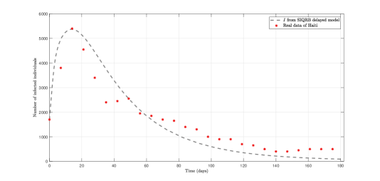
Figure 2. Numerical solution $I$ through the SIQRB delayed model for values of Table 1 with $\tau=2.0$, $\delta=0.020$, $\beta=0.70$ and $\alpha_{1}=0.0120$ (dashed grey line) versus real data of Haiti (red stars).

The best fitted values found were: $\tau=2.0$, $\delta=0.020$, $\beta=0.70$ and $\alpha_{1}=0.0120$ (see Figure 2). Note that all the other considered parameter values, with respect to the SIQRB delayed model, are presented in Table 1. All the numerical computations were carried out in Matlab with the help of its routines for the integration of model (1).

Table 1. Parameter values and initial conditions for the time-delayed SIQRB control model (9).

Parameter	Description	Value	Reference
$\Lambda$	Recruitment rate	$24.4N(0)/365\ 000$ (day-1)	[47]
$\mu$	Natural death rate	2.2493$\times 10^{-5}$ (day-1)	[48]
$\beta$	Ingestion rate	0.7 (day-1)	Best fitted
$\kappa$	Half saturation constant	$10^{6}$ (cell/ml)	[49]
$\omega$	Immunity waning rate	0.4/365 (day-1)	[7]
$\delta$	Quarantine rate	0.02 (day-1)	Best fitted
$\varepsilon$	Recovery rate	0.2 (day-1)	[6]
$\alpha_{1}$	Death rate (infective)	0.012 (day-1)	Best fitted
$\alpha_{2}$	Death rate (quarantined)	0.0001 (day-1)	[6]
$\eta$	Shedding rate (infective)	10 (cell/ml day-1 person-1)	[11]
$d$	Bacteria death rate	0.33 (day-1)	[11]
$\tau$	Time delay associated to the state	2 (days)	Best fitted in agreement with [5]
$S(0)$	Susceptible individuals at $t=0$	5750 (person)	Assumed
$I(0)$	Infective individuals at $t=0$	1700 (person)	[32]
$Q(0)$	Quarantined individuals at $t=0$	0 (person)	Assumed
$R(0)$	Recovered individuals at $t=0$	0 (person)	Assumed
$B(0)$	Bacterial concentration at $t=0$	$275\times 10^{3}$ (cell/ml)	Assumed
$T$	Final time	182 (days)	[32]
$W_{u}$	Measure of the treatment cost	$1000$	Assumed
$u_{\max}$	Maximum value of the control	$4$	Assumed

5. Optimal control problem for the time-delayed SIQRB model

In the current section, we begin by formulating an optimal control problem related with the delayed SIQRB model (1) and then we apply the Pontryagin Minimum Principle. We end Section 5 with the study of several numerical solutions of the proposed optimal control problem varying the weights $W_{I}$ and $W_{B}$ of the cost functional associated with classes $I$ and $B$, respectively. These studies are done with the purpose to obtain control strategies that could have stopped the spread of the outbreak in Haiti considered in Section 4. In order to simplify the notation, we consider throughout the current section that the state variable is

$$X=(x_{1},x_{2},x_{3},x_{4},x_{5})=(S,I,Q,R,B).$$

5.1. Formulation of the optimal control problem

We propose a time-delayed optimal control problem associated with model (1). The set of differential equations of such optimal control problem is obtained by adding to model (1) a control function $u(\cdot)$ taking values in $\left[1,u_{\max}\right]$, which accelerates the movement from class $I$ to $Q$. In practice, by applying such control measure, infected individuals can be put under quarantine faster. If $u\equiv 1$, then all infective individuals are quarantined at the end of $\frac{1}{\delta}=\frac{1}{0.02}=50$ days. On the other hand, if $u\equiv u_{\max}$, then all infective people are put under quarantine at the end of $\frac{1}{\delta u_{\max}}<50$ days. The model with control is given by the following system of non-linear and delayed ordinary differential equations:

$$\begin{cases}\begin{split}\dot{S}(t)&=\Lambda-\displaystyle\frac{\beta B(t)}{\kappa+B(t)}S(t)+\omega R(t)-\mu S(t),\\[4.26773pt] \dot{I}(t)&=\displaystyle\frac{\beta B(t-\tau)}{\kappa+B(t-\tau)}S(t-\tau)-(\delta u(t)+\alpha_{1}+\mu)I(t),\\[4.26773pt] \dot{Q}(t)&=\delta u(t)I(t)-(\varepsilon+\alpha_{2}+\mu)Q(t),\\[4.26773pt] \dot{R}(t)&=\varepsilon Q(t)-(\omega+\mu)R(t),\\[4.26773pt] \dot{B}(t)&=\eta I(t)-dB(t),\\[2.84544pt] \end{split}\end{cases}$$ (9)

with initial conditions given by

$$S(t)=S_{0}\geq 0\,,\quad I(t)=I_{0}\geq 0\,,\quad Q(t)=Q_{0}\geq 0\,,\quad R(t)=R_{0}\geq 0\,\quad\text{and}\quad B(t)=B_{0}\geq 0\,$$ (10)

for all $t\in[-\tau,0]$. Our aim is to minimize the number of infective individuals and the bacterial concentration, as well as the cost of interventions associated with the control treatment through quarantine. Thus, we consider the following objective functional:

$$J\big{(}X(\cdot),u(\cdot)\big{)}=\int_{0}^{T}\big{(}W_{I}I(t)+W_{B}B(t)+W_{u}u(t)\big{)}dt\,,$$ (11)

where $T>0$ is the final time, $W_{I}>0$ and $W_{B}>0$ are the weights associated with infected individuals and bacterial concentration in the environment, respectively, and constant $W_{u}>0$ is a measure of the cost of interventions associated with the control $u$. It is important to emphasize that it is more appropriate to use a linear control integrand in the biomedical framework, as we do in (11), since the cost is directly proportional to the dosage control. Moreover, in real life, it is easier to apply a linear control measure than a quadratic one (see [45, 46]). The set $\mathcal{X}$ of admissible trajectories is given by

$$\mathcal{X}=\big{\{}X(\cdot)\in W^{1,1}\big{(}[0,T];\mathbb{R}^{5}\big{)}\,|\,\eqref{ModeloColeraControlo}\text{ and }\eqref{eq:init:cond_delay_OC}\text{ are satisfied}\big{\}}$$

and the admissible control set $\mathcal{U}$ is given by

$$\mathcal{U}=\big{\{}u(\cdot)\in L^{1}\big{(}[0,T];\mathbb{R}\big{)}\,|\,1\leq u(t)\leq u_{\max},\,\forall\,t\in[0,T]\,\big{\}}.$$

Recall that $W^{1,1}$ and $L^{1}$ are, respectively, the class of absolutely continuous functions and the space of Lebesgue integrable functions.

The optimal control problem consists of determining the vector function

$$X^{\diamond}(\cdot)=\big{(}S^{\diamond}(\cdot),I^{\diamond}(\cdot),Q^{\diamond}(\cdot),R^{\diamond}(\cdot),B^{\diamond}(\cdot)\big{)}\in\mathcal{X}$$

associated with an admissible control $u^{\diamond}(\cdot)\in\mathcal{U}$ on the time interval $[0,T]$, minimizing the cost functional (11), i.e.,

$$J\big{(}X^{\diamond}(\cdot),u^{\diamond}(\cdot)\big{)}=\min_{(X(\cdot),u(\cdot))\in\mathcal{X}\times\mathcal{U}}J\big{(}X(\cdot),u(\cdot)\big{)}.$$ (12)

5.2. Necessary optimality conditions: the Pontryagin Minimum Principle

The necessary optimality conditions for an optimal solution of (12) are given by the Pontryagin Minimum Principle for time-delayed optimal control problems [33, 34]. Let us denote the delayed state variables in the following way:

1. $S(t-\tau)=x_{1}(t-\tau)=y_{1}(t)$;

2. $B(t-\tau)=x_{5}(t-\tau)=y_{5}(t)$.

The Hamiltonian function associated with our optimal control problem is given by

$$\begin{split}H(X,y_{1},y_{5},u,\lambda)&=\ W_{I}x_{2}+W_{B}x_{5}+W_{u}u+\lambda_{1}\left(\Lambda-\displaystyle\frac{\beta x_{1}x_{5}}{\kappa+x_{5}}+\omega x_{4}-\mu x_{1}\right)\\ &\quad+\lambda_{2}\left(\displaystyle\frac{\beta y_{1}y_{5}}{\kappa+y_{5}}-(\delta u+\alpha_{1}+\mu)x_{2}\right)+\lambda_{3}\Big{(}\delta ux_{2}-(\varepsilon+\alpha_{2}+\mu)x_{3}\Big{)}\\ &\quad+\lambda_{4}\Big{(}\varepsilon x_{3}-(\omega+\mu)x_{4}\Big{)}+\lambda_{5}(\eta x_{2}-dx_{5}).\end{split}$$ (13)

Let the pair $\big{(}X^{\diamond}(\cdot),u^{\diamond}(\cdot)\big{)}\in\mathcal{X}\times\mathcal{U}$ be an optimal solution of (12). Then, in agreement with [33, 34], there is an adjoint function $\lambda^{\diamond}(\cdot)=\big{(}\lambda_{1}^{\diamond}(\cdot),\lambda_{2}^{\diamond}(\cdot),\lambda_{3}^{\diamond}(\cdot),\lambda_{4}^{\diamond}(\cdot),\lambda_{5}^{\diamond}(\cdot)\big{)}\in W^{1,1}\big{(}[0,T];\mathbb{R}^{5}\big{)}$ such that the following conditions hold a.e. in $t\in[0,T]$:

1. the differential adjoint equations:

   $$\begin{cases}\begin{split}\dot{\lambda_{1}^{\diamond}}(t)&=-\frac{\partial H}{\partial x_{1}}[t]-\frac{\partial H}{\partial y_{1}}[t+\tau]\chi_{[0,T-\tau]}(t)\\ &=\frac{\beta x_{5}^{\diamond}(t)}{k+x_{5}^{\diamond}(t)}\Big{(}\lambda_{1}^{\diamond}(t)-\lambda_{2}^{\diamond}(t+\tau)\chi_{[0,T-\tau]}(t)\Big{)}+\mu\lambda_{1}^{\diamond}(t),\\[5.69046pt] \dot{\lambda_{2}^{\diamond}}(t)&=-\frac{\partial H}{\partial x_{2}}[t]=-W_{I}+{\lambda_{2}^{\diamond}(t)}\Big{(}\delta u^{\diamond}(t)+\alpha_{1}+\mu\Big{)}-\delta\lambda_{3}^{\diamond}(t)u^{\diamond}(t)-\eta\lambda_{5}^{\diamond}(t),\\[5.69046pt] \dot{\lambda_{3}^{\diamond}}(t)&=-\frac{\partial H}{\partial x_{3}}[t]=\Big{(}\varepsilon+\alpha_{2}+\mu\Big{)}\lambda_{3}^{\diamond}(t)-\varepsilon\lambda_{4}^{\diamond}(t),\\[5.69046pt] \dot{\lambda_{4}^{\diamond}}(t)&=-\frac{\partial H}{\partial x_{4}}[t]=-\omega\lambda_{1}^{\diamond}(t)+\Big{(}\omega+\mu\Big{)}\lambda_{4}^{\diamond}(t),\\[5.69046pt] \dot{\lambda_{5}^{\diamond}}(t)&=-\frac{\partial H}{\partial x_{5}}[t]-\frac{\partial H}{\partial y_{5}}[t+\tau]\chi_{[0,T-\tau]}(t)\\ &=-W_{B}+\frac{\beta kx_{1}^{\diamond}(t)}{\big{(}k+x_{5}^{\diamond}(t)\big{)}^{2}}\Big{(}\lambda_{1}^{\diamond}(t)-\lambda_{2}^{\diamond}(t+\tau)\chi_{[0,T-\tau]}(t)\Big{)}+d\lambda_{5}^{\diamond}(t);\\[2.84544pt] \end{split}\end{cases}$$ (14)

2. the transversality conditions

   $$\lambda^{\diamond}(T)=0,$$

   in view of the free terminal state $X(T)$;

3. the minimality condition:

   $$H\big{(}X^{\diamond}(t),y_{1}^{\diamond}(t),y_{5}^{\diamond}(t),u^{\diamond}(t),\lambda^{\diamond}(t)\big{)}=\min_{u\in\mathcal{U}_{0}}H\big{(}X^{\diamond}(t),y_{1}^{\diamond}(t),y_{5}^{\diamond}(t),u,\lambda^{\diamond}(t)\big{)},$$ (15)

   where

   $$\mathcal{U}_{0}=\big{\{}u\in\mathbb{R}\,|\,1\leq u\leq u_{\max}\big{\}}.$$

Note that the Hamiltonian (13) is linear in the control variable. Hence, the minimizing control is determined by the sign of the switching function

$$\phi(t)=\frac{\partial H}{\partial u}[t]=W_{u}+\delta x_{2}^{\diamond}(t)\Big{(}\lambda_{3}^{\diamond}(t)-\lambda_{2}^{\diamond}(t)\Big{)}$$ (16)

as

$$u^{\diamond}(t)=\begin{cases}\begin{split}&u_{\max},\ &&\text{if}\quad\phi(t)<0;\\ &1,\ &&\text{if}\quad\phi(t)>0;\\ &\text{singular},\ &&\text{if}\quad\phi(t)=0\ \forall t\in I_{s}\subset[0,T].\end{split}\end{cases}$$ (17)

If the switching function has only finitely many isolated zeros in an interval $I_{b}\subset[0,T]$, then the control $u^{\diamond}$ is called bang-bang on $I_{b}$. In case of a singular control, where $\phi(t)=0$ on $I_{s}\subset[0,T]$, the Pontryagin Minimum Principle does not directly provide values of the control. We shall not discuss the singular case here, since in our computations we never encountered singular controls.

When we write $H[t]$, we mean that the arguments of the Hamiltonian $H$ are applied in $t$ along the extremal, that is, $H[t]=H\big{(}X^{\diamond}(t),y_{1}^{\diamond}(t),y_{5}^{\diamond}(t),u^{\diamond}(t),\lambda^{\diamond}(t)\big{)}$.

5.3. Numerical solutions of the time-delayed SIQRB control model

With the purpose to obtain strategies that could have stopped the spread of the cholera outbreak in Haiti mentioned in Section 4, we consider here that control measures are taken. The absence of a control measure means that we are considering $u(t)=1$ for all time $t\in[0,T]$, i.e., all infected individuals are moved to quarantine at the end of 50 days. Our aim consists in obtaining a faster response with the minimum cost. To illustrate this, we are going to solve optimal control problem (12), considering several cases. For solving it, we apply the discretization methods developed in [33, 34]. The resulting large-scale non-linear programming problem (NLP) can be conveniently formulated using the Applied Modeling Programming Language – AMPL (see [39, 40]), which can be linked to several efficient optimization solvers. We use the Interior-Point optimization solver – IPOPT, developed by Wächter and Biegler [41], with tolerance $tol=10^{-8}$. As integration method, we implement Euler’s method with $T=182$ days and at least $12740$ grid points. In the following, we shall compare several solutions by considering three different combinations of weights $W_{I}$ and $W_{B}$:

1. Case 1: $W_{I}=W_{B}=1$;

2. Case 2: $W_{I}=10$ and $W_{B}=1$;

3. Case 3: $W_{I}=1$ and $W_{B}=10$.

For these computations, we use the other parameters values and the initial conditions of Table 1.

Case 1 ($\mathbf{W_{I}=W_{B}=1}$). The obtained cost functional value and initial values of the adjoint variables are, approximately, given by

$$J_{1}(X^{\diamond},u^{\diamond})\simeq 4.299001\times 10^{6}\quad\text{and}\quad\lambda^{\diamond}(0)\simeq(363.76,\ 379.71,\ 15.875,\ 17.704,\ 3.1978).$$

The control is bang-bang with one switch at $t=t^{s}$:

$$u^{\diamond}(t)=\begin{cases}\begin{split}&4,&&\mbox{if}\quad t\in\left[0,t^{s}\right],\\ &1,&&\mbox{if}\quad t\in\left]t^{s},T\right],\end{split}\end{cases}$$ (18)

where $t^{s}\simeq 87.843$ (see top left and right column of Figure 3). Note that the switching function satisfies the strict bang-bang property (see right column of Figure 4):

$$\begin{cases}\phi(t)<0\text{ for }t\in\left[0,t^{s}\right[,\\ \dot{\phi}(t^{s})>0,\\ \phi(t)>0\text{ for }t\in\left]t^{s},T\right].\end{cases}$$ (19)

Case 2 ($\mathbf{W_{I}=10}$ and $\mathbf{W_{B}=1}$). The obtained cost functional value and initial values of the adjoint variables are, approximately, given by

$$J(X^{\diamond},u^{\diamond})\simeq 5.166139\times 10^{6}\quad\text{and}\quad\lambda^{\diamond}(0)\simeq(465.69,\ 490.35,\ 18.875,\ 21.210,\ 3.2784).$$

The control has also the bang-bang structure (18) with $t^{s}\simeq 91.79$ (see left column of Figure 3) and the switching function also satisfies the strict bang-bang property, as in (19) (see right column of Figure 5).

Case 3 ($\mathbf{W_{I}=1}$ and $\mathbf{W_{B}=10}$). The obtained cost functional value and initial values of the adjoint variables are, approximately, given by

$$J(X^{\diamond},u^{\diamond})\simeq 3.7821542\times 10^{7}\quad\text{and}\quad\lambda^{\diamond}(0)\simeq(3450.2,\ 3734.6,\ 100.66,\ 117.78,\ 32.964).$$

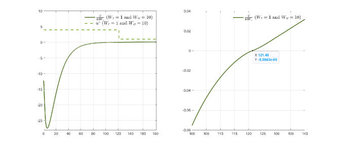
Figure 6. Extremal control $u^{\diamond}$, satisfying control law (17), and $\frac{\phi}{10W_{2}}$ (left column), as well as a zoom of $\frac{\phi}{10W_{u}}$ (right column), for problem (12) in Case 3, with the parameter values of Table 1.

Again, the control has the bang-bang structure (18) with $t^{s}\simeq 121.45$ (see top left and bottom right column of Figure 3) and the switching function satisfies the strict bang-bang property (see right column of Figure 6), as in (19).

Figures 3–6 summarize, in the three cases, our numerical findings associated with the extremal controls, while Figure 7 represents the corresponding extremal trajectories. The main message of Figures 4–6 is that the controls we have obtained numerically satisfy, always, the control law (17). Hence, the necessary conditions are satisfied and thus we have found the extremals. However, we remark that it does not suffice to check the strict bang-bang property to conclude that extremal controls are optimal. For time-delayed optimal control problems with bang-bang solutions, it remains an open question to prove a second order sufficient optimality condition.

With respect to all considered cases, we present in Figures 4, 5 and 6 function $\frac{\phi}{cW}$, where $c$ is a positive constant, instead of $\phi$, because the values obtained by $\phi$ are much bigger than those achieved by control $u^{\diamond}$. Thus, using function $\frac{\phi}{cW}$, it is possible to compare the signal of $\phi$ with the behaviour of the extremal control $u^{\diamond}$ in the same plot.

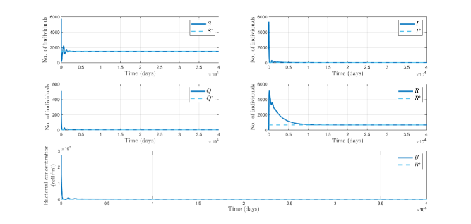
Figure 8. Asymptotic stability of the endemic equilibrium $(S^{*},I^{*},Q^{*},R^{*},B^{*})$ of model (1), using all the values of Table 1.

Figure 7 shows the comparison of the extremal state trajectories $S^{\diamond}$, $I^{\diamond}$, $Q^{\diamond}$, $R^{\diamond}$ and $B^{\diamond}$ for the optimal control problem (12), considering the parameter values of Table 1, for the three studied cases. Note that, although one can see that the obtained trajectories are very similar in all the cases, the controls corresponding to the three cases are very different, as well as the associated costs (see Figure 3) which implies different policies to control the outbreak. Furthermore, we also observed numerically that the endemic equilibrium (5) of the delayed model (1) is locally asymptotic stable, when we consider all the values of Table 1 (see Figure 8).

6. Conclusions

The paper is devoted to the formulation and analysis of a time-delayed mathematical model for cholera. We have improved our recent results by adding a time delay, which represents the time between the instant at which an individual becomes infected and the instant at which he begins to have symptoms of cholera infection by the bacterium Vibrio cholerae. The considered model is a SIQR (Susceptible–Infectious–Quarantined–Recovered) system, where an additional class $B$ is considered: a class of bacterial concentration in the dynamics of cholera. The host population is divided into four classes: susceptible, infectious with symptoms, quarantined, and recovered. An additional compartment reflects the bacterial concentration. The formulated model is analyzed, providing the non-negativity of the solutions for non-negative initial conditions, as well as the disease-free equilibrium, basic reproduction number, and endemic equilibrium. For positive time delays, the stability of the equilibrium points is also analyzed. Then, we consider the cholera outbreak that occurred in Haiti in 2010 and 2011. Finally, a SIQRB time-delayed optimal control problem, with linear cost functional, is formulated and analyzed numerically.

The delayed model is more realistic and describes better the reality, since the symptoms of cholera disease can appear from a few hours up to five days after infection. Usually, the symptoms appear in 2–3 days after infection (see [5]). We proved the positivity of the solutions of the delayed SIQRB model and analyzed the local asymptotic stability of the equilibrium points. Our analysis shows that the ingestion rate of the bacteria through contaminated sources $\beta$ has an important influence on the stability of the endemic equilibrium. We improved the numerical simulations done in [16] for the cholera outbreak in the Department of Artibonite – Haiti, from 1 November 2010 to 1 May 2011 [32], and showed that the delayed model fits better this cholera outbreak. A delayed optimal control problem was proposed and analyzed with a $L^{1}$ cost functional, where the objective is to minimize the number of infective individuals and the bacterial concentration, as well as the cost of interventions associated with the control treatment through quarantine. Necessary optimality conditions were applied to all considered cases of the optimal control problem. The delayed optimal control problems were solved numerically, applying the discretization methods developed in [33, 34]. Summarizing, the main contributions and novelties of our paper are: (i) the proposal of a more realistic cholera model with time delays; (ii) a local asymptotic stability analysis with respect to the proposed cholera model; (iii) the proposal, for the new model, of a more appropriate optimal control problem, in the biomedical framework, with linear cost measure, instead of a quadratic one as considered before in the literature; (iv) a numerical study of the proposed model and optimal control problem in order to translate cholera Haiti outbreak and to provide a control measure to stop the disease spread, respectively.

As future research directions, it remains to obtain (i) sufficient conditions for the local asymptotic stability of the endemic equilibrium, as well as the study of global stability, and (ii) second order sufficient optimality conditions for time-delayed optimal control problems with bang-bang solutions. Furthermore, as we have some parameters for which we only know an interval of values where they belong, it could be interesting to relate some of them under inequality constraints. Thus, we also point out, as future work, the study of parametric optimal control problems for cholera, by applying parameter sensitivity analysis.

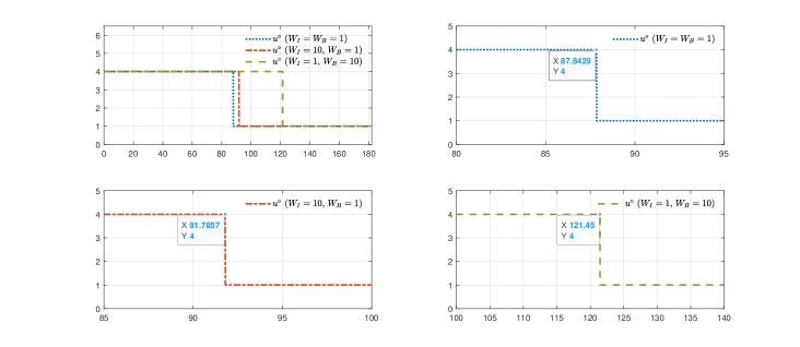
Figure 3. Extremal control $u^{\diamond}$ and zoom of it for Cases 1, 2 and 3 (dashed blue, dashed orange and dashed light green curves, respectively) associated with the optimal control problem (12), considering parameter values of Table 1.

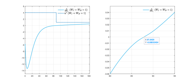
Figure 4. Extremal control $u^{\diamond}$, satisfying control law (17), and $\frac{\phi}{2W_{u}}$ (left column), as well as a zoom of $\frac{\phi}{2W_{u}}$ (right column), for problem (12) in Case 1, with the parameter values of Table 1.

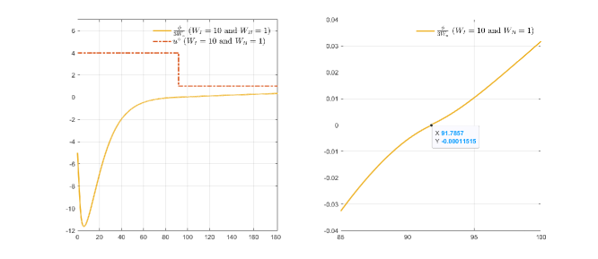
Figure 5. Extremal control $u^{\diamond}$, satisfying control law (17), and $\frac{\phi}{3W_{u}}$ (left column), as well as a zoom of $\frac{\phi}{3W_{u}}$ (right column), for problem (12) in Case 2, with the parameter values of Table 1.

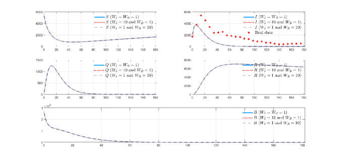
Figure 7. Extremal trajectories $S^{\diamond}$, $I^{\diamond}$, $Q^{\diamond}$, $R^{\diamond}$ and $B^{\diamond}$ of the optimal control problem (12), considering parameter values of Table 1, for Cases 1, 2 and 3 (solid light blue, dashed red, and dashed grey curves, respectively).

This research was supported by the Portuguese Foundation for Science and Technology (FCT) within projects UIDB/04106/2020 and UIDP/04106/2020 (CIDMA). Lemos-Paião was also supported by the Ph.D. fellowship PD/BD/114184/2016 and Silva by the FCT Researcher Program CEEC Individual 2018 with reference CEECIND/00564/2018. The authors are grateful to an Associate Editor and two anonymous Referees, who kindly reviewed an earlier version of the manuscript and provided several valuable suggestions and comments.

References

- [1] J. Cui, Z. Wu, X. Zhou, Mathematical analysis of a cholera model with vaccination, J. Appl. Math. (2014) Art. ID 324767, 16. http://dx.doi.org/10.1155/2014/324767
- [2] A. K. T. Kirschner, J. Schlesinger, A. H. Farnleitner, R. Hornek, B. Süß, B. Golda, A. Herzig, B. Reitner, Rapid growth of planktonic vibrio cholerae non-O1/non-O139 strains in a large alkaline lake in Austria: Dependence on temperature and dissolved organic carbon quality, Appl. Environ. Microbiol. 74 (7) (2008) 2004–2015. http://dx.doi.org/10.1128/AEM.01739-07
- [3] J. Reidl, K. E. Klose, Vibrio cholerae and cholera: out of the water and into the host, FEMS Microbiology Reviews 26 (2) (2002) 125–139. http://dx.doi.org/10.1111/j.1574-6976.2002.tb00605.x
- [4] Z. Shuai, J. H. Tien, P. van den Driessche, Cholera models with hyperinfectivity and temporary immunity, Bull. Math. Biol. 74 (10) (2012) 2423–2445. http://dx.doi.org/10.1007/s11538-012-9759-4
- [5] Centers for Disease Control and Prevention, Cholera – vibrio cholerae infection (2018), available from https://www.cdc.gov/cholera/general/index.html
- [6] A. Mwasa, J. M. Tchuenche, Mathematical analysis of a cholera model with public health interventions, Biosystems 105 (3) (2011) 190–200. http://dx.doi.org/10.1016/j.biosystems.2011.04.001
- [7] R. L. Miller Neilan, E. Schaefer, H. Gaff, K. R. Fister, S. Lenhart, Modeling optimal intervention strategies for cholera, Bull. Math. Biol. 72 (8) (2010) 2004–2018. http://dx.doi.org/10.1007/s11538-010-9521-8
- [8] M. O. Beryl, L. O. George, N. O. Fredrick, Mathematical analysis of a cholera transmission model incorporating media coverage, Int. J. Pure Appl. Math. 111 (2) (2016) 219–231. http://dx.doi.org/10.12732/ijpam.v111i2.8
- [9] G.-Q. Sun, J.-H. Xie, S.-H. Huang, Z. Jin, M.-T. Li, L. Liu, Transmission dynamics of cholera: mathematical modeling and control strategies, Commun. Nonlinear Sci. Numer. Simul. 45 (2017) 235–244. http://dx.doi.org/10.1016/j.cnsns.2016.10.007
- [10] V. Capasso, S. L. Paveri-Fontana, A mathematical model for the 1973 cholera epidemic in the European Mediterranean region, Rev. Epidemiol. Santé Publique 27 (2) (1979) 121–132.
- [11] F. Capone, V. De Cataldis, R. De Luca, Influence of diffusion on the stability of equilibria in a reaction-diffusion system modeling cholera dynamic, J. Math. Biol. 71 (5) (2015) 1107–1131. http://dx.doi.org/10.1007/s00285-014-0849-9
- [12] C. T. Codeço, Endemic and epidemic dynamics of cholera: the role of the aquatic reservoir, BMC Infect. Dis. 1 (1) (2001) 14 pp. http://dx.doi.org/10.1186/1471-2334-1-1
- [13] D. M. Hartley, J. G. Morris, Jr., D. L. Smith, Hyperinfectivity: A critical element in the ability of V. cholerae to cause epidemics?, PLOS Med. 3 (1) (2006) 63–69. http://dx.doi.org/10.1371/journal.pmed.0030007
- [14] S. D. Hove-Musekwa, F. Nyabadza, C. Chiyaka, P. Das, A. Tripathi, Z. Mukandavire, Modelling and analysis of the effects of malnutrition in the spread of cholera, Math. Comput. Modelling 53 (9-10) (2011) 1583–1595. http://dx.doi.org/10.1016/j.mcm.2010.11.060
- [15] R. I. Joh, H. Wang, H. Weiss, J. S. Weitz, Dynamics of indirectly transmitted infectious diseases with immunological threshold, Bull. Math. Biol. 71 (4) (2009) 845–862. http://dx.doi.org/10.1007/s11538-008-9384-4
- [16] A. P. Lemos-Paião, C. J. Silva, D. F. M. Torres, An epidemic model for cholera with optimal control treatment, J. Comput. Appl. Math. 318 (2017) 168–180. http://dx.doi.org/10.1016/j.cam.2016.11.002 arXiv:1611.02195
- [17] Z. Mukandavire, F. K. Mutasa, S. D. Hove-Musekwa, S. Dube, J. M. Tchuenche, Mathematical analysis of a cholera model with carriers and assessing the effects of treatment, Nova Science Publishers, Inc., 2008, pp. 1–37.
- [18] H. Nishiura, S. Tsuzuki, Y. Asai, Forecasting the size and peak of cholera epidemic in Yemen, 2017, Future Microbiol. 13 (4) (2018) 399–402. http://dx.doi.org/10.2217/fmb-2017-0244
- [19] H. Nishiura, S. Tsuzuki, B. Yuan, T. Yamaguchi, Y. Asai, Transmission dynamics of cholera in Yemen, 2017: a real time forecasting, Theor. Biol. Med. Model. 14 (1) (2017) 8 pp. http://dx.doi.org/10.1186/s12976-017-0061-x
- [20] M. Pascual, L. F. Chaves, B. Cash, X. Rodó, M. Yunus, Predicting endemic cholera: the role of climate variability and disease dynamics, Clim. Res. 36 (2) (2008) 131–140. http://dx.doi.org/10.3354/cr00730
- [21] J. Wang, C. Modnak, Modeling cholera dynamics with controls, Can. Appl. Math. Q. 19 (3) (2011) 255–273.
- [22] Q. Liu, D. Jiang, T. Hayat, A. Alsaedi, Dynamical behavior of a stochastic epidemic model for cholera, J. Franklin Inst. 356 (13) (2019) 7486–7514. https://doi.org/10.1016/j.jfranklin.2018.11.056
- [23] J. Wang, S. Liao, A generalized cholera model and epidemic-endemic analysis, J. Biol. Dyn. 6 (2) (2012) 568–589. http://dx.doi.org/10.1080/17513758.2012.658089
- [24] Z. Mukandavire, S. Liao, J. Wang, H. Gaff, D. L. Smith, J. G. Morris, Estimating the reproductive numbers for the 2008–2009 cholera outbreaks in Zimbabwe, Proc. Natl. Acad. Sci. 108 (21) (2011) 8767–8772. http://dx.doi.org/10.1073/pnas.1019712108
- [25] S. Edward, N. Nyerere, A mathematical model for the dynamics of cholera with control measures, Appl. Comput. Math. 4 (2) (2015) 53–63. http://dx.doi.org/10.11648/j.acm.20150402.14
- [26] B. Zhou, D. Jiang, Y. Dai, T. Hayat, Stationary distribution and density function expression for a stochastic SIQRS epidemic model with temporary immunity, Nonlinear Dyn. 105 (2021) 931–955. https://doi.org/10.1007/s11071-020-06151-y
- [27] J. Calatayud, J. Carlos Cortés, M. Jornet, Computing the density function of complex models with randomness by using polynomial expansions and the RVT technique. Application to the SIR epidemic model, Chaos Solit. Fractals 133 (2020) 109639. https://doi.org/10.1016/j.chaos.2020.109639
- [28] World Health Organization, Yemen: Weekly epidemiological bulletin W26 2018 (2018). Available at http://www.emro.who.int/images/stories/yemen/week_26.pdf?ua=1
- [29] D. He, X. Wang, D. Gao, J. Wang, Modeling the 2016–2017 Yemen cholera outbreak with the impact of limited medical resources, J. Theoret. Biol. 451 (2018) 80–85. http://dx.doi.org/10.1016/j.jtbi.2018.04.041
- [30] A. P. Lemos-Paião, C. J. Silva, D. F. M. Torres, A cholera mathematical model with vaccination and the biggest outbreak of world’s history, AIMS Mathematics 3 (4) (2018) 448–463. http://dx.doi.org/10.3934/Math.2018.4.448 arXiv:1810.05823
- [31] Asian Scientist, Math in a time of cholera (2017). https://www.asianscientist.com/2017/08/health/mathematical-model-yemen-cholera-outbreak
- [32] World Health Organization, Global Task Force on Cholera Control, Cholera country profile: Haiti (2011). http://www.who.int/cholera/countries/HaitiCountryProfileMay2011.pdf
- [33] L. Göllmann, D. Kern, H. Maurer, Optimal control problems with delays in state and control variables subject to mixed control-state constraints, Optimal Control Appl. Methods 30 (4) (2009) 341–365. http://dx.doi.org/10.1002/oca.843
- [34] L. Göllmann, H. Maurer, Theory and applications of optimal control problems with multiple time-delays, J. Ind. Manag. Optim. 10 (2) (2014) 413–441. http://dx.doi.org/10.3934/jimo.2014.10.413
- [35] X. Yang, L. Chen, J. Chen, Permanence and positive periodic solution for the single-species nonautonomous delay diffusive models, Comput. Math. Appl. 32 (4) (1996) 109–116. http://dx.doi.org/10.1016/0898-1221(96)00129-0
- [36] K. L. Cooke, P. van den Driessche, On zeroes of some transcendental equations, Funkcial. Ekvac. 29 (1) (1986) 77–90.
- [37] F. G. Boese, Stability with respect to the delay: on a paper of K. L. Cooke and P. van den Driessche. Comment on: “On zeroes of some transcendental equations” [Funkcial. Ekvac. 29 (1986), no. 1, 77–90; J. Math. Anal. Appl. 228 (2) (1998) 293–321. http://dx.doi.org/10.1006/jmaa.1998.6109
- [38] Y. Kuang, Delay differential equations with applications in population dynamics, Vol. 191 of Mathematics in Science and Engineering, Academic Press, Inc., Boston, MA, 1993.
- [39] R. Fourer, D. M. Gay, B. W. Kernighan, AMPL: A Modeling Language for Mathematical Programming, Scientific Press series, Thomson, Brooks, Cole, 2003.
- [40] D. M. Gay, The AMPL modeling language: an aid to formulating and solving optimization problems, in: Numerical analysis and optimization, Vol. 134 of Springer Proc. Math. Stat., Springer, Cham, 2015, pp. 95–116. http://dx.doi.org/10.1007/978-3-319-17689-5_5
- [41] A. Wächter, L. T. Biegler, On the implementation of an interior-point filter line-search algorithm for large-scale nonlinear programming, Math. Program. 106 (1, Ser. A) (2006) 25–57. http://dx.doi.org/10.1007/s10107-004-0559-y
- [42] H. Maurer, S. Pickenhain, Second-order sufficient conditions for control problems with mixed control-state constraints, J. Optim. Theory Appl. 86 (3) (1995) 649–667. http://dx.doi.org/10.1007/BF02192163
- [43] H. Schättler, U. Ledzewicz, H. Maurer, Sufficient conditions for strong local optimality in optimal control problems with -type objectives and control constraints, Discrete Contin. Dyn. Syst. Ser. B 19 (8) (2014) 2657–2679. http://dx.doi.org/10.3934/dcdsb.2014.19.2657
- [44] T. Guinn, Reduction of delayed optimal control problems to nondelayed problems, J. Optimization Theory Appl. 18 (3) (1976) 371–377. http://dx.doi.org/10.1007/BF00933818
- [45] U. Ledzewicz, H. Schättler, Controlling a model for bone marrow dynamics in cancer chemotherapy, Math. Biosci. Eng. 1 (1) (2004) 95–110. http://dx.doi.org/10.3934/mbe.2004.1.95
- [46] U. Ledzewicz, H. Schättler, On optimal singular controls for a general SIR-model with vaccination and treatment, Discrete Contin. Dyn. Syst. (2011) 981–990. http://dx.doi.org/10.3934/proc.2011.2011.981
- [47] Index Mundi, Demographics: Birth rate Haiti (2015). http://www.indexmundi.com/g/g.aspx?c=ha&v=25
- [48] Index Mundi, Demographics: Death rate Haiti (2015). http://www.indexmundi.com/g/g.aspx?c=ha&v=26
- [49] R. P. Sanches, C. P. Ferreira, R. A. Kraenkel, The role of immunity and seasonality in cholera epidemics, Bull. Math. Biol. 73 (12) (2011) 2916–2931. http://dx.doi.org/10.1007/s11538-011-9652-6