Topology-aware Generalization of Decentralized SGD

Abstract

This paper studies the algorithmic stability and generalizability of decentralized stochastic gradient descent (D-SGD). We prove that the consensus model learned by D-SGD is $\mathcal{O}{(N^{-1}\scalebox{0.75}[1.0]{$+$}m^{-1}\scalebox{0.75}[1.0]{$+$}\lambda^{2})}$-stable in expectation in the non-convex non-smooth setting, where $N$ is the total sample size, $m$ is the worker number, and $1\scalebox{0.75}[1.0]{$-$}\lambda$ is the spectral gap that measures the connectivity of the communication topology. These results then deliver an $\mathcal{O}{(N^{-(1\scalebox{0.75}[1.0]{$+$}\alpha)/2}\scalebox{0.75}[1.0]{$+$}m^{-(1+\alpha)/2}\scalebox{0.75}[1.0]{$+$}\lambda^{1+\alpha}\scalebox{0.75}[1.0]{$+$}\phi_{\mathcal{S}})}$ in-average generalization bound, which is non-vacuous even when $\lambda$ is closed to $1$, in contrast to vacuous as suggested by existing literature on the projected version of D-SGD. Our theory indicates that the generalizability of D-SGD is positively correlated with the spectral gap, and can explain why consensus control in initial training phase can ensure better generalization. Experiments of VGG-11 and ResNet-18 on CIFAR-10, CIFAR-100 and Tiny-ImageNet justify our theory. To our best knowledge, this is the first work on the topology-aware generalization of vanilla D-SGD. Code is available at https://github.com/Raiden-Zhu/Generalization-of-DSGD.

1 Introduction

Decentralized stochastic gradient descent (D-SGD) facilitates simultaneous model training on a massive number of workers without a central server (Lopes & Sayed, 2008; Nedic & Ozdaglar, 2009b). In D-SGD, every worker only communicates with the directly connected neighbors through “gossip communication” (Xiao & Boyd, 2004; Lian et al., 2017; Koloskova et al., 2020). The communication intensity is controlled by the communication topology. This decentralized nature eliminates the requirement for an expensive central server dedicated to heavy communication. Surprisingly, existing theoretical results demonstrate that the massive models on the edge converge to a unique steady model, the consensus model, even without the control of a central server (Lu et al., 2011; Shi et al., 2015; Lian et al., 2017). Compared with the centralized synchronized SGD (C-SGD) (Dean et al., 2012; Li et al., 2014), D-SGD can achieve the same asymptotic linear speedup in convergence rate (Lian et al., 2017). In this way, D-SGD provides a promising distributed machine learning paradigm with improved privacy (Nedic, 2020), scalability (Lian et al., 2017; Kairouz et al., 2021), and communication efficiency (Ying et al., 2021b).

To date, the theoretical research on D-SGD has mainly focused on its convergence (Nedic & Ozdaglar, 2009b; Lian et al., 2017; Koloskova et al., 2020; Alghunaim & Yuan, 2021), while the understanding on the generalizability (Mohri et al., 2018; He & Tao, 2020) of D-SGD is still premature. A large amount of empirical evidence have shown that D-SGD generalizes well on well-connected topologies (Assran et al., 2019a; Ying et al., 2021a). Meanwhile, empirical results by Assran et al. (2019b), Kong et al. (2021) and Ying et al. (2021a) demonstrate that for ring topologies, the validation accuracy of the consensus model learned by D-SGD decreases as the number of workers increases. Thus, a question is raised:

This paper answers this question. We prove a topology-aware generalization error bound for the consensus model learned by D-SGD, which characterizes the impact of the communication topology on the generalizability of D-SGD. Our contributions are summarized as follows:

• Stability and generalization bounds of D-SGD. This work proves the algorithmic stability (Bousquet & Elisseeff, 2002) and generalization bounds of vanilla D-SGD in the non-convex non-smooth setting. In Section 4, we present an $\mathcal{O}{(N^{-1}\scalebox{0.75}[1.0]{$+$}m^{-1}\scalebox{0.75}[1.0]{$+$}\lambda^{2})}$ distributed on-average stability (see Corollary 2), where $1-\lambda$ denotes the spectral gap of the network, a measure of the connectivity of the communication topology $\mathcal{G}$. These results would suffice to derive a $\mathcal{O}{(N^{-(1\scalebox{0.75}[1.0]{$+$}\alpha)/2}\scalebox{0.75}[1.0]{$+$}m^{-(1+\alpha)/2}\scalebox{0.75}[1.0]{$+$}\lambda^{1+\alpha}\scalebox{0.75}[1.0]{$+$}\phi_{\mathcal{S}})}$ generalization bound in expectation of D-SGD (see Theorem 4). Our error bounds are non-vacuous, even when the worker number is sufficiently large, or the communication graph is sufficiently sparse. The theory can be directly applied to explain why consensus distance control in the initial phase of training can ensure better generalization.

• Communication topology and generalization of D-SGD. Our theory shows that the generalizability of D-SGD has a positive relationship with the spectral gap $1-\lambda$ of the communication topology $\mathcal{G}$. Besides, we prove that the generalizability of D-SGD decreases when the worker number increases for the ring, grid, and exponential graphs. We conduct comprehensive experiments of VGG-11 (Simonyan & Zisserman, 2014) and ResNet-18 (He et al., 2016b) on CIFAR-10, CIFAR-100 (Krizhevsky et al., 2009) and Tiny-ImageNet (Le & Yang, 2015) to verify our theory.

To our best knowledge, this work offers the first investigation into the topology-aware generalizability of vanilla D-SGD. The closest work in the existing literature is by Sun et al. (2021), which derives $\mathcal{O}({N}^{-1}\scalebox{0.75}[1.0]{$+$}(1\scalebox{0.75}[1.0]{$-$}\lambda)^{-1})$ generalization bounds for projected D-SGD based on uniform stability (Bousquet & Elisseeff, 2002). They show that the decentralized nature hurts the stability, and thus undermines generalizability. Compared with the results by Sun et al. (2021), our work makes two contributions: (1) we analyze the vanilla D-SGD, which is capable of solving optimization problems on unbounded domains, rather than the projected D-SGD; and (2) our stability and generalization bounds are non-vacuous, even in the cases where the spectral gap $1\scalebox{0.75}[1.0]{$-$}\lambda$ is sufficiently close to $0$, which characterizes the cases where the worker number is sufficiently large or the communication graph is sufficiently sparse.

2 Related Work

The earliest work of classical decentralized optimization can be traced back to Tsitsiklis (1984), Tsitsiklis et al. (1986) and Nedic & Ozdaglar (2009a). D-SGD has been extended to various settings in deep learning, including time-varying topologies (Lu & Wu, 2020; Koloskova et al., 2020), asynchronous settings (Lian et al., 2018; Xu et al., 2021; Nadiradze et al., 2021), directed topologies (Assran et al., 2019a; Taheri et al., 2020), and data-heterogeneous scenarios (Tang et al., 2018; Vogels et al., 2021). It has been proved that the convergence of D-SGD heavily relies on the communication topology (Hambrick et al., 1996; Bianchi & Jakubowicz, 2012; Lian et al., 2017; Nedić et al., 2018; Assran et al., 2019b; Wang et al., 2019; Guo et al., 2020; Vogels et al., 2022), especially in the scenarios where the local data is heterogeneous across workers (Yuan et al., 2020; Koloskova et al., 2020; Bellet et al., 2021; Dai et al., 2022; Bars et al., 2022). However, the impact of the communication topology on the generalizability of D-SGD is still in its infancy.

Recently, inspiring work by Zhang et al. (2021) gives insights to how gossip communication in D-SGD promotes generalization in large batch settings. They prove that a self-adjusting noise exists in D-SGD, which may help D-SGD find flatter minima with better generalization. Another work by Richards et al. (2020) presents a generalization bound of the Adaptation-Then-Combination (ATC) version of D-SGD through algorithmic stability and Rademacher complexity (Mohri et al., 2018) in both smooth and non-smooth settings. However, their generalization bounds are invariant to the communication topology, which contradicts the experimental results (see Figure 3). In contrast, our generalization bounds are topology-aware and characterize the effects of decentralization on generalization.

3 Preliminaries

Supervised learning. Supposed $\mathcal{X}\subseteq\mathbb{R}^{d_{x}}$ and $\mathcal{Y}\subseteq\mathbb{R}$ are the input and output spaces, respectively. We denote the training set as $\mathcal{S}=\left\{z_{1},\ldots,z_{N}\right\}$, where $z_{\zeta}=\left(x_{\zeta},y_{\zeta}\right),\zeta=1,\dots,N$ are sampled independent and identically distributed (i.i.d.) from an unknown data distribution $\mathcal{D}$ defined on $\mathcal{Z}=\mathcal{X}\times\mathcal{Y}$.

The goal of supervised learning is to learn a predictor (hypothesis) $g(\cdot;\mathbf{w})$, parameterized by $\mathbf{w}=\mathbf{w}(z_{1},z_{2},\ldots,z_{N})\in\mathbb{R}^{d}$, to approximate the mapping between the input variable $x\in\mathcal{X}$ and the output variable $y\in\mathcal{Y}$, based on the training set $\mathcal{S}$. Let $c:\mathcal{Y}\times\mathcal{Y}\mapsto\mathbb{R}^{+}$ be a loss function that evaluates the prediction performance of the hypothesis $g$. The loss of a hypothesis $g$ with respect to (w.r.t.) the example $z_{\zeta}=(x_{\zeta},y_{\zeta})$ is denoted by $f(\mathbf{w};z_{\zeta})=c(g(x_{\zeta};\mathbf{w}),y_{\zeta})$, in order to measure the effectiveness of the learned model. Then, the empirical and population risks of $\mathbf{w}$ are defined as follows:

$$F_{\mathcal{S}}(\mathbf{w})=\frac{1}{N}\sum_{\zeta=1}^{N}f(\mathbf{w};z_{\zeta}),~{}~{}F(\mathbf{w})=\mathbb{E}_{z\sim D}[f(\mathbf{w};z)].$$

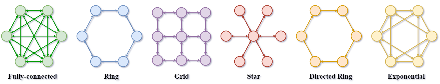
Figure 1: Illustration of some commonly-used communication topologies.

Distributed learning. Distributed learning jointly trains a learning model $\mathbf{w}$ on multiple workers (Shamir & Srebro, 2014). In this framework, the $k$-th worker $(k=1,\dots,m)$ can access $n_{k}$ independent and identically distributed (i.i.d.) training examples $\mathcal{S}_{k}=\{z_{k,1},\ldots,z_{k,n_{k}}\}$, drawn from the data distribution $\mathcal{D}$. If set $n_{k}=n$, the total sample size will be $N=nm$. In this case, the global empirical risk of $\mathbf{w}$ is

$$\hat{F}(\mathbf{w})=\frac{1}{m}\sum_{k=1}^{m}F_{\mathcal{S}_{k}}(\mathbf{w}),$$

where $F_{\mathcal{S}_{k}}(\mathbf{w})=\frac{1}{n}\sum_{\zeta=1}^{n}f({\mathbf{w}};z_{k,\zeta})$ denotes the local empirical risk on the $k$-th worker and $z_{k,\zeta}\in\mathcal{S}_{k}$ $(\zeta=1,\dots,n)$ is the local sample set.

Decentralized Stochastic Gradient Descent (D-SGD). The goal of D-SGD is to learn a consensus model $\overline{\mathbf{w}}=\frac{1}{m}\sum_{k=1}^{m}\mathbf{w}_{k}$, on $m$ workers, where $\mathbf{w}_{k}$ denotes the local model on the $k$-th worker. For any $k$, let $\mathbf{w}_{k}^{(t)}\in\mathbb{R}^{d}$ be the $d$-dimensional local model on the $k$-th worker in the $t$-th iteration, while $\mathbf{w}_{k}^{(1)}=0$ is the initial point. We denote $\mathbf{P}$ as a doubly stochastic gossip matrix that characterizes the underlying topology $\mathcal{G}$ (see Definition A.5 and Figure 1). The intensity of gossip communications is measured by the spectral gap (Seneta, 2006) of $\mathbf{P}$ (i.e., $1-\max\left\{\left|\lambda_{2}\right|,\left|\lambda_{n}\right|\right\}$, where $\lambda_{i}\ (i=2,\dots,m)$ denotes the $i$-th largest eigenvalue of $\mathbf{P}$ (see Definition A.6). The vanilla Adapt-While-Communicate (AWC) version of D-SGD without projecting operations updates the model on the $k$-th worker by

$$\mathbf{w}_{k}^{(t+1)}=\overbrace{\sum_{l=1}^{m}\mathbf{P}_{k,l}\mathbf{w}_{l}^{(t)}}^{\text{C}ommunication}-\overbrace{\eta_{t}\nabla f(\mathbf{w}_{k}^{(t)};z_{k,\zeta_{t}}^{(t)})}^{\text{C}omputation},$$ (1)

where $\{\eta_{t}\}$ is a sequence of positive learning rates, and $\nabla f(\mathbf{w}_{k}^{(t)};z_{k,\zeta_{t}}^{(t)})$ is the gradient of $f$ w.r.t. the first argument on the $k$-th worker, and $\zeta_{t}$ is i.i.d. variable drawn from the uniform distribution over $\{1,\ldots,n\}$ at the $t$-th iteration (Lian et al., 2017). In this paper, matrix $\mathbf{W}=[\mathbf{w}_{1},\cdots,\mathbf{w}_{m}]^{T}\in\mathbb{R}^{m\times d}$ stands for all local models across the network, while matrix $\nabla f(\mathbf{W};\mathbf{Z})=[\nabla f(\mathbf{w}_{1};z_{1}),\cdots,\nabla f(\mathbf{w}_{m};z_{m})]^{T}\in\mathbb{R}^{m\times d}$ stacks all local gradients w.r.t. the first argument. In this way, the matrix form of Eq. 1 is as follows:

$$\mathbf{W}^{(t+1)}=\mathbf{P}\mathbf{W}^{(t)}-\eta_{t}\nabla f(\mathbf{W}^{(t)};\mathbf{Z}^{(t)}_{\zeta_{t}}).$$

4 Topology-aware Generalization Bounds of D-SGD

This section proves stability and generalization bounds for D-SGD. We start with the definition of a new parameter-level stability for distributed settings. Then, the stability of D-SGD under a non-smooth condition is obtained (see Theorem 1 and Corollary 2). This implies a connection between stability and generalization in expectation (see Lemma 3), which suffices to prove the expected generalization bound of D-SGD, of order $\mathcal{O}{(N^{-(1\scalebox{0.75}[1.0]{$+$}\alpha)/2}\scalebox{0.75}[1.0]{$+$}m^{-(1+\alpha)/2}\scalebox{0.75}[1.0]{$+$}\lambda^{1+\alpha}\scalebox{0.75}[1.0]{$+$}\phi_{\mathcal{S}})}$.

4.1 Algorithmic Stability of D-SGD

Understanding generalization using algorithmic stability can be traced back to Bousquet & Elisseeff (2002) and Shalev-Shwartz et al. (2010), and has been applied to stochastic gradient methods (Hardt et al., 2016; Lei & Ying, 2020). For more details, please see Appendix B.

We define a new algorithmic stability of distributed optimization algorithms below, which better characterizes the on-average sensitivity of models across multiple workers.

Definition 1 (Distributed On-average Stability).

Let $\mathcal{S}_{k}=\{z_{k,1},\ldots,z_{k,n}\}$ denote the i.i.d. local samples on $k$-th worker drawn from the distribution $\mathcal{D}$. $\mathcal{S}=\cup_{k=1}^{m}\mathcal{S}_{k}=\{z_{1},\ldots,z_{N}\}$ then denotes the whole training set. $\mathcal{S}^{(i)}=\cup_{k=1}^{m}\mathcal{S}_{k}^{(i)}=\{z_{1},\ldots,\tilde{z}_{i},\ldots,z_{N}\}$ is formed by replacing the $i$-th element of $\mathcal{S}$ with a sample $\tilde{z}_{i}$ drawn from the distribution $\mathcal{D}$, where $\mathcal{S}_{k}^{(i)}$ denotes the new local training samples on $k$-th worker. We denote $\mathbf{w}_{k}$ and $\widetilde{\mathbf{w}}_{k}$ as the weight vectors on the $k$-th worker produced by the stochastic algorithm $A$ based on $\mathcal{S}$ and $\mathcal{S}^{(i)}$, respectively. $A$ is $\ell_{2}$ distributed on-average $\epsilon$-stable for all training data sets $\mathcal{S}$ and $\mathcal{S}^{(i)}$ if

$$\frac{1}{mN}\sum_{i=1}^{N}\sum_{k=1}^{m}\mathbb{E}_{\mathcal{S},\mathcal{S}^{(i)},A}\big{[}\|\mathbf{w}_{k}-\widetilde{\mathbf{w}}_{k}\|_{2}^{2}\big{]}\leq\epsilon^{2},$$

where $\mathbb{E}_{A}[\cdot]$ stands for the expectation w.r.t. the randomness of the algorithm $A$ (see more details in Appendix A).

We then prove that D-SGD is distributed on-average stable.

Theorem 1.

Let $\mathcal{S}_{k}$ and $\mathcal{S}^{(i)}_{k}$ $\ (k=1,\dots,m)$ be constructed in Definition 1. Let $\mathbf{w}^{(t)}_{k}$ and $\widetilde{\mathbf{w}}^{(t)}_{k}$ be the $t$-th iteration on the $k$-th worker produced by Eq. 1 based on $\mathcal{S}_{k}$ and $\mathcal{S}_{k}^{(i)}$ $(k=1,\dots,m)$ respectively, and $\{\eta_{t}\}$ be a non-increasing sequence of positive learning rates. We assume that for all $z\in\mathcal{Z}$, the function $\mathbf{w}\mapsto f(\mathbf{w};z)$ is non-negative with its gradient $\nabla f(\mathbf{w};z)$ being $(\alpha,L)$-Hölder continuous (see Assumption A.3). We further assume that the weight differences at the $t$-th iteration are multivariate normally distributed: $\mathbf{w}_{k}^{(t)}-\widetilde{\mathbf{w}}_{k}^{(t)}\stackrel{{\scriptstyle i.i.d.}}{{\sim}}\mathcal{N}(\mu_{t,k},\sigma_{t,k}^{2}I_{d})$ for all $k$ where $d$ denotes the dimension of weights, with unknown parameters $\mu_{t,k}$ and $\sigma_{t,k}$ satisfying some technical conditions (see Assumption A.4), and the worker number $m\geq\frac{1}{d\mu_{0}^{2}}$. Then we have the following:

$$\frac{1}{mN} \sum_{i=1}^{N}\sum_{k=1}^{m}\mathbb{E}_{\mathcal{S},\mathcal{S}^{(i)},A}\big{[}\big{\|}\mathbf{w}_{k}^{(t+1)}-\widetilde{\mathbf{w}}_{k}^{(t+1)}\big{\|}_{2}^{2}\big{]}$$

$$\leq \sum_{\tau=0}^{t}{C}^{t-\tau}\{\underbrace{\mathcal{O}{\big{(}(1-\frac{1}{m})\bm{\lambda^{2}}+\frac{1}{m}\big{)}}}_{\text{Error from decentralization}}$$

$$+\underbrace{\mathcal{O}{(\frac{{\eta_{\tau}}^{2}}{N}}\cdot\frac{1}{m}\sum_{k=1}^{m}\mathbb{E}_{\mathcal{S},A}\big{[}F_{\mathcal{S}}^{\frac{2\alpha}{1+\alpha}}(\mathbf{w}_{k}^{(\tau)})\big{]})}_{\mathcal{O}{(\frac{1}{N})}\text{ $\cdot$ Averaged empirical risk}}\},$$

where $C=2\eta_{0}L(1-\frac{1}{N})$ and $F_{\mathcal{S}}(\mathbf{w}_{k}^{(\tau)})$ is the local empirical risk of the $k$-th worker at iteration $\tau$.

Theorem 1 suggests that the distributed on-average stability of decentralized SGD is positively related to the spectral gap of the given topology and negatively related to the accumulation of the averaged empirical risk. See detailed proof in Subsection D.2.

We can obtain a simplified result with fixed learning rates.

Corollary 2 (Stability in Expectation with $\eta_{t}\equiv\eta$ ).

Suppose all the assumptions of Theorem 1 hold. With a fixed learning rate $\eta_{t}\equiv\eta\leq\frac{1}{2L}(1-\frac{2}{m})$, the distributed on-average stability of D-SGD can be bounded as

$$\frac{1}{mN} \sum_{i=1}^{N}\sum_{k=1}^{m}\mathbb{E}_{\mathcal{S},\mathcal{S}^{(i)},A}\big{[}\big{\|}\mathbf{w}_{k}^{(t+1)}-\widetilde{\mathbf{w}}_{k}^{(t+1)}\big{\|}_{2}^{2}\big{]}$$

$$\leq \frac{1}{1\scalebox{0.75}[1.0]{$-$}2\eta L(1\scalebox{0.75}[1.0]{$-$}\frac{1}{N})}\{\mathcal{O}{(\frac{{\epsilon_{\mathcal{S}}\eta}^{2}}{N})}+\underbrace{\mathcal{O}{\big{(}(1-\frac{1}{m})\bm{\lambda^{2}}+\frac{1}{m}\big{)}}}_{\text{Error from decentralization}}\},$$

where $\epsilon_{\mathcal{S}}$ denotes the upper bound of averaged empirical risk $\frac{1}{m}\sum_{k=1}^{m}\mathbb{E}_{\mathcal{S},A}\big{[}F_{\mathcal{S}}^{\frac{2\alpha}{1+\alpha}}(\mathbf{w}_{k}^{(t)})\big{]}$.

Corollary 2 shows that the distributed on-averge stability of D-SGD is of the order $\mathcal{O}{(N^{-1}\scalebox{0.75}[1.0]{$+$}m^{-1}\scalebox{0.75}[1.0]{$+$}\lambda^{2})}$. We defer the proof to Subsection D.2.

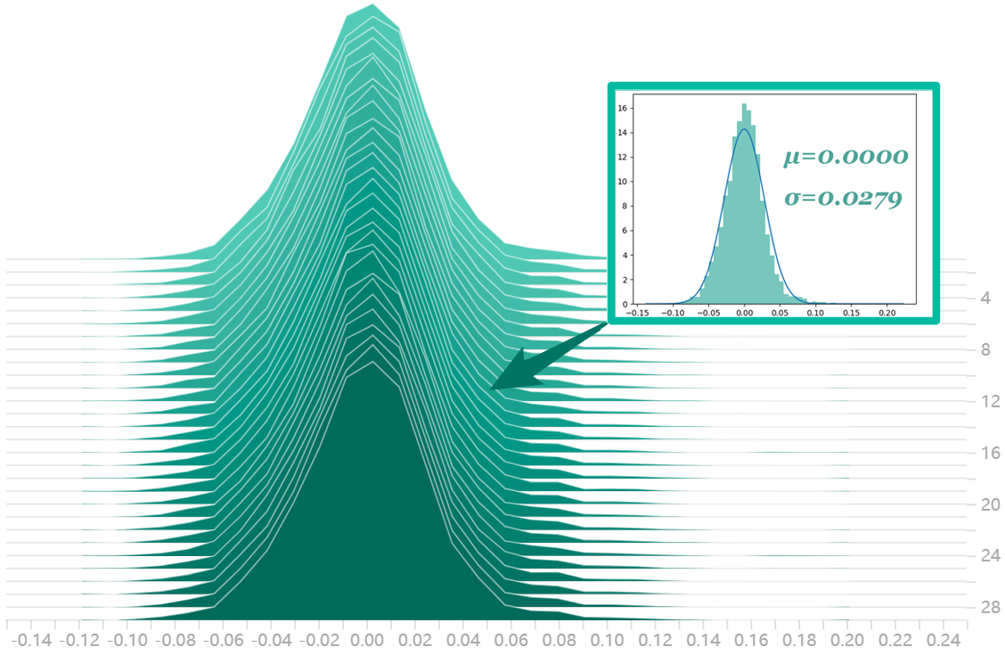
Figure 2: Histograms of the weight differences of the last layers of the ResNet-18 models (1024 dimensions $\times$ 10 classes=10240 parameters) trained by AWC D-SGD on $\mathcal{S}$ and $\mathcal{S}^{(i)}$ that differ by only one data point. Thirty ResNet-18 models are trained on data sampled from the MNIST dataset (LeCun et al., 1998), each model is trained with 16 workers for 3000 iterations.

Comparison with existing results.

Compared with Sun et al. (2021), we relax the restrictive bounded gradient and the smoothness assumptions. Instead, a much weaker Hölder condition (see Assumption A.3) is adopted. In addition, we make a mild assumption that the weight difference $\big{(}\mathbf{w}_{k}^{(t)}-\widetilde{\mathbf{w}}_{k}^{(t)}\big{)}$ is multivariate normally distributed (see Assumption A.4), which stems from our empirical observations: Figure 2 illustrates that the distribution of the weight differences in ResNet-18 models trained by D-SGD is close to a centered Gaussian. Intuitively, the assumption is based upon the fact that the weights of the consensus model are very insensitive to the change of a single data point.

We also compare the order of the derived bound with the existing literature. Hardt et al. (2016) proves that SGD is $\mathcal{O}{(\sum_{\tau=1}^{t-1}\eta_{\tau}/N)}$-stable in convex and smooth settings, which corresponds to the $\mathcal{O}{(\frac{1}{N})}$ term in Corollary 2. Under Hölder continuous condition, Lei & Ying (2020) proposes a parameter-level stability bound of SGD of the order $\mathcal{O}{(\frac{{\epsilon_{\mathcal{S}}\eta}^{2}}{N}\scalebox{0.75}[1.0]{$+$}\eta^{\frac{2}{1\scalebox{0.75}[1.0]{$-$}\alpha}})}$. In contrast, Corollary 2 shows that D-SGD suffers from additional terms $\mathcal{O}{\big{(}(1\scalebox{0.75}[1.0]{$-$}\frac{1}{m})\lambda^{2}\scalebox{0.75}[1.0]{$+$}\frac{1}{m}\big{)}}$, where the first term $\mathcal{O}{\big{(}(1\scalebox{0.75}[1.0]{$-$}\frac{1}{m})\lambda^{2}})$ can characterize the degree of disconnection of the underlying communication topology. Close work by Sun et al. (2021) proved that the stability of the projected variant of D-SGD is bounded by $\mathcal{O}\left(\frac{\eta tB^{2}}{N}\scalebox{0.75}[1.0]{$+$}\frac{\eta tB^{2}}{1\scalebox{0.75}[1.0]{$-$}\lambda}\right)$ in the convex smooth setting, where $B$ is the upper bound of the gradient norm. The term $\mathcal{O}{(\frac{\eta tB^{2}}{1\scalebox{0.75}[1.0]{$-$}\lambda})}$ brought by decentralization is of the order $\mathcal{O}{(m^{2}B^{2})}$ for ring topologies and $\mathcal{O}{(mB^{2})}$ for grids, respectively. Our error bound in Corollary 2 is tighter than their results, since

$$\frac{1}{1\scalebox{0.75}[1.0]{$-$}2\eta L(1\scalebox{0.75}[1.0]{$-$}\frac{1}{N})}\cdot\mathcal{O}{\big{(}(1-\frac{1}{m})\lambda^{2}+\frac{1}{m}\big{)}}\\ \leq\mathcal{O}{\big{(}m\big{)}}\ll\mathcal{O}{(mB^{2})}\leq\mathcal{O}{(m^{2}B^{2})}.$$

4.2 Generalization bounds of D-SGD

The following lemma bridges the gap between generalization and the newly proposed distributed on-average stability.

Lemma 3 (Generalization via Distributed On-average Stability).

Let $\mathcal{S}_{k}$ and $\mathcal{S}^{(i)}_{k}$ be constructed in Definition 1. If $\forall z$ the pre-specified function $f(\mathbf{w};z)$ is non-negative, with its gradient $\nabla f(\mathbf{w};z)$ being $(\alpha,L)$-Hölder continuous, and $\forall t$ $\mathbb{E}_{\mathcal{S},\mathcal{S}^{(i)},A}\|\frac{1}{m}\sum_{k=1}^{m}\mathbf{w}_{k}^{(t)}-\frac{1}{m}\sum_{k=1}^{m}\widetilde{\mathbf{w}}_{k}^{(t)}\|_{2}\leq 1$, then

$$\mathbb{E}_{\mathcal{S},A}\big{[}F(\overline{\mathbf{w}}^{(t)})\scalebox{0.75}[1.0]{$-$}F_{\mathcal{S}}(\overline{\mathbf{w}}^{(t)})\big{]}$$

$$\leq L_{\alpha,1}\big{\{}\frac{1}{mN}\sum_{k=1}^{m}\sum_{i=1}^{N}\mathbb{E}_{\mathcal{S},\mathcal{S}^{(i)},A}\big{[}\|\mathbf{w}_{k}^{(t)}\scalebox{0.8}{-}\widetilde{\mathbf{w}}_{k}^{(t)}\|_{2}^{2}\big{]}\big{\}}^{\frac{1\scalebox{0.6}{+}\alpha}{2}}\scalebox{0.8}{+}\phi_{\mathcal{S}},$$

where $\overline{\mathbf{w}}^{(t)}=\frac{1}{m}\sum_{k=1}^{m}\mathbf{w}_{k}^{(t)}$ represents the global averaged model, $L_{\alpha,1}=\frac{L}{1+\alpha}+\frac{1}{2}$ is a constant, and $\phi_{\mathcal{S}}=\mathbb{E}_{\mathcal{S},A}\big{[}\frac{1}{2N}\sum_{i=1}^{N}\|\nabla f(\overline{\mathbf{w}}^{(t)};z_{i})\|^{2}_{2}\big{]}$ denotes the empirical gradient norm.

We give the proof in Subsection D.3.

Lemma 3 suggests that if the consensus model learned by the distributed SGD $A$ is $\epsilon$-stable in the sense of Definition 1, the generalization error of the consensus model is bounded by $(\frac{L}{1\scalebox{0.6}{+}\alpha}\scalebox{0.8}{+}\frac{1}{2})\epsilon^{\frac{1\scalebox{0.8}{+}\alpha}{2}}\scalebox{0.8}{+}\phi_{\mathcal{S}}$. The last term $\phi_{\mathcal{S}}$ is very small for over-parameterized models near local or global minima (Vaswani et al., 2019). Lemma 3 improves Theorem 2 (c) of Lei & Ying (2020) by removing the $\mathcal{O}{(\mathbb{E}_{S,A}\big{[}F^{\frac{2\alpha}{1+\alpha}}(A(S))\big{]})}$ term, where $\mathbb{E}_{S,A}\big{[}F(A(S))\big{]}$ denotes the population risk of the learned model $A(\mathcal{S})$ (see Subsection D.3). This improvement is significant, because $\mathbb{E}_{S,A}\big{[}F(A(S))\big{]}$ usually does not converge to zero in practice.

We now prove the generalization bound of D-SGD based on Theorem 1 and Lemma 3.

Theorem 4 (Generalization Bound in Expectation with $\eta_{t}\equiv\eta$).

Let all the assumptions of Theorem 1 hold. With a fixed step sizes of $\eta_{t}\equiv\eta\leq 2L(1\scalebox{0.75}[1.0]{$-$}\frac{2}{m})$, the generalization error of the consensus model learned by D-SGD can be controlled as

$$\mathbb{E}_{\mathcal{S},A}\big{[}F(\overline{\mathbf{w}}^{(t)})\scalebox{0.75}[1.0]{$-$}F_{\mathcal{S}}(\overline{\mathbf{w}}^{(t)})\big{]}$$

$$\leq L_{\alpha,2}\{\mathcal{O}{((\frac{\epsilon_{\mathcal{S}}}{N})^{\frac{1\scalebox{0.6}{+}\alpha}{2}}\scalebox{0.75}[1.0]{$+$}\underbrace{{((1\scalebox{0.75}[1.0]{$-$}\frac{1}{m})\bm{\lambda^{2}}\scalebox{0.8}{+}\frac{1}{m})}^{\frac{1\scalebox{0.6}{+}\alpha}{2}}}_{{\text{Error from decentralization}}})}\}\scalebox{0.8}{+}\phi_{\mathcal{S}},$$

where $\overline{\mathbf{w}}^{(t)}=\frac{1}{m}\sum_{k=1}^{m}\mathbf{w}_{k}^{(t)}$ represents the global averaged model, $L_{\alpha,2}=(\frac{L}{1+\alpha}\scalebox{0.75}[1.0]{$+$}\frac{1}{2})/{[1\scalebox{0.75}[1.0]{$-$}2\eta L(1\scalebox{0.75}[1.0]{$-$}\frac{1}{n})]}^{\frac{1+\alpha}{2}}$ is a constant, $\phi_{\mathcal{S}}=\mathbb{E}_{\mathcal{S},A}\big{[}\frac{1}{2N}\sum_{i=1}^{N}\|\nabla f(\overline{\mathbf{w}}^{(t)};z_{i})\|^{2}_{2}\big{]}$ denotes the empirical gradient norm, and $\epsilon_{\mathcal{S}}$ is the upper bounder of $\frac{1}{m}\sum_{k=1}^{m}\mathbb{E}_{\mathcal{S},A}\big{[}F_{\mathcal{S}}^{\frac{2\alpha}{1+\alpha}}(\mathbf{w}_{k}^{(t)})\big{]}$.

The order of the generalization bound in Theorem 4 is $\mathcal{O}{(N^{-(1\scalebox{0.75}[1.0]{$+$}\alpha)/2}\scalebox{0.75}[1.0]{$+$}m^{-(1+\alpha)/2}\scalebox{0.75}[1.0]{$+$}\lambda^{1+\alpha}\scalebox{0.75}[1.0]{$+$}\phi_{\mathcal{S}})}$ and becomes $\mathcal{O}{(N^{-1}\scalebox{0.75}[1.0]{$+$}m^{-1}\scalebox{0.75}[1.0]{$+$}\lambda^{2}\scalebox{0.75}[1.0]{$+$}\phi_{\mathcal{S}})}$ in the smooth settings where $\alpha=1$. The proof is provided in Subsection D.3.

Remark 1.

Corollary 2 and Theorem 4 indicate that the stability and generalization of D-SGD are positively related to the spectral gap $1-\lambda$. The intuition of the results is that D-SGD with a denser connection topology (i.e., larger $\lambda$) can aggregate more information from its neighbors, thus “indirectly” accessing more data at each iteration, leading to better generalization.

4.3 Practical Implications

Our theory delivers significant practical implications.

Communication topology and generalization. The intensity of communication is controlled by the spectral gap $1-\lambda$ of the underlying communication topologies (see Table 1). Detailed analyses of the spectral gaps of some commonly-used topologies can be found in Proposition 5 of Nedić et al. (2018) and Ying et al. (2021a). Substituting the spectral gap of different topologies in Table 1 into Theorem 4, we can conclude that the generalization error of different topologies can be ranked as follows: fully-connected $<$ exponential $<$ grid $<$ ring, since

$$0<1-\mathcal{O}{((\log_{2}(m))^{-1})}\\ <1-\mathcal{O}{((m\log_{2}(m))^{-1})}<1-\mathcal{O}{(m^{-2})}.$$

Table 1: Spectral gap of gossip matrices with different topology.

Graph topoloy	Spectral gap $1-\lambda$
Disconnected	0
Ring	$\mathcal{O}{(1/m^{2})}$
Grid	$\mathcal{O}{(1/(m\log_{2}(m)))}$
Exponential	$\mathcal{O}{({1}/{\log_{2}(m))}}$
Fully-connected	1

On the one hand, our theory provides theoretical evidence that D-SGD generalizes better on well-connected topologies (i.e., topologies with larger spectral gap). On the other hand, we prove that for a specific topology, the worker number impacts the generalization of D-SGD through affecting the spectral gap of the topology.

Consensus distance control. Recently, a line of studies have been devoted to understanding the connection between optimization and generalization through studying the effect of early phase training (Keskar et al., 2017; Achille et al., 2018; Frankle et al., 2020). In the decentralized settings, Kong et al. (2021) claims that there exists a “critical consensus distance” in the initial training phase—consensus distance (i.e., $\frac{1}{m}\sum_{i=1}^{m}\|\mathbf{w}_{k}^{(t)}-\frac{1}{m}\sum_{k=1}^{m}\mathbf{w}_{k}^{(t)}\|^{2}_{F}$) below the critical threshold ensures good generalization. However, the reason why consensus distance control can promote generalization remains an open problem. Fortunately, the following theorem can explain this phenomenon by connecting the consensus distance notion in Kong et al. (2021) with the algorithmic stability and the generalizability of D-SGD.

Corollary 5.

Let all the assumptions of Theorem 1 plus Assumption A.1 and Assumption A.2 hold. Suppose that the consensus distance satisfies $\Gamma^{2}\leq\frac{1}{m}\sum_{k=1}^{m}\|\mathbf{w}_{k}^{(\tau)}-{\overline{\mathbf{w}}^{(\tau)}}\|_{2}^{2}\leq K^{2}$ for $\tau\leq t_{\Gamma}$, and is controlled below $\Gamma^{2}$ for $\tau>t_{\Gamma}$. We can conclude that the distributed on-average stability bound of D-SGD increases monotonically with $t_{\Gamma}$, if the total number of iterations $t\geq\frac{-C}{2\ln{C}}$.

We give the proof in Subsection D.4.

Corollary 5 provides theoretical evidence for the following empirical findings: (1) consensus control is beneficial for the algorithmic stability and thus for the generalizability of D-SGD; and (2) it is more effective to control the consensus distance at the initial stage of training than at the end of training.

5 Empirical Results

This section empirically validates our theoretical results. We first introduce the experimental setup and then study how the communication topology and the worker number affect the generalization of D-SGD. The code is available at https://github.com/Raiden-Zhu/Generalization-of-DSGD.

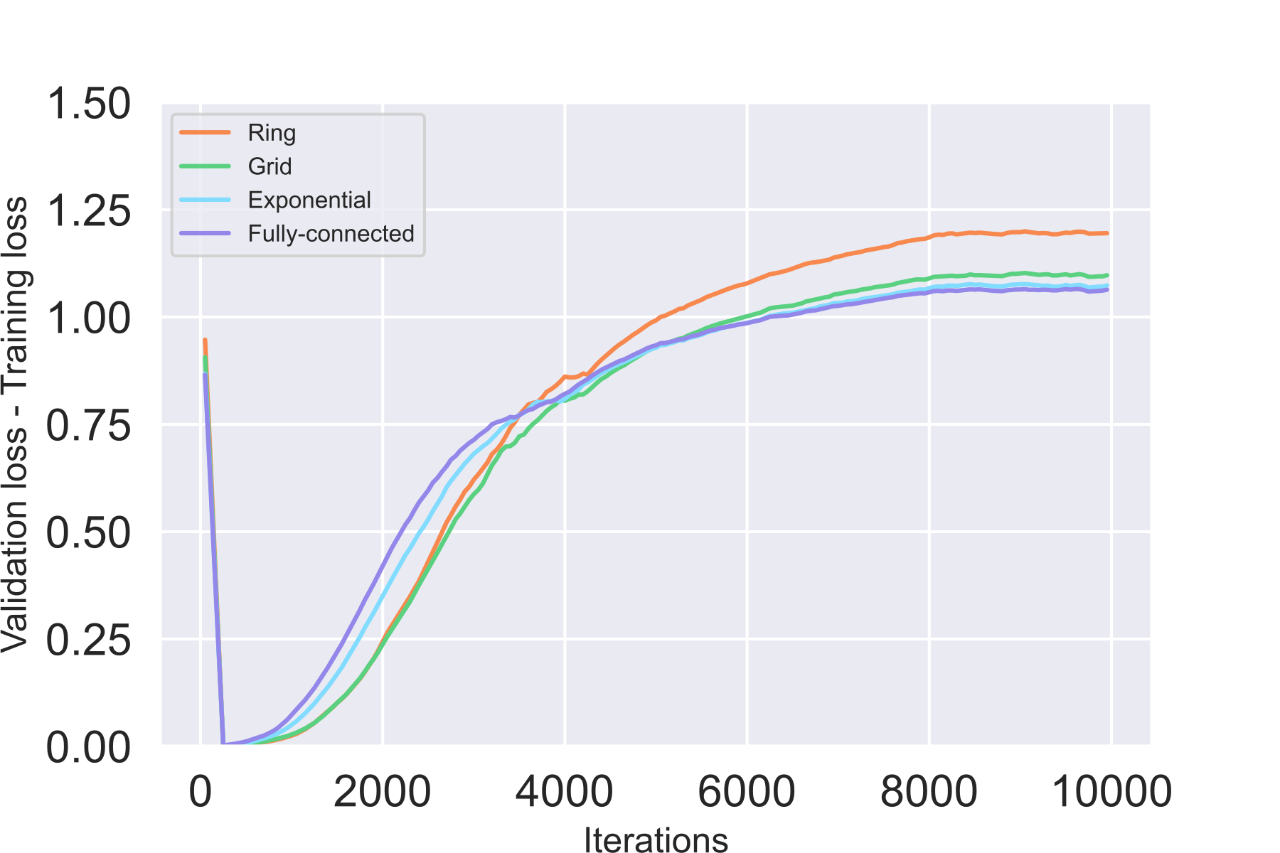
((a)) VGG-11 on CIFAR-10, 32 workers

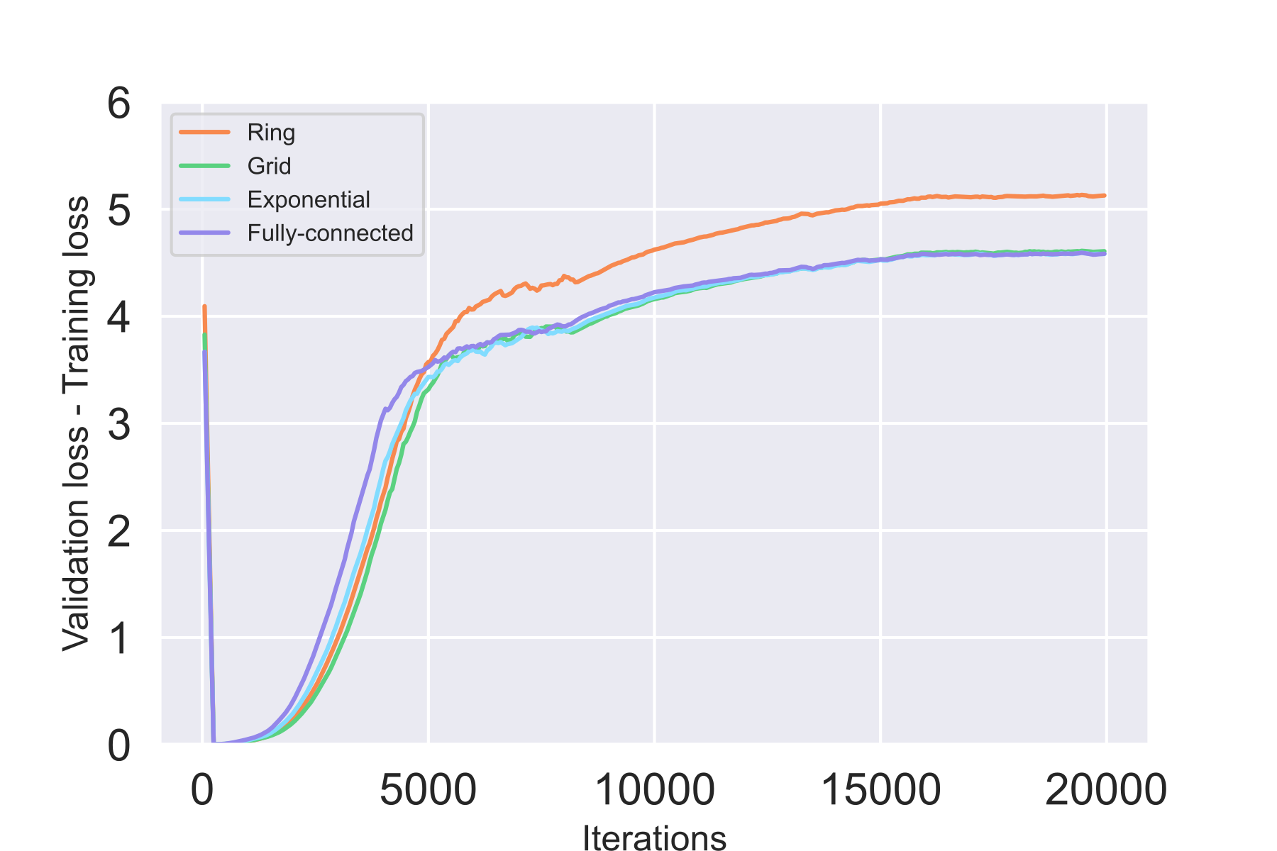
((b)) VGG-11 on CIFAR-100, 32 workers

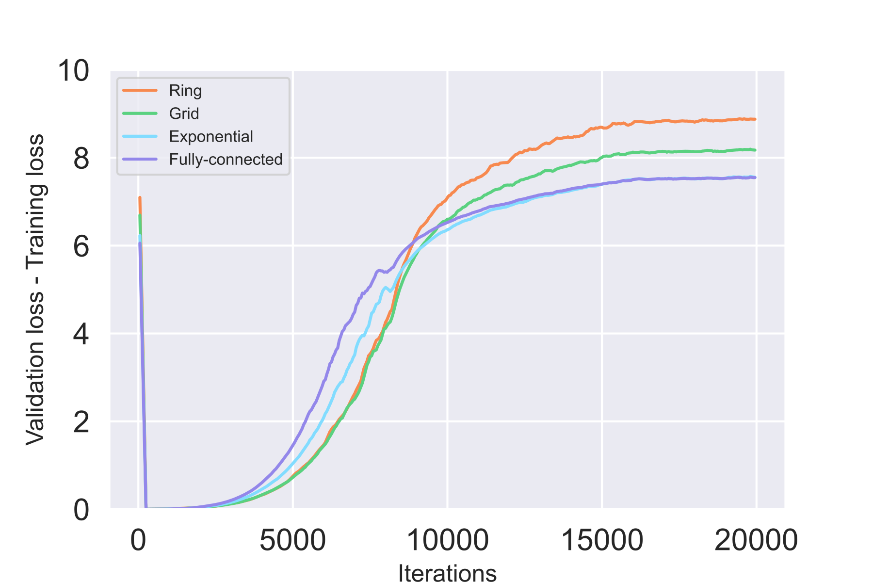
((c)) VGG-11 on Tiny ImageNet, 32 workers

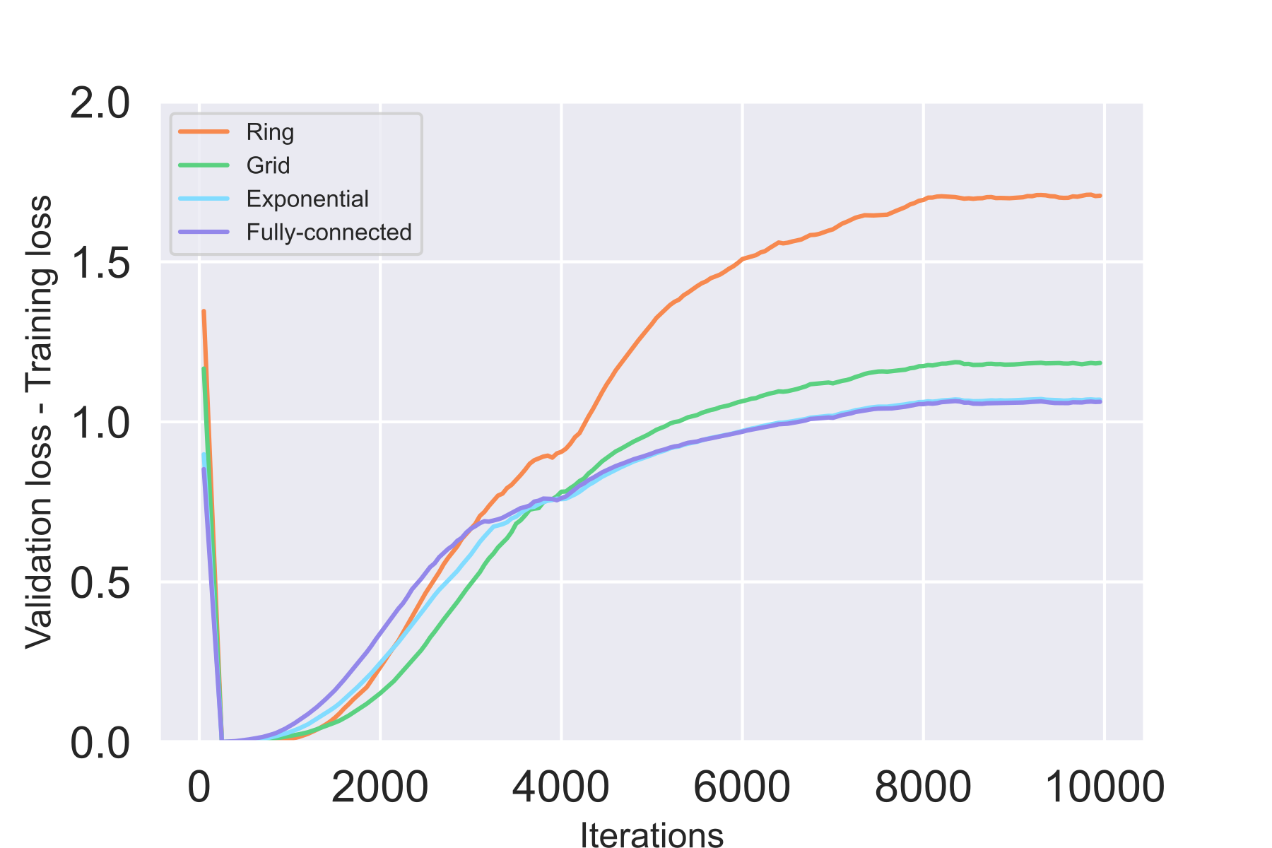
((d)) VGG-11 on CIFAR-10, 64 workers

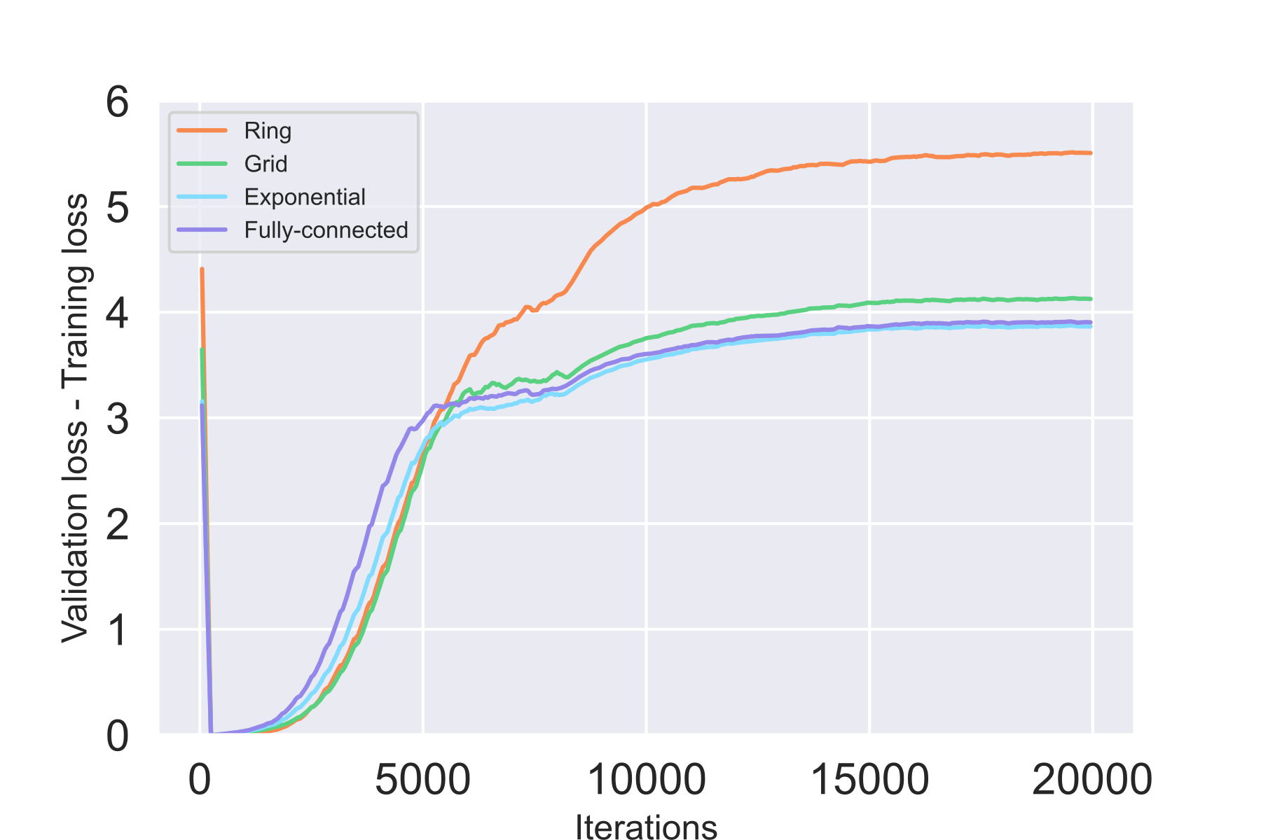
((e)) VGG-11 on CIFAR-100, 64 workers

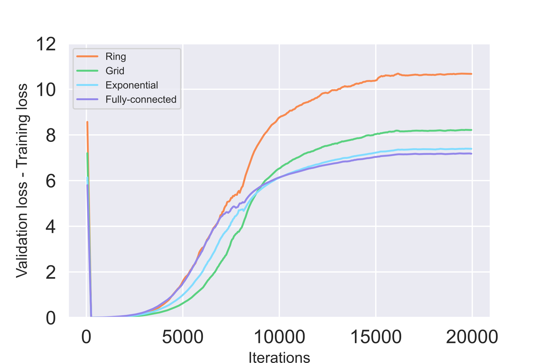
((f)) VGG-11 on Tiny ImageNet, 64 workers

Figure 3: Loss differences of training VGG-11 with D-SGD on different topologies.

5.1 Experimental Setup

Networks and datasets. Network architectures VGG-11 (Simonyan & Zisserman, 2014) and ResNet-18 (He et al., 2016b) are employed in our experiments. The models are trained on CIFAR-10, CIFAR-100 (Krizhevsky et al., 2009) and Tiny ImageNet (Le & Yang, 2015), three popular benchmark image classification datasets. The CIFAR-10 dataset consists of 60,000 32$\times$32 color images across 10 classes, with each class containing 5,000 training and 1,000 testing images. The CIFAR-100 dataset also consists of 60,000 32$\times$32 color images, except that it has 100 classes, each class containing 5,00 training and 1,00 testing images. Tiny ImageNet contains 120,000 64$\times$ 64 color images in 200 classes, each class containing 500 training images, 50 validation images, and 50 test images. No other pre-processing methods are employed.

Training setting. Vanilla D-SGD is employed to train image classifiers based on VGG-11 and ResNet-18 on fully-connected, ring, grid, and static exponential topologies. The number of workers is set as 32 and 64. Batch normalization (Ioffe & Szegedy, 2015) and dropout (Srivastava et al., 2014) are employed in training VGG-11. The local batch size is set as 64. To control the impact of different total batch size (local batch size $\times$ worker number) caused by the different number of workers, we apply the linear scaling law (i.e., linearly increase learning rate w.r.t. total batch size) (He et al., 2016a; Goyal et al., 2017). The initial learning rate is set as $0.4$ and will be divided by $10$ when the model has accessed $2/5$ and $4/5$ of the total number of iterations (He et al., 2016a). All other techniques, including momentum (Qian, 1999), weight decay (Tihonov, 1963), early stopping (Bengio, 2012) and data augmentation (LeCun et al., 1998) are disabled.

Implementations. All our experiments are conducted on a computing cluster with GPUs of NVIDIA^® Tesla^™ V100 16GB and CPUs of Intel^® Xeon^® Gold 6140 CPU @ 2.30GHz. Our code is implemented based on PyTorch (Paszke et al., 2019).

5.2 Communication topology and generalization

We calculate the difference between the validation loss and the training loss on different topologies separately, as shown in Figure 3 and Figure C.1. Two observations are obtained from those figures: (1) for large topologies, the loss differences can be sorted as follows: fully-connected $\approx$ exponential $<$ grid $<$ ring; (2) as the worker number increases, the loss differences of D-SGD on different topologies increase. These observations suggest that (1) D-SGD generalizes better on well-connected topology with a larger spectral gap; (2) the generalizability gap of D-SGD on different topologies grows as the worker number increases.

In comparison to ResNet-18, we observe when VGG-11 is chosen as the backbone, the generalization gaps between different topologies are larger (see Figure 3 and Figure C.1). We conjecture that the generalization gaps are amplified because the Hölder constant $L$ of VGG-11 is larger than that of ResNet-18, according to our theory suggesting that the generalization error of D-SGD linearly increases with $L$ (see Theorem 4).

One may observe that the loss difference of the fully-connected topology is larger than that of other topologies in the initial training phase, which seems to be inconsistent with our theory. Theoretically, explaining this phenomenon is an optimization problem, which is beyond the scope of this work. One possible explanation is motivated by the stability-convergence trade-off in iterative optimization algorithms (Chen et al., 2018). Since the fully-connected system converges faster, the corresponding optimization error is smaller than the other three kinds of systems at the beginning of training. Therefore, the fully-connected system is less stable in the initial phase of training.

6 Future Works

Implicit bias of D-SGD. As pointed out in Zhang et al. (2021), the additional gradient noise in D-SGD helps it converge to a flatter minima compared to centralized distributed SGD. Therefore, a direct question is whether there is a superior implicit bias effect (Soudry et al., 2018; Ji & Telgarsky, 2019; Arora et al., 2019; Wang et al., 2021) in D-SGD compared to centralized distributed SGD, which involves the convergence direction? Would decentralization change the implicit bias? Can we derive fine-grained generalization bounds of D-SGD based on the implicit bias analysis?

7 Conclusion

In this paper, we theoretically analyze the algorithmic stability and generalizability of decentralized stochastic gradient descent (D-SGD). We prove that the consensus model learned by D-SGD is $\mathcal{O}{(N^{-1}+m^{-1}+\lambda^{2})}$-stable, where $N$ is the total sample size on each worker, $m$ is the worker number, and $1-\lambda$ is the spectral gap of the communication topology. Based on this stability result, we obtain an $\mathcal{O}{(N^{-(1+\alpha)/2}+m^{-(1+\alpha)/2}+\lambda^{1+\alpha}+\phi_{\mathcal{S}})}$ in-average generalization bound, characterizing the gap between the training performance and the test performance. Our error bounds are non-vacuous, even when the worker number is sufficiently large, or the communication topology is sufficiently sparse. According to our theory, we can conclude: (1) the generalizability of D-SGD is positively correlated with the spectral gap of the underlying communication topology; (2) the generalizability of D-SGD decreases when the worker number increases. These theoretical findings are then empirically justified by the experiments of VGG-11 and ResNet-18 on CIFAR-10, CIFAR-100, and Tiny ImageNet. The theory can also explain why consensus control at the beginning of training is able to promote the generalizability of D-SGD.

Appendix A Additional Background

The following remarks clarify some notations in the literature.

Remark A.1.

Stochastic learning algorithms $A:\cup_{n}\mathcal{Z}^{n}\mapsto\mathcal{W}$ are often applied to produce an output model $A(\mathcal{S})\in\mathbb{R}^{d}$ based on the training set $\mathcal{S}$. To avoid ambiguity, let $A(\mathcal{S})$ denote the model generated by a general learning algorithm, and $\mathbf{w}$ denote the models generated by a specific stochastic learning algorithm.

Remark A.2.

Stochastic learning introduces two kinds of randomness: one from the sampling of training examples and another from the adopted randomized algorithm. In the following analysis, $\mathbb{E}_{A}[\cdot]$ stands for the expectation w.r.t. the randomness of the algorithm $A$, and $\mathbb{E}_{S}[\cdot]$ denotes the expectation w.r.t. the randomness originating from sampling the data set $\mathcal{S}$. Notice that $\mathcal{S}\sim\mathcal{D}^{n}$ and $z\sim\mathcal{D}$, therefore $\mathbb{E}_{\mathcal{S}}[\cdot]$ differs from $\mathbb{E}_{z}[\cdot]$ defined in Section 3.

Based on the work by Hardt et al. (2016) and Bottou & Bousquet (2008), we give a formulation of excess error decomposition and demonstrate how to understand generalization through error decomposition.

Definition A.1 (Excess Error Decomposition).

We denote the empirical risk minimization (ERM) solution by $\mathbf{w}_{\mathcal{S}}^{*}=\arg\min_{\mathbf{w}}F_{\mathcal{S}}(\mathbf{w})$ and $\mathbf{w}^{*}=\arg\min_{\mathbf{w}}F(\mathbf{w})$. The excess error $F(A(\mathcal{S}))-F(\mathbf{w}^{*})$ can be decomposed as

$$\underbrace{\mathbb{E}_{\mathcal{S},A}\left[F(A(\mathcal{S}))-F\left(\mathbf{w}^{*}\right)\right]}_{\text{Excess error }}\\ =\underbrace{\mathbb{E}_{\mathcal{S},A}\left[F(A(\mathcal{S}))-F_{\mathcal{S}}(A(\mathcal{S}))\right]}_{\text{Generalization error}}+\underbrace{\mathbb{E}_{\mathcal{S},A}\left[F_{\mathcal{S}}(A(\mathcal{S}))-F_{\mathcal{S}}\left(\mathbf{w}_{\mathcal{S}}^{*}\right)\right]}_{{\text{Optimization error }}}+\mathbb{E}_{\mathcal{S},A}\left[F_{\mathcal{S}}(\mathbf{w}_{\mathcal{S}}^{*})-F\left(\mathbf{w}^{*}\right)\right]\\ \leq\underbrace{\mathbb{E}_{\mathcal{S},A}\left[F(A(\mathcal{S}))-F_{\mathcal{S}}(A(\mathcal{S}))\right]}_{\text{Generalization error}}+\underbrace{\mathbb{E}_{\mathcal{S},A}\left[F_{\mathcal{S}}(A(\mathcal{S}))-F_{\mathcal{S}}\left(\mathbf{w}_{\mathcal{S}}^{*}\right)\right]}_{{\text{Optimization error }}}$$ (A.1)

The last inequality holds since and $\mathbb{E}_{\mathcal{S},A}\left[F_{\mathcal{S}}(\mathbf{w}_{\mathcal{S}}^{*})\right]\leq\mathbb{E}_{\mathcal{S},A}\left[F_{\mathcal{S}}\left(\mathbf{w}^{*}\right)\right]=\mathbb{E}_{\mathcal{S}}\big{[}F(\mathbf{w}^{*})$. The empirical risk and the population risk above are defined in Section 3. This paper considers upper bounding the first term called the generalization error.

Lipschitzness and smoothness are two commonly adopted assumptions to establish the uniform stability guarantees of SGD.

Assumption A.1 (Lipschitzness).

$\big{\|}\nabla f(\mathbf{w};z)\big{\|}_{2}\leq G$ for all $\mathbf{w}\in\mathbb{R}^{d}$ and $z\in\mathcal{Z}$.

Assumption A.2 (Smoothness).

$f$ is $\beta$-smooth if for any $z$ and $\mathbf{w},\widetilde{\mathbf{w}}\in\mathbb{R}^{d}$,

$$\big{\|}\nabla f(\mathbf{w};z)-\nabla f(\widetilde{\mathbf{w}};z)\big{\|}_{2}\leq\beta\|\mathbf{w}-\widetilde{\mathbf{w}}\|_{2}.$$ (A.2)

These two restrictive assumptions are not satisfied in many real contexts. For example, the Lipschitz constant $G$ can be very large for some learning problems (Fazlyab et al., 2019; Lei & Ying, 2020). In addition, neural nets with piecewise linear activation functions like ReLU are not smooth. Smoothness is generally difficult to ensure at the beginning and intermediate phases of deep neural network training (Bassily et al., 2020).

Assumption A.3 (Hölder Continuity).

Let $L>0,\alpha\in[0,1]$. $\nabla f(\cdot,z)$ is $(\alpha,L)$-Hölder continuous if for all $\mathbf{w},\widetilde{\mathbf{w}}\in\mathbb{R}^{d}$ and $z\in\mathcal{Z}$,

$$\big{\|}\nabla f(\mathbf{w};z)-\nabla f(\widetilde{\mathbf{w}};z)\big{\|}_{2}\leq L\|\mathbf{w}-\widetilde{\mathbf{w}}\|_{2}^{\alpha}.$$ (A.3)

Hölder continuous gradient assumption is much weaker than smoothness by definition. Serving as an intermediate class of functions $(C^{1,\alpha}\left(\mathbb{R}^{n}\right))$ between smooth functions $(C^{1,1}\left(\mathbb{R}^{n}\right))$ and functions with Lipschitz continuous gradients $(C^{1,0}\left(\mathbb{R}^{n}\right))$, the main advantage of functions with Hölder continuous gradients lies in the ability to automatically adjust the smoothness parameter to a proper level (Nesterov, 2015): Eq. A.3 with $\alpha=1$ corresponds to smoothness and Eq. A.3 with $\alpha=0$ is equivalent to Lipschitzness (see Assumption A.1).

Assumption A.4 (Gaussian Weight Difference).

We assume that the difference between $\mathbf{w}_{k}^{(t)}$ and $\widetilde{\mathbf{w}}_{k}^{(t)}$ (the $t$-th iterate on $k$-th worker produced by Eq. 1 based on $\mathcal{S}_{k}$ and $\mathcal{S}_{k}^{(i)}$ respectively) is independent and normally distributed:

$$\big{(}\mathbf{w}_{k}^{(t)}-\widetilde{\mathbf{w}}_{k}^{(t)}\big{)}{\sim}\mathcal{N}(\mu_{t,k},\sigma_{t,k}^{2}I_{d}),\quad k=1,\dots,m$$

where $I_{d}$ denotes an identity matrix with size $d$, and $\mu_{t,k},\sigma_{t,k}^{2}$ are unknown parameters. We also give a mild constraint that the $d$-dimensional parameter $\mu_{t,k}$ satisfies $d\cdot\mu_{0}^{2}\leq\|\mu_{t,k}\|_{2}^{2}\leq d\cdot\mu^{2}$ and the parameter $\sigma_{t,k}^{2}\in\mathbb{R}$ is bounded by $\sigma^{2}$. Assumption A.4 is mild since $\mathcal{S}_{k}$ and $\mathcal{S}_{k}^{(i)}$ only vary at one point.

Commonly used stability notions are listed below.

Definition A.2 (Hypothesis Stability).

A stochastic algorithm $A$ is hypothesis $\epsilon$-stable w.r.t. the loss function $f$ if for all training data sets $\mathcal{S},\mathcal{S}^{(i)}\in\mathcal{Z}^{n}$ that differ by at most one example, we have

$$\mathbb{E}_{z}\mathbb{E}_{A}\big{[}f(A(\mathcal{S});z)-f(A(\mathcal{S}^{(i)});z)\big{]}\leq\epsilon.$$ (A.4)

Definition A.3 (Uniform Stability).

A stochastic algorithm $A$ is $\epsilon$-uniformly stable w.r.t. the loss function $f$ if for all training data sets $\mathcal{S},\mathcal{S}^{(i)}\in\mathcal{Z}^{n}$ that differ by at most one example, we have

$$\sup_{z}\mathbb{E}_{A}\big{[}f(A(\mathcal{S});z)-f(A(\mathcal{S}^{(i)});z)\big{]}\leq\epsilon.$$ (A.5)

Definition A.4 (On-average Model Stability, (Lei & Ying, 2020)).

A stochastic algorithm $A$ is $\ell_{2}$ on-average model $\epsilon$-stable for all training data sets $\mathcal{S},\mathcal{S}^{(i)}\in\mathcal{Z}^{n}$ that differ by at most one example, we have

$$\frac{1}{N}\sum_{i=1}^{N}\mathbb{E}_{\mathcal{S},\mathcal{S}^{(i)},A}\big{[}\|A(\mathcal{S})-A(\mathcal{S}^{(i)})\|_{2}^{2}\big{]}\leq\epsilon^{2}.$$

Some widely used notions regarding decentralized training are listed as follows.

Definition A.5 (Doubly Stochastic Matrix).

Let $\mathcal{G}=(\mathcal{V},\mathcal{E})$ stand for the decentralized communication topology where $\mathcal{V}$ denotes the set of m computational nodes and $\mathcal{E}$ represents the edge set. For any given graph $\mathcal{G}=(\mathcal{V},\mathcal{E})$, the doubly stochastic gossip matrix ${\mathbf{P}}=[\mathbf{P}_{k,l}]\in\mathbb{R}^{m\times m}$ is defined on the edge set $\mathcal{E}$ that satisfies: (1) If $k\neq l$ and $(k,l)\notin{\cal E}$, then $\mathbf{P}_{k,l}=0$ (disconnected); otherwise, $\mathbf{P}_{k,l}>0$ (connected); (2) $\mathbf{P}_{k,l}\in[0,1]\ \forall k,l$; (3) ${\mathbf{P}}={\mathbf{P}}^{\top}$; and (4) $\sum_{k}\mathbf{P}_{k,l}=\sum_{l}\mathbf{P}_{k,l}=1$ (standard weight matrix for undirected graph).

Definition A.6 (Spectral Gap).

Denote $\lambda=\max\left\{\left|\lambda_{2}\right|,\left|\lambda_{m}\right|\right\}$ where $\lambda_{i}\ (i=2,\dots,m)$ is the $i$-th largest eigenvalue of gossip matrix ${\mathbf{P}}\in\mathbb{R}^{m\times m}$. The spectral gap of a gossip matrix $\mathbf{P}$ can be defined as follows:

$${\text{s}pectral\ gap}:=1-\lambda.$$

According to the definition of doubly stochastic matrix (Definition A.5), we have $0\leq\lambda<1$. The spectral gap measures the connectivity of the communication topology, which is close to 0 for sparse topologies and will approach 1 for well-connected topologies.

To facilitate our subsequent analysis, we provide some preliminaries of matrix algebra here.

Definition A.7 (Frobenius Norm).

The Frobenius norm (Euclidean norm, or Hilbert–Schmidt norm) is the matrix norm of a matrix $\mathbf{A}\in\mathbb{R}^{p\times q}$ defined as the square root of the sum of the squares of its elements:

$$\|\mathbf{A}\|_{F}=\sqrt{\sum_{i=1}^{q}\sum_{j=1}^{q}\left|a_{ij}\right|^{2}}=\sqrt{\operatorname{Tr}(\mathbf{A}^{\mkern-1.5mu\mathsf{T}}\mathbf{A})}.$$

For any $\mathbf{A},\mathbf{B}\in\mathbb{R}^{p\times q}$, the following identity holds:

$$\|\mathbf{A}+\mathbf{B}\|_{\text{F}}^{2}=\|\mathbf{A}\|_{\text{F}}^{2}+\|\mathbf{B}\|_{\text{F}}^{2}+2\langle\mathbf{A},\mathbf{B}\rangle_{F},$$

where $\langle\cdot,\cdot\rangle_{\text{F}}$ is the Frobenius inner product.

Appendix B Additional Related Work

B.1 Non-centralized learning.

To handle an increasing amount of data and model parameters, distributed learning across multiple computing nodes (workers) emerges. A traditional distributed learning system usually follows a centralized setup (Abadi et al., 2016). However, such a central server-based learning scheme suffers from two main issues: (1) A centralized communication protocol significantly slows down the training since central servers are easily overloaded, especially in low-bandwidth or high-latency cases (Lian et al., 2017); (2) There exists potential information leakage through privacy attacks on model parameters despite decentralizing data using federated learning (Zhu et al., 2019; Geiping et al., 2020; Yin et al., 2021). As an alternative, training in a non-centralized fashion allows workers to balance the load on the central server through the gossip technique, as well as maintain confidentiality (Warnat-Herresthal et al., 2021). Model decentralization can be divided into three kinds of categories by layers (Lu & De Sa, 2021): (1) On the application layer, decentralized training usually refers to federated learning (Zhao et al., 2018; Dai et al., 2022) ; (2) On the protocol layer, decentralization denotes average gossip where local workers communicate by averaging their parameters with their neighbors on a graph (Lian et al., 2017) and (3) on the topology layer, it means a sparse topology graph (Wan et al., 2020).

B.2 Generalization via algorithmic stability.

Algorithmic stability theory, PAC-Bayes theory, and information theory are major tools for constructing algorithm-dependent generalization bounds (Neu et al., 2021). A direct intuition behind algorithmic stability is that if an algorithm does not rely excessively on any single data point, it can generalize well. Proving generalization bounds based on the sensitivity of the algorithm to changes in the learning sample can be traced back to Vapnik & Chervonenkis (1974) and Devroye & Wagner (1979). After that, the celebrated work by Bousquet & Elisseeff (2002) establishes the relationship between uniform stability and generalization in high probability. Follow-up work by Shalev-Shwartz et al. (2010) identifies stability as the major necessary and sufficient condition for learnability. Then, Hardt et al. (2016) provide uniform stability bounds for stochastic gradient methods (SGM) and show the strong stability properties of SGD with convex and smooth losses. Recent work by Lei & Ying (2020) defines a new on-average stability notion and conducts generalization analyses on SGD with the Hölder continuous assumption. In addition to uniform stability, there are other stability notions including on-average stability (Shalev-Shwartz et al., 2010), uniform argument stability (Liu et al., 2017), data-dependent stability (Kuzborskij & Lampert, 2018), hypothesis set stability (Foster et al., 2019) and locally elastic stability (Deng et al., 2021).

Appendix C Additional Experimental Results

We also calculate the difference between the validation loss and the training loss of training ResNet-18 with D-SGD.

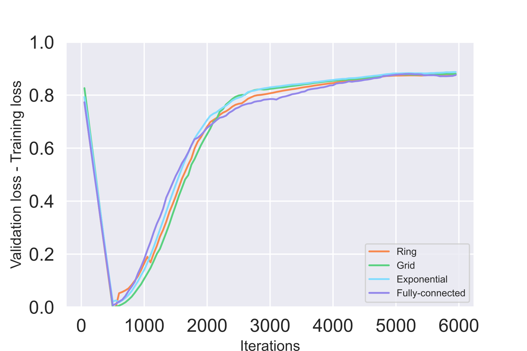
((a)) CIFAR-10, 32 workers

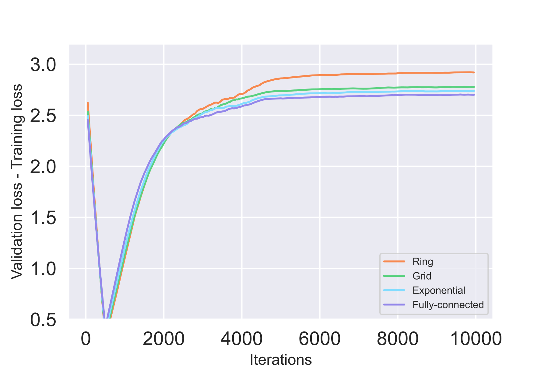
((b)) CIFAR-100, 32 workers

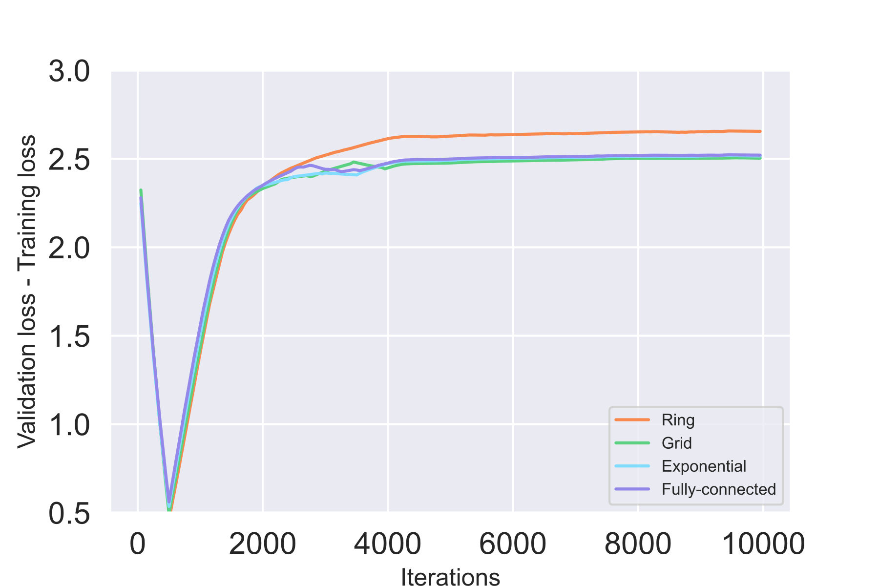
((c)) Tiny ImageNet, 32 workers

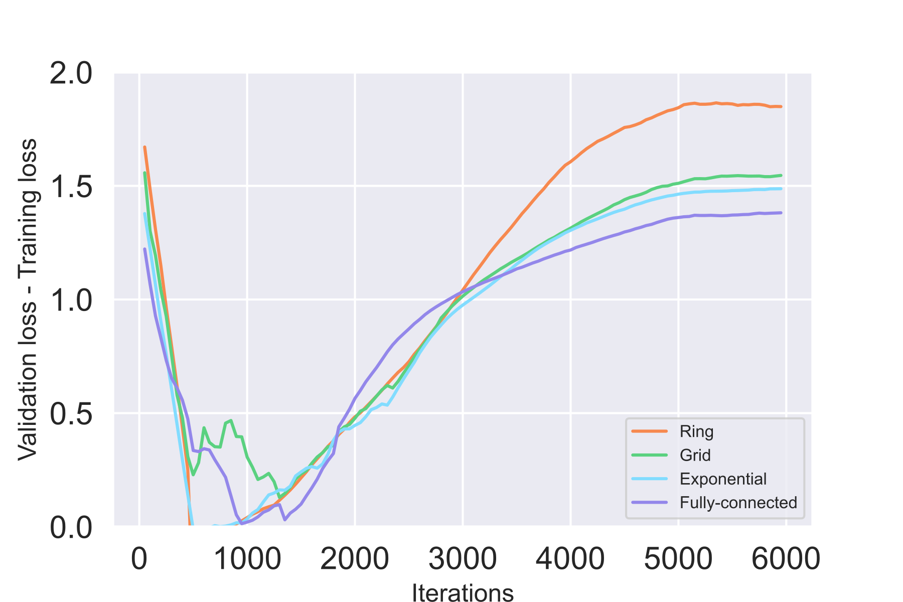
((d)) CIFAR-10, 64 workers

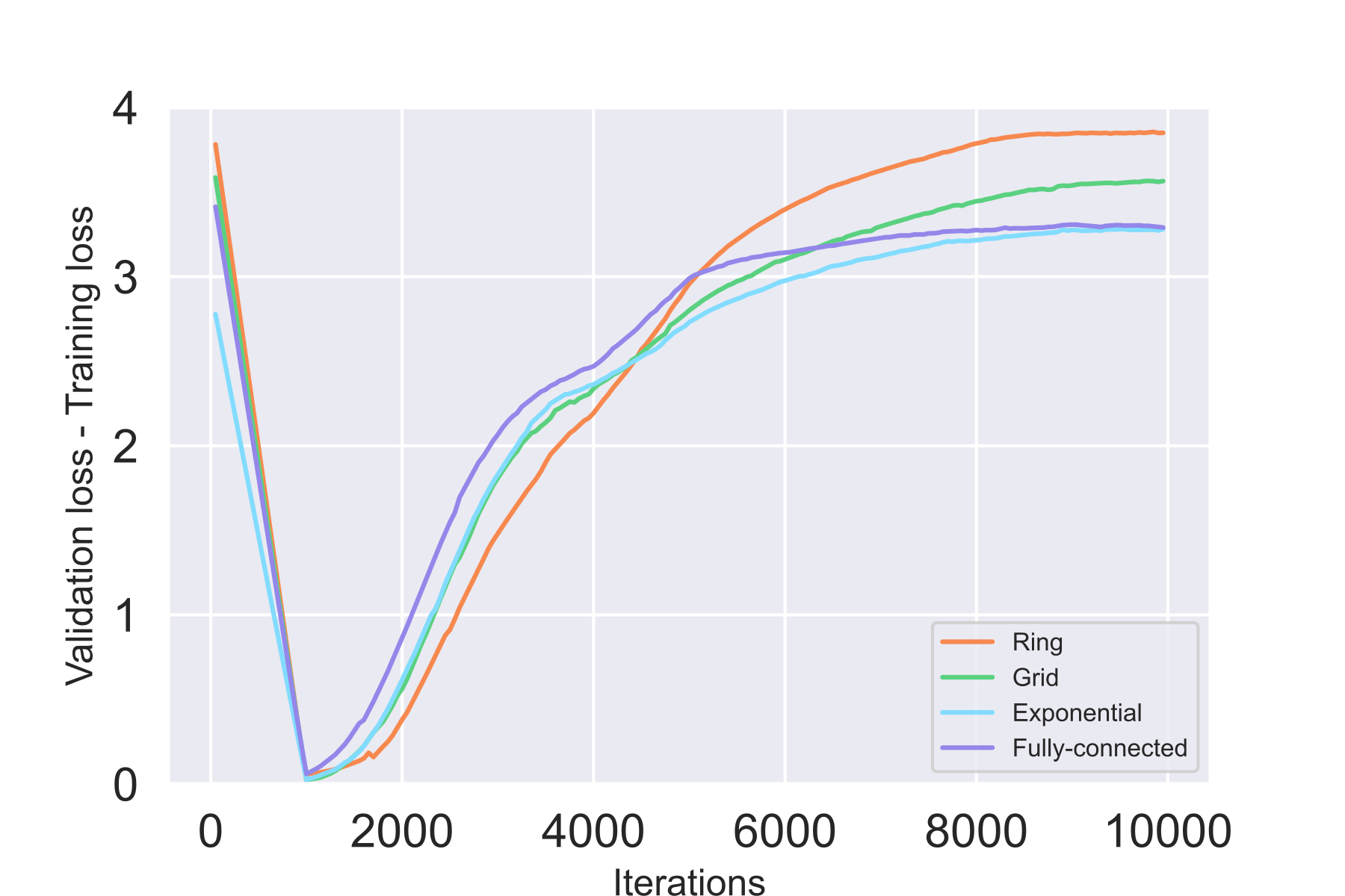
((e)) CIFAR-100, 64 workers

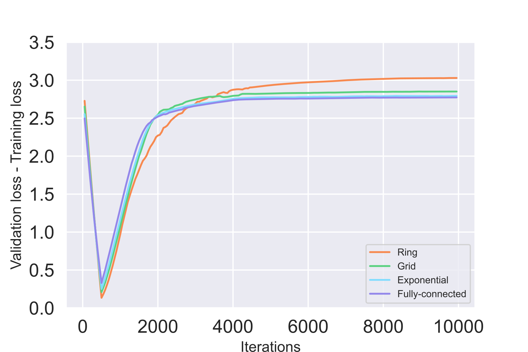
((f)) Tiny ImageNet, 64 workers

Figure C.1: Loss differences of training ResNet-18 with D-SGD on different topologies.

Appendix D Proof

D.1 Technical lemmas

To complete our proof, we first introduce some technical lemmas.

Lemma D.1 (Corollary 1.14., (Montenegro & Tetali, 2006)).

Let $\mathbf{M}$ stand for the matrix with all the elements be $1/m$ and $\mathbf{P}$ is defined in Definition A.5. For any $k\in\mathbb{Z}^{+}$, the following inequality holds:

$$\left\|\mathbf{P}^{k}-\mathbf{M}\right\|_{2,2}\leq\left\|\mathbf{P}\right\|^{k}_{\lambda}.$$ (D.1)

Lemma D.2.

For any $a,b\in\mathbb{R}$ and $p\in\mathbb{R}^{+}$, the following inequality holds:

$$(a+b)^{2}\leq(1+p)a^{2}+(1+p^{-1})b^{2}.$$ (D.2)

Lemma D.3 (Self-bounding Property, (Lei & Ying, 2020)).

Assume that for all $z\in\mathcal{Z}$, the map $\mathbf{w}\mapsto f(\mathbf{w};z)$ is nonnegative with its gradient $\nabla f(\mathbf{w};z)$ being $(\alpha,L)$-Hölder continuous (Assumption A.3), then $\mathbf{w}\mapsto f(\mathbf{w};z)$ can be bounded as

$$\|\nabla f(\mathbf{w},z)\|_{2}\leq c_{\alpha,1}f^{\frac{\alpha}{1+\alpha}}(\mathbf{w},z),\quad\forall\mathbf{w}\in\mathbb{R}^{d},z\in\mathcal{Z}.$$

where

$$c_{\alpha,1}=\begin{cases}(1+1/\alpha)^{\frac{\alpha}{1+\alpha}}L^{\frac{1}{1+\alpha}},&\mbox{if }\alpha>0\\ \sup_{z}\|\nabla f(0;z)\|_{2}+L,&\mbox{if }\alpha=0.\end{cases}$$ (D.3)

Remark D.1.

The self-binding property implies that H”older continuous gradients can be controlled by function values. The $\alpha=1$ and $\alpha\in(0,1)$ case are established by Srebro et al. (2010) and Ying & Zhou (2017), respectively. The case where $\alpha=0$ follows directly from Assumption A.3.

Lemma D.4.

For any $a,b\in\mathbb{R}^{d}$ with $a_{i}$, $b_{i}$ being their $i$-th components, respectively, the following inequality holds:

$$a^{\mkern-1.5mu\mathsf{T}}b=\sum_{i}a_{i}b_{i}\leq\sqrt{\sum_{i}a_{i}^{2}\sum_{i}b_{i}^{2}}\leq\frac{\sum_{i}a_{i}^{2}+\sum_{i}b_{i}^{2}}{2}.$$ (D.4)

Lemma D.5.

Let $x,y\in\mathbb{R}^{d}$, for any differentiable function $h\ (\mathbb{R}^{d}\mapsto\mathbb{R})$ which has $(\alpha,L)$-Hölder continuous gradient, we have

$$h(x)-h(y)\leq\frac{L}{1+\alpha}{\|x-y\|}_{2}^{1+\alpha}+\frac{1}{2}\|x-y\|^{2}_{2}+\frac{1}{2}\|\nabla h(y)\|^{2}_{2}.$$ (D.5)

Proof of Lemma D.5.

According to the definition of derivative, the difference between $h(x)$ and $h(y)$ can be written as

$$h(x)-h(y)=\int_{0}^{1}\langle\nabla h(u_{(t)}),x-y\rangle\mathrm{d}t,$$

where $u_{(t)}=y+t(x-y).$

Subtracting both sides with $\langle\nabla h(u_{(t)}),x-y\rangle$ gives

$$h(x)-h(y)-\langle\nabla h(y),x-y\rangle=\int_{0}^{1}\langle\nabla h(u_{(t)})-\nabla h(y),x-y\rangle\mathrm{d}t.$$

The triangle inequality and the $(\alpha,L)$-Hölder continuity of $h$ further guarantee

$$|h(x)-h(y)| =\int_{0}^{1}|\langle\nabla h(u_{(t)})-\nabla h(y),x-y\rangle|\mathrm{d}t+|\langle\nabla h(y),x-y\rangle|$$

$$\leq\int_{0}^{1}\|\nabla h(u_{(t)})-\nabla h(y)\|\|x-y\|\mathrm{d}t+|\langle\nabla h(y),x-y\rangle|$$

$$\leq\int_{0}^{1}L\|u_{(t)}-y\|^{\alpha}\|x-y\|\mathrm{d}t+|\langle\nabla h(y),x-y\rangle|$$

$$\leq L\|x-y\|^{1+\alpha}\int_{0}^{1}t^{\alpha}\mathrm{d}t+|\langle\nabla h(y),x-y\rangle|,$$

Since $|\langle\nabla h(y),x-y\rangle|\leq\frac{1}{2}\|x-y\|^{2}_{2}+\frac{1}{2}\|\nabla h(y)\|^{2}_{2}$, we arrive at

$$h(x)-h(y) \leq\frac{L}{1+\alpha}{\|x-y\|}_{2}^{1+\alpha}+|\langle\nabla h(y),x-y\rangle|$$

$$\leq\frac{L}{1+\alpha}{\|x-y\|}_{2}^{1+\alpha}+\frac{1}{2}\|x-y\|^{2}_{2}+\frac{1}{2}\|\nabla h(y)\|^{2}_{2}.$$

∎

D.2 Algorithmic stability of D-SGD

Proof of Theorem 1.

To begin with, we decompose $\sum_{k=1}^{m}\big{\|}\mathbf{w}_{k}^{(t+1)}-\widetilde{\mathbf{w}}_{k}^{(t+1)}\big{\|}_{2}^{2}$, the on-average stability of D-SGD at the $t$-th iteration, into three parts by the definition of the vector 2-norm. In the following, we will let $z_{k,\zeta_{t}}^{(t)}$ and $\tilde{z}_{k,\zeta_{t}}^{(t)}$ denote two random data points drawn from $\mathcal{S}_{k}$ and $\mathcal{S}^{(i)}_{k}$ on the $k$-th worker at the $i$-th iteration, respectively.

$$\sum_{k=1}^{m} \big{\|}\mathbf{w}_{k}^{(t+1)}-\widetilde{\mathbf{w}}_{k}^{(t+1)}\big{\|}_{2}^{2}$$

$$=\sum_{k=1}^{m}\big{\|}\sum_{l=1}^{m}\mathbf{P}_{k,l}\mathbf{w}_{t}(l)-\eta_{t}\nabla f\left(\mathbf{w}_{k}^{(t)};z_{k,\zeta_{t}}^{(t)}\right)-\sum_{l=1}^{m}\mathbf{P}_{k,l}\widetilde{\mathbf{w}}_{l}^{(t)}+\eta_{t}\nabla f\left(\widetilde{\mathbf{w}}_{k}^{(t)},\tilde{z}_{k,\zeta_{t}}^{(t)}\right)\big{\|}_{2}^{2}$$

$$=\sum_{k=1}^{m}\big{\|}\sum_{l=1}^{m}\mathbf{P}_{k,l}(\mathbf{w}_{l}^{(t)}-\widetilde{\mathbf{w}}_{l}^{(t)})\big{\|}_{2}^{2}+\sum_{k=1}^{m}{\eta_{t}}^{2}\big{\|}\nabla f\left(\mathbf{w}_{k}^{(t)};z_{k,\zeta_{t}}^{(t)}\right)-\nabla f\left(\widetilde{\mathbf{w}}_{k}^{(t)},\tilde{z}_{k,\zeta_{t}}^{(t)}\right)\big{\|}_{2}^{2}$$

$$-2\sum_{k=1}^{m}\eta_{t}\big{\langle}\sum_{l=1}^{m}\mathbf{P}_{k,l}(\mathbf{w}_{l}^{(t)}-\widetilde{\mathbf{w}}_{l}^{(t)}),\nabla f\left(\mathbf{w}_{k}^{(t)};z_{k,\zeta_{t}}^{(t)}\right)-\nabla f\left(\widetilde{\mathbf{w}}_{k}^{(t)},\tilde{z}_{k,\zeta_{t}}^{(t)}\right)\big{\rangle}$$

$$=\underbrace{\big{\|}\mathbf{P}(\mathbf{W}^{(t)}-\widetilde{\mathbf{W}}^{(t)})\big{\|}_{F}^{2}}_{\text{$T_{1}$}}+\underbrace{\sum_{k=1}^{m}\mathds{1}_{z_{k,\zeta_{t}}^{(t)}\neq\tilde{z}_{k,\zeta_{t}}^{(t)}}\big{[}\big{\|}\mathbf{w}_{k}^{(t+1)}-\widetilde{\mathbf{w}}_{k}^{(t+1)}\big{\|}_{2}^{2}-\big{\|}\sum_{l=1}^{m}\mathbf{P}_{k,l}(\mathbf{w}_{l}^{(t)}-\widetilde{\mathbf{w}}_{l}^{(t)})\big{\|}_{2}^{2}\big{]}}_{\text{$T_{2}$}}$$

$$+\sum_{k=1}^{m}\mathds{1}_{z_{k,\zeta_{t}}^{(t)}=\tilde{z}_{k,\zeta_{t}}^{(t)}}\big{[}{\eta_{t}}^{2}\big{\|}\nabla f\left(\mathbf{w}_{k}^{(t)};z_{k,\zeta_{t}}^{(t)}\right)-\nabla f\left(\widetilde{\mathbf{w}}_{k}^{(t)},\tilde{z}_{k,\zeta_{t}}^{(t)}\right)\big{\|}_{2}^{2}$$

$$\underbrace{\qquad\qquad\qquad\qquad\quad\quad\ \ -2\eta_{t}\big{\langle}\sum_{l=1}^{m}\mathbf{P}_{k,l}(\mathbf{w}_{l}^{(t)}-\widetilde{\mathbf{w}}_{l}^{(t)}),\nabla f\left(\mathbf{w}_{k}^{(t)};z_{k,\zeta_{t}}^{(t)}\right)-\nabla f\left(\widetilde{\mathbf{w}}_{k}^{(t)},\tilde{z}_{k,\zeta_{t}}^{(t)}\right)\big{\rangle}\big{]}}_{\text{$T_{3}$}}$$

where $\left\|\cdot\right\|_{F}$ denotes the Frobenius norm (see Definition A.7).

(1) To construct our proof, we start by constructing an upper bound of $\mathbb{E}_{A}(T_{1})$:

$$\mathbb{E}_{A}(T_{1})=\mathbb{E}_{A}\big{[}\big{\|}\mathbf{P}(\mathbf{W}^{(t)}-\widetilde{\mathbf{W}}^{(t)})\big{\|}_{F}^{2}\leq d(\sigma^{2}+\mu^{2})\big{[}(m-1)\lambda^{2}+1\big{]}.$$ (D.6)

Proof.

The on-averaged stability after a single gossip communication can be written as

$$\big{\|}\mathbf{P}(\mathbf{W}^{(t)}-\widetilde{\mathbf{W}}^{(t)})\big{\|}_{F}^{2} =\sum_{k=1}^{m}\big{\|}\sum_{l=1}^{m}\mathbf{P}_{k,l}(\mathbf{w}_{l}^{(t)}-\widetilde{\mathbf{w}}_{l}^{(t)})\big{\|}_{2}^{2}=\sum_{v=1}^{d}\sum_{k=1}^{m}\big{\|}\sum_{l=1}^{m}\mathbf{P}_{k,l}(\mathbf{w}_{l}^{v,(t)}-\widetilde{\mathbf{w}}_{l}^{v,(t)})\big{\|}_{2}^{2}$$

$$=\sum_{v=1}^{d}\sum_{k=1}^{m}\sigma_{t,k}^{2}(\sum_{l=1}^{m}\mathbf{P}_{k,l}^{2})\{\frac{\sum_{l=1}^{m}\mathbf{P}_{k,l}[(\mathbf{w}_{l}^{v,(t)}-\widetilde{\mathbf{w}}_{l}^{v,(t)})-\mu_{t,k}^{v}]+\sum_{l=1}^{m}\mathbf{P}_{k,l}\mu_{t,l}^{v}]}{\sigma_{t,k}\sqrt{\sum_{l=1}^{m}\mathbf{P}_{k,l}^{2}}}\}^{2}$$

$$\leq\sum_{v=1}^{d}\sum_{k=1}^{m}\sigma_{t,k}^{2}(\sum_{l=1}^{m}\mathbf{P}_{k,l}^{2})\{\frac{\sum_{l=1}^{m}\mathbf{P}_{k,l}[(\mathbf{w}_{l}^{v,(t)}-\widetilde{\mathbf{w}}_{l}^{v,(t)})-\mu_{t,k}^{v}]}{\sigma_{t,k}\sqrt{\sum_{l=1}^{m}\mathbf{P}_{k,l}^{2}}}\}^{2}+\mu^{2}dm\cdot\sum_{k=1}^{m}\sum_{l=1}^{m}\mathbf{P}_{k,l}^{2}$$

$$+\sum_{v=1}^{d}\sum_{k=1}^{m}(\sum_{l=1}^{m}\mathbf{P}_{k,l}^{2})\frac{\sum_{l_{1}=1}^{m}\sum_{l_{2}=1}^{m}\mathbf{P}_{k,l_{1}}\mathbf{P}_{k,l_{2}}\mu_{t,l_{1}}^{v}[(\mathbf{w}_{l_{1}}^{v,(t)}-\widetilde{\mathbf{w}}_{l_{1}}^{v,(t)})-\mu_{t,l_{1}}^{v}]}{\sqrt{\sum_{l_{1}=1}^{m}\mathbf{P}_{k,l}^{2}}\sqrt{\sum_{l_{2}=1}^{m}\mathbf{P}_{k,l}^{2}}},$$ (D.7)

where $\mathbf{w}_{l}^{v,(t)}$ and $\widetilde{\mathbf{w}}_{l}^{v,(t)}$ stacks the $v$-th entry of the $d$-dimensional vector $\mathbf{w}_{l}^{(t)}$ and $\widetilde{\mathbf{w}}_{l}^{(t)}$, respectively. The last inequality holds since $\sum_{v=1}^{d}(\mu_{t,l}^{v})^{2}\leq d\mu^{2}$.

Since the weight difference is normally distributed:

$$\big{(}\mathbf{w}_{k}^{(t)}-\widetilde{\mathbf{w}}_{k}^{(t)}\big{)}\sim\mathcal{N}(\mu_{t,k},\sigma_{t,k}^{2}I_{d}),\quad k=1,\dots,m,$$

with $\mu_{t,k}$ satisfying $\|\mu_{t,k}\|_{2}^{2}\leq d\cdot\mu^{2}$ and $\sigma_{t,k}^{2}\in\mathbb{R}$ being bounded by $\sigma^{2}$, we obtain

$$\frac{\sum_{l=1}^{m}\mathbf{P}_{k,l}[(\mathbf{w}_{l}^{v,(t)}-\widetilde{\mathbf{w}}_{l}^{v,(t)})-\mu_{t,k}^{v}]}{\sigma_{t,k}\sqrt{\sum_{l=1}^{m}\mathbf{P}_{k,l}^{2}}}\stackrel{{\scriptstyle i.i.d.}}{{\sim}}\mathcal{N}(0,1),\quad l=1,\dots,m.$$

Since the sum of squared i.i.d. standard normal variables follows a Chi-Square distribution with 1 degree of freedom, we arrive at

$$\{\frac{\sum_{l=1}^{m}\mathbf{P}_{k,l}[(\mathbf{w}_{l}^{v,(t)}-\widetilde{\mathbf{w}}_{l}^{v,(t)})-\mu_{t,k}^{v}]}{\sigma_{t,k}\sqrt{\sum_{l=1}^{m}\mathbf{P}_{k,l}^{2}}}\}^{2}{\sim}\mathcal{X}^{2}{(1)},\quad l=1,\dots,m.$$

Furthermore, since $\forall l$ $\mathbb{E}_{A}[(\mathbf{w}_{l}^{v,(t)}-\widetilde{\mathbf{w}}_{l}^{v,(t)})-\mu_{t,l}^{v}]=0$, we have

$$\mathbb{E}_{A}\left[\sum_{v=1}^{d}\sum_{k=1}^{m}(\sum_{l=1}^{m}\mathbf{P}_{k,l}^{2})\frac{\sum_{l_{1}=1}^{m}\sum_{l_{2}=1}^{m}\mathbf{P}_{k,l_{1}}\mathbf{P}_{k,l_{2}}\mu_{t,l_{1}}^{v}[(\mathbf{w}_{l_{1}}^{v,(t)}-\widetilde{\mathbf{w}}_{l_{1}}^{v,(t)})-\mu_{t,l_{1}}^{v}]}{\sqrt{\sum_{l_{1}=1}^{m}\mathbf{P}_{k,l}^{2}}\sqrt{\sum_{l_{2}=1}^{m}\mathbf{P}_{k,l}^{2}}}\right]=0.$$

As a consequence,

$$\mathbb{E}_{A}\big{[}\big{\|}\mathbf{P}(\mathbf{W}^{(t)}-\widetilde{\mathbf{W}}^{(t)})\big{\|}_{F}^{2}\leq d\sigma^{2}\sum_{k=1}^{m}\lambda_{k}^{2}+d\mu^{2}\sum_{k=1}^{m}\lambda_{k}^{2}\leq d(\sigma^{2}+\mu^{2})[1+(m-1)\lambda^{2}],$$

where $1-\lambda$ is the spectral gap of the communication topology.

(2) For the second part $T_{2}$, we have

$$T_{2}\leq\sum_{k=1}^{m}\mathds{1}_{z_{k,\zeta_{t}}^{(t)}\neq\tilde{z}_{k,\zeta_{t}}^{(t)}}p\big{\|}\sum_{l=1}^{m}\mathbf{P}_{k,l}(\mathbf{w}_{l}^{(t)}\scalebox{0.75}[1.0]{$-$}\widetilde{\mathbf{w}}_{l}^{(t)})\big{\|}_{2}^{2}\scalebox{0.75}[1.0]{$+$}\sum_{k=1}^{m}\mathds{1}_{z_{k,\zeta_{t}}^{(t)}\neq\tilde{z}_{k,\zeta_{t}}^{(t)}}(1+p^{-1})c_{\alpha,1}^{2}{\eta_{t}}^{2}\big{(}f^{\frac{2\alpha}{1+\alpha}}(\mathbf{w}_{k}^{(t)};z_{k,\zeta_{t}}^{(t)})\scalebox{0.75}[1.0]{$+$}f^{\frac{2\alpha}{1+\alpha}}(\widetilde{\mathbf{w}}_{k}^{(t)},\tilde{z}_{k,\zeta_{t}}^{(t)})\big{)}.$$ (D.8)

Proof.

Eq. D.8 are mainly based on Lemma D.2 and Lemma D.3:

$$T_{2} =\sum_{k=1}^{m}\mathds{1}_{z_{k,\zeta_{t}}^{(t)}\neq\tilde{z}_{k,\zeta_{t}}^{(t)}}\big{[}\big{\|}\mathbf{w}_{k}^{(t+1)}-\widetilde{\mathbf{w}}_{k}^{(t+1)}\big{\|}_{2}^{2}-\big{\|}\sum_{l=1}^{m}\mathbf{P}_{k,l}(\mathbf{w}_{l}^{(t)}-\widetilde{\mathbf{w}}_{l}^{(t)})\big{\|}_{2}^{2}\big{]}$$

$$=\sum_{k=1}^{m}\mathds{1}_{z_{k,\zeta_{t}}^{(t)}\neq\tilde{z}_{k,\zeta_{t}}^{(t)}}\big{[}\big{\|}\sum_{l=1}^{m}\mathbf{P}_{k,l}\mathbf{w}_{t}(l)\scalebox{0.75}[1.0]{$-$}\eta_{t}\nabla f\left(\mathbf{w}_{k}^{(t)};z_{k,\zeta_{t}}^{(t)}\right)\scalebox{0.75}[1.0]{$-$}\sum_{l=1}^{m}\mathbf{P}_{k,l}\widetilde{\mathbf{w}}_{l}^{(t)}\scalebox{0.75}[1.0]{$+$}\eta_{t}\nabla f\big{(}\widetilde{\mathbf{w}}_{k}^{(t)},\tilde{z}_{k,\zeta_{t}}^{(t)}\big{)}\big{\|}_{2}^{2}\scalebox{0.75}[1.0]{$-$}\big{\|}\sum_{l=1}^{m}\mathbf{P}_{k,l}(\mathbf{w}_{l}^{(t)}\scalebox{0.75}[1.0]{$-$}\widetilde{\mathbf{w}}_{l}^{(t)})\big{\|}_{2}^{2}\big{]}$$

$$\underset{{\text{\lx@cref{creftype~refnum}{th:standard-inequal}}}}{\leq}\sum_{k=1}^{m}\mathds{1}_{z_{k,\zeta_{t}}^{(t)}\neq\tilde{z}_{k,\zeta_{t}}^{(t)}}\big{[}p\big{\|}\sum_{l=1}^{m}\mathbf{P}_{k,l}(\mathbf{w}_{l}^{(t)}-\widetilde{\mathbf{w}}_{l}^{(t)})\big{\|}_{2}^{2}+(1+p^{-1}){\eta_{t}}^{2}\big{\|}\nabla f\left(\mathbf{w}_{k}^{(t)};z_{k,\zeta_{t}}^{(t)}\right)-\nabla f\left(\widetilde{\mathbf{w}}_{k}^{(t)},\tilde{z}_{k,\zeta_{t}}^{(t)}\right)\big{\|}_{2}^{2}\big{]}$$

$$\underset{{\text{\lx@cref{creftype~refnum}{lem:self-bounding}}}}{\leq}\underbrace{\sum_{k=1}^{m}\mathds{1}_{z_{k,\zeta_{t}}^{(t)}\neq\tilde{z}_{k,\zeta_{t}}^{(t)}}\big{[}p\big{\|}\sum_{l=1}^{m}\mathbf{P}_{k,l}(\mathbf{w}_{l}^{(t)}-\widetilde{\mathbf{w}}_{l}^{(t)})\big{\|}_{2}^{2}}_{T_{2.1}}+(1+p^{-1})c_{\alpha,1}^{2}{\eta_{t}}^{2}\big{(}f^{\frac{2\alpha}{1+\alpha}}(\mathbf{w}_{k}^{(t)};z_{k,\zeta_{t}}^{(t)})+f^{\frac{2\alpha}{1+\alpha}}(\widetilde{\mathbf{w}}_{k}^{(t)},\tilde{z}_{k,\zeta_{t}}^{(t)})\big{)}\big{]}.$$

(3) $T_{3}$ can be controlled as follows:

$$T_{3}\leq\sum_{k=1}^{m}\mathds{1}_{z_{k,\zeta_{t}}^{(t)}=\tilde{z}_{k,\zeta_{t}}^{(t)}}\eta_{t}\big{[}2L\big{\|}\mathbf{w}_{k}^{(t)}-\widetilde{\mathbf{w}}_{k}^{(t)}\big{\|}_{2}^{2\alpha}+\big{\|}\sum_{l=1}^{m}\mathbf{P}_{k,l}(\mathbf{w}_{l}^{(t)}\scalebox{0.75}[1.0]{$-$}\widetilde{\mathbf{w}}_{l}^{(t)})\big{\|}_{2}^{2}\big{]}.$$ (D.9)

Proof.

According to the Hölder continuous assumption, we have

$$\sum_{k=1}^{m}\mathds{1}_{z_{k,\zeta_{t}}^{(t)}=\tilde{z}_{k,\zeta_{t}}^{(t)}}\big{\|}\nabla f(\mathbf{w}_{k}^{(t)};z_{k,\zeta_{t}}^{(t)})-\nabla f(\widetilde{\mathbf{w}}_{k}^{(t)};\tilde{z}_{k,\zeta_{t}}^{(t)})\big{\|}_{2}^{2}\leq L\sum_{k=1}^{m}\mathds{1}_{z_{k,\zeta_{t}}^{(t)}=\tilde{z}_{k,\zeta_{t}}^{(t)}}\big{\|}\mathbf{w}_{k}^{(t)}-\widetilde{\mathbf{w}}_{k}^{(t)}\big{\|}_{2}^{2\alpha}.$$ (D.10)

Consequently,

$$T_{3} \leq\sum_{k=1}^{m}\mathds{1}_{z_{k,\zeta_{t}}^{(t)}=\tilde{z}_{k,\zeta_{t}}^{(t)}}\eta_{t}\big{[}L\big{\|}\mathbf{w}_{k}^{(t)}-\widetilde{\mathbf{w}}_{k}^{(t)}\big{\|}_{2}^{2\alpha}-2\big{\langle}\sum_{l=1}^{m}\mathbf{P}_{k,l}(\mathbf{w}_{l}^{(t)}-\widetilde{\mathbf{w}}_{l}^{(t)}),\nabla f\left(\mathbf{w}_{k}^{(t)};z_{k,\zeta_{t}}^{(t)}\right)-\nabla f\left(\widetilde{\mathbf{w}}_{k}^{(t)},\tilde{z}_{k,\zeta_{t}}^{(t)}\right)\big{\rangle}\big{]}$$

$$\leq\sum_{k=1}^{m}\mathds{1}_{z_{k,\zeta_{t}}^{(t)}=\tilde{z}_{k,\zeta_{t}}^{(t)}}\eta_{t}\big{[}L\big{\|}\mathbf{w}_{k}^{(t)}-\widetilde{\mathbf{w}}_{k}^{(t)}\big{\|}_{2}^{2\alpha}+2\big{\|}\sum_{l=1}^{m}\mathbf{P}_{k,l}(\mathbf{w}_{l}^{(t)}\scalebox{0.75}[1.0]{$-$}\widetilde{\mathbf{w}}_{l}^{(t)})\big{\|}_{2}\cdot\big{\|}\nabla f(\mathbf{w}_{k}^{(t)};z_{k,\zeta_{t}}^{(t)})\scalebox{0.75}[1.0]{$-$}\nabla f(\widetilde{\mathbf{w}}_{k}^{(t)};\tilde{z}_{k,\zeta_{t}}^{(t)})\big{\|}_{2}\big{]}$$

$$\underset{{\text{\lx@cref{creftype~refnum}{inequal:simple-inequal}}}}{\leq}\sum_{k=1}^{m}\mathds{1}_{z_{k,\zeta_{t}}^{(t)}=\tilde{z}_{k,\zeta_{t}}^{(t)}}\eta_{t}\big{[}L\big{\|}\mathbf{w}_{k}^{(t)}-\widetilde{\mathbf{w}}_{k}^{(t)}\big{\|}_{2}^{2\alpha}+\big{\|}\sum_{l=1}^{m}\mathbf{P}_{k,l}(\mathbf{w}_{l}^{(t)}\scalebox{0.75}[1.0]{$-$}\widetilde{\mathbf{w}}_{l}^{(t)})\big{\|}_{2}^{2}+\big{\|}\nabla f(\mathbf{w}_{k}^{(t)};z_{k,\zeta_{t}}^{(t)})\scalebox{0.75}[1.0]{$-$}\nabla f(\widetilde{\mathbf{w}}_{k}^{(t)};\tilde{z}_{k,\zeta_{t}}^{(t)})\big{\|}_{2}^{2}\big{]}$$

$$\leq\underbrace{\sum_{k=1}^{m}\mathds{1}_{z_{k,\zeta_{t}}^{(t)}=\tilde{z}_{k,\zeta_{t}}^{(t)}}\eta_{t}\big{[}2L\big{\|}\mathbf{w}_{k}^{(t)}-\widetilde{\mathbf{w}}_{k}^{(t)}\big{\|}_{2}^{2\alpha}}_{T_{3.1}}+\big{\|}\sum_{l=1}^{m}\mathbf{P}_{k,l}(\mathbf{w}_{l}^{(t)}\scalebox{0.75}[1.0]{$-$}\widetilde{\mathbf{w}}_{l}^{(t)})\big{\|}_{2}^{2}\big{]}.$$ (D.11)

(4) A simple combination of Eq. D.6, Eq. D.8 and Eq. D.9 provides the following:

$$\sum_{k=1}^{m} \big{\|}\mathbf{w}_{k}^{(t+1)}-\widetilde{\mathbf{w}}_{k}^{(t+1)}\big{\|}_{2}^{2}=T_{1}+T_{2}+T_{3}$$

$$\leq T_{1}+\sum_{k=1}^{m}\mathds{1}_{z_{k,\zeta_{t}}^{(t)}\neq\tilde{z}_{k,\zeta_{t}}^{(t)}}\big{[}p\big{\|}\sum_{l=1}^{m}\mathbf{P}_{k,l}(\mathbf{w}_{l}^{(t)}-\widetilde{\mathbf{w}}_{l}^{(t)})\big{\|}_{2}^{2}+(1+p^{-1})c_{\alpha,1}^{2}{\eta_{t}}^{2}\big{(}f^{\frac{2\alpha}{1+\alpha}}(\mathbf{w}_{k}^{(t)};z_{k,\zeta_{t}}^{(t)})+f^{\frac{2\alpha}{1+\alpha}}(\widetilde{\mathbf{w}}_{k}^{(t)},\tilde{z}_{k,\zeta_{t}}^{(t)})\big{)}\big{]}$$

$$+\sum_{k=1}^{m}\mathds{1}_{z_{k,\zeta_{t}}^{(t)}=\tilde{z}_{k,\zeta_{t}}^{(t)}}\eta_{t}\big{[}2L\big{\|}\mathbf{w}_{k}^{(t)}-\widetilde{\mathbf{w}}_{k}^{(t)}\big{\|}_{2}^{2\alpha}+\big{\|}\sum_{l=1}^{m}\mathbf{P}_{k,l}(\mathbf{w}_{l}^{(t)}\scalebox{0.75}[1.0]{$-$}\widetilde{\mathbf{w}}_{l}^{(t)})\big{\|}_{2}^{2}\big{]}.$$ (D.12)

Let $\mathcal{S}_{k}$, $\mathcal{S}$, $\mathcal{S}^{(i)}_{k}$ and $\mathcal{S}^{(i)}$ be constructed in Definition 1. We know that $\mathcal{S}^{(i)}$ differs from $\mathcal{S}$ by only the $i$-th element. Consequently, at the $t$-th iterate, with a probability of $1-\frac{1}{N}$, the example $z_{k,\zeta_{t}}^{(t)}$ selected by D-SGD on worker $k$ in both $\mathcal{S}_{k}$ and $\mathcal{S}_{k}^{(i)}$ is the same (i.e., $z_{k,\zeta_{t}}^{(t)}=\tilde{z}_{k,\zeta_{t}}^{(t)}$); and with a probability of $\frac{1}{N}$, the selected example is different (i.e., $z_{k,\zeta_{t}}^{(t)}\neq\tilde{z}_{k,\zeta_{t}}^{(t)}$).

Since $A$ is independent of $k$, $\mathbb{E}_{A}(T_{2.1})$ and $\mathbb{E}_{A}(T_{3.1})$ can be controlled accordingly as follows:

$$\mathbb{E}_{A}(T_{2.1}) =\mathbb{E}_{A}\big{[}p\sum_{k=1}^{m}\mathds{1}_{z_{k,\zeta_{t}}^{(t)}\neq\tilde{z}_{k,\zeta_{t}}^{(t)}}\big{\|}\sum_{l=1}^{m}\mathbf{P}_{k,l}(\mathbf{w}_{l}^{(t)}-\widetilde{\mathbf{w}}_{l}^{(t)})\big{\|}_{2}^{2}\big{]}$$

$$=\frac{p}{N}\sum_{k=1}^{m}\mathbb{E}_{A}\big{[}\big{\|}\sum_{l=1}^{m}\mathbf{P}_{k,l}(\mathbf{w}_{l}^{(t)}-\widetilde{\mathbf{w}}_{l}^{(t)})\big{\|}_{2}^{2}\big{]}\underset{{\text{\lx@cref{creftype~refnum}{ineq:T_1-th1_1}}}}{\leq}\frac{p}{N}d(\sigma^{2}+\mu^{2})\big{[}(m-1)\lambda^{2}+1\big{]}$$ (D.13)

where the proof of the last inequality is analogous to part (1).

By the concavity of the mapping $x\mapsto x^{\alpha}\ (\alpha\in[0,1])$, we have

$$\mathbb{E}_{A}(T_{3.1}) \leq 2\eta_{t}L(1-\frac{1}{N})\mathbb{E}_{A}\big{[}\sum_{k=1}^{m}\big{\|}\mathbf{w}_{k}^{(t)}-\widetilde{\mathbf{w}}_{k}^{(t)}\big{\|}_{2}^{2\alpha}\big{]}$$

$$\leq 2\eta_{t}L(1-\frac{1}{N})\{\mathbb{E}_{A}\big{[}\sum_{k=1}^{m}\big{\|}\mathbf{w}_{k}^{(t)}-\widetilde{\mathbf{w}}_{k}^{(t)}\big{\|}_{2}^{2}\big{]}\}^{\alpha}\leq 2\eta_{t}L(1-\frac{1}{N})\mathbb{E}_{A}\big{[}\sum_{k=1}^{m}\big{\|}\mathbf{w}_{k}^{(t)}-\widetilde{\mathbf{w}}_{k}^{(t)}\big{\|}_{2}^{2}\big{]}.$$ (D.14)

The last inequality holds if $m\geq\frac{1}{d\mu_{0}^{2}}$, where $d\mu_{0}^{2}$ is the lower bound of $\|\mu_{t,k}\|_{2}^{2}\ (k=1\dots m)$, which leads to $\mathbb{E}_{A}\big{[}\sum_{k=1}^{m}\big{\|}\mathbf{w}_{k}^{(t)}-\widetilde{\mathbf{w}}_{k}^{(t)}\big{\|}_{2}^{2}\big{]}\geq 1$. The condition $m\geq\frac{1}{d\mu_{0}^{2}}$ can be easily satisfied in training overparameterized models in a decentralized manner, since both $m$ and $d$ are large in these cases.

We can further replace $z_{k,\zeta_{t}}^{(t)}$ with $z_{i}$ and replace $\tilde{z}_{k,\zeta_{t}}^{(t)}$ with $\tilde{z}_{i}$ in the case when the selected example is different (i.e., $z_{k,\zeta_{t}}^{(t)}\neq\tilde{z}_{k,\zeta_{t}}^{(t)}$). Then, taking the expectation on both sides of Eq. D.12 provides

$$\mathbb{E}_{A} \big{[}\sum_{k=1}^{m}\big{\|}\mathbf{w}_{k}^{(t+1)}\scalebox{0.75}[1.0]{$-$}\widetilde{\mathbf{w}}_{k}^{(t+1)}\big{\|}_{2}^{2}\big{]}\leq 2\eta_{t}L(1-\frac{1}{N})\mathbb{E}_{A}\big{[}\sum_{k=1}^{m}\big{\|}\mathbf{w}_{k}^{(t)}-\widetilde{\mathbf{w}}_{k}^{(t)}\big{\|}_{2}^{2}\big{]}$$

$$\scalebox{0.75}[1.0]{$+$}[1\scalebox{0.75}[1.0]{$+$}\frac{p}{N}\scalebox{0.75}[1.0]{$+$}(1\scalebox{0.75}[1.0]{$-$}\frac{1}{N})\eta_{t}]d(\sigma^{2}\scalebox{0.75}[1.0]{$+$}\mu^{2})\big{[}(m\scalebox{0.75}[1.0]{$-$}1)\lambda^{2}+1\big{]}+\frac{1}{N}\sum_{k=1}^{m}\big{[}(1\scalebox{0.75}[1.0]{$+$}p^{-1})c_{\alpha,1}^{2}{\eta_{t}}^{2}\big{(}f^{\frac{2\alpha}{1\scalebox{0.75}[1.0]{$+$}\alpha}}(\mathbf{w}_{k}^{(t)};z_{i})\scalebox{0.75}[1.0]{$+$}f^{\frac{2\alpha}{1+\alpha}}(\widetilde{\mathbf{w}}_{k}^{(t)},\tilde{z}_{i})\big{)}\big{]}.$$ (D.15)

Knowing that $z_{i}$ and $\tilde{z}_{i}$ follow the same distribution, we have

$$\mathbb{E}_{\mathcal{S},\mathcal{S}^{(i)},A}\big{[}f^{\frac{2\alpha}{1+\alpha}}(\widetilde{\mathbf{w}}_{k}^{(t)};\tilde{z}_{i})\big{]}=\mathbb{E}_{\mathcal{S},A}\big{[}f^{\frac{2\alpha}{1+\alpha}}(\mathbf{w}_{k}^{(t)};z_{i})\big{]}.$$

Note that $\{\eta_{t}\}$ is an non-increasing sequence. As a consequence,

$$\sum_{k=1}^{m}\mathbb{E}_{\mathcal{S},\mathcal{S}^{(i)},A} \big{[}\big{\|}\mathbf{w}_{k}^{(t+1)}-\widetilde{\mathbf{w}}_{k}^{(t+1)}\big{\|}_{2}^{2}\big{]}\leq\underbrace{2\eta_{0}L(1-\frac{1}{N})}_{\triangleq C\text{ (scaling coefficient)}}\mathbb{E}_{\mathcal{S},\mathcal{S}^{(i)},A}\big{[}\sum_{k=1}^{m}\big{\|}\mathbf{w}_{k}^{(t)}-\widetilde{\mathbf{w}}_{k}^{(t)}\big{\|}_{2}^{2}\big{]}$$

$$+\underbrace{[1\scalebox{0.75}[1.0]{$+$}\frac{p}{N}\scalebox{0.75}[1.0]{$+$}(1\scalebox{0.75}[1.0]{$-$}\frac{1}{N})\eta_{t}]d(\sigma^{2}\scalebox{0.75}[1.0]{$+$}\mu^{2})\big{[}(m\scalebox{0.75}[1.0]{$-$}1)\lambda^{2}+1\big{]}}_{\text{topology-dependent}}+\underbrace{\frac{2}{N}\big{[}(1\scalebox{0.75}[1.0]{$+$}p^{-1})c_{\alpha,1}^{2}{\eta_{t}}^{2}\sum_{k=1}^{m}\mathbb{E}_{\mathcal{S},A}\big{[}f^{\frac{2\alpha}{1+\alpha}}(\mathbf{w}_{k}^{(t)};z_{i})\big{]}\big{]}}_{\text{topology-independent}}.$$ (D.16)

Multiplying both sides of Eq. D.16 with ${C}^{-(t+1)}$ provides

$${C}^{-(t+1)} \sum_{k=1}^{m}\mathbb{E}_{\mathcal{S},\mathcal{S}^{(i)},A}\big{[}\big{\|}\mathbf{w}_{k}^{(t+1)}-\widetilde{\mathbf{w}}_{k}^{(t+1)}\big{\|}_{2}^{2}\big{]}\leq{C}^{-t}\mathbb{E}_{\mathcal{S},\mathcal{S}^{(i)},A}\big{[}\sum_{k=1}^{m}\big{\|}\mathbf{w}_{k}^{(t)}-\widetilde{\mathbf{w}}_{k}^{(t)}\big{\|}_{2}^{2}\big{]}$$

$$+{C}^{-(t+1)}\big{\{}[1\scalebox{0.75}[1.0]{$+$}\frac{p}{N}\scalebox{0.75}[1.0]{$+$}(1-\frac{1}{N})\eta_{t}]d(\sigma^{2}\scalebox{0.75}[1.0]{$+$}\mu^{2})\big{[}(m\scalebox{0.75}[1.0]{$-$}1)\lambda^{2}\scalebox{0.75}[1.0]{$+$}1\big{]}\scalebox{0.75}[1.0]{$+$}\frac{2}{N}\big{[}(1\scalebox{0.75}[1.0]{$+$}p^{-1})c_{\alpha,1}^{2}{\eta_{t}}^{2}\sum_{k=1}^{m}\mathbb{E}_{\mathcal{S},A}\big{[}f^{\frac{2\alpha}{1\scalebox{0.75}[1.0]{$+$}\alpha}}(\mathbf{w}_{k}^{(t)};z_{i})\big{]}\big{]}\big{\}}.$$ (D.17)

Taking the summation over the iteration $\tau$, we can write

$$\sum_{\tau=0}^{t}{C}^{-(\tau+1)}\sum_{k=1}^{m}\mathbb{E}_{\mathcal{S},\mathcal{S}^{(i)},A}\big{[}\big{\|}\mathbf{w}_{k}^{(\tau+1)}-\widetilde{\mathbf{w}}_{k}^{(\tau+1)}\big{\|}_{2}^{2}\big{]}\leq\sum_{\tau=0}^{t}{C}^{-\tau}\mathbb{E}_{\mathcal{S},\mathcal{S}^{(i)},A}\big{[}\sum_{k=1}^{m}\big{\|}\mathbf{w}_{k}^{(\tau)}-\widetilde{\mathbf{w}}_{k}^{(\tau)}\big{\|}_{2}^{2}\big{]}$$

$$+\sum_{\tau=0}^{t}{C}^{-(\tau+1)}\big{\{}[1\scalebox{0.75}[1.0]{$+$}\frac{p}{N}\scalebox{0.75}[1.0]{$+$}(1\scalebox{0.75}[1.0]{$-$}\frac{1}{N})\eta_{\tau}]d(\sigma^{2}\scalebox{0.75}[1.0]{$+$}\mu^{2})\big{[}(m\scalebox{0.75}[1.0]{$-$}1)\lambda^{2}\scalebox{0.75}[1.0]{$+$}1\big{]}+\frac{2}{N}\big{[}(1\scalebox{0.75}[1.0]{$+$}p^{-1})c_{\alpha,1}^{2}{\eta_{\tau}}^{2}\sum_{k=1}^{m}\mathbb{E}_{\mathcal{S},A}\big{[}f^{\frac{2\alpha}{1+\alpha}}(\mathbf{w}_{k}^{(\tau)};z_{i})\big{]}\big{]}\big{\}}.$$ (D.18)

Since for all $k,\mathbf{w}_{1}(k)=\widetilde{\mathbf{w}}_{1}(k)=0$ (see Definition Section 3), we have

$$\sum_{k=1}^{m}\mathbb{E}_{\mathcal{S},\mathcal{S}^{(i)},A}\big{[}\big{\|}\mathbf{w}_{k}^{(t+1)}-\widetilde{\mathbf{w}}_{k}^{(t+1)}\big{\|}_{2}^{2}\big{]}$$

$$\leq\sum_{\tau=0}^{t}{C}^{t-\tau}\big{\{}[1\scalebox{0.75}[1.0]{$+$}\frac{p}{N}\scalebox{0.75}[1.0]{$+$}(1\scalebox{0.75}[1.0]{$-$}\frac{1}{N})\eta_{\tau}]d(\sigma^{2}\scalebox{0.75}[1.0]{$+$}\mu^{2})\big{[}(m\scalebox{0.75}[1.0]{$-$}1)\lambda^{2}\scalebox{0.75}[1.0]{$+$}1\big{]}+\frac{2}{N}\big{[}(1\scalebox{0.75}[1.0]{$+$}p^{-1})c_{\alpha,1}^{2}{\eta_{\tau}}^{2}\sum_{k=1}^{m}\mathbb{E}_{\mathcal{S},A}\big{[}f^{\frac{2\alpha}{1+\alpha}}(\mathbf{w}_{k}^{(\tau)};z_{i})\big{]}\big{]}\big{\}}.$$ (D.19)

Since the mapping $x\mapsto x^{\frac{2\alpha}{1+\alpha}}$ is concave, we have $\frac{1}{N}\sum_{i=1}^{N}f^{\frac{2\alpha}{1+\alpha}}(\mathbf{w}_{k}^{(\tau)},z_{i})\leq F_{\mathcal{S}}^{\frac{2\alpha}{1+\alpha}}(\mathbf{w}_{k}^{(\tau)})$. Then the distributed on-average stability of D-SGD can be controlled as follows:

$$\frac{1}{mN} \sum_{i=1}^{N}\sum_{k=1}^{m}\mathbb{E}_{\mathcal{S},\mathcal{S}^{(i)},A}\big{[}\big{\|}\mathbf{w}_{k}^{(t+1)}-\widetilde{\mathbf{w}}_{k}^{(t+1)}\big{\|}_{2}^{2}\big{]}$$

$$\leq\sum_{\tau=0}^{t}{C}^{t-\tau}\big{\{}[1\scalebox{0.75}[1.0]{$+$}\frac{p}{N}\scalebox{0.75}[1.0]{$+$}(1\scalebox{0.75}[1.0]{$-$}\frac{1}{N})\eta_{\tau}]d(\sigma^{2}\scalebox{0.75}[1.0]{$+$}\mu^{2})\big{[}(1\scalebox{0.75}[1.0]{$-$}\frac{1}{m})\lambda^{2}\scalebox{0.75}[1.0]{$+$}\frac{1}{m}\big{]}+\frac{2}{N}\big{[}(1\scalebox{0.75}[1.0]{$+$}p^{-1})c_{\alpha,1}^{2}{\eta_{\tau}}^{2}\frac{1}{m}\sum_{k=1}^{m}\mathbb{E}_{\mathcal{S},A}\big{[}F_{\mathcal{S}}^{\frac{2\alpha}{1+\alpha}}(\mathbf{w}_{k}^{(\tau)})\big{]}\big{]}\big{\}}.$$ (D.20)

The proof is complete.

∎

Proof of Corollary 2.

With constant step size $\eta_{t}\equiv\eta\leq\frac{1}{2L}(1-\frac{2}{m})$, $\sum_{\tau=0}^{t}{C}^{t-\tau}$ can be written as

$$\sum_{\tau=0}^{t}{C}^{t-\tau}=\sum_{\tau=0}^{t}{[2\eta L(1-\frac{1}{N})]}^{t-\tau}=\sum_{\tau=0}^{t-1}{[2\eta L(1-\frac{1}{N})]}^{\tau}=\frac{1-[2\eta L(1-\frac{1}{N})]^{t}}{1-2\eta L(1-\frac{1}{N})}.$$

Consequently, the distributed on-average stability of D-SGD is bounded as follows:

$$\frac{1}{mn}\sum_{i=1}^{n}\sum_{k=1}^{m}\mathbb{E}_{\mathcal{S},\mathcal{S}^{(i)},A} \big{[}\big{\|}\mathbf{w}_{k}^{(t+1)}-\widetilde{\mathbf{w}}_{k}^{(t+1)}\big{\|}_{2}^{2}\big{]}$$

$$\leq\frac{1-[2\eta L(1-\frac{1}{N})]^{t}}{1-2\eta L(1-\frac{1}{N})}\big{\{}[1\scalebox{0.75}[1.0]{$+$}\frac{p}{N}\scalebox{0.75}[1.0]{$+$}(1\scalebox{0.75}[1.0]{$-$}\frac{1}{N})\eta]d(\sigma^{2}\scalebox{0.75}[1.0]{$+$}\mu^{2})\big{[}(1\scalebox{0.75}[1.0]{$-$}\frac{1}{m})\lambda^{2}\scalebox{0.75}[1.0]{$+$}\frac{1}{m}\big{]}+\frac{2}{N}\big{[}(1\scalebox{0.75}[1.0]{$+$}p^{-1})c_{\alpha,1}^{2}{\eta}^{2}\epsilon_{\mathcal{S}}]\big{\}},$$ (D.21)

where $\epsilon_{\mathcal{S}}$ denotes the upper bound of $\frac{1}{m}\sum_{k=1}^{m}\mathbb{E}_{\mathcal{S},A}\big{[}F_{\mathcal{S}}^{\frac{2\alpha}{1+\alpha}}(\mathbf{w}_{k}^{(t)})\big{]}\ \forall t$.

Letting $t\rightarrow\infty$ further provides

$$\frac{1}{mn}\sum_{i=1}^{n}\sum_{k=1}^{m}\mathbb{E}_{\mathcal{S},\mathcal{S}^{(i)},A} \big{[}\big{\|}\mathbf{w}_{k}^{(t+1)}-\widetilde{\mathbf{w}}_{k}^{(t+1)}\big{\|}_{2}^{2}\big{]}$$

$$\leq\frac{1}{1-2\eta L(1-\frac{1}{N})}\big{\{}[1\scalebox{0.75}[1.0]{$+$}\frac{p}{N}\scalebox{0.75}[1.0]{$+$}(1\scalebox{0.75}[1.0]{$-$}\frac{1}{N})\eta_{\tau}]d(\sigma^{2}\scalebox{0.75}[1.0]{$+$}\mu^{2})\big{[}(1\scalebox{0.75}[1.0]{$-$}\frac{1}{m})\lambda^{2}\scalebox{0.75}[1.0]{$+$}\frac{1}{m}\big{]}+\frac{2}{N}\big{[}(1\scalebox{0.75}[1.0]{$+$}p^{-1})c_{\alpha,1}^{2}{\eta_{\tau}}^{2}\epsilon_{\mathcal{S}}]\big{\}}.$$ (D.22)

∎

D.3 Generalization of D-SGD

Proof of Lemma 3.

We denote $A(\mathcal{S})$ as the model produced by algorithm $A$ based on the training dataset $\mathcal{S}$.

To begin with, we can write

$$\mathbb{E}_{\mathcal{S},A}\big{[}F(A(\mathcal{S}))-F_{\mathcal{S}}(A(\mathcal{S}))\big{]} =\frac{1}{N}\sum_{i=1}^{N}\mathbb{E}_{\mathcal{S},\mathcal{S}^{(i)},A}\big{[}F(A(\mathcal{S}^{(i)}))-F_{\mathcal{S}}(A(\mathcal{S}))\big{]}$$

$$=\frac{1}{N}\sum_{i=1}^{N}\mathbb{E}_{\mathcal{S},\mathcal{S}^{(i)},A}\big{[}\mathbb{E}_{\tilde{z}\sim D}(f(A(\mathcal{S}^{(i)});\tilde{z}_{i}))-f(A(\mathcal{S});z_{i})\big{]}$$ (D.23)

$$=\frac{1}{N}\sum_{i=1}^{N}\mathbb{E}_{\mathcal{S},\mathcal{S}^{(i)},A}\big{[}f(A(\mathcal{S}^{(i)});z_{i})-f(A(\mathcal{S});z_{i})\big{]},$$ (D.24)

where the first line follows from noticing that $\mathbb{E}_{\mathcal{S},A}\big{[}F(A(\mathcal{S}))\big{]}=\mathbb{E}_{\mathcal{S}^{(i)},A}\big{[}F(A(\mathcal{S}^{(i)}))\big{]}$ and the last identity holds since $A(\mathcal{S}^{(i)})$ is independent of $z_{i}$ and thus $\mathbb{E}_{\mathcal{S},\mathcal{S}^{(i)},A}\big{[}\mathbb{E}_{\tilde{z}\sim\mathcal{S}^{(i)}}(f(A(\mathcal{S}^{(i)});\tilde{z})\big{]}=\mathbb{E}_{\mathcal{S},\mathcal{S}^{(i)},A}\big{[}f(A(\mathcal{S}^{(i)});z_{i})\big{]}$.

Lemma D.5 and the concavity of the $x\mapsto x^{\frac{1+\alpha}{2}}$ further guarantee

$$\mathbb{E}_{\mathcal{S},A}\big{[}F(A(\mathcal{S}))-F_{\mathcal{S}}(A(\mathcal{S}))\big{]}\leq \frac{1}{N}\sum_{i=1}^{N}\mathbb{E}_{\mathcal{S},\mathcal{S}^{(i)},A}\big{[}\frac{L}{1+\alpha}\|A(\mathcal{S})-A(\mathcal{S}^{(i)})\|_{2}^{1+\alpha}\big{]}$$

$$+\frac{1}{2}\frac{1}{N}\sum_{i=1}^{N}\mathbb{E}_{\mathcal{S},\mathcal{S}^{(i)},A}\big{[}\|A(\mathcal{S})-A(\mathcal{S}^{(i)})\|^{2}_{2}\big{]}+\frac{1}{2}\mathbb{E}_{\mathcal{S},A}\big{[}\frac{1}{N}\sum_{i=1}^{N}\|\nabla f(A(\mathcal{S});z_{i})\|^{2}_{2}\big{]}$$

$$\leq \frac{L}{1+\alpha}\{\frac{1}{N}\sum_{i=1}^{N}\mathbb{E}_{\mathcal{S},\mathcal{S}^{(i)},A}\big{[}\|A(\mathcal{S})-A(\mathcal{S}^{(i)})\|^{2}_{2}\big{]}\}^{\frac{1+\alpha}{2}}$$

$$+\frac{1}{2}\frac{1}{N}\sum_{i=1}^{N}\mathbb{E}_{\mathcal{S},\mathcal{S}^{(i)},A}\big{[}\|A(\mathcal{S})-A(\mathcal{S}^{(i)})\|^{2}_{2}\big{]}+\frac{1}{2}\mathbb{E}_{\mathcal{S},A}\big{[}\frac{1}{N}\sum_{i=1}^{N}\|\nabla f(A(\mathcal{S});z_{i})\|^{2}_{2}\big{]}.$$

Finally, consider $\frac{1}{m}\sum_{k=1}^{m}\mathbf{w}_{k}^{(t)}$ as an output of algorithm $A$ on dataset $\mathcal{S}$. For the sake of simplicity, we expect $\forall t$ $\mathbb{E}_{\mathcal{S},\mathcal{S}^{(i)},A}\|\frac{1}{m}\sum_{k=1}^{m}\mathbf{w}_{k}^{(t)}-\frac{1}{m}\sum_{k=1}^{m}\widetilde{\mathbf{w}}_{k}^{(t)}\|_{2}\leq 1$ without loss of generality. It is a mild assumption since $\mathcal{S}$ and $\mathcal{S}^{(i)}$ differ by only one data point. We can then complete the proposition by the convexity of vector 2-norm and square function:

$$\mathbb{E}_{\mathcal{S},A} \big{[}F(\frac{1}{m}\sum_{k=1}^{m}\mathbf{w}_{k}^{(t)})-F_{\mathcal{S}}(\frac{1}{m}\sum_{k=1}^{m}\widetilde{\mathbf{w}}_{k}^{(t)})\big{]}$$

$$\leq(\frac{L}{1+\alpha}\scalebox{0.75}[1.0]{$+$}\frac{1}{2})\{\frac{1}{N}\sum_{i=1}^{n}\mathbb{E}_{\mathcal{S},\mathcal{S}^{(i)},A}\big{[}\|\frac{1}{m}\sum_{k=1}^{m}\mathbf{w}_{k}^{(t)}\scalebox{0.75}[1.0]{$-$}\frac{1}{m}\sum_{k=1}^{m}\widetilde{\mathbf{w}}_{k}^{(t)}\|_{2}^{2}\big{]}\}^{\frac{1+\alpha}{2}}\scalebox{0.75}[1.0]{$+$}\frac{1}{2}\mathbb{E}_{\mathcal{S},A}\big{[}\frac{1}{N}\sum_{i=1}^{N}\|\nabla f(\frac{1}{m}\sum_{k=1}^{m}\mathbf{w}_{k}^{(t)};z_{i})\|^{2}_{2}\big{]}$$

$$\leq(\frac{L}{1+\alpha}\scalebox{0.75}[1.0]{$+$}\frac{1}{2})\{\frac{1}{mN}\sum_{i=1}^{N}\sum_{k=1}^{m}\mathbb{E}_{\mathcal{S},\mathcal{S}^{(i)},A}\big{[}\|\mathbf{w}_{k}^{(t)}-\widetilde{\mathbf{w}}_{k}^{(t)}\|_{2}^{2}\big{]}\big{\}}^{\frac{1+\alpha}{2}}\scalebox{0.75}[1.0]{$+$}\underbrace{\frac{1}{2}\mathbb{E}_{\mathcal{S},A}\big{[}\frac{1}{N}\sum_{i=1}^{N}\|\nabla f(\frac{1}{m}\sum_{k=1}^{m}\mathbf{w}_{k}^{(t)};z_{i})\|^{2}_{2}\big{]}}_{\text{empirical gradient norm}}.$$ (D.25)

∎

Proof of Theorem 4.

We start by rewriting Eq. D.20 as

$$\frac{1}{mn} \sum_{i=1}^{n}\sum_{k=1}^{m}\mathbb{E}_{\mathcal{S},\mathcal{S}^{(i)},A}\big{[}\big{\|}\mathbf{w}_{k}^{(t+1)}-\widetilde{\mathbf{w}}_{k}^{(t+1)}\big{\|}_{2}^{2}\big{]}$$

$$\leq\sum_{\tau=0}^{t}{C}^{t-\tau}\big{\{}[1\scalebox{0.75}[1.0]{$+$}\frac{p}{n}\scalebox{0.75}[1.0]{$+$}(1\scalebox{0.75}[1.0]{$-$}\frac{1}{n})\eta_{\tau}]d(\sigma^{2}\scalebox{0.75}[1.0]{$+$}\mu^{2})\big{[}(1\scalebox{0.75}[1.0]{$-$}\frac{1}{m})\lambda^{2}\scalebox{0.75}[1.0]{$+$}\frac{1}{m}\big{]}+\frac{1}{n}\big{[}2(1\scalebox{0.75}[1.0]{$+$}p^{-1})c_{\alpha,1}^{2}{\eta_{\tau}}^{2}\frac{1}{m}\sum_{k=1}^{m}\mathbb{E}_{\mathcal{S},A}\big{[}F_{\mathcal{S}}^{\frac{2\alpha}{1+\alpha}}(\mathbf{w}_{k}^{(\tau)})\big{]}\big{]}\big{\}}.$$ (D.26)

To facilitate subsequent analysis, we denote $T_{\text{dec}}=\sum_{\tau=0}^{t}{C}^{t-\tau}[1\scalebox{0.75}[1.0]{$+$}\frac{p}{n}\scalebox{0.75}[1.0]{$+$}(1\scalebox{0.75}[1.0]{$-$}\frac{1}{n})\eta_{\tau}]d(\sigma^{2}\scalebox{0.75}[1.0]{$+$}\mu^{2})\big{[}(1\scalebox{0.75}[1.0]{$-$}\frac{1}{m})\lambda^{2}\scalebox{0.75}[1.0]{$+$}\frac{1}{m}\big{]}$ and $T_{\text{avg}}=\sum_{\tau=0}^{t}{C}^{t-\tau}\big{[}2(1\scalebox{0.75}[1.0]{$+$}p^{-1})c_{\alpha,1}^{2}{\eta_{\tau}}^{2}\frac{1}{m}\sum_{k=1}^{m}\mathbb{E}_{\mathcal{S},A}\big{[}F_{\mathcal{S}}^{\frac{2\alpha}{1+\alpha}}(\mathbf{w}_{k}^{(\tau)})\big{]}\big{]}$.

A combination of Eq. D.20 and Lemma 3 yields

$$\mathbb{E}_{\mathcal{S},A} \big{[}F(\frac{1}{m}\sum_{k=1}^{m}\mathbf{w}_{k}^{(t+1)})-F_{\mathcal{S}}(\frac{1}{m}\sum_{k=1}^{m}\mathbf{w}_{k}^{(t+1)})\big{]}$$

$$\leq(\frac{L}{1+\alpha}\scalebox{0.75}[1.0]{$+$}\frac{1}{2})\big{(}\frac{1}{n}T_{\text{avg}}+T_{\text{dec}})^{\frac{1+\alpha}{2}}+\frac{1}{2N}\sum_{i=1}^{N}\mathbb{E}_{\mathcal{S},A}\big{[}\|\nabla f(\frac{1}{m}\sum_{k=1}^{m}\mathbf{w}_{k}^{(t)};z_{i})\|^{2}_{2}\big{]}.$$ (D.27)

Without loss of generality, we assume that the local training sample size satisfies $n\geq\frac{T_{\text{avg}}}{T_{\text{dec}}}$. Then the first term in the right hand side of Eq. D.26 can be bounded as

$$(\frac{L}{1+\alpha}\scalebox{0.75}[1.0]{$+$}\frac{1}{2})(\frac{1}{n}T_{\text{avg}}+T_{\text{dec}})^{\frac{1+\alpha}{2}} =(\frac{L}{1+\alpha}\scalebox{0.75}[1.0]{$+$}\frac{1}{2})(\frac{T_{\text{avg}}}{n})^{\frac{1+\alpha}{2}}\big{(}1+\frac{T_{\text{dec}}n}{T_{\text{avg}}})^{\frac{1+\alpha}{2}}$$

$$\leq(\frac{L}{1+\alpha}\scalebox{0.75}[1.0]{$+$}\frac{1}{2})(\frac{T_{\text{avg}}}{n})^{\frac{1+\alpha}{2}}[1+(\frac{T_{\text{dec}}n}{T_{\text{avg}}})^{\frac{1+\alpha}{2}}]$$

$$=(\frac{L}{1+\alpha}\scalebox{0.75}[1.0]{$+$}\frac{1}{2})[(\frac{T_{\text{avg}}}{n})^{\frac{1+\alpha}{2}}+T_{\text{dec}}^{\frac{1+\alpha}{2}}],$$ (D.28)

Since the inequality $(1+x)^{\frac{1+\alpha}{2}}\leq 2^{\frac{1+\alpha}{2}}-1+x^{\frac{1+\alpha}{2}}\leq 1+x^{\frac{1+\alpha}{2}}$ holds for all $x\geq 1$ and $\alpha\in[0,1]$.

Consequently, the generalization bound of D-SGD can be controlled as

$$\mathbb{E}_{\mathcal{S},A}\big{[}F (\frac{1}{m}\sum_{k=1}^{m}\mathbf{w}_{k}^{(t+1)})-F_{\mathcal{S}}(\frac{1}{m}\sum_{k=1}^{m}\mathbf{w}_{k}^{(t+1)})\big{]}$$

$$\leq (\frac{L}{1+\alpha}\scalebox{0.75}[1.0]{$+$}\frac{1}{2})[(\frac{T_{\text{avg}}}{n})^{\frac{1+\alpha}{2}}+T_{\text{dec}}^{\frac{1+\alpha}{2}}]+\frac{1}{2N}\sum_{i=1}^{N}\mathbb{E}_{\mathcal{S},A}\big{[}\|\nabla f(\frac{1}{m}\sum_{k=1}^{m}\mathbf{w}_{k}^{(t)};z_{i})\|^{2}_{2}\big{]}$$

$$\leq \frac{1}{2N}\sum_{i=1}^{N}\mathbb{E}_{\mathcal{S},A}\big{[}\|\nabla f(\frac{1}{m}\sum_{k=1}^{m}\mathbf{w}_{k}^{(t)};z_{i})\|^{2}_{2}\big{]}+(\frac{L}{1+\alpha}\scalebox{0.75}[1.0]{$+$}\frac{1}{2}){\{\frac{1}{n}\sum_{\tau=0}^{t}{C}^{t-\tau}\big{[}2(1+p^{-1})c_{\alpha,1}^{2}{\eta_{\tau}}^{2}\epsilon_{\mathcal{S}}\big{]}\}}^{\frac{1+\alpha}{2}}$$

$$+(\frac{L}{1+\alpha}\scalebox{0.75}[1.0]{$+$}\frac{1}{2}){\{\sum_{\tau=0}^{t}{C}^{t-\tau}[1+\frac{p}{n}+(1-\frac{1}{n})\eta_{\tau}]d(\sigma^{2}+\mu^{2})\big{[}(1-\frac{1}{m})\lambda^{2}+\frac{1}{m}\big{]}\}}^{\frac{1+\alpha}{2}}.$$ (D.29)

where $\epsilon_{\mathcal{S}}$ denotes the upper bound of $\frac{1}{m}\sum_{k=1}^{m}\mathbb{E}_{\mathcal{S},A}\big{[}F_{\mathcal{S}}^{\frac{2\alpha}{1+\alpha}}(\mathbf{w}_{k}^{(t)})\big{]}\ \forall t$.

If we set the $\eta_{t}\equiv\eta\leq\frac{1}{2L}$, Eq. D.29 can be further written as

$$\mathbb{E}_{\mathcal{S},A}\big{[}F (\frac{1}{m}\sum_{k=1}^{m}\mathbf{w}_{k}^{(t+1)})-F_{\mathcal{S}}(\frac{1}{m}\sum_{k=1}^{m}\mathbf{w}_{k}^{(t+1)})\big{]}$$

$$\leq \frac{\frac{L}{1+\alpha}\scalebox{0.75}[1.0]{$+$}\frac{1}{2}}{{[1\scalebox{0.75}[1.0]{$-$}2\eta L(1\scalebox{0.75}[1.0]{$-$}\frac{1}{n})]}^{\frac{1+\alpha}{2}}}\{\mathcal{O}{((\frac{{\epsilon_{\mathcal{S}}}}{n})^{\frac{1+\alpha}{2}})}+\mathcal{O}{({[(1\scalebox{0.75}[1.0]{$-$}\frac{1}{m})\lambda^{2}\scalebox{0.75}[1.0]{$+$}\frac{1}{m}]}^{\frac{1+\alpha}{2}})}\}\frac{1}{2N}\sum_{i=1}^{N}\mathbb{E}_{\mathcal{S},A}\big{[}\|\nabla f(\frac{1}{m}\sum_{k=1}^{m}\mathbf{w}_{k}^{(t)};z_{i})\|^{2}_{2}\big{]}$$

$$\leq \frac{\frac{L}{1+\alpha}\scalebox{0.75}[1.0]{$+$}\frac{1}{2}}{{[1\scalebox{0.75}[1.0]{$-$}2\eta L(1\scalebox{0.75}[1.0]{$-$}\frac{1}{n})]}^{\frac{1+\alpha}{2}}}\{\mathcal{O}{((\frac{{\epsilon_{\mathcal{S}}}}{n})^{\frac{1+\alpha}{2}})}+\mathcal{O}{({\lambda^{1+\alpha}\scalebox{0.75}[1.0]{$+$}m^{-\frac{1+\alpha}{2}}})}\}+\frac{1}{2N}\sum_{i=1}^{N}\mathbb{E}_{\mathcal{S},A}\big{[}\|\nabla f(\frac{1}{m}\sum_{k=1}^{m}\mathbf{w}_{k}^{(t)};z_{i})\|^{2}_{2}\big{]},$$ (D.30)

which completes the proof.

∎

D.4 Implications

Proof of Corollary 5.

Eq. D.20 shows that in the smooth settings ($\alpha=1$), the distributed on-average stability of D-SGD is bounded as

$$\frac{1}{mn} \sum_{i=1}^{n}\sum_{k=1}^{m}\mathbb{E}_{\mathcal{S},\mathcal{S}^{(i)},A}\big{[}\big{\|}\mathbf{w}_{k}^{(t+1)}-\widetilde{\mathbf{w}}_{k}^{(t+1)}\big{\|}_{2}^{2}\big{]}$$

$$\leq\sum_{\tau=0}^{t}{C}^{t-\tau}\big{\{}[1\scalebox{0.75}[1.0]{$+$}\frac{p}{N}\scalebox{0.75}[1.0]{$+$}(1\scalebox{0.75}[1.0]{$-$}\frac{1}{N})\eta_{\tau}]d(\sigma^{2}\scalebox{0.75}[1.0]{$+$}\mu^{2})\big{[}(1\scalebox{0.75}[1.0]{$-$}\frac{1}{m})\lambda_{\tau}^{2}\scalebox{0.75}[1.0]{$+$}\frac{1}{m}\big{]}+\frac{2}{N}\big{[}(1\scalebox{0.75}[1.0]{$+$}p^{-1})c_{1,1}^{2}{\eta_{\tau}}^{2}\frac{1}{m}\sum_{k=1}^{m}\mathbb{E}_{\mathcal{S},A}\big{[}F_{\mathcal{S}}(\mathbf{w}_{k}^{(\tau)})\big{]}\big{]}\big{\}},$$ (D.31)

where $C=2\eta L(1-\frac{1}{n})$.

Our goal is to prove that the upper bound of the stability increase with the number of iterations that we start to control the “consensus distance”.

According to the descent lemma in Koloskova et al. (2020), the empirical risk of the consensus model can be bounded by the consensus distance as follows:

$$\mathbb{E}_{A}f(\overline{\mathbf{w}}^{(\tau+1)};z_{i})\leq\mathbb{E}_{A}f(\overline{\mathbf{w}}^{(\tau)};z_{i})+\eta L^{2}\underbrace{\frac{1}{m}\sum_{k=1}^{m}\|\mathbf{w}_{k}^{(\tau)}-{\overline{\mathbf{w}}^{(\tau)}}\|_{2}^{2}}_{\text{consensus distance}}+\mathbb{E}_{A}\frac{L}{n}\eta^{2}\underbrace{\|\frac{1}{m}\sum_{k=1}^{m}\nabla f(\mathbf{w}_{k}^{(\tau)};z_{i})\|_{2}^{2}}_{\text{norm of the averaged gradient}},$$ (D.32)

where $\overline{\mathbf{w}}^{(\tau)}=\frac{1}{m}\sum_{k=1}^{m}\mathbf{w}_{k}^{(\tau)}$.

Due to the fact that the gradient of $f$ w.r.t. the first parameter is bounded by $B$ and the square of the vector 2-norm $\|\cdot\|^{2}_{2}$ is convex, we have

$$\frac{1}{m}\sum_{k=1}^{m}\mathbb{E}_{\mathcal{S},A}\big{[}F_{\mathcal{S}}(\overline{\mathbf{w}}^{(\tau)})\big{]}\leq\eta L^{2}\sum_{\nu=0}^{\tau}\frac{1}{m}\sum_{k=1}^{m}\|{\overline{\mathbf{w}}^{(\nu)}}-\mathbf{w}_{k}^{(\nu)}\|_{2}^{2}+\frac{L}{m}\eta^{2}\tau B^{2}.$$ (D.33)

To connect the stability upper bound in Eq. D.31, we perform the Taylor expansion of $\frac{1}{m}\sum_{k=1}^{m}\mathbb{E}_{\mathcal{S},A}\big{[}F_{\mathcal{S}}(\cdot)\big{]}$ around $\overline{\mathbf{w}}^{(\tau)}$:

$$\frac{1}{m}\sum_{k=1}^{m}\mathbb{E}_{\mathcal{S},A}\big{[}F_{\mathcal{S}}(\mathbf{w}_{k}^{(\tau)})\big{]}= \frac{1}{m}\sum_{k=1}^{m}\mathbb{E}_{\mathcal{S},A}\big{[}F_{\mathcal{S}}(\overline{\mathbf{w}}^{(\tau)})\big{]}+\frac{1}{m}\sum_{k=1}^{m}\big{[}\mathbb{E}_{\mathcal{S},A}\big{[}\nabla F_{\mathcal{S}}(\overline{\mathbf{w}}^{(\tau)})\big{]}\big{]}^{\mkern-1.5mu\mathsf{T}}(\mathbf{w}_{k}^{(\tau)}-\overline{\mathbf{w}}^{(\tau)})$$

$$+(\mathbf{w}_{k}^{(\tau)}-\overline{\mathbf{w}}^{(\tau)})^{\mkern-1.5mu\mathsf{T}}\frac{1}{m}\sum_{k=1}^{m}\mathbb{E}_{\mathcal{S},A}\big{[}\nabla^{2}F_{\mathcal{S}}(\overline{\mathbf{w}}^{(\tau)})\big{]}(\mathbf{w}_{k}^{(\tau)}-\overline{\mathbf{w}}^{(\tau)})+\mathcal{O}{(\|\mathbf{w}_{k}^{(\tau)}-\overline{\mathbf{w}}^{(\tau)}\|^{3}_{2})}.$$ (D.34)

According to Assumption A.1, the gradient of $F_{\mathcal{S}}$ w.r.t. the first parameter is bounded by $B$. Consequently, the averaged empirical loss $\frac{1}{m}\sum_{k=1}^{m}\mathbb{E}_{\mathcal{S},A}\big{[}F_{\mathcal{S}}(\mathbf{w}_{k}^{(\tau)})\big{]}$ can be bounded as

$$\frac{1}{m} \sum_{k=1}^{m}\mathbb{E}_{\mathcal{S},A}\big{[}F_{\mathcal{S}}(\mathbf{w}_{k}^{(\tau)})\big{]}\leq\frac{1}{m}\sum_{k=1}^{m}\mathbb{E}_{\mathcal{S},A}\big{[}F_{\mathcal{S}}(\overline{\mathbf{w}}^{(\tau)})\big{]}+\|\underbrace{\frac{1}{m}\sum_{k=1}^{m}(\mathbf{w}_{k}^{(\tau)}-\overline{\mathbf{w}}^{(\tau)})}_{=0}\|_{2}\underbrace{\|\mathbb{E}_{\mathcal{S},A}\bigg{[}\nabla F_{\mathcal{S}}(\overline{\mathbf{w}}^{(\tau)})\bigg{]}\|_{2}}_{\leq B}$$

$$+(\mathbf{w}_{k}^{(\tau)}-\overline{\mathbf{w}}^{(\tau)})^{\mkern-1.5mu\mathsf{T}}\frac{1}{m}\sum_{k=1}^{m}\mathbb{E}_{\mathcal{S},A}\big{[}\nabla^{2}F_{\mathcal{S}}(\overline{\mathbf{w}}^{(\tau)})\big{]}(\mathbf{w}_{k}^{(\tau)}-\overline{\mathbf{w}}^{(\tau)})+\mathcal{O}{(\|\mathbf{w}_{k}^{(\tau)}-\overline{\mathbf{w}}^{(\tau)}\|^{3}_{2})}$$

$$\leq\frac{1}{m}\sum_{k=1}^{m}\mathbb{E}_{\mathcal{S},A}\big{[}F_{\mathcal{S}}(\overline{\mathbf{w}}^{(\tau)})\big{]}+L\underbrace{\frac{1}{m}\sum_{k=1}^{m}\|\mathbf{w}_{k}^{(\tau)}-{\overline{\mathbf{w}}^{(\tau)}}\|_{2}^{2}}_{\text{consensus distance}}+\mathcal{O}{(\|\mathbf{w}_{k}^{(\tau)}-\overline{\mathbf{w}}^{(\tau)}\|^{3}_{2})}.$$ (D.35)

The last inequality holds since the smooth condition

$$\|\nabla f(x)-\nabla f(y)\|_{2}\leq L\|x-y\|_{2}\Longleftrightarrow\nabla^{2}f\preceq LI,$$ (D.36)

and thus we have

$$(\mathbf{w}_{k}^{(\tau)}-\overline{\mathbf{w}}^{(\tau)})^{\mkern-1.5mu\mathsf{T}} \frac{1}{m}\sum_{k=1}^{m}\mathbb{E}_{\mathcal{S},A}\big{[}\nabla^{2}F_{\mathcal{S}}(\overline{\mathbf{w}}^{(\tau)})\big{]}(\mathbf{w}_{k}^{(\tau)}-\overline{\mathbf{w}}^{(\tau)})$$

$$\leq L\frac{1}{m}\sum_{k=1}^{m}(\mathbf{w}_{k}^{(\tau)}-\overline{\mathbf{w}}^{(\tau)})^{\mkern-1.5mu\mathsf{T}}I(\mathbf{w}_{k}^{(\tau)}-\overline{\mathbf{w}}^{(\tau)})=L\frac{1}{m}\sum_{k=1}^{m}\|\mathbf{w}_{k}^{(\tau)}-{\overline{\mathbf{w}}^{(\tau)}}\|_{2}^{2}.$$ (D.37)

If we omit the third-order difference, a combination of Eq. D.33 and Eq. D.35 provides

$$\frac{1}{m}\sum_{k=1}^{m}\mathbb{E}_{\mathcal{S},A}\big{[}F_{\mathcal{S}}(\mathbf{w}_{k}^{(\tau)})\big{]}\leq L\frac{1}{m}\sum_{k=1}^{m}\|\mathbf{w}_{k}^{(\tau)}-{\overline{\mathbf{w}}^{(\tau)}}\|_{2}^{2}+\frac{\eta L^{2}}{m}\sum_{\nu=0}^{\tau}\sum_{k=1}^{m}\|{\overline{\mathbf{w}}^{(\nu)}}-\mathbf{w}_{k}^{(\nu)}\|_{2}^{2}+\frac{L}{m}\eta^{2}\tau B^{2}.$$ (D.38)

This inequality would suffice to prove that the distributed on-average stability increase with the accumulation of the “consensus distance”.

Suppose that the consensus distance is controlled below the critical consensus distance $\Gamma^{2}$ from $t_{\Gamma}$-th iterate to the end of the training. For simplicity, we make a mild assumption that the consensus distance $\Gamma^{2}\leq\frac{1}{m}\sum_{k=1}^{m}\|\mathbf{w}_{k}^{(t)}-{\overline{\mathbf{w}}^{(t)}}\|_{2}^{2}\leq K^{2}$ if $t\leq t_{\Gamma}$. Therefore, the averged empirical risk at $\tau$-th iterate can be bounded as

$$\frac{1}{m}\sum_{k=1}^{m}\mathbb{E}_{\mathcal{S},A}\big{[}F_{\mathcal{S}}(\mathbf{w}_{k}^{(\tau)})\big{]} \leq L\Gamma^{2}+\frac{\eta L^{2}}{m}\sum_{\nu=0}^{t_{\Gamma}}\sum_{k=1}^{m}\|{\overline{\mathbf{w}}^{(\nu)}}-\mathbf{w}_{k}^{(\nu)}\|_{2}^{2}+\eta L^{2}(\tau-t_{\Gamma})\Gamma^{2}+\frac{L}{m}\eta^{2}\tau B^{2}$$

$$\leq L\Gamma^{2}+\eta L^{2}\sum_{\nu=0}^{t_{\Gamma}}\big{(}\frac{1}{m}\sum_{k=1}^{m}\|{\overline{\mathbf{w}}^{(\nu)}}-\mathbf{w}_{k}^{(\nu)}\|_{2}^{2}-\Gamma^{2}\big{)}+(\eta L^{2}\Gamma^{2}+\frac{L}{m}\eta^{2}B^{2})\cdot\bm{\tau}$$

$$\leq L\Gamma^{2}+\eta L^{2}(t_{\Gamma}+1)\big{(}K^{2}-\Gamma^{2}\big{)}+(\eta L^{2}\Gamma^{2}+\frac{L}{m}\eta^{2}B^{2})\cdot\bm{\tau},$$ (D.39)

if $\tau$ is greater than $t_{\Gamma}$; and

$$\frac{1}{m}\sum_{k=1}^{m}\mathbb{E}_{\mathcal{S},A}\big{[}F_{\mathcal{S}}(\mathbf{w}_{k}^{(\tau)})\big{]} \leq L\frac{1}{m}\sum_{k=1}^{m}\|\mathbf{w}_{k}^{(\tau)}-{\overline{\mathbf{w}}^{(\tau)}}\|_{2}^{2}+\frac{\eta L^{2}}{m}\sum_{\nu=0}^{\tau}\sum_{k=1}^{m}\|{\overline{\mathbf{w}}^{(\nu)}}-\mathbf{w}_{k}^{(\nu)}\|_{2}^{2}+\frac{L}{m}\eta^{2}B^{2}\tau$$

$$\leq LK^{2}+(\eta L^{2}K^{2}+\frac{L}{m}\eta^{2}B^{2})\cdot\bm{\tau},$$ (D.40)

if if $\tau$ is smaller than $t_{\Gamma}$.

Consequently,

$$G(t_{\Gamma})=\sum_{\tau=0}^{t} {C}^{t-\tau}\frac{1}{m}\sum_{k=1}^{m}\mathbb{E}_{\mathcal{S},A}\big{[}F_{\mathcal{S}}(\mathbf{w}_{k}^{(\tau)})\big{]}=(\sum_{\tau=0}^{t_{\Gamma}}+\sum_{\tau=t_{\Gamma}+1}^{t}){C}^{t-\tau}\frac{1}{m}\sum_{k=1}^{m}\mathbb{E}_{\mathcal{S},A}\big{[}F_{\mathcal{S}}(\mathbf{w}_{k}^{(\tau)})\big{]}$$

$$\leq \frac{L}{m}\eta^{2}B^{2}\sum_{\tau=0}^{t}\tau{C}^{t-\tau}+\eta L^{2}K^{2}\sum_{\tau=0}^{t_{\Gamma}}\tau{C}^{t-\tau}+\eta L^{2}\Gamma^{2}\sum_{\tau=t_{\Gamma}+1}^{t}\tau{C}^{t-\tau}$$

$$+LK^{2}(\sum_{\tau=0}^{t_{\Gamma}}{C}^{t-\tau})+[L\Gamma^{2}+\eta L^{2}(t_{\Gamma}+1)\big{(}K^{2}-\Gamma^{2}\big{)}](\sum_{\tau=t_{\Gamma}+1}^{t}{C}^{t-\tau}).$$ (D.41)

Recall that our goal is to prove that $G(t_{\Gamma})$ increase with $t_{\Gamma}$.

Due to the fact that $\sum_{\tau=0}^{t}\tau{C}^{t-\tau}=\sum_{\tau=0}^{t}(t-\tau){C}^{\tau}\leq t\sum_{\tau=0}^{t}{C}^{\tau}$, we can obtain

$$G(t_{\Gamma})\leq \frac{t\frac{L}{m}\eta^{2}B^{2}}{1-C}+\eta L^{2}K^{2}\sum_{\tau=0}^{t_{\Gamma}}\tau{C}^{t-\tau}+\eta L^{2}\Gamma^{2}\sum_{\tau=t_{\Gamma}+1}^{t}\tau{C}^{t-\tau}$$

$$+\frac{C^{t}LK^{2}}{1-C}+[L\Gamma^{2}+\eta L^{2}(t_{\Gamma}+1)\big{(}K^{2}-\Gamma^{2}\big{)}]\frac{C^{t}C^{t_{\Gamma}+1}}{1-C}.$$ (D.42)

Since the finite sum of the arithmetico-geometric sequence can be written as

$$\sum_{\tau=0}^{t}\tau{C}^{-\tau}=[\frac{t}{C^{-1}-1}-\frac{1}{(C^{-1}-1)^{2}}]C^{-(t+1)}+[\frac{1}{(C^{-1}-1)^{2}}+\frac{1}{C^{-1}-1}],$$ (D.43)

we can upper bound $G(t_{\Gamma})$ as follows:

$$G(t_{\Gamma})\leq \frac{t\frac{L}{m}\eta^{2}B^{2}}{1-C}+\eta L^{2}\Gamma^{2}C^{t}\{[\frac{t}{C^{-1}-1}-\frac{1}{(C^{-1}-1)^{2}}]C^{-(t+1)}+[\frac{1}{(C^{-1}-1)^{2}}+\frac{1}{C^{-1}-1}]\}$$

$$+\eta L^{2}(K^{2}-\Gamma^{2})C^{t}\{[\frac{t}{C^{-1}-1}-\frac{1}{(C^{-1}-1)^{2}}]C^{-(\bm{t_{\Gamma}}+1)}+[\frac{1}{(C^{-1}-1)^{2}}+\frac{1}{C^{-1}-1}]\}$$

$$+\frac{C^{t}LK^{2}}{1-C}+[L\Gamma^{2}+\eta L^{2}(\bm{t_{\Gamma}}+1)\big{(}K^{2}-\Gamma^{2}\big{)}]\frac{C^{t}C^{\bm{t_{\Gamma}}+1}}{1-C}.$$ (D.44)

Rewrite the inequality above, then we arrive at

$$G(t_{\Gamma})\leq \frac{t\frac{L}{m}\eta^{2}B^{2}}{1-C}\scalebox{0.75}[1.0]{$+$}\eta L^{2}\Gamma^{2}C^{t}[\frac{t}{C^{-1}-1}\scalebox{0.75}[1.0]{$-$}\frac{1}{(C^{-1}-1)^{2}}]C^{-(t+1)}\scalebox{0.75}[1.0]{$+$}\frac{C^{t}LK^{2}}{1-C}$$

$$+\eta L^{2}(K^{2}-\Gamma^{2})C^{t}\{[\frac{t}{C^{-1}-1}\scalebox{0.75}[1.0]{$-$}\frac{1}{(C^{-1}-1)^{2}}]C^{-(\bm{t_{\Gamma}}}+1)+\bm{t_{\Gamma}}\frac{C^{\bm{t_{\Gamma}}+1}}{1-C}\}+[L\Gamma^{2}+\eta L^{2}\big{(}K^{2}-\Gamma^{2}\big{)}]C^{t}\frac{C^{\bm{t_{\Gamma}}+1}}{1-C}.$$ (D.45)

One can prove that if $t\geq\frac{-C}{2\ln{C}}$, the upper bound of $G(t_{\Gamma})$ will be a monotonically increasing function of $t_{\Gamma}$. Consequently, we can conclude that the distributed on-average stability bound and the generalization bound of D-SGD increase monotonically with $t_{\Gamma}$ if the total number of iterations satisfies $t\geq\frac{-C}{2\ln{C}}$.

∎

References

• Abadi et al. (2016) Abadi, M., Barham, P., Chen, J., Chen, Z., Davis, A., Dean, J., Devin, M., Ghemawat, S., Irving, G., Isard, M., et al. Tensorflow: A system for large-scale machine learning. In 12th $\{$USENIX$\}$ symposium on operating systems design and implementation, 2016.
• Achille et al. (2018) Achille, A., Rovere, M., and Soatto, S. Critical learning periods in deep networks. In International Conference on Learning Representations, 2018.
• Alghunaim & Yuan (2021) Alghunaim, S. A. and Yuan, K. A unified and refined convergence analysis for non-convex decentralized learning. arXiv preprint arXiv:2110.09993, 2021.
• Arora et al. (2019) Arora, S., Du, S. S., Hu, W., Li, Z., Salakhutdinov, R. R., and Wang, R. On exact computation with an infinitely wide neural net. In Advances in Neural Information Processing Systems, 2019.
• Assran et al. (2019a) Assran, M., Loizou, N., Ballas, N., and Rabbat, M. Stochastic gradient push for distributed deep learning. In Proceedings of the 36th International Conference on Machine Learning, 2019a.
• Assran et al. (2019b) Assran, M., Loizou, N., Ballas, N., and Rabbat, M. Stochastic gradient push for distributed deep learning. In Proceedings of the 36th International Conference on Machine Learning, 2019b.
• Bars et al. (2022) Bars, B. L., Bellet, A., Tommasi, M., and Kermarrec, A.-M. Yes, topology matters in decentralized optimization: Refined convergence and topology learning under heterogeneous data. arXiv preprint arXiv:2204.04452, 2022.
• Bassily et al. (2020) Bassily, R., Feldman, V., Guzmán, C., and Talwar, K. Stability of stochastic gradient descent on nonsmooth convex losses. In Advances in Neural Information Processing Systems, 2020.
• Bellet et al. (2021) Bellet, A., Kermarrec, A.-M., and Lavoie, E. D-cliques: Compensating noniidness in decentralized federated learning with topology. arXiv preprint arXiv:2104.07365, 2021.
• Bengio (2012) Bengio, Y. Practical Recommendations for Gradient-Based Training of Deep Architectures, pp.  437–478. Springer Berlin Heidelberg, Berlin, Heidelberg, 2012.
• Bianchi & Jakubowicz (2012) Bianchi, P. and Jakubowicz, J. Convergence of a multi-agent projected stochastic gradient algorithm for non-convex optimization. IEEE transactions on automatic control, 2012.
• Bottou & Bousquet (2008) Bottou, L. and Bousquet, O. The tradeoffs of large scale learning. In Platt, J., Koller, D., Singer, Y., and Roweis, S. (eds.), Advances in Neural Information Processing Systems, 2008.
• Bousquet & Elisseeff (2002) Bousquet, O. and Elisseeff, A. Stability and generalization. Journal of Machine Learning Research, 2002.
• Chen et al. (2018) Chen, Y., Jin, C., and Yu, B. Stability and convergence trade-off of iterative optimization algorithms. arXiv preprint arXiv:1804.01619, 2018.
• Dai et al. (2022) Dai, R., Shen, L., He, F., Tian, X., and Tao, D. Dispfl: Towards communication-efficient personalized federated learning via decentralized sparse training. In International Conference on Machine Learning, 2022.
• Dean et al. (2012) Dean, J., Corrado, G., Monga, R., Chen, K., Devin, M., Mao, M., Ranzato, M., Senior, A., Tucker, P., Yang, K., et al. Large scale distributed deep networks. Advances in neural information processing systems, 2012.
• Deng et al. (2021) Deng, Z., He, H., and Su, W. Toward better generalization bounds with locally elastic stability. In Proceedings of the 38th International Conference on Machine Learning, 2021.
• Devroye & Wagner (1979) Devroye, L. and Wagner, T. Distribution-free performance bounds with the resubstitution error estimate. IEEE Transactions on Information Theory, 1979.
• Fazlyab et al. (2019) Fazlyab, M., Robey, A., Hassani, H., Morari, M., and Pappas, G. Efficient and accurate estimation of lipschitz constants for deep neural networks. In Advances in Neural Information Processing Systems, 2019.
• Foster et al. (2019) Foster, D. J., Greenberg, S., Kale, S., Luo, H., Mohri, M., and Sridharan, K. Hypothesis set stability and generalization. In Advances in Neural Information Processing Systems, 2019.
• Frankle et al. (2020) Frankle, J., Schwab, D. J., and Morcos, A. S. The early phase of neural network training. In International Conference on Learning Representations, 2020.
• Geiping et al. (2020) Geiping, J., Bauermeister, H., Dröge, H., and Moeller, M. Inverting gradients - how easy is it to break privacy in federated learning? In Advances in Neural Information Processing Systems, 2020.
• Goyal et al. (2017) Goyal, P., Dollár, P., Girshick, R., Noordhuis, P., Wesolowski, L., Kyrola, A., Tulloch, A., Jia, Y., and He, K. Accurate, large minibatch sgd: Training imagenet in 1 hour. arXiv preprint arXiv:1706.02677, 2017.
• Guo et al. (2020) Guo, Z., Liu, M., Yuan, Z., Shen, L., Liu, W., and Yang, T. Communication-efficient distributed stochastic auc maximization with deep neural networks. In International Conference on Machine Learning, pp. 3864–3874. PMLR, 2020.
• Hambrick et al. (1996) Hambrick, D. C., Cho, T. S., and Chen, M.-J. The influence of top management team heterogeneity on firms’ competitive moves. Administrative science quarterly, 1996.
• Hardt et al. (2016) Hardt, M., Recht, B., and Singer, Y. Train faster, generalize better: Stability of stochastic gradient descent. In Proceedings of The 33rd International Conference on Machine Learning, 2016.
• He & Tao (2020) He, F. and Tao, D. Recent advances in deep learning theory. arXiv preprint arXiv:2012.10931, 2020.
• He et al. (2016a) He, K., Zhang, X., Ren, S., and Sun, J. Deep residual learning for image recognition. In Proceedings of the IEEE conference on computer vision and pattern recognition, 2016a.
• He et al. (2016b) He, K., Zhang, X., Ren, S., and Sun, J. Identity mappings in deep residual networks. In European conference on computer vision. Springer, 2016b.
• Ioffe & Szegedy (2015) Ioffe, S. and Szegedy, C. Batch normalization: Accelerating deep network training by reducing internal covariate shift. In International conference on machine learning, 2015.
• Ji & Telgarsky (2019) Ji, Z. and Telgarsky, M. Gradient descent aligns the layers of deep linear networks. In International Conference on Learning Representations, 2019.
• Kairouz et al. (2021) Kairouz, P., McMahan, H. B., Avent, B., Bellet, A., Bennis, M., Bhagoji, A. N., Bonawit, K., Charles, Z., Cormode, G., Cummings, R., D’Oliveira, R. G. L., Eichner, H., El Rouayheb, S., Evans, D., Gardner, J., Garrett, Z., Gascón, A., Ghazi, B., Gibbons, P. B., Gruteser, M., Harchaoui, Z., He, C., He, L., Huo, Z., Hutchinson, B., Hsu, J., Jaggi, M., Javidi, T., Joshi, G., Khodak, M., Konecný, J., Korolova, A., Koushanfar, F., Koyejo, S., Lepoint, T., Liu, Y., Mittal, P., Mohri, M., Nock, R., Özgür, A., Pagh, R., Qi, H., Ramage, D., Raskar, R., Raykova, M., Song, D., Song, W., Stich, S. U., Sun, Z., Theertha Suresh, A., Tramèr, F., Vepakomma, P., Wang, J., Xiong, L., Xu, Z., Yang, Q., Yu, F. X., Yu, H., and Zhao, S. Advances and Open Problems in Federated Learning. IEEE, 2021.
• Keskar et al. (2017) Keskar, N. S., Mudigere, D., Nocedal, J., Smelyanskiy, M., and Tang, P. T. P. The early phase of neural network training. In International Conference on Learning Representations, 2017.
• Koloskova et al. (2020) Koloskova, A., Loizou, N., Boreiri, S., Jaggi, M., and Stich, S. A unified theory of decentralized SGD with changing topology and local updates. In Proceedings of the 37th International Conference on Machine Learning, 2020.
• Kong et al. (2021) Kong, L., Lin, T., Koloskova, A., Jaggi, M., and Stich, S. Consensus control for decentralized deep learning. In Proceedings of the 38th International Conference on Machine Learning, 2021.
• Krizhevsky et al. (2009) Krizhevsky, A., Hinton, G., et al. Learning multiple layers of features from tiny images (tech. rep.). University of Toronto, 2009.
• Kuzborskij & Lampert (2018) Kuzborskij, I. and Lampert, C. Data-dependent stability of stochastic gradient descent. In Proceedings of the 35th International Conference on Machine Learning, 2018.
• Le & Yang (2015) Le, Y. and Yang, X. Tiny imagenet visual recognition challenge. CS 231N, 2015.
• LeCun et al. (1998) LeCun, Y., Bottou, L., Bengio, Y., and Haffner, P. Gradient-based learning applied to document recognition. Proceedings of the IEEE, 1998.
• Lei & Ying (2020) Lei, Y. and Ying, Y. Fine-grained analysis of stability and generalization for stochastic gradient descent. In Proceedings of the 37th International Conference on Machine Learning, 2020.
• Li et al. (2014) Li, M., Andersen, D. G., Smola, A. J., and Yu, K. Communication efficient distributed machine learning with the parameter server. Advances in Neural Information Processing Systems, 2014.
• Lian et al. (2017) Lian, X., Zhang, C., Zhang, H., Hsieh, C.-J., Zhang, W., and Liu, J. Can decentralized algorithms outperform centralized algorithms? a case study for decentralized parallel stochastic gradient descent. In Advances in Neural Information Processing Systems, 2017.
• Lian et al. (2018) Lian, X., Zhang, W., Zhang, C., and Liu, J. Asynchronous decentralized parallel stochastic gradient descent. In International Conference on Machine Learning, 2018.
• Liu et al. (2017) Liu, T., Lugosi, G., Neu, G., and Tao, D. Algorithmic stability and hypothesis complexity. In International Conference on Machine Learning, 2017.
• Lopes & Sayed (2008) Lopes, C. G. and Sayed, A. H. Diffusion least-mean squares over adaptive networks: Formulation and performance analysis. IEEE Transactions on Signal Processing, 2008.
• Lu et al. (2011) Lu, J., Tang, C. Y., Regier, P. R., and Bow, T. D. Gossip algorithms for convex consensus optimization over networks. IEEE Transactions on Automatic Control, 2011.
• Lu & Wu (2020) Lu, S. and Wu, C. W. Decentralized stochastic non-convex optimization over weakly connected time-varying digraphs. In ICASSP 2020-2020 IEEE International Conference on Acoustics, Speech and Signal Processing (ICASSP), 2020.
• Lu & De Sa (2021) Lu, Y. and De Sa, C. Optimal complexity in decentralized training. In Proceedings of the 38th International Conference on Machine Learning, 2021.
• Mohri et al. (2018) Mohri, M., Rostamizadeh, A., and Talwalkar, A. Foundations of machine learning. MIT press, 2018.
• Montenegro & Tetali (2006) Montenegro, R. and Tetali, P. Mathematical aspects of mixing times in markov chains. Foundations and Trends® in Theoretical Computer Science, 2006.
• Nadiradze et al. (2021) Nadiradze, G., Sabour, A., Davies, P., Li, S., and Alistarh, D. Asynchronous decentralized sgd with quantized and local updates. Advances in Neural Information Processing Systems, 2021.
• Nedic (2020) Nedic, A. Distributed gradient methods for convex machine learning problems in networks: Distributed optimization. IEEE Signal Processing Magazine, 2020.
• Nedic & Ozdaglar (2009a) Nedic, A. and Ozdaglar, A. Distributed subgradient methods for multi-agent optimization. IEEE Transactions on Automatic Control, 2009a.
• Nedic & Ozdaglar (2009b) Nedic, A. and Ozdaglar, A. Distributed subgradient methods for multi-agent optimization. IEEE Transactions on Automatic Control, 2009b.
• Nedić et al. (2018) Nedić, A., Olshevsky, A., and Rabbat, M. G. Network topology and communication-computation tradeoffs in decentralized optimization. Proceedings of the IEEE, 2018.
• Nesterov (2015) Nesterov, Y. Universal gradient methods for convex optimization problems. Mathematical Programming, 2015.
• Neu et al. (2021) Neu, G., Dziugaite, G. K., Haghifam, M., and Roy, D. M. Information-theoretic generalization bounds for stochastic gradient descent. In Proceedings of Thirty Fourth Conference on Learning Theory, 2021.
• Paszke et al. (2019) Paszke, A., Gross, S., Massa, F., Lerer, A., Bradbury, J., Chanan, G., Killeen, T., Lin, Z., Gimelshein, N., Antiga, L., et al. Pytorch: An imperative style, high-performance deep learning library. Advances in neural information processing systems, 2019.
• Qian (1999) Qian, N. On the momentum term in gradient descent learning algorithms. Neural networks, pp.  145–151, 1999.
• Richards et al. (2020) Richards, D. et al. Graph-dependent implicit regularisation for distributed stochastic subgradient descent. Journal of Machine Learning Research, 2020.
• Seneta (2006) Seneta, E. Non-negative matrices and Markov chains. Springer Science & Business Media, 2006.
• Shalev-Shwartz et al. (2010) Shalev-Shwartz, S., Shamir, O., Srebro, N., and Sridharan, K. Learnability, stability and uniform convergence. Journal of Machine Learning Research, 2010.
• Shamir & Srebro (2014) Shamir, O. and Srebro, N. Distributed stochastic optimization and learning. In 2014 52nd Annual Allerton Conference on Communication, Control, and Computing (Allerton), 2014.
• Shi et al. (2015) Shi, W., Ling, Q., Wu, G., and Yin, W. Extra: An exact first-order algorithm for decentralized consensus optimization. SIAM Journal on Optimization, 2015.
• Simonyan & Zisserman (2014) Simonyan, K. and Zisserman, A. Very deep convolutional networks for large-scale image recognition. arXiv preprint arXiv:1409.1556, 2014.
• Soudry et al. (2018) Soudry, D., Hoffer, E., Nacson, M. S., Gunasekar, S., and Srebro, N. The implicit bias of gradient descent on separable data. The Journal of Machine Learning Research, 2018.
• Srebro et al. (2010) Srebro, N., Sridharan, K., and Tewari, A. Smoothness, low noise and fast rates. In Advances in Neural Information Processing Systems, 2010.
• Srivastava et al. (2014) Srivastava, N., Hinton, G., Krizhevsky, A., Sutskever, I., and Salakhutdinov, R. Dropout: A simple way to prevent neural networks from overfitting. Journal of Machine Learning Research, 2014.
• Sun et al. (2021) Sun, T., Li, D., and Wang, B. Stability and generalization of decentralized stochastic gradient descent. Proceedings of the AAAI Conference on Artificial Intelligence, May 2021.
• Taheri et al. (2020) Taheri, H., Mokhtari, A., Hassani, H., and Pedarsani, R. Quantized decentralized stochastic learning over directed graphs. In International Conference on Machine Learning, 2020.
• Tang et al. (2018) Tang, H., Lian, X., Yan, M., Zhang, C., and Liu, J. D2: Decentralized training over decentralized data. In International Conference on Machine Learning, 2018.
• Tihonov (1963) Tihonov, A. N. Solution of incorrectly formulated problems and the regularization method. Soviet Math., 1963.
• Tsitsiklis et al. (1986) Tsitsiklis, J., Bertsekas, D., and Athans, M. Distributed asynchronous deterministic and stochastic gradient optimization algorithms. IRE Transactions on Automatic Control, 1986.
• Tsitsiklis (1984) Tsitsiklis, J. N. Problems in decentralized decision making and computation. Technical report, Massachusetts Inst of Tech Cambridge Lab for Information and Decision Systems, 1984.
• Vapnik & Chervonenkis (1974) Vapnik, V. and Chervonenkis, A. Theory of pattern recognition, 1974.
• Vaswani et al. (2019) Vaswani, S., Bach, F., and Schmidt, M. Fast and faster convergence of sgd for over-parameterized models and an accelerated perceptron. In The 22nd international conference on artificial intelligence and statistics, pp.  1195–1204. PMLR, 2019.
• Vogels et al. (2021) Vogels, T., He, L., Koloskova, A., Karimireddy, S. P., Lin, T., Stich, S. U., and Jaggi, M. Relaysum for decentralized deep learning on heterogeneous data. Advances in Neural Information Processing Systems, 2021.
• Vogels et al. (2022) Vogels, T., Hendrikx, H., and Jaggi, M. Beyond spectral gap: The role of the topology in decentralized learning. In Advances in Neural Information Processing Systems, 2022.
• Wan et al. (2020) Wan, X., Zhang, H., Wang, H., Hu, S., Zhang, J., and Chen, K. Rat-resilient allreduce tree for distributed machine learning. In 4th Asia-Pacific Workshop on Networking, 2020.
• Wang et al. (2021) Wang, B., Meng, Q., Chen, W., and Liu, T.-Y. The implicit bias for adaptive optimization algorithms on homogeneous neural networks. In International Conference on Machine Learning, 2021.
• Wang et al. (2019) Wang, J., Sahu, A. K., Yang, Z., Joshi, G., and Kar, S. Matcha: Speeding up decentralized sgd via matching decomposition sampling. In 2019 Sixth Indian Control Conference (ICC), 2019.
• Warnat-Herresthal et al. (2021) Warnat-Herresthal, S., Schultze, H., Shastry, K. L., Manamohan, S., Mukherjee, S., Garg, V., Sarveswara, R., Händler, K., Pickkers, P., Aziz, N. A., et al. Swarm learning for decentralized and confidential clinical machine learning. Nature, 2021.
• Xiao & Boyd (2004) Xiao, L. and Boyd, S. Fast linear iterations for distributed averaging. Systems & Control Letters, 2004.
• Xu et al. (2021) Xu, J., Zhang, W., and Wang, F. A (dp)2 2sgd: Asynchronous decentralized parallel stochastic gradient descent with differential privacy. IEEE Transactions on Pattern Analysis and Machine Intelligence, 2021.
• Yin et al. (2021) Yin, H., Mallya, A., Vahdat, A., Alvarez, J. M., Kautz, J., and Molchanov, P. See through gradients: Image batch recovery via gradinversion. In Proceedings of the IEEE/CVF Conference on Computer Vision and Pattern Recognition (CVPR), 2021.
• Ying et al. (2021a) Ying, B., Yuan, K., Chen, Y., Hu, H., Pan, P., and Yin, W. Exponential graph is provably efficient for decentralized deep training. In Advances in Neural Information Processing Systems, 2021a.
• Ying et al. (2021b) Ying, B., Yuan, K., Hu, H., Chen, Y., and Yin, W. Bluefog: Make decentralized algorithms practical for optimization and deep learning. arXiv preprint arXiv:2111.04287, 2021b.
• Ying & Zhou (2017) Ying, Y. and Zhou, D.-X. Unregularized online learning algorithms with general loss functions. Applied and Computational Harmonic Analysis, 2017.
• Yuan et al. (2020) Yuan, K., Alghunaim, S. A., Ying, B., and Sayed, A. H. On the influence of bias-correction on distributed stochastic optimization. IEEE Transactions on Signal Processing, 2020.
• Zhang et al. (2021) Zhang, W., Liu, M., Feng, Y., Cui, X., Kingsbury, B., and Tu, Y. Loss landscape dependent self-adjusting learning rates in decentralized stochastic gradient descent. arXiv preprint arXiv:2112.01433, 2021.
• Zhao et al. (2018) Zhao, Y., Li, M., Lai, L., Suda, N., Civin, D., and Chandra, V. Federated learning with non-iid data. arXiv preprint arXiv:1806.00582, 2018.
• Zhu et al. (2019) Zhu, L., Liu, Z., and Han, S. Deep leakage from gradients. In Advances in Neural Information Processing Systems, 2019.