Statistical inference with implicit SGD:
proximal Robbins-Monro vs. Polyak-Ruppert

Abstract

The implicit stochastic gradient descent (ISGD), a proximal version of SGD, is gaining interest in the literature due to its stability over (explicit) SGD. In this paper, we conduct an in-depth analysis of the two modes of ISGD for smooth convex functions, namely proximal Robbins-Monro (proxRM) and proximal Poylak-Ruppert (proxPR) procedures, for their use in statistical inference on model parameters. Specifically, we derive non-asymptotic point estimation error bounds of both proxRM and proxPR iterates and their limiting distributions, and propose on-line estimators of their asymptotic covariance matrices that require only a single run of ISGD. The latter estimators are used to construct valid confidence intervals for the model parameters. Our analysis is free of the generalized linear model assumption that has limited the preceding analyses, and employs feasible procedures. Our on-line covariance matrix estimators appear to be the first of this kind in the ISGD literature.

1 Introduction

Consider the optimization problem of the form

$$\min_{\theta}L(\theta):=\mathop{\mathbf{E}\,\!}\nolimits[\ell(Z,\theta)]$$ (1)

where $\theta\in\mathbb{R}^{p}$ is the variable (parameter) of interest, $Z$ is a random variable, and $\mathop{\mathbf{E}\,\!}\nolimits[\cdot]$ denotes the expectation over the distribution of $Z$. Function $\ell$ is a real-valued sample function, information on which can only be obtained by observing independent copies of $Z$. For example, if $\ell$ refers to the negative log-likelihood of the model parameter $\theta$ given data $Z$, then problem (1) reduces to finding the “true parameter” $\theta_{\star}$ of the model.

A popular method for solving problem (1) is the stochastic gradient descent (SGD) method

$$\theta_{n}=\theta_{n-1}-\gamma_{n}\nabla\ell(Z_{n},\theta_{n-1}),$$ (2)

where the gradient is with respect to the second argument of $\ell$. The $\gamma_{n}$ is the algorithm parameter called either step size or learning rate. Assuming $\nabla L(\theta)=\mathop{\mathbf{E}\,\!}\nolimits[\nabla\ell(Z,\theta)]$, $\nabla\ell(Z_{n},\theta)$ is an unbiased estimator of $\nabla L(\theta)$, and SGD (2) is an instance of stochastic approximation due to Robbins & Monro (1951) for finding the root of $\nabla L$. The past decade witnessed a renewed interest in the Robbins-Monro procedure, mainly due to its adaptivity to large-scale data in machine learning problems (Nemirovski et al., 2009; Bottou, 2010; Bach & Moulines, 2011; Bottou et al., 2018). In particular, SGD and its variants are among the major driving forces of deep learning (LeCun et al., 2015; Abadi et al., 2016). Its convergence property has been extensively studied (Zinkevich, 2003; Nemirovski et al., 2009; Bach & Moulines, 2011). More recently, SGD has been studied as a tool for statistical inference from large datasets (Li et al., 2018; Liang & Su, 2019; Chen et al., 2020).

A notable issue with SGD is its sensitivity to the step size selection. If it is too small, the convergence can be arbitrarily slow; if it is too large, then the iterate $\{\theta_{n}\}$ can diverge (Bach & Moulines, 2011; Ryu & Boyd, 2014).

As an alternative to SGD, consider the following iteration.

$$\theta_{n}=\mathop{\rm prox}\nolimits_{\gamma_{n}\ell(Z_{n},\cdot)}(\theta_{n-1}),$$ (3)

where $\mathop{\rm prox}\nolimits_{\gamma f}(\theta)=\mathop{\rm argmin}\nolimits_{\theta^{\prime}\in\mathbb{R}^{p}}\left\{f(\theta^{\prime})+\frac{1}{2\gamma}\left\lVert\theta^{\prime}-\theta\right\rVert^{2}\right\}$ is the proximity operator of $f$. Here the norm $\left\lVert\cdot\right\rVert$ is the Euclidean $(\ell_{2})$ norm. Using the optimality condition of the minimand in the definition of the operator, iteration (3) can be written as an implicit equation

$$\theta_{n}=\theta_{n-1}-\gamma_{n}\nabla\ell(Z_{n},\theta_{n}).$$ (3^′)

Iteration (3) can be considered as a noisy version of the proximal point algorithm due to Rockafellar (1976), introduced to alleviate the sensitivity to the step size in the (noiseless) gradient descent method. Being relatively new in the literature, iteration (3) has been called in various names: incremental proximal method (Bertsekas, 2011), stochastic proximal point method (Ryu & Boyd, 2014; Bianchi, 2016), and implicit SGD (ISGD, Toulis et al., 2014; Toulis & Airoldi, 2017a). Convergence of ISGD is studied for the finite population case (Bertsekas, 2011). For infinite population, its stability (that the iterates do not diverge) and asymptotic rate of convergence are studied in Toulis et al. (2014); Ryu & Boyd (2014). Non-asymptotic estimation error bounds are studied in Toulis & Airoldi (2017a); Patrascu & Necoara (2017); Asi & Duchi (2019). These results can be summarized as that ISGD enjoys the same asymptotic rate of convergence as (explicit) SGD, while the former is much more stable and less sensitive to the choice of the step size.

Asymptotic normality of the ISGD is shown in Toulis & Airoldi (2017a) under several assumptions. However, the result of Toulis & Airoldi (2017a) is limited by the assumption that the sample function $\ell$ takes the form of $\ell(Z,\theta)=g(X^{T}\theta,Y)$ where $Z=(X,Y)$, which we shall call the generalized linear model (GLM) assumption. While the GLM model family is one of the most widely used in practice and the GLM assumption simplifies the computation of the proximity operator, it may not fit when dealing with the general problem (1). For example, consider estimating the $\alpha$ quantile of a univariate distribution with CDF $F(\theta)$. Then $\ell(Z,\theta)=\max(0,\theta-Z)-\alpha(\theta-Z)$ where $Z$ is drawn from $F$. This function does not satisfy the GLM assumption. In addition, it is assumed that the Fisher information matrix coincides with the Hessian of the objective function $L$, which is not in general true unless $\ell$ is the negative log-likelihood of $P$. Furthermore, Toulis & Airoldi (2017a) assume that $L$ is both globally Lipschitz and globally strongly convex, a contradiction (Bach & Moulines, 2011; Asi & Duchi, 2019).

These restriction and contradiction are relaxed in some sense by Toulis et al. (2021), who consider the proximal Robbins-Monro procedure that idealizes ISGD:

$$\begin{split}\theta_{n}^{+}&=\mathop{\rm prox}\nolimits_{\gamma_{n}L}(\theta_{n-1}),\\ \theta_{n}&=\theta_{n-1}-\gamma_{n}\nabla\ell(Z_{n},\theta_{n}^{+}),\end{split}$$ (4)

and show asymptotic normality of $\theta_{n}$ under the assumption that $L$ is locally strongly convex at $\theta_{\star}$ and the gradient of $L$ is globally Lipschitz (Toulis et al., 2021, Theorem 2.4). Nevertheless, procedure (4) is not feasible since $\theta_{n}^{+}$ cannot be computed ($L$ is unknown or difficult to compute). ISGD (3) can be understood as a plug-in procedure mimicking (4), since $\theta_{n}$ in (3) is an unbiased estimator of $\theta_{n}^{+}$. In the sequel, we shall call the ISGD iteration (3) simply proximal Robbins-Monro (proxRM) and distinguish it from (4) by calling the latter the idealized proxRM. Unlike the idealized counterpart, the consistency (convergence) and limiting distribution of proxRM has not been studied well, except for the special case mentioned above.

In the explicit SGD literature, averaging the iterates, known as the Polyak-Ruppert averaging (Polyak & Juditsky, 1992; Ruppert, 1988) has been studied as a means to achieve the optimal asymptotic rate and adapt to large step sizes (Bach & Moulines, 2011). Averaging the ISGD iterates (3), i.e., taking $\bar{\theta}_{n}=\frac{1}{n}\sum_{k=0}^{n-1}\theta_{k}$, can thus be called the proximal Polyak-Ruppert (proxPR) procedure. Asymptotic normality of proxPR is shown by Asi & Duchi (2019). However, non-asymptotic (point) estimation error bounds, which capture the transient behavior of $\{\bar{\theta}_{n}\}$, has not been studied well, although was conjectured to improve the rate (Toulis et al., 2021).

The goal of this paper is to fill these gaps in the literature, as well as to propose a device for efficient statistical inference with ISGD, in line with the similar works in explicit SGD (Li et al., 2018; Liang & Su, 2019; Chen et al., 2020). The latter goal is important since it enables to construct a valid confidence interval for the true parameter. Building the interval on-line is also important as it means a single run of ISGD iteration suffices for legitimate inference.

Contributions.

Specifically, our contributions are as follows. (i) We extend the work by Toulis & Airoldi (2017a) on proxRM for GLM models to non-GLM settings. The relevant results include a non-asymptotic error bound on model parameter estimation, stability of the procedure, and its asymptotic normality under strong convexity. (ii) We elucidate that the above properties agree with those of the idealized proxRM (Toulis et al., 2021), thereby asserting the feasibility of the procedure. (iii) We derive a non-asymptotic estimation error bound for proxPR, featuring the transient behavior of averaged ISGD. (iv) We propose consistent online estimators of the asymptotic covariance matrices of both proxRM and proxPR iterates, enabling statistical inference on the model parameter. In addition to these results toward statistical inference, which requires strong convexity for identifiability of the parameter, (v) we provide a non-asymptotic analysis of the two procedures in the absence of strong convexity. In particular, we show that proxPR achieves the minimax optimal rate up to a logarithmic factor, confirming the conjecture by Toulis et al. (2021). Table 1 summarizes the contributions.

Table 1: Summary of contributions to implicit SGD. Learning rate schedule (R) is assumed.

	GLM free	Feasibility	Non-asymptotic	Asympt. normality	Inference
Toulis & Airoldi (2017a)	✗	✓	✓ (RM)	✓ (RM)	✗
Patrascu & Necoara (2017)	✓	✓	✓ (RM)	✗	✗
Asi & Duchi (2019)	✓	✓	$\triangle$ (PR)*	✓ (PR)	✗
Toulis et al. (2021)	✓	✗	✓ (RM)	✓ (RM)	✗
This work	✓	✓	✓ (RM, PR)	✓ (RM)	✓ (RM, PR)

• Restricted to a certain class of “easy” problems. RM = proximal Robbins-Monro; PR = proximal Polyak-Ruppert.

2 Preliminary

Let us begin with formally defining the objective function of problem (1).

$$L(\theta)\triangleq\mathop{\mathbf{E}\,\!}\nolimits[\ell(Z,\theta)]=\int_{\Omega}\ell(z,\theta)dP(z),$$

where $z$ is an element of the probability space $(\Omega,\mathcal{F},P)$, for which the probability measure $P$ can be considered as the distribution of a random variable $Z:\Omega\to\Omega:z\mapsto z$. In most practical situations $\Omega$ is the Euclidean space $\mathbb{R}^{m}$, $\mathcal{F}$ is the Borel sets of $\mathbb{R}^{m}$. The sample function $\ell:\Omega\times\mathbb{R}^{p}\to\mathbb{R}$ is a real-valued. The ISGD procedure is implemented by sampling $Z_{1},\dotsc,Z_{n},\dotsc$ from $P$ independently and applying the update equation (3). Finally, the filtration $\mathcal{F}_{n}$ is the smallest $\sigma$-algebra generated by $Z_{1},\dotsc,Z_{n}$.

We make the following basic assumptions on the sample function $\ell$.

Assumption A1.

Function $\ell(z,\cdot)$ is real-valued convex function in $\mathbb{R}^{p}$ for each $z\in\Omega$; Function $\ell(\cdot,\theta)$ is integrable for each $\theta\in\mathbb{R}^{p}$.

Assumption A2.

Function $\ell(Z,\cdot)$ is $\beta(Z)$-smooth almost surely (a.s.), with $\mathop{\mathbf{E}\,\!}\nolimits[\beta^{2}(Z)]=\beta_{0}^{2}<\infty$ around a minimizer $\theta_{\star}$ of $L(\cdot)=\mathop{\mathbf{E}\,\!}\nolimits{[\ell(Z,\cdot)]}$. That is, a sample function $\ell(Z,\theta)$ is continuously differentiable in $\theta$ and $\left\lVert\nabla\ell(Z,\theta)-\nabla\ell(Z,\theta_{\star})\right\rVert\leq\beta(Z)\left\lVert\theta-\theta_{\star}\right\rVert$ for all $\theta$, with probability one.

Definition 2.1 ($M$-convexity (Ryu & Boyd, 2014)).

An extended real-valued function $f:\mathbb{R}^{p}\to\mathbb{R}\cup\{\infty\}$ is called $M$-convex at $x\in\mathbb{R}^{p}$ for a symmetric, positive semidefinite matrix $M\in\mathbb{R}^{p\times p}$ (denoted by $M\succeq 0$) if for $s\in\partial f(x)$

$$f(y)\geq f(x)+s^{T}(y-x)+\textstyle\frac{1}{2}\left\lVert y-x\right\rVert_{M}^{2},\quad\forall y\in\mathbb{R}^{p},$$ (5)

where $\left\lVert z\right\rVert_{M}=(z^{T}Mz)^{1/2}$.

Assumption A3.

Suppose $\theta_{\star}$ minimizes $L(\theta)=\mathop{\mathbf{E}\,\!}\nolimits[\ell(Z,\theta)]$. Then $\ell(Z,\cdot)$ is $\Lambda(Z)$-convex at $\theta_{\star}$ a.s. with $\Lambda(Z)\succeq 0$ and $\Lambda_{0}=\mathop{\mathbf{E}\,\!}\nolimits[\Lambda(Z)]$ is positive definite so that $\lambda=\lambda_{\min}(\Lambda_{0})>0$, where $\lambda_{\min}(M)$ is the smallest eigenvalue of symmetric matrix $M$.

Assumption A4.

$\mathop{\mathbf{E}\,\!}\nolimits{\|\nabla\ell(Z,\theta_{\star})\|^{2}}\leq\sigma^{2}<\infty$.

Remark 2.1.

If $f$ is differentiable, then condition (5) is equivalent to

$$(y-x)^{T}(\nabla f(y)-\nabla f(x))\geq\left\lVert y-x\right\rVert_{M}^{2}.$$

Observe that if $f$ is $M$-convex, then it is $\mu I$-convex with $\mu=\lambda_{\min}(M)$, where $I$ is the identity matrix. The latter is equivalent to the standard notion of $\mu$-convexity (if $\mu>0$, then $f$ is strongly convex) (Bauschke & Combettes, 2011).

Remark 2.2.

From Assumptions A1, A2, and A4 the objective function $L(\theta)=\mathop{\mathbf{E}\,\!}\nolimits[\ell(Z,\theta)]$ is well-defined for all $\theta\in\mathbb{R}^{p}$. Furthermore, $L$ is continuously differentiable and its gradient has a representation $\nabla L(\theta)=\mathop{\mathbf{E}\,\!}\nolimits[\nabla\ell(Z,\theta)]$ (Bertsekas, 1973). Assumption A3 implies that $L$ is $\lambda$-convex at $\theta_{\star}$. Since $\lambda>0$, it also implies that the minimizer $\theta_{\star}$ is unique.

Throughout, we fix the learning rate schedule as follows.

$$\gamma_{n}=\gamma_{1}n^{-\gamma}\quad\text{for some~{}}\gamma_{1}>0\text{~{}and~{}}\gamma>0.$$ (R)

The valid range of the exponent $\gamma$ depends on the algorithm and the conditions on $L$; the subsequent discussions will elaborate on this.

Notation. We employ the following asymptotic notation. For a sequence of random vectors/matrices $\{A_{n}\}$ defined on $(\Omega,\mathcal{F},P)$ and a positive scalar sequence $\{b_{n}\}$, $A_{n}=O(b_{n})$ means $\mathop{\mathbf{E}\,\!}\nolimits[\left\lVert A_{n}\right\rVert]\leq cb_{n}$ for some $c>0$ and for all $n=1,2,\dotsc$. On the other hands, $A_{n}=o(b_{n})$ means $\mathop{\mathbf{E}\,\!}\nolimits[\left\lVert A_{n}\right\rVert]/b_{n}\to 0$ as $n\to\infty$. Here the norm $\left\lVert\cdot\right\rVert$ refers to the (operator) 2-norm. Notation $b_{n}\downarrow 0$ means that $\{b_{n}\}$ is positive and converges monotonically toward zero.

3 Approximation of ISGD by SGD

The results presented in Sects. 4 and 5 rely on the following proposition bounding the difference between ISGD (proxRM) and (explicit) SGD iterates. This result holds without strong convexity.

Proposition 3.1 (Approximation of ISGD by SGD).

In addition to Assumptions A1, A2, and A4, also assume that a minimizer $\theta_{\star}$ of $L$ exists (not necessarily unique). Then,

$$\theta_{n}=\theta_{n-1}-\gamma_{n}\nabla\ell(Z_{n},\theta_{n-1})+R_{n},$$

with

$$\mathop{\mathbf{E}\,\!}\nolimits{[\left\lVert R_{n}\right\rVert\!|\mathcal{F}_{n\!-\!1}]}\! \leq\!\gamma_{n}^{2}\beta_{0}^{2}\left\lVert\theta_{n\!-\!1}\!-\!\theta_{\star}\right\rVert\!+\!\textstyle\frac{\gamma_{n}^{2}}{2}(\beta_{0}^{2}\!+\!\sigma^{2})$$ (6a)

$$\mathop{\mathbf{E}\,\!}\nolimits{[\left\lVert R_{n}\right\rVert^{2}|\mathcal{F}_{n-1}]} \leq 8\gamma_{n}^{2}\beta_{0}^{2}\left\lVert\theta_{n-1}-\theta_{\star}\right\rVert^{2}+8\gamma_{n}^{2}\sigma^{2}$$ (6b)

$$\mathop{\mathbf{E}\,\!}\nolimits{\left\lVert R_{n}\right\rVert} \leq\gamma_{n}^{2}[\beta_{0}^{2}(r+1/2)+\sigma^{2}/2]$$ (6c)

$$\mathop{\mathbf{E}\,\!}\nolimits{\left\lVert R_{n}\right\rVert^{2}} \leq 8\gamma_{n}^{2}(\beta_{0}^{2}r^{2}+\sigma^{2}),$$ (6d)

where $r=\big{(}\left\lVert\theta_{0}-\theta_{\star}\right\rVert^{2}+\sigma^{2}\sum_{k=1}^{\infty}\gamma_{k}^{2}\big{)}^{1/2}$. Inequalities (6a) and (6b) hold for $\gamma\in(0,1]$, and inequalities (6c) and (6d) hold for $\gamma\in(1/2,1]$.

Proposition 3.1 relies on the following intermediate result:

Lemma 3.1.

Under Assumptions A1, we have

$$\left\lVert\theta_{n}-\theta_{n-1}\right\rVert=\gamma_{n}\left\lVert\nabla\ell(Z_{n},\theta_{n})\right\rVert\leq\gamma_{n}\left\lVert\nabla\ell(Z_{n},\theta_{n-1})\right\rVert.$$

Proposition 3.1 and Lemma 3.1 jointly play the role of Theorem 3.1 in Toulis & Airoldi (2017a), which states that $\nabla\ell(Z_{n},\theta_{n})$ has the same direction as $\nabla\ell(Z_{n},\theta_{n-1})$ under the GLM assumption, expressing ISGD as a variant of SGD. In the absence of this special relation, knowing that the norm of $R_{n}$ is $O(\gamma_{n}^{2})$, not just $O(\gamma_{n})$ as can be inferred from $\|R_{n}\|^{2}=O(\gamma_{n}^{2})$, is crucial since it allows (in principle) the techniques of bounding the estimation errors of explicit SGD (e.g., Bach & Moulines, 2011) can be employed by controlling the impact of the additional term $R_{n}$ (e.g., Theorem 4.1). Furthermore, in the proof of asymptotic normality (Theorem 4.3), Proposition 3.1 is used to obtain the $o(\gamma_{n}^{3/2})=n^{-\frac{3}{2}\gamma}\cdot o(1)$ error term in the recursive equation for the estimation error $\theta_{n}-\theta_{\star}$ (see Eqs. A.16 and A.17). The resulting recursion admits the use of the central limit theorem due to Fabian (1968, Theorem 2.2) for classical stochastic approximation (including the explicit SGD) can be employed almost directly. Proposition 3.1 is also indispensable (through Theorem 4.3) in showing consistency of the proposed on-line estimators of the asymptotic covariance matrices (Theorems 4.4 and 4.1).

4 Strongly convex objectives

4.1 Proximal Robbins-Monro

4.1.1 Stability

Under Assumptions A1–A4, Bianchi (2016) and Asi & Duchi (2019, Proposition 3.8) show that the proxRM iterate $\theta_{n}$ converges to the unique solution $\theta_{\star}$ a.s. A finite-sample (non-asymptotic) mean-squared error bound of $\theta_{n}$ in estimating model parameter $\theta_{\star}$ is obtained by Patrascu & Necoara (2017, Theorem 14) for $\gamma\in(0,1]$. A simpler bound for $\gamma\in(1/2,1]$ can be found as follows. We provide the proof in Appendix A since it shows how the analysis of Toulis & Airoldi (2017a) extends to non-GLM settings (and without the contradictory assumptions).

Definition 4.1.

$\phi_{\gamma}(n)\triangleq(n^{1-\gamma}-1)/(1-\gamma)$ if $\gamma\neq 1$, and $\phi_{\gamma}(n)\triangleq\log n$ if $\gamma=1$.

Theorem 4.1 (Non-asymptotic point estimation error bound).

Under Assumptions A1–A4, for any initial step size $\gamma_{1}>0$ when $\gamma\in(1/2,1)$ and for $\gamma_{1}>1/(2\lambda)$ when $\gamma=1$, there exist a fixed integer $n_{0}$ and constants $K_{1}$, $D_{n_{0}}$ such that

$$\mathop{\mathbf{E}\,\!}\nolimits{\left\lVert\theta_{n}-\theta_{\star}\right\rVert^{2}} \leq K_{1}n^{-\gamma}+\exp\left(-\textstyle\frac{1}{2}\log(1+2\lambda\gamma_{1})\phi_{\gamma}(n)\right)$$

$$\quad\times(\left\lVert\theta_{0}-\theta_{\star}\right\rVert^{2}+D_{n_{0}}),\quad n\in\mathbb{N}.$$ (7)

All of the constants in inequality (4.1) are explicit, and are presented at the end of the proof given in Sect. A.3.

The result of Theorem 4.1 can be summarized as $\mathop{\mathbf{E}\,\!}\nolimits\left\lVert\theta_{n}-\theta_{\star}\right\rVert^{2}=O(\gamma_{n})$. This asymptotic rate of $O(n^{-\gamma})$ matches that of SGD (Bach & Moulines, 2011) and the idealized proxRM with the same learning rate schedule (R) with $\gamma\in(0,1]$. For $\gamma<1$, the effect of the initial point is forgotten at an exponential rate (second term in the right-hand side of the inequality (4.1)). For $\gamma=1$, the rate is also $O(\gamma_{n})$ provided that $\gamma_{1}\geq(e^{2}-1)/(2\lambda)$, although the “exponential forgetting” behavior is not so much prominent (it is polynomial). Either way, this insensitivity to the initial step size is one that features ISGD in contrast to SGD, where in the latter the impact of the initial point may exponentially increase with the initial step size $\gamma_{1}$ in the transient phase (Bach & Moulines, 2011), while in the former it always decreases.

The stability of proxRM can also be formalized in a non-MSE fashion. In order to analyze the error $\theta_{n}-\theta_{\star}$ (not $\left\lVert\theta_{n}-\theta_{\star}\right\rVert^{2}$), we need an additional assumption:

Assumption B1.

The objective function $L$ is twice differentiable at $\theta_{\star}$.

The Hessian $\nabla^{2}L$ of $L$ at $\theta_{\star}$ is denoted by $\mathcal{H}(\theta_{\star})$. Note $0<\lambda\leq\lambda_{\min}(\mathcal{H}(\theta_{\star}))$.

Theorem 4.2 (Stability).

Under Assumptions A1–A4 and B1, if $\gamma\in(1/2,1)$ or $\gamma=1$ and $\gamma_{1}\geq(e^{2}-1)/\lambda$, then the proxRM iterate $\{\theta_{n}\}$ satisfies the following.

$$\mathop{\mathbf{E}\,\!}\nolimits[\theta_{n}-\theta_{\star}]=Q_{1}^{n}(\theta_{0}-\theta_{\star})+o(1)$$ (8)

where $Q_{1}^{n}=\prod_{i=1}^{n}[I+\gamma_{i}\mathcal{H}(\theta_{\star})]^{-1}$.

In contrast, if $\{\vartheta_{n}\}$ denotes the explicit SGD iterate (started from the same initial point), then

$$\mathop{\mathbf{E}\,\!}\nolimits[\vartheta_{n}-\theta_{\star}]=P_{1}^{n}(\theta_{0}-\theta_{\star}),\quad P_{1}^{n}=\prod_{i=1}^{n}[I-\gamma_{i}\mathcal{H}(\theta_{\star})],$$

ignoring the remainder term in the second-order Taylor expansion of $L$ at $\theta_{\star}$. To avoid the explosion of the leading eigenvalue of $P_{1}^{n}$, it is desirable to control the initial step size $\gamma_{1}<2/\lambda_{\max}(\mathcal{H}(\theta_{\star}))\leq 2/\lambda$. In other words, in SGD the initial step size should not be large. On the other hand, in proxRM the eigenvalues of $Q_{1}^{n}$ is always strictly smaller than $1$ regardless of the choice of $\gamma_{1}$ (when $\gamma<1$). Thus in proxRM the step sizes can be taken large to promote fast convergence. A similar informal discussion can be found in (Toulis & Airoldi, 2017a, Sect. 2.5); we derive equation (8) formally under weaker assumptions on differentiablility and without the GLM model.

4.1.2 Inference

Asymptotic normality.

The following result generalizes that of Toulis & Airoldi (2017a) under weaker differentiability assumptions and without the GLM model. As already mentioned in Sect. 3, the key instrument for deriving this result is Proposition 3.1, which quantifies the degree of approximation to SGD by ISGD. Our proof also fixes a flaw in the proof of Toulis & Airoldi (2017a, Theorem 2.4); see Remark A.1.

In order to establish asymptotic normality, we need additionally the following assumption on the stochastic error:

Assumption B2.

Let $\sigma^{2}_{n,s}=\mathop{\mathbf{E}\,\!}\nolimits(I_{\left\lVert\varepsilon_{n}(\theta_{\star})\right\rVert^{2}\geq s/\gamma_{n}}\left\lVert\varepsilon_{n}(\theta_{\star})\right\rVert)$ where $\varepsilon_{n}(\theta_{\star})=\nabla\ell(Z_{n},\theta_{\star})-\nabla L(\theta_{\star})$. Then for all $s>0$, $\sum_{i=1}^{n}\sigma^{2}_{i,s}=o(n)$ if $\gamma=1$, and $\sigma^{2}_{n,s}=o(1)$ otherwise.

Theorem 4.3 (Asymptotic normality).

Suppose Assumptions A1– A4 and B1–B2 hold. Then, the proxRM iterate $\theta_{n}$ is asymptotically normal, such that

$$n^{\gamma/2}(\theta_{n}-\theta_{\star})\stackrel{{\scriptstyle d}}{{\rightarrow}}\mathcal{N}_{p}(0,\Sigma)$$ (9)

where

$$\Sigma=\begin{cases}\gamma_{1}^{2}\mathcal{L}_{2\gamma_{1}\mathcal{H}(\theta_{\star})-I}^{-1}(\mathcal{I}(\theta_{\star})),&\gamma=1,~{}\gamma_{1}\geq\frac{e^{2}-1}{\lambda},\\ \gamma_{1}^{2}\mathcal{L}_{2\gamma_{1}\mathcal{H}(\theta_{\star})}^{-1}(\mathcal{I}(\theta_{\star})),&\gamma\in(1/2,1),\end{cases}$$ (10)

for $\mathcal{I}(\theta_{\star})=\mathop{\mathbf{E}\,\!}\nolimits[\nabla\ell(Z,\theta_{\star})\nabla\ell(Z,\theta_{\star})^{T}]$. Here, $\mathcal{L}_{P}^{-1}$ denotes the inverse operator of the Lyapunov linear map $\mathcal{L}_{P}(X)=\frac{1}{2}(PX+XP)$ for symmetric, positive definite matrix $P$.

Remark 4.1.

The inverse of the Lyapunov map has a closed form:

$$\vec{(}\mathcal{L}_{2B}^{-1}(Y))=(I\otimes B+B\otimes I)^{-1}\vec{(}Y)$$

where $\otimes$ denotes the Kronecker product and $\vec{(}\cdot)$ refers to the usual vectorization operator for matrices.

Theorem 4.3 emphasizes that, in order for proxRM to converge (in distribution), $\gamma_{1}>1/(2\lambda)\geq 1/[2\lambda_{\min}(\mathcal{H}(\theta_{\star}))]$ is necessary, at least for $\gamma=1$. (Note $\gamma_{1}\geq(e^{2}-1)/\lambda$ implies this condition.) Thus in proxRM a large initial step is promoted, rather than prohibited for a stability concern as in explicit SGD; see the discussion after Theorem 4.2.

Estimation of the asymptotic covariance matrix.

An obvious way of consistently estimating the the covariance matrix $\Sigma$ of the asymptotic distribution (9) is to run $n$ proxRM iterations $B$ times independently, and take

$$\textstyle B^{-1}\sum_{i=1}^{B}(\theta_{n}^{(i)}-\bar{\theta})(\theta_{n}^{(i)}-\bar{\theta})^{T},$$ (11)

where $\theta_{n}^{(i)}$ denotes the $n$th iterate for the $i$th run. This estimator is of course not very practical since many runs are required. Here we show a consistent estimator based on only a single run can be constructed. Specifically, we propose to use

$$\hat{\Sigma}_{n}=\begin{cases}\gamma_{1}^{2}\mathcal{L}_{2\gamma_{1}\hat{H}_{n}-I}^{-1}(\hat{I}_{n}),&\gamma=1,~{}\gamma_{1}\geq\frac{e^{2}-1}{\lambda},\\ \gamma_{1}^{2}\mathcal{L}_{2\gamma_{1}\hat{H}_{n}}^{-1}(\hat{I}_{n}),&\gamma\in(1/2,1),\end{cases}$$

where

$$\begin{split}\hat{H}_{n}&=\frac{1}{n}\sum_{k=1}^{n}\nabla^{2}\ell(Z_{k},\theta_{k-1}),\\ \hat{I}_{n}&=\frac{1}{n}\sum_{k=1}^{n}\nabla\ell(Z_{k},\theta_{k-1})\nabla\ell(Z_{k},\theta_{k-1})^{T}\end{split}$$ (12)

are plug-in estimators of $\mathcal{H}(\theta_{\star})$ and $\mathcal{I}(\theta_{\star})$, respectively. It is clear that both $\hat{H}_{n}$ and $\hat{I}_{n}$ can be computed in an on-line fashion, so can $\hat{\Sigma}_{n}$. Since $\hat{H}_{n}$ may not be positive definite in practice, a bit of adjustment on its eigenvalues may be needed to ensure invertibility (see Remark 4.1).

In Theorem 4.4 below, we show that with additional regulatory assumptions along with the positive-definite adjustment, $\hat{\Sigma}_{n}$ is a consistent estimator of $\Sigma$, from which valid inference on $\theta_{\star}$ can be implemented. The following assumptions are adopted from Chen et al. (2020).

Assumption B3.

For the error sequence $\varepsilon_{n}=\nabla L(\theta_{n-1})-\nabla\ell(Z_{n},\theta_{n-1})$, the fourth conditional moment is bounded as follows.

$$\mathop{\mathbf{E}\,\!}\nolimits[\left\lVert\varepsilon_{n}\right\rVert^{4}|\mathcal{F}_{n-1}]\leq\Sigma_{3}+\Sigma_{4}\left\lVert\theta_{n-1}-\theta_{\star}\right\rVert^{4}$$

for some constants $\Sigma_{3}$ and $\Sigma_{4}$.

Assumption B4.

The sample function $\ell(Z,\cdot)$ is twice differentiable a.s., and is $M$-Lipschitz continuous at the minimizer $\theta_{\star}$ of $L(\cdot)=\mathop{\mathbf{E}\,\!}\nolimits{[\ell(Z,\cdot)]}$. That is, $\nabla^{2}\ell(Z,\theta)$ exists for all $\theta$ and $\left\lVert\nabla^{2}\ell(Z,\theta)-\nabla^{2}\ell(Z,\theta_{\star})\right\rVert\leq M\left\lVert\theta-\theta_{\star}\right\rVert$ for all $\theta$, with probability one.

Assumption B5.

The sample function $\ell(Z,\cdot)$ is twice differentiable a.s. The second moment of the Hessian is bounded:

$$\left\lVert\mathop{\mathbf{E}\,\!}\nolimits[(\nabla^{2}\ell(Z,\theta_{\star}))^{2}]-[\mathcal{H}(\theta_{\star})]^{2}\right\rVert\leq L_{4}$$

for some constant $L_{4}$.

Remark 4.2.

According to Lemma 3.1 of Chen et al. (2020), Assumption B3 is satisfied if $||\nabla^{2}\ell(\theta,Z)||\leq H(Z)$ for some $H$ with a bounded fourth moment, Thus, it can be easily checked that these assumptions hold for common losses such as quadratic or logistic loss. In fact Assumptions B3–B5 correspond to part 3 of Assumption 3.2 and Assumption 4.1 of Chen et al. (2020). Note part 2 of their Assumption 3.2 is not used in the present paper.

Theorem 4.4 (Consistency of plug-in estimator).

Suppose Assumptions A1–A4, B1, and B3–B5 hold. Let $\hat{H}_{n}$ and $\hat{I}_{n}$ be as given in Equation 12. Let $\beta_{+}=1$ if $\gamma=1$ and $\beta_{+}=0$ otherwise. Choose $\delta\in(\beta_{+}/(2\gamma_{1}),\lambda_{\min}(\mathcal{H}(\theta_{\star})))$ and let $\tilde{H}_{n}=P\mathop{\rm diag}\nolimits(\max(d_{1},\delta),\allowbreak\dotsc,\allowbreak\max(d_{p},\delta))P^{T}$ for the spectral decomposition $P\mathop{\rm diag}\nolimits(d_{1},\dotsc,d_{p})P^{T}$ of $\hat{H}_{n}$. Then, for the asymptotic covariance matrix (10),

$$\mathop{\mathbf{E}\,\!}\nolimits\left\lVert\gamma_{1}^{2}\mathcal{L}_{2\gamma_{1}\tilde{H}_{n}-I}^{-1}(\hat{I}_{n})-\Sigma\right\rVert=O(\gamma_{n}^{1/2})$$

if $\gamma=1$, $\gamma_{1}\geq\frac{e^{2}-1}{\lambda}$, $2\gamma_{1}\mathcal{H}(\theta_{\star})\succ I$; if $\gamma\in(\frac{1}{2},1)$,

$$\mathop{\mathbf{E}\,\!}\nolimits\left\lVert\gamma_{1}^{2}\mathcal{L}_{2\gamma_{1}\tilde{H}_{n}}^{-1}(\hat{I}_{n})-\Sigma\right\rVert=O(\gamma_{n}^{1/2}).$$

Thus the $100(1-\alpha)\%$ confidence interval for the $j$-th component of $\theta_{\star}$ can be approximated by $\theta_{n,j}\pm z_{\alpha/2}\hat{\sigma}_{n,j}$ where $z_{\alpha/2}$ is the $1-\alpha/2$ quantile of the standard normal distribution, and

$$\hat{\sigma}_{n,j}=\begin{cases}n^{-1/2}\gamma_{1}\sqrt{[\mathcal{L}_{2\gamma_{1}\tilde{H}_{n}-I}^{-1}(\hat{I}_{n})]_{jj}},&\gamma=1,\\ n^{-\gamma/2}\gamma_{1}\sqrt{[\mathcal{L}_{2\gamma_{1}\tilde{H}_{n}}^{-1}(\hat{I}_{n})]_{jj}},&\gamma\in(1/2,1).\end{cases}$$ (13)

4.2 Proximal Polyak-Ruppert

4.2.1 Stability

With slightly stronger assumptions on the objective function, the stability of proxPR can be analyzed:

Assumption A2^′.

Function $\ell(Z,\cdot)$ is $\beta_{0}$-smooth a.s. around the minimizer $\theta_{\star}$ of $L(\cdot)=\mathop{\mathbf{E}\,\!}\nolimits{[\ell(Z,\cdot)]}$. That is, a sample function $\ell(Z,\theta)$ is continuously differentiable in $\theta$ and $\left\lVert\nabla\ell(Z,\theta)-\nabla\ell(Z,\theta_{\star})\right\rVert\leq\beta_{0}\left\lVert\theta-\theta_{\star}\right\rVert$ for all $\theta$, with probability one.

Assumption A4^′.

$\mathop{\mathbf{E}\,\!}\nolimits{\|\nabla\ell(Z,\theta_{\star})\|^{4}}\leq\sigma^{4}<\infty$.

Note Assumption A2^′ (resp. A4^′) implies Assumption A2 (resp. A4).

Theorem 4.5 (Non-asymptotic point estimation error bound).

Under Assumptions A1, A2^′, A3, A4^′, B1, and B4, for $\bar{\theta}_{n}=\frac{1}{n}\sum_{k=0}^{n-1}\theta_{k}$, the following holds for $\gamma\in(1/3,1)$.

$$(\mathop{\mathbf{E}\,\!}\nolimits{\left\lVert\bar{\theta}_{n}-\theta_{\star}\right\rVert^{2}})^{1/2}\leq\textstyle\frac{1}{\sqrt{n}}\left[\mathop{\rm tr}\nolimits{(\mathcal{H}(\theta_{\star})^{-1}\mathcal{I}(\theta_{\star})\mathcal{H}(\theta_{\star})^{-1})}\right]^{1/2}$$

$$\quad+\textstyle\frac{K_{1}^{1/2}}{\lambda^{1/2}n}\Big{(}(\beta_{0}+\gamma_{1}^{-1})n^{\gamma/2}+2\beta_{0}\phi_{\gamma}^{1/2}(n)$$

$$\quad\quad\quad\quad\quad+\textstyle\gamma(\beta_{0}+\gamma_{1}^{-1})\phi_{1-\gamma/2}(n)+\frac{M}{2}\phi_{\gamma}(n)\Big{)}$$

$$\quad+\textstyle\frac{\tilde{\mathcal{A}}}{\lambda^{1/2}n}+\textstyle\frac{M\tilde{\mathcal{B}}}{2\lambda^{1/2}n}$$

$$\quad+\textstyle\frac{\beta_{0}+\gamma_{1}^{-1}}{\lambda^{1/2}}\exp\big{(}-\frac{1}{4}\log(1+2\lambda\gamma_{1})\phi_{\gamma}(n)\big{)}$$

$$\quad\quad\quad\quad\quad\qquad\qquad\times(\left\lVert\theta_{0}-\theta_{\star}\right\rVert^{2}+D_{n_{0}})^{1/2},$$ (14)

where $n_{0},K_{1},D_{n_{0}}$ are the same as in Theorem 4.1.

The constants $\tilde{\mathcal{A}}$ and $\tilde{\mathcal{B}}$ in inequality (4.5) are explicit, and are presented at the end of the proof given in Sect. A.7.

Compared with the (explicit) SGD (Bach & Moulines, 2011, Theorem 3), the allowed range of $\gamma$ is a bit narrower. (This is due to Lemma A.2 and Corollary A.1 in the Appendix A.) However, when $M>0$, to obtain the optimal $O(1/n)$ rate (in mean square error) independent of $\gamma_{n}$, we need $\gamma\in(1/2,1]$, just as SGD (for $\gamma=1$ we get a simpler bound by averaging the bound in Theorem 4.1); when $M=0$ ($L$ is quadratic) then the rate is $O(1/n)$ for all $\gamma\in(1/3,1]$. The second slowest term has an order of either $O(n^{-(2-\gamma)})$ or $O(n^{-(1+\gamma)})$ due to the second line in inequality (4.5), suggesting $\gamma=2/3$ to get a balance.

The rate of “forgetting the initial condition” consists of two parts, one with the rate of $O(1/n^{2})$ involving quantities $\tilde{\mathcal{A}}$ and $\tilde{\mathcal{B}}$ and the other with an exponential rate of $O(\exp\left(-\textstyle\frac{1}{2}\log(1+2\lambda\gamma_{1})\phi_{\gamma}(n)\right))$. Furthermore, the constant $\tilde{B}$ can be quite large: it involves the term exponential in $\phi_{\frac{5}{3}\gamma}(k)$, which is increasing if $\gamma<3/5$ (see Appendix A). Thus, unlike proxRM, the impact of the initial condition many remain for a long time, and this is what we observed in the experiments in Sect. 6. Like in SGD, having a burn-in period before taking averages appears to be beneficial.

The key difference between proxPR the forward Polyak-Ruppert (averaged explicit SGD) is that there is no exponential term multiplied to the constant $\tilde{\mathcal{B}}$ in (4.5), which corresponds to the constant “$A$” in Theorem 3 of Bach & Moulines (2011). Thus there is no “catastrophic term” in proxPR. This suggests that we can take $\gamma_{1}$ large.

Remark 4.3.

In Toulis et al. (2016), a non-asymptotic error bound with rate $O(1/n)$ for any $\gamma\in(1/2,1]$ is obtained for the averaged iterate, however under the contradictory assumption that the objective function $L$ is both globally Lipschitz and globally strongly convex, as well as the GLM assumption. In particular, their Lemma 5 crucially depends on the Lipschitz continuity of $L$.

4.2.2 Inference

Asymptotic normality.

The asymptotic normality of proxPR, i.e., that of $\bar{\theta}_{n}=\frac{1}{n}\sum_{k=0}^{n-1}\theta_{k}$, is established in Asi & Duchi (2019, Theorem 3.11) for $\gamma\in(1/2,1)$. The asymptotic covariance matrix is $n^{-1}\mathcal{H}(\theta_{\star})^{-1}\mathcal{I}(\theta_{\star})\mathcal{H}(\theta_{\star})^{-1}$, which achieves the Cramér-Rao lower bound. Its rate of vanishing matches that of the asymptotic covariance matrix of the proxRM iterate $\theta_{n}$, but $\bar{\theta}_{n}$ is statistically more efficient.

Estimation of the asymptotic covariance matrix.

The proof of Theorem 4.4 involves consistency of $\hat{H}_{n}$ and $\hat{I}_{n}$ in estimating $\mathcal{H}(\theta_{\star})$ and $\mathcal{I}(\theta_{\star})$ respectively (see Lemma A.4) and that $\tilde{H}_{n}$ is asymptotically equivalent to $\hat{H}_{n}$. Hence $\tilde{H}_{n}^{-1}\hat{I}_{n}\tilde{H}_{n}^{-1}$ is a consistent estimator of $\mathcal{H}(\theta_{\star})^{-1}\mathcal{I}(\theta_{\star})\mathcal{H}(\theta_{\star})^{-1}$, the asymptotic covariance matrix of the scaled Polyak-Ruppert average $\sqrt{n}\bar{\theta}_{n}=\frac{1}{\sqrt{n}}\sum_{k=0}^{n-1}\theta_{k}$. It follows:

Corollary 4.1 (Plug-in estimator).

Suppose Assumptions A1–A4, B1, and B3–B5 hold. Then, for $\tilde{H}_{n}$ and $\hat{I}_{n}$ as appeared in Theorem 4.4 and for $\gamma\in(1/2,1)$,

$$\mathop{\mathbf{E}\,\!}\nolimits\left\lVert\tilde{H}_{n}^{-1}\hat{I}_{n}\tilde{H}_{n}^{-1}\ -\mathcal{H}(\theta_{\star})^{-1}\mathcal{I}(\theta_{\star})\mathcal{H}(\theta_{\star})^{-1}\right\rVert=O(\gamma_{n}^{1/2}).$$

An asymptotic $100(1-\alpha)\%$ confidence interval for the $j$-th component of $\theta_{\star}$ is given by $\bar{\theta}_{n,j}\pm z_{\alpha/2}\tilde{\sigma}_{n,j}$ where

$$\tilde{\sigma}_{n,j}=n^{-1/2}\sqrt{[\tilde{H}_{n}^{-1}\hat{I}_{n}\tilde{H}_{n}^{-1}]_{jj}},\quad\gamma\in(1/2,1).$$ (15)

5 Non-strongly convex objectives

5.1 Proximal Robbins-Monro

In this and the next subsection, we do not assume that the objective function $L$ is strongly convex. However we do assume that the minimum is attained. In other words, we replace Assumption A3 with a weaker one:

Assumption A3^′.

There exists a minimizer $\theta_{\star}$ of the objective $L$. The minimizer may not be unique.

Since the minimizer is not unique, we derive a finite-sample bound on the objective value.

Theorem 5.1 (Non-asymptotic optimization error bound).

Under Assumptions A1, A2^′, A3^′, and A4, the following holds for the proxRM iterate (3):

$$\mathop{\mathbf{E}\,\!}\nolimits{[L(\theta_{n})-L(\theta_{\star})]}\leq$$

$$\begin{cases}\Gamma_{1}\cdot\frac{\delta_{0}+\gamma_{1}^{2}(1+\phi_{2\gamma}(n))}{\phi_{1-\gamma/2}(n)-\phi_{1-\gamma/2}(n_{1}-1)},&\gamma\in\textstyle(0,\frac{1}{2}],\\ \Gamma_{2}\cdot\frac{\delta_{0}+\gamma_{1}^{2}\zeta(2\gamma)}{\phi_{1-\gamma/2}(n)-\phi_{1-\gamma/2}(n_{1}-1)},&\gamma\in\textstyle(\frac{1}{2},\frac{2}{3}),\\ \Gamma_{3}\cdot\frac{\delta_{0}+\gamma_{1}^{2}\zeta(2\gamma)}{\phi_{\gamma}(n)-\phi_{\gamma}(n_{1}-1)},&\gamma\in\textstyle[\frac{2}{3},1],\end{cases}$$

for $n\geq n_{1}\triangleq\max\{\inf\{n\in\mathbb{N}:\gamma_{n}\leq 1/\beta_{0}\},3\}$, where $\delta_{0}=\left\lVert\theta_{0}-\theta_{\star}\right\rVert^{2}$; $\zeta(\alpha)=\sum_{k=1}^{\infty}k^{-\alpha}$ is the Riemann zeta function.

The constants $\Gamma_{1}$, $\Gamma_{2}$, and $\Gamma_{3}$ are explicit, and are presented at the end of the proof given in Sect. A.8.

This bound is decreasing only if $\gamma>2/5$. Thus the rate is $O(n^{-(1-5\gamma/2)})$ if $2/5<\gamma<1/2$, $O(n^{-1/4}\log n)$ if $\gamma=1/2$, $O(n^{-\gamma/2})$ if $1/2<\gamma<2/3$, $O(n^{-(1-\gamma)})$ if $2/3<\gamma<1$, and $O(1/\log n)$ if $\gamma=1$. The best rate is attained for $\gamma=2/3$ which is $O(n^{-1/3})$. This is the same rate as the explicit SGD counterpart (Bach & Moulines, 2011, Theorem 4), while the latter is valid for $\gamma\in[1/2,1]$. Furthermore, no catastrophic term appears in the bounds in Theorem 5.1.

The convergence rates and stability implied in Theorem 5.1 fully agree with Toulis et al. (2021, Theorem 2) obtained for the idealized, but infeasible, proxRM procedure ($\gamma\in(1/2,1]$). Therefore, realizing the ideal procedure (4) by equation (3) loses nothing.

5.2 Proximal Poylak-Ruppert

Theorem 5.2 (Non-asymptotic optimization error bound).

Under Assumptions A1, A2^′, A3^′, and A4, the following holds.

$$\mathop{\mathbf{E}\,\!}\nolimits{[L(\bar{\theta}_{n})-L(\theta_{\star})]}\leq$$

$$\begin{cases}\frac{\tilde{\Gamma}_{1}}{n}+\frac{\sigma^{2}\gamma_{1}^{2}}{(1-2\gamma)n^{\gamma}}+\frac{2\tilde{\sigma}^{2}\gamma_{1}}{(1-\gamma)n^{\gamma}},&\gamma\in\textstyle(0,\frac{1}{2}),\\ \frac{\tilde{\Gamma}_{2}}{n}+\frac{\sigma^{2}\gamma_{1}^{2}(1+\log n)}{\sqrt{n}}+\frac{2\tilde{\sigma}^{2}\gamma_{1}}{(1-\gamma)\sqrt{n}},&\gamma=\textstyle\frac{1}{2},\\ \frac{\tilde{\Gamma}_{3}}{n}+\frac{\sigma^{2}\gamma_{1}^{2}\zeta(2\gamma)}{n^{1-\gamma}}+\frac{2\tilde{\sigma}^{2}\gamma_{1}}{(1-\gamma)n^{\gamma}},&\gamma\in\textstyle(\frac{1}{2},1),\\ \frac{\tilde{\Gamma}_{3}}{n}+\sigma^{2}\gamma_{1}^{2}\zeta(2)+\frac{2\tilde{\sigma}^{2}\gamma_{1}\log n}{(1-\gamma)n},&\gamma=1\end{cases}$$

for $n\geq n_{*}\triangleq\inf\{k\in\mathbb{N}:(1-\gamma_{k}\beta_{0})\geq 1/2\}$. Also,

$$\mathop{\mathbf{E}\,\!}\nolimits{[L(\bar{\theta}_{n})-L(\theta_{\star})]}\leq$$

$$\begin{cases}\frac{\beta_{0}}{2}\Big{(}\delta_{0}+\frac{\sigma^{2}\gamma_{1}^{2}}{(1-2\gamma)(2-2\gamma)}n^{1-2\gamma}\Big{)},&\gamma\in\textstyle(0,\frac{1}{2}),\\ \frac{\beta_{0}}{2}\Big{(}\delta_{0}+\sigma^{2}\gamma_{1}^{2}\frac{\log(n+1)}{n}\Big{)},&\gamma=\textstyle\frac{1}{2},\\ \frac{\beta_{0}}{2}\Big{(}\delta_{0}+\frac{\sigma^{2}\gamma_{1}^{2}\zeta(2\gamma)}{n}\Big{)},&\gamma\in\textstyle(\frac{1}{2},1],\end{cases}$$

for $n<n_{*}$, where $\delta_{0}=\left\lVert\theta_{0}-\theta_{\star}\right\rVert^{2}$.

The constants $\tilde{\Gamma}_{1}$, $\tilde{\Gamma}_{2}$, $\tilde{\Gamma}_{3}$, and $\tilde{\sigma}^{2}$ are explicit, and are presented at the end of the proof given in Sect. A.9.

The convergence rate can be summarized as $O(n^{-\gamma}\vee n^{-(1-\gamma)})$. Thus with $\gamma=1/2$, we attain the minimax optimal asymptotic rate of $O(n^{-1/2})$ (Ruppert, 1988) up to a logarithmic factor. We have thereby confirmed the conjecture by Toulis et al. (2021, Remark 3.1) that the minimax rate may be achieved by averaging the (ideal) proxRM iterates, i.e., proxPR. Moreover, our procedure is feasible. Compared to explicit SGD (Bach & Moulines, 2011, Theorem 6), again no catastrophic term is involved and the initial step size $\gamma_{1}$ can be taken large to obtain the best rate.

6 Experiments

6.1 Point estimation and optimization

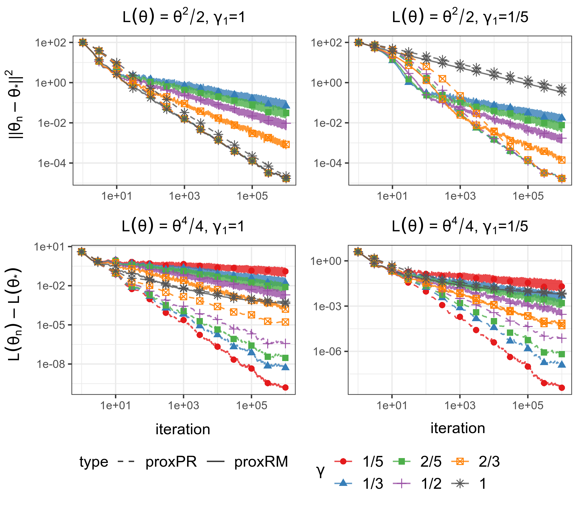
Figure 1: Error reduction for various learning rates.

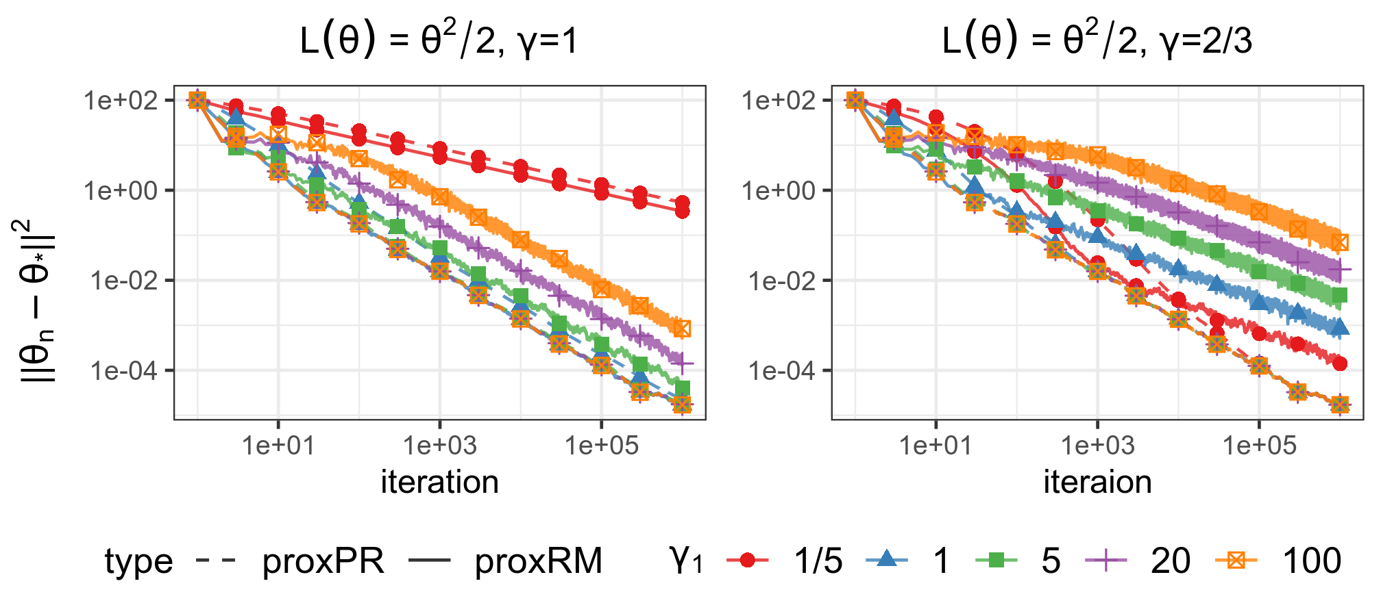
Figure 2: Error reduction for various values of initial step size.

Following Bach & Moulines (2011), we examined the convergence behavior of proxRM and proxPR using two univariate functions: $L(\theta)=\frac{1}{2}\theta^{2}$ (strongly convex) and $L(\theta)=\frac{1}{4}\theta^{4}$ (non-strongly convex); the sample functions were chosen $\ell(Z,\theta)=\frac{1}{2}\theta^{2}+Z\theta$ and $\ell(Z,\theta)=\frac{1}{4}\theta^{4}+Z\theta$, where $Z\sim N(0,4^{2})$. We fixed the initial point $\theta_{0}=10$ for the quadratic and $\theta_{0}=2$ for the quartic function, and observed 100 independent runs of $n=10^{6}$ ISGD iterations for initial step size $\gamma_{1}\in\{1/5,1,5,20,100\}$ and exponent $\gamma\in\{1/5,1/3,2/5,1/2,2/3,1\}$.

Figs. 1 and 2 plot the squared estimation ($\left\lVert\theta_{n}-\theta_{\star}\right\rVert^{2}$) or optimization ($L(\theta_{n})-L(\theta_{\star}$)) error averaged over all replications for each iteration. The trend generally aligns with the results in Sects. 4 and 5. First, several instances of proxPR showed slower reduction than proxRM in the early stage of the iteration, as expected by the theory. For the strongly convex case, the error reduction was proportional to $\gamma$ in proxRM and at the same fastest convergence rate in proxPR for all values except for $\gamma=1$, for which too small an initial step size showed a noticeable slowdown. For a given $\gamma$, the rate was proportional to $\gamma_{1}$ in proxRM, ending up with parallel lines in Fig. 2; in proxPR, the rate was independent of $\gamma$ and $\gamma_{1}$. Note that an initial step size as large as $100$ was allowed, with no explosion, confirming the stability of ISGD over SGD. For the non-strongly convex case, $\gamma=1$ was the fastest among proxRM if $\gamma_{1}$ was not too small but became the slowest among proxPR, for which slower decays led to faster convergence.

6.2 Interval estimation and inference

Table 2: Statistical inference for linear regression model parameters.

			ProxRM				ProxPR
$\Sigma$	$\gamma$	$p$	cover	MSE	lenCI	covdiff	cover	MSE	lenCI	covdiff
Identity	0.6	5	95.92	4.991e-3	0.285	5.817e-4	95.00	1.177e-5	0.013	1.299e-6
		20	97.54	4.424e-3	0.298	1.640e-3	95.01	1.270e-5	0.014	2.657e-6
		100	99.59	3.348e-3	0.334	4.180e-3	95.11	1.611e-5	0.016	7.309e-6
		200	99.97	2.511e-3	0.352	5.783e-3	95.05	1.782e-5	0.017	1.129e-5
	1	5	94.56	5.278e-5	0.028	3.436e-6	94.52	1.170e-5	0.013	1.344e-6
		20	95.14	5.245e-5	0.028	1.050e-5	94.70	1.151e-5	0.013	2.361e-6
		100	95.33	5.260e-5	0.029	2.353e-5	94.39	1.184e-5	0.013	5.456e-6
		200	95.48	5.197e-5	0.029	3.299e-5	94.44	1.192e-5	0.013	7.547e-6
Toeplitz	0.6	5	95.88	4.890e-3	0.285	6.979e-4	94.96	1.766e-5	0.017	2.037e-6
		20	97.40	4.439e-3	0.298	1.617e-3	94.96	2.082e-5	0.018	4.247e-6
		100	99.61	3.347e-3	0.334	4.185e-3	94.99	2.679e-5	0.020	1.194e-5
		200	99.96	2.525e-3	0.352	5.779e-3	95.19	2.959e-5	0.021	1.894e-5
	1	5	94.92	5.486e-5	0.029	4.976e-6	94.32	1.809e-5	0.016	1.874e-6
		20	95.05	5.518e-5	0.029	1.066e-5	93.95	1.985e-5	0.017	4.767e-6
		100	94.96	5.520e-5	0.029	2.487e-5	93.61	2.067e-5	0.017	9.691e-6
		200	95.47	5.396e-5	0.029	3.424e-5	93.88	2.083e-5	0.017	1.337e-5
EquiCorr	0.6	5	95.64	4.968e-3	0.285	6.030e-4	94.68	1.306e-5	0.014	1.490e-6
		20	97.42	4.454e-3	0.298	1.604e-3	94.90	1.532e-5	0.015	3.125e-6
		100	99.60	3.394e-3	0.334	4.159e-3	95.20	1.985e-5	0.018	8.990e-6
		200	99.95	2.583e-3	0.353	5.773e-3	95.13	2.228e-5	0.019	1.412e-5
	1	5	94.72	5.307e-5	0.029	3.199e-6	94.00	1.307e-5	0.014	1.518e-6
		20	95.15	5.326e-5	0.029	1.058e-5	94.49	1.403e-5	0.014	2.853e-6
		100	95.19	5.337e-5	0.029	2.391e-5	94.25	1.480e-5	0.015	6.827e-6
		200	95.45	5.267e-5	0.029	3.334e-5	94.36	1.497e-5	0.015	9.483e-6

Table 3: Statistical inference for quantile estimation.

Method	$\gamma$	$\mu$	cover	MSE	lenCI	covdiff
ProxRM	0.6	1e-3	95.20	1.339e-3	0.148	1.185e-4
		1e-2	95.60	1.315e-3	0.146	9.965e-5
		1e-1	95.40	1.191e-3	0.140	8.716e-5
	1	1e-3	96.60	4.933e-5	0.028	1.689e-6
		1e-2	96.00	4.887e-5	0.028	1.021e-6
		1e-1	91.40	5.769e-5	0.027	6.967e-7
ProxPR	0.6	1e-3	73.80	2.626e-5	0.016	4.363e-6
		1e-2	73.40	2.587e-5	0.015	3.262e-6
		1e-1	96.40	1.266e-5	0.015	2.755e-6
	1	1e-3	94.60	1.603e-5	0.016	1.246e-6
		1e-2	95.60	1.589e-5	0.015	5.692e-7
		1e-1	87.40	2.872e-5	0.015	5.506e-7

To evaluate the performance of the plug-in estimators of the asymptotic covariance matrices (Theorem 4.4 and Corollary 4.1), we conducted statistical inference on model parameters in linear regression and quantile estimation models using ISGD; see Chen et al. (2020); Toulis et al. (2021). Based on the observations on proxPR in the previous subsection, we discarded the first tenth of the iterations when calculating $\tilde{H}_{n},\hat{I}_{n}$, and $\bar{\theta}_{n}$. Then, we gathered the average rate of the nominal 95% confidence interval (13), (15) covering $\theta_{*}$ for each coordinate (“cover”), mean squared error from $\theta_{*}$ (“MSE”), and the length of the 95% confidence interval (“lenCI”) from $B=500$ independent replications. We also compared the plug-in estimator of each run with the multi-run estimator (11) using the Frobenius norm (normalized by dimension $p$); its average is reported (“covdiff”).

Linear regression. We generated $Z_{n}=(y_{n},\mathbf{x}_{n})$ where $y_{n}=\mathbf{x}_{n}^{T}\theta_{*}+\epsilon_{n}$, $\mathbb{R}^{p}\ni\mathbf{x}_{n}\sim N(0,\Sigma)$, and $\epsilon_{n}\sim N(0,1)$, for $\ell(Z_{n},\theta)=\frac{1}{2}(y_{n}-\mathbf{x}_{n}^{T}\theta)^{2}$. Three different covariance structures were considered: identity ($\Sigma=I_{p}$), Toeplitz ($\Sigma_{ij}=(0.5)^{|i-j|}$), and equicorrelation ($\Sigma_{ij}=0.2$ for $i\neq j$, $\Sigma_{ii}=1$). We fixed $\theta_{\star}=(1,\dotsc,1)^{T}$ and ran $n=10^{5}$ iterations of ISGD for $\gamma\in\{0.6,1.0\}$, $p\in\{5,20,100,200\}$ with $\theta_{0}=0$ for each type of $\Sigma$. Table 3 collects the results. The coverage rates generally observed the nominal level, with proxRM showing a slightly better coverage, possibly because proxPR exhibited shorter confidence intervals.

Quantile estimation. Since the sample function for quantile estimation introduced in Sect. 1 is nondifferentiable, we instead used a smoothed version in which the $\max(0,\cdot)$ part is replaced by a quadratic function $(4\mu)^{-1}(x+\mu)^{2}$ on $[-\mu,\mu]$. The smoothing parameter $\mu$ makes $\nabla\ell(Z,\theta)$ $(2\mu)^{-1}$-Lipschitz and introduces a bias. We nevertheless set $\theta_{\star}$ to be the 99%-ile of the standard normal and let $Z\sim N(0,1)$. The $n=10^{6}$ iterations were started with $\theta_{0}=0$ for each replication, where $\gamma\in\{0.6,1\}$ and $\mu\in\{10^{-1},10^{-2},10^{-3}\}$; we used $\gamma_{1}=250$ when $\gamma=1$ and $\gamma_{1}=30$ when $\gamma=0.6$. Table 3 summarizes the results. While proxPR exhibits smaller MSE and covdiff, the coverage rate of proxRM was close to 95% and there are few cases that proxPR deteriorates. This result may be misleading since the actual minimizer of $L$ is not $\theta_{\star}$ here, and the length of the confidence interval is smaller for proxPR. On the other hand, if the genuine goal is to find the quantile, the better coverage of (biased) proxRM might be a blessing.

7 Conclusion

In both point estimation of the model parameter for the strongly convex case and optimization of non-strongly convex functionals, the behavior of implicit SGD as revealed by our non-asymptotic analysis, either proxRM or proxPR, resembles the explicit SGD when the gradient is uniformly bounded a.s. on a bounded domain (Bach & Moulines, 2011, Theorems 2, 5, 7), which replaces Assumption(s) A4 (and, with strong convexity, A2). Thus ISGD effectively imposes the latter condition without requiring it, operating under weaker assumptions on the gradient map.

Like its explicit counterpart, our analysis (and experiments) states that averaging brings to ISGD robustness to the initial step size and lack of strong convexity. On the other hand, averaged ISGD (proxPR) may suffer from slow progress in the early phase of iterations. Burn-in is a viable option. It is interesting to note that the plug-in estimators of the asymptotic covariance matrices of proxRM and proxPR, indispensable for valid statistical inference on the model parameter, does not benefit from averaging. Since this paper appears to be the first to propose estimators based only on a single run, investigation of more statistically efficient estimators as well as online ones as in SGD (Chen et al., 2020) will make a promising avenue of future research.

Appendix A Proofs of main results

A.1 Preliminary

In this section, we collect known facts useful for the subsequent proofs.

Proposition A.1 (Bach & Moulines (2011), p. 17).

$$\left\lVert a+b\right\rVert^{k}\leq 2^{k-1}(\left\lVert a\right\rVert^{k}+\left\lVert b\right\rVert^{k}),\quad k=1,2,3,4.$$

Proposition A.2.

$$\gamma_{n}\leq\gamma_{n-1} \leq 2\gamma_{n},\quad n\geq 2;$$

$$\gamma_{n}^{1/2}-\gamma_{n+1}^{1/2} \geq\frac{\gamma_{1}^{1/2}}{4n^{\gamma/2}},\quad n\geq 3.$$

Proposition A.3.

Let $\phi_{\gamma}(n)=(n^{1-\gamma}-1)/(1-\gamma)$ if $\gamma>0$ and $\gamma\neq 1$, and $\phi_{\gamma}(n)=\log n$ if $\gamma=1$. Then,

$$\sum_{k=1}^{n}\frac{1}{k^{\gamma}}\leq 1+\phi_{\gamma}(n)\leq\begin{cases}\textstyle\frac{n^{1-\gamma}}{1-\gamma},&\gamma\in(0,1),\\ 1+\log n,&\gamma=1,\\ \zeta(\gamma):=\sum_{k=1}^{\infty}\frac{1}{k^{\gamma}}<\infty,&\gamma>1\end{cases}$$

and

$$\frac{1}{2}[\phi_{\gamma}(n)-\phi_{\gamma}(m)]\leq\sum_{k=m+1}^{n}\frac{1}{k^{\gamma}}\leq\phi_{\gamma}(n)-\phi_{\gamma}(m),\quad n>m\geq 1.$$

The last inequality is from Bach & Moulines (2011, p. 13).

A.2 Proof of Proposition 3.1

Proposition 3.1 can be proved by combining the following intermediate result and Lemma 3.1.

Lemma A.1 (Theorem 3.3 and Corollary 3.3 of Asi & Duchi (2019)).

In addition to Assumptions A1, A2, and A4, also assume that a minimizer $\theta_{\star}$ of $L$ exists (not necessarily unique). Then, the iterates from the ISGD update (3) with learning rate sequence (R) satisfies

$$\mathop{\mathbf{E}\,\!}\nolimits[\left\lVert\theta_{n}-\theta_{\star}\right\rVert^{2}|\mathcal{F}_{n-1}] \leq\left\lVert\theta_{n-1}-\theta_{\star}\right\rVert^{2}+\sigma^{2}\gamma_{n}^{2},\quad\gamma\in(0,1],$$

$$\mathop{\mathbf{E}\,\!}\nolimits\left\lVert\theta_{n}-\theta_{\star}\right\rVert^{2} \leq\left\lVert\theta_{0}-\theta_{\star}\right\rVert^{2}+\sigma^{2}\sum_{k=1}^{\infty}\gamma_{k}^{2}=r^{2}<\infty,\quad\gamma\in(1/2,1].$$

for all $n=1,2,\dotsc$.

Proof of Proposition 3.1.

Note that

$$\theta_{n} =\theta_{n-1}-\gamma_{n}\nabla\ell(Z_{n},\theta_{n})$$

$$=[\theta_{n-1}-\gamma_{n}\nabla\ell(Z_{n},\theta_{n-1})]+[\gamma_{n}\nabla\ell(Z_{n},\theta_{n-1})-\gamma_{n}\nabla\ell(Z_{n},\theta_{n})].$$

Thus $R_{n}=\gamma_{n}[\nabla\ell(Z_{n},\theta_{n-1})-\nabla\ell(Z_{n},\theta_{n})]$. Then,

$$\begin{split}\|R_{n}\|&=\gamma_{n}\|\nabla\ell(Z_{n},\theta_{n-1})-\nabla\ell(Z_{n},\theta_{n})]\|\\ &\leq\gamma_{n}\beta(Z_{n})\|\theta_{n-1}-\theta_{n}\|\leq\gamma_{n}^{2}\beta(Z_{n})\|\nabla\ell(Z_{n},\theta_{n-1})\|,\end{split}$$ (A.1)

where the first inequality is due to Assumption A2, and the second due to Lemma 3.1.

We show the bounds on $\left\lVert R_{n}\right\rVert$. First, observe from the triangular inequality and Assumption A2 that

$$\left\lVert\nabla\ell(Z_{n},\theta_{n-1})\right\rVert\leq\beta(Z_{n})\left\lVert\theta_{n-1}-\theta_{\star}\right\rVert+\left\lVert\nabla\ell(Z_{n},\theta_{\star})\right\rVert.$$ (A.2)

Then,

$$\begin{split}\mathop{\mathbf{E}\,\!}\nolimits{[\left\lVert R_{n}\right\rVert|\mathcal{F}_{n-1}]}&\leq\gamma_{n}^{2}\mathop{\mathbf{E}\,\!}\nolimits{[\beta^{2}(Z_{n})]}\left\lVert\theta_{n-1}-\theta_{\star}\right\rVert\\ &\quad+(1/2)\gamma_{n}^{2}\mathop{\mathbf{E}\,\!}\nolimits{[\beta^{2}(Z_{n})]}+(1/2)\gamma_{n}^{2}\mathop{\mathbf{E}\,\!}\nolimits{\left\lVert\nabla\ell(Z_{n},\theta_{\star})\right\rVert^{2}}\\ &\leq\gamma_{n}^{2}\beta_{0}^{2}\left\lVert\theta_{n-1}-\theta_{\star}\right\rVert+(1/2)\gamma_{n}^{2}\beta_{0}^{2}+(1/2)\gamma_{n}^{2}\sigma^{2}\end{split}$$ (A.3)

using $2ab\leq a^{2}+b^{2}$ and Assumption A2. Therefore for $\gamma\in(1/2,1]$ with which $r<\infty$,

$$\mathop{\mathbf{E}\,\!}\nolimits{\left\lVert R_{n}\right\rVert}\leq\gamma_{n}^{2}\beta_{0}^{2}\mathop{\mathbf{E}\,\!}\nolimits{\left\lVert\theta_{n-1}-\theta_{\star}\right\rVert}+(1/2)\gamma_{n}^{2}(\beta_{0}^{2}+\sigma^{2})\leq\gamma_{n}^{2}[\beta_{0}^{2}(r+1/2)+\sigma^{2}/2].$$

The last inequality is due to Lemma A.1 and Jensen’s inequality.

To establish bounds on $\left\lVert R_{n}\right\rVert^{2}$, from inequality (A.2),

$$\left\lVert\nabla\ell(Z_{n},\theta_{n-1})\right\rVert^{2} \leq 2\beta^{2}(Z_{n})\left\lVert\theta_{n-1}-\theta_{\star}\right\rVert^{2}+2\left\lVert\nabla\ell(Z_{n},\theta_{\star})\right\rVert^{2}$$

using $(a+b)^{2}\leq 2a^{2}+2b^{2}$. So

$$\mathop{\mathbf{E}\,\!}\nolimits{[\left\lVert\nabla\ell(Z_{n},\theta_{n-1})\right\rVert^{2}|\mathcal{F}_{n-1}]}\leq 2\beta_{0}^{2}\left\lVert\theta_{n-1}-\theta_{\star}\right\rVert^{2}+2\sigma^{2}$$ (A.4)

from Assumption A4. Then, by the definition of $R_{n}$,

$$\mathop{\mathbf{E}\,\!}\nolimits{[\left\lVert R_{n}\right\rVert^{2}|\mathcal{F}_{n-1}]} =\gamma_{n}^{2}\mathop{\mathbf{E}\,\!}\nolimits{[\left\lVert\nabla\ell(Z_{n},\theta_{n})-\nabla\ell(Z_{n},\theta_{n-1})\right\rVert^{2}|\mathcal{F}_{n-1}]}$$

$$=\gamma_{n}^{2}\mathop{\mathbf{E}\,\!}\nolimits{[\left\lVert\nabla\ell(Z_{n},\theta_{n})\right\rVert^{2}|\mathcal{F}_{n-1}]}-2\gamma_{n}^{2}\mathop{\mathbf{E}\,\!}\nolimits{[\nabla\ell(Z_{n},\theta_{n})^{T}\nabla\ell(Z_{n},\theta_{n-1})|\mathcal{F}_{n-1}]}$$

$$\quad+\gamma_{n}^{2}\mathop{\mathbf{E}\,\!}\nolimits{[\left\lVert\nabla\ell(Z_{n},\theta_{n-1})\right\rVert^{2}|\mathcal{F}_{n-1}]}$$

$$\leq 4\gamma_{n}^{2}\mathop{\mathbf{E}\,\!}\nolimits{[\left\lVert\nabla\ell(Z_{n},\theta_{n-1})\right\rVert^{2}|\mathcal{F}_{n-1}]}\leq 8\gamma_{n}^{2}\beta_{0}^{2}\left\lVert\theta_{n-1}-\theta_{\star}\right\rVert^{2}+8\gamma_{n}^{2}\sigma^{2}$$

using the Cauchy-Schwarz inequality and Lemma 3.1. Then, for $\gamma\in(1/2,1]$,

$$\mathop{\mathbf{E}\,\!}\nolimits{\left\lVert R_{n}\right\rVert^{2}}\leq 8\gamma_{n}^{2}\beta_{0}^{2}\mathop{\mathbf{E}\,\!}\nolimits{\left\lVert\theta_{n-1}-\theta_{\star}\right\rVert^{2}}+8\gamma_{n}^{4}\sigma^{2}\leq 8\gamma_{n}^{2}(\beta_{0}^{2}r^{2}+\sigma^{2})$$ (A.5)

from Lemma A.1. ∎

A.3 Proof of Theorem 4.1

We enhance the result by Toulis & Airoldi (2017a, Lemma 2.2 in the Supplement):

Lemma A.2.

Consider positive sequences $a_{n}$ such that $\sum_{k=1}^{\infty}a_{k}=A<\infty$, $b_{n}\downarrow 0$, and $c_{n}\downarrow 0$, and there is $n^{\prime}$ such that $c_{n}/b_{n}<1$ for all $n>n^{\prime}$. Let

$$\delta_{n}=\frac{1}{a_{n}}\left(\frac{a_{n-1}}{b_{n-1}}-\frac{a_{n}}{b_{n}}\right),\quad\zeta_{n}=\frac{c_{n}}{b_{n-1}}\frac{a_{n-1}}{a_{n}}$$

and suppose $\delta_{n}\downarrow\delta\geq 0$ and $\zeta_{n}\downarrow 0$. Then, for a nonnegative sequence $y_{n}$ such that

$$y_{n}\leq\frac{1+c_{n}}{1+(1+\delta)b_{n}}y_{n-1}+a_{n},$$ (A.6)

there holds

$$y_{n}\leq K_{0}\frac{a_{n}}{b_{n}}+Q_{1}^{n}y_{0}+Q_{n_{0}+1}^{n}[(1+c_{1})^{n_{0}}A+B]$$ (A.7)

for every $n=1,2,\dotsc$, where $n_{0}$ is an integer such that $\delta_{n}+\zeta_{n}<1+\delta$ and $c_{n}<(1+\delta)b_{n}$ for all $n\geq n_{0}$, $K_{0}=[1+(1+\delta)b_{1}]/(1+\delta-\delta_{n_{0}}-\zeta_{n_{0}})$, $B=K_{0}a_{n_{0}}/b_{n_{0}}$, and $Q_{i}^{n}=\prod_{j=i}^{n}(1+c_{j})/(1+(1+\delta)b_{j})$ if $n\geq i$ and $Q_{i}^{n}=1$ otherwise.

Proof.

See Sect. B. ∎

Corollary A.1.

Let $\alpha>\beta>\gamma$ where $\alpha>1$ and $\gamma\in(0,1]$. Consider a nonnegative sequence $\{y_{n}\}$ such that

$$y_{n}\leq(1-\eta n^{-\gamma}+\nu n^{-\beta})y_{n-1}+a_{1}n^{-\alpha}$$ (A.8)

with $\eta>0$, $\nu\geq 0$, and $a_{1}\geq 0$. If $\gamma=1$, assume that $\eta>\alpha-\gamma$. Then, there holds

$$y_{n}\leq K_{1}n^{-(\alpha-\gamma)}+K_{2}(n)\exp\left(-\textstyle\frac{1}{2}\log(1+\eta)\phi_{\gamma}(n)\right)(y_{0}+D_{n_{0}}),$$ (A.9)

where

$$\phi_{\gamma}(n)=\begin{cases}(n^{1-\gamma}-1)/(1-\gamma),&\gamma\in(0,1),\\ \log n,&\gamma=1,\end{cases}\quad\text{and}\quad\delta=\begin{cases}0,&\gamma\in(0,1),\\ 1/(\frac{\eta}{\alpha-\gamma}-1),&\gamma=1.\end{cases}$$

and

$$K_{1} =K_{0}\frac{a_{1}(1+\delta)}{\eta},$$ (A.10a)

$$K_{2}(n) =\begin{cases}\exp\left(\nu(1+\eta)\sum_{k=1}^{\infty}k^{-\beta}\right)<\infty,&\beta>1,\\ \exp\big{(}\nu(1+\eta)\phi_{\beta}(n)\big{)},&\beta\leq 1,\end{cases}$$ (A.10b)

$$D_{n_{0}} =(1+\eta)^{n_{0}}\big{(}[1+\nu(1+\eta)]^{n_{0}}A+B\big{)},$$ (A.10c)

$$A =a_{1}\sum_{k=1}^{\infty}k^{-\alpha}<\infty,\quad B=K_{0}(1+\delta)\eta^{-1}a_{1}n_{0}^{-(\alpha-\gamma)}.$$ (A.10d)

The $n_{0}$ is an integer such that

$$n^{\gamma}\big{(}[n/(n-1)]^{\alpha-\gamma}-1\big{)}+\nu(1+\eta)[n/(n-1)]^{\alpha-\gamma}n^{-\gamma} <\eta$$ (A.11a)

$$\nu(1+\eta)n^{-\gamma} <\eta$$ (A.11b)

for all $n\geq n_{0}$. The constant $K_{0}$ is given by

$$K_{0}=\frac{(1+\eta)/(1+\delta)}{1-\left(\frac{n_{0}^{-\gamma}}{\eta}([\frac{n_{0}}{n_{0}-1}]^{\alpha-\gamma}-1)+\frac{\nu(1+\eta)}{\eta}n_{0}^{-(\beta-\gamma)}[\frac{n_{0}}{n_{0}-1}]^{\alpha-\gamma}\right)}.$$

In particular, if $\nu=0$, then $K_{2}(n)\equiv 1$.

Proof.

See Sect. B. ∎

Proof of Theorem 4.1.

From Proposition 3.1, one can obtain

$$\mathop{\mathbf{E}\,\!}\nolimits\left\lVert\theta_{n}-\theta_{\star}\right\rVert^{2}= \mathop{\mathbf{E}\,\!}\nolimits\left\lVert\theta_{n-1}-\theta_{\star}\right\rVert^{2}$$ (A.12a)

$$-2\gamma_{n}\mathop{\mathbf{E}\,\!}\nolimits[(\theta_{n-1}-\theta_{\star})^{T}\nabla\ell(Z_{n},\theta_{n-1})]$$ (A.12b)

$$+\gamma_{n}^{2}\mathop{\mathbf{E}\,\!}\nolimits\left\lVert\nabla\ell(Z_{n},\theta_{n-1})\right\rVert^{2}$$ (A.12c)

$$+2\mathop{\mathbf{E}\,\!}\nolimits[(\theta_{n-1}-\theta_{\star})^{T}R_{n}]$$ (A.12d)

$$-2\mathop{\mathbf{E}\,\!}\nolimits[R_{n}^{T}\nabla\ell(Z_{n},\theta_{n-1})]$$ (A.12e)

$$+\mathop{\mathbf{E}\,\!}\nolimits\left\lVert R_{n}\right\rVert^{2}.$$ (A.12f)

The second term (A.12b) is upper bounded as follows.

$$\begin{split}-2\gamma_{n}&\mathop{\mathbf{E}\,\!}\nolimits[(\theta_{n-1}-\theta_{\star})^{T}\nabla\ell(Z_{n},\theta_{n-1})]\\ &=-2\gamma_{n}\mathop{\mathbf{E}\,\!}\nolimits\mathop{\mathbf{E}\,\!}\nolimits[(\theta_{n-1}-\theta_{\star})^{T}\nabla\ell(Z_{n},\theta_{n-1})|\mathcal{F}_{n-1}]\\ &=-2\gamma_{n}\mathop{\mathbf{E}\,\!}\nolimits[(\theta_{n-1}-\theta_{\star})^{T}\mathop{\mathbf{E}\,\!}\nolimits[\nabla\ell(Z_{n},\theta_{n-1})|\mathcal{F}_{n-1}]]\\ &=-2\gamma_{n}\mathop{\mathbf{E}\,\!}\nolimits[(\theta_{n-1}-\theta_{\star})^{T}\nabla L(\theta_{n-1})]\\ &=-2\gamma_{n}\mathop{\mathbf{E}\,\!}\nolimits[(\theta_{n-1}-\theta_{\star})^{T}(\nabla L(\theta_{n-1})-\nabla L(\theta_{\star}))]\\ &\leq-2\gamma_{n}\lambda\mathop{\mathbf{E}\,\!}\nolimits\left\lVert\theta_{n-1}-\theta_{\star}\right\rVert^{2}.\end{split}$$ (A.13)

The last inequality is due to Assumption A3 and Remark 2.2; the penultimate inequality is due to $\nabla L(\theta_{\star})=0$.

In order to bound the third term (A.12c), from inequality (A.4) in the proof of Proposition 3.1,

$$\gamma_{n}^{2}\mathop{\mathbf{E}\,\!}\nolimits\left\lVert\nabla\ell(Z_{n},\theta_{n-1})\right\rVert^{2} \leq 2\gamma_{n}^{2}\beta_{0}^{2}\mathop{\mathbf{E}\,\!}\nolimits{\left\lVert\theta_{n-1}-\theta_{\star}\right\rVert^{2}}+2\gamma_{n}^{2}\sigma^{2}$$

$$\leq 2\gamma_{n}^{2}(\beta_{0}^{2}r^{2}+\sigma^{2}).$$

The last line follows from Lemma A.1.

Also for the term (A.12d), from the Cauchy-Schwarz and inequality (6a) in Proposition 3.1 we have

$$\mathop{\mathbf{E}\,\!}\nolimits{[(\theta_{n-1}-\theta_{\star})^{T}R_{n}|\mathcal{F}_{n-1}]} \leq\mathop{\mathbf{E}\,\!}\nolimits{[\left\lVert\theta_{n-1}-\theta_{\star}\right\rVert\left\lVert R_{n}\right\rVert|\mathcal{F}_{n-1}]}$$

$$=\left\lVert\theta_{n-1}-\theta_{\star}\right\rVert\mathop{\mathbf{E}\,\!}\nolimits{[\left\lVert R_{n}\right\rVert|\mathcal{F}_{n-1}]}$$

$$\leq\gamma_{n}^{2}\beta_{0}^{2}\left\lVert\theta_{n-1}-\theta_{\star}\right\rVert^{2}+\gamma_{n}^{2}(\beta_{0}^{2}+\sigma^{2})\left\lVert\theta_{n-1}-\theta_{\star}\right\rVert.$$

Thus

$$2\mathop{\mathbf{E}\,\!}\nolimits{[(\theta_{n-1}-\theta_{\star})^{T}R_{n}]}\leq 2\gamma_{n}^{2}[\beta_{0}^{2}r^{2}+(\beta_{0}^{2}+\sigma^{2})r]$$

using Lemma A.1 and Jensen’s inequality.

For the term (A.12e), we obtain

$$- \mathop{\mathbf{E}\,\!}\nolimits{[R_{n}^{T}\nabla\ell(Z_{n},\theta_{n-1})|\mathcal{F}_{n-1}]}=-\mathop{\mathbf{E}\,\!}\nolimits{[\gamma_{n}[\nabla\ell(Z_{n},\theta_{n-1})-\nabla\ell(Z_{n},\theta_{n})]^{T}\nabla\ell(Z_{n},\theta_{n-1})|\mathcal{F}_{n-1}]}$$

$$\quad=-\gamma_{n}\mathop{\mathbf{E}\,\!}\nolimits{[\left\lVert\nabla\ell(Z_{n},\theta_{n-1})\right\rVert^{2}|\mathcal{F}_{n-1}]}+\gamma_{n}\mathop{\mathbf{E}\,\!}\nolimits{\nabla\ell(Z_{n},\theta_{n})^{T}\nabla\ell(Z_{n},\theta_{n-1})|\mathcal{F}_{n-1}]}$$

$$\quad\leq-\gamma_{n}\mathop{\mathbf{E}\,\!}\nolimits{[\left\lVert\nabla\ell(Z_{n},\theta_{n-1})\right\rVert^{2}|\mathcal{F}_{n-1}]}+\gamma_{n}\mathop{\mathbf{E}\,\!}\nolimits{\left\lVert\nabla\ell(Z_{n},\theta_{n})\right\rVert\left\lVert\nabla\ell(Z_{n},\theta_{n-1})\right\rVert|\mathcal{F}_{n-1}]}$$

$$\quad\leq-\gamma_{n}\mathop{\mathbf{E}\,\!}\nolimits{[\left\lVert\nabla\ell(Z_{n},\theta_{n-1})\right\rVert^{2}|\mathcal{F}_{n-1}]}+\gamma_{n}\mathop{\mathbf{E}\,\!}\nolimits{[\left\lVert\nabla\ell(Z_{n},\theta_{n-1})\right\rVert^{2}|\mathcal{F}_{n-1}]}$$

$$\quad=0,$$

where the last inequality is due to Lemma 3.1. Thus we have $-2\mathop{\mathbf{E}\,\!}\nolimits{[R_{n}^{T}\nabla\ell(Z_{n},\theta_{n-1})]}\leq 0$.

The final term (A.12) is bounded by inequality (6d) in Proposition 3.1.

Combining these results yields

$$\mathop{\mathbf{E}\,\!}\nolimits{\left\lVert\theta_{n}-\theta_{\star}\right\rVert^{2}} \leq(1-2\lambda\gamma_{n})\mathop{\mathbf{E}\,\!}\nolimits\left\lVert\theta_{n-1}-\theta_{\star}\right\rVert^{2}+2[6\beta_{0}^{2}r^{2}+5\sigma^{2}+(\beta_{0}^{2}+\sigma^{2})r]\gamma_{n}^{2}.$$

Now we can apply Corollary A.1 by setting $y_{n}=\mathop{\mathbf{E}\,\!}\nolimits{\left\lVert\theta_{n}-\theta_{\star}\right\rVert^{2}}$, $\alpha=2\gamma$, $a_{1}=2[6\beta_{0}^{2}r^{2}+5\sigma^{2}+(\beta_{0}^{2}+\sigma^{2})r]$, $\gamma_{1}^{2}$, $\eta=2\lambda\gamma_{1}>0$, and $\nu=0$. This proves the claim.

Below we put the explicit values of the constants:

$$\delta =\begin{cases}0,&\gamma\in(1/2,1),\\ 1/(2\lambda\gamma_{1}-1),&\gamma=1,\end{cases}$$

$$K_{0} =\frac{1/(1+\delta)+\gamma_{1}}{1-\frac{n_{0}^{\gamma}}{2\lambda\gamma_{1}}([\frac{n_{0}}{n_{0}-1}]^{\gamma}-1)},$$

$$K_{1} =K_{0}\frac{2[6\beta_{0}^{2}r^{2}+5\sigma^{2}+(\beta_{0}^{2}+\sigma^{2})r]\gamma_{1}(1+\delta)}{2\lambda},$$

$$K_{2}(n) \equiv 1,$$

$$D_{n_{0}} =(1+2\lambda\gamma_{1})^{n_{0}}(A+B),$$

$$A =2[6\beta_{0}^{2}r^{2}+5\sigma^{2}+(\beta_{0}^{2}+\sigma^{2})r]\gamma_{1}^{2}\sum_{k=1}^{\infty}k^{-2\gamma}<\infty,$$

$$B =2K_{0}[6\beta_{0}^{2}r^{2}+5\sigma^{2}+(\beta_{0}^{2}+\sigma^{2})r]\gamma_{1}n_{0}^{-\gamma}.$$

∎

A.4 Proof of Theorem 4.2

Proof of Theorem 4.2.

Suppose the following holds.

$$\mathop{\mathbf{E}\,\!}\nolimits{[\nabla\ell(Z_{n},\theta_{n})]}=\mathcal{H}(\theta_{\star})\mathop{\mathbf{E}\,\!}\nolimits{[\theta_{n}-\theta_{\star}]}+O(\gamma_{n}^{1/2}).$$ (A.14)

Taking expectations on the update equation $\theta_{n}=\theta_{n-1}-\gamma_{n}\nabla\ell(Z_{n},\theta_{n})$, equation (A.14) entails

$$\mathop{\mathbf{E}\,\!}\nolimits{[\theta_{n}-\theta_{\star}]}=\mathop{\mathbf{E}\,\!}\nolimits{[\theta_{n-1}-\theta_{\star}]}-\gamma_{n}\mathcal{H}(\theta_{\star})\mathop{\mathbf{E}\,\!}\nolimits{[\theta_{n}-\theta_{\star}]}+O(\gamma_{n}^{1/2}),$$

or

$$\mathop{\mathbf{E}\,\!}\nolimits{[\theta_{n}-\theta_{\star}]} =[I+\gamma_{n}\mathcal{H}(\theta_{\star})]^{-1}\mathop{\mathbf{E}\,\!}\nolimits{[\theta_{n-1}-\theta_{\star}]}+[I+\gamma_{n}\mathcal{H}(\theta_{\star})]^{-1}O(\gamma_{n}^{1/2}).$$

By recursively applying the above equation, we see

$$\mathop{\mathbf{E}\,\!}\nolimits{[\theta_{n}-\theta_{\star}]} =Q_{1}^{n}(\theta_{0}-\theta_{\star})+Q_{1}^{n}O(\sum_{k=1}^{n}\gamma_{k}^{1/2})=Q_{1}^{n}(\theta_{0}-\theta_{\star})+Q_{1}^{n}O(n^{1-\gamma/2}).$$

Note $\left\lVert Q_{1}^{n}\right\rVert=\left\lVert\prod_{i=1}^{n}[I+\gamma_{i}\mathcal{H}(\theta_{\star})]^{-1}\right\rVert\leq(\prod_{i=1}^{n}(1+\lambda\gamma_{i}))^{-1}$ where $\lambda\leq\lambda_{\min}(\mathcal{H}(\theta_{\star}))$. From inequality (B.5), $Q_{1}^{n}=O(\exp(-\kappa n^{1-\gamma}))$ if $\gamma\in(1/2,1)$ and $Q_{1}^{n}=O(n^{-\kappa})$ if $\gamma=1$, where $\kappa=\log(1+\lambda\gamma_{1})>0$. In either case, we have $Q_{1}^{n}O(n^{1-\gamma/2})=o(1)$ as desired (when $\gamma=1$, we are given $\gamma_{1}\geq(e^{2}-1)/\lambda$ with which $\kappa\geq 1$).

To see equation (A.14) holds, recall that the objective function $L$ is twice differentiable at $\theta_{\star}$. It follows that

$$\begin{split}\nabla\ell(Z_{n},\theta_{n})&=W_{n}+\mathcal{H}(\theta_{\star})(\theta_{n}-\theta_{\star})+o(\left\lVert\theta_{n}-\theta_{\star}\right\rVert),\\ &=W_{n}+\mathcal{H}(\theta_{\star})(\theta_{n}-\theta_{\star})+o(\gamma_{n}^{1/2}),\\ W_{n}&=\nabla\ell(Z_{n},\theta_{n})-\nabla L(\theta_{n}),\end{split}$$ (A.15)

From Proposition 3.1, we see $\nabla\ell(Z_{n},\theta_{n})=\nabla\ell(Z_{n},\theta_{n-1})-\gamma_{n}^{-1}R_{n}$ and $\mathop{\mathbf{E}\,\!}\nolimits[R_{n}]=O(\gamma_{n}^{2})$. In other words, $W_{n}=\nabla\ell(Z_{n},\theta_{n-1})-L(\theta_{n})-\gamma_{n}^{-1}R_{n}$ and

$$\mathop{\mathbf{E}\,\!}\nolimits[W_{n}]=\nabla L(\theta_{n-1})-\nabla L(\theta_{n})+O(\gamma_{n}).$$

The difference of the first two terms are bounded as follows.

$$\left\lVert\nabla L(\theta_{n})-\nabla L(\theta_{n-1})\right\rVert =\left\lVert\mathop{\mathbf{E}\,\!}\nolimits[\nabla\ell(Z,\theta_{n})-\nabla\ell(Z,\theta_{n-1})]\right\rVert$$

$$\leq\mathop{\mathbf{E}\,\!}\nolimits\left\lVert\nabla\ell(Z,\theta_{n})-\nabla\ell(Z,\theta_{n-1})\right\rVert\quad\text{(Jensen's inequality)}$$

$$\leq\mathop{\mathbf{E}\,\!}\nolimits{\left\lVert\nabla\ell(Z,\theta_{n})-\nabla\ell(Z,\theta_{\star})\right\rVert}+\mathop{\mathbf{E}\,\!}\nolimits{\left\lVert\nabla\ell(Z,\theta_{n-1})-\nabla\ell(Z,\theta_{\star})\right\rVert}$$

$$\leq\mathop{\mathbf{E}\,\!}\nolimits{[\beta(Z)\left\lVert\theta_{n}-\theta_{\star}\right\rVert]}+\mathop{\mathbf{E}\,\!}\nolimits{[\beta(Z)\left\lVert\theta_{n-1}-\theta_{\star}\right\rVert]}\quad\text{(Assumption \ref{enum:Lipschitz})}$$

$$\leq(\mathop{\mathbf{E}\,\!}\nolimits{[\beta^{2}(Z)]})^{1/2}(\mathop{\mathbf{E}\,\!}\nolimits{\left\lVert\theta_{n}-\theta_{\star}\right\rVert}^{2})^{1/2}$$

$$\quad+(\mathop{\mathbf{E}\,\!}\nolimits{[\beta^{2}(Z)]})^{1/2}(\mathop{\mathbf{E}\,\!}\nolimits{\left\lVert\theta_{n-1}-\theta_{\star}\right\rVert}^{2})^{1/2}\quad\text{(Cauchy-Schwarz)}$$

$$=O(\gamma_{n}^{1/2}),$$

where the last inequality is due to Assumption A2 and Theorem 4.1. Hence $\mathop{\mathbf{E}\,\!}\nolimits[W_{n}]=O(\gamma_{n}^{1/2})$. Finally, by taking expectations on both sides of equation (A.15), equation (A.14) follows. ∎

A.5 Proof of Theorem 4.3

The proof utilizes Fabian’s central limit theorem for stochastic approximation Fabian (1968, Theorem 2.2) to show the asymptotic normality (9).

Lemma A.3 (Fabian).

Let $U_{n}$, $V_{n}$, $T_{n}\in\mathbb{R}^{p}$ and $\Phi_{n}$, $\Gamma_{n}\in\mathbb{R}^{p\times p}$ satisfy the following equation

$$U_{n}=(I-n^{-\alpha}\Gamma_{n})U_{n-1}+n^{-(\alpha+\beta)/2}\Phi_{n}V_{n}+n^{-\alpha-\beta/2}T_{n}$$

for $\alpha\in(0,1]$ and $\beta\geq 0$, where $\Gamma_{n}\rightarrow\Gamma\succ 0$, $\Phi_{n}\rightarrow\Phi$, $T_{n}\rightarrow T$ or $\mathop{\mathbf{E}\,\!}\nolimits\left\lVert T_{n}-T\right\rVert\rightarrow 0$, $\mathop{\mathbf{E}\,\!}\nolimits[V_{n}|\mathcal{F}_{n-1}]=0$, $C>\left\lVert\mathop{\mathbf{E}\,\!}\nolimits[V_{n}V_{n}^{T}-\Sigma|\mathcal{F}_{n-1}\right\rVert]\rightarrow 0$ for some $C$ and $\mathcal{F}_{n}$ a non-decreasing sequence of $\sigma$-fields such that $\Gamma_{n}$, $\Phi_{n}$, and $V_{n}$ are $\mathcal{F}_{n}$-measurable. Suppose $\sigma^{2}_{j,r}=\mathop{\mathbf{E}\,\!}\nolimits[I_{\left\lVert V_{j}\right\rVert^{2}\geq rj^{\alpha}}\left\lVert V_{j}\right\rVert^{2}]$, and either $\lim_{j\rightarrow\infty}\sigma^{2}_{j,r}=0$ for every $r>0$ or $\alpha=1$ and $\lim_{n\rightarrow\infty}n^{-1}\sum_{j=1}^{n}\sigma^{2}_{j,r}=0$ for every $r>0$. Let $\beta_{+}=\beta$ if $\alpha=1$, $\beta_{+}=0$ if $\alpha\neq 1$ and assume $\Gamma\succ(\beta_{+}/2)I$. Then the asymptotic distribution of $n^{\beta/2}U_{n}$ is normal with mean $(\Gamma-(\beta_{+}/2)I)^{-1}T$ and covariance matrix $\mathcal{L}_{2\Gamma-\beta_{+}I}^{-1}(\Phi\Sigma\Phi^{T})$, where $\mathcal{L}_{P}:X\mapsto(1/2)(PX+XP)$ is the Lyapunov linear map.

If $P\succ 0$, the inverse linear map $\mathcal{L}_{P}^{-1}$ is well-defined; if furthermore $C\succ 0$, then $\mathcal{L}_{P}^{-1}(C)\succ 0$.

Proof of Theorem 4.3.

Using Proposition 3.1, the implicit update equation becomes

$$\begin{split}\theta_{n}&=\theta_{n-1}-\gamma_{n}\nabla\ell(Z_{n},\theta_{n})\\ &=\theta_{n-1}-\gamma_{n}\nabla\ell(Z_{n},\theta_{n-1})+R_{n}\\ &=\theta_{n-1}-\gamma_{n}[\nabla L(\theta_{n-1})+\nabla\ell(Z_{n},\theta_{n-1})-\nabla L(\theta_{n-1})]+O(\gamma_{n}^{2})\\ &=\theta_{n-1}-\gamma_{n}\nabla L(\theta_{n-1})+\gamma_{n}\varepsilon_{n}+O(\gamma_{n}^{2}),\end{split}$$ (A.16)

where $\varepsilon_{n}=\nabla L(\theta_{n-1})-\nabla\ell(Z_{n},\theta_{n-1})$. Since $L$ is twice differentiable at $\theta_{\star}$, we further have

$$\begin{split}\theta_{n}-\theta_{\star}&=\theta_{n-1}-\theta_{\star}-\gamma_{n}\mathcal{H}(\theta_{\star})(\theta_{n-1}-\theta_{\star})+\gamma_{n}o(\left\lVert\theta_{n-1}-\theta_{\star}\right\rVert)+\gamma_{n}\varepsilon_{n}+O(\gamma_{n}^{2})\\ &=\theta_{n-1}-\theta_{\star}-\gamma_{n}\mathcal{H}(\theta_{\star})(\theta_{n-1}-\theta_{\star})+\gamma_{n}o(\gamma_{n-1}^{1/2})+\gamma_{n}\varepsilon_{n}+O(\gamma_{n}^{2})\\ &=\theta_{n-1}-\theta_{\star}-\gamma_{n}\mathcal{H}(\theta_{\star})(\theta_{n-1}-\theta_{\star})+o(\gamma_{n}^{3/2})+\gamma_{n}\varepsilon_{n}+O(\gamma_{n}^{2})\\ &=[I-\gamma_{n}\mathcal{H}(\theta_{\star})](\theta_{n-1}-\theta_{\star})+\gamma_{n}\varepsilon_{n}+o(\gamma_{n}^{3/2}),\end{split}$$ (A.17)

where the second line is due to Theorem 4.1 and $\theta_{n-1}\to\theta_{\star}$ a.s. For the third line, recall that $\gamma_{n}=\gamma_{1}n^{-\gamma}$ (R).

In order to apply Lemma A.3, observe that $\mathop{\mathbf{E}\,\!}\nolimits[\varepsilon_{n}|\mathcal{F}_{n-1}]=0$ and

$$\mathop{\mathbf{E}\,\!}\nolimits[\varepsilon_{n}\varepsilon_{n}^{T}|\mathcal{F}_{n-1}] =\mathop{\mathbf{E}\,\!}\nolimits[(\nabla L(\theta_{n-1})-\nabla\ell(Z_{n},\theta_{n-1}))(\nabla L(\theta_{n-1})-\nabla\ell(Z_{n},\theta_{n-1}))^{T}|\mathcal{F}_{n-1}]$$

$$=\mathop{\mathbf{E}\,\!}\nolimits[(\nabla L(\theta_{n-1})-\nabla\ell(Z,\theta_{n-1}))(\nabla L(\theta_{n-1})-\nabla\ell(Z,\theta_{n-1}))^{T}]$$

$$=\mathcal{I}(\theta_{n-1})$$

since $\theta_{n-1}\in\mathcal{F}_{n-1}$. To meet the conditions for Lemma A.3, it suffices to show that $\mathcal{I}$ is continuous at $\theta_{\star}$. Consider a non-random convergent sequence $\{\vartheta_{n}\}$ such that $\vartheta_{n}\to\theta_{\star}$. Fix $\epsilon>0$. Then there exists $n_{0}$ such that for all $n\geq n_{0}$, $\left\lVert\vartheta_{n}-\theta_{\star}\right\rVert\leq\epsilon$. Then,

$$\left\lVert\nabla\ell(Z,\vartheta_{n})\nabla\ell(Z,\vartheta_{n})^{T}\right\rVert \leq\left\lVert\nabla\ell(Z,\vartheta_{n})\right\rVert^{2}$$

$$\leq 2\beta^{2}(Z)\left\lVert\vartheta_{n}-\vartheta_{\star}\right\rVert^{2}+2\left\lVert\nabla\ell(Z,\theta_{\star})\right\rVert^{2}$$

$$\leq 2\beta^{2}(Z)\epsilon^{2}+2\left\lVert\nabla\ell(Z,\theta_{\star})\right\rVert^{2}$$

for all $n\geq n_{0}$. The last line is integrable due to Assumptions A2 and A4. Therefore, by the dominated convergence theorem, $\mathcal{I}(\vartheta_{n})=\mathop{\mathbf{E}\,\!}\nolimits{[\nabla\ell(Z,\vartheta_{n})\nabla\ell(Z,\vartheta_{n})^{T}]}-\nabla L(\vartheta_{n})L(\vartheta_{n})^{T}<\infty$ and $\mathcal{I}(\vartheta_{n})\to\mathcal{I}(\theta_{\star})$ and $\mathcal{I}$ is continuous at $\theta_{\star}$.

Letting $U_{n}=\theta_{n}-\theta_{\star}$, $V_{n}=\varepsilon_{n}$, $T_{n}=o(1)$, $\Phi_{n}=\Phi=\gamma_{1}I$, $\Gamma_{n}=\Gamma=\gamma_{1}\mathcal{H}(\theta_{\star})$, $T=0$, $\Sigma=\mathcal{I}(\theta_{\star})$, and $\alpha=\beta=\gamma$ in Lemma A.3 results in the desired asymptotic normality. ∎

Remark A.1.

The approximation of ISGD to SGD in Proposition 3.1 is crucial since otherwise $\varepsilon_{n}$ would equal to $\nabla L(\theta_{n})-\nabla\ell(Z_{n},\theta_{n})$. Since $\theta_{n}\notin\mathcal{F}_{n-1}$, we do not have $\mathop{\mathbf{E}\,\!}\nolimits[\varepsilon_{n}|\mathcal{F}_{n-1}]=0$. That is, $\varepsilon_{n}$ is not a martingale difference sequence and it is difficult to see if $\mathop{\mathbf{E}\,\!}\nolimits[\varepsilon_{n}\varepsilon_{n}^{T}|\mathcal{F}_{n-1}]$ would converge to a known quantity. Toulis et al. (Toulis & Airoldi, 2017a, b) instead employ $\nabla\ell(Z_{n},\theta_{\star})$ in place of $\varepsilon_{n}$, but assume $\nabla^{2}\ell(Z_{n},\theta_{\star})$ converges to $\mathcal{H}(\theta_{\star})=\nabla^{2}L(\theta_{\star})$ almost surely, which rarely holds in general.

A.6 Proof of Theorem 4.4

The following result can be deduced from the proof of Chen et al. (2020, Lemma 4.1).

Lemma A.4.

Suppose Assumptions A1–A4, B1, and B3–B5 hold. Then,

$$\mathop{\mathbf{E}\,\!}\nolimits\left\lVert\hat{H}_{n}-\mathcal{H}(\theta_{\star})\right\rVert=O(\gamma_{n}^{1/2}),\quad\text{and}\quad\mathop{\mathbf{E}\,\!}\nolimits\left\lVert\hat{I}_{n}-\mathcal{I}(\theta_{\star})\right\rVert=O(\gamma_{n}^{1/2}).$$

A key in the proof of Chen et al. (2020, Lemma 4.1) is Chen et al. (2020, Lemma 3.2) showing that $\mathop{\mathbf{E}\,\!}\nolimits\left\lVert\theta_{n}-\theta_{\star}\right\rVert=O(n^{-\gamma/2})=O(\gamma_{n}^{1/2})$ in (explicit) SGD, which can be replaced by Theorem 4.1 in implicit SGD.

Proof of Theorem 4.4.

Let $B=\gamma_{1}\mathcal{H}(\theta_{\star})-(\beta_{+}/2)I$, $\tilde{B}_{n}=\gamma_{1}\tilde{H}_{n}-(\beta_{+}/2)I$, and $\hat{B}_{n}=\gamma_{1}\hat{H}_{n}-(\beta_{+}/2)I$, where $\beta_{+}=1$ if $\gamma=1$ and $\beta_{+}=0$ if $\gamma\in(0.5,1)$. By construction, $\lambda_{\min}(\tilde{B}_{n})\geq\gamma_{1}\delta-\beta_{+}/2>0$ and $\lambda_{\min}(B)\geq\gamma_{1}\lambda_{\min}(\mathcal{H}(\theta_{\star}))-\beta_{+}/2>0$.

Recall that $\mathop{\rm vec}\nolimits\big{(}\mathcal{L}_{2B_{n}}^{-1}(\hat{I}_{n})\big{)}=(I\otimes B_{n}+B_{n}\otimes I)^{-1}\mathop{\rm vec}\nolimits(\hat{I}_{n})$ and $\mathop{\rm vec}\nolimits\big{(}\mathcal{L}_{2B}^{-1}(\mathcal{I}(\theta_{\star})\big{)}=(I\otimes B+B\otimes I)^{-1}\mathop{\rm vec}\nolimits(\mathcal{I}(\theta_{\star})$. It suffices to show that

$$\mathop{\mathbf{E}\,\!}\nolimits\left\lVert\mathop{\rm vec}\nolimits\big{(}\mathcal{L}_{2B_{n}}^{-1}(\hat{I}_{n})\big{)}-\mathop{\rm vec}\nolimits\big{(}\mathcal{L}_{2B}^{-1}(\mathcal{I}(\theta_{\star})\big{)}\right\rVert=O(\gamma_{n}^{1/2}).$$ (A.18)

To see this, let

$$E_{B} =(I\otimes\tilde{B}_{n}+\tilde{B}_{n}\otimes I)-(I\otimes B+B\otimes I),\quad E_{I}=\hat{I}_{n}-\mathcal{I}(\theta_{\star}),$$

$$F_{B} =(I\otimes\tilde{B}_{n}+\tilde{B}_{n}\otimes I)^{-1}-(I\otimes B+B\otimes I)^{-1}.$$

Then,

$$\mathop{\rm vec}\nolimits \big{(}\mathcal{L}_{2B_{n}}^{-1}(\hat{I}_{n})\big{)}-\mathop{\rm vec}\nolimits\big{(}\mathcal{L}_{2B}^{-1}(\mathcal{I}(\theta_{\star})\big{)}=$$

$$[(I\otimes B+B\otimes I)^{-1}+F_{B}](\mathop{\rm vec}\nolimits(\mathcal{I}(\theta_{\star})+E_{I})-(I\otimes B+B\otimes I)^{-1}\mathop{\rm vec}\nolimits(\mathcal{I}(\theta_{\star})$$

$$=(I\otimes B+B\otimes I)^{-1}E_{I}+F_{B}E_{I}+F_{B}\mathop{\rm vec}\nolimits(\mathcal{I}(\theta_{\star})).$$

Since the eigenvalues of $I\otimes A+A\otimes I$ consist of $\lambda_{i}(A)+\lambda_{j}(A)$ for $i,j=1,\dotsc,p$ if $A$ is a $p\times p$ symmetric matrix,

$$\left\lVert F_{B}\right\rVert\leq\left\lVert(I\otimes\tilde{B}_{n}+\tilde{B}_{n}\otimes I)^{-1}\right\rVert+\left\lVert(I\otimes B+B\otimes I)^{-1}\right\rVert\leq\frac{1}{2\gamma_{1}\delta-\beta_{+}}+\frac{1}{2\lambda_{\min}(B)}.$$

Therefore, by Lemma A.4,

$$\mathop{\mathbf{E}\,\!}\nolimits\left\lVert(I\otimes B+B\otimes I)^{-1}E_{I}+F_{B}E_{I}\right\rVert\leq\left(\frac{1}{2\gamma_{1}\delta-\beta_{+}}+\frac{1}{\lambda_{\min}(B)}\right)\mathop{\mathbf{E}\,\!}\nolimits\left\lVert E_{I}\right\rVert=O(\gamma_{n}^{1/2}).$$ (A.19)

In order to bound $F_{B}\mathop{\rm vec}\nolimits(\mathcal{I}(\theta_{\star}))$, recall from Chen et al. (2020, Lemma C.1) that

$$\left\lVert F_{B}\right\rVert\leq\left\lVert E_{B}\right\rVert\left\lVert(I\otimes B+B\otimes I)^{-1}\right\rVert^{2}\leq\frac{1}{4\lambda_{\min}^{2}(B)}\left\lVert E_{B}\right\rVert$$

under the event $\left\lVert(I\otimes B+B\otimes I)^{-1}E_{B}\right\rVert<1/2$. Thus

$$\mathop{\mathbf{E}\,\!}\nolimits\left\lVert F_{B}\right\rVert \leq\frac{1}{4\lambda_{\min}^{2}(B)}\mathop{\mathbf{E}\,\!}\nolimits\left\lVert E_{B}\right\rVert P(\left\lVert(I\otimes B+B\otimes I)^{-1}E_{B}\right\rVert<1/2)$$

$$\quad+\Big{(}\frac{1}{2\gamma_{1}\delta-\beta_{+}}+\frac{1}{2\lambda_{\min}(B)}\Big{)}P(\left\lVert(I\otimes B+B\otimes I)^{-1}E_{B}\right\rVert\geq 1/2)$$

$$\leq\frac{1}{4\lambda_{\min}^{2}(B)}\mathop{\mathbf{E}\,\!}\nolimits\left\lVert E_{B}\right\rVert+\Big{(}\frac{1}{2\gamma_{1}\delta-\beta_{+}}+\frac{1}{2\lambda_{\min}(B)}\Big{)}\frac{1}{\lambda_{\min}(B)}\mathop{\mathbf{E}\,\!}\nolimits\left\lVert E_{B}\right\rVert,$$

where the last line is due to Markov’s inequality

$$P(\left\lVert(I\otimes B+B\otimes I)^{-1}E_{B}\right\rVert\geq 1/2)\leq 2\left\lVert(I\otimes B+B\otimes I)^{-1}\right\rVert\mathop{\mathbf{E}\,\!}\nolimits\left\lVert E_{B}\right\rVert.$$

It remains to bound $\mathop{\mathbf{E}\,\!}\nolimits\left\lVert E_{B}\right\rVert$. If $\hat{H}_{n}\succeq\delta I$, then $\tilde{H}_{n}=\hat{H}_{n}$. Otherwise, $\lambda_{\min}(\hat{H}_{n})<\delta$ and

$$\left\lVert E_{B}\right\rVert =\left\lVert(I\otimes\tilde{B}_{n}+\tilde{B}_{n}\otimes I)-(I\otimes B+B\otimes I)\right\rVert$$

$$\leq\left\lVert(I\otimes\tilde{B}_{n}+\tilde{B}_{n}\otimes I)-(I\otimes\hat{B}_{n}+\hat{B}_{n}\otimes I)\right\rVert$$

$$\quad\quad+\left\lVert(I\otimes\hat{B}_{n}+\hat{B}_{n}\otimes I)-(I\otimes B+B\otimes I)\right\rVert$$

$$\leq 2\delta+\left\lVert(I\otimes\hat{B}_{n}+\hat{B}_{n}\otimes I)-(I\otimes B+B\otimes I)\right\rVert.$$

Thus, by using Lemma A.4,

$$\mathop{\mathbf{E}\,\!}\nolimits\left\lVert E_{B}\right\rVert \leq\mathop{\mathbf{E}\,\!}\nolimits\left\lVert(I\otimes\hat{B}_{n}+\hat{B}_{n}\otimes I)-(I\otimes B+B\otimes I)\right\rVert+2\delta P(\lambda_{\min}(\hat{H}_{n})<\delta)$$

$$\leq\mathop{\mathbf{E}\,\!}\nolimits\left\lVert I\otimes(\hat{B}_{n}-B)+(\hat{B}_{n}-B)\otimes I\right\rVert$$

$$\quad\quad+2\delta P\left(\left\lVert\hat{H}_{n}-\mathcal{H}(\theta_{\star})\right\rVert\geq\lambda_{\min}(\mathcal{H}(\theta_{\star}))-\delta\right)$$

$$\leq 2\mathop{\mathbf{E}\,\!}\nolimits\left\lVert\hat{H}_{n}-\mathcal{H}(\theta_{\star})\right\rVert+\frac{2\delta}{\lambda_{\min}(\mathcal{H}(\theta_{\star}))-\delta}\mathop{\mathbf{E}\,\!}\nolimits\left\lVert\hat{H}_{n}-\mathcal{H}(\theta_{\star})\right\rVert,$$

where the second line is due to Weyl’s inequalty

$$\lambda_{\min}(\mathcal{H}(\theta_{\star}))\leq\lambda_{\max}(\mathcal{H}(\theta_{\star})-\hat{H}_{n})+\lambda_{\min}(\hat{H}_{n})\leq\left\lVert\mathcal{H}(\theta_{\star})-\hat{H}_{n}\right\rVert+\delta$$

and the third line is Markov’s inequality. Hence,

$$\begin{split}\mathop{\mathbf{E}\,\!}\nolimits\left\lVert F_{B}\mathop{\rm vec}\nolimits\mathcal{I}(\theta_{\star})\right\rVert&\leq\left\lVert\mathcal{I}(\theta_{\star})\right\rVert_{F}\left(\frac{1}{4\lambda_{\min}^{2}(B)}+\Big{(}\frac{1}{2\gamma_{1}\delta-\beta_{+}}+\frac{1}{2\lambda_{\min}(B)}\Big{)}\frac{1}{\lambda_{\min}(B)}\right)\times\\ &\qquad\Big{(}2+\frac{2\delta}{\lambda_{\min}(\mathcal{H}(\theta_{\star}))-\delta}\Big{)}\mathop{\mathbf{E}\,\!}\nolimits\left\lVert\hat{H}_{n}-\mathcal{H}(\theta_{\star})\right\rVert=O(\gamma_{n}^{1/2})\end{split}$$ (A.20)

by Lemma A.4.

Combining inequalities (A.19) and (A.20), we obtain inequality (A.18). ∎

A.7 Proof of Theorem 4.5

Lemma A.5.

Under Assumptions A1, A2^′, A3, A4^′, B4, and B1, if $\gamma\in(1/3,1]$, it follows

$$\mathop{\mathbf{E}\,\!}\nolimits{\left\lVert\theta_{n}-\theta_{\star}\right\rVert^{4}} \leq\tilde{K}_{1}n^{-2\gamma}+\exp\Big{(}\nu(1+\lambda\gamma_{1}/2)\phi_{\frac{5}{3}\gamma}(n)-\textstyle\frac{1}{2}\log(1+\lambda\gamma_{1}/2)\phi_{\gamma}(n)\Big{)}$$

$$\quad\times(\left\lVert\theta_{0}-\theta_{\star}\right\rVert^{4}+\textstyle\frac{8(\beta_{0}^{2}+\sigma^{2})}{\lambda}\gamma_{1}\left\lVert\theta_{0}-\theta_{\star}\right\rVert^{3}+\tilde{D}_{\tilde{n}_{0}})$$

where

$$\nu =\textstyle\frac{6(\beta_{0}^{2}+\sigma^{2})}{\lambda}\beta_{0}^{2/3}\gamma_{1}^{5/3}+14\beta_{0}^{2}\gamma_{1}^{2}+16\beta_{0}^{3}\gamma_{1}^{3}+8\beta_{0}^{4}\gamma_{1}^{4}+\textstyle 2K_{2}[\textstyle(10\sigma^{2}+\frac{32\sigma(\beta_{0}^{2}+\sigma^{2})}{\lambda})\gamma_{1}^{2}+\frac{16(\beta_{0}^{2}+\sigma^{2})^{2}}{\lambda}\gamma_{1}^{3}+8\gamma_{1}^{4}],$$

and

$$K_{2}=(K_{1}+\left\lVert\theta_{0}-\theta_{\star}\right\rVert^{2}+D_{n_{0}})/\gamma_{1}$$

with $K_{1}$ and $D_{n_{0}}$ as defined in Theorem 4.1. Here, $\tilde{n}_{0}$ is an integer such that

$$n^{\gamma}\big{(}[n/(n-1)]^{2\gamma}-1\big{)}+\nu(1+\eta)[n/(n-1)]^{2\gamma}n^{-\gamma}<\eta~{}\text{and}~{}\nu(1+\lambda\gamma_{1}/2)n^{-\gamma}<\eta$$ (A.21)

for all $n\geq\tilde{n}_{0}$, and

$$\tilde{K}_{1} =\frac{1+\lambda\gamma_{1}/2}{1-\left(\frac{\tilde{n}_{0}^{-\gamma}}{\eta}([\frac{\tilde{n}_{0}}{\tilde{n}_{0}-1}]^{2\gamma}-1)+\frac{\nu(1+\lambda\gamma_{1}/2)}{\lambda\gamma_{1}/2}\tilde{n}_{0}^{-2\gamma/3}[\frac{\tilde{n}_{0}}{\tilde{n}_{0}-1}]^{2\gamma}\right)}\frac{C_{1}\gamma_{1}^{3}}{\lambda\gamma_{1}/2},$$ (A.22a)

$$C_{1} =\textstyle\frac{2(\beta_{0}^{2}+\sigma^{2})}{\lambda}\beta_{0}^{2}+(16\sigma^{4}+\frac{56(\beta_{0}^{2}+\sigma^{2})}{\lambda}\sigma^{3})\gamma_{1}$$ (A.22b)

$$\tilde{D}_{\tilde{n}_{0}} =(1+\lambda\gamma_{1}/2)^{\tilde{n}_{0}}\big{(}[1+\nu(1+\lambda\gamma_{1}/2)]^{\tilde{n}_{0}}\tilde{A}+\tilde{B}\big{)},$$ (A.22c)

$$\tilde{A} =C_{1}\gamma_{1}^{3}\sum_{k=1}^{\infty}k^{-3\gamma}<\infty,$$ (A.22d)

$$\tilde{B} =\frac{1+\lambda\gamma_{1}/2}{1-\left(\frac{\tilde{n}_{0}^{-\gamma}}{\eta}([\frac{\tilde{n}_{0}}{\tilde{n}_{0}-1}]^{2\gamma}-1)+\frac{\nu(1+\lambda\gamma_{1}/2)}{\lambda\gamma_{1}/2}\tilde{n}_{0}^{-2\gamma/3}[\frac{n_{0}}{\tilde{n}_{0}-1}]^{2\gamma}\right)}\frac{C_{1}\gamma_{1}^{3}}{\lambda\gamma_{1}/2}\tilde{n}_{0}^{-2\gamma}.$$ (A.22e)

Proof of Theorem 4.5.

We follow the decomposition by Bach & Moulines (2011, section C) for explicit SGD. The only difference is that

$$\nabla\ell(Z_{n},\theta_{n})=\frac{1}{\gamma_{n}}(\theta_{n-1}-\theta_{n})$$

instead of $\nabla\ell(Z_{n},\theta_{n-1})=\frac{1}{\gamma_{n}}(\theta_{n-1}-\theta_{n})$, which leads to

$$\left\lVert\nabla\ell(Z_{n},\theta_{n-1})\right\rVert \leq\left\lVert\nabla\ell(Z_{n},\theta_{n-1})-\nabla\ell(Z_{n},\theta_{n})\right\rVert+\left\lVert\nabla\ell(Z_{n},\theta_{n})\right\rVert$$

$$\leq\beta_{0}\left\lVert\theta_{n-1}-\theta_{n}\right\rVert+\frac{1}{\gamma_{n}}\left\lVert\theta_{n-1}-\theta_{n}\right\rVert=\frac{\beta_{0}\gamma_{n}+1}{\gamma_{n}}\left\lVert\theta_{n-1}-\theta_{n}\right\rVert$$

$$\leq\frac{\beta_{0}\gamma_{1}+1}{\gamma_{n}}\left\lVert\theta_{n-1}-\theta_{n}\right\rVert$$

and

$$\left\lVert\frac{1}{n}\sum_{k=1}^{n}\nabla\ell(Z_{k},\theta_{k-1})\right\rVert \leq\frac{\beta_{0}\gamma_{1}+1}{n}\sum_{k=1}^{n-1}|\gamma_{k+1}^{-1}-\gamma_{k}^{-1}|\left\lVert\theta_{k}-\theta_{\star}\right\rVert$$

$$+\frac{\beta_{0}\gamma_{1}+1}{n\gamma_{n}}\left\lVert\theta_{n}-\theta_{\star}\right\rVert+\frac{\beta_{0}\gamma_{1}+1}{n\gamma_{1}}\left\lVert\theta_{0}-\theta_{\star}\right\rVert.$$

This in turn yields

$$(\mathop{\mathbf{E}\,\!}\nolimits{\left\lVert\bar{\theta}_{n}-\theta_{\star}\right\rVert^{2}})^{1/2} \leq\frac{1}{\sqrt{n}}\left[\mathop{\rm tr}\nolimits{(\mathcal{H}(\theta_{\star})^{-1}\mathcal{I}(\theta_{\star})\mathcal{H}(\theta_{\star})^{-1})}\right]^{1/2}$$

$$\quad+\frac{\beta_{0}\gamma_{1}+1}{\lambda^{1/2}n}\sum_{k=1}^{n-1}|\gamma_{k+1}^{-1}-\gamma_{k}^{-1}|(\mathop{\mathbf{E}\,\!}\nolimits{\left\lVert\theta_{k}-\theta_{\star}\right\rVert^{2}})^{1/2}$$

$$\quad+\frac{\beta_{0}\gamma_{1}+1}{\lambda^{1/2}n\gamma_{n}}(\mathop{\mathbf{E}\,\!}\nolimits{\left\lVert\theta_{n}-\theta_{\star}\right\rVert^{2}})^{1/2}+\frac{\beta_{0}\gamma_{1}+1}{\lambda^{1/2}\gamma_{1}n}\left\lVert\theta_{0}-\theta_{\star}\right\rVert$$

$$\quad+\frac{M}{2\lambda^{1/2}n}\sum_{k=1}^{n}(\mathop{\mathbf{E}\,\!}\nolimits{\left\lVert\theta_{k}-\theta_{\star}\right\rVert^{4}})^{1/2}+\frac{2\beta_{0}}{\lambda^{1/2}n}(\sum_{k=0}^{n-1}\mathop{\mathbf{E}\,\!}\nolimits{\left\lVert\theta_{k}-\theta_{\star}\right\rVert^{2}})^{1/2},$$

which corresponds to inequality (26) of (Bach & Moulines, 2011). The above bound can be simplified to

$$(\mathop{\mathbf{E}\,\!}\nolimits{\left\lVert\bar{\theta}_{n}-\theta_{\star}\right\rVert^{2}})^{1/2} \leq\frac{1}{\sqrt{n}}\left[\mathop{\rm tr}\nolimits{(\mathcal{H}(\theta_{\star})^{-1}\mathcal{I}(\theta_{\star})\mathcal{H}(\theta_{\star})^{-1})}\right]^{1/2}+\frac{1/\gamma_{1}+3\beta_{0}}{\lambda^{1/2}n}\left\lVert\theta_{0}-\theta_{\star}\right\rVert$$

$$\quad+\frac{\beta_{0}\gamma_{1}+1}{\lambda^{1/2}n\gamma_{n}}(\mathop{\mathbf{E}\,\!}\nolimits{\left\lVert\theta_{n}-\theta_{\star}\right\rVert^{2}})^{1/2}$$ (A.23a)

$$\quad+\frac{2\beta_{0}}{\lambda^{1/2}n}(\sum_{k=1}^{n}\mathop{\mathbf{E}\,\!}\nolimits{\left\lVert\theta_{k}-\theta_{\star}\right\rVert^{2}})^{1/2}$$ (A.23b)

$$\quad+\frac{\beta_{0}\gamma_{1}+1}{\lambda^{1/2}n}\sum_{k=1}^{n-1}|\gamma_{k+1}^{-1}-\gamma_{k}^{-1}|(\mathop{\mathbf{E}\,\!}\nolimits{\left\lVert\theta_{k}-\theta_{\star}\right\rVert^{2}})^{1/2}$$ (A.23c)

$$\quad+\frac{M}{2\lambda^{1/2}n}\sum_{k=1}^{n}(\mathop{\mathbf{E}\,\!}\nolimits{\left\lVert\theta_{k}-\theta_{\star}\right\rVert^{4}})^{1/2}$$ (A.23d)

The terms (A.23a)–(A.23c) can be further bounded using Theorem 4.1 and Minkowski’s inequality:

(A.23a) $$\leq\frac{(\beta_{0}\gamma_{1}+1)K_{1}^{1/2}}{\lambda^{1/2}\gamma_{1}n^{1-\gamma/2}}$$

$$\quad+\frac{\beta_{0}\gamma_{1}+1}{\lambda^{1/2}\gamma_{1}n^{1-\gamma}}\exp\left(-\textstyle\frac{1}{4}\log(1+2\lambda\gamma_{1})\phi_{\gamma}(n)\right)(\left\lVert\theta_{0}-\theta_{\star}\right\rVert^{2}+D_{n_{0}})^{1/2}$$

$$\leq\frac{\beta_{0}\gamma_{1}+1}{\lambda^{1/2}\gamma_{1}}\frac{K_{1}^{1/2}}{n^{1-\gamma/2}}+\frac{\beta_{0}\gamma_{1}+1}{\lambda^{1/2}\gamma_{1}}\exp\left(-\textstyle\frac{1}{4}\log(1+2\lambda\gamma_{1})\phi_{\gamma}(n)\right)(\left\lVert\theta_{0}-\theta_{\star}\right\rVert^{2}+D_{n_{0}})^{1/2},$$

(A.23b) $$\leq\frac{2\beta_{0}}{\lambda^{1/2}n}\Bigg{[}K_{1}\sum_{k=1}^{n}k^{-\gamma}+\sum_{k=1}^{n}\exp\left(-\textstyle\frac{1}{2}\log(1+2\lambda\gamma_{1})\phi_{\gamma}(k)\right)(\left\lVert\theta_{0}-\theta_{\star}\right\rVert^{2}+D_{n_{0}})\Bigg{]}^{1/2}$$

$$\leq\frac{2\beta_{0}K_{1}^{1/2}}{\lambda^{1/2}}\frac{\phi_{\gamma}^{1/2}(n)}{n}+\frac{2\beta_{0}}{\lambda^{1/2}}\frac{\mathcal{A}^{1/2}}{n}(\left\lVert\theta_{0}-\theta_{\star}\right\rVert^{2}+D_{n_{0}})^{1/2},$$

(A.23c) $$\leq\frac{\gamma(\beta_{0}+1/\gamma_{1})}{\lambda^{1/2}n}\Bigg{[}K_{1}^{1/2}\sum_{k=1}^{n}k^{\gamma/2-1}$$

$$\quad+\sum_{k=1}^{n}k^{\gamma-1}\exp\left(-\textstyle\frac{1}{4}\log(1+2\lambda\gamma_{1})\phi_{\gamma}(k)\right)(\left\lVert\theta_{0}-\theta_{\star}\right\rVert^{2}+D_{n_{0}})^{1/2}\Bigg{]}$$

$$\leq\frac{\gamma K_{1}^{1/2}(\beta_{0}+1/\gamma_{1})}{\lambda^{1/2}}\frac{\phi_{1-\gamma/2}(n)}{n}+\frac{\gamma(\beta_{0}+1/\gamma_{1})}{\lambda^{1/2}}\frac{\mathcal{A}}{n}(\left\lVert\theta_{0}-\theta_{\star}\right\rVert^{2}+D_{n_{0}})^{1/2},$$

where

$$\mathcal{A}=\textstyle\sum_{k=1}^{\infty}\exp\big{(}-\textstyle\frac{1}{4}\log(1+2\lambda\gamma_{1})\phi_{\gamma}(k)\big{)}<\infty.$$

The first inequality for (A.23c) is due to $|\gamma_{k+1}^{-1}-\gamma_{k}^{-1}|=\frac{1}{\gamma_{1}}[(k+1)^{\gamma}-k^{\gamma}]=\frac{k^{\gamma}}{\gamma_{1}}[(1+1/k)^{\gamma}-1]\leq\frac{\gamma}{\gamma_{1}}k^{\gamma-1}$.

In order to bound the term (A.23d), from Lemma A.5,

$$(\mathop{\mathbf{E}\,\!}\nolimits{\left\lVert\theta_{n}-\theta_{\star}\right\rVert^{4}})^{1/2} \leq\tilde{K}_{1}^{1/2}n^{-\gamma}+\exp\Big{(}\textstyle\frac{1}{2}\nu(1+\lambda\gamma_{1}/2)\phi_{\frac{5}{3}\gamma}(n)-\textstyle\frac{1}{4}\log(1+\lambda\gamma_{1}/2)\phi_{\gamma}(n)\Big{)}$$

$$\quad\times(\left\lVert\theta_{0}-\theta_{\star}\right\rVert^{4}+\frac{8(\beta_{0}^{2}+\sigma^{2})}{\lambda}\gamma_{1}\left\lVert\theta_{0}-\theta_{\star}\right\rVert^{3}+\tilde{D}_{n_{0}})^{1/2}.$$

It follows that

(A.23d) $$\leq\frac{M}{2\lambda^{1/2}n}\sum_{k=1}^{n}\frac{\tilde{K}_{1}^{1/2}}{k^{\gamma}}+\frac{M}{2\lambda^{1/2}n}(\left\lVert\theta_{0}-\theta_{\star}\right\rVert^{4}+\frac{8(\beta_{0}^{2}+\sigma^{2})}{\lambda}\gamma_{1}\left\lVert\theta_{0}-\theta_{\star}\right\rVert^{3}+D_{n_{0}})^{1/2}$$

$$\quad\times\sum_{k=1}^{n}\exp\Big{(}\textstyle\frac{1}{2}\nu(1+\lambda\gamma_{1}/2)\phi_{\frac{5}{3}\gamma}(k)-\textstyle\frac{1}{4}\log(1+\lambda\gamma_{1}/2)\phi_{\gamma}(k)\Big{)}$$

$$\leq\frac{M\tilde{K}_{1}^{1/2}}{2\lambda^{1/2}}\frac{\phi_{\gamma}(n)}{n}+\frac{M}{2\lambda^{1/2}}\frac{\mathcal{B}}{n}(\left\lVert\theta_{0}-\theta_{\star}\right\rVert^{4}+\frac{8(\beta_{0}^{2}+\sigma^{2})}{\lambda}\gamma_{1}\left\lVert\theta_{0}-\theta_{\star}\right\rVert^{3}+D_{n_{0}})^{1/2},$$

where

$$\mathcal{B}=\textstyle\sum_{k=1}^{\infty}\exp\Big{(}\frac{1}{2}\nu(1+\lambda\gamma_{1}/2)\phi_{\frac{5}{3}\gamma}(k)-\textstyle\frac{1}{4}\log(1+\lambda\gamma_{1}/2)\phi_{\gamma}(k)\Big{)}<\infty.$$

Combining these bounds, we get

$$(\mathop{\mathbf{E}\,\!}\nolimits{\left\lVert\bar{\theta}_{n}-\theta_{\star}\right\rVert^{2}})^{1/2} \leq\frac{1}{\sqrt{n}}\left[\mathop{\rm tr}\nolimits{(\mathcal{H}(\theta_{\star})^{-1}\mathcal{I}(\theta_{\star})\mathcal{H}(\theta_{\star})^{-1})}\right]^{1/2}+\frac{1/\gamma_{1}+3\beta_{0}}{\lambda^{1/2}}\frac{\left\lVert\theta_{0}-\theta_{\star}\right\rVert}{n}$$

$$\quad+\frac{\beta_{0}\gamma_{1}+1}{\lambda^{1/2}\gamma_{1}}\frac{\tilde{K}_{1}^{1/2}}{n^{1-\gamma/2}}+\frac{\beta_{0}\gamma_{1}+1}{\lambda^{1/2}\gamma_{1}}\exp\left(-\textstyle\frac{1}{4}\log(1+2\lambda\gamma_{1})\phi_{\gamma}(n)\right)(\left\lVert\theta_{0}-\theta_{\star}\right\rVert^{2}+\tilde{D}_{n_{0}})^{1/2}$$

$$\quad+\frac{2\beta_{0}\tilde{K}_{1}^{1/2}}{\lambda^{1/2}}\frac{\phi_{\gamma}^{1/2}(n)}{n}+\frac{2\beta_{0}}{\lambda^{1/2}}\frac{\mathcal{A}^{1/2}}{n}(\left\lVert\theta_{0}-\theta_{\star}\right\rVert^{2}+\tilde{D}_{n_{0}})^{1/2}$$

$$\quad+\frac{\gamma\tilde{K}_{1}^{1/2}(\beta_{0}+1/\gamma_{1})}{\lambda^{1/2}}\frac{\phi_{1-\gamma/2}(n)}{n}+\frac{\gamma(\beta_{0}+1/\gamma_{1})}{\lambda^{1/2}}\frac{\mathcal{A}}{n}(\left\lVert\theta_{0}-\theta_{\star}\right\rVert^{2}+\tilde{D}_{n_{0}})^{1/2}$$

$$\quad+\frac{M\tilde{K}_{1}^{1/2}}{2\lambda^{1/2}}\frac{\phi_{\gamma}(n)}{n}+\frac{M}{2\lambda^{1/2}}\frac{\mathcal{B}}{n}(\left\lVert\theta_{0}-\theta_{\star}\right\rVert^{4}+\frac{8(\beta_{0}^{2}+\sigma^{2})}{\lambda}\gamma_{1}\left\lVert\theta_{0}-\theta_{\star}\right\rVert^{3}+\tilde{D}_{n_{0}})^{1/2},$$

which further simplifies to

$$(\mathop{\mathbf{E}\,\!}\nolimits{\left\lVert\bar{\theta}_{n}-\theta_{\star}\right\rVert^{2}})^{1/2} \leq\frac{1}{\sqrt{n}}\left[\mathop{\rm tr}\nolimits{(\mathcal{H}(\theta_{\star})^{-1}\mathcal{I}(\theta_{\star})\mathcal{H}(\theta_{\star})^{-1})}\right]^{1/2}$$

$$\quad+\frac{\tilde{K}_{1}^{1/2}}{\lambda^{1/2}n}\left((\beta_{0}+\gamma_{1}^{-1})n^{\gamma/2}+2\beta_{0}\phi_{\gamma}^{1/2}(n)+\gamma(\beta_{0}+\gamma_{1}^{-1})\phi_{1-\gamma/2}(n)+\frac{M}{2}\phi_{\gamma}(n)\right)$$

$$\quad+\frac{1}{\lambda^{1/2}n}\Big{(}(\gamma_{1}^{-1}+3\beta_{0})\left\lVert\theta_{0}-\theta_{\star}\right\rVert+2\beta_{0}\mathcal{A}^{1/2}(\left\lVert\theta_{0}-\theta_{\star}\right\rVert^{2}+\tilde{D}_{n_{0}})^{1/2}$$

$$\quad\quad\quad\quad+\gamma(\beta_{0}+\gamma_{1}^{-1})\mathcal{A}(\left\lVert\theta_{0}-\theta_{\star}\right\rVert^{2}+\tilde{D}_{n_{0}})^{1/2}\Big{)}$$

$$\quad+\frac{M\mathcal{B}}{2\lambda^{1/2}n}(\left\lVert\theta_{0}-\theta_{\star}\right\rVert^{4}+\textstyle\frac{8(\beta_{0}^{2}+\sigma^{2})}{\lambda}\gamma_{1}\left\lVert\theta_{0}-\theta_{\star}\right\rVert^{3}+\tilde{D}_{n_{0}})^{1/2}$$

$$\quad+\frac{\beta_{0}+\gamma_{1}^{-1}}{\lambda^{1/2}}\exp\left(-\textstyle\frac{1}{4}\log(1+2\lambda\gamma_{1})\phi_{\gamma}(n)\right)(\left\lVert\theta_{0}-\theta_{\star}\right\rVert^{2}+\tilde{D}_{n_{0}})^{1/2}.$$

Below we put the explicit values of the constants:

$$\tilde{\mathcal{A}} =(\gamma_{1}^{-1}+3\beta_{0})\left\lVert\theta_{0}-\theta_{\star}\right\rVert+2\beta_{0}\mathcal{A}^{1/2}(\left\lVert\theta_{0}-\theta_{\star}\right\rVert^{2}+D_{n_{0}})^{1/2}+\gamma(\beta_{0}+\gamma_{1}^{-1})\mathcal{A}(\left\lVert\theta_{0}-\theta_{\star}\right\rVert^{2}+D_{n_{0}})^{1/2},$$

$$\tilde{\mathcal{B}} =\mathcal{B}\cdot(\left\lVert\theta_{0}-\theta_{\star}\right\rVert^{4}+\textstyle\frac{8(\beta_{0}^{2}+\sigma^{2})}{\lambda}\gamma_{1}\left\lVert\theta_{0}-\theta_{\star}\right\rVert^{3}+D_{n_{0}})^{1/2},$$

$$\mathcal{A} =\textstyle\sum_{k=1}^{\infty}\exp\big{(}-\textstyle\frac{1}{4}\log(1+2\lambda\gamma_{1})\phi_{\gamma}(k)\big{)},$$

$$\mathcal{B} =\textstyle\sum_{k=1}^{\infty}\exp\Big{(}\frac{1}{2}\nu(1+\lambda\gamma_{1}/2)\phi_{\frac{5}{3}\gamma}(k)-\textstyle\frac{1}{4}\log(1+\lambda\gamma_{1}/2)\phi_{\gamma}(k)\Big{)},$$

$$\nu =\textstyle\frac{6(\beta_{0}^{2}+\sigma^{2})}{\lambda}\beta_{0}^{2/3}\gamma_{1}^{5/3}+14\beta_{0}^{2}\gamma_{1}^{2}+16\beta_{0}^{3}\gamma_{1}^{3}+8\beta_{0}^{4}\gamma_{1}^{4}+\textstyle 2K_{2}[\textstyle(10\sigma^{2}+\frac{32\sigma(\beta_{0}^{2}+\sigma^{2})}{\lambda})\gamma_{1}^{2}+\frac{16(\beta_{0}^{2}+\sigma^{2})^{2}}{\lambda}\gamma_{1}^{3}+8\gamma_{1}^{4}],$$

$$K_{2} =(K_{1}+\left\lVert\theta_{0}-\theta_{\star}\right\rVert^{2}+D_{n_{0}})/\gamma_{1}.$$

∎

A.8 Proof of Theorem 5.1

Proof of Theorem 5.1.

Pick a minimizer $\theta_{\star}$ of $L$. From Assumption A2^′, $\nabla L$ is also $\beta_{0}$-Lipschitz continuous. Therefore,

$$L(\theta_{n})-L(\theta_{\star}) \leq L(\theta_{n-1})-L(\theta_{\star})+\nabla L(\theta_{n-1})^{T}(\theta_{n}-\theta_{n-1})+\frac{\beta_{0}}{2}\left\lVert\theta_{n}-\theta_{n-1}\right\rVert^{2}$$

$$\leq L(\theta_{n-1})-L(\theta_{\star})+\nabla L(\theta_{n-1})^{T}(\theta_{n}-\theta_{n-1})+\frac{\beta_{0}\gamma_{n}^{2}}{2}\left\lVert\nabla\ell(Z_{n},\theta_{n})\right\rVert^{2},$$ (A.24)

where the last inequality is due to equation (3^′).

In order to find a recursive relation for the sequence $\Delta_{n}\triangleq\mathop{\mathbf{E}\,\!}\nolimits{[L(\theta_{n})-L(\theta_{\star})]}$, observe that

$$\left\lVert\nabla\ell(Z_{n},\theta_{n})\right\rVert^{2} =\left\lVert\nabla\ell(Z_{n},\theta_{n})-\nabla\ell(Z_{n},\theta_{\star})+\nabla\ell(Z_{n},\theta_{\star})\right\rVert^{2}$$

$$\leq 2\left\lVert\nabla\ell(Z_{n},\theta_{n})-\nabla\ell(Z_{n},\theta_{\star})\right\rVert^{2}+2\left\lVert\nabla\ell(Z_{n},\theta_{\star})\right\rVert^{2}$$

$$\leq 2\beta_{0}^{2}\left\lVert\theta_{n}-\theta_{\star}\right\rVert^{2}+2\left\lVert\nabla\ell(Z_{n},\theta_{\star})\right\rVert^{2}.$$

Let $r_{n}^{2}=\delta_{0}+\sigma^{2}\sum_{k=1}^{n}\gamma_{k}^{2}=\left\lVert\theta_{0}-\theta_{\star}\right\rVert^{2}+\sigma^{2}\sum_{k=1}^{n}\gamma_{k}^{2}$. Since $\mathop{\mathbf{E}\,\!}\nolimits{\left\lVert\theta_{n}-\theta_{\star}\right\rVert^{2}}\leq r_{n}^{2}$ due to Lemma A.1, we see

$$\mathop{\mathbf{E}\,\!}\nolimits{\left\lVert\nabla\ell(Z_{n},\theta_{n})\right\rVert^{2}}\leq 2\beta_{0}^{2}\mathop{\mathbf{E}\,\!}\nolimits{\left\lVert\theta_{n}-\theta_{\star}\right\rVert^{2}}+2\mathop{\mathbf{E}\,\!}\nolimits{\left\lVert\nabla\ell(Z_{n},\theta_{\star})\right\rVert^{2}}\leq 2\beta_{0}^{2}r_{n}^{2}+2\sigma^{2}.$$ (A.25)

In addition, from equation (3^′) and Lemma 3.1,

$$\nabla L(\theta_{n-1})^{T}(\theta_{n}-\theta_{n-1}) =-\gamma_{n}\nabla L(\theta_{n-1})^{T}\nabla\ell(Z_{n},\theta_{n})$$

$$=-\gamma_{n}\nabla L(\theta_{n-1})^{T}\nabla\ell(Z_{n},\theta_{n-1})$$

$$\quad+\nabla L(\theta_{n-1})^{T}(\gamma_{n}[\nabla\ell(Z_{n},\theta_{n-1})+\nabla\ell(Z_{n},\theta_{n})])$$

$$\leq-\gamma_{n}\nabla L(\theta_{n-1})^{T}\nabla\ell(Z_{n},\theta_{n-1})+\left\lVert\nabla L(\theta_{n-1})\right\rVert\left\lVert R_{n}\right\rVert,$$

which leads to

$$\mathop{\mathbf{E}\,\!}\nolimits{[\nabla L(\theta_{n-1})^{T}(\theta_{n}-\theta_{n-1})|\mathcal{F}_{n-1}]} \leq-\gamma_{n}\nabla L(\theta_{n-1})^{T}\nabla L(\theta_{n-1})+\left\lVert\nabla L(\theta_{n-1})\right\rVert\mathop{\mathbf{E}\,\!}\nolimits{[\left\lVert R_{n}\right\rVert|\mathcal{F}_{n-1}]}$$

$$\leq-\gamma_{n}\left\lVert\nabla L(\theta_{n-1})\right\rVert^{2}$$

$$\quad+\left\lVert\nabla L(\theta_{n-1})-\nabla L(\theta_{\star})\right\rVert\Big{(}\gamma_{n}^{2}\beta_{0}^{2}\left\lVert\theta_{n-1}-\theta_{\star}\right\rVert+\frac{\beta_{0}^{2}+\sigma^{2}}{2}\gamma_{n}^{2}\Big{)}$$

$$\leq-\gamma_{n}\left\lVert\nabla L(\theta_{n-1})\right\rVert^{2}$$

$$\quad+\beta_{0}\left\lVert\theta_{n-1}-\theta_{\star}\right\rVert\Big{(}\gamma_{n}^{2}\beta_{0}^{2}\left\lVert\theta_{n-1}-\theta_{\star}\right\rVert+\frac{\beta_{0}^{2}+\sigma^{2}}{2}\gamma_{n}^{2}\Big{)}$$

$$=-\gamma_{n}\left\lVert\nabla L(\theta_{n-1})\right\rVert^{2}$$

$$\quad+\gamma_{n}^{2}\beta_{0}^{3}\left\lVert\theta_{n-1}-\theta_{\star}\right\rVert^{2}+\frac{\beta_{0}(\beta_{0}^{2}+\sigma^{2})}{2}\gamma_{n}^{2}\left\lVert\theta_{n-1}-\theta_{\star}\right\rVert.$$

Then by convexity of $L$,

$$L(\theta_{n-1})-L(\theta_{\star})\leq\nabla L(\theta_{n-1})^{T}(\theta_{n-1}-\theta_{\star})\leq\left\lVert\nabla L(\theta_{n-1})\right\rVert\left\lVert\theta_{n-1}-\theta_{\star}\right\rVert.$$

Thus

$$\Delta_{n-1}=\mathop{\mathbf{E}\,\!}\nolimits{[L(\theta_{n-1})-L(\theta_{\star})]} \leq\mathop{\mathbf{E}\,\!}\nolimits{[\left\lVert\nabla L(\theta_{n-1})\right\rVert\left\lVert\theta_{n-1}-\theta_{\star}\right\rVert]}$$

$$\leq(\mathop{\mathbf{E}\,\!}\nolimits{\left\lVert\nabla L(\theta_{n-1})\right\rVert^{2}})^{1/2}(\mathop{\mathbf{E}\,\!}\nolimits{\left\lVert\theta_{n-1}-\theta_{\star}\right\rVert^{2}})^{1/2}$$

$$\leq\mathop{\mathbf{E}\,\!}\nolimits{\left\lVert\nabla L(\theta_{n-1})\right\rVert^{2}}^{1/2}r_{n}$$

to obtain

$$\mathop{\mathbf{E}\,\!}\nolimits{\left\lVert\nabla L(\theta_{n-1})\right\rVert^{2}}\geq\frac{1}{r_{n}^{2}}\Delta_{n-1}^{2}.$$

Therefore

$$\mathop{\mathbf{E}\,\!}\nolimits{[\nabla L(\theta_{n-1})^{T}(\theta_{n}-\theta_{n-1})]} \leq-\gamma_{n}\mathop{\mathbf{E}\,\!}\nolimits{\left\lVert\nabla L(\theta_{n-1})\right\rVert^{2}}+\gamma_{n}^{2}\beta_{0}^{3}\mathop{\mathbf{E}\,\!}\nolimits{\left\lVert\theta_{n-1}-\theta_{\star}\right\rVert^{2}}+\frac{\beta_{0}(\beta_{0}^{2}+\sigma^{2})}{2}\gamma_{n}^{2}\mathop{\mathbf{E}\,\!}\nolimits{\left\lVert\theta_{n-1}-\theta_{\star}\right\rVert}$$

$$\leq-\frac{\gamma_{n}}{r_{n}^{2}}\Delta_{n-1}^{2}+\gamma_{n}^{2}\beta_{0}^{3}r_{n}^{2}+\gamma_{n}^{2}\frac{\beta_{0}(\beta_{0}^{2}+\sigma^{2})}{2}r_{n}.$$ (A.26)

Combining inequalities (A.8), (A.25), and (A.8), we have

$$\Delta_{n}\leq\Delta_{n-1}-\frac{\gamma_{n}}{r_{n}^{2}}\Delta_{n-1}^{2}+\frac{1}{2}\gamma_{n}^{2}\bar{\beta_{n}}\sigma^{2},$$ (A.27)

where $\bar{\beta}_{n}=\sigma^{-2}(4\beta_{0}^{3}r_{n}^{2}+\beta_{0}^{3}r_{n}+\beta_{0}\sigma^{2}r_{n}+2\beta_{0}\sigma^{2})$.

If we let $\psi_{n}(t)=t-\frac{\gamma_{n}}{r_{n}^{2}}t^{2}$, then $\Delta_{n}\leq\psi_{n}(\Delta_{n-1})+\frac{1}{2}\gamma_{n}^{2}\bar{\beta_{n}}\sigma^{2}$. Since $\psi$ is increasing for $t\in[0,\frac{r_{n}^{2}}{2\gamma_{n}}]$ and $\Delta_{n}=\mathop{\mathbf{E}\,\!}\nolimits{[L(\theta_{n})-L(\theta_{\star})]}\leq\mathop{\mathbf{E}\,\!}\nolimits{[\nabla L(\theta_{\star})^{T}(\theta_{n}-\theta_{\star})+\frac{\beta_{0}}{2}\left\lVert\theta_{n}-\theta_{\star}\right\rVert^{2}]}=\frac{\beta_{0}}{2}\mathop{\mathbf{E}\,\!}\nolimits{\left\lVert\theta_{n}-\theta_{\star}\right\rVert^{2}]}\leq\frac{\beta_{0}}{2}r_{n}^{2}$, if we let $n_{1}=\max\{\inf\{n\in\mathbb{N}:\gamma_{n}\leq 1/\beta_{0}\},3\}$, then $\psi_{n}(\Delta_{n})$ is increasing for $n\geq n_{1}$.

Now let us consider a surrogate sequence defined as

$$\tilde{\Delta}_{n}=\tilde{\Delta}_{n-1}-\frac{\gamma_{n}}{r_{n}^{2}}\tilde{\Delta}_{n-1}^{2}+\frac{1}{2}\gamma_{n}^{2}\bar{\beta}_{n}\sigma^{2},\quad\tilde{\Delta}_{n_{1}}=\Delta_{n_{1}}.$$

Then $\Delta_{n}\leq\tilde{\Delta}_{n}$ for $n\geq n_{1}$, since if we suppose $\Delta_{n-1}\leq\tilde{\Delta}_{n-1}$, then

$$\Delta_{n}\leq\psi_{n}(\Delta_{n-1})+\frac{1}{2}\gamma_{n}^{2}\bar{\beta}_{n}\sigma^{2}\leq\psi_{n}(\tilde{\Delta}_{n-1})+\frac{1}{2}\gamma_{n}^{2}\bar{\beta}_{n}\sigma^{2}=\tilde{\Delta}_{n}$$

from the monotonicity of $\psi_{n}$.

It suffices to bound $\tilde{\Delta}_{n}$. Let $\varepsilon_{n}=(4\bar{\beta}_{n}^{1/2}\sigma\gamma_{1}^{3/2})^{-1}\min\{r_{1},r_{n}n^{3\gamma/2-1}\}$, which is decreasing. Since $\gamma_{n}^{1/2}-\gamma_{n-1}^{1/2}\geq\frac{\gamma_{1}^{1/2}}{4n^{\gamma/2}}$ for $n\geq 3$ (Proposition A.2), we have for all $n\geq n_{1}$,

$$\gamma_{n}^{1/2}(1+\varepsilon_{n})^{1/2}-\gamma_{n+1}^{1/2}(1+\varepsilon_{n+1})^{1/2} \geq\gamma_{n}^{1/2}(1+\varepsilon_{n+1})^{1/2}-\gamma_{n+1}^{1/2}(1+\varepsilon_{n+1})^{1/2}$$

$$\geq\frac{\gamma_{1}^{1/2}}{4n^{\gamma/2}}(1+\varepsilon_{n+1})^{1/2}\geq\frac{\gamma_{1}^{1/2}}{4n^{\gamma/2}}.$$

On the other hand,

$$\varepsilon_{n}\bar{\beta}_{n}^{1/2}\sigma\gamma_{n}^{2}r_{n}^{-1} =(1/4)\bar{\beta}_{n}^{-1/2}\sigma^{-1}\gamma_{1}^{-3/2}\bar{\beta}_{n}^{1/2}\sigma\gamma_{1}^{2}n^{-2\gamma}r_{n}^{-1}\min\{r_{1},r_{n}n^{3\gamma/2-1}\}$$

$$=\frac{\gamma_{1}^{1/2}}{4n^{2\gamma}}\min\big{\{}\frac{r_{1}}{r_{n}},n^{3\gamma/2-1}\big{\}}\leq\frac{\gamma_{1}^{1/2}}{4n^{2\gamma}}\leq\frac{\gamma_{1}^{1/2}}{4n^{\gamma/2}}.$$

Thus

$$\gamma_{n}^{1/2}(1+\varepsilon_{n})^{1/2}-\gamma_{n+1}^{1/2}(1+\varepsilon_{n+1})^{1/2}\geq\varepsilon_{n}\bar{\beta}_{n}^{1/2}\sigma\gamma_{n}^{2}r_{n}^{-1},\quad n\geq n_{1}.$$ (A.28)

Let $n_{2}=\inf\{n\geq n_{1}:\tilde{\Delta}_{n-1}^{2}\geq(1+\varepsilon_{n})\bar{\beta}_{n}\gamma_{n}^{2}\sigma^{2}r_{n}^{2}/2\}$. Assume for now $n_{2}$ is finite. We want to show that

$$\tilde{\Delta}_{n-1}^{2}\geq(1+\varepsilon_{n})\bar{\beta}_{n}\gamma_{n}\sigma^{2}r_{n}^{2}/2,\quad n\geq n_{2}.$$ (A.29)

Indeed, inequality (A.29) is true for $n=n_{2}$ by construction. If $\tilde{\Delta}_{n-1}\geq(1+\varepsilon_{n})^{1/2}\bar{\beta}_{n}^{1/2}\gamma_{n}^{1/2}\sigma r_{n}/\sqrt{2}$, then since $\psi_{n}$ is increasing,

$$\tilde{\Delta}_{n} =\psi_{n}(\tilde{\Delta}_{n-1})+\frac{1}{2}\gamma_{n}^{2}\bar{\beta}_{n}\sigma^{2}$$

$$\geq\psi_{n}((1+\varepsilon_{n})^{1/2}\bar{\beta}_{n}^{1/2}\gamma_{n}^{1/2}\sigma r_{n}/\sqrt{2})+\frac{1}{2}\gamma_{n}^{2}\bar{\beta}_{n}\sigma^{2}$$

$$=(1+\varepsilon_{n})^{1/2}\bar{\beta}_{n}^{1/2}\gamma_{n}^{1/2}\sigma r_{n}/\sqrt{2}-\frac{\gamma_{n}}{2r_{n}^{2}}(1+\varepsilon_{n})\bar{\beta}_{n}\gamma_{n}\sigma^{2}r_{n}^{2}+\frac{1}{2}\gamma_{n}^{2}\bar{\beta}_{n}\sigma^{2}$$

$$=\textstyle\big{(}\frac{1+\varepsilon_{n}}{2}\big{)}^{1/2}\bar{\beta}_{n}^{1/2}\gamma_{n}^{1/2}\sigma r_{n}-\frac{1}{2}(1+\varepsilon_{n})\gamma_{n}^{2}\bar{\beta}_{n}\sigma^{2}+\frac{1}{2}\gamma_{n}^{2}\bar{\beta}_{n}\sigma^{2}$$

$$=\textstyle\big{(}\frac{1+\varepsilon_{n+1}}{2}\big{)}^{1/2}\bar{\beta}_{n}^{1/2}\gamma_{n+1}^{1/2}\sigma r_{n}-\frac{1}{2}\varepsilon_{n}\gamma_{n}^{2}\bar{\beta}_{n}\sigma^{2}-\big{(}\frac{1+\varepsilon_{n+1}}{2}\big{)}^{1/2}\bar{\beta}_{n}^{1/2}\gamma_{n+1}^{1/2}\sigma r_{n}+\big{(}\frac{1+\varepsilon_{n}}{2}\big{)}^{1/2}\bar{\beta}_{n}^{1/2}\gamma_{n}^{1/2}\sigma r_{n}$$

$$=\textstyle\big{(}\frac{1+\varepsilon_{n+1}}{2}\big{)}^{1/2}\bar{\beta}_{n}^{1/2}\gamma_{n+1}^{1/2}\sigma r_{n}-\frac{1}{2}\varepsilon_{n}\gamma_{n}^{2}\bar{\beta}_{n}\sigma^{2}+\frac{1}{\sqrt{2}}\bar{\beta}_{n}^{1/2}\sigma r_{n}[\gamma_{n}^{1/2}(1+\varepsilon_{n})^{1/2}-\gamma_{n+1}^{1/2}(1+\varepsilon_{n+1})^{1/2}]$$

$$\stackrel{{\scriptstyle\eqref{eqn:gammabound}}}{{\geq}}\textstyle\big{(}\frac{1+\varepsilon_{n+1}}{2}\big{)}^{1/2}\bar{\beta}_{n}^{1/2}\gamma_{n+1}^{1/2}\sigma r_{n}-\frac{1}{2}\varepsilon_{n}\gamma_{n}^{2}\bar{\beta}_{n}\sigma^{2}+\frac{1}{\sqrt{2}}\varepsilon_{n}\gamma_{n}^{2}\bar{\beta}_{n}\sigma^{2}$$

$$\geq\textstyle\big{(}\frac{1+\varepsilon_{n+1}}{2}\big{)}^{1/2}\bar{\beta}_{n}^{1/2}\gamma_{n+1}^{1/2}\sigma r_{n}.$$

Hence inequality (A.29) holds for all $n\geq n_{2}$.

Therefore, for $n\geq n_{2}$,

$$\tilde{\Delta}_{n} =\tilde{\Delta}_{n-1}-\frac{\gamma_{n}}{r_{n}^{2}}\tilde{\Delta}_{n-1}^{2}+\frac{1}{2}\gamma_{n}^{2}\bar{\beta}_{n}\sigma^{2}$$

$$\stackrel{{\scriptstyle\eqref{eqn:deltatilde2bound}}}{{\leq}}\tilde{\Delta}_{n-1}-\frac{\gamma_{n}}{r_{n}^{2}}\tilde{\Delta}_{n-1}^{2}+\frac{\gamma_{n}}{{}^{2}}\frac{\tilde{\Delta}_{n-1}^{2}}{1+\varepsilon_{n}}=\tilde{\Delta}_{n-1}-\frac{\gamma_{n}}{r_{n}^{2}}\frac{\varepsilon_{n}}{1+\varepsilon_{n}}\tilde{\Delta}_{n-1}^{2}$$

Divide the preceding inequality by $\tilde{\Delta}_{n-1}\tilde{\Delta}_{n}$ to obtain

$$\tilde{\Delta}_{n-1}^{-1}\leq\tilde{\Delta}_{n}^{-1}-\frac{\gamma_{n}}{r_{n}^{2}}\frac{\varepsilon_{n}}{1+\varepsilon_{n}}\frac{\tilde{\Delta}_{n-1}}{\tilde{\Delta}_{n}}\leq\tilde{\Delta}_{n}^{-1}-\frac{\gamma_{n}}{r_{n}^{2}}\frac{\varepsilon_{n}}{1+\varepsilon_{n}},$$

where the last inequality is from $\tilde{\Delta}_{n}\leq\tilde{\Delta}_{n-1}$. It follows $\tilde{\Delta}_{n_{2}-1}^{-1}\leq\tilde{\Delta}_{n}^{-1}-\sum_{k=n_{2}}^{n}\frac{1}{r_{k}^{2}}\frac{\varepsilon_{k}}{1+\varepsilon_{k}}\gamma_{k}$, or

$$\tilde{\Delta}_{n}\leq\frac{1}{\tilde{\Delta}_{n_{2}}^{-1}+\sum_{k=n_{2}}^{n}\frac{1}{r_{k}^{2}}\frac{\varepsilon_{k}}{1+\varepsilon_{k}}\gamma_{k}},\quad n\geq n_{2}.$$

By the definition of $n_{2}$, $\tilde{\Delta}_{n_{2}-1}\leq(1+\varepsilon_{n_{2}})^{1/2}\bar{\beta}_{n_{2}}^{1/2}\gamma_{n_{2}}\sigma r_{n_{2}}/\sqrt{2}$. Hence $\tilde{\Delta}_{n_{2}}^{-1}\geq\tilde{\Delta}_{n_{2}-1}^{-1}\geq(1+\varepsilon_{n_{2}})^{-1/2}\bar{\beta}_{n_{2}}^{-1/2}\gamma_{n_{2}}^{-1}\sigma^{-1}r_{n_{2}}^{-1}\sqrt{2}$. Now from inequality (A.28), since both $\varepsilon_{n}$ and $\gamma_{n}$ are decreasing, and $\bar{\beta}_{n}$ is increasing,

$$\gamma_{n+1}^{-1/2}(1+\varepsilon_{n+1})^{-1/2}-\gamma_{n}^{-1/2}(1+\varepsilon_{n})^{-1/2} \geq\textstyle\bar{\beta}_{n}^{1/2}\sigma r_{n}^{-1}\frac{\varepsilon_{n}}{(1+\varepsilon_{n})^{1/2}(1+\varepsilon_{n+1})^{1/2}}\frac{\gamma_{n}^{2}}{\gamma_{n}^{1/2}\gamma_{n+1}^{1/2}}$$

$$\geq\textstyle\sigma\bar{\beta}_{n}^{1/2}r_{n}^{-1}\frac{\varepsilon_{n}}{1+\varepsilon_{n}}\gamma_{n},\quad n\geq n_{1}.$$

Also since $\gamma_{n_{1}}^{1/2}(1+\varepsilon_{n_{1}})^{1/2}\geq\varepsilon_{n_{1}}\bar{\beta}_{n_{1}}^{1/2}\sigma\gamma_{n_{1}}r_{n_{1}}^{-1}$,

$$\gamma_{n_{1}}^{-1/2}(1+\varepsilon_{n_{1}})^{-1/2}\geq\textstyle\sigma\frac{\varepsilon_{n_{1}}}{1+\varepsilon_{n_{1}}}\bar{\beta}_{n_{1}}^{1/2}r_{n_{1}}^{-1}\gamma_{n_{1}},\quad n\geq n_{1}.$$

Therefore

$$\gamma_{n}^{-1/2}(1+\varepsilon_{n})^{-1/2} =\sum_{k=n_{1}}^{n-1}[\gamma_{k+1}^{-1/2}(1+\varepsilon_{k+1})^{-1/2}-\gamma_{k}^{-1/2}(1+\varepsilon_{k})^{-1/2}]+\gamma_{n_{1}}^{-1/2}(1+\varepsilon_{n_{1}})^{-1/2}$$

$$\geq\textstyle\sigma\sum_{k=n_{1}}^{n-1}\frac{\bar{\beta}_{k}^{1/2}}{r_{k}}\frac{\varepsilon_{k}}{1+\varepsilon_{k}}\gamma_{k}+\sigma\frac{\bar{\beta}_{n_{1}}^{1/2}}{r_{n_{1}}}\frac{\varepsilon_{n_{1}}}{1+\varepsilon_{n_{1}}}\gamma_{n_{1}}$$

$$\geq\textstyle\sigma\sum_{k=n_{1}}^{n-1}\frac{\bar{\beta}_{k}^{1/2}}{r_{k}}\frac{\varepsilon_{k}}{1+\varepsilon_{k}}\gamma_{k}.$$

Since $\bar{\beta}_{n}^{1/2}/r_{n}$ is decreasing,

$$\tilde{\Delta}_{n_{2}}^{-1}\geq\frac{\sqrt{2}}{\gamma_{n_{2}}}\frac{1}{r_{n_{2}}^{2}}\sum_{k=n_{1}}^{n_{2}-1}\frac{\bar{\beta}_{k}^{1/2}}{r_{k}}\frac{r_{n_{2}}}{\bar{\beta}_{n_{2}}^{1/2}}\frac{\varepsilon_{k}}{1+\varepsilon_{k}}\gamma_{k}\geq\frac{\sqrt{2}}{\gamma_{n_{2}}}\frac{1}{r_{n_{2}}^{2}}\sum_{k=n_{1}}^{n_{2}-1}\frac{\varepsilon_{k}}{1+\varepsilon_{k}}\gamma_{k}.$$ (A.30)

This entails, as $r_{n}^{2}$ is increasing, for $n\geq n_{2}$,

$$\tilde{\Delta}_{n}\leq\frac{1}{\frac{\sqrt{2}}{\gamma_{n_{2}}}\frac{1}{r_{n_{2}}^{2}}\sum_{k=n_{1}}^{n_{2}-1}\frac{\varepsilon_{k}}{1+\varepsilon_{k}}\gamma_{k}+\sum_{k=n_{2}}^{n}\frac{1}{r_{k}^{2}}\frac{\varepsilon_{k}}{1+\varepsilon_{k}}\gamma_{k}}\leq\frac{\max\{\frac{\gamma_{n_{2}}}{\sqrt{2}},1\}r_{n}^{2}}{\sum_{k=n_{1}}^{n}\frac{\varepsilon_{k}}{1+\varepsilon_{k}}\gamma_{k}}.$$ (A.31)

Given the derivation of inequality (A.30), inequality (A.31) holds for $n_{1}\leq n<n_{2}$, thus it is true even if $n_{2}$ is infinite. Therefore, inequality (A.31) holds for $n\geq n_{1}$.

In order to obtain the rate, note

$$r_{n}^{2}=\delta_{0}+\gamma_{1}^{2}\sum_{k=1}^{n}k^{-2\gamma}\leq\begin{cases}r^{2}\triangleq\delta_{0}+\gamma_{1}^{2}\zeta(2\gamma)<\infty,&\gamma\in(1/2,1],\\ \delta_{0}+\gamma_{1}^{2}(1+\phi_{2\gamma}(n)),&\gamma\in(0,1/2].\end{cases}$$

Also, for $\gamma\in[2/3,1]$, $\varepsilon_{n}=(4\bar{\beta}_{n}^{1/2}\sigma\gamma_{1}^{1/2})^{-1}r_{1}$. Since $\bar{\beta}_{n}\leq\bar{\beta}_{\infty}\triangleq\sigma^{2}[4\beta_{0}^{3}r^{2}+(\beta_{0}^{3}+\beta_{0}\sigma^{2})r+2\beta_{0}\sigma^{2}]<\infty$,

$$\sum_{k=n_{1}}^{n}\frac{\varepsilon_{k}}{1+\varepsilon_{k}}\gamma_{k} =\sum_{k=n_{1}}^{n}\frac{1}{\varepsilon_{k}^{-1}+1}\gamma_{k}=\sum_{k=n_{1}}^{n}\frac{1}{\frac{4\sigma\gamma_{1}^{1/2}}{r_{1}}\bar{\beta}_{k}^{1/2}+1}\gamma_{k}$$

$$\geq\frac{\gamma_{1}}{\frac{4\sigma\gamma_{1}^{1/2}}{r_{1}}\bar{\beta}_{\infty}^{1/2}+1}\sum_{k=n_{1}}^{n}\frac{1}{k^{\gamma}}\geq\frac{\gamma_{1}/2}{\frac{4\sigma\gamma_{1}^{1/2}}{r_{1}}\bar{\beta}_{\infty}^{1/2}+1}[\phi_{\gamma}(n)-\phi_{\gamma}(n_{1}-1)].$$

If $\gamma\in(0,2/3)$, then $\varepsilon_{n}=(4\bar{\beta}_{n}^{1/2}\sigma\gamma_{1}^{1/2})^{-1}r_{n}n^{3\gamma/2-1}$. Since $\bar{\beta}_{n}^{1/2}/r_{n}$ is decreasing,

$$\sum_{k=n_{1}}^{n}\frac{1}{\varepsilon_{k}^{-1}+1}\gamma_{k} =\sum_{k=n_{1}}^{n}\frac{1}{4\sigma\gamma_{1}^{1/2}\frac{\bar{\beta}_{k}^{1/2}}{r_{k}}k^{1-3\gamma/2}+1}\gamma_{k}=\sum_{k=n_{1}}^{n}\frac{\gamma_{1}}{4\sigma\gamma_{1}^{1/2}\frac{\bar{\beta}_{k}^{1/2}}{r_{k}}k^{1-\gamma/2}+k^{\gamma}}$$

$$\geq\frac{\gamma_{1}}{4\sigma\gamma_{1}^{1/2}\frac{\bar{\beta}_{1}^{1/2}}{r_{1}}+1}\sum_{k=n_{1}}^{n}\frac{1}{k^{1-\gamma/2}}\geq\frac{\gamma_{1}/2}{4\sigma\gamma_{1}^{1/2}\frac{\bar{\beta}_{1}^{1/2}}{r_{1}}+1}[\phi_{1-\gamma/2}(n)-\phi_{1-\gamma/2}(n_{1}-1)].$$

Therefore,

$$\Delta_{n}\leq\begin{cases}\frac{2\max\{\frac{\gamma_{n_{1}}}{\sqrt{2}},1\}}{4\sigma\gamma_{1}^{3/2}\bar{\beta}_{1}^{1/2}r_{1}^{-1}+\gamma_{1}}\frac{\delta_{0}+\gamma_{1}^{2}(1+\phi_{2\gamma}(n))}{\phi_{1-\gamma/2}(n)-\phi_{1-\gamma/2}(n_{1}-1)},&\gamma\in(0,1/2],\\ \frac{2\max\{\frac{\gamma_{n_{1}}}{\sqrt{2}},1\}}{4\sigma\gamma_{1}^{3/2}\bar{\beta}_{1}^{1/2}r_{1}^{-1}+\gamma_{1}}\frac{\delta_{0}+\gamma_{1}^{2}\zeta(2\gamma)}{\phi_{1-\gamma/2}(n)-\phi_{1-\gamma/2}(n_{1}-1)},&\gamma\in(1/2,2/3),\\ \frac{2\max\{\frac{\gamma_{n_{1}}}{\sqrt{2}},1\}}{4\sigma\gamma_{1}^{3/2}\bar{\beta}_{\infty}^{1/2}r_{1}^{-1}+\gamma_{1}}\frac{\delta_{0}+\gamma_{1}^{2}\zeta(2\gamma)}{\phi_{\gamma}(n)-\phi_{\gamma}(n_{1}-1)},&\gamma\in[2/3,1],\end{cases}$$

for $n\geq n_{1}$ (note $\gamma_{n_{2}}\leq\gamma_{n_{1}}$).

Below we put the explicit values of the constants:

$$\Gamma_{1} =\frac{2\max\{\frac{\gamma_{n_{1}}}{\sqrt{2}},1\}}{4\sigma\gamma_{1}^{3/2}\bar{\beta}_{1}^{1/2}r_{1}^{-1}+\gamma_{1}},\quad\Gamma_{2}=\frac{2\max\{\frac{\gamma_{n_{1}}}{\sqrt{2}},1\}}{4\sigma\gamma_{1}^{3/2}\bar{\beta}_{1}^{1/2}r_{1}^{-1}+\gamma_{1}}\quad\Gamma_{3}=\frac{2\max\{\frac{\gamma_{n_{1}}}{\sqrt{2}},1\}}{4\sigma\gamma_{1}^{3/2}\bar{\beta}_{\infty}^{1/2}r_{1}^{-1}+\gamma_{1}}$$

$$r_{n}^{2} =\delta_{0}+\sigma^{2}\sum_{k=1}^{n}\gamma_{k}^{2},$$

$$\bar{\beta}_{n} =\sigma^{-2}(4\beta_{0}^{3}r_{n}^{2}+\beta_{0}^{3}r_{n}+\beta_{0}\sigma^{2}r_{n}+2\beta_{0}\sigma^{2}),$$

$$\bar{\beta}_{\infty} =\sigma^{2}[4\beta_{0}^{3}r^{2}+(\beta_{0}^{3}+\beta_{0}\sigma^{2})r+2\beta_{0}\sigma^{2}]<\infty,$$

$$r =\delta_{0}+\sigma^{2}\sum_{k=1}^{\infty}\gamma_{k}^{2}.$$

∎

A.9 Proof of Theorem 5.2

Proof of Theorem 5.2.

Pick a minimizer $\theta_{\star}$ of $L$. From the main iteration (3^′), we have $\theta_{k}-\theta_{\star}=\theta_{k-1}-\theta_{\star}-\gamma_{k}\nabla\ell(Z_{k},\theta_{k})$ and

$$\left\lVert\theta_{k}-\theta_{\star}\right\rVert^{2} =\left\lVert\theta_{k-1}-\theta_{\star}\right\rVert^{2}-2\gamma_{k}\nabla\ell(Z_{k},\theta_{k})^{T}(\theta_{k-1}-\theta_{\star})+\gamma_{k}^{2}\left\lVert\nabla\ell(Z_{k},\theta_{k})\right\rVert^{2}$$

$$=\left\lVert\theta_{k-1}-\theta_{\star}\right\rVert^{2}-2\gamma_{k}\nabla\ell(Z_{k},\theta_{k-1})^{T}(\theta_{k-1}-\theta_{\star})$$

$$\quad+2\gamma_{k}(\nabla\ell(Z_{k},\theta_{k-1})-\nabla\ell(Z_{k},\theta_{k}))^{T}(\theta_{k-1}-\theta_{\star})+\gamma_{k}^{2}\left\lVert\nabla\ell(Z_{k},\theta_{k})\right\rVert^{2}$$

$$\leq\left\lVert\theta_{k-1}-\theta_{\star}\right\rVert^{2}-2\gamma_{k}\nabla\ell(Z_{k},\theta_{k-1})^{T}(\theta_{k-1}-\theta_{\star})$$

$$\quad+2\left\lVert R_{k}\right\rVert\left\lVert\theta_{k-1}-\theta_{\star}\right\rVert+\gamma_{k}^{2}\left\lVert\nabla\ell(Z_{k-1},\theta_{k})\right\rVert^{2},$$

where the final inequality is due to Lemma 3.1. Therefore

$$\begin{split}\mathop{\mathbf{E}\,\!}\nolimits{[\left\lVert\theta_{k}-\theta_{\star}\right\rVert^{2}|\mathcal{F}_{k-1}]}&\leq\left\lVert\theta_{k-1}-\theta_{\star}\right\rVert^{2}-2\gamma_{k}\nabla L(\theta_{k-1})^{T}(\theta_{k-1}-\theta_{\star})\\ &\quad+2\mathop{\mathbf{E}\,\!}\nolimits{[\left\lVert R_{k}\right\rVert|\mathcal{F}_{k-1}]}\left\lVert\theta_{k-1}-\theta_{\star})\right\rVert+\gamma_{k}^{2}\mathop{\mathbf{E}\,\!}\nolimits{[\left\lVert\nabla\ell(Z_{k-1},\theta_{k})\right\rVert^{2}|\mathcal{F}_{k-1}]}.\end{split}$$ (A.32)

From the cocoercivity of Lipschitz continuous gradient operator (Bauschke & Combettes, 2011), we see

$$\beta_{0}^{-1}\left\lVert\nabla\ell(Z_{k},\theta_{k-1})-\nabla\ell(Z_{k},\theta_{\star})\right\rVert^{2}\leq(\nabla\ell(Z_{k},\theta_{k-1})-\nabla\ell(Z_{k},\theta_{\star}))^{T}(\theta_{k-1}-\theta_{\star})$$

and thus

$$\left\lVert\nabla\ell(Z_{k},\theta_{k-1})\right\rVert^{2} =\left\lVert\ell(Z_{k},\theta_{k-1})-\ell(Z_{k},\theta_{\star})+\ell(Z_{k},\theta_{\star})\right\rVert^{2}$$

$$\leq 2\left\lVert\ell(Z_{k},\theta_{k-1})-\ell(Z_{k},\theta_{\star})\right\rVert^{2}+2\left\lVert\ell(Z_{k},\theta_{\star})\right\rVert^{2}$$

$$\leq 2\beta_{0}(\nabla\ell(Z_{k},\theta_{k-1})-\nabla\ell(Z_{k},\theta_{\star}))^{T}(\theta_{k-1}-\theta_{\star})+2\left\lVert\ell(Z_{k},\theta_{\star})\right\rVert^{2}.$$

Therefore from inequality (A.32)

$$\mathop{\mathbf{E}\,\!}\nolimits{\left\lVert\theta_{k}-\theta_{\star}\right\rVert^{2}} \leq\mathop{\mathbf{E}\,\!}\nolimits{\left\lVert\theta_{k-1}-\theta_{\star}\right\rVert^{2}}-2\gamma_{k}\mathop{\mathbf{E}\,\!}\nolimits{[\nabla L(\theta_{k-1})^{T}(\theta_{k-1}-\theta_{\star})]}$$

$$\quad+2\gamma_{k}^{2}\beta_{0}^{2}\mathop{\mathbf{E}\,\!}\nolimits{\left\lVert\theta_{k-1}-\theta_{\star}\right\rVert^{2}}+(\beta_{0}^{2}+\sigma^{2})\gamma_{k}^{2}\mathop{\mathbf{E}\,\!}\nolimits{\left\lVert\theta_{k-1}-\theta_{\star}\right\rVert^{2}}$$

$$\quad+2\gamma_{k}^{2}\beta_{0}\mathop{\mathbf{E}\,\!}\nolimits{[\nabla L(\theta_{k-1})^{T}(\theta_{k-1}-\theta_{\star})]}+2\gamma_{k}^{2}\sigma^{2}$$

$$\leq\mathop{\mathbf{E}\,\!}\nolimits{\left\lVert\theta_{k-1}-\theta_{\star}\right\rVert^{2}}-2\gamma_{k}(1-\beta_{0}\gamma_{k})\mathop{\mathbf{E}\,\!}\nolimits{[\nabla L(\theta_{k-1})^{T}(\theta_{k-1}-\theta_{\star})]}+2\gamma_{k}^{2}\tilde{\sigma}^{2},$$

where $\tilde{\sigma}^{2}=\beta_{0}^{2}r^{2}+r(\beta_{0}^{2}+\sigma^{2})/2+\sigma^{2}$; the last inequality is due to Lemma A.1. Let $\delta_{k}$ denote $\mathop{\mathbf{E}\,\!}\nolimits{\left\lVert\theta_{k}-\theta_{\star}\right\rVert^{2}}$. The previous inequality implies

$$2\gamma_{k}(1-\beta_{0}\gamma_{k})\mathop{\mathbf{E}\,\!}\nolimits{[\nabla L(\theta_{k-1})^{T}(\theta_{k-1}-\theta_{\star})]}\leq\delta_{k-1}-\delta_{k}+2\gamma_{k}^{2}\tilde{\sigma}^{2}.$$

If we let $n_{*}=\inf\{k\in\mathbb{N}:(1-\gamma_{k}\beta_{0})\geq 1/2\}$, then $\mathop{\mathbf{E}\,\!}\nolimits{[\nabla L(\theta_{k-1})^{T}(\theta_{k-1}-\theta_{\star})]}\leq\gamma_{k}^{-1}(\delta_{k-1}-\delta_{k}+2\gamma_{k}^{2}\tilde{\sigma}^{2})$ for all $k\geq n_{*}$.

Lipschitz continuity of $\nabla L$ implies $L(\theta_{k-1})-L(\theta_{\star})\leq\frac{\beta_{0}}{2}\left\lVert\theta_{k-1}-\theta_{\star}\right\rVert^{2}$. Also, by convexity, $L(\theta_{k-1})-L(\theta_{\star})\leq\nabla L(\theta_{k-1})^{T}(\theta_{k-1}-\theta_{\star})$. Therefore, for $n>n_{*}$,

$$L(\bar{\theta}_{n})-L(\theta_{\star}) =L(\frac{1}{n}\sum_{k=0}^{n-1}\theta_{k})-L(\theta_{\star})$$

$$\leq\frac{1}{n}\sum_{k=1}^{n}(L(\theta_{k-1})-L(\theta_{\star}))$$

$$=\frac{1}{n}\sum_{k=1}^{n_{*}}(L(\theta_{k-1})-L(\theta_{\star}))+\frac{1}{n}\sum_{k=n_{*}+1}^{n}(L(\theta_{k-1})-L(\theta_{\star}))$$

$$\leq\frac{\beta_{0}}{2n}\sum_{k=1}^{n_{*}}\left\lVert\theta_{k-1}-\theta_{\star}\right\rVert^{2}+\frac{1}{n}\sum_{k=n_{*}+1}^{n}\nabla L(\theta_{k-1})^{T}(\theta_{k-1}-\theta_{\star}).$$

Then it follows

$$\mathop{\mathbf{E}\,\!}\nolimits{[L(\bar{\theta}_{n})-L(\theta_{\star})]} \leq\frac{1}{n}\Big{(}\frac{\beta_{0}}{2}\sum_{k=1}^{n_{*}}\delta_{k-1}+\sum_{k=n_{*}+1}^{n}\gamma_{k}^{-1}(\delta_{k-1}-\delta_{k}+2\gamma_{k}^{2}\tilde{\sigma}^{2})\Big{)}.$$

Observe that $\delta_{k-1}\leq r_{k}^{2}\triangleq\delta_{0}+\sigma^{2}\sum_{j=1}^{k}\gamma_{j}^{2}\leq\delta_{0}+\sigma^{2}\gamma_{1}^{2}[1+\phi_{2\gamma}(k)]$. Since $1+\phi_{2\gamma}(k)\leq k^{1-2\gamma}/(1-2\gamma)$ if $\gamma<1/2$ and $\phi_{2\gamma}(k)=\log k$ if $\gamma=1/2$, and $\sum_{j=1}^{k}j^{-2\gamma}\leq\sum_{j=1}^{\infty}j^{-2\gamma}=\zeta(2\gamma)<\infty$ if $\gamma>1/2$ where $\zeta(\cdot)$ is the Riemann zeta function, it follows that

$$\sum_{k=1}^{n_{*}}r_{k}^{2}\leq\begin{cases}n_{*}\delta_{0}+\frac{\sigma^{2}\gamma_{1}^{2}}{1-2\gamma}\phi_{2\gamma-1}(n_{*}),&\gamma<1/2,\\ n_{*}\delta_{0}+\sigma^{2}\gamma_{1}^{2}\log(n_{*}+1),&\gamma=1/2,\\ n_{*}[\delta_{0}+\sigma^{2}\gamma_{1}^{2}\zeta(2\gamma)],&\gamma>1/2.\end{cases}$$

On the other hand,

$$\sum_{n_{*}+1}^{n}\gamma_{k}^{-1}(\delta_{k-1}-\delta_{k}) =\gamma_{n_{*}+1}^{-1}\delta_{n_{*}}+\sum_{k=n_{*}+1}^{n-1}\delta_{k}(\gamma_{k+1}^{-1}-\gamma_{k}^{-1})-\gamma_{n}^{-1}\delta_{n}$$

$$\leq r_{n}^{2}\gamma_{n_{*}+1}^{-1}+r_{n}^{2}\sum_{k=n_{*}+1}^{n-1}(\gamma_{k+1}^{-1}-\gamma_{k}^{-1})-\gamma_{n}^{-1}\delta_{n}$$

$$=r_{n}^{2}\gamma_{n}^{-1}-\gamma_{n}^{-1}\delta_{n}\leq r_{n}^{2}\gamma_{n}^{-1}$$

(Bach & Moulines, 2011, p. 27). Thus

$$\mathop{\mathbf{E}\,\!}\nolimits{[L(\bar{\theta}_{n})-L(\theta_{\star})]} \leq\frac{1}{n}\Big{(}\frac{\beta_{0}}{2}\sum_{k=1}^{n_{*}}r_{k}^{2}+r_{n}^{2}\gamma_{n}^{-1}+2\tilde{\sigma}^{2}\sum_{k=1}^{n}\gamma_{k}\Big{)}$$

$$\leq\frac{1}{n}\Big{(}\frac{\beta_{0}}{2}\sum_{k=1}^{n_{*}}r_{k}^{2}+\delta_{0}\gamma_{n}^{-1}+\sigma^{2}\gamma_{1}^{2}[1+\phi_{2\gamma}(n)]\gamma_{n}^{-1}+2\tilde{\sigma}^{2}\gamma_{1}\phi_{\gamma}(n)\Big{)}$$

$$=\frac{\beta_{0}}{2n}\sum_{k=1}^{n_{*}}r_{k}^{2}+\frac{\delta_{0}}{\gamma_{1}n^{1-\gamma}}+\sigma^{2}\gamma_{1}^{2}\frac{1+\phi_{2\gamma}(n)}{n^{1-\gamma}}+2\tilde{\sigma}^{2}\gamma_{1}\frac{\phi_{\gamma}(n)}{n}$$

$$\leq\begin{cases}\frac{\beta_{0}[n_{*}\delta_{0}+\frac{\sigma^{2}\gamma_{1}^{2}}{1-2\gamma}\phi_{2\gamma-1}(n_{*})]}{2n}+\frac{\sigma^{2}\gamma_{1}^{2}}{(1-2\gamma)n^{\gamma}}+\frac{2\tilde{\sigma}^{2}\gamma_{1}}{(1-\gamma)n^{\gamma}},&\gamma<1/2,\\ \frac{\beta_{0}[n_{*}\delta_{0}+\sigma^{2}\gamma_{1}^{2}\log(n_{*}+1)]}{2n}+\sigma^{2}\gamma_{1}^{2}\frac{1+\log n}{\sqrt{n}}+\frac{2\tilde{\sigma}^{2}\gamma_{1}}{(1-\gamma)\sqrt{n}},&\gamma=1/2.\end{cases}$$

When $\gamma>1/2$, we can replace the $1+\phi_{2\gamma}(n)$ with $\zeta(2\gamma)$, hence

$$\mathop{\mathbf{E}\,\!}\nolimits{[L(\bar{\theta}_{n})-L(\theta_{\star})]} \leq\begin{cases}\frac{\beta_{0}n_{*}[\delta_{0}+\sigma^{2}\gamma_{1}^{2}\zeta(2\gamma)]}{2n}+\frac{\sigma^{2}\gamma_{1}^{2}\zeta(2\gamma)}{n^{1-\gamma}}+\frac{2\tilde{\sigma}^{2}\gamma_{1}}{(1-\gamma)n^{\gamma}},&\gamma\in(1/2,1),\\ \frac{\beta_{0}n_{*}[\delta_{0}+\sigma^{2}\gamma_{1}^{2}\zeta(2\gamma)]}{2n}+\sigma^{2}\gamma_{1}^{2}\zeta(2)+\frac{2\tilde{\sigma}^{2}\gamma_{1}\log n}{(1-\gamma)n},&\gamma=1.\end{cases}$$

The preceding argument immediately yields that for $n\leq n_{*}$,

$$\mathop{\mathbf{E}\,\!}\nolimits{[L(\bar{\theta}_{n})-L(\theta_{\star})]} \leq\begin{cases}\frac{\beta_{0}}{2}\Big{(}\delta_{0}+\frac{\sigma^{2}\gamma_{1}^{2}}{(1-2\gamma)(2-2\gamma)}n^{1-2\gamma}\Big{)},&\gamma<1/2,\\ \frac{\beta_{0}}{2}\Big{(}\delta_{0}+\sigma^{2}\gamma_{1}^{2}\frac{\log(n+1)}{n}\Big{)},&\gamma=1/2,\\ \frac{\beta_{0}}{2}\Big{(}\delta_{0}+\frac{\sigma^{2}\gamma_{1}^{2}\zeta(2\gamma)}{n}\Big{)},&\gamma>1/2,\end{cases}$$

Since $\phi_{2\gamma-1}(n)\leq n^{2-2\gamma}/(2-2\gamma)$ when $\gamma<1/2$.

Below we put the explicit values of the constants:

$$\tilde{\Gamma}_{1} =\frac{\beta_{0}[n_{*}\delta_{0}+\frac{\sigma^{2}\gamma_{1}^{2}}{1-2\gamma}\phi_{2\gamma-1}(n_{*})]}{2},\quad\tilde{\Gamma}_{2}=\frac{\beta_{0}[n_{*}\delta_{0}+\sigma^{2}\gamma_{1}^{2}\log(n_{*}+1)]}{2}\quad\tilde{\Gamma}_{3}=\frac{\beta_{0}n_{*}[\delta_{0}+\sigma^{2}\gamma_{1}^{2}\zeta(2\gamma)]}{2},$$

$$\tilde{\sigma}^{2} =\beta_{0}^{2}r^{2}+r(\beta_{0}^{2}+\sigma^{2})/2+\sigma^{2},$$

$$r =\delta_{0}+\sigma^{2}\sum_{k=1}^{\infty}\gamma_{k}^{2}.$$

∎

Appendix B Proofs of technical lemmas

Proof of Lemma 3.1.

Note from the ISGD update (3) that $\theta_{n-1}-\theta_{n}=\gamma_{n}\nabla\ell(Z_{n},\theta_{n})$. Therefore

$$\gamma_{n}[\ell(Z_{n},\theta_{n})-\ell(Z_{n},\theta_{n-1})]\leq\gamma_{n}\nabla\ell(Z_{n},\theta_{n})^{T}(\theta_{n}-\theta_{n-1})=-\left\lVert\theta_{n}-\theta_{n-1}\right\rVert^{2},$$

where the first inequality follows from the convexity of $\ell(Z_{n},\cdot)$, i.e., Assumptions A1. Using this convexity once more, we see $\ell(Z_{n},\theta_{n})-\ell(Z_{n},\theta_{n-1})\geq\nabla\ell(Z_{n},\theta_{n-1})^{T}(\theta_{n}-\theta_{n-1})$. It follows that

$$\left\lVert\theta_{n}-\theta_{n-1}\right\rVert^{2}\leq\gamma_{n}\nabla\ell(Z_{n},\theta_{n-1})(\theta_{n-1}-\theta_{n})\leq\gamma_{n}\left\lVert\nabla\ell(Z_{n},\theta_{n-1})\right\rVert\left\lVert\theta_{n-1}-\theta_{n}\right\rVert$$

and the claim is proved. ∎

Proof of Lemma A.2.

Let us first consider the case $n<n_{0}$. Since $c_{n}\downarrow 0$, $Q_{i+1}^{n}<(1+c_{i+1})\dotsb(1+c_{n})\leq(1+c_{1})^{n_{0}}$. By expanding inequality (A.6), we see

$$y_{n} \leq Q_{1}^{n}y_{0}+\sum_{i=1}^{n}Q_{i+1}^{n}a_{i}\leq Q_{1}^{n}y_{0}+(1+c_{1})^{n_{0}}\sum_{i=1}^{n}a_{i}$$ (B.1)

$$\leq Q_{1}^{n}y_{0}+(1+c_{1})^{n_{0}}A$$

$$\leq K_{0}\frac{a_{n}}{b_{n}}+Q_{1}^{n}y_{0}+(1+c_{1})^{n_{0}}A+B,$$

where the last line is inequality (A.7).

Now consider the case $n\geq n_{0}$. Since

$$\frac{1+(1+\delta)b_{1}}{1+\delta-\delta_{n}-\zeta_{n}}\leq\frac{1+(1+\delta)b_{1}}{1+\delta-\delta_{n_{0}}-\zeta_{n_{0}}}=K_{0}$$

and $b_{n}\downarrow 0$, it follows that $K_{0}(\delta_{n}+\zeta_{n})+1+(1+\delta)b_{n}\leq K_{0}(1+\delta)$, or

$$\frac{K_{0}}{a_{n}}\left(\frac{a_{n-1}}{b_{n-1}}-\frac{a_{n}}{b_{n}}+\frac{c_{n}a_{n-1}}{b_{n-1}}\right)+1+(1+\delta)b_{n}\leq K_{0}(1+\delta).$$

This implies

$$a_{n}[1+(1+\delta)b_{n}]\leq K_{0}\left(\frac{[1+(1+\delta)b_{n}]a_{n}}{b_{n}}-\frac{(1+c_{n})a_{n-1}}{b_{n-1}}\right)$$

and

$$a_{n}\leq K_{0}\left(\frac{a_{n}}{b_{n}}-\frac{1+c_{n}}{1+(1+\delta)b_{n}}\frac{a_{n-1}}{b_{n-1}}\right).$$ (B.2)

Combining inequalities (A.6) and (B.2), we obtain

$$y_{n}-K_{0}\frac{a_{n}}{b_{n}}\leq\frac{1+c_{n}}{1+(1+\delta)b_{n}}\left(y_{n-1}-K_{0}\frac{a_{n-1}}{b_{n-1}}\right).$$

Define $s_{n}=y_{n}-K_{0}a_{n}/b_{n}$. Then $|s_{n}|\leq(1+c_{n})[1+(1+\delta)b_{n}]^{-1}|s_{n-1}|$ and thus $|s_{n}|\leq Q_{n_{0}+1}^{n}|s_{n_{0}}|$. Therefore,

$$y_{n}-K_{0}\frac{a_{n}}{b_{n}}\leq|s_{n}| \leq Q_{n_{0}+1}^{n}\left|y_{n_{0}}-K_{0}\frac{a_{n_{0}}}{b_{n_{0}}}\right|$$

$$\leq Q_{n_{0}+1}^{n}\left(y_{n_{0}}+K_{0}\frac{a_{n_{0}}}{b_{n_{0}}}\right)$$

$$=Q_{n_{0}+1}^{n}y_{n_{0}}+Q_{n_{0}+1}^{n}B$$

$$\leq Q_{1}^{n}y_{0}+Q_{n_{0}+1}^{n}(1+c_{1})^{n_{0}}A+Q_{n_{0}+1}^{n}B,$$

where the last line follows from inequality (B.1). ∎

Proof of Corollary A.1.

It is easy to verify that

$$1-\eta n^{-\gamma}+\nu n^{-\beta}\leq\frac{1+\nu(1+\eta)n^{-\beta}}{1+\eta n^{-\gamma}}$$

for all $n\geq 1$. Let $a_{n}=a_{1}n^{-\alpha}$, $b_{n}=\eta n^{-\gamma}/(1+\delta)$, $c_{n}=\nu(1+\eta)n^{-\beta}$. Then inequality (A.6) in Lemma A.2 holds for $(a_{n},b_{n},c_{n})$.

To see if the conditions for Lemma A.2 hold, verify that $a_{n}\downarrow 0$, $\sum_{n=1}^{\infty}a_{n}<\infty$, $b_{n}\downarrow 0$, $c_{n}\downarrow 0$, $c_{n}/b_{n}\propto n^{-(\beta-\alpha)}\downarrow 0$, hence $c_{n}/b_{n}<1$ for all sufficiently large $n$, and

$$\delta_{n} =\frac{1}{a_{n}}\left(\frac{a_{n-1}}{b_{n-1}}-\frac{a_{n}}{b_{n}}\right)=\frac{1+\delta}{\eta}n^{\gamma}\left(\left[\frac{n}{n-1}\right]^{\alpha-\gamma}-1\right)\downarrow\delta,$$

$$\zeta_{n} =\frac{c_{n}}{b_{n-1}}\frac{a_{n-1}}{a_{n}}=\nu(1+\eta)(1+\delta)\left(\frac{n}{n-1}\right)^{\alpha-\gamma}n^{-(\beta-\gamma)}\downarrow 0.$$

Recall that $\delta=\frac{1+\delta}{\eta}(\alpha-\gamma)$ if $\gamma=1$.

Therefore inequality (A.7) from Lemma A.2 translates to

$$\begin{split}y_{n}&\leq K_{1}n^{-(\alpha-\gamma)}+Q_{1}^{n}y_{0}+Q_{n_{0}+1}^{n}\left[(1+c_{1})^{n_{0}}A+B\right],\end{split}$$ (B.3)

where $K_{1}$, $A$, and $B$ are given in equations (A.10a) and (A.10d); the conditions for the $n_{0}$ translates to inequalities (A.11). Furthermore,

$$Q_{i}^{n}=\begin{cases}\prod_{j=i}^{n}\frac{1+\nu(1+\eta)n^{-\beta}}{1+\eta n^{-\gamma}},&n\geq i,\\ 1,&n<i.\end{cases}$$

Since $b_{n},c_{n}\downarrow 0$, $Q_{1}^{n}=\prod_{j=1}^{n}\frac{1+c_{j}}{1+(1+\delta)b_{j}}\geq\prod_{j=1}^{n}\frac{1}{1+(1+\delta)b_{j}}\geq(1+\eta)^{-n}$. Hence

$$Q_{n_{0}+1}^{n}=Q_{1}^{n}/Q_{1}^{n_{0}}\leq(1+\eta)^{n_{0}}Q_{1}^{n}=(1+\eta)^{n_{0}}Q_{1}^{n}.$$ (B.4)

In order to bound $Q_{1}^{n}$, take a logarithm to see

$$\log Q_{1}^{n}=\sum_{k=1}^{n}\log(1+\nu(1+\eta)k^{-\beta})-\sum_{k=1}^{n}\log(1+\eta k^{-\gamma}).$$

For the first term, use $\log(1+x)\leq x$ for $x\geq 0$ to get

$$\sum_{k=1}^{n}\log(1+\nu(1+\eta)k^{-\beta}) \leq\nu(1+\eta)\sum_{k=1}^{n}\frac{1}{k^{\beta}}\leq\begin{cases}\nu(1+\eta)\sum_{k=1}^{\infty}\frac{1}{k^{\beta}},&\beta>1,\\ \nu(1+\eta)\phi_{\beta}(n),&\beta\leq 1,\end{cases},$$

since $\sum_{k=1}^{n}k^{-\beta}\leq\phi_{\beta}(n)$ for $\beta\leq 1$. For the second term, since $x\mapsto x^{-1}\log(1+x)$ is decreasing for $x>-1$ and $k^{-\gamma}\downarrow 0$, we have $\log(1+\eta k^{-\gamma})\geq k^{-\gamma}\log(1+\eta)$ to get

$$\begin{split}-\sum_{i=1}^{n}\log(1+\eta k^{-\gamma})&\leq-\log(1+\eta)\sum_{k=1}^{n}\frac{1}{k^{\gamma}}\leq-\frac{1}{2}\log(1+\eta)\phi_{\gamma}(n),\end{split}$$ (B.5)

since $\sum_{k=1}^{n}k^{-\gamma}\geq\frac{1}{2}\phi_{\gamma}(n)$ for $\gamma\leq 1$. Thus

$$Q_{1}^{n}\leq K_{2}(n)\exp\left(-\textstyle\frac{1}{2}\log(1+\eta)\phi_{\gamma}(n)\right),$$ (B.6)

where $K_{2}(n)$ is given in equation (A.10b). Combining inequalities (B.3), (B.4), and (B.6), we finally obtain inequality (A.9), with $D_{n_{0}}$ given in equation (A.10c). ∎

Proof of Lemma A.5.

Recall that $\theta_{n}-\theta_{\star}=\theta_{n-1}-\theta_{\star}-\gamma_{n}\nabla\ell(Z_{n},\theta_{n})$. Therefore,

$$\left\lVert\theta_{n}-\theta_{\star}\right\rVert^{2} =\left\lVert\theta_{n-1}-\theta_{\star}\right\rVert^{2}-2\gamma_{n}(\theta_{n-1}-\theta_{\star})^{T}\nabla\ell(Z_{n},\theta_{n})+\gamma_{n}^{2}\left\lVert\nabla\ell(Z_{n},\theta_{n})\right\rVert^{2}$$

$$\leq\left\lVert\theta_{n-1}-\theta_{\star}\right\rVert^{2}-2\gamma_{n}W_{n}+\gamma_{n}^{2}V_{n},$$ (B.7)

where $W_{n}=(\theta_{n-1}-\theta_{\star})^{T}\nabla\ell(Z_{n},\theta_{n})$ and $V_{n}=\left\lVert\nabla\ell(Z_{n},\theta_{n-1})\right\rVert^{2}$; the last line follows from Lemma 3.1.

We first bound the fourth moment. Squaring both sides of inequality (B) yields

$$\left\lVert\theta_{n}-\theta_{\star}\right\rVert^{4} \leq\left\lVert\theta_{n-1}-\theta_{\star}\right\rVert^{4}+4\gamma_{n}^{2}W_{n}^{2}+\gamma_{n}^{4}V_{n}^{2}$$

$$\quad-4\gamma_{n}\left\lVert\theta_{n-1}-\theta_{\star}\right\rVert^{2}W_{n}+2\gamma_{n}^{2}\left\lVert\theta_{n-1}-\theta_{\star}\right\rVert^{2}V_{n}-4\gamma_{n}^{3}W_{n}V_{n}.$$

In order to bound $\mathop{\mathbf{E}\,\!}\nolimits{[\left\lVert\theta_{n}-\theta_{\star}\right\rVert^{4}|\mathcal{F}_{n-1}]}$, first note that

$$\mathop{\mathbf{E}\,\!}\nolimits{[W_{n}|\mathcal{F}_{n-1}]} =\mathop{\mathbf{E}\,\!}\nolimits{[(\theta_{n-1}-\theta_{\star})^{T}\nabla\ell(Z_{n},\theta_{n-1})-\gamma_{n}^{-1}(\theta_{n-1}-\theta_{\star})^{T}R_{n})|\mathcal{F}_{n-1}]}$$

$$\geq(\theta_{n-1}-\theta_{\star})^{T}\mathop{\mathbf{E}\,\!}\nolimits{[\nabla\ell(Z_{n},\theta_{n-1})|\mathcal{F}_{n-1}]}-\gamma_{n}^{-1}\left\lVert\theta_{n-1}-\theta_{\star}\right\rVert\mathop{\mathbf{E}\,\!}\nolimits{[\left\lVert R_{n}\right\rVert|\mathcal{F}_{n-1}]}$$

$$\geq(\theta_{n-1}-\theta_{\star})^{T}\mathop{\mathbf{E}\,\!}\nolimits{[\nabla\ell(Z_{n},\theta_{n-1})|\mathcal{F}_{n-1}]}-\gamma_{n}\beta_{0}^{2}\left\lVert\theta_{n-1}-\theta_{\star}\right\rVert^{2}-\gamma_{n}(\beta_{0}^{2}+\sigma^{2})\left\lVert\theta_{n-1}-\theta_{\star}\right\rVert$$

$$=(\theta_{n-1}-\theta_{\star})^{T}(\nabla L(\theta_{n-1})-\nabla L(\theta_{\star}))-\gamma_{n}\beta_{0}^{2}\left\lVert\theta_{n-1}-\theta_{\star}\right\rVert^{2}-\gamma_{n}(\beta_{0}^{2}+\sigma^{2})\left\lVert\theta_{n-1}-\theta_{\star}\right\rVert$$

$$\geq\lambda\left\lVert\theta_{n-1}-\theta_{\star}\right\rVert^{2}-\gamma_{n}\beta_{0}^{2}\left\lVert\theta_{n-1}-\theta_{\star}\right\rVert^{2}-\gamma_{n}(\beta_{0}^{2}+\sigma^{2})\left\lVert\theta_{n-1}-\theta_{\star}\right\rVert.$$ (B.8)

The first inequality is Cauchy-Schwarz, the second is inequality (A.3), and the last inequality is from the strong convexity of $L$. In addition,

$$\mathop{\mathbf{E}\,\!}\nolimits{[V_{n}|\mathcal{F}_{n-1}]}\leq 2\beta_{0}^{2}\left\lVert\theta_{n-1}-\theta_{\star}\right\rVert^{2}+2\sigma^{2}$$ (B.9)

from inequality (A.4), and

$$\mathop{\mathbf{E}\,\!}\nolimits{[-W_{n}V_{n}|\mathcal{F}_{n-1}]} =-\mathop{\mathbf{E}\,\!}\nolimits{[(\theta_{n-1}-\theta_{\star})^{T}\nabla\ell(Z_{n},\theta_{n})\left\lVert\nabla\ell(Z_{n},\theta_{n-1})\right\rVert^{2}|\mathcal{F}_{n-1}]}$$

$$\leq\left\lVert\theta_{n-1}-\theta_{\star}\right\rVert\mathop{\mathbf{E}\,\!}\nolimits{[\left\lVert\nabla\ell(Z_{n},\theta_{n})\right\rVert\left\lVert\nabla\ell(Z_{n},\theta_{n-1})\right\rVert^{2}|\mathcal{F}_{n-1}]}$$

$$\leq\left\lVert\theta_{n-1}-\theta_{\star}\right\rVert\mathop{\mathbf{E}\,\!}\nolimits{[\left\lVert\nabla\ell(Z_{n},\theta_{n-1})\right\rVert^{3}|\mathcal{F}_{n-1}]}$$

again by Lemma 3.1. Since $\left\lVert\nabla\ell(Z_{n},\theta_{n-1})\right\rVert\leq\beta_{0}\left\lVert\theta_{n-1}-\theta_{\star}\right\rVert+\left\lVert\nabla\ell(Z_{n},\theta_{\star})\right\rVert$ by Assumption A2^′, combining with Assumption A4^′ we have

$$\mathop{\mathbf{E}\,\!}\nolimits{[\left\lVert\nabla\ell(Z_{n},\theta_{n-1})\right\rVert^{3}|\mathcal{F}_{n-1}]} \leq 4\beta_{0}^{3}\left\lVert\theta_{n-1}-\theta_{\star}\right\rVert^{3}+4\mathop{\mathbf{E}\,\!}\nolimits{\left\lVert\nabla\ell(Z_{n},\theta_{\star})\right\rVert^{3}}$$

$$\leq 4\beta_{0}^{3}\left\lVert\theta_{n-1}-\theta_{\star}\right\rVert^{3}+4\sigma^{3}.$$

by Proposition A.1. Therefore

$$\mathop{\mathbf{E}\,\!}\nolimits{[-W_{n}V_{n}|\mathcal{F}_{n-1}]}\leq 4\beta_{0}^{3}\left\lVert\theta_{n-1}-\theta_{\star}\right\rVert^{4}+4\sigma^{3}\left\lVert\theta_{n-1}-\theta_{\star}\right\rVert.$$ (B.10)

Finally,

$$\mathop{\mathbf{E}\,\!}\nolimits{[W_{n}^{2}|\mathcal{F}_{n-1}]} =\mathop{\mathbf{E}\,\!}\nolimits{[((\theta_{n-1}-\theta_{\star})^{T}\nabla\ell(Z_{n},\theta_{n}))^{2}|\mathcal{F}_{n-1}]}$$

$$\leq\left\lVert\theta_{n-1}-\theta_{\star}\right\rVert^{2}\mathop{\mathbf{E}\,\!}\nolimits{[\left\lVert\ell(Z_{n},\theta_{n})\right\rVert^{2}|\mathcal{F}_{n-1}]}$$

$$\leq\left\lVert\theta_{n-1}-\theta_{\star}\right\rVert^{2}\mathop{\mathbf{E}\,\!}\nolimits{[\left\lVert\ell(Z_{n},\theta_{n-1})\right\rVert^{2}|\mathcal{F}_{n-1}]}$$

$$\leq 2\beta_{0}^{2}\left\lVert\theta_{n-1}-\theta_{\star}\right\rVert^{4}+2\sigma^{2}\left\lVert\theta_{n-1}-\theta_{\star}\right\rVert^{2}$$ (B.11)

from inequality (B.9), and

$$\mathop{\mathbf{E}\,\!}\nolimits{[V_{n}^{2}|\mathcal{F}_{n-1}]} \leq\mathop{\mathbf{E}\,\!}\nolimits{[\left\lVert\ell(Z_{n},\theta_{n-1})\right\rVert^{4}|\mathcal{F}_{n-1}]}$$

$$\leq 8\beta_{0}^{4}\left\lVert\theta_{n-1}-\theta_{\star}\right\rVert^{4}+8\mathop{\mathbf{E}\,\!}\nolimits{[\left\lVert\ell(Z_{n},\theta_{\star})\right\rVert^{4}|\mathcal{F}_{n-1}]}$$

$$\leq 8\beta_{0}^{4}\left\lVert\theta_{n-1}-\theta_{\star}\right\rVert^{4}+8\sigma^{4}$$ (B.12)

from Proposition A.1 and Assumption A4^′.

Combining inequalities (B), (B.9), (B.10), (B), and (B), we see

$$\begin{split}\mathop{\mathbf{E}\,\!}\nolimits{[\left\lVert\theta_{n}-\theta_{\star}\right\rVert^{4}|\mathcal{F}_{n-1}]}&\leq(1-4\lambda\gamma_{n}+14\beta_{0}^{2}\gamma_{n}^{2}+16\beta_{0}^{3}\gamma_{n}^{3}+8\beta_{0}^{4}\gamma_{n}^{4})\left\lVert\theta_{n-1}-\theta_{\star}\right\rVert^{4}\\ &\quad+4(\beta_{0}^{2}+\sigma^{2})\gamma_{n}^{2}\left\lVert\theta_{n-1}-\theta_{\star}\right\rVert^{3}+2\sigma^{2}(\gamma_{n}^{2}+4\gamma_{n}^{4})\left\lVert\theta_{n-1}-\theta_{\star}\right\rVert^{2}\\ &\quad+16\sigma^{3}\gamma_{n}^{3}\left\lVert\theta_{n-1}-\theta_{\star}\right\rVert+8\sigma^{4}\gamma_{n}^{4}\\ &\leq(1-4\lambda\gamma_{n}+14\beta_{0}^{2}\gamma_{n}^{2}+16\beta_{0}^{3}\gamma_{n}^{3}+8\beta_{0}^{4}\gamma_{n}^{4})\left\lVert\theta_{n-1}-\theta_{\star}\right\rVert^{4}\\ &\quad+4(\beta_{0}^{2}+\sigma^{2})\gamma_{n}^{2}\left\lVert\theta_{n-1}-\theta_{\star}\right\rVert^{3}\\ &\quad+2(5\sigma^{2}\gamma_{n}^{2}+4\gamma_{n}^{4})\left\lVert\theta_{n-1}-\theta_{\star}\right\rVert^{2}+16\sigma^{4}\gamma_{n}^{4},\end{split}$$ (B.13)

where the last inequality follows from $16\sigma^{3}\gamma_{n}^{3}\left\lVert\theta_{n-1}-\theta_{\star}\right\rVert\leq 8\sigma^{2}\gamma_{n}^{2}\left\lVert\theta_{n-1}-\theta_{\star}\right\rVert^{2}+8\sigma^{4}\gamma_{n}^{4}$.

We now bound the third moment. Multiplying inequality (B) with

$$\left\lVert\theta_{n}-\theta_{\star}\right\rVert \leq\left\lVert\theta_{n-1}-\theta_{\star}\right\rVert+\gamma_{n}\left\lVert\nabla\ell(Z_{n},\theta_{n})\right\rVert$$

$$\leq\left\lVert\theta_{n-1}-\theta_{\star}\right\rVert+\gamma_{n}V_{n}^{1/2}$$

yields

$$\left\lVert\theta_{n}-\theta_{\star}\right\rVert^{3} \leq\left\lVert\theta_{n-1}-\theta_{\star}\right\rVert^{3}-2\gamma_{n}\left\lVert\theta_{n}-\theta_{\star}\right\rVert W_{n}+\gamma_{n}^{2}\left\lVert\theta_{n}-\theta_{\star}\right\rVert V_{n}$$

$$\quad+\gamma_{n}\left\lVert\theta_{n}-\theta_{\star}\right\rVert^{2}V_{n}^{1/2}-2\gamma_{n}W_{n}V_{n}^{1/2}+\gamma_{n}^{3}V_{n}^{3/2}.$$

In addition to inequalities (B.9) and (B), we have

$$\mathop{\mathbf{E}\,\!}\nolimits{[V_{n}^{3/2}|\mathcal{F}_{n-1}]} =\mathop{\mathbf{E}\,\!}\nolimits{[\left\lVert\nabla\ell(Z_{n},\theta_{n-1})\right\rVert^{3}|\mathcal{F}_{n-1}]}\leq 4\beta_{0}^{3}\left\lVert\theta_{n}-\theta_{\star}\right\rVert^{3}+4\sigma^{3}$$

$$\mathop{\mathbf{E}\,\!}\nolimits{[V_{n}^{1/2}|\mathcal{F}_{n-1}]} =\mathop{\mathbf{E}\,\!}\nolimits{[\left\lVert\nabla\ell(Z_{n},\theta_{n-1})\right\rVert|\mathcal{F}_{n-1}]}\leq\beta_{0}[\left\lVert\nabla\ell(Z_{n},\theta_{n-1})\right\rVert+\mathop{\mathbf{E}\,\!}\nolimits{\left\lVert\nabla\ell(Z_{n},\theta_{\star})\right\rVert}$$

$$\leq\beta_{0}[\left\lVert\nabla\ell(Z_{n},\theta_{n-1})\right\rVert+\sigma$$

$$\mathop{\mathbf{E}\,\!}\nolimits{[-W_{n}V_{n}^{1/2}|\mathcal{F}_{n-1}]} =-\mathop{\mathbf{E}\,\!}\nolimits{[(\theta_{n-1}-\theta_{\star})^{T}\nabla\ell(Z_{n},\theta_{n})\left\lVert\nabla\ell(Z_{n},\theta_{n-1})\right\rVert|\mathcal{F}_{n-1}]}$$

$$\leq\left\lVert\theta_{n-1}-\theta_{\star}\right\rVert\mathop{\mathbf{E}\,\!}\nolimits{[\left\lVert\nabla\ell(Z_{n},\theta_{n})\right\rVert\left\lVert\nabla\ell(Z_{n},\theta_{n-1})\right\rVert|\mathcal{F}_{n-1}]}$$

$$\leq\left\lVert\theta_{n-1}-\theta_{\star}\right\rVert\mathop{\mathbf{E}\,\!}\nolimits{[\left\lVert\nabla\ell(Z_{n},\theta_{n-1})\right\rVert^{2}|\mathcal{F}_{n-1}]}$$

$$\stackrel{{\scriptstyle\eqref{eqn:Vnbound0}}}{{\leq}}2\beta_{0}^{2}\left\lVert\theta_{n-1}-\theta_{\star}\right\rVert^{3}+2\sigma^{2}\left\lVert\theta_{n-1}-\theta_{\star}\right\rVert.$$

Therefore

$$\mathop{\mathbf{E}\,\!}\nolimits{[\left\lVert\theta_{n}-\theta_{\star}\right\rVert^{3}|\mathcal{F}_{n-1}]} \leq[1+(\beta_{0}-2\lambda)\gamma_{n}+8\beta_{0}^{2}\gamma_{n}^{2}+4\beta_{0}^{3}\gamma_{n}^{3}]\left\lVert\theta_{n}-\theta_{\star}\right\rVert^{3}$$

$$\quad+[\sigma\gamma_{n}+2(\beta_{0}^{2}+\sigma^{2})\gamma_{n}^{2}]\left\lVert\theta_{n}-\theta_{\star}\right\rVert^{2}+6\sigma^{2}\gamma_{n}^{2}\left\lVert\theta_{n}-\theta_{\star}\right\rVert+4\sigma^{3}\gamma_{n}^{3}$$

$$\leq[1+(\beta_{0}-2\lambda)\gamma_{n}+8\beta_{0}^{2}\gamma_{n}^{2}+4\beta_{0}^{3}\gamma_{n}^{3}]\left\lVert\theta_{n}-\theta_{\star}\right\rVert^{3}$$

$$\quad+[4\sigma\gamma_{n}+2(\beta_{0}^{2}+\sigma^{2})\gamma_{n}^{2}]\left\lVert\theta_{n}-\theta_{\star}\right\rVert^{2}+7\sigma^{3}\gamma_{n}^{3}$$ (B.14)

since $6\sigma^{2}\gamma_{n}^{2}\left\lVert\theta_{n}-\theta_{\star}\right\rVert\leq 3\sigma\gamma_{n}\left\lVert\theta_{n}-\theta_{\star}\right\rVert^{2}+3\sigma^{3}\gamma_{n}^{3}$.

Now, let

$$U_{n}=\left\lVert\theta_{n}-\theta_{\star}\right\rVert^{4}+c\beta_{0}\gamma_{n+1}\left\lVert\theta_{n}-\theta_{\star}\right\rVert^{3},\quad c=\frac{8(\beta_{0}^{2}+\sigma^{2})}{\beta_{0}\lambda}.$$

Then, from inequalities (B.13) and (B)

$$\mathop{\mathbf{E}\,\!}\nolimits{[U_{n}|\mathcal{F}_{n-1}]} \leq\left\lVert\theta_{n-1}-\theta_{\star}\right\rVert^{4}[1-4\lambda\gamma_{n}+14\beta_{0}^{2}\gamma_{n}^{2}+16\beta_{0}^{3}\gamma_{n}^{3}+8\beta_{0}^{4}\gamma_{n}^{4}]$$

$$\quad+\left\lVert\theta_{n-1}-\theta_{\star}\right\rVert^{3}[4(\beta_{0}^{2}+\sigma^{2})\gamma_{n}^{2}+c\beta_{0}\gamma_{n+1}(1+(\beta_{0}-2\lambda)\gamma_{n}+8\beta_{0}^{2}\gamma_{n}^{2}+4\beta_{0}^{3}\gamma_{n}^{3})]$$

$$\quad+\left\lVert\theta_{n-1}-\theta_{\star}\right\rVert^{2}[10\sigma^{2}\gamma_{n}^{2}+8\gamma_{n}^{4}+c\beta_{0}\gamma_{n+1}(4\sigma\gamma_{n}+2(\beta_{0}^{2}+\sigma^{2})\gamma_{n}^{2})]$$

$$\quad+16\sigma^{4}\gamma_{n}^{4}+7c\beta_{0}\sigma^{3}\gamma_{n+1}\gamma_{n}^{3}$$

$$\leq\left\lVert\theta_{n-1}-\theta_{\star}\right\rVert^{4}[\textstyle 1-\frac{1}{2}\lambda\gamma_{n}+14\beta_{0}^{2}\gamma_{n}^{2}+16\beta_{0}^{3}\gamma_{n}^{3}+8\beta_{0}^{4}\gamma_{n}^{4}]$$

$$\quad+\left\lVert\theta_{n-1}-\theta_{\star}\right\rVert^{3}[4(\beta_{0}^{2}+\sigma^{2})\gamma_{n}^{2}+c\beta_{0}\gamma_{n}(1-2\lambda\gamma_{n}+8\beta_{0}^{2}\gamma_{n}^{2}+4\beta_{0}^{3}\gamma_{n}^{3})]$$

$$\quad+c\beta_{0}^{2}\gamma_{n}^{2}\left\lVert\theta_{n}-\theta_{\star}\right\rVert^{3}$$

$$\quad+\left\lVert\theta_{n-1}-\theta_{\star}\right\rVert^{2}[10\sigma^{2}\gamma_{n}^{2}+8\gamma_{n}^{4}+c\beta_{0}\gamma_{n}(4\sigma\gamma_{n}+2(\beta_{0}^{2}+\sigma^{2})\gamma_{n}^{2})]$$

$$\quad+16\sigma^{4}\gamma_{n}^{4}+7c\beta_{0}\sigma^{3}\gamma_{n}^{4}$$

$$\leq\left\lVert\theta_{n-1}-\theta_{\star}\right\rVert^{4}[\textstyle 1-\frac{1}{2}\lambda\gamma_{n}+\frac{3c}{4}\beta_{0}^{5/3}\gamma_{n}^{5/3}+14\beta_{0}^{2}\gamma_{n}^{2}+16\beta_{0}^{3}\gamma_{n}^{3}+8\beta_{0}^{4}\gamma_{n}^{4}]$$

$$\quad+\left\lVert\theta_{n-1}-\theta_{\star}\right\rVert^{3}[4(\beta_{0}^{2}+\sigma^{2})\gamma_{n}^{2}+c\beta_{0}\gamma_{n}(1-2\lambda\gamma_{n}+8\beta_{0}^{2}\gamma_{n}^{2}+4\beta_{0}^{3}\gamma_{n}^{3})]$$

$$\quad+\left\lVert\theta_{n-1}-\theta_{\star}\right\rVert^{2}[10\sigma^{2}\gamma_{n}^{2}+8\gamma_{n}^{4}+c\beta_{0}\gamma_{n}(4\sigma\gamma_{n}+2(\beta_{0}^{2}+\sigma^{2})\gamma_{n}^{2})]$$

$$\quad+\frac{c}{4}\beta_{0}^{3}\gamma_{n}^{3}+16\sigma^{4}\gamma_{n}^{4}+7c\beta_{0}\sigma^{3}\gamma_{n}^{4}$$

$$\leq(\left\lVert\theta_{n-1}-\theta_{\star}\right\rVert^{4}+c\beta_{0}\gamma_{n}\left\lVert\theta_{n}-\theta_{\star}\right\rVert^{3})$$

$$\quad\times[\textstyle 1-\frac{1}{2}\lambda\gamma_{n}+\frac{3c}{4}\beta_{0}^{5/3}\gamma_{n}^{5/3}+14\beta_{0}^{2}\gamma_{n}^{2}+16\beta_{0}^{3}\gamma_{n}^{3}+8\beta_{0}^{4}\gamma_{n}^{4}]$$

$$\quad+\left\lVert\theta_{n-1}-\theta_{\star}\right\rVert^{3}[4(\beta_{0}^{2}+\sigma^{2})\gamma_{n}^{2}+c\beta_{0}\gamma_{n}(1-\lambda\gamma_{n}+8\beta_{0}^{2}\gamma_{n}^{2}+4\beta_{0}^{3}\gamma_{n}^{3})$$

$$\quad\quad-c\beta_{0}\gamma_{n}(\textstyle 1-\frac{1}{2}\lambda\gamma_{n}+\frac{3c}{4}\beta_{0}^{5/3}\gamma_{n}^{5/3}+14\beta_{0}^{2}\gamma_{n}^{2}+16\beta_{0}^{3}\gamma_{n}^{3}+8\beta_{0}^{4}\gamma_{n}^{4})]$$

$$\quad+\left\lVert\theta_{n-1}-\theta_{\star}\right\rVert^{2}[10\sigma^{2}\gamma_{n}^{2}+8\gamma_{n}^{4}+c\beta_{0}\gamma_{n}(4\sigma\gamma_{n}+2(\beta_{0}^{2}+\sigma^{2})\gamma_{n}^{2})]$$

$$\quad+\frac{c}{4}\beta_{0}^{3}\gamma_{n}^{3}+16\sigma^{4}\gamma_{n}^{4}+7c\beta_{0}\sigma^{3}\gamma_{n}^{4}$$

$$\leq(\left\lVert\theta_{n-1}-\theta_{\star}\right\rVert^{4}+c\beta_{0}\gamma_{n}\left\lVert\theta_{n}-\theta_{\star}\right\rVert^{3})$$

$$\quad\times[\textstyle 1-\frac{1}{2}\lambda\gamma_{n}+\frac{3c}{4}\beta_{0}^{5/3}\gamma_{n}^{5/3}+14\beta_{0}^{2}\gamma_{n}^{2}+16\beta_{0}^{3}\gamma_{n}^{3}+8\beta_{0}^{4}\gamma_{n}^{4}]$$

$$\quad+\left\lVert\theta_{n-1}-\theta_{\star}\right\rVert^{3}[\textstyle(4(\beta_{0}^{2}+\sigma^{2})-\frac{1}{2}c\beta_{0}\lambda)\gamma_{n}^{2}]$$

$$\quad+\left\lVert\theta_{n-1}-\theta_{\star}\right\rVert^{2}[10\sigma^{2}\gamma_{n}^{2}+8\gamma_{n}^{4}+c\beta_{0}\gamma_{n}(4\sigma\gamma_{n}+2(\beta_{0}^{2}+\sigma^{2})\gamma_{n}^{2})]$$

$$\quad+\frac{c}{4}\beta_{0}^{3}\gamma_{n}^{3}+16\sigma^{4}\gamma_{n}^{4}+7c\beta_{0}\sigma^{3}\gamma_{n}^{4}$$

$$=U_{n-1}[\textstyle 1-\frac{1}{2}\lambda\gamma_{n}+\frac{6(\beta_{0}^{2}+\sigma^{2})}{\lambda}\beta_{0}^{2/3}\gamma_{n}^{5/3}+14\beta_{0}^{2}\gamma_{n}^{2}+16\beta_{0}^{3}\gamma_{n}^{3}+8\beta_{0}^{4}\gamma_{n}^{4}]$$

$$\quad+\left\lVert\theta_{n-1}-\theta_{\star}\right\rVert^{2}[\textstyle(10\sigma^{2}+\frac{32\sigma(\beta_{0}^{2}+\sigma^{2})}{\lambda})\gamma_{n}^{2}+\frac{16(\beta_{0}^{2}+\sigma^{2})^{2}}{\lambda}\gamma_{n}^{3}+8\gamma_{n}^{4}]$$

$$\quad+\textstyle\frac{2(\beta_{0}^{2}+\sigma^{2})}{\lambda}\beta_{0}^{2}\gamma_{n}^{3}+(16\sigma^{4}+\frac{56(\beta_{0}^{2}+\sigma^{2})}{\lambda}\sigma^{3})\gamma_{n}^{4},$$

where the third inequality is due to Young’s inequality

$$c\beta_{0}^{2}\gamma_{n}^{2}\left\lVert\theta_{n-1}-\theta_{\star}\right\rVert^{3}\leq\textstyle\frac{3c}{4}\beta_{0}^{5/3}\gamma_{n}^{5/3}\left\lVert\theta_{n-1}-\theta_{\star}\right\rVert^{4}+\frac{c}{4}\beta_{0}^{3}\gamma_{n}^{3}.$$

Therefore,

$$\mathop{\mathbf{E}\,\!}\nolimits{[U_{n}]} \leq[\textstyle 1-\frac{1}{2}\lambda\gamma_{n}+\frac{6(\beta_{0}^{2}+\sigma^{2})}{\lambda}\beta_{0}^{2/3}\gamma_{n}^{5/3}+14\beta_{0}^{2}\gamma_{n}^{2}+16\beta_{0}^{3}\gamma_{n}^{3}+8\beta_{0}^{4}\gamma_{n}^{4}]\mathop{\mathbf{E}\,\!}\nolimits{[U_{n-1}}]$$

$$\quad+[\textstyle(10\sigma^{2}+\frac{32\sigma(\beta_{0}^{2}+\sigma^{2})}{\lambda})\gamma_{n}^{2}+\frac{16(\beta_{0}^{2}+\sigma^{2})^{2}}{\lambda}\gamma_{n}^{3}+8\gamma_{n}^{4}]\mathop{\mathbf{E}\,\!}\nolimits{\left\lVert\theta_{n-1}-\theta_{\star}\right\rVert^{2}}$$

$$\quad+\textstyle\frac{2(\beta_{0}^{2}+\sigma^{2})}{\lambda}\beta_{0}^{2}\gamma_{n}^{3}+(16\sigma^{4}+\frac{56(\beta_{0}^{2}+\sigma^{2})}{\lambda}\sigma^{3})\gamma_{n}^{4}$$

Since from Theorem 4.1

$$\mathop{\mathbf{E}\,\!}\nolimits{\left\lVert\theta_{n}-\theta_{\star}\right\rVert^{2}}\leq(K_{1}+\left\lVert\theta_{0}-\theta_{\star}\right\rVert^{2}+D_{n_{0}})n^{-\gamma}=K_{2}\gamma_{n},\quad K_{2}=(K_{1}+\left\lVert\theta_{0}-\theta_{\star}\right\rVert^{2}+D_{n_{0}})/\gamma_{1}$$

and $\gamma_{n-1}\leq 2\gamma_{n}$ (Proposition A.2),

$$\mathop{\mathbf{E}\,\!}\nolimits{[U_{n}]} \leq(\textstyle 1-\frac{1}{2}\lambda\gamma_{n}+C_{0}\gamma_{n}^{5/3})\mathop{\mathbf{E}\,\!}\nolimits{[U_{n-1}]}+C_{1}\gamma_{n}^{3},$$

where

$$C_{0} =\textstyle\frac{6(\beta_{0}^{2}+\sigma^{2})}{\lambda}\beta_{0}^{2/3}+14\beta_{0}^{2}\gamma_{1}^{1/3}+16\beta_{0}^{3}\gamma_{1}^{4/3}+8\beta_{0}^{4}\gamma_{1}^{7/3}$$

$$\quad+\textstyle 2K_{2}[\textstyle(10\sigma^{2}+\frac{32\sigma(\beta_{0}^{2}+\sigma^{2})}{\lambda})\gamma_{1}^{1/3}+\frac{16(\beta_{0}^{2}+\sigma^{2})^{2}}{\lambda}\gamma_{1}^{4/3}+8\gamma_{1}^{7/3}]$$

$$C_{1} =\textstyle\frac{2(\beta_{0}^{2}+\sigma^{2})}{\lambda}\beta_{0}^{2}+(16\sigma^{4}+\frac{56(\beta_{0}^{2}+\sigma^{2})}{\lambda}\sigma^{3})\gamma_{1}.$$

It follows from Corollary A.1 that

$$\mathop{\mathbf{E}\,\!}\nolimits{[U_{n}]} \leq\tilde{K}_{1}n^{-2\gamma}+\exp\Big{(}\textstyle\nu(1+\frac{\lambda\gamma_{1}}{2})\phi_{\frac{5}{3}\gamma}(n)-\frac{1}{2}\log(1+\frac{\lambda\gamma_{1}}{2})\phi_{\gamma}(n)\Big{)}(U_{0}+\tilde{D}_{\tilde{n}_{0}}),$$

where $\nu=C_{0}\gamma_{1}^{5/3}$ and the $\tilde{n}_{0}$ is as given in equation (A.21). The other constants are as given in equation (A.22). Noting $\mathop{\mathbf{E}\,\!}\nolimits{\left\lVert\theta_{n}-\theta_{\star}\right\rVert^{4}}\leq\mathop{\mathbf{E}\,\!}\nolimits{[U_{n}]}$ completes the proof. ∎

References

- Abadi et al. (2016) Abadi, M., Barham, P., Chen, J., Chen, Z., Davis, A., Dean, J., Devin, M., Ghemawat, S., Irving, G., Isard, M., et al. Tensorflow: A system for large-scale machine learning. In 12th USENIX Symposium on Operating Systems Design and Implementation (OSDI 16), pp. 265–283, 2016.
- Asi & Duchi (2019) Asi, H. and Duchi, J. C. Stochastic (approximate) proximal point methods: Convergence, optimality, and adaptivity. SIAM J. Optim., 29(3):2257–2290, 2019.
- Bach & Moulines (2011) Bach, F. and Moulines, E. Non-asymptotic analysis of stochastic approximation algorithms for machine learning. Advances in Neural Information Processing Systems, 24:451–459, 2011. Full-length version: https://hal.archives-ouvertes.fr/hal-00608041.
- Bauschke & Combettes (2011) Bauschke, H. H. and Combettes, P. L. Convex analysis and monotone operator theory in Hilbert spaces. Springer Science & Business Media, 2011.
- Bertsekas (1973) Bertsekas, D. P. Stochastic optimization problems with nondifferentiable cost functionals. J. Optim. Theory Appl., 12(2):218–231, 1973.
- Bertsekas (2011) Bertsekas, D. P. Incremental proximal methods for large scale convex optimization. Math. Program., Ser. B., 129(163), 2011.
- Bianchi (2016) Bianchi, P. Ergodic convergence of a stochastic proximal point algorithm. SIAM J. Optim., 26(4):2235–2260, 2016.
- Bottou (2010) Bottou, L. Large-scale machine learning with stochastic gradient descent. In Proceedings of COMPSTAT 2010, pp. 177–186. Springer, 2010.
- Bottou et al. (2018) Bottou, L., Curtis, F. E., and Nocedal, J. Optimization methods for large-scale machine learning. SIAM Rev., 60(2):223–311, 2018.
- Chen et al. (2020) Chen, X., Lee, J. D., Tong, X. T., and Zhang, Y. Statistical inference for model parameters in stochastic gradient descent. Ann. Statist., 48(1):251–273, 2020.
- Fabian (1968) Fabian, V. On asymptotic normality in stochastic approximation. Ann. Math. Stat., 39(4):1327–1332, 1968.
- LeCun et al. (2015) LeCun, Y., Bengio, Y., and Hinton, G. Deep learning. Nature, 521(7553):436–444, 2015.
- Li et al. (2018) Li, T., Liu, L., Kyrillidis, A., and Caramanis, C. Statistical inference using sgd. In Thirty-Second AAAI Conference on Artificial Intelligence (AAAI-18), 2018.
- Liang & Su (2019) Liang, T. and Su, W. J. Statistical inference for the population landscape via moment-adjusted stochastic gradients. J. R. Stat. Soc., 2019.
- Nemirovski et al. (2009) Nemirovski, A., Juditsky, A., Lan, G., and Shapiro, A. Robust stochastic approximation approach to stochastic programming. SIAM J. Optim., 19(4):1574–1609, 2009.
- Patrascu & Necoara (2017) Patrascu, A. and Necoara, I. Nonasymptotic convergence of stochastic proximal point methods for constrained convex optimization. J. Mach. Learn. Res. (JMLR), 18(1):7204–7245, 2017.
- Polyak & Juditsky (1992) Polyak, B. T. and Juditsky, A. B. Acceleration of stochastic approximation by averaging. SIAM J. Control Optim., 30(4):838–855, 1992.
- Robbins & Monro (1951) Robbins, H. and Monro, S. A stochastic approximation method. Ann. Math. Stat., 22(3):400–407, 1951.
- Rockafellar (1976) Rockafellar, R. T. Monotone operators and the proximal point algorithm. SIAM J. Control Optim., 14(5):877–898, 1976.
- Ruppert (1988) Ruppert, D. Efficient estimations from a slowly convergent robbins-monro process. Technical report, Cornell University Operations Research and Industrial Engineering, 1988.
- Ryu & Boyd (2014) Ryu, E. K. and Boyd, S. Stochastic proximal iteration: A non-asymptotic improvement upon stochastic gradient descent. Manuscript, 2014.
- Toulis & Airoldi (2017a) Toulis, P. and Airoldi, E. M. Asymptotic and finite-sample properties of estimators based on stochastic gradients. Ann. Statist., 45(4):1694–1727, 2017a.
- Toulis & Airoldi (2017b) Toulis, P. and Airoldi, E. M. Supplement to ‘asymptotic and finite-sample properties of estimators based on stochastic gradients’, 2017b.
- Toulis et al. (2014) Toulis, P., Airoldi, E., and Rennie, J. Statistical analysis of stochastic gradient methods for generalized linear models. In International Conference on Machine Learning, pp. 667–675. PMLR, 2014.
- Toulis et al. (2016) Toulis, P., Tran, D., and Airoldi, E. Towards stability and optimality in stochastic gradient descent. In Artificial Intelligence and Statistics, pp. 1290–1298. PMLR, 2016.
- Toulis et al. (2021) Toulis, P., Horel, T., and Airoldi, E. M. The proximal Robbins-Monro method. J. R. Stat. Soc. Ser. B. Stat. Methodol., 83(1):188–212, 2021.
- Zinkevich (2003) Zinkevich, M. Online convex programming and generalized infinitesimal gradient ascent. In Proc. 20th Int. Conf. Mach. Learn. (ICML 2003), pp. 928–936, 2003.