PLATON: Pruning Large Transformer Models with Upper Confidence Bound of Weight Importance

Abstract

Large Transformer-based models have exhibited superior performance in various natural language processing and computer vision tasks. However, these models contain enormous amounts of parameters, which restrict their deployment to real-world applications. To reduce the model size, researchers prune these models based on the weights’ importance scores. However, such scores are usually estimated on mini-batches during training, which incurs large variability/uncertainty due to mini-batch sampling and complicated training dynamics. As a result, some crucial weights could be pruned by commonly used pruning methods because of such uncertainty, which makes training unstable and hurts generalization. To resolve this issue, we propose PLATON, which captures the uncertainty of importance scores by upper confidence bound (UCB) of importance estimation. In particular, for the weights with low importance scores but high uncertainty, PLATON tends to retain them and explores their capacity. We conduct extensive experiments with several Transformer-based models on natural language understanding, question answering and image classification to validate the effectiveness of PLATON. Results demonstrate that PLATON manifests notable improvement under different sparsity levels. Our code is publicly available at https://github.com/QingruZhang/PLATON.

1 Introduction

Large Transformer-based models have exhibited superior performance in various tasks, such as natural language processing (Devlin et al., 2019; Liu et al., 2019b; He et al., 2021b; Radford et al., 2019; Brown et al., 2020) and computer vision (Dosovitskiy et al., 2020). These models advance start-of-the-art results in natural language understanding (e.g, GLUE, Wang et al. 2019), question answering (e.g. SQuAD, Rajpurkar et al. 2016a) and image classification (e.g., pImageNet, Deng et al. 2009). However, they typically incur massive memory footprint, e.g., BERT models (Devlin et al., 2019) contain up to 345 million parameters; Vision transformer models (ViT, Dosovitskiy et al. 2020) consist of up to 300 million parameters and GPT-3 models (Brown et al., 2020) comprise up to 175 billion parameters. Consequently, it becomes very challenging and expensive to deploy these models to real-world applications due to memory and energy consumption requirements. Moreover, these models’ significant inference latency raises a barrier for their practicality, especially for high throughput environments such as e-commerce search platforms.

Confronting the abovementioned challenges, pruning methods are widely applied at only a small expense of model performance. These methods prune the parameters based on certain importance scores to significantly reduce model sizes (Han et al., 2015b, 2016; Zhu and Gupta, 2018). Popular importance scores are based on the parameters’ magnitude (Han et al., 2015b, a; Paganini and Forde, 2020) or sensitivity (Molchanov et al., 2017, 2019; Ding et al., 2019; Sanh et al., 2020; Liang et al., 2021). Parameters with low importance scores are considered redundant and expected to be pruned.

Existing pruning methods mainly fall into two categories: one-shot pruning (Lee et al., 2019; Frankle and Carbin, 2019; Chen et al., 2020; Liang et al., 2021; Zafrir et al., 2021) and iterative pruning (Han et al., 2015b; Zhu and Gupta, 2018; Paganini and Forde, 2020; Louizos et al., 2018; Sanh et al., 2020). One-shot pruning specifies the sparsity pattern of a fully-trained dense model based on the weights’ importance scores, and then trains a sparse model via “rewinding” (i.e., prune the fully-trained model and then re-train the pruned model). Such an approach has been widely utilized in exploring the Lottery Ticket Hypothesis (Frankle and Carbin, 2019; Chen et al., 2020; Liang et al., 2021). However, determining the sparsity pattern based on fully-trained models fails to take the complicated training dynamics into consideration. Some weights that are important to early stage of training do not necessarily have large importance scores in the fully-trained model, and therefore get pruned. Consequently, the rewinding process only yields models with worse generalization performance, especially in the high sparsity regime (Liang et al., 2021).

By contrast, iterative pruning conducts training and pruning simultaneously (Zhu and Gupta, 2018). Hence, the sparsity pattern can adapt to the parameter values and their dynamics throughout the entire training process. As such, iterative pruning attains significant improvement in the high sparsity regime over one-shot pruning (Sanh et al., 2020). Popular iterative pruning methods consider two approaches: sparsity regularization (Louizos et al., 2018; Behnke and Heafield, 2021) and cardinality constraint (Han et al., 2015b; Sanh et al., 2020). The former applies sparsity-inducing regularization (e.g., $\ell_{0}$ or $\ell_{1}$ regularization) to shrink certain weights toward zero values. The later truncates undesired weights according to the rank of their importance scores.

Unfortunately, iterative pruning methods (Han et al., 2015b; Louizos et al., 2018; Sanh et al., 2020) suffer from a significant drawback: a weight’s importance score cannot accurately reflect its contribution to model performance. This is mainly due to two types of uncertainty during training: (i) As the amount of data is quite large, the importance scores at each iteration are computed based on a randomly selected small batch of the training data, and therefore are subject to large variance due to stochastic sampling; (ii) The weights’ importance scores can drastically vary due to the complicated training dynamics and optimization choices (e.g., dropout). Therefore, some weights can frequently alternate between being pruned and being activated, which causes training instability or even divergence.

Figure 1: Variability of importance score when pruning BERT-base on RTE using iterative pruning. We compare two importance metrics: sensitivity in (1) (top subfigure) and our proposed importance score in (9) (bottom subfigure). We calculate the importance scores every 10 steps and randomly sample 12 weights (one from each layer) for illustration purposes. Each violin plot corresponds to the importance scores’ distribution of one sampled weight. Note that the plot is in log scale. We remark the remaining weights behave similarly.

As an example, Figure 1 (top) illustrates variability of the weights’ importance scores (referred to as sensitivity in the figure). We see that during training, importance scores of the sampled weights vary by order of magnitudes. This indicates that some weights indeed alternate between being important (retained) and unimportant (pruned).

To resolve this issue, we propose PLATON (Pruning LArge TransfOrmer with uNcertainty), which prunes the weights by considering both their importance and uncertainty (explained below). For the weights with low importance but high uncertainty, our method tends to retain them. More specifically, PLATON contains two important components: (i) We consider exponential moving average of the importance scores, which is a smoothed version of the metric. This encourages the model to retain weight whose importance scores abruptly drop due to training instability; (ii) We quantify uncertainty of importance estimation by its local temporal variation, which is defined as the absolute difference between the importance score at the current iteration and the score’s exponential moving average of the previous iterations. Such quantification can be regarded as upper confidence bound (UCB) of estimated importance. A large local temporal variation implies a high uncertainty in the importance score at the current iteration. Therefore, it is not a reliable indicator of importance, and we should retain the weight even though its score is relatively small. In PLATON, we choose the product between the smoothed importance score and the local temporal variation as a new importance metric for the weights. From Figure 1 (bottom), we see that variability of the proposed importance metric is drastically smaller.

We conduct extensive experiments on a wide range of tasks and models to demonstrate the effectiveness of PLATON. We evaluate the performance of our method using BERT-base (Devlin et al., 2019) and DeBERTaV3-base (He et al., 2021a) on natural language understanding (GLUE, Wang et al. 2019) and question answering (SQuAD, Rajpurkar et al. 2016b) datasets. We also apply our method to ViT-B16 (Dosovitskiy et al., 2020) and evaluate the performance on CIFAR100 (Krizhevsky, 2009) and ImageNet (Deng et al., 2009). Experimental results show that PLATON significantly outperforms the baselines, especially under high sparsity settings (e.g., retaining only $10\%$ of the weights). For example, under $90\%$ sparsity on the MNLI dataset, our method achieves a $1.2\%$ accuracy improvement compared with state-of-the-art approaches.

2 Background

We briefly review background and related works.

2.1 Pre-trained Transformer-based Models

Pre-trained Transformer-based models (Devlin et al., 2019; Liu et al., 2019b; Brown et al., 2020; Dosovitskiy et al., 2020; He et al., 2021b, a) have manifested superior performance in various natural language processing and computer vision tasks. These models are often pre-trained on enormous amounts of unlabeled data in a unsupervised/self-supervised manner such that they can learn rich semantic knowledge. By further fine-tuning these pre-trained models, we can effectively transfer such knowledge to benefit downstream tasks.

2.2 Importance Scores for Pruning

We denote $\bm{\theta}=[\theta_{1},\theta_{2},\dots,\theta_{d}]\in\mathbb{R}^{d}$ parameters of a model, and further define $\bm{\theta}_{j,-j}=[0,\dots,0,\theta_{j},0,\\ \dots,0]\in\mathbb{R}^{d}$. The importance score of $\bm{\theta}$ is denoted as $S(\bm{\theta})\in\mathbb{R}^{d}$, where its $j$-th index $S_{j}(\bm{\theta})$ is the importance score for $\theta_{j}$. When the context is clear, we simply write $S$.

Parameter magnitude is an effective importance metric for model pruning (Han et al., 2015b, a; Paganini and Forde, 2020; Zhu and Gupta, 2018; Renda et al., 2020; Zafrir et al., 2021). It defines the importance of a weight as its magnitude, i.e., $S_{j}=|\theta_{j}|$. Parameters with small magnitude are pruned. Such a simple metric, however, cannot properly quantify a weight’s contribution to the model output. This is because a small weight can yield a huge influence to the model output due to the complex compositional structure of neural networks, and vice versa.

Sensitivity of parameters is another importance metric (Molchanov et al., 2019; Sanh et al., 2020; Liang et al., 2021). It essentially approximates the change in loss when a parameter is zeroed out. If the removal of a parameter causes a large influence on the loss, then the model is sensitive to it. More specifically, the sensitivity of the $j$-th parameter in $\bm{\theta}$ is defined as the magnitude of the gradient-weight product:

$$I_{j}=|\bm{\theta}_{j,-j}^{\top}\nabla\mathcal{L}(\bm{\theta})|.$$ (1)

This definition is derived from the first-order Taylor expansion of $\mathcal{L}(\cdot)$ with respect to $\theta_{j}$: $I_{j}$ approximates the absolute change of the loss given the removal of $\theta_{j}$,

$$\bm{\theta}_{j,-j}^{\top}\nabla\mathcal{L}(\bm{\theta})\approxeq\mathcal{L}(\bm{\theta})-\mathcal{L}(\bm{\theta}-\bm{\theta}_{j,-j}).$$ (2)

2.3 Iterative Pruning

Iterative pruning methods (Han et al., 2015b; Louizos et al., 2018; Sanh et al., 2020) have demonstrated to be effective in natural language processing and computer vision. These methods prune model weights based on the ranking of their importance scores, where weights with small scores are pruned. Specifically, at the $t$-th iteration, we first take a stochastic gradient descent step,

$$\widetilde{\bm{\theta}}^{(t)}=\bm{\theta}^{(t)}-\alpha\nabla\mathcal{L}(\bm{\theta}^{(t)}),$$

where $\alpha>0$ is the learning rate. Then, given the importance score $S^{(t)}$ (e.g., magnitude or sensitivity) for $\bm{\theta}$, the weights are pruned following

$$\bm{\theta}^{(t+1)}=\mathcal{T}(\widetilde{\bm{\theta}}^{(t)},S^{(t)}),$$

where the $j$-th entry of $\mathcal{T}(\widetilde{\bm{\theta}},S^{(t)})$ is defined as

$$[\mathcal{T}(\widetilde{\bm{\theta}},S)]_{j}=\left\{\begin{array}[]{lc}\widetilde{\bm{\theta}}_{j}&\textrm{if}~{}S_{j}~{}\textrm{is~{}in~{}the~{}top~{}$r\%$ of $S$},\\ 0&\textrm{otherwise}.\end{array}\right.$$ (5)

Here $r$ is a pre-defined parameter that determines the percentage of nonzero weights in the pruned model.

3 Method

We present our algorithm – PLATON (Pruning LArge TransfOrmer with uNcertainty) to overcome the drawbacks of existing pruning methods. Our proposed algorithm contains two important components: (i) sensitivity smoothing using exponential moving average, which reduces the non-negligible variability due to training dynamics and mini-batch sampling. (ii) uncertainty qualification using local temporal variation, which drives the algorithm to explore the potentially important weights.

Sensitivity Smoothing

In practice, the sensitivity in (1) exhibits large variability because of two reasons. First, $I_{j}$ in (1) is computed batch-wise, i.e., in each iteration we randomly sample a mini-batch and compute sensitivity of the weights using this batch. Second, the complicated training dynamics and optimization settings (e.g., dropout) further amplify such variability. To mitigate this issue, we propose to smooth $I_{j}$ by exponential moving average. Concretely, at the $t$-th iteration, we have the smoothed sensitivity

$$\overline{I}^{(t)}_{j}=\beta_{1}\overline{I}_{j}^{(t-1)}+(1-\beta_{1})I^{(t)}_{j},$$ (6)

where $\beta_{1}\in(0,1)$ is a hyper-parameter and $\overline{I}_{j}^{(0)}=0~{}\textrm{for~{}all}~{}j=1\dots d.$

The smoothed sensitivity $\overline{I}_{j}$ can effectively reduce variability. That is, for a weight $\theta_{j}$, an abrupt drop in its sensitivity $I_{j}$ causes limited impact on $\overline{I}_{j}$. Therefore, training using the smoothed sensitivity is stable because the pruning algorithm outputs a stable sparsity pattern. Furthermore, the exponential moving average emphasizes recent sensitivity scores and drops the stale information, which further benefits training.

Uncertainty Quantification

Besides sensitivity smoothing, we also directly consider the uncertainty of importance estimation to reduce variability. Specifically, we quantify the estimation uncertainty by the sensitivity’s local temporal variation, defined as

$$U^{(t)}_{j}=|I^{(t)}_{j}-\overline{I}^{(t)}_{j}|.$$ (7)

Similar to (6), we further apply exponential moving averaging to $U^{(t)}_{j}$:

$$\overline{U}^{(t)}_{j}=\beta_{2}\overline{U}_{j}^{(t-1)}+(1-\beta_{2})U^{(t)}_{j},$$ (8)

where we set $\overline{U}_{j}^{(0)}=0$ for all $j=1\cdots d$. The uncertainty quantifies the variability by considering the difference between the current sensitivity and its historical average. A large $\overline{U}^{(t)}_{j}$ indicates that the sensitivity $I_{j}^{(t)}$ computed using the current batch significantly deviates from the weight’s historical sensitivity $\overline{I}_{j}^{(t)}$. This implies that there exists high uncertainty in $\overline{I}^{(t)}_{j}$, and hence, $\overline{I}_{j}^{(t)}$ is not yet a reliable indicator of the importance of $\theta_{j}$. In this sense, $\overline{U}^{(t)}_{j}$ can be regarded as an upper confidence bound of estimated importance $\overline{I}^{(t)}_{j}$.

Algorithm 1 PLATON

1:  Input: Dataset $\mathcal{D}$; total training iterations $T$; exponential moving average parameters $\beta_{1}$ and $\beta_{2}$; remaining weights ratio $r$; learning rate $\alpha$.

2:  Initialize: $\overline{U}^{(0)}=0$, $\overline{I}^{(0)}=0$;

3:  for $t=0,\dots,T-1$ do

4:     Sample a mini-batch from $\mathcal{D}$;

5:     Compute the gradient $\nabla\mathcal{L}(\bm{\theta}^{(t)})$;

6:     Compute $I^{(t)}_{j}=|{\bm{\theta}}^{(t)\top}_{j,-j}\nabla\mathcal{L}(\bm{\theta}^{(t)})|$;

7:     Compute $\overline{I}^{(t)}_{j}=\beta_{1}\overline{I}_{j}^{(t-1)}+(1-\beta_{1})I^{(t)}_{j}$;

8:     Compute $U^{(t)}_{j}=|I^{(t)}_{j}-\overline{I}^{(t)}_{j}|$;

9:     Compute $\overline{U}^{(t)}_{j}=\beta_{2}\overline{U}_{j}^{(t-1)}+(1-\beta_{2})U^{(t)}_{j}$;

10:     Compute $S^{(t)}=\overline{I}^{(t)}\odot\overline{U}^{(t)}$;

11:     Update $\bm{\theta}^{(t+1)}=\mathcal{T}(\bm{\theta}^{(t)}-\alpha\nabla\mathcal{L}(\bm{\theta}^{(t)}),S^{(t)})$;

12:  end for

13:  Output: Pruned model $\bm{\theta}^{(T)}$.

Algorithm

The most important difference between our proposed algorithm and existing ones is the importance score, which is defined as:

$$S^{(t)}=\overline{I}^{(t)}\odot\overline{U}^{(t)},$$ (9)

where $\odot$ is Hadamard product. As can be seen from (9), $\overline{I}^{(t)}$ measures the sensitivity of weights while $\overline{U}^{(t)}$ quantities the uncertainty of sensitivity estimation. The product yields a trade-off between $\overline{I}^{(t)}$ and $\overline{U}^{(t)}$. Specifically, when a weight $\theta_{j}$ has a high uncertainty $\overline{U}^{(t)}$, even though its sensitivity $\overline{I}^{(t)}$ at the current iteration is low, it may still significantly increase due to the high variability introduced by the mini-batch sampling and complicated training dynamics. Therefore, we make a conservative choice and our proposed algorithm tends to retain it and explore it for a longer time.

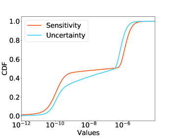
Figure 2: The cumulative distribution function (CDF) of $\overline{I}^{(t)}_{j}$ and $\overline{U}^{(t)}_{j}$ over $j$ at $t=500$ when pruning BERT-base on RTE.

We remark (9) shares the same spirit with UCB methods for bandit problems (Lai et al., 1985; Zhang et al., 2021). Each parameter is considered as an arm, $\overline{I}^{(t)}_{j}$ is regarded as estimated rewards and $\overline{U}^{(t)}_{j}$ controls the level of uncertainty. Since $\overline{I}^{(t)}_{j}$ and $\overline{U}^{(t)}_{j}$ are highly skewed to zero as shown by Figure 2, (9) applies a logarithmic transformation to make them distribute more evenly:

$$S^{(t)}_{j}=\exp\Big{(}\log(\overline{I}^{(t)}_{j})+c\log(\overline{U}^{(t)}_{j})\Big{)},$$

where we let $c=1$. The above equation aligns to the policy of UCB. The upper confidence bound $\overline{U}^{(t)}_{j}$ quantifies the uncertainty of importance estimation and promotes the exploration.

With our defined importance score, our algorithm prunes the model weights after each gradient decent step, i.e.,

$$\bm{\theta}^{(t+1)}=\mathcal{T}(\bm{\theta}^{(t)}-\alpha\nabla\mathcal{L}(\bm{\theta}^{(t)}),S^{(t)}),$$ (10)

where $\mathcal{T}$ is defined in (5). We summarize our proposed algorithm PLATON in Algorithm 1.

4 Experiments

We implement PLATON for pruning pre-trained BERT-base Devlin et al. (2019), DeBERTaV3-base He et al. (2021b) and ViT-B16 Dosovitskiy et al. (2020) during fine-tuning. We evaluate effectiveness of the proposed algorithm on natural language understanding (GLUE, Wang et al. 2019), question answer (SQuAD v1.1, Rajpurkar et al. 2016b) and image classification (CIFAR100, Krizhevsky et al. 2009; ImageNet, Deng et al. 2009) tasks. All the gains have passed significance tests with $p<0.05$.

Implementation details. We use PyTorch (Paszke et al., 2019) to implement all the algorithms. Our implementation is based on the publicly available MT-DNN (Liu et al., 2019a, 2020) and Huggingface Transformers (Wolf et al., 2019) code-base. All the experiments are conducted on NVIDIA V100 GPUs.

In Algorithm 1, a weight may be zeroed-out (pruned) and reactivated in later iterations. In this case, we let the weight starts from zero instead of from the value before zeroing-out. This is because a pruned weight is still included in the training dynamics as a zero value, such that its is natural to restart it from zero.

We use a cubic schedule Zhu and Gupta (2018); Sanh et al. (2020); Zafrir et al. (2021) to gradually increase the sparsity level during pruning. Please refer to Appendix A for details.

Baselines. We compare PLATON with the following methods:

$\bullet$ $\ell_{0}$ regularization (Louizos et al., 2018) is an effective modeling pruning method. The method adds a penalty to the proportion of remaining weights.

$\bullet$ Magnitude pruning (Zhu and Gupta, 2018) propose an automated gradual pruning method, which is a magnitude-based pruning method. The method enables masked weights to be updated, and has achieved state-of-the-art results among magnitude-based approaches.

$\bullet$ Movement pruning (Sanh et al., 2020) is a state-of-the-art method for model pruning. The method applies an iterative pruning strategy, where sensitivity is used as the importance metric. The approach considers the changes in weights during training, and has achieved superior performance.

$\bullet$ Soft movement pruning (Sanh et al., 2020) is a soft version of movement pruning based on the binary mask function in Mallya and Lazebnik (2018).

We use publicly available implementation to run all the baselines. Please refer to Sanh et al. (2020) and references therein for more details.

Table 1: Results with BERT-base on GLUE development set. Here Ratio is the proportion of remaining weights. Results with N.A. indicate the model does not converge. The best results on each dataset are shown in bold. We report mean of $5$ runs using different random seeds.

Ratio	Method	MNLI	RTE	QNLI	MRPC	QQP	SST-2	CoLA	STS-B
		m / mm	Acc	Acc	Acc / F1	Acc / F1	Acc	Mcc	P/S Corr
100%	$\text{BERT}_{\text{base}}$	84.6 / 83.4	69.3	91.3	86.4 / 90.3	91.5 / 88.5	92.7	58.3	90.2 / 89.7
20%	$\ell_{0}$ Regularization	80.5 / 81.1	63.2	85.0	75.7 / 80.2	88.5 / 83.3	85.0	N.A.	82.8 / 84.7
	Magnitude	81.5 / 82.9	65.7	89.2	79.9 / 86.2	86.0 / 83.8	84.3	42.5	86.8 / 86.6
	Movement	80.6 / 80.8	N.A.	81.7	68.4 / 81.1	89.2 / 85.7	82.3	N.A.	N.A.
	Soft-Movement	81.6 / 82.1	62.8	88.3	80.9 / 86.7	90.6 / 87.5	89.0	48.5	87.8 / 87.5
	PLATON	83.1 / 83.4	68.6	90.1	85.5 / 89.8	90.7 / 87.5	91.3	54.5	89.0 / 88.5
15%	$\ell_{0}$ Regularization	79.1 / 79.8	62.5	84.0	74.8 / 79.8	87.9 / 82.3	82.8	N.A.	81.8 / 84.2
	Magnitude	80.1 / 80.7	64.6	88.0	69.6 / 79.4	83.6 / 79.2	82.8	N.A.	85.4 / 85.0
	Movement	80.1 / 80.3	N.A.	81.2	68.4 / 81.0	89.6 / 86.1	81.8	N.A.	N.A.
	Soft-Movement	81.2 / 81.7	60.2	87.2	81.1 / 87.0	90.4 / 87.1	88.4	40.8	86.9 / 86.6
	PLATON	82.7 / 83.0	65.7	89.9	85.3 / 89.5	90.5 / 87.3	91.1	52.5	88.4 / 87.9
10%	$\ell_{0}$ Regularization	78.0 / 78.7	59.9	82.8	73.8 / 79.5	87.6 / 82.0	82.5	N.A.	82.7 / 83.9
	Magnitude	78.8 / 79.0	57.4	86.6	70.3 / 80.3	78.8 / 77.0	80.7	N.A.	83.4 / 83.3
	Movement	79.3 / 79.5	N.A.	79.2	68.4 / 81.2	89.1 / 85.4	80.2	N.A.	N.A.
	Soft-Movement	80.7 / 81.1	58.8	86.6	79.7 / 85.9	90.2 / 86.7	87.4	N.A.	86.5 / 86.3
	PLATON	82.0 / 82.2	65.3	88.9	84.3 / 88.8	90.2 / 86.8	90.5	44.3	87.4 / 87.1

4.1 Natural Language Understanding

Models and Datasets. We evaluate the pruning performance of BERT-base (Devlin et al., 2019) and DeBERTaV3-base (He et al., 2021b) using the proposed algorithm. We conduct experiments on the General Language Understanding Evaluation (GLUE, Wang et al. 2019) benchmark. The benchmark includes two single-sentence classification tasks: SST-2 (Socher et al., 2013) and CoLA (Warstadt et al., 2019). GLUE also contains three similarity and paraphrase tasks: MRPC (Dolan and Brockett, 2005), STS-B (Cer et al., 2017) and QQP. There are also four natural language inference tasks in GLUE: MNLI (Williams et al., 2018); QNLI (Rajpurkar et al., 2016a); RTE (Dagan et al., 2006; Bar-Haim et al., 2006; Giampiccolo et al., 2007; Bentivogli et al., 2009); and WNLI (Levesque et al., 2012). Following previous works, we exclude WNLI in the experiments. Dataset details are summarized in Appendix B.

Implementation Details. We select the exponential moving average parameters $\beta_{1}$ from $\{0.75,0.80,\\ 0.85,0.90\}$ and $\beta_{2}$ from $\{0.850,0.900,0.950,0.975\}$. We select the learning rate from $\{3\times 10^{-5},5\times 10^{-5},8\times 10^{-5},1\times 10^{-4}\}$ and the batch size from $\{8,16,32\}$. More details are presented in Appendix C.

Main results. We compare PLATON with the baseline methods under different sparsity levels: $90\%$, $85\%$ and $80\%$. Table 1 shows experimental results on the GLUE development set. We see that PLATON achieves better or on par performance compared with existing approaches on all the datasets under all the sparsity levels. For example, when the sparsity level is $80\%$, PLATON achieves a $83.1\%$ accuracy on the MNLI-m dataset, which is $1.5\%$ higher than the best-performing baseline (soft movement pruning). The performance gain of our method is even more significant on small datasets. For example, PLATON outperforms existing approaches by more than $5\%$ on RTE when the sparsity level is $80\%$. We remark that while movement pruning and its soft version perform well on large datasets (e.g., MNLI and QQP), it behaves poorly or even cannot converge on small datasets (e.g., RTE, CoLA and STS-B). We provide plausible explanations in Section 6.

Table 2 summarizes experimental results on MNLI and SST-2 for pruning DeBERTaV3-base. Similar to Table 1, PLATON significantly outperforms the baseline method on all the datasets under all the sparsity levels. From the results, we see that for the DeBERTa model, our method obtains more performance gain when the sparsity level is high. For example, in the $70\%$ sparse case, PLATON outperforms the baseline by $1.9\%$ ($94.6$ v.s. $92.7$) on the SST-2 dataset; while in the $90\%$ sparse case, our method achieves a $6.6\%$ improvement ($90.0$ v.s. $83.4$).

Table 2: Results with DeBERTaV3-base on SQuAD v1.1, MNLI and SST-2. Here Ratio is the proportion of remaining weights. The best results on each dataset are shown in bold.

Ratio	Method	MNLI	SST-2	SQuAD
		m / mm	Acc	EM / F1
100%	$\text{BERT}_{\text{base}}$	89.9 / 90.1	95.6	84.6 / 92.0
30%	Magnitude	87.6 / 87.3	92.7	82.2 / 89.9
	PLATON	88.9 / 88.8	94.6	83.1 / 90.9
20%	Magnitude	82.3 / 83.8	90.8	78.8 / 86.7
	PLATON	87.2 / 87.0	93.1	81.9 / 89.8
15%	Magnitude	80.7 / 81.0	88.5	75.8 / 84.6
	PLATON	85.8 / 85.9	92.3	81.2 / 89.0
10%	Magnitude	77.1 / 78.0	83.4	70.5 / 80.5
	PLATON	83.4 / 83.5	90.0	79.0 / 87.1

4.2 Question Answering

Models and Datasets. We evaluate performance of the proposed algorithm on a question answering dataset (SQuAD v1.1, Rajpurkar et al. 2016a), where we use PLATON to prune BERT-base and DeBERTaV3-base. Question answering is treated as a sequence labeling problem, where we predict the probability of each token being the start and end of the answer span. The dataset contains $88k$ training and $10k$ validation samples.

Implementation Details. We set the batch size as $16$, and the number of epochs for fine-tuning as $10$. We use AdamW (Loshchilov and Hutter, 2019) as the optimizer and we set the learning rate as $3\times 10^{-5}$. Please refer to Appendix D for more details.

Main Results. Table 3 summarizes experimental results, where we prune a pre-trained BERT-base model under $6$ different sparsity settings. From the results, we see that PLATON consistently outperforms existing approaches under all sparsity levels in terms of the two evaluation metrics: exact match (EM) and F1. Notice that movement pruning and soft movement pruning are more efficient in the high-sparsity regime (e.g., $90\%$ sparse); while in the low-sparsity regime (e.g., $50\%$ sparse), these methods behave on par or worse than magnitude pruning and $\ell_{0}$ regularization. Our method, on the other hand, is effective under all sparsity levels. Also note that PLATON is more effective in the high-sparsity regime. For example, in the $50\%$ sparse case, our method outperforms the best-performing baseline (magnitude pruning) by $0.2\%$ in terms of F1; while in the $85\%$ sparse case, PLATON achieves a $2.5\%$ gain.

Table 2 summarizes results of pruning DeBERTaV3-base on the SQuAD v1.1 dataset. Similar to the findings in Table 3, PLATON significantly outperforms the baseline method. Additionally, our method is also more effective in the high-sparsity regime when pruning DeBERTa models.

Table 3: Results with $\text{BERT}_{\text{base}}$ on SQuAD v1.1. We report EM/F1. Here Ratio is the proportion of remaining weights. The best results in each setting are shown in bold.

Ratio	10%	15%	20%	30%	40%	50%
$\text{BERT}_{\text{base}}$	80.4 / 88.1
$\ell_{0}$ Regularization	68.9 / 80.0	70.7 / 80.9	72.0 / 81.9	73.1 / 82.8	74.3 / 83.9	75.1 / 84.6
Magnitude	67.7 / 78.2	73.4 / 82.9	75.9 / 84.8	77.4 / 86.5	77.9 / 86.7	78.5 / 87.0
Movement	71.9 / 81.9	72.1 / 81.8	72.3 / 82.0	71.6 / 81.9	72.7 / 82.8	73.4 / 83.0
Soft-Movement	71.0 / 81.0	72.2 / 82.2	–	75.3 / 84.6	–	77.0 / 85.8
PLATON	74.2 / 83.8	75.9 / 85.4	76.8 / 86.1	77.5 / 86.7	78.0 / 86.9	78.5 / 87.2

4.3 Image Classification

Models and Datasets. We apply PLATON to prune a ViT-B16 model (Dosovitskiy et al., 2020), and we evaluate model performance on two image classification datasets: CIFAR100 Krizhevsky et al. (2009) and ImageNet Deng et al. (2009).

Implementation Details. We implement ViT using the following codebase. We use SGD with momentum Qian (1999) as the optimizer. For CIFAR100, we set the batch size as $512$ and the learning rate as $0.03$. For ImageNet, we set the batch size as $150$ and the learning rate as $0.03$. Detailed settings are deferred to Appendix E.

Main Results. Experimental results are summarized in Table 4. We see that our method significantly outperforms existing methods on both the datasets (CIFAR100 and ImageNet) under all the sparsity levels. For example, the accuracy of PLATON is $76.3\%$ on ImageNet when the sparsity level is $80\%$, whereas the accuracy of magnitude pruning and movement pruning is only $66.5\%$ and $66.6\%$, respectively. Note that performance gain of our method is more significant in the high sparsity regime.

Table 4: Results with ViT-B16 on CIFAR100 and ImageNet. Here Ratio is the proportion of remaining weights. The best results on each dataset are shown in bold.

	Ratio	Magnitude	Movement	PLATON	ViT-B16
CIFAR100	30%	88.9	78.5	90.1	92.3
	20%	84.6	78.6	87.3
	10%	64.3	77.5	81.2
ImageNet	40%	81.5	69.3	82.6	83.5
	30%	78.9	68.6	80.5
	20%	66.5	66.6	76.3

4.4 Analysis

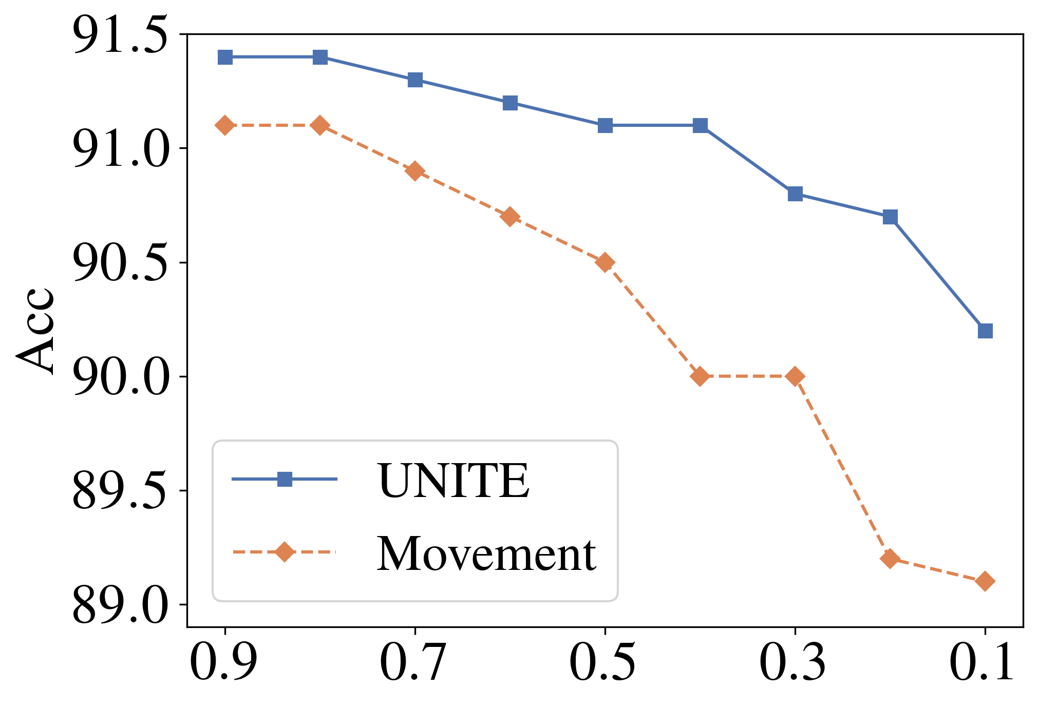
(a) QQP

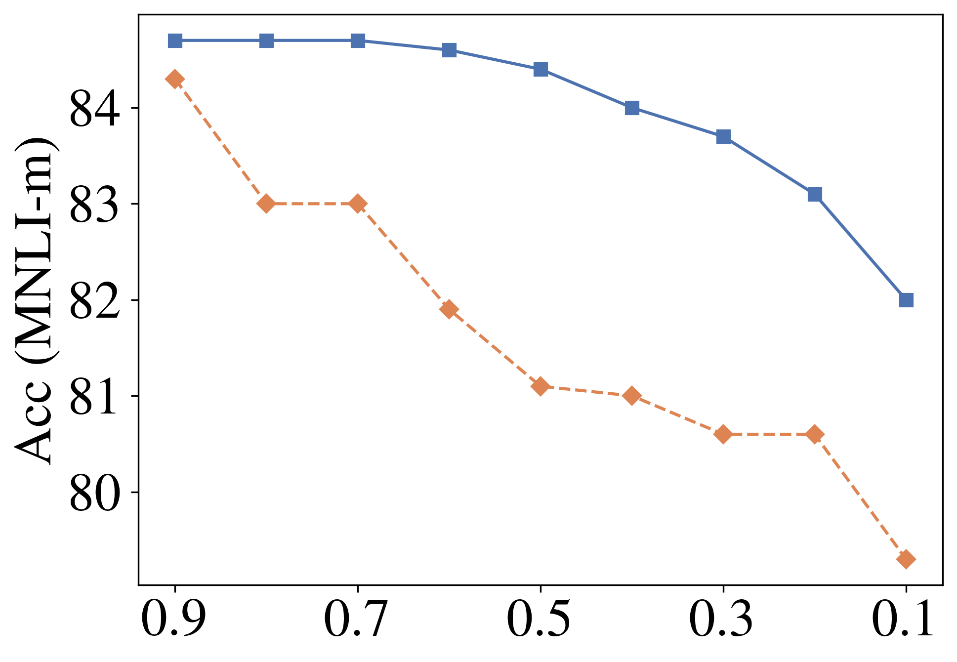
(b) MNLI-m

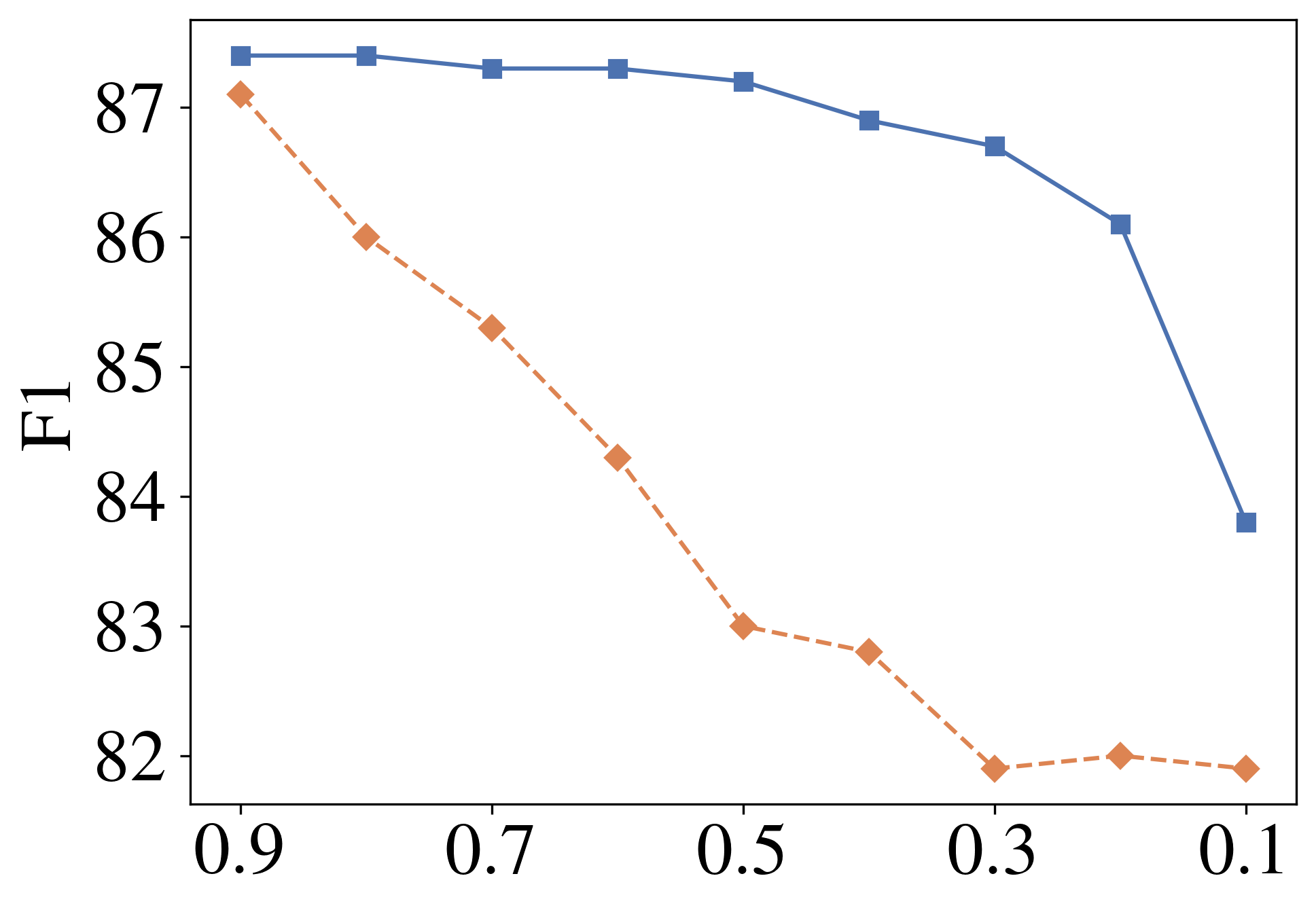
(c) SQuAD v1.1

Figure 3: Model performance under different pruning ratio. We prune a BERT-base model during fine-tuning. Here the $x$-axis is the proportion of remaining weights.

Different levels of pruning ratio. Figure 3 illustrates experimental results of pruning a BERT-base model during fine-tuning under different sparsity levels. We see that on all the three datasets (QQP, MNLI-m and SQuAD v1.1), PLATON achieves consistent performance improvement under all the sparsity levels compared with the baseline. Note that the performance gain is more significant when the sparsity level is high ($>50\%$). For example, PLATON outperforms the baseline by $0.4\%$ on MNLI-m when the sparsity level is $10\%$; while our method achieves a more than $3.0\%$ gain in accuracy when the sparsity level is $70\%$.

Variants of the importance score. Recall that in PLATON, the importance score is the product of sensitivity and uncertainty ($S=\overline{I}\odot\overline{U}$). In Table 5, we examine variants of the importance score. From the results, we see that using only the sensitivity ($S=\overline{I}$) or the uncertainty ($S=\overline{U}$) deteriorates model performance by over $1.0\%$ on all the three datasets. We also examine the case where $S=\overline{I}/\overline{U}$, i.e., we prune the weights with large uncertainty. In this case, the model fails to converge on CoLA, and the model performance drastically drops on the other datasets (i.e., $8.6\%$ on RTE and $9.6\%$ on SST-2). This indicates that weights with high uncertainty should be retained and further explored.

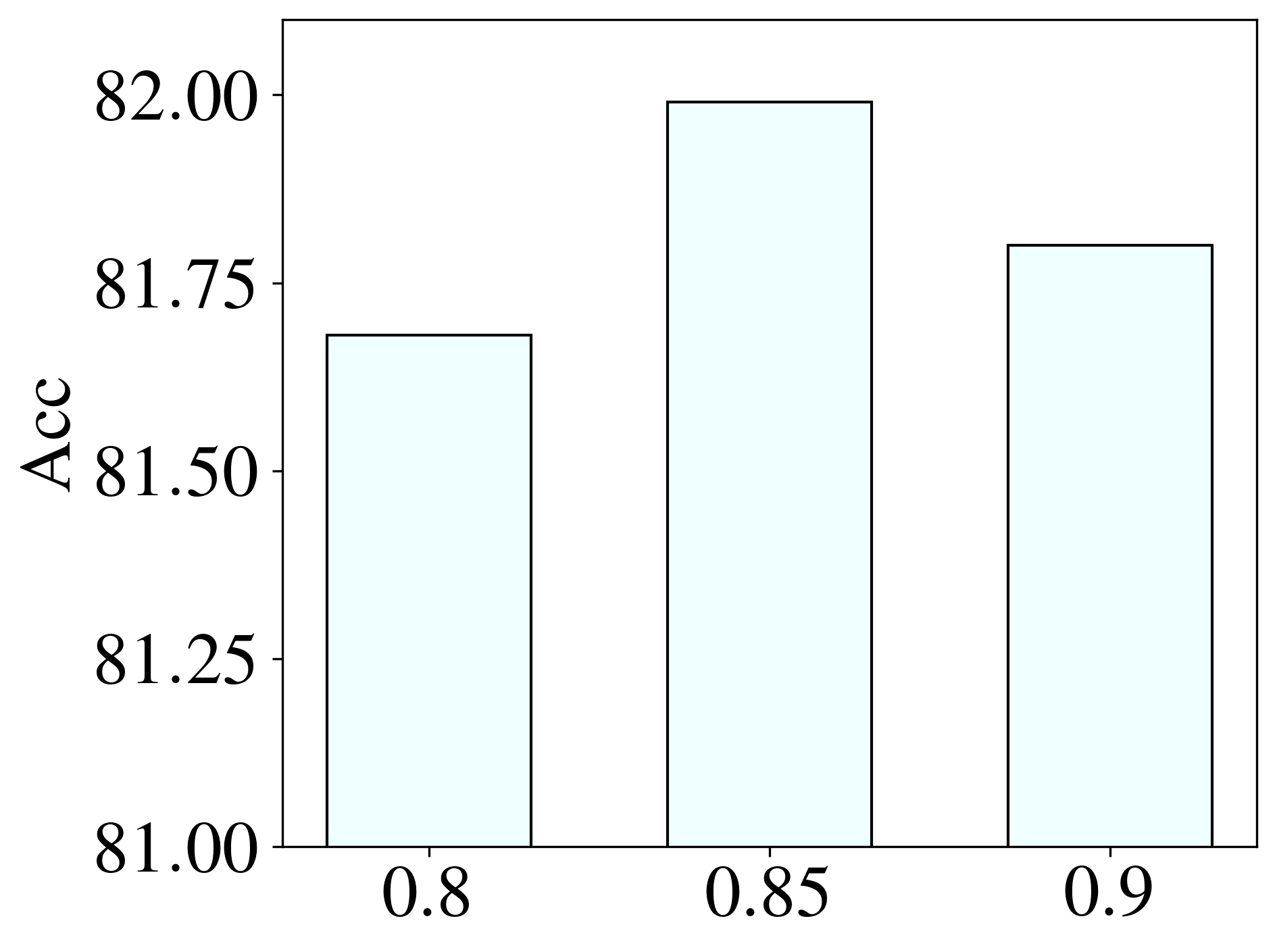
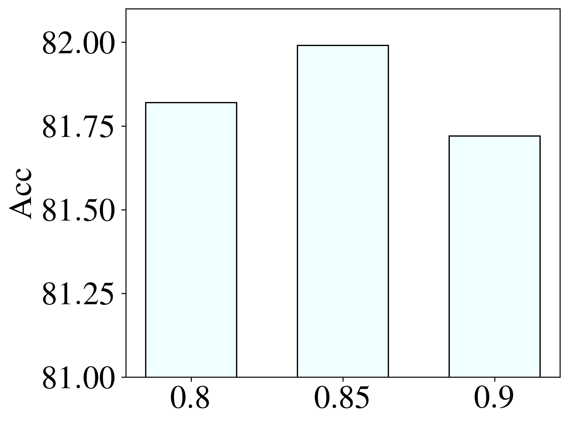
Figure 4: Results on MNLI-m under different exponential moving average parameters. Left: $\beta_{1}$; Right: $\beta_{2}$. By default, we set $\beta_{1}=0.85$ and $\beta_{2}=0.85$.

Table 5: Variants of the importance score. We prune a BERT-base model.

	SST-2	RTE	CoLA
PLATON	90.5	65.3	44.3
$S=\overline{I}$	89.4	63.6	42.8
$S=\overline{U}$	89.3	64.3	40.6
$S=\overline{I}/\overline{U}$	80.9	56.7	N.A.

Sensitivity to exponential moving average. Table 4 summarizes experimental results when we change the exponential moving average parameters $\beta_{1}$ and $\beta_{2}$. In these experiments, we prune a pre-trained BERT-base model on the MNLI-m dataset. From the results, we see that our method is robust to these two hyper-parameters. In practice we fix $\beta_{1}=\beta_{2}=0.85$. Even when these selected hyper-parameters are not optimal, performance of PLATON is still better than the baseline methods.

5 Extension to Structured Pruning

Algorithm 1 targets on unstructured pruning (LeCun et al., 1990; Han et al., 2015b; Frankle and Carbin, 2019; Sanh et al., 2020), which prunes model weights entry-wise. However, it is notoriously difficult to speedup inference of the pruned model, which requires low-level implementation that is not supported by existing deep learning libraries such as PyTorch (Paszke et al., 2019) and Tensorflow (Abadi et al., 2016). In contrast, structured pruning (McCarley et al., 2019; Fan et al., 2020; Sajjad et al., 2020; Lagunas et al., 2021) methods remove columns or blocks of the weights, such that the pruned model can be easily compressed. As such, inference speedup via structured pruning is more implementation-friendly.

5.1 Uncertainty Adjusted Structured Pruning

Our method can be extended to structured pruning. In this case, the proposed importance score is computed group-wise instead of entry-wise (c.f. (9)). Specifically, we divided the parameter $\bm{\theta}$ into $p$ disjoint groups denoted by

$$\bm{\theta}=\{\bm{\theta}_{\mathcal{G}_{1}},\bm{\theta}_{\mathcal{G}_{2}},\dots,\bm{\theta}_{\mathcal{G}_{p}}\}.$$

For example, for a weight matrix, $\mathcal{G}_{j}$ can denote its $j$-th column. Then the sensitivity of $\bm{\theta}_{\mathcal{G}_{j}}$ is defined as

$$I_{\mathcal{G}_{j}}=\left|\bm{\theta}_{\mathcal{G}_{j}}^{\top}\nabla_{\mathcal{G}_{j}}\mathcal{L}(\bm{\theta})\right|.$$ (11)

We apply exponential moving average to smooth the sensitivity of each group:

$$\overline{I}^{(t+1)}_{\mathcal{G}_{j}}=\beta_{1}\overline{I}^{(t)}_{\mathcal{G}_{j}}+(1-\beta_{1})I^{(t)}_{\mathcal{G}_{j}}.$$

Similar to (7) and (8), we quantify the uncertainty of sensitivity of each group and then apply exponential moving average as the following:

$$U^{(t)}_{\mathcal{G}_{j}}=\left|I^{(t)}_{\mathcal{G}_{j}}-\overline{I}^{(t)}_{\mathcal{G}_{j}}\right|,\quad\overline{U}^{(t+1)}_{\mathcal{G}_{j}}=\beta_{2}\overline{U}^{(t)}_{\mathcal{G}_{j}}+(1-\beta_{2})U^{(t)}_{\mathcal{G}_{j}}.$$

The importance score is defined as (c.f. (9))

$$S^{(t)}_{\mathcal{G}_{j}}=\overline{I}^{(t)}_{\mathcal{G}_{j}}\cdot\overline{U}^{(t)}_{\mathcal{G}_{j}}.$$

We prune the model using (5) in a group fashion, i.e., we zero-out the entire group $\bm{\theta}_{\mathcal{G}_{j}}$ if $S^{(t)}_{\mathcal{G}_{j}}$ is not in top-$r$%.

Table 6: Results with $\text{BERT}_{\text{base}}$ on SQuAD v1.1. We report EM/F1. Here Ratio is the proportion of remaining weights.

Ratio	PLATON	PLATONstructure
40%	78.0 / 86.9	75.6 / 84.9
50%	78.5 / 87.2	77.0 / 85.9

5.2 Experimental Results

We evaluate performance of the proposed structured pruning method by pruning BERT-base on SQuAD v1.1. Table 6 summarizes experimental results. It is expected that performance of structured pruning is lower than the unstructured alternative, because we have less control over individual weights. For example, important weights and unimportant ones may locate in the same column and are pruned together. From the results, we see that performance of PLATON_structure drops by about $1.5$ and $2.0$ when the sparsity levels are $50\%$ and $60\%$, respectively.

6 Discussion

Movement pruning (Sanh et al., 2020) is one of the most popular model pruning methods. However, empirically we observe that it suffers from training instability and even divergence. This might be due to the following reasons:

First, as mentioned earlier, the importance scores (sensitivity) estimated on mini-batches have high variability in movement pruning. This causes training instability as a weight may frequently alternates between being retained and being pruned. By considering uncertainty of the importance estimation, variability of importance scores in PLATON is drastically smaller (Figure 1, bottom), yielding a more stable training process and better model performance.

Second, a weight is masked instead of zeroed-out when it is deemed unimportant in movement pruning. Subsequently, if the rank of the weight’s importance score raises in later iterations, it is unmasked and its value is restored. However, the may be a number of iterations between a weight being masked and being reactivated, such that the weight’s value becomes stale. In this case, such a stale weight can have a huge influence to the model, rendering training unstable. In contrast, in PLATON, we let a weight starts from zero when reactivated. This is natural because a pruned weight is still included in the training dynamics as a zero value.

7 Conclusion

We propose PLATON, which is a model pruning algorithm that considers both sensitivity of model weights and uncertainty of importance estimation. In PLATON, we use exponential moving average to smooth the sensitivity computed on mini-batches. Moreover, we quantify uncertainty of the importance estimation via the local temporal variation. These approaches effectively reduce variability of the importance score (smoothed sensitivity times uncertainty) and stabilize training. We conduct extensive experiments on natural language understanding, question answering and image classification. Results show that PLATON significantly outperforms existing approaches. Our approach is particularly effective in the high sparsity regime. For example, when pruning DeBERTaV3-base on the SQuAD v1.1 dataset, our method achieves a more than $5.0\%$ improvement when $90\%$ of the weights are pruned. Moreover, training of PLATON is more stable and less sensitive to the hyper-parameters.

Appendix A Sparsity Ratio Schedule

The cubic schedule of sparsity ratio is widely applied by many existing methods (Zhu and Gupta, 2018; Sanh et al., 2020; Zafrir et al., 2021), which includes initial and final warmups:

$$r^{(t)}=\begin{cases}r^{(0)}&0\leq t<t_{i}\\ r^{(T)}+\left(r^{(0)}-r^{(T)}\right)\left(1-\frac{t-t_{i}-t_{f}}{T-t_{i}-t_{f}}\right)^{3}&t_{i}\leq t<T-t_{f}\\ r^{(T)}&\text{ o.w. }\end{cases}$$ (12)

Same as Sanh et al. (2020), we applies this cubic schedule to all baseline methods and our algorithm.

Appendix B GLUE Dataset Statistics

We present the dataset statistics of GLUE (Wang et al., 2019) in the following table.

Corpus	Task	#Train	#Dev	#Test	#Label	Metrics
Single-Sentence Classification (GLUE)
CoLA	Acceptability	8.5k	1k	1k	2	Matthews corr
SST	Sentiment	67k	872	1.8k	2	Accuracy
Pairwise Text Classification (GLUE)
MNLI	NLI	393k	20k	20k	3	Accuracy
RTE	NLI	2.5k	276	3k	2	Accuracy
QQP	Paraphrase	364k	40k	391k	2	Accuracy/F1
MRPC	Paraphrase	3.7k	408	1.7k	2	Accuracy/F1
QNLI	QA/NLI	108k	5.7k	5.7k	2	Accuracy
Text Similarity (GLUE)
STS-B	Similarity	7k	1.5k	1.4k	1	Pearson/Spearman corr

Table 7: Summary of the GLUE benchmark.

Appendix C Natural Language Understanding

C.1 Training Details

Implementation Details. The implementation of PLATON on BERT-base is based on publicly available MT-DNN (Liu et al., 2019a, 2020) code-base. The implementation of DeBertaV3-base (He et al., 2021a) on GLUE is based on Huggingface Transformers (Wolf et al., 2019) code-base.

Hyper-parameter Details. We select $\beta_{1}$ in range of $\{0.75,0.80,0.85,0.90\}$, find $0.85$ generally perform best and fix it as $0.85$ for all experiments. We select $\beta_{2}$ from $\{0.850,0.900,0.950,0.975\}$. We choose AdamW as optimizer and select learning rate from $\{3\times 10^{-5},5\times 10^{-5},8\times 10^{-5},1\times 10^{-4}\}$ and batch size from $\{8,16,32\}$ and fix them for each dataset. Table 8 lists the detailed setup of each dataset. For baseline methods, we set the hyper-parameters all as reported by (Sanh et al., 2020).

We found that PLATON is not sensitive to its hyper-parameters $\beta_{1}$ and $\beta_{2}$. The performance of PLATON does not alter dramatically among different hyper-parameter setup.

Table 8: Hyper-parameter setup of PLATON for GLUE benchmark.

Ratio	Hyper-parameter	MNLI	RTE	QNLI	MRPC	QQP	SST-2	CoLA	STS-B
	# epochs	8	20	10	10	10	6	15	15
	Batch size	32	16	32	8	32	32	32	16
	Learning rate	$8\times 10^{-5}$	$1\times 10^{-4}$	$1\times 10^{-4}$	$1\times 10^{-4}$	$1\times 10^{-4}$	$8\times 10^{-5}$	$1\times 10^{-4}$	$1\times 10^{-4}$
20%	$t_{i}$	5400	200	2000	300	5400	1000	500	500
	$t_{f}$	22000	1200	12000	900	22000	5000	1500	2500
	$\beta_{1}$	0.85	0.85	0.85	0.85	0.85	0.85	0.85	0.85
	$\beta_{2}$	0.85	0.99	0.95	0.95	0.85	0.85	0.95	0.85
15%	$t_{i}$	5400	200	2000	300	5400	1000	500	500
	$t_{f}$	22000	1200	12000	900	22000	5000	1500	2500
	$\beta_{1}$	0.85	0.85	0.85	0.85	0.85	0.85	0.85	0.85
	$\beta_{2}$	0.90	0.50	0.90	0.95	0.90	0.90	0.975	0.90
10%	$t_{i}$	5400	200	2000	300	5400	1000	500	500
	$t_{f}$	22000	1200	12000	900	22000	5000	1500	2500
	$\beta_{1}$	0.85	0.85	0.85	0.85	0.85	0.85	0.85	0.85
	$\beta_{2}$	0.85	0.95	0.95	0.95	0.90	0.85	0.95	0.95

Appendix D Question Answering

D.1 Dataset

Following Sanh et al. (2020), we also choose SQuAD v1.1 (Rajpurkar et al., 2016b) to evaluate the performance of PLATON on question answering task.

D.2 Training Details

We set the batch size as 16, the number of epochs for fine-tuning as 10, the optimizer as AdamW and the learning rate as $3\times 10^{-5}$ for all algorithms. We select the number of epochs as 10. For PLATON, we set its cubic sparsity schedule as $t_{i}=5400$ and $t_{f}=22000$. The baselines are all configured as reported by Sanh et al. (2020). The other hyper-parameters are reported in Table 9.

Table 9: Hyper-parameter setup of PLATON on question answering tasks (SQuAD v1.1, Rajpurkar et al. (2016b)).

Ratio	10%	15%	20%	30%	40%	50%
$\beta_{1}$	0.85	0.85	0.85	0.85	0.85	0.85
$\beta_{2}$	0.975	0.975	0.975	0.975	0.900	0.975

Appendix E Image Classification

For all image classification tasks we use the Vision Transformer model (ViT) (Dosovitskiy et al., 2020). We use the base model with an input patch size of $16\times 16$. The ViT model is pre-trained on the Imagenet-21K dataset.

E.1 Datasets

We evaluate the PLATON method on two datasets, CIFAR-100 and the ILSVRC-2012 ImageNet dataset. The CIFAR-100 has 100 classes containing 600 images each. We use a image resolution of $224$ for CIFAR-100. There are 500 training images and 100 testing images per class. The ILSVRC-2012 ImageNet dataset contains 1.2 million images spanning 1000 categories. We use a image resolution of $384\times 384$ for ImageNet.

E.2 Training Details

Implementation Details. The implementation of ViT follows the codebase of its pytorch version. We use SGD with momentum (Qian, 1999) as optimizer. For CIFAR100, we set batch size as 512 and learning rate as $0.03$. For ImageNet, we set batch size as 150 and learning rate as 0.03.

Finetuning Details. We fine-tune the ViT model with a learning rate 0f 0.03. We use a batch size of 512 for CIFAR-100 and 150 for ImageNet due to memory constraints. In addition, we use gradient clipping at norm 1. We also use a cosine decay for the learning rate with a warmup of 1000 steps.

PLATON Details. We use the following hyperparameters for the PLATON algorithm. For the ImageNet dataset we use a $t_{i}=7000$ step warmup period, a $t_{f}=10000$ step final warmup period, and finetune for 60000 steps total. We set the exponential moving average parameter to 0.85.

For the CIFAR-100 dataset we use a 2000 step warmup period, a 8000 step final warmup period, and finetune for 20000 steps total. We set the exponential moving average parameter to 0.85.

References

- Abadi et al. (2016) Abadi, M., Barham, P., Chen, J., Chen, Z., Davis, A., Dean, J., Devin, M., Ghemawat, S., Irving, G., Isard, M. et al. (2016). Tensorflow: A system for large-scale machine learning. In 12th USENIX symposium on operating systems design and implementation (OSDI 16).
- Bar-Haim et al. (2006) Bar-Haim, R., Dagan, I., Dolan, B., Ferro, L. and Giampiccolo, D. (2006). The second PASCAL recognising textual entailment challenge. In Proceedings of the Second PASCAL Challenges Workshop on Recognising Textual Entailment.
- Behnke and Heafield (2021) Behnke, M. and Heafield, K. (2021). Pruning neural machine translation for speed using group lasso. In Proceedings of the Sixth Conference on Machine Translation.
- Bentivogli et al. (2009) Bentivogli, L., Dagan, I., Dang, H. T., Giampiccolo, D. and Magnini, B. (2009). The fifth pascal recognizing textual entailment challenge. In In Proc Text Analysis Conference (TAC’09.
- Brown et al. (2020) Brown, T. B., Mann, B., Ryder, N., Subbiah, M., Kaplan, J., Dhariwal, P., Neelakantan, A., Shyam, P., Sastry, G., Askell, A., Agarwal, S., Herbert-Voss, A., Krueger, G., Henighan, T., Child, R., Ramesh, A., Ziegler, D. M., Wu, J., Winter, C., Hesse, C., Chen, M., Sigler, E., Litwin, M., Gray, S., Chess, B., Clark, J., Berner, C., McCandlish, S., Radford, A., Sutskever, I. and Amodei, D. (2020). Language models are few-shot learners. In Advances in Neural Information Processing Systems 33: Annual Conference on Neural Information Processing Systems 2020, NeurIPS 2020, December 6-12, 2020, virtual (H. Larochelle, M. Ranzato, R. Hadsell, M. Balcan and H. Lin, eds.).
- Cer et al. (2017) Cer, D., Diab, M., Agirre, E., Lopez-Gazpio, I. and Specia, L. (2017). SemEval-2017 task 1: Semantic textual similarity multilingual and crosslingual focused evaluation. In Proceedings of the 11th International Workshop on Semantic Evaluation (SemEval-2017). Association for Computational Linguistics, Vancouver, Canada.
- Chen et al. (2020) Chen, T., Frankle, J., Chang, S., Liu, S., Zhang, Y., Wang, Z. and Carbin, M. (2020). The lottery ticket hypothesis for pre-trained BERT networks. In Advances in Neural Information Processing Systems 33: Annual Conference on Neural Information Processing Systems 2020, NeurIPS 2020, December 6-12, 2020, virtual (H. Larochelle, M. Ranzato, R. Hadsell, M. Balcan and H. Lin, eds.).
- Dagan et al. (2006) Dagan, I., Glickman, O. and Magnini, B. (2006). The pascal recognising textual entailment challenge. In Proceedings of the First International Conference on Machine Learning Challenges: Evaluating Predictive Uncertainty Visual Object Classification, and Recognizing Textual Entailment. MLCW’05, Springer-Verlag, Berlin, Heidelberg.
- Deng et al. (2009) Deng, J., Dong, W., Socher, R., Li, L., Li, K. and Li, F. (2009). Imagenet: A large-scale hierarchical image database. In 2009 IEEE Computer Society Conference on Computer Vision and Pattern Recognition (CVPR 2009), 20-25 June 2009, Miami, Florida, USA. IEEE Computer Society.
- Devlin et al. (2019) Devlin, J., Chang, M.-W., Lee, K. and Toutanova, K. (2019). BERT: Pre-training of deep bidirectional transformers for language understanding. In Proceedings of the 2019 Conference of the North American Chapter of the Association for Computational Linguistics: Human Language Technologies, Volume 1 (Long and Short Papers). Association for Computational Linguistics, Minneapolis, Minnesota.
- Ding et al. (2019) Ding, X., Ding, G., Zhou, X., Guo, Y., Han, J. and Liu, J. (2019). Global sparse momentum SGD for pruning very deep neural networks. In Advances in Neural Information Processing Systems 32: Annual Conference on Neural Information Processing Systems 2019, NeurIPS 2019, December 8-14, 2019, Vancouver, BC, Canada (H. M. Wallach, H. Larochelle, A. Beygelzimer, F. d’Alché-Buc, E. B. Fox and R. Garnett, eds.).
- Dolan and Brockett (2005) Dolan, W. B. and Brockett, C. (2005). Automatically constructing a corpus of sentential paraphrases. In Proceedings of the Third International Workshop on Paraphrasing (IWP2005).
- Dosovitskiy et al. (2020) Dosovitskiy, A., Beyer, L., Kolesnikov, A., Weissenborn, D., Zhai, X., Unterthiner, T., Dehghani, M., Minderer, M., Heigold, G., Gelly, S. et al. (2020). An image is worth 16x16 words: Transformers for image recognition at scale. arXiv preprint arXiv:2010.11929.
- Fan et al. (2020) Fan, A., Grave, E. and Joulin, A. (2020). Reducing transformer depth on demand with structured dropout. In 8th International Conference on Learning Representations, ICLR 2020, Addis Ababa, Ethiopia, April 26-30, 2020. OpenReview.net.
- Frankle and Carbin (2019) Frankle, J. and Carbin, M. (2019). The lottery ticket hypothesis: Finding sparse, trainable neural networks. In 7th International Conference on Learning Representations, ICLR 2019, New Orleans, LA, USA, May 6-9, 2019. OpenReview.net.
- Giampiccolo et al. (2007) Giampiccolo, D., Magnini, B., Dagan, I. and Dolan, B. (2007). The third PASCAL recognizing textual entailment challenge. In Proceedings of the ACL-PASCAL Workshop on Textual Entailment and Paraphrasing. Association for Computational Linguistics, Prague.
- Han et al. (2016) Han, S., Liu, X., Mao, H., Pu, J., Pedram, A., Horowitz, M. A. and Dally, W. J. (2016). Eie: Efficient inference engine on compressed deep neural network. ACM SIGARCH Computer Architecture News, 44 243–254.
- Han et al. (2015a) Han, S., Mao, H. and Dally, W. J. (2015a). Deep compression: Compressing deep neural networks with pruning, trained quantization and huffman coding. arXiv preprint arXiv:1510.00149.
- Han et al. (2015b) Han, S., Pool, J., Tran, J. and Dally, W. J. (2015b). Learning both weights and connections for efficient neural network. In Advances in Neural Information Processing Systems 28: Annual Conference on Neural Information Processing Systems 2015, December 7-12, 2015, Montreal, Quebec, Canada (C. Cortes, N. D. Lawrence, D. D. Lee, M. Sugiyama and R. Garnett, eds.).
- He et al. (2021a) He, P., Gao, J. and Chen, W. (2021a). Debertav3: Improving deberta using electra-style pre-training with gradient-disentangled embedding sharing. arXiv preprint arXiv:2111.09543.
- He et al. (2021b) He, P., Liu, X., Gao, J. and Chen, W. (2021b). Deberta: Decoding-enhanced bert with disentangled attention. In International Conference on Learning Representations.
- Krizhevsky (2009) Krizhevsky, A. (2009). Learning multiple layers of features from tiny images. Tech. rep.
- Krizhevsky et al. (2009) Krizhevsky, A., Hinton, G. et al. (2009). Learning multiple layers of features from tiny images.
- Lagunas et al. (2021) Lagunas, F., Charlaix, E., Sanh, V. and Rush, A. M. (2021). Block pruning for faster transformers. arXiv preprint arXiv:2109.04838.
- Lai et al. (1985) Lai, T. L., Robbins, H. et al. (1985). Asymptotically efficient adaptive allocation rules. Advances in applied mathematics, 6 4–22.
- LeCun et al. (1990) LeCun, Y., Denker, J. S. and Solla, S. A. (1990). Optimal brain damage. In Advances in neural information processing systems.
- Lee et al. (2019) Lee, N., Ajanthan, T. and Torr, P. H. S. (2019). Snip: single-shot network pruning based on connection sensitivity. In 7th International Conference on Learning Representations, ICLR 2019, New Orleans, LA, USA, May 6-9, 2019. OpenReview.net.
- Levesque et al. (2012) Levesque, H., Davis, E. and Morgenstern, L. (2012). The winograd schema challenge. In Thirteenth International Conference on the Principles of Knowledge Representation and Reasoning.
- Liang et al. (2021) Liang, C., Zuo, S., Chen, M., Jiang, H., Liu, X., He, P., Zhao, T. and Chen, W. (2021). Super tickets in pre-trained language models: From model compression to improving generalization. In Proceedings of the 59th Annual Meeting of the Association for Computational Linguistics and the 11th International Joint Conference on Natural Language Processing (Volume 1: Long Papers). Association for Computational Linguistics, Online.
- Liu et al. (2019a) Liu, X., He, P., Chen, W. and Gao, J. (2019a). Multi-task deep neural networks for natural language understanding. In Proceedings of the 57th Annual Meeting of the Association for Computational Linguistics. Association for Computational Linguistics, Florence, Italy.
- Liu et al. (2020) Liu, X., Wang, Y., Ji, J., Cheng, H., Zhu, X., Awa, E., He, P., Chen, W., Poon, H., Cao, G. and Gao, J. (2020). The Microsoft toolkit of multi-task deep neural networks for natural language understanding. In Proceedings of the 58th Annual Meeting of the Association for Computational Linguistics: System Demonstrations. Association for Computational Linguistics, Online.
- Liu et al. (2019b) Liu, Y., Ott, M., Goyal, N., Du, J., Joshi, M., Chen, D., Levy, O., Lewis, M., Zettlemoyer, L. and Stoyanov, V. (2019b). Roberta: A robustly optimized bert pretraining approach. arXiv preprint arXiv:1907.11692.
- Loshchilov and Hutter (2019) Loshchilov, I. and Hutter, F. (2019). Decoupled weight decay regularization. In 7th International Conference on Learning Representations, ICLR 2019, New Orleans, LA, USA, May 6-9, 2019. OpenReview.net.
- Louizos et al. (2018) Louizos, C., Welling, M. and Kingma, D. P. (2018). Learning sparse neural networks through l_0 regularization. In 6th International Conference on Learning Representations, ICLR 2018, Vancouver, BC, Canada, April 30 - May 3, 2018, Conference Track Proceedings. OpenReview.net.
- Mallya and Lazebnik (2018) Mallya, A. and Lazebnik, S. (2018). Piggyback: Adding multiple tasks to a single, fixed network by learning to mask. arXiv preprint arXiv:1801.06519, 6.
- McCarley et al. (2019) McCarley, J., Chakravarti, R. and Sil, A. (2019). Structured pruning of a bert-based question answering model. arXiv preprint arXiv:1910.06360.
- Molchanov et al. (2019) Molchanov, P., Mallya, A., Tyree, S., Frosio, I. and Kautz, J. (2019). Importance estimation for neural network pruning. In IEEE Conference on Computer Vision and Pattern Recognition, CVPR 2019, Long Beach, CA, USA, June 16-20, 2019. Computer Vision Foundation / IEEE.
- Molchanov et al. (2017) Molchanov, P., Tyree, S., Karras, T., Aila, T. and Kautz, J. (2017). Pruning convolutional neural networks for resource efficient inference. In 5th International Conference on Learning Representations, ICLR 2017, Toulon, France, April 24-26, 2017, Conference Track Proceedings. OpenReview.net.
- Paganini and Forde (2020) Paganini, M. and Forde, J. (2020). On iterative neural network pruning, reinitialization, and the similarity of masks. arXiv preprint arXiv:2001.05050.
- Paszke et al. (2019) Paszke, A., Gross, S., Massa, F., Lerer, A., Bradbury, J., Chanan, G., Killeen, T., Lin, Z., Gimelshein, N., Antiga, L., Desmaison, A., Köpf, A., Yang, E., DeVito, Z., Raison, M., Tejani, A., Chilamkurthy, S., Steiner, B., Fang, L., Bai, J. and Chintala, S. (2019). Pytorch: An imperative style, high-performance deep learning library. In Advances in Neural Information Processing Systems 32: Annual Conference on Neural Information Processing Systems 2019, NeurIPS 2019, December 8-14, 2019, Vancouver, BC, Canada (H. M. Wallach, H. Larochelle, A. Beygelzimer, F. d’Alché-Buc, E. B. Fox and R. Garnett, eds.).
- Qian (1999) Qian, N. (1999). On the momentum term in gradient descent learning algorithms. Neural networks, 12 145–151.
- Radford et al. (2019) Radford, A., Wu, J., Child, R., Luan, D., Amodei, D., Sutskever, I. et al. (2019). Language models are unsupervised multitask learners. OpenAI blog, 1 9.
- Rajpurkar et al. (2016a) Rajpurkar, P., Zhang, J., Lopyrev, K. and Liang, P. (2016a). SQuAD: 100,000+ questions for machine comprehension of text. In Proceedings of the 2016 Conference on Empirical Methods in Natural Language Processing. Association for Computational Linguistics, Austin, Texas.
- Rajpurkar et al. (2016b) Rajpurkar, P., Zhang, J., Lopyrev, K. and Liang, P. (2016b). SQuAD: 100,000+ questions for machine comprehension of text. In Proceedings of the 2016 Conference on Empirical Methods in Natural Language Processing. Association for Computational Linguistics, Austin, Texas.
- Renda et al. (2020) Renda, A., Frankle, J. and Carbin, M. (2020). Comparing rewinding and fine-tuning in neural network pruning. In 8th International Conference on Learning Representations, ICLR 2020, Addis Ababa, Ethiopia, April 26-30, 2020. OpenReview.net.
- Sajjad et al. (2020) Sajjad, H., Dalvi, F., Durrani, N. and Nakov, P. (2020). Poor man’s bert: Smaller and faster transformer models. arXiv e-prints arXiv–2004.
- Sanh et al. (2020) Sanh, V., Wolf, T. and Rush, A. M. (2020). Movement pruning: Adaptive sparsity by fine-tuning.
- Socher et al. (2013) Socher, R., Perelygin, A., Wu, J., Chuang, J., Manning, C. D., Ng, A. and Potts, C. (2013). Recursive deep models for semantic compositionality over a sentiment treebank. In Proceedings of the 2013 Conference on Empirical Methods in Natural Language Processing. Association for Computational Linguistics, Seattle, Washington, USA.
- Wang et al. (2019) Wang, A., Singh, A., Michael, J., Hill, F., Levy, O. and Bowman, S. R. (2019). GLUE: A multi-task benchmark and analysis platform for natural language understanding. In 7th International Conference on Learning Representations, ICLR 2019, New Orleans, LA, USA, May 6-9, 2019. OpenReview.net.
- Warstadt et al. (2019) Warstadt, A., Singh, A. and Bowman, S. R. (2019). Neural network acceptability judgments. Transactions of the Association for Computational Linguistics, 7 625–641.
- Williams et al. (2018) Williams, A., Nangia, N. and Bowman, S. (2018). A broad-coverage challenge corpus for sentence understanding through inference. In Proceedings of the 2018 Conference of the North American Chapter of the Association for Computational Linguistics: Human Language Technologies, Volume 1 (Long Papers). Association for Computational Linguistics, New Orleans, Louisiana.
- Wolf et al. (2019) Wolf, T., Debut, L., Sanh, V., Chaumond, J., Delangue, C., Moi, A., Cistac, P., Rault, T., Louf, R., Funtowicz, M. et al. (2019). Huggingface’s transformers: State-of-the-art natural language processing. ArXiv preprint, abs/1910.03771.
- Zafrir et al. (2021) Zafrir, O., Larey, A., Boudoukh, G., Shen, H. and Wasserblat, M. (2021). Prune once for all: Sparse pre-trained language models. Advances in Neural Information Processing Systems.
- Zhang et al. (2021) Zhang, Q., Wipf, D., Gan, Q. and Song, L. (2021). A biased graph neural network sampler with near-optimal regret. Advances in Neural Information Processing Systems, 34 8833–8844.
- Zhu and Gupta (2018) Zhu, M. and Gupta, S. (2018). To prune, or not to prune: Exploring the efficacy of pruning for model compression.