A Fast, Well-Founded Approximation to the Empirical Neural Tangent Kernel

Abstract

Empirical neural tangent kernels (eNTKs) can provide a good understanding of a given network’s representation: they are often far less expensive to compute and applicable more broadly than infinite-width NTKs. For networks with $O$ output units (e.g. an $O$-class classifier), however, the eNTK on $N$ inputs is of size $NO\times NO$, taking $\operatorname{\mathcal{O}}\big{(}(NO)^{2}\big{)}$ memory and up to $\operatorname{\mathcal{O}}\big{(}(NO)^{3}\big{)}$ computation to use. Most existing applications have therefore used one of a handful of approximations yielding $N\times N$ kernel matrices, saving orders of magnitude of computation, but with limited to no justification. We prove that one such approximation, which we call “sum of logits,” converges to the true eNTK at initialization. Our experiments demonstrate the quality of this approximation for various uses across a range of settings.

1 Introduction

The pursuit of a theoretical foundation for deep learning has lead researches to uncover interesting connections between neural networks (NNs) and kernel methods. It has long been known that randomly initialized NNs in the infinite width limit are Gaussian processes with the Neural Network Gaussian Process (NNGP) kernel, and training the last layer with gradient flow under squared loss corresponds to the posterior mean (Neal, 1996; Williams, 1996; Hazan & Jaakkola, 2015; Lee et al., 2018; Matthews et al., 2018; Novak et al., 2019; Yang, 2019). More recently, Jacot et al. (2018) built off a line of closely related prior work to show that the same is true with a different kernel, the Neural Tangent Kernel (NTK), if we train all the parameters of the network. Yang (2020); Yang & Littwin (2021) showed this holds not just for fully-connected NNs but universally across architectures, including ResNets and Transformers. Lee et al. (2019) also showed that the dynamics of training wide but finite-width NNs with gradient descent can be approximated by a linear model obtained from the first-order Taylor expansion of that network around its initialization. Furthermore, they experimentally showed that this approximation approximation excellently holds even for networks that are not so wide.

In addition to theoretical insights, NTKs have had significant impact in diverse practical settings. Arora et al. (2020) show very strong performance of NTK-based models on a variety of low-data classification and regression tasks. The condition number of an NN’s NTK has been shown correlation directly with the trainability and generalization capabilities of the NN (Xiao et al., 2018, 2020); thus, Park et al. (2020); Chen et al. (2021) have used this to develop practical algorithms for neural architecture search. Wei et al. (2022); Bachmann et al. (2022) estimate the generalization ability of a specific network, randomly initialized or pre-trained on a different dataset, with efficient cross-validation. Zhou et al. (2021) use NTK regression for efficient meta-learning, and Wang et al. (2021); Holzmüller et al. (2023); Mohamadi et al. (2022) use NTKs for active learning.

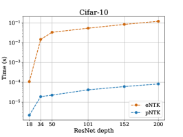
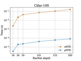
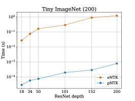
Figure 1: Wall-clock time to evaluate the eNTK and pNTK for one pair of inputs, across datasets and ResNet depths.

There has also been significant theoretical insight gained from empirical studies of networks’ NTKs. For instance, Fort et al. (2020) use NTKs to study how the loss geometry the NN evolves under gradient descent. Franceschi et al. (2022) employ NTKs to analyze the behaviour of Generative Adverserial Networks (GANs). Nguyen et al. (2021a, b) use NTKs for dataset distillation. He et al. (2020); Adlam et al. (2020) use NTKs to predict and analyze the uncertainty of a NN’s predictions. Tancik et al. (2020) use NTKs to analyze the behaviour of MLPs in learning high frequency functions, leading to new insights into our understanding of neural radiance fields. We thus believe NTKs will continue to be used in both theoretical and empirical deep learning.

Unfortunately, however, computing the NTK for practical networks is extremely challenging, and usually not computationally feasible. The “empirical” NTK (eNTK; we discuss the difference from what others term “the NTK” shortly) is

$$\Theta_{\theta}(x_{1},x_{2})=\left[J_{\theta}\left(f_{\theta}(x_{1})\right)\right]\left[J_{\theta}\left(f_{\theta}(x_{2})\right)\right]^{\top},$$ (1)

where $J_{\theta}\left(f_{\theta}(x)\right)$ denotes the Jacobian of the function $f$ at a point $x$ with respect to the flattened vector of all its parameters, $\theta\in\mathbb{R}^{P}$. If $D$ is the input dimension of $f$ and $O$ the number of outputs, we have $J_{\theta}\left(f_{\theta}(x)\right)\in\mathbb{R}^{O\times P}$ and $\Theta_{\theta}(x_{1},x_{2})\in\mathbb{R}^{O\times O}$. Thus, computing the eNTK between $N_{1}$ and $N_{2}$ data points yields $N_{1}N_{2}$ matrices, each of shape $O\times O$; we usually arrange this as an $N_{1}O\times N_{2}O$ matrix.

When computing an eNTK on tasks involving large datasets and with multiple output neurons, e.g. in a classification model with $O$ classes, the eNTK quickly becomes impractical regardless of how fast each entry is computed due to its $NO\times NO$ size. The full eNTK of a classification model even on the relatively small CIFAR-10 dataset (Krizhevsky, 2009), stored in double precision, takes over 1.8 terabytes in memory. For practical usage, we need something better.

This work presents a simple trick for a strong approximation of the eNTK that removes the $O^{2}$ from the size of the kernel matrix, resulting in a factor of $O^{2}$ improvement in the memory and up to $O^{3}$ in computation. Since for typical classification datasets $O$ is at least $10$ (e.g. CIFAR-10) and potentially $1{,}000$ or more (e.g. ImageNet, Deng et al., 2009), this provides multiple orders of magnitude savings over the full eNTK. We prove this approximation converges to the original eNTK at a rate of $\operatorname{\mathcal{O}}(n^{-1/2})$ for a standard-initialization NN of depth $L$ and width $n$ in each layer, and the predictions of kernel regression with the approximate kernel do the same. We also conduct diverse experimental investigations to support our theoretical results, across a range of architectures and settings. We hope this approximation further enables researches to employ NTKs towards theoretical and empirical advances in wide networks.

Infinite NTKs. In the infinite-width limit of appropriately initialized NNs, $\Theta_{\theta}$ converges almost surely at initialization to a particular kernel, and remains constant through training. Algorithms are available to compute this expectation exactly, but they tend to be substantially more expensive than computing (1) directly for all but extremely wide networks. The convergence to this infinite-width regime is slow in practice, and moreover it eliminates some of the interest of the framework: neural architecture search, predicting generalization of a pre-trained representation, and meta-learning are all considerably less interesting when we only consider infinite-width networks that do essentially no feature learning. Thus we focus here only on the “empirical” eNTK as in (1).

2 Related Work

Among the numerous recent works that have used eNTKs either to gain insights about various phenomenons in deep learning or to propose new algorithms, not many have publicized the computational costs and implementation details of computing eNTKs. Nevertheless, all are in agreement about the expense of such computations (Park et al., 2020; Holzmüller et al., 2023; Fort et al., 2020).

Several recent works have, mostly “quietly,” employed various techniques to avoid dealing with the full eNTK matrix; however, to the best of our knowledge, none provide any rigorous justifications. Wei et al. (2022, Section 2.3) point out that if the final layer of a NN is randomly initialized, the expected eNTK can be written as $K_{0}\otimes I_{O}$ for some kernel $K_{0}$, where $I_{O}$ is the $O\times O$ identity matrix and $\otimes$ is the Kronecker product. Thus, they use the approximation in which they only compute the eNTK with respect to one of the logits of the NN. Although their approach to approximating the eNTK is similar to ours, they don’t provide any rigorous bounds or empirical study of how closely the actual eNTK is approximated by its expectation in this regard. Wang et al. (2021) employs the same “single-logit” strategy, though they only mention the infinite-width limit as a motivation supporting their trick. Despite these claims, we will see in our experiments that the eNTK is generally not diagonal. We will, however, prove upper bounds on distance of our approximation to the eNTK, and provide experimental support that this approximation captures the behaviour of the eNTK even when the NN’s weights are not at initialization. Park et al. (2020) and Chen et al. (2021) also seem to use a form of “single-logit” approximation to eNTK, without explicitly mentioning it. Lee et al. (2019), by contrast, do use the full eNTK, and hence never compute the kernel on more than 256 datapoints.

Novak et al. (2022) recently performed an in-depth analysis of computational and memory complexity required for computing the eNTK, and proposed two new approaches (depending on the NN architecture) to reduce the time complexity, but not the memory burden, of computing the eNTK over explicitly implementing (1). Our approaches are complementary; in fact, we use their “structured derivatives” method to help compute our approximation.

3 Pseudo-NTK

We define the pseudo-NTK (pNTK), which we denote as $\hat{\Theta}_{\theta}(x_{1},x_{2})$, as

$$\underbrace{\left[\nabla_{\theta}\;\frac{1}{\sqrt{O}}\sum_{i=1}^{O}f^{(i)}_{\theta}(x_{1})\right]}_{1\times P}\underbrace{\left[\nabla_{\theta}\;\frac{1}{\sqrt{O}}\sum_{i=1}^{O}f^{(i)}_{\theta}(x_{2})\right]^{\top}}_{P\times 1},$$ (2)

where $f^{(i)}_{\theta}(x)$ denotes the $i$-th output of $f_{\theta}$ on the input $x$. While the eNTK is a matrix-valued kernel for each pair of inputs, the pNTK  is a traditional scalar-valued kernel.

Some recent work (Arora et al., 2019; Yang, 2020; Wei et al., 2022; Wang et al., 2021) has pointed out that in the infinite width limit $\lim_{n\to\infty}\Theta(x_{1},x_{2})$, the NTK becomes a constant-diagonal matrix, where the class-class component becomes identity. Thus, one can avoid computing the off-diagonal entries of the infinite-width NTK of each pair through using $\Theta_{\theta}(x_{1},x_{2})=\hat{\Theta}_{\theta}(x_{1},x_{2})\otimes I_{O}$, giving a drastic $\operatorname{\mathcal{O}}(O^{2})$ time and memory complexity decrease.

Practitioners have accordingly used the same approach in computing the eNTK of a finite width network, but with little to no further justification. We see in our experiments that for finite width networks, the NTK is not diagonal. In fact, we show that for most practical networks, it is very far from being diagonal, casting doubts on the validity of arguments justifying the approximation with asymptotic diagonality. We justify this category of approximation with theoretical bounds on the difference of the true NTK from the approximation (2), which we also call “sum of logits.”

Before our formal results and experimental evaluation, we give some intuition. First, suppose $f_{\theta}^{(i)}(x)=\phi(x)\cdot v_{i}$, so that $v_{i}{{}\in\mathbb{R}^{n_{L-1}}}$ is the $i$th row of a linear read-out layer; then $\frac{1}{\sqrt{O}}\sum_{i=1}^{O}f_{\theta}^{(i)}(x)=\phi(x)\cdot\left[\frac{1}{\sqrt{O}}\sum_{i=1}^{O}v_{i}\right]$. If the $v_{i}\sim\mathcal{N}(0,\sigma^{2}I_{n_{L-1}})$ are independent, $\frac{1}{\sqrt{O}}\sum_{i=1}^{O}v_{i}$ has the same normal distribution as, say, $v_{1}$. Thus, at initialization, our sum of logits approximation agrees in distribution with the first-logit approximation. Our proof uses the sum-of-logits form, though, and we believe it may be more sensible for networks that are not at random initialization.

Calling this vector (whether the first logit or sum of logits) $v$, we can think of (2) as the NTK of a model with a single scalar output as a function of $\phi$, whose last layer has weights $v$. When we linearize a network with that kernel for an $O$-class classification problem, getting the formula (5) discussed in Section 4.3, we end up effectively using a one-vs-rest classifier scheme. Thus, we can think of the pseudo-NTK as approximating the process of training $O$ one-vs-rest classifiers, rather than a single $O$-way classifier.

4 Approximation Quality of Pseudo-NTK

We will now study various aspects of the approximation of (2) to (1), both in theory and empirically. Our experiments compare different characteristics of pNTK and eNTK, both at initialization and throughout training. We evaluate four widely-used architectures: FCN (a fully-connected network of depth 3, as in Lee et al., 2019, 2020), ConvNet (a fully-convolutional network of depth 8, as in Arora et al., 2019, 2020; Lee et al., 2020), ResNet18 (He et al., 2016), and WideResNet-16-$k$ (Zagoruyko & Komodakis, 2016). We evaluate each architecture at different widths, as mentioned in the plot legends: we show exact widths for FCN, while for others we show a widening factor. For consistency with most other recent papers studying NTKs and properties of NNs in general, we focus on data from CIFAR-10 (Krizhevsky, 2009). Each experiment is repeated using three seedscolor=violet!20,noinline]Danica: Still true?; means and corresponding error bars are also shown, except when they interfered with clear interpretation of the plots. All models are trained for 200 epochs, using stochastic gradient descent (SGD), on 32GB NVIDIA V100 GPUs. More details on models and optimization are provided in Appendix A. The measured statistic for each experiment are reported after 0, 50, 100, 150, and 200 epochs.

A Note On Parameterization In order to be maximally applicable to practical implementations, both our experiments and our theoretical results are based on standard parameterization (“fan-in” variance). Although most related work uses the so-called NTK parameterization (“fan-out” variance), this is rarely used in practice while training NNs, mostly due to the poor generalization results achieved in comparison to training with standard parameterization (Park et al., 2019, Section I). We encountered similarly poor behaviour when training NNs with NTK parameterization, but note that our theorems could also be adapted to the fan-out case.

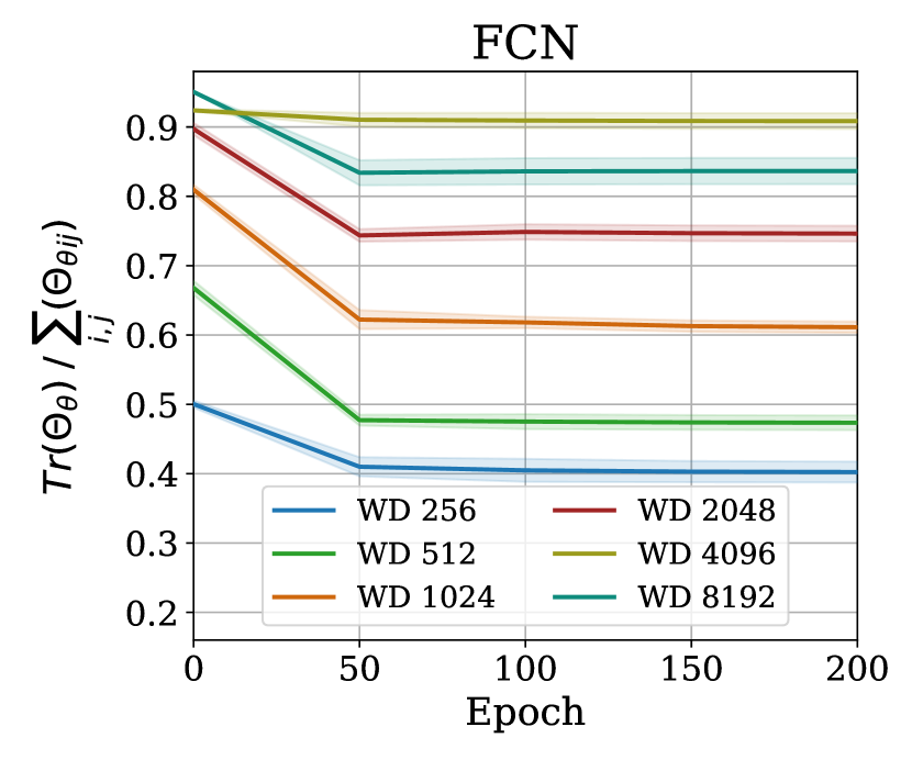
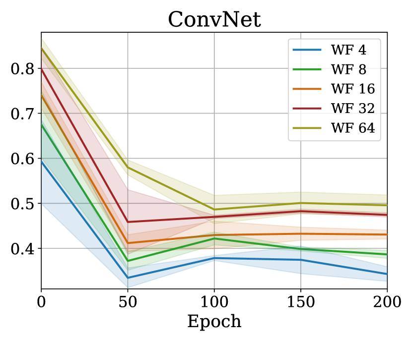
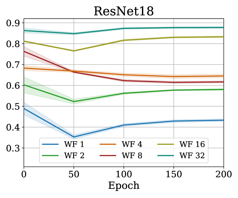
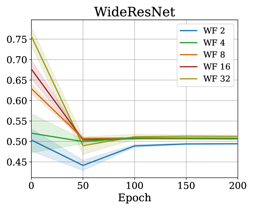
Figure 2: Comparing the magnitude of sum of on-diagonal and off-diagonal elements of $\Theta_{\theta}(\mathcal{D},\mathcal{D})$ at initialization and throughout training, based on $\mathcal{D}$ being $1000$ random points from CIFAR-10. The reported numbers are the average of $1000\times 1000$ matrices, each having a shape of $10\times 10$. The same subset has then been used to train the NN using SGD. As the NN’s width grows, the eNTK converges to being diagonal at initialization among all different architectures.

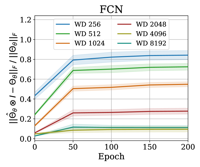
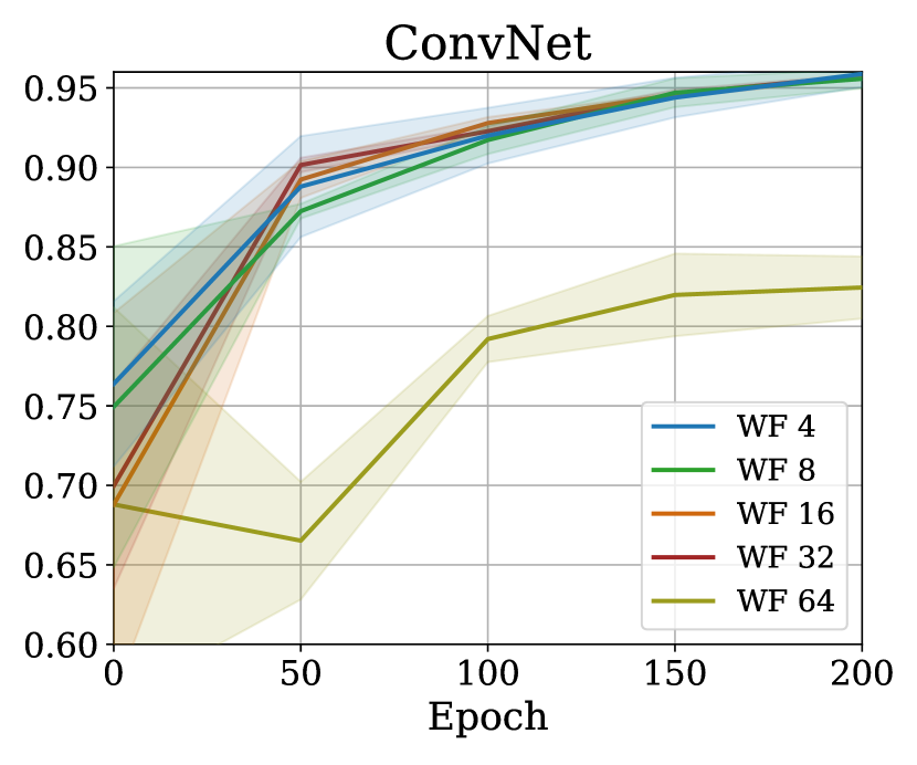
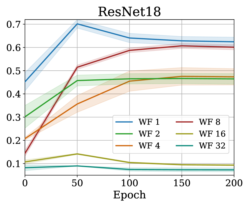
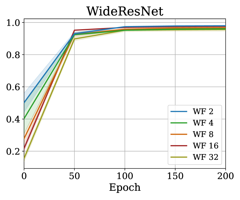
Figure 3: Evaluating the relative difference of Frobenius norm of $\Theta_{\theta}(\mathcal{D},\mathcal{D})$ and $\hat{\Theta}_{\theta}(\mathcal{D},\mathcal{D})\otimes I_{O}$ at initialization and throughout training, based on $\mathcal{D}$ being $1000$ random points from CIFAR-10. Wider nets have more similar $\lVert\Theta_{\theta}\rVert_{F}$ and $\lVert\hat{\Theta}_{\theta}\otimes I_{O}\rVert_{F}$ at initialization.

4.1 pNTK Converges to eNTK as Width Grows

The first crucial thing to verify is whether the pNTK kernel matrix approximates the true eNTK as a whole. We study this first in terms of Frobenius norm.

Theorem 4.1 (Informal).

Let $f_{\theta}:\mathbb{R}^{D}\to\mathbb{R}^{O}$ be a fully-connected network with layers of width $n$ whose parameters are initialized as in He et al. (2015), with ReLU-type activations. Let $\hat{\Theta}_{\theta}(x_{1},x_{2})$ be the pNTK of $f_{\theta}$ as in (2) and $\Theta_{\theta}(x_{1},x_{2})$ the eNTK as in (1) for a fixed pair of inputs $x_{1}$, $x_{2}$. With high probability over the initialization,

$$\frac{\lVert\hat{\Theta}_{\theta}(x_{1},x_{2})\otimes I_{O}-\Theta_{\theta}(x_{1},x_{2})\rVert_{F}}{\lVert\Theta_{\theta}(x_{1},x_{2})\rVert_{F}}\in\operatorname{\mathcal{O}}(n^{-\frac{1}{2}}).$$ (3)

Remark 4.2.

All of the results in the paper can be straightforwardly extended to networks with different widths, as long as the consecutive layers’ widths satisfy $n_{l+1}=\Theta(n_{l})$. Moreover, the results can be made architecturally universal with the techniques of Yang (2020); Yang & Littwin (2021).

Theorem 4.1 provides the first upper bound on the convergence rate of pNTK towards eNTK. A formal statement for Theorem 4.1 and its proof are in Appendix B.

Remark 4.3.

Based on the provided proof, it is straightforward that the ratio of information between off-diagonal and on-diagonal elements of the eNTK matrix converges to zero with a rate of $\operatorname{\mathcal{O}}(n^{-\frac{1}{2}})$ with high probability over random initialization, as depicted in Figure 2.

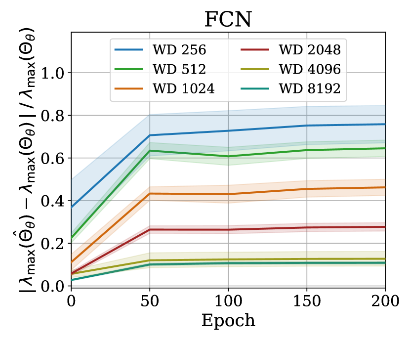
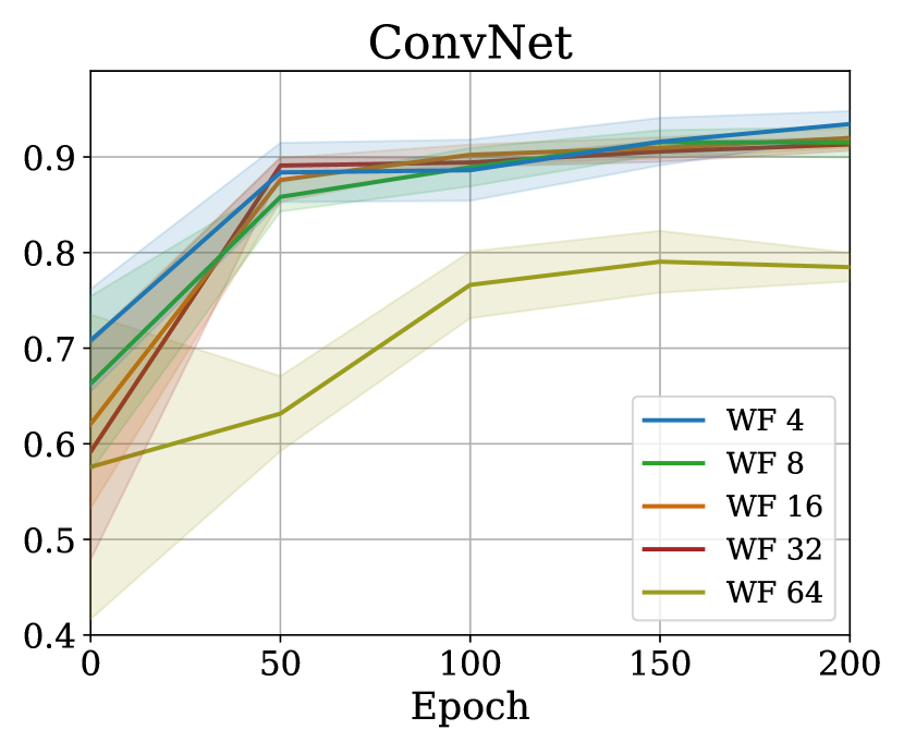
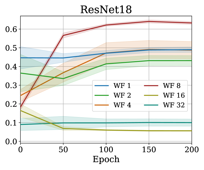
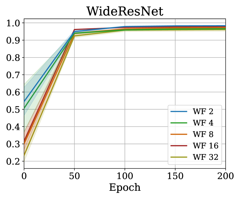
Figure 4: Evaluating the relative difference of $\lambda_{\max}$ of $\Theta_{\theta}(\mathcal{D},\mathcal{D})$ and $\hat{\Theta}_{\theta}(\mathcal{D},\mathcal{D})$ at initialization and throughout training, based on $\mathcal{D}$ being 1000 random points from CIFAR-10. Wider nets have more similar $\lambda_{\max}(\Theta_{\theta}(\mathcal{D},\mathcal{D}))$ and $\lambda_{\max}(\hat{\Theta}_{\theta}(\mathcal{D},\mathcal{D}))$.

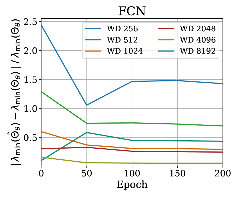
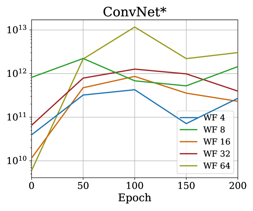
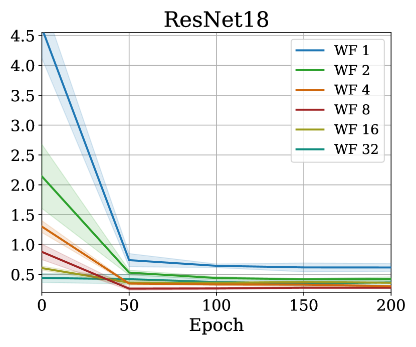
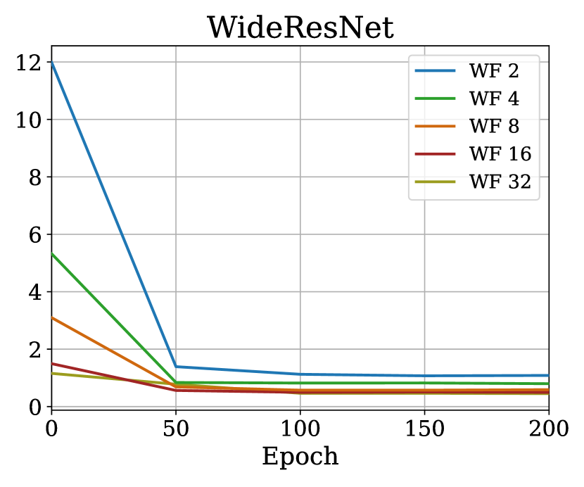
Figure 5: Evaluating the relative difference of $\lambda_{\min}$ of $\Theta_{\theta}(\mathcal{D},\mathcal{D})$ and $\hat{\Theta}_{\theta}(\mathcal{D},\mathcal{D})$ based on $\mathcal{D}$ being 1000 random points from CIFAR-10. Wider nets have more similar $\lambda_{\min}(\Theta_{\theta}(\mathcal{D},\mathcal{D}))$ and $\lambda_{\min}(\hat{\Theta}_{\theta}(\mathcal{D},\mathcal{D}))$. Note, though, the extremely large values reported for ConvNet; as observed by Lee et al. (2020) and Xiao et al. (2020), it is ill-conditioned and $\lambda_{\min}(\Theta_{\theta}(\mathcal{D},\mathcal{D}))\to 0$, while $\lambda_{\min}(\hat{\Theta}_{\theta}(\mathcal{D},\mathcal{D}))>0.001$, causing the huge discrepancy. More details in Appendix C.

Figure 2 shows that as the width grows, the sum of off-diagonal elements of $\Theta_{\theta}(x_{1},x_{2})$ becomes small compared to the diagonal. Furthermore, Figure 3 provides experimental support that as width grows, $\hat{\Theta}_{\theta}\otimes I_{O}$ converges to $\Theta_{\theta}$ in terms of relative Frobenius norm.

Theorem 4.1 only applies to epoch zero of these figures, as it assumes networks with weights at initialization. As can be seen in the figures, these results don’t necessarily apply to the NNs not at initialization (i.e., after a few epochs of training). This naturally gives rise to the question: Can the pNTK be used to analyze and represent NNs whose parameters are far from initialization? We will now take various experimental approaches towards studying this question.

4.2 Largest Eigenvalue Converges as Width Grows

As discussed before, the conditioning of a network’s eNTK has been shown to be closely related to generalization properties of the network, such as trainability and generalization risk (Xiao et al., 2018, 2020; Wei et al., 2022). Thus, we would like to know how well the pNTK’s eigenspectrum approximates that of the eNTK. The following theorem gives a bound on the rate of convergence between the maximum eigenvalues of the two kernels.

Theorem 4.4 (Informal).

Let $f_{\theta}:\mathbb{R}^{D}\to\mathbb{R}^{O}$ be a fully-connected network with layers of width $n$ whose parameters are initialized according to He et al. (2015) initialization, with ReLU-type activations. Let $\hat{\Theta}_{\theta}(x_{1},x_{2})$ be the corresponding pNTK of $f_{\theta}$ as in (2) and $\Theta_{\theta}(x_{1},x_{2})$ the corresponding eNTK as in (1) for a fixed pair of inputs $x_{1}$, $x_{2}$. With high probability over the initialization,

$$\frac{\lambda_{\max}(\hat{\Theta}_{\theta}(x_{1},x_{2})\otimes I_{O})-\lambda_{\max}\left(\Theta_{\theta}\left(x_{1},x_{2}\right)\right)}{\lambda_{\max}\left(\Theta_{\theta}\left(x_{1},x_{2}\right)\right)}\in\operatorname{\mathcal{O}}(n^{-\frac{1}{2}}).$$

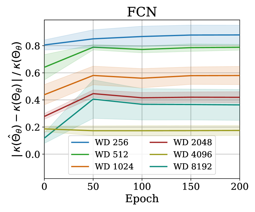
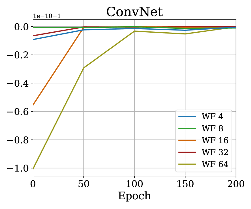
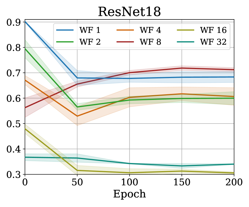
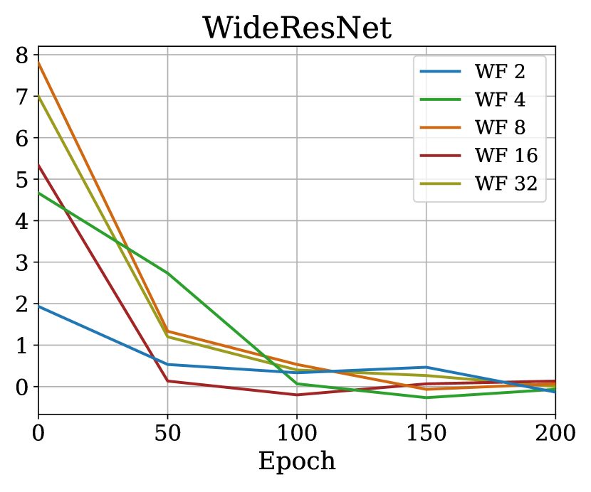
Figure 6: The relative difference in condition number, $\kappa(K)=\lambda_{\max}(K)/\lambda_{\min}(K)$, decreases for wider nets. The strange ConvNet plot is due to the issue in Figure 5; more details in Appendix C.

Theorem 4.4 bounds the difference between the maximum eigenvalue of pNTK and the maximum eigenvalue of eNTK based on the NN’s width, for networks at initialization. A formal statement for Theorem 4.4 and its proof are given in Appendix C. Figure 4 also supports this trend experimentally.

Figure 5 shows a similar trend for the minimum eigenvalues, although we have not found a proof of this convergence. This suggests that the condition number $\kappa=\lambda_{\max}/\lambda_{\min}$ should become similar as width grows; this is also supported by results in Figure 6.

Interestingly, the rate of increase/decrease in the difference between maximum and minimum eigenvalues and the condition numbers between pNTK and eNTK do not necessarily have a monotonic behaviour as the training goes on. Observing the exact values of $\lambda_{\min}$, $\lambda_{\max}$, and $\kappa$ for different architectures, widths at initialization and throughout training reveals that in ConvNet, WideResNet and ResNet18 architectures, $\lambda_{\min}$ is close to zero at initialization, but grows during training; the inverse phenomenon is observed with FCNs. Further investigations of these statistics might reveal interesting insights about the behaviour of NNs trained with SGD and the connections between eNTK and trainibility of the architecture.

4.3 Kernel Regression Using pNTK vs. eNTK

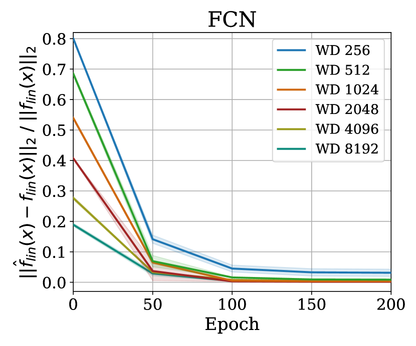
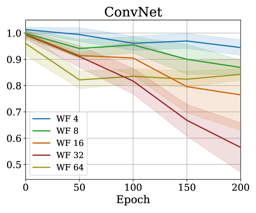
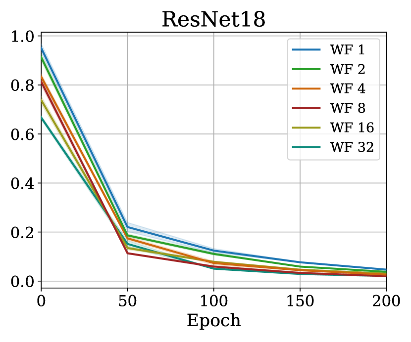
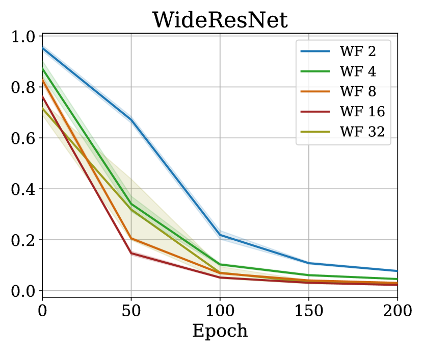
Figure 7: The relative difference of kernel regression outputs, (4) and (5), when training on $\lvert\mathcal{D}\rvert=1000$ random CIFAR-10 points and testing on $\lvert\mathcal{X}\rvert=500$. For wider NNs, the relative difference in $\hat{f}^{\mathit{lin}}(\mathcal{X})$ and $f^{\mathit{lin}}(\mathcal{X})$ decreases at initialization. Surprisingly, the difference between these two continues to quickly vanish while training the network.

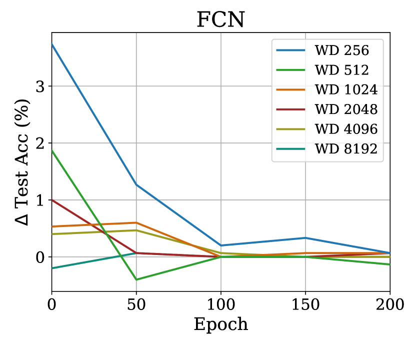
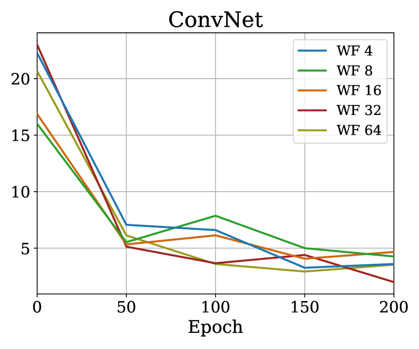
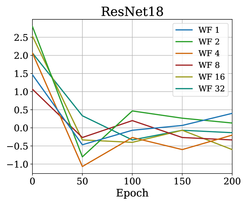
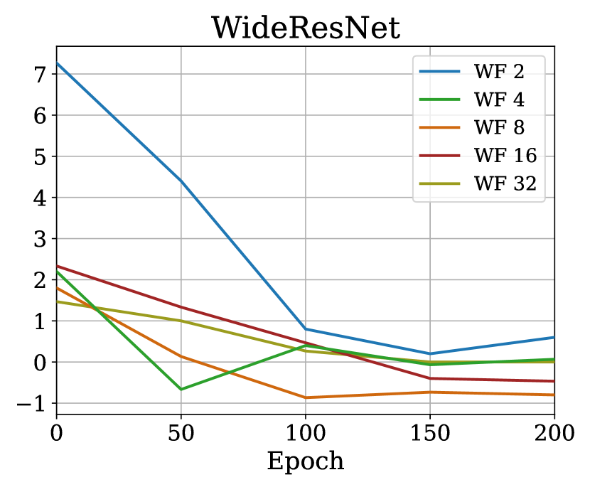
Figure 8: Using pNTK in kernel regression (as in Figure 7) almost always achieves a higher test accuracy than using eNTK. Wider NNs and trained nets have more similar prediction accuracies of $\hat{f}^{\mathit{lin}}$ and $f^{\mathit{lin}}$ at initialization. Again, the difference between these two continues to vanish throughout the training process using SGD.

Lee et al. (2019) proved that as a finite NN’s width grows, its training dynamics can be well approximated using the first-order Taylor expansion of that NN around its initialization (a linearized neural network). Informally, they showed that when $f$ is wide enough and trained on $\mathcal{D}$ with a suitably small learning rate, its predictions on $x$ can be approximated by those of the linearized network $f^{\mathit{lin}}$ given by

$$\underbrace{f_{0}(x)}_{O\times 1}+\underbrace{\Theta_{0}(x,\mathcal{D})}_{O\times NO}\;\underbrace{{\Theta_{0}(\mathcal{D},\mathcal{D})}^{-1}}_{NO\times NO}\,\underbrace{(\mathcal{Y}_{\mathcal{D}}-f_{0}(\mathcal{D}))}_{NO\times 1},$$ (4)

where $\mathcal{Y}_{\mathcal{D}}$ is the matrix of one-hot labels for the training points $\mathcal{D}$, and $\Theta_{0}$ is the eNTK of $f$ at initialization $f_{0}$. This is simply kernel regression on the training data $\mathcal{D}$ using the kernel $\Theta_{0}$ and prior mean $f_{0}$. Wei et al. (2022) use the same kernel in a generalized cross-validation estimator (Craven & Wahba, 1978) to predict the generalization risk of the NN. As discussed before, using the eNTK in these applications is practically infeasible, due to huge time and memory complexity of the kernel, but we show the pNTK approximates $f^{\mathit{lin}}(x)$ with much improved time and memory complexity.

Theorem 4.5 (Informal).

Let $f_{\theta}:\mathbb{R}^{D}\to\mathbb{R}^{O}$ be a fully-connected network with layers of width $n$ whose parameters are initialized as in He et al. (2015), with ReLU-type activations. Let $\hat{\Theta}_{\theta}(x_{1},x_{2})$ be the corresponding pNTK of $f_{\theta}$ as in (2) and $\Theta_{\theta}(x_{1},x_{2})$ the corresponding eNTK as in (1) for a fixed pair of inputs $x_{1}$, $x_{2}$. Define $\hat{f}^{\mathit{lin}}(x)$ as

$$\underbrace{f_{0}(x)}_{1\times O}+\underbrace{\hat{\Theta}_{\theta}(x,\mathcal{D})}_{1\times N}\,\underbrace{{\hat{\Theta}_{\theta}(\mathcal{D},\mathcal{D})}^{-1}}_{N\times N}\underbrace{(\mathcal{Y}_{\mathcal{D}}-f_{0}(\mathcal{D}))}_{N\times O}.$$ (5)

After proper reshaping, with high probability over random initialization,

$$\lVert\hat{f}^{\mathit{lin}}(x)-f^{\mathit{lin}}(x)\rVert_{F}\in\operatorname{\mathcal{O}}(n^{-\frac{1}{2}}).$$ (6)

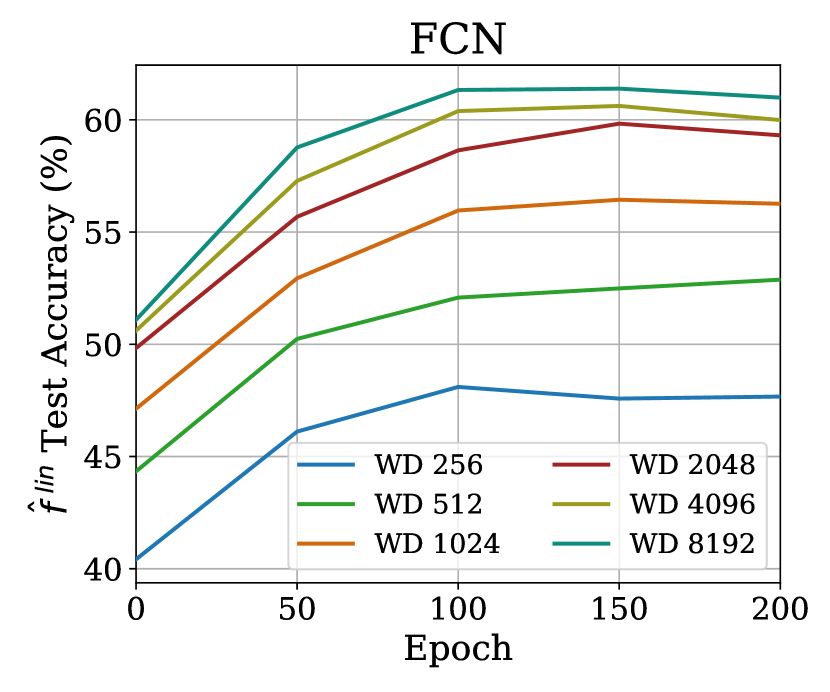
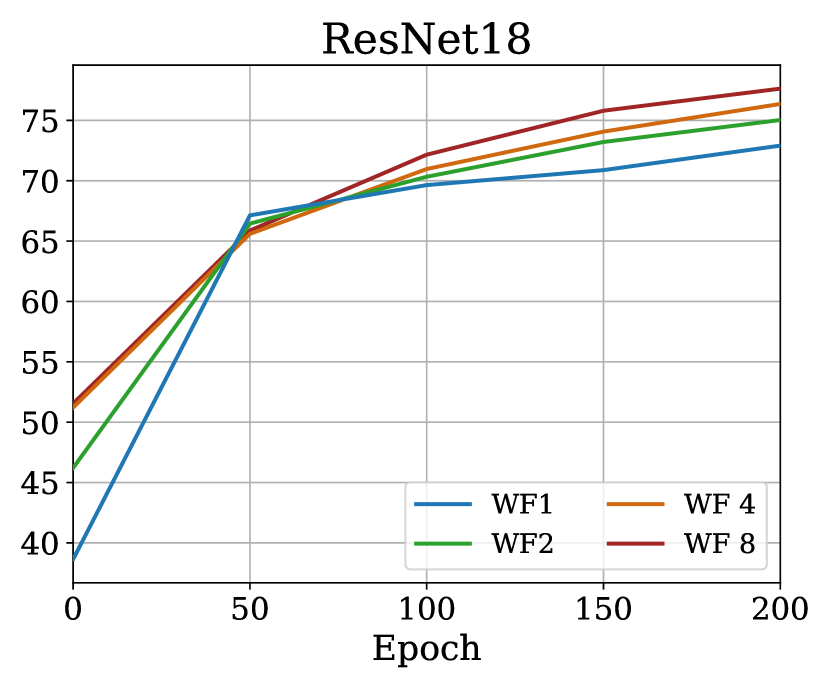
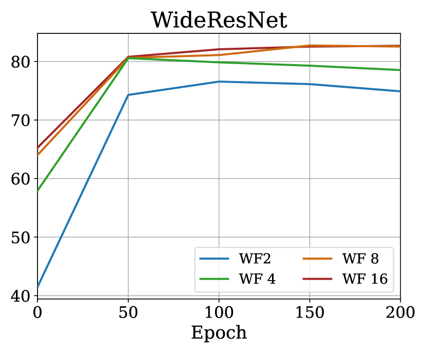
Figure 9: Evaluating the test accuracy of kernel regression predictions using pNTK as in (5) on the full CIFAR-10 dataset. As the NN’s width grows, the test accuracy of $\hat{f}^{\mathit{lin}}$ also improves, but eventually saturates with the growing width. Using trained weights in computation of pNTK results in improved test accuracy of $\hat{f}^{\mathit{lin}}$.

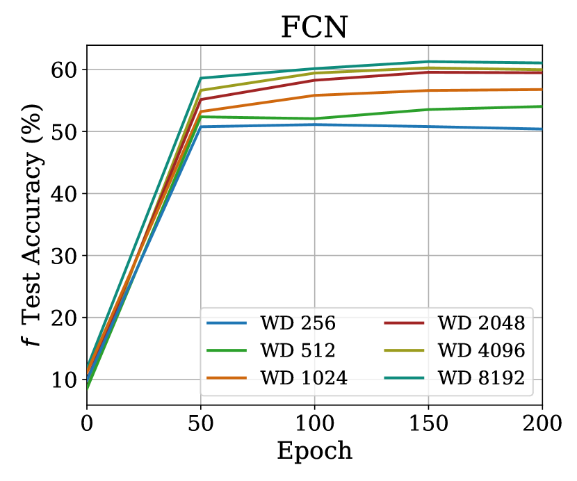
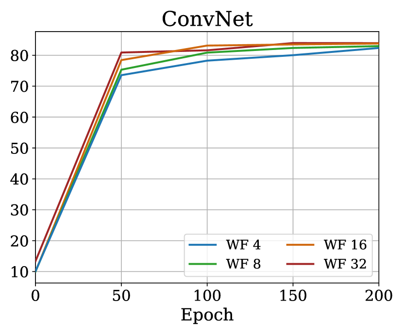
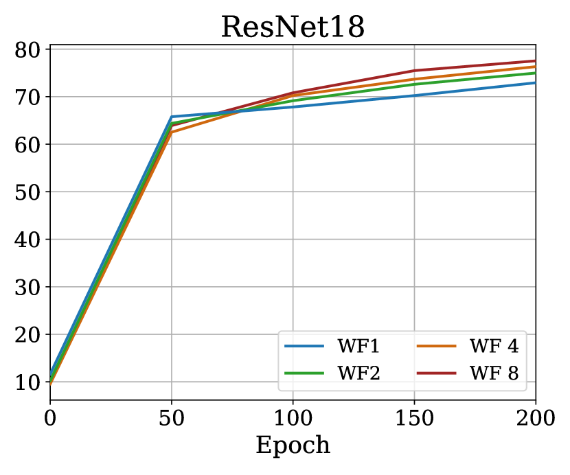
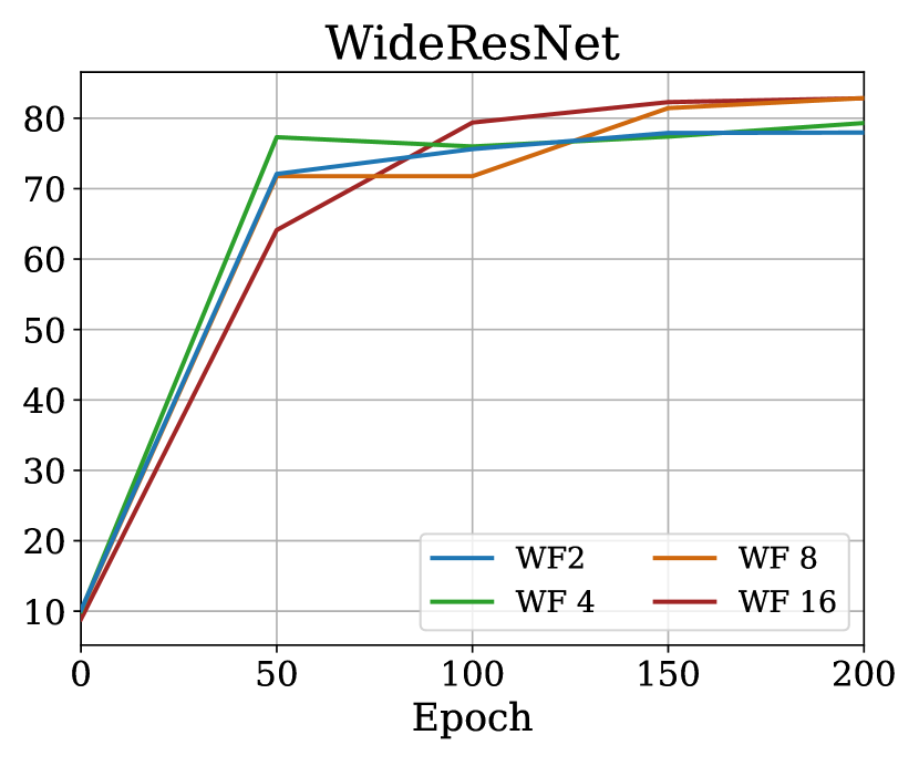
Figure 10: Evaluating the test accuracy of model $f$ throughout SGD training on the full CIFAR-10 dataset. In contrast to $\hat{f}^{\mathit{lin}}$, the test accuracy of $f$ does not significantly improve with growing width.

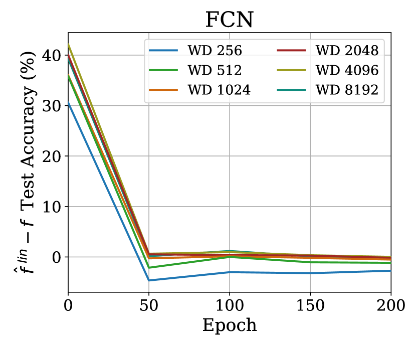
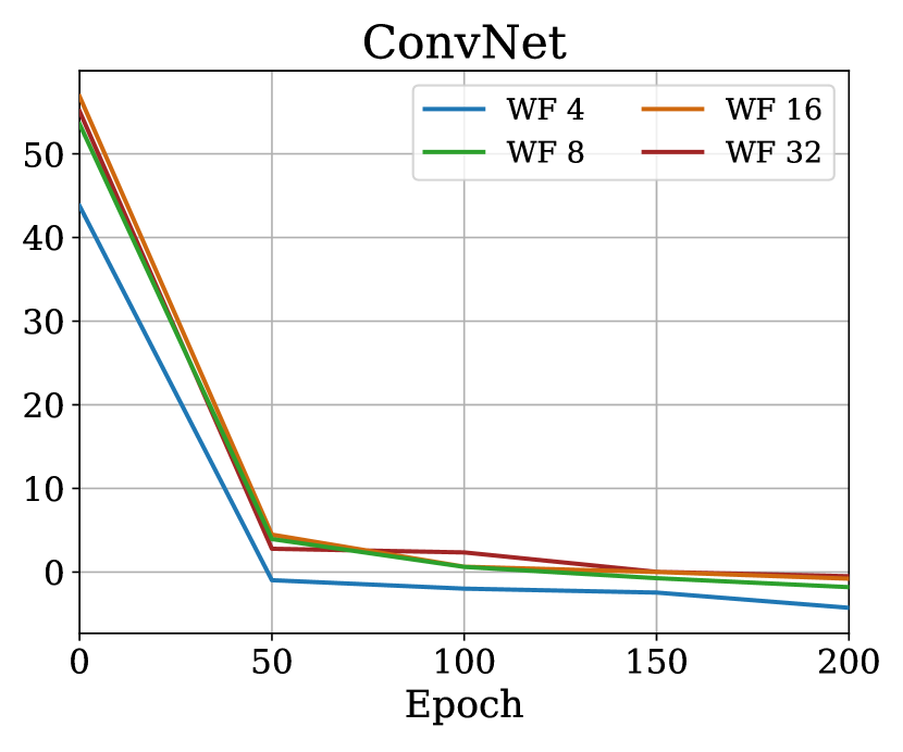
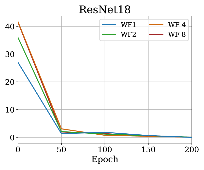
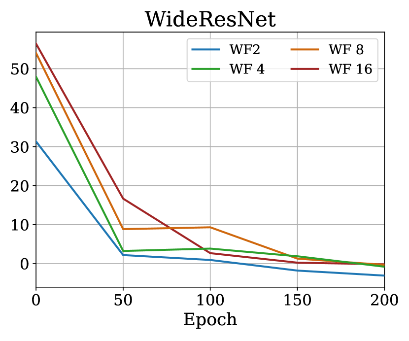
Figure 11: Evaluating the difference in test accuracy of kernel regression using pNTK as in (5) vs the current model $f$ throughout SGD training on the full CIFAR-10 dataset: how much does a linearized predictor with the current representation improve prediction accuracy over the current model obtained by SGD?

A formal statement is given and proved in Appendix D.

Figure 7 also supports that as width grows, the predictions of kernel regression using $\hat{\Theta}_{\theta}$ converge to the prediction of those obtained from using $\Theta_{\theta}$, while requiring orders of magnitude of less memory and time to compute. Figure 8 shows similar results for the difference in prediction accuracies achieved using kernel regression through $\hat{\Theta}_{\theta}$ and $\Theta_{\theta}$ kernels. Appendix D also shows further analysis of how well the linearized network predicts the final accuracy of the trained model for each architecture and width pair. Although $\lVert\hat{f}^{\mathit{lin}}(x)-f^{\mathit{lin}}(x)\rVert_{F}$ decreases with width of the network in Figure 7 at initialization, this does not necessarily translate to a monotonic behaviour in prediction accuracies, a non-smooth function of the vector of predictions; we do see that the expected pattern more or less holds, however.

A surprising outcome depicted in Figures 7 and 8 is that while training the model’s parameters, predictions of $\hat{f}^{\mathit{lin}}$ and $f^{\mathit{lin}}$ converge very quickly. This is particularly intriguing, as it contrasts the results depicted in Figures 2, 3, 4 and 6. In other words, although the kernels $\Theta_{\theta}$ and $\hat{\Theta}_{\theta}\otimes I_{O}$ seem to be diverging in Frobenius norm, eigenspectrum, and so on, kernel regression using those two kernels converges quickly, so that after 50 epochs the difference in predictions almost totally vanishes. We believe further investigation of why this phenomenon is observed could lead to new interesting insights about the training dynamics of NNs.

5 Application: Full Regression on CIFAR-10

Thanks to the reduction in time and memory complexity of pNTK over eNTK, motivated by Theorem 4.5 and experimental findings in Figure 8, we finally evaluate the corresponding pNTKs of the four architectures that we have used in our experimental evaluations in different widths using full CIFAR-10 data, at initialization and throughout training the models under SGD. As mentioned previously, running kernel regression with eNTK on all of CIFAR-10 would require evaluating $25\times 10^{10}$ Jacobian-vector products and more than $\approx 1.8$ terabytes of memory; using pNTK, this can be done with a far more reasonable $25\times 10^{8}$ Jacobian-vector products and $\approx 18$ gigabytes of memory. This is still a heavy load compared to, say, direct SGD training, but is within the reach of standard compute nodes.

Figure 9 shows the test accuracy of $\hat{f}^{\mathit{lin}}$ on the full train and test sets of CIFAR-10. In the infinite-width limit, the test accuracy of $\hat{f}^{\mathit{lin}}$ at initialization (and later, because the kernel stays constant in this regime) should match the final test accuracy of $f$: that is, the epoch 0 points in Figure 9 would agree with roughly the epoch 200 points in Figure 10. This comparison is plotted directly in Appendix F. Furthermore, the test accuracies of predictions of kernel regression using the pNTK are lower than those achieved by the NTKs of infinite-width counterparts for fully-connected and fully-convolution networks. This is consistent with results on eNTK by Arora et al. (2019) and Lee et al. (2020), although Arora et al. (2019) studied only a “CIFAR-2” version.

It is worth noting from Figures 9 and 11 that, in contrast to the findings of Fort et al. (2020), we observe that the corresponding pNTK of the NN continues to change even after epoch 50 of SGD training. Although for fully-connected networks and some versions of ResNet18, this change is not significant, in fully-convolutional networks and WideResNets, the pNTK continues to exhibit changes until epoch 150, where the training error has vanished. We remark that Fort et al. (2020) analyzed eNTKs based on only 500 random samples from CIFAR-10, while the pNTK approximation has enabled us to run our analysis on the $100$-times larger full dataset.

Lastly, to help the community better analyze the properties of NNs and their training dynamics, and avoid wasting computation by redoing this work, we plan to share computed pNTKs for all the mentioned architectures and widths, as well as ResNets with 34, 50, 101 and 152 layers on CIFAR-10 and CIFAR-100 (Xiao et al., 2017) datasets, both at initialization and using pretrained ImageNet (Deng et al., 2009) weights. We hope that our contribution will enable further analyses and breakthroughs towards a stronger theoretical understanding of the training dynamics of deep NNs.

Figure 12: Comparison of pNTK with eNTK on a look-ahead active learning task. pNTK is much faster than eNTK without losing performance.

6 Application: Active Learning

One use case for eNTK is in active learning, where the model requests annotations for specific data points in an “active” manner. Recently, Mohamadi et al. (2022) used kernel regression with the pNTK to approximate a re-trained model for the computation of “look-ahead” data acquisition functions in active learning. That is, a model requests annotations for data points where training on them is likely to make the model’s output on test data change the most. In Figure 12, we compare the performance of their scheme using pNTK (as they did in their work) to using the full eNTK, in terms of both active learning performance on the MNIST dataset (left axis), and wall-clock time needed to compute the acquisition function (right axis). Similarly to that work, we measure accuracy on the test set for a model which begins with $100$ randomly trained points, then acquires $20$ additional labelled points in each cycle. The acquisition performance with the pNTK matches that with the eNTK, but computation is much faster, taking about 15% as long in total on this problem with $O=10$. Active learning performance is measured in accuracy on the test set using a model trained on a labelled set.

7 Discussion

Our pNTK approach to approximating the eNTK has provable bounds, good empirical performance, and multiple orders of magnitude improvement in runtime speed and memory requirements over the direct eNTK. We evaluate our claims and the quality of the approximation under diverse settings, giving new insights into the behaviour of the eNTK with trained representations. We help justify the correctness of recent approximation schemes, and hope that our rigorous results and thorough experimentation will help researchers develop a deeper understanding of the training dynamics of finite networks, and develop new practical applications of the NTK theory.

One major remaining question is to theoretically analyze what happens to the pNTK or eNTK during SGD training of the network. In particular, the fast convergence of $\hat{f}^{\mathit{lin}}$ and $f^{\mathit{lin}}$ when training the network, as seen in Figures 8 and 7, runs counter to our expectations based on the approximation worsening in Frobenius norm (Figure 7), maximum eigenvalue (Figure 4), and condition number (Figure 6). This seems likely to be important to practical use of the pNTK.

Perhaps relatedly, it is also unclear why pNTK consistently results in higher prediction accuracies than when kernel regression is done using eNTK, given that our motivation for pNTK is entirely in terms of approximating the eNTK (Figure 8). Intuitively, this may be related to a regularization-type effect: the pNTK corresponds to a particularly limited choice of a “separable” operator-valued kernel (see, e.g., Álvarez et al., 2012). Separable kernels are a common choice in that literature for both computational and regularization reasons; by enforcing this particularly simple form, we remove many degrees of freedom relating to the interaction between “tasks” (different classes) that may be unnecessary or hard to estimate accurately with the eNTK. This might, in some sense, correspond to a one-vs-one rather than one-vs-rest framework in the intuitive sense discussed in Section 3. Understanding this question in more detail might require a more detailed understanding of the structure of the eNTK at finite width, and/or a much more detailed understanding of the interaction between classes in the dataset with learning in the NTK regime. Finally, even the pNTK is still rather expensive compared to running SGD on neural networks. It might make for a better starting point than the full eNTK for other speedup methods, however, like kernel approximation or advanced linear algebra solvers (e.g. Rudi et al., 2017).

Appendix A Details of Experimental Setup

In this section, we present the details on the experimental setup used for the plots depicted in the main body of the paper. As mentioned, the exact width for FCNs have been reported. For WideResNet-16-k we use two block layers, and the initial convolution in the network has a width of $16\mathrm{WF}$ where $\mathrm{WF}$ is the reported $\mathrm{WF}$. For instance, $\mathrm{WF}=16$ means that the first block layer has a width of 256 and the second block layer has a width of 512. For ResNet18, we also used the same approach, multiplying $\mathrm{WF}$ by 16. Thus, when $\mathrm{WF}=4$, the constructed network will have the exact architecture as the classical ResNet18 architecture reported. A $\mathrm{WF}$ of 16 means a ResNet18 with each layer being 4 times wider than the original width.

When training the neural networks using SGD, a constant batch size of 128 was used across all different networks and different dataset sizes used for training. The learning rate for all networks was also fixed to 0.1. However, not all networks were trainable with this fixed learning rate, as the gradients would sometimes blow up and give NaN training loss, typically for the largest width of each mentioned architecture. In those cases, we decreased the learning rate to 0.01 to train the networks.

Note that to be consistent with the literature on NTKs, techniques like data augmentation have been turned off, but a weight decay of 0.0001 along with a momentum of 0.9 for SGD is used. Data augmentation here plays an important role in the attained test accuracies of the fully trained networks.

Appendix B Relative Convergence of Kernel Matrices

This section will prove Theorem 4.1, in two parts. First, we give a generic analysis in Section B.1 bounding the difference between the $pNTK$ and $eNTK$ for any network whose last layer is linear and random, in terms of the norm of the eNTK of the previous parts of the network. Section B.3 then bounds the growth of the eNTK for “fan-in” ReLU networks; their combination gives a $\operatorname{\mathcal{O}}_{p}(1/\sqrt{n})$ bound on the Frobenius difference between the eNTK and pNTK for width-$n$ fan-in ReLU nets. Later subsections apply these results to various applications.

B.1 Linear Read-Out Layers

Towards this, we first define some notation and show a simple recursive formula for computing the tangent kernel that we take advantage of to prove the theorems. Consider a NN $f:\mathbb{R}^{D}\to\mathbb{R}^{O}$. We assume the final read-out layer of the NN $f$ is a dense layer with width $n$. Assuming the NN $f$ has $L$ layers, we define $\theta_{l}$ to be the corresponding parameters of layer $l\in\{1,2,\dots,L\}$. Furthermore, let’s define $g:{\color[rgb]{0,0,0}\mathbb{R}^{D}}\to\mathbb{R}^{n}$ as the output of the penultimate layer of the NN $f$, such that $f(x)=\theta_{L}g(x)$ for some $\theta_{L}\in\mathbb{R}^{O\times w}$.

As noted by Lee et al. (2019) and Yang (2020), the NTK can be reformulated as the layer-wise sum of gradients (when the parameters of each layer $\theta_{l}$ are assumed to be vectorized) of the output with respect to $\theta_{l}$. Accordingly, we denote the eNTK of a NN $f$ as

$$\Theta_{f}(x_{1},x_{2})=\sum_{l=1}^{L}\nabla_{\theta_{l}}f(x_{1}){\nabla_{\theta_{l}}f(x_{2})}^{\top}.$$ (7)

Now, noting that as the final layer of $f$ is a dense layer, we can use the chain rule to write $\nabla_{\theta_{l}}f(x)$ as $\frac{\partial f}{\partial g(x)}\frac{\partial g(x)}{\partial\theta_{l}}$ where $\frac{\partial f(x)}{\partial g(x)}=\theta_{L}$. Thus, we can rewrite (7) as

$$\begin{split}\Theta_{f}(x_{1},x_{2})&=\sum_{l=1}^{L-1}\theta_{L}\nabla_{\theta_{l}}g(x_{1})\,{\nabla_{\theta_{l}}g(x_{2})}^{\top}{\theta_{L}}^{\top}+\nabla_{\theta_{L}}f(x_{1}){\nabla_{\theta_{L}}f(x_{2})}^{\top}\\ &=\theta_{L}\left(\sum_{l=1}^{L}\nabla_{\theta_{l}}g(x_{1})\,\nabla_{\theta_{l}}g(x_{2})^{\top}\right){\theta_{L}}^{\top}+{g(x_{1})}^{\top}g(x_{2})\,I_{O}\\ &=\theta_{L}\,\Theta_{g}(x_{1},x_{2})\,{\theta_{L}}^{\top}+{g(x_{1})}^{\top}g(x_{2})\,I_{O}.\end{split}$$ (8)

Recall that we can view the pNTK of a network $f$ as simply adding a fixed, non-trainable dense layer to the network with weights $v$, where $v$ is either a standard basis vector for the single-logit approximation, or $\frac{1}{\sqrt{O}}\mathbf{1}_{O}$ for the sum-of-logits form. Then (8) shows us that the pNTK is simply a weighted sum of the eNTK’s elements,

$$\hat{\Theta}_{f}(x_{1},x_{2})=v^{\mathsf{T}}\Theta_{f}(x_{1},x_{2})v;$$ (9)

note that the second term does not appear since $v$ is not a trainable parameter.

The key result of this subsection, which holds fairly generally, is based on showing that, when $\theta_{L}$ is at initialization, off-diagonal entries of $\theta_{L}\Theta_{g}\theta_{L}^{\mathsf{T}}$ are near the pNTK’s corresponding value of zero, while diagonal entries are close to $\Theta_{f}$. Specifically, we have the following result for the single-logit approximation, i.e. when $v$ in (9) is one-hot.

Lemma B.1.

Let $f$ be of the form $f(x)=Wg(x)$, where $W\in\mathbb{R}^{O\times n}$ and $g$ is an arbitrary deep network. Suppose that $W$ has independent, zero-mean, sub-gaussian entries with variance parameter $\nu$. Let $\delta>0$ be smaller than a constant depending only on $O$. Let $x_{1}$, $x_{2}$ be arbitrary input points. Then, with high probability over the random value of $W$,

$$\lVert\Theta_{f}(x_{1},x_{2})-\hat{\Theta}_{f}(x_{1},x_{2})I_{O}\rVert_{F}\leq\operatorname{\mathcal{O}}_{p}\left(\nu\lVert\Theta_{g}(x_{1},x_{2})\rVert_{F}\right).$$ (10)

For standard He et al. (2015) initialization, $\nu=\frac{1}{n}$. We will later show that for standard ReLU networks of width $n$ at initialization, $\lVert\Theta_{g}(x_{1},x_{2})\rVert_{F}=\operatorname{\mathcal{O}}_{p}(\sqrt{n})$, implying that the difference between the pNTK and the eNTK is $\operatorname{\mathcal{O}}_{p}(1/\sqrt{n})$.

For Gaussian weights $W$, the same guarantees follow for the sum-of-logits approximation ($v=\frac{1}{\sqrt{O}}\mathbf{1}_{O}$) by noting that for fixed $g$ and random $W$, the joint distribution of $f(x)$ and $\hat{f}(x)=v^{\mathsf{T}}f(x)$ are identical for any unit-norm $v$.

Our proof is based on the following key tool.

Proposition B.2 (Hanson-Wright Inequality; Vershynin 2018, Theorem 6.2.1).

Let $x$ be a random vector with independent centered sub-gaussian entries with variance proxy $\nu$, and let $A$ be a square matrix. Let $c>0$ be a universal constant. Then

$$\Pr\Big{(}\big{|}x^{\mathsf{T}}Ax-\operatorname*{\mathbb{E}}[x^{\mathsf{T}}Ax]\big{|}\geq t\Big{)}\leq 2\exp\left(-c\min\left(\frac{t^{2}}{\nu^{2}\lVert A\rVert_{F}^{2}},\frac{t}{\nu\lVert A\rVert}\right)\right).$$

(A version with explicit constants, but in a slightly less convenient form, is given by Epperly 2022.)

The following form converts to an error probability of $\delta$, and gives a slightly simpler but weaker bound using $\lVert A\rVert\leq\lVert A\rVert_{F}$.

Corollary B.3.

In the setup of Proposition B.2, it holds with probability at least $1-\delta$ that

$$\lvert x^{\mathsf{T}}Ax-\operatorname*{\mathbb{E}}[x^{\mathsf{T}}Ax]\rvert\leq\nu\lVert A\rVert_{F}\max\left(\tfrac{1}{c}\log\tfrac{2}{\delta},\sqrt{\tfrac{1}{c}\log\tfrac{2}{\delta}}\right).$$

Corollary B.4.

Let $x$ and $y$ be independent random vectors, whose entries are independent, centered, and sub-gaussian with variance proxy $\nu$. Let $A$ be any square matrix, and $c>0$ the universal constant of Proposition B.2. Then

$$\Pr\left(\lvert x^{\mathsf{T}}Ay\rvert\geq t\right)\leq 2\exp\left(-2c\min\left(\frac{t^{2}}{\nu^{2}\lVert A\rVert_{F}^{2}},\frac{t}{\nu\lVert A\rVert}\right)\right).$$

This implies that with probability at least $1-\delta$, we have that

$$\lvert x^{\mathsf{T}}Ax-\operatorname*{\mathbb{E}}[x^{\mathsf{T}}Ax]\rvert\leq\nu\lVert A\rVert_{F}\max\left(\tfrac{1}{2c}\log\tfrac{2}{\delta},\sqrt{\tfrac{1}{2c}\log\tfrac{2}{\delta}}\right).$$

Proof.

Notice that

$$\begin{bmatrix}x\\ y\end{bmatrix}^{\mathsf{T}}\underbrace{\begin{bmatrix}0&\tfrac{1}{2}A\\ \tfrac{1}{2}A^{\mathsf{T}}&0\end{bmatrix}}_{\tilde{A}}\begin{bmatrix}x\\ y\end{bmatrix}=\tfrac{1}{2}x^{\mathsf{T}}Ay+\tfrac{1}{2}y^{\mathsf{T}}A^{\mathsf{T}}x=x^{\mathsf{T}}Ay.$$ (11)

The vector $\begin{bmatrix}x\\ y\end{bmatrix}$ satisfies the conditions for Proposition B.2. We have $\lVert\tilde{A}\rVert_{F}=\sqrt{\tfrac{1}{4}+\tfrac{1}{4}}\,\lVert A\rVert_{F}=\frac{1}{\sqrt{2}}\lVert A\rVert_{F}$, while

$$\lVert\tilde{A}\rVert=\sup_{\lVert x\rVert^{2}+\lVert y\rVert^{2}=1}\sqrt{\lVert\tfrac{1}{2}Ay\rVert^{2}+\lVert\tfrac{1}{2}A^{\mathsf{T}}x\rVert^{2}}=\tfrac{1}{2}\lVert A\rVert\sup_{\lVert x\rVert^{2}+\lVert y\rVert^{2}=1}\sqrt{\lVert x\rVert^{2}+\lVert y\rVert^{2}}=\tfrac{1}{2}\lVert A\rVert.$$

Noting that $\operatorname*{\mathbb{E}}x^{\mathsf{T}}Ay=0$, the proof follows by applying Propositions B.2 and B.3 to (11). ∎

We are now ready to prove the previous result.

Proof of Lemma B.1.

Assume without loss of generality that $\hat{\Theta}_{f}$ uses the first-logit approximation, i.e. $v=(1,0,\dots,0)$. Also assume $O>1$, since for $O=1$ the eNTK and pNTK are trivially identical.

Define the difference matrix between the two kernels as, recalling (8) and (9),

$$D(x_{1},x_{2}) =\Theta_{f}(x_{1},x_{2})-\hat{\Theta}_{f}(x_{1},x_{2})I_{O}$$

$$=\left[W\Theta_{g}(x_{1},x_{2})W^{\mathsf{T}}+g(x_{1})^{\mathsf{T}}g(x_{2})I_{O}\right]-v^{\mathsf{T}}\left[W\Theta_{g}(x_{1},x_{2})W-g(x_{1})^{\mathsf{T}}g(x_{2})\right]vI_{O}$$

$$=W\Theta_{g}(x_{1},x_{2})W^{\mathsf{T}}-W_{1}^{\mathsf{T}}\Theta_{g}(x_{1},x_{2})W_{1}I_{O}.$$

We will use the Hanson-Wright inequality (Propositions B.2, B.3 and B.4) to bound each entry of this matrix with high probability, then use a union bound to bound the overall Frobenius norm of $D(x_{1},x_{2})$.

We begin by bounding the off-diagonal elements of $D$. By (8) and (9), we can see that for any $i\neq j$, $D_{ij}(x_{1},x_{2})=W_{i}^{\mathsf{T}}\Theta^{(L-1)}W_{j}$. Because the matrix $D$ is symmetric, there are $\frac{O(O-1)}{2}$ distinct off-diagonal entries to bound. Using a union bound with Corollary B.4, we obtain that for any $\delta<2O(O-1)e^{-2c}$, it holds with probability at least $1-\delta/2$ that

$$\forall i\neq j,\quad|D_{ij}(x_{1},x_{2})|\leq\nu\lVert\Theta_{g}(x_{1},x_{2})\rVert_{F}\frac{1}{2c}\log\dfrac{2O(O-1)}{\delta}.$$ (12)

$D_{11}(x_{1},x_{2})$ is identically zero. For the other diagonal elements, we have that

$$\begin{split}D_{ii}(x_{1},x_{2})&=W_{i}^{\top}\Theta^{(L-1)}W_{i}-W_{1}^{\top}\Theta_{g}W_{1}\\ &=(W_{i}-W_{1})^{\top}\Theta^{(L-1)}(W_{i}+W_{1})\underbrace{{}-W_{i}^{\top}\Theta_{g}W_{1}+W_{1}^{\top}\Theta_{g}W_{i}}_{\;=0\text{, as }\Theta_{g}\text{ is symmetric}}\\ &=\begin{bmatrix}W_{i}\\ W_{1}\end{bmatrix}^{\top}\underbrace{\Bigg{(}\begin{bmatrix}I_{n}\\ -I_{n}\end{bmatrix}\Theta_{g}\begin{bmatrix}I_{n}&I_{n}\end{bmatrix}\Bigg{)}}_{\Theta_{g}^{*}}\begin{bmatrix}W_{i}\\ W_{1}\end{bmatrix}.\end{split}$$ (13)

Noting that $\Theta_{g}^{*}=\begin{bmatrix}\Theta_{g}&\Theta_{g}\\ -\Theta_{g}&-\Theta_{g}\end{bmatrix}$, we have that $\lVert\Theta_{g}^{*}\rVert_{F}=2\lVert\Theta_{g}\rVert_{F}$. Thus, applying Corollary B.3 to each of the $O-1$ entries and taking a union bound, we find that as long as $\delta<4(O-1)e^{-c}$, it holds with probability at least $1-\delta/2$ that

$$\forall i,\quad\big{|}D_{ii}(x_{1},x_{2})\big{|}\leq 2\nu\lVert\Theta_{g}(x_{1},x_{2})\rVert_{F}\frac{1}{c}\log\dfrac{4(O-1)}{\delta}.$$ (14)

Combining (12) and (14), we obtain that as long as $\delta<2(O-1)e^{-c}\min(Oe^{-c},2)$,

$$\lVert D(x_{1},x_{2})\rVert_{F}\leq\nu\lVert\Theta_{g}(x_{1},x_{2})\rVert_{F}\frac{1}{c}\sqrt{O(O-1)\left(\tfrac{1}{2}\log\frac{2O(O-1)}{\delta}\right)^{2}+(O-1)\left(2\log\frac{4(O-1)}{\delta}\right)^{2}}.\qed$$

B.2 Background on sub-exponential variables

The following proofs rely heavily on concentration inequalities for sub-exponential random variables; we will first review some background on these quantities.

A real-valued random variable $X$ with mean $\mu$ is called sub-exponential (see e.g. Wainwright, 2019) if there are non-negative parameters $(\nu,\alpha)$ such that

$$\operatorname*{\mathbb{E}}[e^{\lambda(X-\mu)}]\leq e^{\frac{\nu^{2}\lambda^{2}}{2}}\quad\text{ for all }\lvert\lambda\rvert<\frac{1}{\alpha}.$$

We use $X\sim SE(\nu,\alpha)$ to denote that $X$ is a sub-exponential random variable with parameters $(\nu,\alpha)$, but note that this is not a particular distribution.

One famous sub-exponential random variable is the product of the absolute value of two standard normal distributions, $z_{i}\sim\mathcal{N}(0,1)$, such that the two factors are either independent ($X_{1}=\lvert z_{1}\rvert\lvert z_{2}\rvert\sim SE(\nu_{p},\alpha_{p})$ with mean $2/\pi$) or the same ($X_{2}=z^{2}\sim SE(2,4)$ with mean 1). We now present a few lemmas regarding sub-exponential random variables that will come in handy in the later subsections of the appendix.

Lemma B.5.

If a random variable $X$ is sub-exponential with parameters $(\nu,\alpha)$, then the random variable $sX$ where $s\in\mathbb{R}^{+}$ is also sub-exponential with parameters $(s\nu,s\alpha)$.

Proof.

Consider $X\sim SE(\nu,\alpha)$ and $X^{\prime}=sX$ with $\operatorname*{\mathbb{E}}[X^{\prime}]=s\operatorname*{\mathbb{E}}[X]$, then according to the definition of a sub-exponential random variable

$$\begin{split}&\operatorname*{\mathbb{E}}\left[\exp\left(\lambda(X-\mu)\right)\right]\leq\exp(\frac{\nu^{2}\lambda^{2}}{2})\quad\text{ for all }\lvert\lambda\rvert<\frac{1}{\alpha}\\ &\Longrightarrow\operatorname*{\mathbb{E}}\left[\exp\left(\frac{\lambda}{s}(sX-s\mu)\right)\right]\leq\exp(\frac{\nu^{2}s^{2}\frac{\lambda^{2}}{s^{2}}}{2})\quad\text{ for all }\lvert\frac{\lambda}{s}\rvert<\frac{1}{s\alpha}\\ &\xRightarrow{\lambda^{\prime}=\frac{\lambda}{s}}\operatorname*{\mathbb{E}}\left[\exp\left(\lambda^{\prime}(X^{\prime}-\mu^{\prime})\right)\right]\leq\exp(\frac{{\nu^{2}s}^{2}{\lambda^{\prime}}^{2}}{2})\quad\text{ for all }\lvert\lambda^{\prime}\rvert<\frac{1}{s\alpha}\end{split}$$ (15)

Defining $\alpha^{\prime}=s\alpha$ and $\nu^{\prime}=s\nu$ we recover that $X^{\prime}\sim SE(s\nu,s\alpha)$. ∎

Proposition B.6.

If the random variables $X_{i}$ for $i\in[1-N]$ for $N\in\mathbb{N}^{+}$ are all sub-exponential with parameters $(\nu_{i},\alpha_{i})$ and independent, then $\sum_{i=1}^{N}X_{i}\in SE(\sqrt{\sum_{i=1}^{N}\nu_{i}^{2}},\max_{i}\alpha_{i})$, and $\frac{1}{N}\sum_{i=1}^{N}X_{i}\sim SE\left(\frac{1}{\sqrt{N}}\sqrt{\frac{1}{N}\sum_{i=1}^{N}\nu_{i}^{2}},\frac{1}{N}\max_{i}\alpha_{i}\right)$.

Proof.

This is a simplification of the discussion prior to equation 2.18 of Wainwright (2019). ∎

Proposition B.7.

For a random variable $X\sim SE(\nu,\alpha)$, the following concentration inequality holds:

$$\Pr\left(\lvert X-\mu\rvert\geq t\right)\leq 2\exp\left(-\min\left(\frac{t^{2}}{2\nu^{2}},\frac{t}{2\alpha}\right)\right).$$

Proof.

Direct from multiplying the result derived in Equation 2.18 of Wainwright (2019) by a scalar. ∎

Corollary B.8.

For a random variable $X\sim SE(\nu,\alpha)$, the following inequality holds with probability at least $1-\delta$:

$$\lvert X-\mu\rvert<\max\left(\nu\sqrt{2\log\frac{2}{\delta}},2\alpha\log\frac{2}{\delta}\right).$$

B.3 Bound on Growth of ReLU Networks’ NTKs

We will now specialize to fully-connected ReLU networks, and show the remainder of the required results in that setting.

Let’s denote a neural network with $L$ dense hidden layers whose width is $n$ as:

$$\begin{split}f^{0}(x)&=x\\ f^{l+1}(x)&=\phi(W^{(l+1)}f^{l}(x))\\ f(x)&=f^{L}(x)=W^{(L)}f^{L-1}(x)\end{split}$$ (16)

such that $\phi$ is a differentiable coordinate-wise activation function.

Setting A (ReLU-MLP).

We make the following assumptions about the network $f$:

• We assume $W^{(l)}\in\mathbb{R}^{n_{l}\times n_{l-1}}$ for $l\in{1,\dots,L}$ is initialized according to the He et al. (2015) initialization (“fan-in”), meaning that each scalar parameter is distributed according to $\mathcal{N}(0,1/n_{l-1})$.

• We assume the width of all hidden layers are identical (and equal to $n$). The proof extends naturally to the case of non-equal widths as long as $n_{l+1}/n_{l}\to c_{l}\in(0,\infty)$ for each consecutive pair of layers.

• We assume $\phi$ is the ReLU activation. This can be generalized to 1-Lipschitz, ReLU-like functions such as GeLU, PReLU, and so on, as discussed in Appendix E.

• We assume the training data $\mathcal{X}$ is finite and contained in a compact set and there are no overlapping datapoints.

A Note On Parameterization Although we assume a Gaussian distribution for each scalar variable, the proofs in this section apply to any other distribution used for scalar parameters as long as:

• The variance of the parameters is set according to He et al. (2015), and the mean is zero.

• Each scalar parameter is initialized independently of all other ones.

• The distribution used is sub-Gaussian; specifically, $w_{ij}^{l+1}\in SG(1/n_{l})$.

This applies to all bounded initialization methods, like truncated normal or uniform on an interval.

In general, the product of two sub-Gaussian distributions has a sub-exponential distribution. For the product of two independent weights, $w^{l+1}_{ij}w^{l+1}_{ab}$ with $i\neq a$ and/or $j\neq b$, we denote the parameters as $\frac{1}{n_{l}}SE(\nu_{p},\alpha_{p})$. For $(w^{l+1}_{ij})^{2}$, we use the parameters $\frac{1}{n_{l}}SE(\nu_{s},\alpha_{s})$, whose mean is $\mu_{s}\neq 0$.

Note that we can recursively define the eNTK of $f^{l+1}$ using the eNTK of $f^{l}$ as

$$\begin{split}\Theta^{(l+1)}(x_{1},x_{2})&=\sum_{i=1}^{l}\frac{\partial f^{l+1}(x_{1})}{\partial W^{(i)}}\,{\frac{\partial f^{l+1}(x_{2})}{\partial W^{(i)}}}^{\top}+\overbrace{\frac{\partial f^{l+1}(x_{1})}{\partial W^{l+1}}\,{\frac{\partial f^{l+1}(x_{2})}{\partial W^{l+1}}}^{\top}}^{K_{D}^{l+1}(x_{1},x_{2})}\\ &=\sum_{i=1}^{l}\frac{\partial\phi(W^{(l+1)}f^{l}(x_{1}))}{\partial W^{(i)}}\,{\frac{\partial\phi(W^{(l+1)}f^{l}(x_{2}))}{\partial W^{(i)}}}^{\top}+K_{D}^{l+1}(x_{1},x_{2})\\ &=\sum_{i=1}^{l}\frac{\partial\phi(W^{(l+1)}f^{l}(x_{1}))}{\partial f^{l}(x_{1})}\frac{\partial f^{l}(x_{1})}{\partial W^{(i)}}\,{\frac{\partial f^{l}(x_{2})}{\partial W^{(i)}}}^{\top}{\frac{\partial\phi(W^{(l+1)}f^{l}(x_{2}))}{\partial f^{l}(x_{2})}}^{\top}+K_{D}^{l+1}(x_{1},x_{2})\\ &=\frac{\partial\phi(W^{(l+1)}f^{l}(x_{1}))}{\partial f^{l}(x_{1})}\left[\sum_{i=1}^{l}\frac{\partial f^{l}(x_{1})}{\partial W^{(i)}}\,{\frac{\partial f^{l}(x_{2})}{\partial W^{(i)}}}^{\top}\right]{\frac{\partial\phi(W^{(l+1)}f^{l}(x_{2}))}{\partial f^{l}(x_{2})}}^{\top}+K_{D}^{l+1}(x_{1},x_{2})\\ &=\frac{\partial\phi(W^{(l+1)}f^{l}(x_{1}))}{\partial f^{l}(x_{1})}\Theta^{(l)}(x_{1},x_{2}){\frac{\partial\phi(W^{(l+1)}f^{l}(x_{2}))}{\partial f^{l}(x_{2})}}^{\top}+K_{D}^{l+1}(x_{1},x_{2})\end{split}$$ (17)

where $K_{D}^{l+1}(x_{1},x_{2})=f^{l}(x_{1})^{\top}f^{l}(x_{2})I_{n}$ is a diagonal matrix, and

$$\begin{split}\frac{\partial\phi(W^{(l+1)}f^{l}(x))}{\partial f^{l}(x)}&=W^{(l+1)}\odot\left[\dot{\phi}(W^{(l+1)}f^{l}(x))\right]_{1\times n}=\left[W^{(l+1)}_{ij}\dot{\phi}\left(W^{(l+1)}_{i,:}\cdot f^{l}(x)\right)\right]_{ij}\end{split}$$ (18)

with $\odot$ the elementwise (Hadamard) product using “broadcasting,” and $\dot{\phi}$ the derivative of $\phi$. We can think of the last layer as following the same equations with $\phi$ the identity function, so that $\dot{\phi}(x)=1$.

Before moving on, it’s useful to first show a simple inequality on the elements of a tangent kernel based on the Lipschitz-ness of the activation function; this will help us further in deriving the aforementioned bounds. Define $V^{(l)}(x)=W^{(l)}\odot\left[\dot{\phi}(W^{(l)}f^{l-1}(x))\right]_{1\times n}$. We can write each entry of $\Theta^{(l+1)}(x_{1},x_{2})$ as

$${\Theta^{(l+1)}(x_{1},x_{2})}_{ij} =\sum_{a=1}^{n}\sum_{b=1}^{n}{V^{(l+1)}(x_{1})}_{ia}{V^{(l+1)}(x_{2})}_{jb}{\Theta^{(l)}(x_{1},x_{2})}_{ab}+{{f^{l}(x_{1})}^{\top}{f^{l}(x_{2})}}\,\mathcal{I}(i=j){}$$

$$\lvert{\Theta^{(l+1)}(x_{1},x_{2})}_{ij}\rvert \leq\left\lvert\sum_{a=1}^{n}\sum_{b=1}^{n}{V^{(l)}(x_{1})}_{ia}{V^{(l)}(x_{2})}_{jb}{\Theta^{(l)}(x_{1},x_{2})}_{ab}\right\rvert+\lvert{f^{l}(x_{1})}^{\top}{f^{l}(x_{2})}\rvert\,\mathcal{I}(i=j).$$ (19)

Lemma B.9 (Diagonality of the first layer’s tangent kernel).

For a NN under A, the eNTK of the first layer $\Theta^{(1)}(x_{1},x_{2})$ is diagonal. Moreover, there is a corresponding constant $C^{(1)}>0$ such that for all diagonal elements ${\Theta^{(1)}(x_{1},x_{2})}_{ii}$, we have that

$$\lvert{\Theta^{(1)}(x_{1},x_{2})}_{ii}\rvert\leq C^{(1)}.$$

Proof.

Consider the one layer NN $f^{1}(x)=\phi(W^{(1)}x)$. For this case, we have:

$$\begin{split}&{\Theta^{(1)}(x_{1},x_{2})}_{ij}=\begin{dcases*}\sum_{a=1}^{D}x_{1a}\dot{\phi}(W_{i}x_{1})x_{2a}\dot{\phi}(W_{i}x_{2})&if $i=j$\\ 0&if $i\neq j$\end{dcases*}\end{split}$$ (20)

and thus, since the activation function $\phi$ is 1-Lipschitz we can conclude that for all $i,j$

$$\begin{split}\lvert{\Theta^{(1)}(x_{1},x_{2})}_{ij}\rvert\leq\begin{dcases*}\sum_{a=1}^{D}\lvert x_{1a}\rvert\lvert x_{2a}\rvert&if $i=j$\\ 0&if $i\neq j$\end{dcases*}\end{split}.$$ (21)

Thus, the tangent kernel of the first layer is a diagonal matrix whose entries are independent of the width of the first layer ($n$), and can be bounded by a positive constant, given by $C^{(1)}=\max_{(x_{1},x_{2})\in\mathcal{X}\times\mathcal{X}}\sum_{a=1}^{D}|x_{1a}x_{2a}|$. ∎

Lemma B.10.

Consider a NN $f$ under A. For every small constant $\delta>0$, $l\in[L-1]$, and arbitrary datapoints $x_{1}$ and $x_{2}$, it holds that

$$\begin{split}\lVert\Theta^{(l)}(x_{1},x_{2})\rVert_{F}\leq\operatorname{\mathcal{O}}(n\sqrt{n})\end{split}$$ (22)

with probability at least $1-\delta$ over random initialization for any $n>n_{0}$, where this lower bound $n_{0}$ is $\operatorname{\mathcal{O}}\left(\operatorname{polylog}(L/\delta)\right)$.

Proof.

Using the recursive definition of eNTK in (19) we can see that for all $l\geq 2$,

$$\begin{split}||\Theta^{(l)}(x_{1},x_{2})||_{F}&\leq\;||{V^{(l)}}^{\top}\Theta^{(l-1)}(x_{1},x_{2})V^{(l)}||_{F}+||{f^{(l-1)}(x_{1})}^{\top}{f^{(l-1)}(x_{2})}\,I_{n}||_{F}\\ &\leq\operatorname{\mathcal{O}}(||\Theta^{(l-1)}(x_{1},x_{2})||_{F}\log\frac{2}{\delta})+\Theta(n)\sqrt{n}\log\frac{2l}{\delta}\end{split}$$ (23)

with probability at least $1-2\delta$. To derive the inequality, note that for all $2\leq l\leq L-1$, $\lVert V^{(l)}\rVert_{F}=\operatorname{\mathcal{O}}(1)$ with high probability (Lee et al., 2019, Appendix G.3) and that the inner product of post-activations grows linearly as shown in Lemma B.12. Since for the first layer we have that $\lVert\Theta^{(1)}(x_{1},x_{2})\rVert_{F}=\operatorname{\mathcal{O}}(\sqrt{n})$ (refer to Lemma B.9), we can conclude the proof as long as the minimum width $(n_{0})$ is chosen appropriately to satisfy the linear growth of post-activations with high probability as in Lemma B.12. ∎

The following is a version of Theorem 4.1, which we are now ready to prove.

Theorem B.11.

Consider a NN $f$ under A. For every arbitrary small $\delta>0$ and the arbitrary datapoints $x_{1}$ and $x_{2}$, there exists $n_{0}$ such that

$$\frac{\lVert\Theta^{(L)}(x_{1},x_{2})-\hat{\Theta}^{(L)}(x_{1},x_{2})\otimes I_{O}\rVert_{F}}{\lVert\Theta^{(L)}(x_{1},x_{2})\rVert_{F}}=\operatorname{\mathcal{O}}\left(\frac{1}{\sqrt{n}}\right)$$ (24)

with probability at least $1-\delta$ for $n>n_{0}$.

Proof.

We will start by showing that $\lVert\Theta^{(L)}(x_{1},x_{2})\rVert_{F}$ where $L$ denotes the last layer is $\Theta(n)$ with high probability over random initialization.

Using Equation 19 we can show that for the off-diagonal elements we have

$$\begin{split}\lvert\Theta^{(L)}_{ij}(x_{1},x_{2})\rvert\leq\frac{\lVert\Theta^{(L-1)}(x_{1},x_{2})\rVert_{F}}{n}\log\frac{2}{\delta}\end{split}$$ (25)

with probability at least $1-\delta$. Applying a union bound over the $O^{2}-O$ off-diagonal elements we have:

$$\begin{split}\forall i\neq j\in[O];\;\lvert\Theta^{(L)}_{ij}(x_{1},x_{2})\rvert\leq\frac{\lVert\Theta^{(L-1)}(x_{1},x_{2})\rVert_{F}}{n}\log\frac{2O^{2}}{\delta}\end{split}$$ (26)

Likewise, for the diagonal elements we have

$$\begin{split}\lvert\Theta^{(L)}_{ii}(x_{1},x_{2})-\frac{1}{n}\operatorname{tr}(\Theta^{(L-1)}(x_{1},x_{2}))\rvert\leq\frac{\lVert\Theta^{(L-1)}(x_{1},x_{2})\rVert_{F}}{n}\log\frac{2}{\delta}\end{split}$$ (27)

with probability at least $1-\delta$ where $\operatorname*{\mathbb{E}}[{V^{(L)}_{i}}^{\top}\Theta^{(L-1)}(x_{1},x_{2})V^{(L)}_{i}]=\frac{1}{n}\operatorname{tr}(\Theta^{(L-1)}(x_{1},x_{2}))$. Using Lemma B.12, we can see that $\operatorname{tr}(\Theta^{(L-1)}(x_{1},x_{2}))=\Theta(n^{2})\log\frac{2n}{\delta}$ with probability at least $1-\delta$ as long as minimum width $n_{0}$ satisfies the conditions for Lemma B.12. Putting it all together and applying a union bound over the diagonal elements of $\Theta^{(L)}(x_{1},x_{2})$ we can see that

$$\begin{split}\forall i\in[O];\;\lvert\Theta^{(L)}_{ii}(x_{1},x_{2})-\Theta(n\log n)\rvert\leq\sqrt{n}\log\frac{2O}{\delta}\end{split}$$ (28)

with probability at least $1-\delta$. Combining the bounds on off-diagonal and diagonal elements of the kernel matrix, we can see that $\lVert\Theta^{(L)}\rVert_{F}=\Theta(n)$ with high probability over random initialization. The result follows from Lemma B.1. ∎

Lemma B.12.

Consider a NN under A with $L\geq 2$ and ReLU activation function. The dot product of two post-activations $\lvert{f^{(l)}(x_{1})}^{\top}f^{(l)}(x_{2})\rvert$ grows linearly with the width of the network with high probability over random initialization.

Proof.

We begin by showing that the dot product of the post-activations of the first layer of the NN under setting A grow linearly using a simple Hoeffding bound. Next, we apply Thorem 1 of Arpit & Bengio (2019) to show that the magnitude of this dot product is preserved in the next layers. First, note that as we assume the data lies in a compact set and as the post-activations are all positive, one can easily see that for each $x_{1},x_{2}\in\mathcal{X}$ and for all $l\in[L]$ we have that:

$$\min_{x\in\mathcal{X}}{\lVert f^{(l)}(x)\rVert}^{2}\leq{f^{(l)}(x_{1})}^{\top}f^{(l)}(x_{2})\leq\max_{x\in\mathcal{X}}{\lVert f^{(l)}(x)\rVert}^{2}.$$ (29)

To simplify the proofs in this Lemma, we use this fact and instead work with the norm of the post-activations and we note that the final result on the norms can be accordingly applied to dot products of post-activations of different inputs. For the first layer, we have that $f^{(1)}(x)=\phi(W^{(1)}x)$ where $W^{(l+1)}_{ij}\sim\mathcal{N}(0,\frac{1}{n_{l}})$ and $x\in\mathbb{R}^{n_{0}}$. Hence, each ${f^{(1)}(x)}_{i}$ is i.i.d and distributed as $\mathcal{N}^{R}(0,\frac{\lVert x\rVert^{2}}{n_{0}})$ where $\mathcal{N}^{R}$ is the Rectified Normal Distribution. Using the properties of the Rectified Normal distribution we get that:

$$\operatorname*{\mathbb{E}}[\lVert f^{(1)}(x)\rVert^{2}]=\frac{n\lVert x\rVert^{2}}{n_{0}}$$ (30)

Next, as the Rectified Normal is a sub-gaussian distribution, we can apply the Hoeffding bound to see that

$$\Pr\left[\lvert\lVert f^{(1)}(x)\rVert^{2}-n\mu_{1}\rvert\leq\varepsilon_{1}\right]\geq 1-\delta_{1}$$ (31)

where $\delta_{1}=2\exp\left(-\frac{\varepsilon_{1}^{2}}{2\sigma^{2}}\right)$, $\mu_{1}=\frac{\lVert x\rVert^{2}}{n_{0}}$ and $\sigma$ is the standard deviation of $\lVert f^{(1)}(x)\rVert^{2}$ over random initialization of the weights of the first layer. Next, we can adapt Theorem 1 from (Arpit & Bengio, 2019) to see that for post activations of layer $l\in[2-L]$

$$\Pr\left[(1-\varepsilon)^{l-1}\lVert f^{(1)}(x)\rVert^{2}\leq\lVert f^{(l)}(x)\rVert^{2}\leq(1+\varepsilon)^{l-1}\lVert f^{(1)}(x)\rVert^{2}\right]\geq 1-\delta_{2}$$ (32)

where $\delta_{2}=2N(l-1)\exp\left(-n\left(\frac{\varepsilon}{4}+\log\frac{2}{1+\sqrt{1+\varepsilon}}\right)\right)$, $N$ is the size of our dataset and $\varepsilon$ is any positive small constant. Combining this with the result from the first layer’s post-activations we can see that

$$(1-\varepsilon_{2})^{l-1}(n\mu_{1}-\varepsilon_{1})\leq\lVert f^{(l)}(x)\rVert^{2}\leq(1+\varepsilon_{2})^{l-1}(n\mu_{1}+\varepsilon_{1})$$ (33)

with probability at least $1-\delta_{1}-\delta_{2}$. Hence, for any $\delta>0$, $n=\Omega\left(\log\frac{1}{\delta}\right)$ and $(x_{1},x_{2})\in\mathcal{X}\times\mathcal{X}$ one can come up with constants $G^{(l)}_{1}=\Omega\left(\log(\frac{n}{\delta})\right),G^{(l)}_{2}=\operatorname{\mathcal{O}}\left(\log(\frac{n}{\delta})\right)$ for post activations of layer $l$ such that

$$G^{(l)}_{1}n\leq{f^{(l)}(x_{1})}^{\top}f^{(l)}(x_{2})<G^{(l)}_{2}n$$ (34)

with probability at least $1-\delta$ (note that exact values of $G_{1}^{(l)}$ and $G_{1}^{(l)}$ depend on $l$ and $N$ too). ∎

Appendix C pNTK’s Maximum Eigenvalue Converges to eNTK’s Maximum Eigenvalue as Width Grows

Proof of Theorem 4.4.

Note that, as both pNTK and eNTK are symmetric PSD matrices, their maximum eigenvalues are equal to their spectral norm. Furthermore, the spectral norm of a matrix is upper-bounded by its Frobenius norm. Now, note that according to the triangle inequality, we have

$$\begin{split}\lVert\Theta(x_{1},x_{2})\rVert&=\lVert\hat{\Theta}(x_{1},x_{2})\otimes I_{O}+\left(\Theta(x_{1},x_{2})-\hat{\Theta}(x_{1},x_{2})\otimes I_{O}\right)\rVert\\ &\leq\lVert\hat{\Theta}(x_{1},x_{2})\otimes I_{O}\rVert+\lVert\Theta(x_{1},x_{2})-\hat{\Theta}(x_{1},x_{2})\otimes I_{O}\rVert\end{split}$$ (35)

Thus

$$\lVert\Theta(x_{1},x_{2})\rVert-\lVert\hat{\Theta}(x_{1},x_{2})\otimes I_{O}\rVert\leq\lVert\Theta(x_{1},x_{2})-\hat{\Theta}(x_{1},x_{2})\otimes I_{O}\rVert.$$ (36)

which according to (B) together with the fact that for any matrix $A$, $\lambda_{\max}(A\otimes I)=\lambda_{\max}(A)$ implies that with probability at least $1-\delta$,

$$\begin{split}&\left\lvert\lambda_{\max}\left(\Theta(x_{1},x_{2})\right)-\lambda_{\max}\left(\hat{\Theta}(x_{1},x_{2})\right)\right\rvert\leq\\ &\qquad\qquad\qquad\qquad 4O\left(C^{(L-1)}_{1}+C^{(L-1)}_{2}\right)\sqrt{n}\max\left(\sqrt{\log\frac{4O^{2}}{\delta}},\sqrt{2}\log\frac{4O^{2}}{\delta}\right).\end{split}$$ (37)

Moreover, as mentioned in the proof of Theorem B.11, combining the previous inequality with the fact that $\lambda_{\max}\left({\Theta(x_{1},x_{2})}\right)\geq\Omega(n)$ with high probability shows that there exists $\delta^{\prime}$ and $n_{0}$ such that

$$\left\lvert\frac{\lambda_{\max}\left(\Theta(x_{1},x_{2})\right)-\lambda_{\max}\left(\hat{\Theta}(x_{1},x_{2})\right)}{\lambda_{\max}\left({\Theta(x_{1},x_{2})}\right)}\right\rvert\leq\operatorname{\mathcal{O}}(1/\sqrt{n})$$ (38)

with probability $1-\delta^{\prime}$ over random initialization for $n>n_{0}$ as desired.

∎

Appendix D Kernel Regression Using pNTK vs Kernel Regression Using eNTK

Proof of Theorem 4.5.

We start by proving a simpler version of a theorem, and then show a correspondence that expands the result of the simpler proof to the original Theorem. Assuming $\lvert\mathcal{X}\rvert=\lvert\mathcal{Y}\rvert=N$ (training data), we define

$$h(x)=\Theta(x_{1},\mathcal{X}){\Theta(\mathcal{X},\mathcal{X})}^{-1}\mathcal{Y}\text{ and }\hat{h}(x)=\left(\hat{\Theta}(x_{1},\mathcal{X})\otimes I_{O}\right)\left({\hat{\Theta}(\mathcal{X},\mathcal{X})\otimes I_{O}}\right)^{-1}\mathcal{Y}.$$ (39)

Note that as the result of kernel regression (without any regularization) does not change with scaling the kernel with a fixed scalar, we can use a weighted version of the kernels mentioned in the previous equation without loss of generality. Accordingly, we define

$$\alpha={\left(\frac{1}{n}\Theta(\mathcal{X},\mathcal{X})\right)}^{-1}\mathcal{Y}\text{ and }\hat{\alpha}=\left({\frac{1}{n}\hat{\Theta}(\mathcal{X},\mathcal{X})\otimes I_{O}}\right)^{-1}\mathcal{Y}.$$ (40)

Using the fact that $\hat{M}^{-1}-M^{-1}=-\hat{M}^{-1}(\hat{M}-M)M^{-1}$ and $(A\otimes I)^{-1}=A^{-1}\otimes I$ we can show that

$$\begin{split}\hat{\alpha}-\alpha=-{\hat{\Theta}(\mathcal{X},\mathcal{X})}^{-1}\otimes I_{O}\left(\frac{1}{n}\hat{\Theta}(\mathcal{X},\mathcal{X})\otimes I_{O}-\frac{1}{n}\Theta(\mathcal{X},\mathcal{X})\right)^{-1}\Theta(x_{1},x_{2})\mathcal{Y}\end{split}$$ (41)

Assume $\lambda=\min\left(\lambda_{\min}(\Theta(\mathcal{X},\mathcal{X})),\lambda_{\min}(\hat{\Theta}(\mathcal{X},\mathcal{X}))\right)$. Then

$$\begin{split}\lVert\hat{\alpha}-\alpha\rVert\leq\frac{1}{\lambda^{2}}\lVert\frac{1}{n}\hat{\Theta}(\mathcal{X},\mathcal{X})\otimes I_{O}-\frac{1}{n}\Theta(\mathcal{X},\mathcal{X})\rVert\lVert\mathcal{Y}\rVert\end{split}$$ (42)

Plugging into the formula for kernel regression, we get that

$$\begin{split}\hat{h}(x)-h(x)&=\left(\frac{1}{n}\hat{\Theta}(x,\mathcal{X})\otimes I_{O}\right)\hat{\alpha}-\frac{1}{n}\Theta(x,\mathcal{X})\alpha\\ &=\left(\frac{1}{n}\hat{\Theta}(x,\mathcal{X})\otimes I_{O}-\frac{1}{n}\Theta(x,\mathcal{X})\right)\hat{\alpha}+\frac{1}{n}\Theta(x,\mathcal{X})(\hat{\alpha}-\alpha)\end{split}$$ (43)

Thus

$$\begin{split}\lVert\hat{h}(x)-h(x)\rVert&\leq\lVert\frac{1}{n}\hat{\Theta}(x,\mathcal{X})\otimes I_{O}-\frac{1}{n}\Theta_{f}(x,\mathcal{X})\rVert\lVert\hat{\alpha}\rVert+\lVert\frac{1}{n}\Theta(x,\mathcal{X})\rVert\lVert\hat{\alpha}-\alpha\rVert\\ &\leq\frac{1}{\lambda}\lVert\frac{1}{n}\hat{\Theta}(x,\mathcal{X})\otimes I_{O}-\frac{1}{n}\Theta(x,\mathcal{X})\rVert\lVert\mathcal{Y}\rVert\\ &\quad+\frac{1}{\lambda^{2}}\lVert\frac{1}{n}\Theta(x,\mathcal{X})\rVert\lVert\frac{1}{n}\hat{\Theta}(\mathcal{X},\mathcal{X})\otimes I_{O}-\frac{1}{n}\Theta(\mathcal{X},\mathcal{X})\rVert\lVert\mathcal{Y}\rVert.\end{split}$$ (44)

Now, note that as for a block matrix $A$ of $A_{ij}$ blocks we have that $\lVert A\rVert\leq\sum_{i,j}\lVert A_{ij}\rVert$ it follows that for any matrix valued kernel $K$

$$\lVert K(\mathcal{X},\mathcal{X})\rVert\leq\sum_{x_{1},x_{2}\in\mathcal{X}}\lVert K(x_{1},x_{2})\rVert.$$ (45)

Using this fact, we can rewrite the bound as

$$\begin{split}\lVert\hat{h}(x)-h(x)\rVert&\leq\frac{N}{\lambda}\lVert\frac{1}{n}\hat{\Theta}(x,x^{*}_{1})\otimes I_{O}-\frac{1}{n}\Theta(x,x^{*}_{1})\rVert\lVert\mathcal{Y}\rVert\\ &\qquad+\frac{N^{2}}{\lambda^{2}}\lVert\frac{1}{n}\Theta(x,\mathcal{X})\rVert\lVert\frac{1}{n}\hat{\Theta}(x_{2}^{*},x_{3}^{*})\otimes I_{O}-\frac{1}{n}\Theta(x_{2}^{*},x_{3}^{*})\rVert\lVert\mathcal{Y}\rVert\end{split}$$ (46)

for some particular $x_{1}^{*},x_{2}^{*},x_{3}^{*}\in\mathcal{X}$. Using (B), we can see with probability at least $1-\delta$ that

$$\left\lVert\hat{h}(x)-h(x)\right\rVert\leq\frac{4NO\alpha}{\lambda\sqrt{n}}\max\left(\sqrt{\log\frac{4O^{2}}{\delta}},\sqrt{2}\log\frac{4O^{2}}{\delta}\right)\lVert\mathcal{Y}\rVert\left(1+\frac{N}{\lambda}\lVert\frac{1}{n}\Theta(x,\mathcal{X})\rVert\right).$$ (47)

To show the correspondence between $\hat{h}(x)$ and $\hat{f}^{\mathit{lin}}(x)$, as in (5), note that

$$\begin{split}\hat{h}(x)&=\left(\hat{\Theta}(x,\mathcal{X})\otimes I_{O}\right)\left({\hat{\Theta}(\mathcal{X},\mathcal{X})}^{-1}\otimes I_{O}\right)\mathcal{Y}\\ &=\left(\hat{\Theta}(x,\mathcal{X}){\hat{\Theta}(\mathcal{X},\mathcal{X})}^{-1}\otimes I_{O}\right)\mathcal{Y}\\ &=\operatorname{vec}\left(I_{O}\mathcal{Y}_{v}\hat{\Theta}(x,\mathcal{X}){\hat{\Theta}(\mathcal{X},\mathcal{X})}^{-1}\right)\end{split}$$ (48)

where $\mathcal{Y}_{v}=\operatorname{vec}^{-1}(\mathcal{Y})$ is the result of inverse of the vectorization operation, converting the $NO\times 1$ vector to a $O\times N$ matrix. Thus, $\hat{h}(x)=\hat{\Theta}(x,\mathcal{X}){\hat{\Theta}(\mathcal{X},\mathcal{X})}^{-1}\mathcal{Y}^{\prime}$, where $\mathcal{Y}^{\prime}$ is the $N\times O$ matrix reshaped from the $NO\times 1$ vector $\mathcal{Y}$. ∎

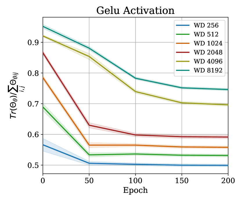
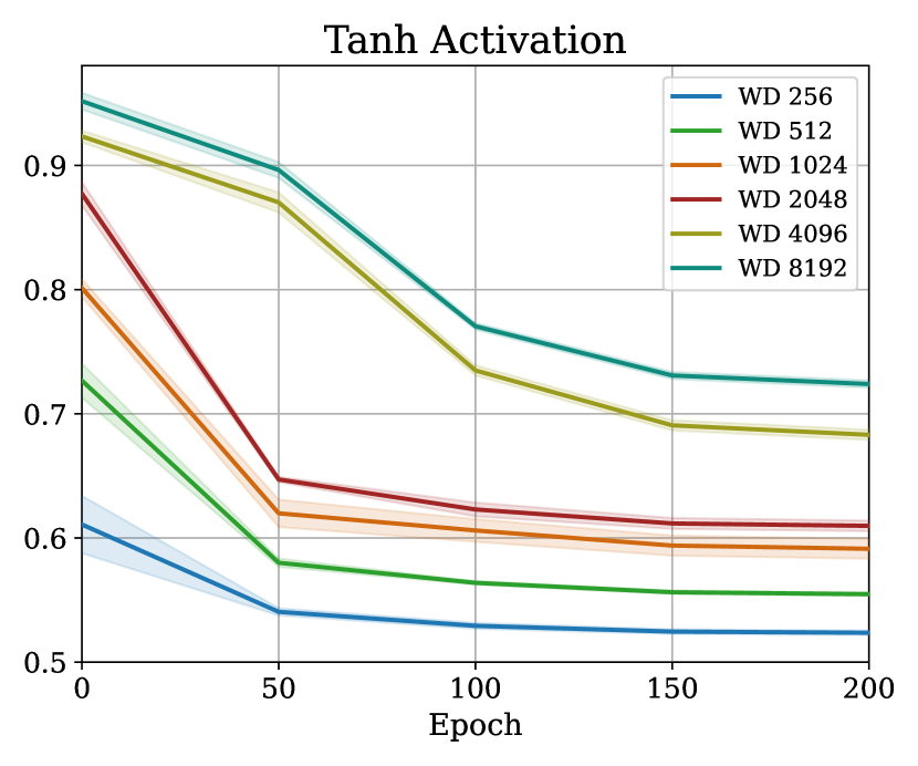
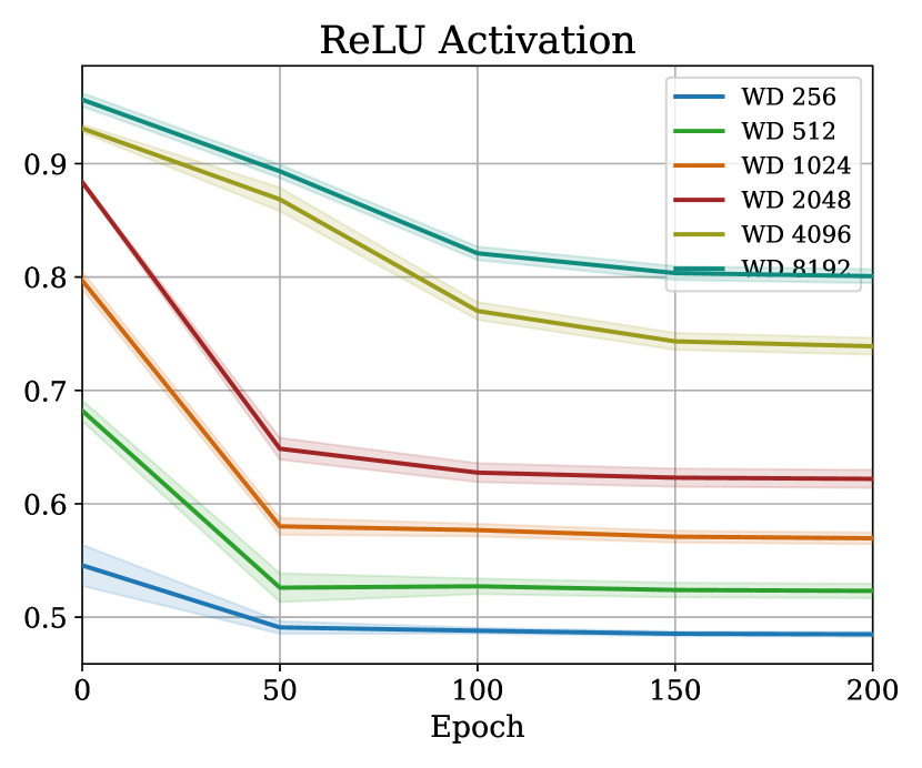
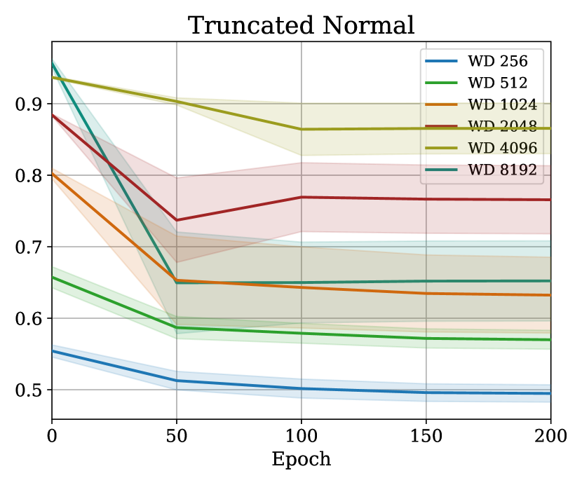
Figure 13: Comparing the magnitude of sum of on-diagonal and off-diagonal elements of $\Theta_{\theta}$ at initialization and throughout training, based on $1000$ points from CIFAR-10. The reported numbers are the average of $1000\times 1000$ kernels each having a shape of $10\times 10$. The same subset has then been used to train the NN using SGD.

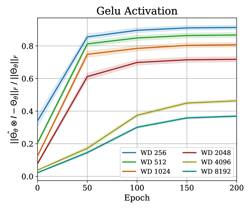
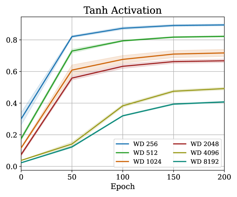
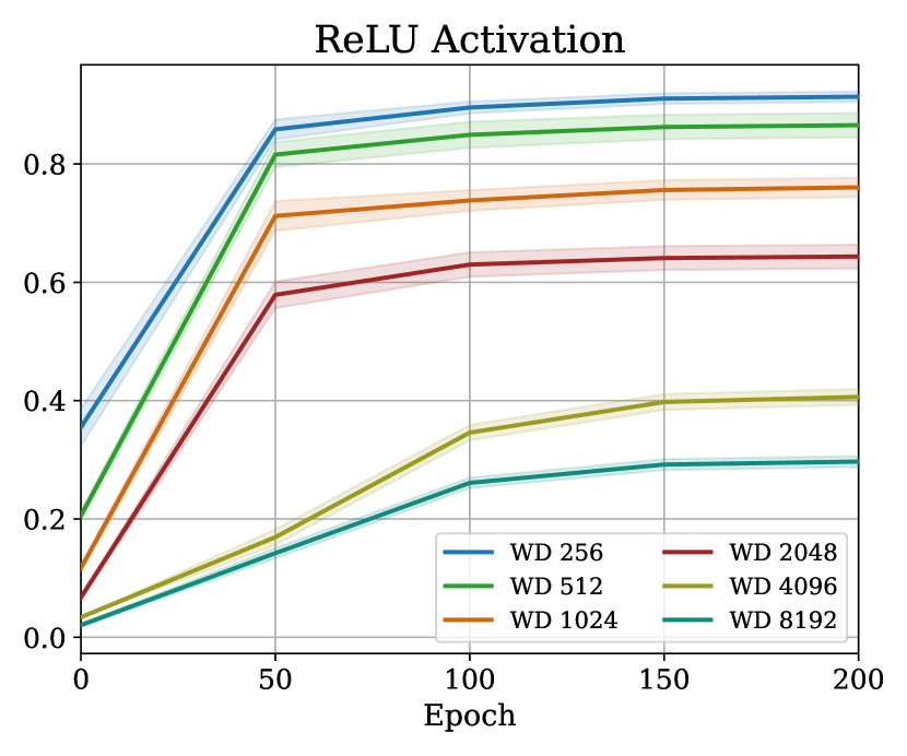
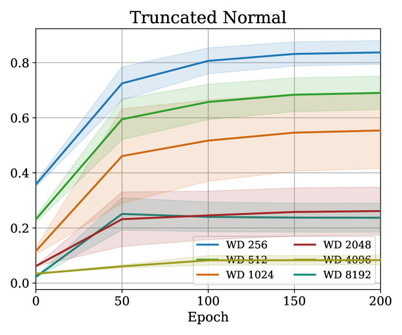
Figure 14: Evaluating the relative difference of Frobenius norm of $\Theta_{\theta}(\mathcal{D},\mathcal{D})$ and $\hat{\Theta}_{\theta}(\mathcal{D},\mathcal{D})\otimes I_{O}$ at initialization and throughout training, based on $1000$ points from CIFAR-10.

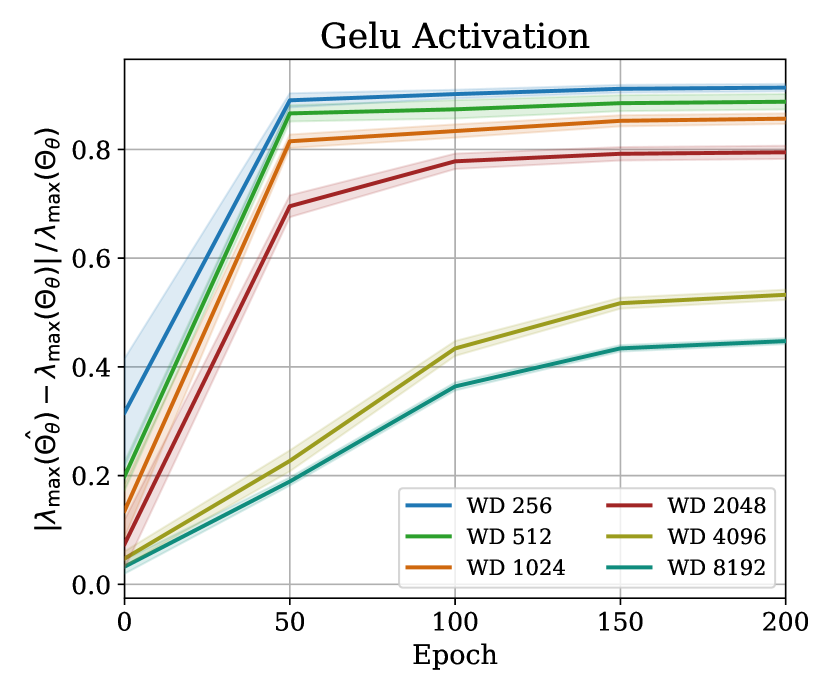
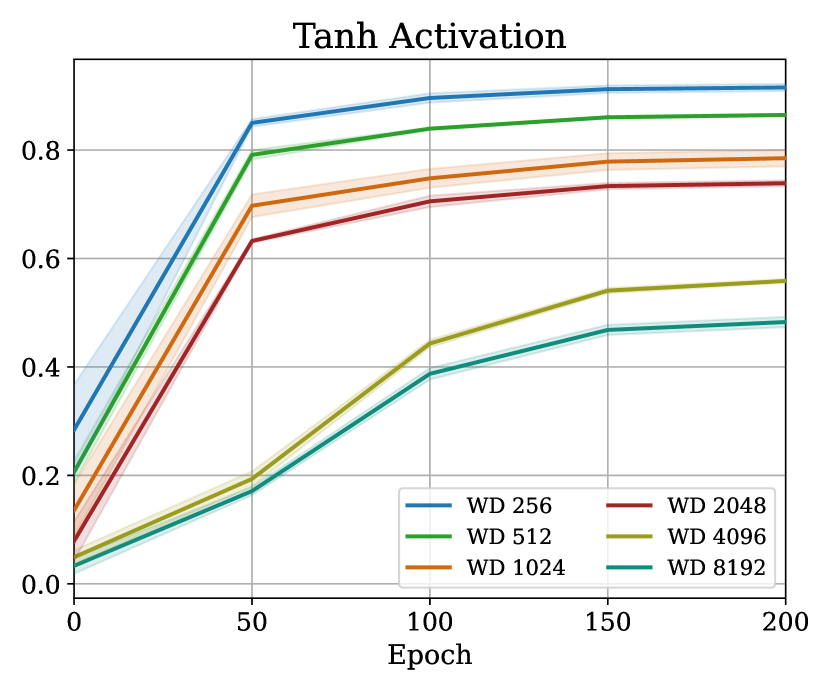
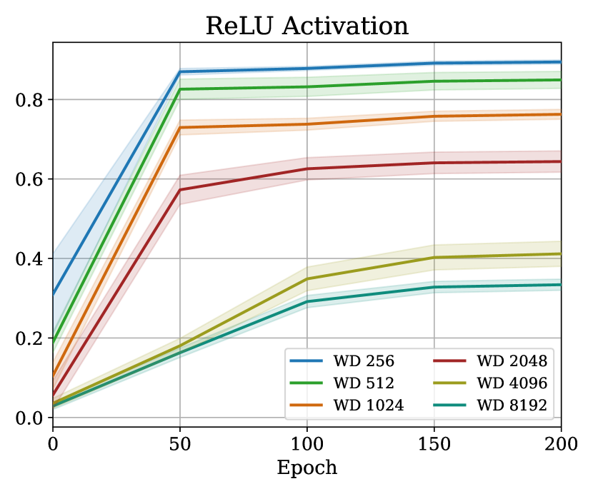
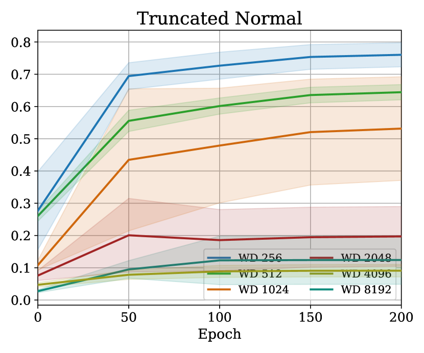
Figure 15: Evaluating the relative difference of $\lambda_{\max}$ of $\Theta_{\theta}(\mathcal{D},\mathcal{D})$ and $\hat{\Theta}_{\theta}(\mathcal{D},\mathcal{D})$ at initialization and throughout training, based on kernels on a subset ($\lvert\mathcal{D}\rvert=1000$) of points from CIFAR-10.

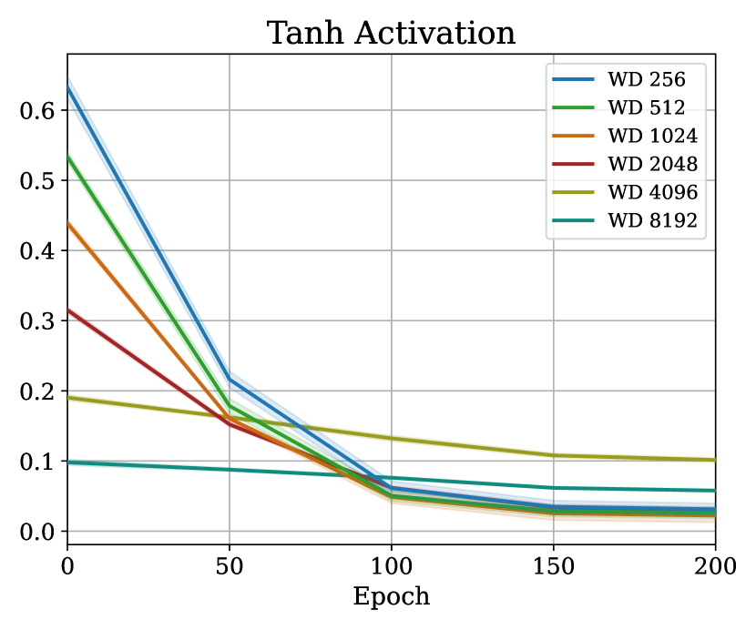
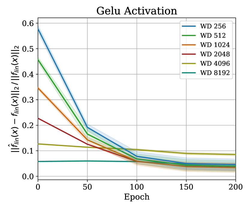
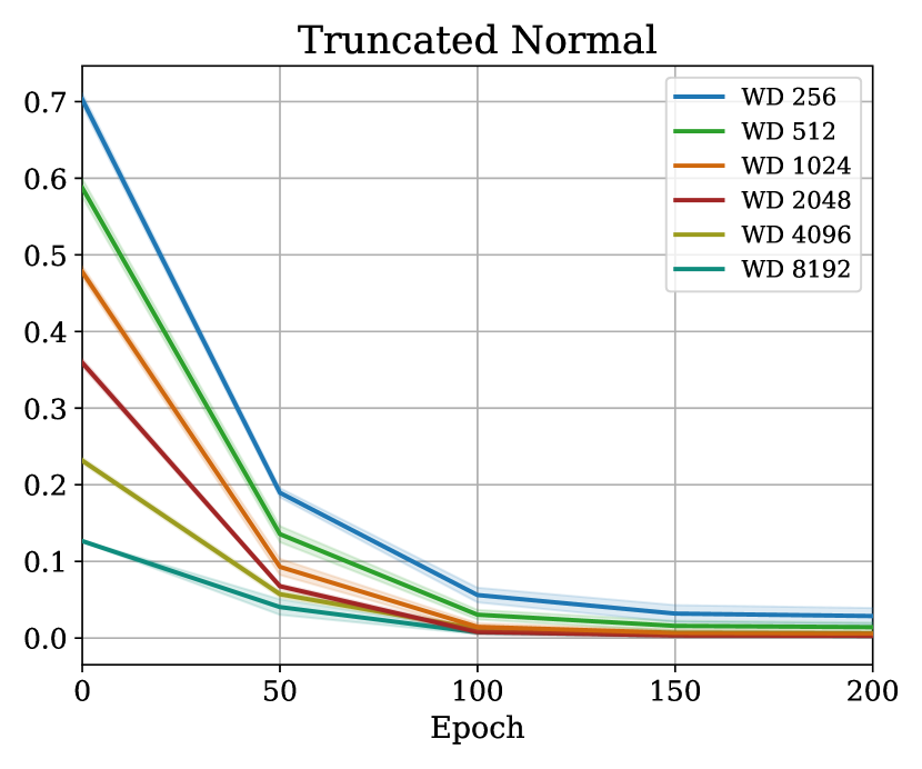
Figure 16: Evaluating the relative norm difference of kernel regression outputs using eNTK and pNTK as in Equation 4 and Equation 5 at initialization and throughout training. The kernel regression has been done on $\lvert\mathcal{D}\rvert=1000$ training points and $\lvert\mathcal{X}\rvert=500$ test points randomly selected from CIFAR-10’s train and test sets.

Appendix E Extending the Proofs to Other Architectures

We start our description of how to extend the proofs to other architectures by providing a sketch on how the dense weight vectors can be replaced by other layers of choice like convolutions. First, note how the linear weights are used in Equation 17. As mentioned in Section 6 of Yang (2020), we can accordingly write the same expansion for other forward computational graphs and derive the corresponding canonincal decomposition for them. In subsection 6.2.1, Yang (2020) provides a concrete example on how one can derive this expansion for a general RNN-like architecture. As the proofs provided in this section depend on the MLP structure only by means of the canonical decomposition, one can extend them to a general architecture by deriving the corresponding canonical decomposition of that architecture.

Non-Gaussian Weights: According to the strategy used in the proofs, we need the individual weights to be distributed such that the product of two independent scalar weights (as in Equation 17) remain sub-exponential. Hence, any sub-gaussian initialization method, such as any bounded initialization (e.g. truncated normal or uniform on an interval) can be used, and the same proof structure would support the same convergence rate, albeit with different constants in convergence (independent of $n$).

Non-ReLU activations: In general, the proofs rely on the ReLU activation through Lemma B.12, which gives a concentration bound on the absolute value of the dot product of post-activations of each layer of the NN. To use other nonlinearities, we would only need an analagous result for that nonlinearity; the other proofs follow without requiring any other significant change.

Experimental Evaluation: To provide further experimental support for this argument, we have conducted an ablation study on the FCN architecture with different nonlinearities and with truncated Gaussian initialization (Figures 13, LABEL:, 3, LABEL:, 15, LABEL: and 16). As seen in the provided figures, the impact of nonlinearity and initialization method as long as they follow the provided setting in A, is marginal.

Appendix F More Details on Kernel Regression Using pNTK on Full CIFAR-10 Dataset

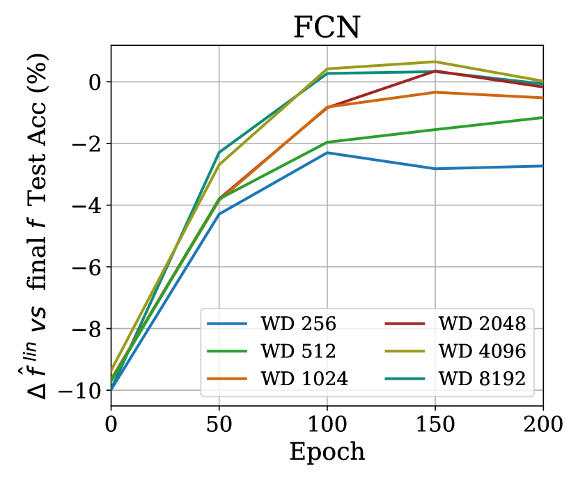
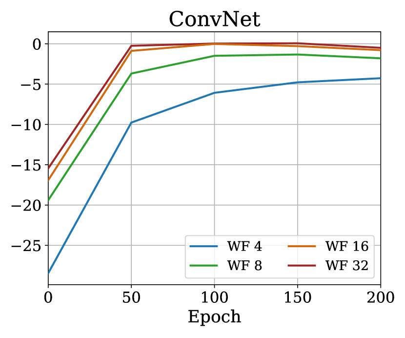
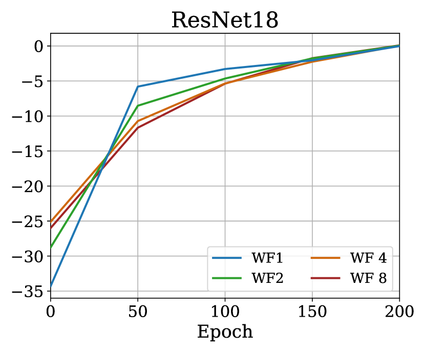
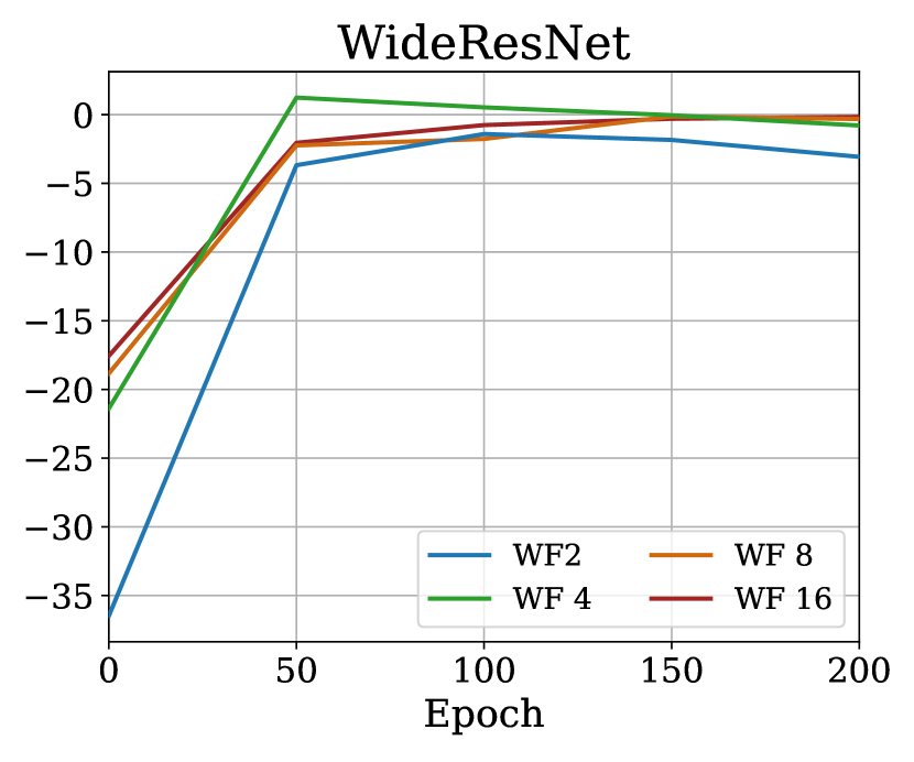
Figure 17: Evaluating the difference in test accuracy of kernel regression using pNTK as in (5) vs the final model $f$ throughout SGD training on the full CIFAR-10 dataset. How much worse would it be to “give up” on SGD at this point and train $\hat{f}^{\mathit{lin}}$ with the current representation?

Figure 17 compares the accuracy of $\hat{f}^{\mathit{lin}}(x)$ with parameters derived at epoch $E\in\{0,50,100,150,200\}$ of training the NN with SGD. On the y-axis, the reported number is $f^{\mathit{lin}}(x)-f^{*}(x)$ where $f^{*}$ denotes the final model obtained after training $f$ for 200 epochs. As seen in Figure 17 the architecture of the model has a significant impact on how good the linearization predicts the final accuracy of the fully-trained model. However, as proven in Theorem 4.1 in conjunction with the linearization approximations provided in Lee et al. (2019), as width grows, this approximation becomes more accurate. One unexplored fact regarding this experiment is that fact that lineraization with trained parameters significantly outperforms linearization at initialization, which is intuitive but not rigorously investigated yet.

Appendix G Experimental Evaluation: Tightness of bounds

Figure 18 presents experimental evaluations that analyze the tightness of the approximation bound. The results are presented for the fully connected network used in the experiment.

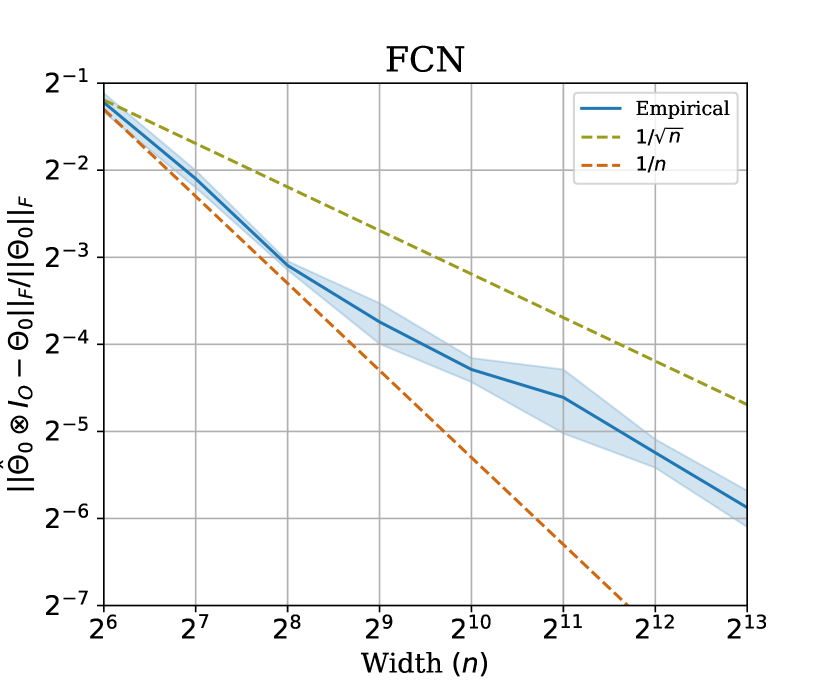
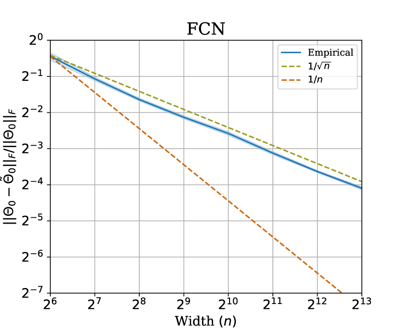
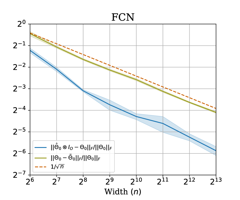
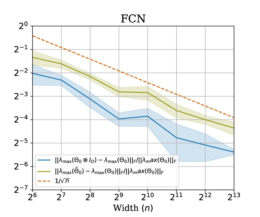
Figure 18: Experimental evaluation of tightness of approximation bounds

References

• Adlam et al. (2020) Adlam, B., Lee, J., Xiao, L., Pennington, J., and Snoek, J. Exploring the uncertainty properties of neural networks’ implicit priors in the infinite-width limit. arXiv:2010.07355, 2020.
• Álvarez et al. (2012) Álvarez, M. A., Rosasco, L., and Lawrence, N. D. Kernels for vector-valued functions: A review. Foundations and Trends® in Machine Learning, 4(3):195–266, 2012.
• Arora et al. (2019) Arora, S., Du, S. S., Hu, W., Li, Z., Salakhutdinov, R., and Wang, R. On exact computation with an infinitely wide neural net. In NeurIPS, 2019.
• Arora et al. (2020) Arora, S., Du, S. S., Li, Z., Salakhutdinov, R., Wang, R., and Yu, D. Harnessing the power of infinitely wide deep nets on small-data tasks. In ICLR, 2020.
• Arpit & Bengio (2019) Arpit, D. and Bengio, Y. The benefits of over-parameterization at initialization in deep ReLU networks. arXiv:1901.03611, 2019.
• Bachmann et al. (2022) Bachmann, G., Hofmann, T., and Lucchi, A. Generalization through the lens of leave-one-out error. In ICLR, 2022.
• Chen et al. (2021) Chen, X., Hsieh, C.-J., and Gong, B. When vision transformers outperform resnets without pre-training or strong data augmentations. In ICLR, 2021.
• Craven & Wahba (1978) Craven, P. and Wahba, G. Smoothing noisy data with spline functions. Numerische mathematik, 31(4):377–403, 1978.
• Deng et al. (2009) Deng, J., Dong, W., Socher, R., Li, L.-J., Li, K., and Fei-Fei, L. ImageNet: A large-scale hierarchical image database. In CVPR, 2009.
• Epperly (2022) Epperly, E. Note to self: Hanson–wright inequality, 2022. URL https://www.ethanepperly.com/index.php/2022/10/04/note-to-self-hanson-wright-inequality/.
• Fort et al. (2020) Fort, S., Dziugaite, G. K., Paul, M., Kharaghani, S., Roy, D. M., and Ganguli, S. Deep learning versus kernel learning: an empirical study of loss landscape geometry and the time evolution of the neural tangent kernel. In NeurIPS, 2020.
• Franceschi et al. (2022) Franceschi, J.-Y., de Bézenac, E., Ayed, I., Chen, M., Lamprier, S., and Gallinari, P. A neural tangent kernel perspective of GANs. In ICML, 2022.
• Hazan & Jaakkola (2015) Hazan, T. and Jaakkola, T. Steps toward deep kernel methods from infinite neural networks. arXiv:1508.05133, 2015.
• He et al. (2020) He, B., Lakshminarayanan, B., and Teh, Y. W. Bayesian deep ensembles via the neural tangent kernel. NeurIPS, 2020.
• He et al. (2015) He, K., Zhang, X., Ren, S., and Sun, J. Delving deep into rectifiers: Surpassing human-level performance on ImageNet classification. In ICCV, 2015.
• He et al. (2016) He, K., Zhang, X., Ren, S., and Sun, J. Deep residual learning for image recognition. In CVPR, 2016.
• Holzmüller et al. (2023) Holzmüller, D., Zaverkin, V., Kästner, J., and Steinwart, I. A framework and benchmark for deep batch active learning for regression. JMLR, 2023.
• Jacot et al. (2018) Jacot, A., Gabriel, F., and Hongler, C. Neural tangent kernel: Convergence and generalization in neural networks. In NeurIPS, 2018.
• Krizhevsky (2009) Krizhevsky, A. Learning multiple layers of features from tiny images. 2009.
• Lee et al. (2018) Lee, J., Bahri, Y., Novak, R., Schoenholz, S. S., Pennington, J., and Sohl-Dickstein, J. Deep neural networks as gaussian processes. In ICLR, 2018.
• Lee et al. (2019) Lee, J., Xiao, L., Schoenholz, S., Bahri, Y., Novak, R., Sohl-Dickstein, J., and Pennington, J. Wide neural networks of any depth evolve as linear models under gradient descent. In NeurIPS, 2019.
• Lee et al. (2020) Lee, J., Schoenholz, S., Pennington, J., Adlam, B., Xiao, L., Novak, R., and Sohl-Dickstein, J. Finite versus infinite neural networks: an empirical study. NeurIPS, 2020.
• Matthews et al. (2018) Matthews, A. G. d. G., Rowland, M., Hron, J., Turner, R. E., and Ghahramani, Z. Gaussian process behaviour in wide deep neural networks. In ICLR, 2018.
• Mohamadi et al. (2022) Mohamadi, M. A., Bae, W., and Sutherland, D. J. Making look-ahead active learning strategies feasible with neural tangent kernels. In NeurIPS, 2022.
• Neal (1996) Neal, R. M. Priors for infinite networks, pp.  29–53. Springer, 1996.
• Nguyen et al. (2021a) Nguyen, T., Chen, Z., and Lee, J. Dataset meta-learning from kernel ridge-regression. In ICLR, 2021a.
• Nguyen et al. (2021b) Nguyen, T., Novak, R., Xiao, L., and Lee, J. Dataset distillation with infinitely wide convolutional networks. NeurIPS, 2021b.
• Novak et al. (2019) Novak, R., Xiao, L., Lee, J., Bahri, Y., Yang, G., Hron, J., Abolafia, D. A., Pennington, J., and Sohl-Dickstein, J. Bayesian deep convolutional networks with many channels are Gaussian processes. In ICLR, 2019.
• Novak et al. (2022) Novak, R., Sohl-Dickstein, J., and Schoenholz, S. S. Fast finite width neural tangent kernel. In ICML, 2022.
• Park et al. (2019) Park, D., Sohl-Dickstein, J., Le, Q., and Smith, S. The effect of network width on stochastic gradient descent and generalization: an empirical study. In ICML, 2019.
• Park et al. (2020) Park, D. S., Lee, J., Peng, D., Cao, Y., and Sohl-Dickstein, J. Towards NNGP-guided neural architecture search. arXiv:2011.06006, 2020.
• Rudi et al. (2017) Rudi, A., Carratino, L., and Rosasco, L. FALKON: An optimal large scale kernel method. In NeurIPS, 2017.
• Tancik et al. (2020) Tancik, M., Srinivasan, P., Mildenhall, B., Fridovich-Keil, S., Raghavan, N., Singhal, U., Ramamoorthi, R., Barron, J., and Ng, R. Fourier features let networks learn high frequency functions in low dimensional domains. NeurIPS, 2020.
• Vershynin (2018) Vershynin, R. High-dimensional probability: An introduction with applications in data science. Cambridge University Press, 2018.
• Wainwright (2019) Wainwright, M. J. High-Dimensional Statistics: A Non-Asymptotic Viewpoint. Cambridge University Press, 2019.
• Wang et al. (2021) Wang, H., Huang, W., Margenot, A., Tong, H., and He, J. Deep active learning by leveraging training dynamics. 2021.
• Wei et al. (2022) Wei, A., Hu, W., and Steinhardt, J. More than a toy: Random matrix models predict how real-world neural representations generalize. In ICML, 2022.
• Williams (1996) Williams, C. Computing with infinite networks. NeurIPS, 9, 1996.
• Xiao et al. (2017) Xiao, H., Rasul, K., and Vollgraf, R. Fashion-MNIST: a novel image dataset for benchmarking machine learning algorithms. arXiv:1708.07747, 2017.
• Xiao et al. (2018) Xiao, L., Bahri, Y., Sohl-Dickstein, J., Schoenholz, S., and Pennington, J. Dynamical isometry and a mean field theory of CNNs: How to train 10,000-layer vanilla convolutional neural networks. In ICML, 2018.
• Xiao et al. (2020) Xiao, L., Pennington, J., and Schoenholz, S. Disentangling trainability and generalization in deep neural networks. In ICML, 2020.
• Yang (2019) Yang, G. Wide feedforward or recurrent neural networks of any architecture are Gaussian processes. NeurIPS, 2019.
• Yang (2020) Yang, G. Tensor Programs II: Neural tangent kernel for any architecture. arXiv:2006.14548, 2020.
• Yang & Littwin (2021) Yang, G. and Littwin, E. Tensor Programs IIb: Architectural universality of neural tangent kernel training dynamics. In ICML, 2021.
• Zagoruyko & Komodakis (2016) Zagoruyko, S. and Komodakis, N. Wide residual networks. BMVC, 2016.
• Zhou et al. (2021) Zhou, Y., Wang, Z., Xian, J., Chen, C., and Xu, J. Meta-learning with neural tangent kernels. In ICLR, 2021.