Causal Scoring: A Framework for Effect Estimation, Effect Ordering, and Effect Classification

Abstract

This paper introduces causal scoring as a novel approach to frame causal estimation in the context of decision making. Causal scoring entails the estimation of scores that support decision making by providing insights into causal effects. We present three valuable causal interpretations of these scores: effect estimation (EE), effect ordering (EO), and effect classification (EC). In the EE interpretation, the causal score represents the effect itself. The EO interpretation implies that the score can serve as a proxy for the magnitude of the effect, enabling the sorting of individuals based on their causal effects. The EC interpretation enables the classification of individuals into high- and low-effect categories using a predefined threshold. We demonstrate the value of these alternative causal interpretations (EO and EC) through two key results. First, we show that aligning the statistical modeling with the desired causal interpretation improves the accuracy of causal estimation. Second, we establish that more flexible causal interpretations are plausible in a wider range of settings and propose conditions to assess their validity. We showcase the practical utility of causal scoring through diverse scenarios, including situations involving unobserved confounding due to self-selection, lack of data on the primary outcome of interest, or lack of data on how individuals behave when intervened. These examples illustrate how causal scoring facilitates reasoning about flexible causal interpretations of statistical estimates in various contexts. They encompass confounded estimates, effect estimates on surrogate outcomes, and even predictions about non-causal quantities as potential causal scores.

1 Introduction

In recent years, we have seen an acceleration of research on machine learning (ML) methods for causal effect estimation at the individual level. A key motivation behind several of these methods is their use for decision making in application domains such as marketing (Lemmens and Gupta, 2020), medicine (Zhao et al., 2012), education (Olaya et al., 2020), and public policy (Bhattacharya and Dupas, 2012). With ML, decision makers can predict how responses to interventions vary from one individual to another and tailor interventions on a more granular level.

ML methods for causal estimation are often evaluated based on their ability to accurately predict causal effects (Dorie et al., 2019). However, a subtle (but critical) observation is that when effect predictions are used for decision making, their accuracy is not necessarily the primary concern. From a decision maker’s perspective, what matters is how potential errors in the predictions may affect the decision making, not how accurate the predictions themselves are.

The dichotomy between causal effect estimation and decision making is well illustrated by the following example, taken from Fernández-Loría and Provost, 2022b :

“Suppose a firm is willing to send an offer to customers for whom it increases the probability of purchasing by at least 1%. In this case, precisely estimating individual causal effects is desirable but not necessary; the only concern is identifying those individuals for whom the effect is greater than 1%. Importantly, overestimating (underestimating) the effect has no bearing on decision making when the focal individuals have an effect greater (smaller) than 1%.”

Fernández-Loría and Provost, 2022b go on to discuss the practical implications of this observation. The upshot is that thinking about the decision (rather than the causal effect) as the ultimate goal of the causal estimation is critical for choosing the appropriate ML method (Fernández-Loría et al., 2022), the appropriate training data (Fernández-Loría and Provost, 2019), and even the appropriate target variable (Fernández-Loría and Provost, 2022a ). The main insight of this series of papers is that “what might traditionally be considered good estimates of causal effects are not necessary to make good causal decisions” (Fernández-Loría and Provost, 2022b ).

What remains unclear is when we can use such “incorrect” causal estimates for the purposes of causal decision making; this large, important, and mostly understudied research question is the broad motivation of this paper. The essence of statistical causal inference lies in comprehending the data-generating processes (DGPs) that enable us to estimate causality from data. For most researchers and practitioners well-versed in causal inference, this amounts to answering the following question: Does the DGP meet the necessary conditions for interpreting the statistical estimates as causal effects? Well-known examples of such conditions are ignorability (Rosenbaum and Rubin, 1983), the back-door criterion (Pearl, 2009), or the necessary conditions for instrumental variables (IVs) to be valid (Angrist et al., 1996). The de facto perspective in the causal inference literature is that when the data is not suitable to estimate causal effects, then the statistical estimates should not be interpreted in a causal way.

We want to broaden this perspective. The main contribution of this paper is proposing a new statistical task called causal scoring as an innovative way of framing causal estimation (Section 2). We define causal scoring as the estimation of a quantity $\theta$ that relates to the causal effect $\beta$ in a way that is helpful to inform a decision-making process. We call $\theta$ a causal score and frame its causal interpretation in terms of its relationship with $\beta$:

• Effect estimation (EE): $\theta=\beta$. This standard causal interpretation of statistical estimates has prevailed in the causal inference literature. EE implies that the target of the statistical estimation ($\theta$) can be interpreted as a causal effect ($\beta$).

• Effect ordering (EO): Larger $\theta\Leftrightarrow$ Larger $\beta$. Under this causal interpretation, the causal score does not necessarily correspond to a causal effect but can be interpreted as a proxy for the magnitude of the causal effect. A larger causal score implies a larger causal effect, and vice versa. EO is a meaningful causal interpretation for decision-making processes where sorting individuals according to their causal effects is valuable. For example, the decision maker could be operating under resource constraints (e.g., limited budget, time, or attention) such that only the individuals on whom the intervention is predicted to have the largest effect should be considered.

• Effect classification (EC): $\theta>\tilde{\tau}\Leftrightarrow\beta>\tau$. The motivation behind many methods for causal effect estimation is to implement a decision-making policy to intervene on individuals for whom the intervention is predicted to have an effect greater than a threshold $\tau$. This is analogous to classifying individuals into the “high-effect” (positive) and “low-effect” (negative) classes. The EC causal interpretation implies that there exists a threshold $\tilde{\tau}$ that can be used on $\theta$ to make the same classifications as if $\beta$ and $\tau$ had been used.

A question that naturally arises from our proposal is, “How relevant are these alternative causal interpretations (EO and EC)?” This is an essential question because if the EE causal interpretation is valid, then the EO and EC causal interpretations are also valid. So, why should we care about any causal interpretation other than EE?

We provide two important reasons. The first is that the decision making can improve when the statistical modeling is guided by the specific causal interpretation we want from the causal scores. As explained by Fernández-Loría and Provost, 2022b , “by focusing on a specific task [decision making] rather than on a more general task [effect estimation], ML procedures can better exploit the statistical power available.” Fernández-Loría et al., (2022) explain and illustrate this observation by showing how methods designed for treatment assignment (EC) can generally lead to better causal decisions than methods designed for causal effect estimation (EE). In this paper, we expand these results and demonstrate that modeling causal scores for an EO interpretation can result in a better effect ordering than modeling for an EE interpretation (Section 5).

However, the most noteworthy argument in favor of alternative causal interpretations is that an EE interpretation is valid in more restrictive situations. A Venn diagram in Figure 1 illustrates the universe of situations where each causal interpretation is valid, showing that the EC and EO interpretations are valid under more cases than the EE interpretation. This observation is critical because obtaining appropriate data to estimate causal effects can be hard. Data can be unsuitable for causal effect estimation for a myriad of reasons: confounding, selection bias, treatment assignments affecting multiple units simultaneously, poor external validity, limitations in the experimental design, and so on. For example, although targeted advertising often involves experimentation, conducting controlled experiments to collect the necessary data to estimate causal effects can be prohibitively expensive (Gordon et al., 2022). Therefore, advertisers frequently rely on targeting ads based on conversion rates rather than ad effects, even when they can precisely estimate the causal effect of their ad campaigns  (Stitelman et al., 2011). Other limitations, such as optimizing for long-term outcomes, can also hinder decision makers from collecting data on the outcome of interest, even when controlled experiments are feasible (Yang et al., 2020).

Figure 1: Venn diagram illustrating the sets of situations where different causal interpretations are valid. EC and EO are valid in a wider range of situations than EE.

Fortunately, causal interpretations such as EO and EC could still be valid in these settings, and depending on the nature of the decision-making problem, these alternative interpretations could be all the decision maker really needs from the causal scores. We demonstrate the value of our causal scoring framework by formalizing conditions where an EO interpretation could be valid when an EE interpretation is clearly not (Section 3). These conditions are more general and weaker than any set of conditions that would allow us to interpret causal scores as causal effects, so they should hold in more situations than the ones typically considered in observational studies.

We then use these conditions to demonstrate how to assess the possibility of ordering individuals based on the magnitude of their intervention effects in various scenarios, including cases where:

1. There is no data on how people behave when intervened, but predictions of behavior without intervention could serve as causal scores (Section 4.1).

2. There is no data on the primary outcome of interest, but predictions of the intervention effect on a surrogate (proxy) outcome could serve as causal scores (Section 4.2).

3. There is unobserved confounding due to self-selection, but either the propensity to self-select or confounded estimates of the intervention effect could serve as causal scores (Section 4.3).

We also provide an empirical illustration in the context of advertising where decision making based on such “problematic” causal scores yields results comparable or even superior to those obtained from causal scores that conform to the EE interpretation (Section 6). Finally, in Section 7, we discuss the implications of our framework for data-driven decision making and future research.

This study highlights that causal inference involves more than simply estimating causal effects. While causal effect estimation is important, it is often a means to facilitate decision making, not an end in itself. Alternative causal interpretations of statistical estimates can be informative for decision making, even if the estimates themselves should not be interpreted as causal effects. However, as a research community addressing statistical causal inference, our knowledge of how to derive causal interpretations beyond effect estimation is rather limited. This study is an initial step toward addressing this gap, as it proposes causal scoring as a framework for more comprehensive causal interpretations of statistical estimates. We hope others will build on the framework and join us in advancing this important area of research.

2 Causal Scoring

We frame decision making from the perspective of a utilitarian social planner who seeks to maximize the mean welfare of a treatment allocation, as described by Manski, (2004). In this general problem formulation, the treatment could represent a medical intervention, an advertisement, or the allocation of a limited resource. The planner, who we will henceforth refer to as the decision maker, observes a vector $X$ of $m$ attributes (features) for each individual, where $X\in\mathbb{R}^{m}$. We consider cases where mean welfare is maximized by the treatment allocation:

$$a^{*}(x)\in\{0,1\},$$ (1)

where $a^{*}(x)=1$ if treating an individual with $X=x$ leads to an increase in mean welfare, and $a^{*}(x)=0$ otherwise.

We define the conditional average treatment effect (CATE) in terms of the potential outcomes $Y^{0}\in\mathbb{R}$ and $Y^{1}\in\mathbb{R}$ when untreated and treated, respectively (Rubin, 1974):

$$\begin{split}\beta(x)&=\mathbb{E}[Y^{1}-Y^{0}\mid X=x]\\ &=\mathbb{E}[C\mid X=x],\end{split}$$ (2)

where $C$ is the individual-level causal effect. We assume that treating an individual with $X=x$ leads to an increase in mean welfare when the CATE is greater than some quantity $\tau$, so:

$$a^{*}(x)=\mathbf{1}\{\beta(x)>\tau\},\forall x\in\mathbb{R}^{p}.$$ (3)

We assume that the decision maker can estimate the expectation of a scoring variable $S\in\mathbb{R}$ consistently and without bias. Critically, $S$ may or may not correspond to $C$. The conditional average score (CAS) or causal score refers to the expectation of $S$:

$$\theta(x)=\mathbb{E}[S\mid X=x].$$ (4)

Note that $\theta(x)$ is an estimand, not an estimate. Causal scoring is the estimation of a causal score $\theta$ that is informative of the causal effect $\beta$ in a way that is useful to implement the policy $a^{*}$. We refer to the information provided by $\theta$ regarding $\beta$ as the causal interpretation of the causal score.

We will first discuss the most straightforward causal interpretation one could give to causal scores. Specifically, the CAS has a valid effect estimation (EE) interpretation when:

$$\begin{split}\theta(x)=\beta(x),\forall x\in\mathbb{R}^{p},\end{split}$$ (5)

meaning that the causal scores and the causal effects are the same.

Our ability to causally interpret the CAS depends critically on its statistical formulation and the underlying assumptions about the DGP. For example, suppose the decision maker is considering estimating the CATE as the difference between groups of treated and untreated individuals. The CAS in this case corresponds to:

$$\begin{split}\theta(x)&=\mathbb{E}[Y\mid T=1,X=x]-\mathbb{E}[Y\mid T=0,X=x]\\ &=\mathbb{E}\left[\frac{YT}{\mathbb{P}[T=1\mid X=x]}-\frac{Y(1-T)}{\mathbb{P}[T=0\mid X=x]}\;\middle|\;X=x\right]\end{split}$$ (6)

where $T$ is the treatment assignment ($T=1$ for treated individuals, and $T=0$ for untreated individuals), and $Y=Y^{1}T+Y^{0}(1-T)$ is the observed outcome on historical data.

The CAS formulated in Equation (6) has a valid EE interpretation when the potential outcomes are conditionally independent of the treatment assignment given the features:

$$T\perp\!\!\!\perp Y^{0},Y^{1}\mid X.$$ (7)

This (non-testable) assumption about the DGP is known as unconfoundedness, ignorability (Rosenbaum and Rubin, 1983), the back-door criterion (Pearl, 2009), and exogeneity (Wooldridge, 2015). This assumption is met when the treatment assignment does not provide any information about the potential outcomes after conditioning on the features. If this is not the case, then the CAS as formulated in Equation (6) does not have a valid EE interpretation. Possible solutions include exploring other formulations for the CAS (e.g., an IV formulation) or collecting additional data where Equation (7) would be more plausible (e.g., by conducting a controlled experiment).

However, suppose the decision maker simply cannot obtain any data where an EE interpretation is valid, for any of the reasons we discussed in Section 1. What should the decision maker do then? Should they completely abandon any attempt at causal estimation and proceed to make decisions without data? Or should they use the CAS as the CATE in their decision making even though an EE interpretation is clearly invalid?

The literature on causal inference offers surprisingly little guidance regarding the use of confounded estimates for decision making. While some studies have discussed the potential value of confounded estimates for decision making (Fernández-Loría and Provost, 2019, Yang et al., 2020), they have not detailed under what DGPs the use of confounded estimates could be appropriate, nor have they offered tools to aid in the causal interpretation of confounded estimates. Typically, when causal estimates are known to be confounded, researchers tend to discard them altogether and avoid attributing any causal interpretation to them.

This paper aims to challenge this conventional view. As noted, effect estimates need not be entirely accurate to effectively support decision making. Therefore, our approach is to relax the requirements of the causal interpretation of the CAS in a way that its interpretation is still meaningful for decision making. For example, maybe the CAS cannot be interpreted as the CATE but can still be interpreted as proportional to the magnitude of the CATE. The main advantages of “weaker” causal interpretations is that they can be satisfied in a wider range of DGPs and allow us to consider a wider range of scoring variables beyond causal effect estimates. For instance, we may even consider “non-causal” predictions as the scoring variable (Athey et al., 2023), as we discuss in Section 4.1. With this goal in mind, we next introduce two new causal interpretations.

Based on the optimal policy defined in Equation (3), the CAS is relevant if it can help classify individuals into high-effect ($\beta(x)>\tau$) and low-effect ($\beta(x)\leq\tau$) groups. The CAS has a valid effect classification (EC) interpretation when:

$$\exists\tilde{\tau}:\theta(x)>\tilde{\tau}\Leftrightarrow\beta(x)>\tau,\forall x\in\mathbb{R}^{p},$$ (8)

meaning that there exists a threshold $\tilde{\tau}$ that can be combined with the CAS to classify individuals into high-effect and low-effect groups, as defined by $\tau$. As an example, suppose we define $\tau$ as the $k$-th largest CATE and $\tilde{\tau}$ as the $k$-th largest CAS. The EC interpretation is valid if the $k$ individuals with the largest CAS are also the $k$ individuals with the largest CATE.

Figure 2 illustrates this example. The blue solid line is the CAS as a function of the CATE. The vertical dashed line is the $k$-th largest CATE, and the horizontal dashed line is the $k$-th largest CAS. The $k$ individuals with the largest scores also correspond to the individuals with the largest effects if the blue line appears only on the upper-right quadrant and the lower-left quadrant. In this example, the CAS can be used to correctly identify the $k$ individuals with the largest CATEs, even though the causal scores should not be interpreted as effects.

Figure 2: Comparison of the CATE and the CAS. The CAS does not approximate the CATE accurately but can be used to identify the individuals with the largest CATEs (upper-right quadrant).

One complication with the EC interpretation is that its validity may depend on $\tau$. For instance, if $\tau=3$ or $\tau=5$ in Figure 2, then there is no $\tilde{\tau}$ that can be combined with the CAS to perfectly classify individuals into high- or low-effect groups. The next causal interpretation we introduce overcomes this issue. The CAS has a valid effect ordering (EO) interpretation when:

$$\theta(x_{i})>\theta(x_{j})\Leftrightarrow\beta(x_{i})>\beta(x_{j}),\forall x_{i},x_{j}\in\mathbb{R}^{p},$$ (9)

meaning that ordering individuals according to their CAS is the same as ordering them according to their CATE. In other words, a larger CAS always corresponds to a larger CATE.

Theorem 1.

If the CAS has a valid EO interpretation, then it also has a valid EC interpretation for any $\tau$.

The proof is in Appendix A. This theorem implies that an EC interpretation can be achieved regardless of $\tau$ when the CAS has a valid EO interpretation, as illustrated by Figure 3. In contrast to Figure 2, Figure 3 shows that the $k$ individuals with the largest CAS always correspond to the $k$ individuals with the largest CATE. That is, for any $\tau$, there exists a $\tilde{\tau}$ for which the CAS has a valid EC interpretation.

When the decision maker’s primary concern is to give causal scores an EC interpretation, a practical question that arises is how to determine $\tilde{\tau}$. If the decision maker only intends to target the top $k$ individuals with the largest effects (e.g., due to resource constraints), then $\tau$ is the $k$-th largest CATE, and a CAS with a valid EO interpretation will also have a valid EC interpretation if we set $\tilde{\tau}$ as the $k$-th largest CAS. However, in cases where $\tau$ corresponds to a fixed quantity, what value to set for $\tilde{\tau}$ may not be immediately clear. We discuss such cases in Section 7.

Figure 3: The CAS preserves the ranking of the CATEs. So, there always exists a $\tilde{\tau}$ to optimally classify individuals into “treat” (upper-right corner) and “not treat” (lower-left corner) decisions.

3 Sufficient Conditions for Effect Ordering

We next derive general conditions under which an EO interpretation is valid. These conditions provide a framework for a decision maker to theoretically assess if an EO causal interpretation of the CAS is justified in a specific context, akin to how non-testable assumptions are used in observational studies to assess if statistical estimates can be interpreted as causal effects. However, the conditions we propose are more general because the requirements of the causal interpretation are less strict; if the conditons are met, then the CAS can be used for effect ordering but not necessarily for effect estimation.

3.1 Full Latent Mediation and Latent Synchrony

One way to conceptualize the CAS is as a statistical surrogate for the relationship between the set of features $X$ and the CATE. Surrogates, also known as surrogate markers, are commonly employed in clinical trials when the primary outcome of interest is highly undesirable (such as death) or when the occurrence of such events is extremely low, making it impractical to conduct a clinical trial with a statistically significant number of measured outcomes (Prentice, 1989). The rationale behind using a surrogate is that the impact of the intervention on the surrogate can predict its effect on the clinical outcome of interest.

However, our specific objective differs slightly, as we aim to simply describe the statistical dependence between the features $X$ and the CATE. We are not asserting that intervening on $X$ will necessarily amplify the magnitude of the CATE, but rather that certain values of $X$ are associated with greater causal effects. In this context, we can view the CAS as a statistical surrogate for this relationship: variations in $X$ associated with changes in the CAS provide valuable insights into corresponding changes in the CATE.

Traditional causal frameworks focus primarily on characterizing DGPs in which the CAS and the CATE are exactly the same: $\theta(X)=\beta(X)$. We refer to this scenario as an instance of full causal mediation, as it assumes that the relationship between $X$ and the CATE is fully mediated by the CAS, as depicted in Figure 4(a). However, when confounding factors are present, it becomes concerning that variations in the scores may not correspond to similar changes in effects, thereby rendering the scores unsuitable for interpretation as effects. Figure 4(b) illustrates an example of such a situation. In what follows, we propose conditions under which the CAS maintains a valid EO interpretation even in the absence of full causal mediation.

(a) Full causal mediation.

(b) No mediation.

Figure 4: Full causal mediation vs. no mediation. Existing causal frameworks are exclusively focused on describing conditions where full causal mediation is met, which means the relationship between the features $X$ and the causal effect of interest $\beta(X)$ is fully explained by the causal scores $\theta(X)$.

These conditions require us to define a latent mediator $L$ through which $C$, $S$, and $X$ relate:

$$L=\mu(X)+\epsilon,$$ (10)

where $\mu(X)$ is the expectation of $L$ given $X$, and $\epsilon$ is random variation in $L$ that cannot be explained by $X$ and, therefore, is independent of $X$. Our first condition is that $C$ and $S$ are mean independent of $X$ given the latent mediator $L$:

$$\begin{split}\mathbb{E}[C\mid L,X]&=\mathbb{E}[C\mid L],\\ \mathbb{E}[S\mid L,X]&=\mathbb{E}[S\mid L].\end{split}$$ (11)

We refer to this condition as full latent mediation. It is important to note that the decision maker is not required to directly observe the variable $L$. The crucial factor is the existence of a variable $L$ that satisfies Equation (11). This condition aligns with the primary criterion established by Prentice, (1989) for defining a valid surrogate, which states that the outcome of interest is conditionally independent of the treatment assignment given the surrogate. In our case, full latent mediation is achieved when there is a shared, valid surrogate for both the CAS and the CATE, which may potentially remain unobserved.

Lemma 1.

Full latent mediation implies that there exist functions $g$ and $h$ such that:

$$\begin{split}\beta(X)&=g(\mu(X)),\\ \theta(X)&=h(\mu(X)).\end{split}$$ (12)

The proof is in Appendix B. Figure 5 shows the DGP implied by Lemma 1. Under this DGP, the only reason why $X$ gives information about the causal effects or the causal scores is because of $L$. The implication is that there is a latent predictor that fully explains why the CATE and the CAS vary as $X$ varies. Although at first this may seem like a strong assumption, it is actually a generalization of the full causal mediation assumption (Figure 4(a)) that is prevalent in all existing causal frameworks. Full causal mediation corresponds to full latent mediation with $L=C$.

Figure 5: Full latent mediation. The features in $X$ only provide information about the causal effects $\beta(X)$ and the causal scores $\theta(X)$ through a latent predictor $\mu(X)$. This is a generalization of full causal mediation.

The next condition we introduce is latent synchrony. Let $g_{\Delta}=g(\mu(x_{i}))-g(\mu(x_{j}))$ and $h_{\Delta}=h(\mu(x_{i}))-h(\mu(x_{j}))$ represent the change in $g$ and $h$ for given points $x_{i}$ and $x_{j}$. Latent synchrony is defined as:

$$\begin{split}\frac{h_{\Delta}}{g_{\Delta}}>0,\quad\forall x_{i},x_{j}.\\ \end{split}$$ (13)

This condition implies that the causal effects and the causal scores have the same qualitative relationship with the latent mediator. Specifically, as the expectation of $L$ given $X$ changes, both $\beta$ and $\theta$ either increase together or decrease together. For example, if $g$ and $h$ are both strictly increasing or decreasing functions, then Equation (13) is met.

Theorem 2.

If full latent mediation and latent synchrony are met, then the CAS has a valid EO interpretation.

The proof is in Appendix C. Theorem 2 formalizes conditions for an EO interpretation. These proposed conditions are sufficient (not necessary), so an EO interpretation could be valid even in DGPs where these conditions do not hold. In contrast, full causal mediation is a strictly stronger condition that is necessary for an EE interpretation to be valid. This has important implications for the generality of our proposed conditions, as formalized below (proof in Appendix D).

Proposition 1.

Full latent mediation and latent synchrony hold in all DGPs where an EE interpretation is valid, with $L=\theta(X)$.

This result implies that full latent mediation and latent synchrony are weaker and more general conditions than any of the conditions typically used in observational studies to assess if statistical estimates can be interpreted as causal effects.

4 Assessment of Alternative Causal Interpretations

In this section, we discuss multiple examples showcasing the utility of full latent mediation and latent synchrony to assess appropriate causal interpretations when unbiased effect estimation is impossible due to data limitations. Our discussion encompasses diverse scenarios and types of causal scores, including cases where:

1. There is no data on individuals’ behavior under treatment, but predictions of behavior without intervention could serve as causal scores (Section 4.1).

2. There is no data on the target outcome, but predictions of the treatment effect on a surrogate (proxy) outcome could serve as causal scores (Section 4.2).

3. There is unobserved confounding due to self-selection, and possible causal scores are the propensity to self-select or confounded estimates of the treatment effect (Section 4.3).

Furthermore, we examine cases where violations of full latent mediation and latent synchrony undermine the validity of an EO interpretation. In each example, we delve into the factors that may exacerbate or mitigate the severity of the violations. Additionally, we explore the prospect of embracing more cautious causal interpretations in these circumstances.

4.1 Example 1: Predicting baseline outcomes for nudging

In our first example, we consider the use of causal scoring for nudging. Guiding user behavior through personalized nudges is one of the most widespread and prominent uses of machine learning. Found in advertising, product recommendations, adaptive learning, fitness apps, and more, nudging plays a crucial role in shaping user choices across various aspects of life.

Consider the scenario where the nudge is designed to influence an agent’s binary decision (e.g., to exercise or not, to make a purchase or not). Drawing on discrete choice modeling Train, (2009), one approach to model the influence of the nudge is as follows:

$$Y=\mathbf{1}\{U+\delta T>0\}.$$ (14)

In Equation (14), $Y$ represents the agent’s decision, where $Y=1$ signifies the specific choice the nudge aims to encourage. The variable $T$ represents whether the agent is nudged, taking the value $1$ if nudged and $0$ otherwise. The agent’s utility gain from choosing $Y=1$ over $Y=0$ is denoted by $U+\delta T$, and the agent opts for $Y=1$ if the utility gain is greater than 0. The parameter $\delta$ serves to quantify the causal impact of the nudge on the agent’s utility gain in the event of choosing $Y=1$. It’s worth noting that while $\delta$ remains constant across all agents, the effect of $T$ on $Y$ varies among individuals due to its dependence on the unobservable variable $U$. We will address the scenario where $\delta$ is not constant later in this section.

Suppose the decision maker (the “nudger”) wants to identify the individuals on whom the nudge effect on $Y$ is the largest. This would facilitate targeted interventions while operating under constraints like a restricted budget of time or attention. Additionally, it could also help in the development of alternative messages tailored to cases where the nudge is less effective.

The decision maker does not observe $U$ but has access to a set of agent attributes $X$ (features) that are correlated with $U$. There is also historical data on past agent decisions, but the use of nudges has not been implemented previously, so estimating the effect of the nudge is unfeasible. However, what the decision maker can do is estimate the following CAS:

$$\begin{split}\theta(x)&=\mathbb{P}[Y=1\mid T=0,X=x]\\ &=\mathbb{P}[Y^{0}=1\mid X=x],\end{split}$$ (15)

which corresponds to the probability of the agent making the desired choice without a nudge.

Although an EE interpretation is clearly invalid in this case, the CAS in Equation (15) is often used to infer the effect ordering of individuals across various contexts, including precision medicine, sales team prioritization, and the allocation of advertising budgets. The main appeal of this predictive (non-causal) approach is its applicability in cases where the treatment has never been tried before, or for which limited or non-representative historical data is available. For example, experimentation is common in advertising, but collecting sufficient data to precisely predict ad effects for each individual is a challenging endeavor that advertisers often consider prohibitively expensive or even impossible due to technical challenges (Gordon et al., 2022). As a result, targeted advertising is often based on predicted conversion rates rather than ad effects on conversion rates, which would correspond to the CAS in Equation (15).

Let’s now use full latent mediation and latent synchrony to assess whether an EO interpretation is reasonable in our context. In Equation (14), $U$ acts as a full latent mediator: $X$ only gives information about $Y^{0}$ (the scoring variable) and $C$ through $U$. However, assessing latent synchrony is a more intricate process, requiring us to examine the causal effect of the nudge in more detail.

Consider the function $\mu(X)=\mathbb{E}[U\mid X]$, representing the expected utility gain when an agent chooses $Y=1$. In Figure 6, we depict the CATE and the CAS as functions of $\mu(X)$ for a logit model with $\delta=0.5$. Higher values of $\mu(X)$ consistently lead to a greater CAS, while the CATE exhibits a bell-shaped curve. It’s crucial to recall that the nudge influences the agent’s decision only when it propels the utility gain beyond the “finish line,” prompting a shift from $Y=0$ to $Y=1$. This shift is more likely to occur for agents with an expected utility gain close to $-\delta/2$, which corresponds to the center of the bell-shaped curve.

In contrast, the nudge is ineffective for individuals with extremely low (high) utility gains who steadfastly adhere to their choices. On the left side of the curve, individuals are likely to choose $Y=0$ despite the nudge (“Lost Causes”), while those on the right are likely to choose $Y=1$ regardless of the nudge (“Sure Things”). This aligns with empirical evidence from Athey et al., (2023), documenting similar behavior when nudging students to seek financial aid renewal.

Figure 6: A larger expected utility gain implies a higher probability of the desired choice without a nudge (larger CAS), but not necessarily a larger causal effect on the agent’s decision (larger CATE). Latent synchrony does not universally hold but can occur when expected utility is generally low or high for everyone.

The primary implication is that latent synchrony does not hold in general. However, latent synchrony can still hold if $\mu(X)<-\delta/2$ for all individuals in the population. In this case, a larger $\mu(X)$ will consistently imply a larger CATE. This observation sheds light on the effectiveness of non-causal models for targeted advertising. In marketing applications, even the individuals with the highest probability of conversion typically exhibit single-digit conversion rates, conveying that $\mu(X)$ is low across the entire population. Consequently, those with the highest probability of converting without the ad are also the most likely to be influenced by the ad. Advocates of causal-effect models for marketing applications also recognize the effectiveness of non-causal models for effect ordering:

“A situation we commonly see in retail environments is that direct marketing activity appears to have the most positive effect on high-spending customers. Where this is the case, [causal effects] and sales are positively correlated, and therefore a conventional model and [a causal] model are more likely to rank the population in similar ways.” (Radcliffe and Surry, 2011)

Therefore, an EO interpretation of a non-causal CAS (Equation (15)) can be reasonable for nudging applications where most individuals fall on the left side of Figure 6, as latent synchrony is more likely to be met in such scenarios. Similarly, for nudging applications where most individuals fall on the right side of Figure 6, an EO interpretation of a non-causal CAS could also be reasonable by reversing the ranking (i.e., individuals with the smallest CAS have the largest effects).

Nevertheless, let’s consider the case where latent synchrony is violated. Even in this case, the consequences may not be dire for the decision maker. Figure 7 illustrates the relationship between the CAS and the CATE in a scenario where the CAS varies from 0% to 60%. While the figure demonstrates that a larger CAS doesn’t necessarily correspond to a larger CATE, it shows that a CAS exceeding 28% consistently leads to a CATE larger than 11%. Consequently, an EC interpretation may still be valid, as the CAS could potentially serve in categorizing individuals into high-effect and low-effect groups.

Figure 7: A larger CAS does not always imply a larger CATE, so an EO interpretation is invalid. However, a CAS greater than 28% always implies a CATE greater than 11%, so an EC interpretation may still be valid.

In a broader sense, the validity of the EC interpretation relies on $\tau$ and $\tilde{\tau}$, which represent the thresholds for the CATE and the CAS, respectively. In this specific case, an EC interpretation holds only for cases where $\tau<11\%$. Otherwise, there is no $\tilde{\tau}$ for which the EC interpretation remains applicable. The determination of $\tau$ may involve considerations of benefit-cost trade-offs or the limitations imposed by the decision maker’s constrained resources. For instance, if the decision maker is restricted to targeting only $k$ individuals due to limited resources, $\tau$ corresponds to the $k$-th largest CATE, and $\tilde{\tau}$ corresponds to the $k$-th largest CAS. In this scenario, an EC interpretation is more likely to hold for larger budgets, corresponding to a higher value of $k$, as those values of $k$ also translate to smaller values of $\tau$ and $\tilde{\tau}$.

Finally, let’s explore a situation where the assumption of full latent mediation is violated. In Equation (14), we initially considered a fixed causal impact of the nudge on the agent’s utility gain, denoted by $\delta$. Now, let’s examine a scenario where this impact varies among agents:

$$Y=\mathbf{1}\{U+U_{\delta}T>0\}.$$ (16)

Here, in Equation (16), the constant $\delta$ has been replaced with the random variable $U_{\delta}$. Critically, if $X$ is informative of $U_{\delta}$, $U$ will no longer be a full latent mediator between $X$ and $C$.

How much will this influence the effect ordering? Consider that the heterogeneity in $C$ (the effect on the agent’s decision) is now influenced by two factors: variations in how agents feel about $Y=1$ to begin with (represented by $U$), and variations in the nudge’s effectiveness in making $Y=1$ more appealing to the agent (represented by $U_{\delta}$). These variations are partially captured by $X$ in terms of $\mu(X)=\mathbb{E}[U\mid X]$ and $\delta(X)=\mathbb{E}[U_{\delta}\mid X]$. If variations in $\mu(X)$ are more prominent than variations in $\delta(X)$, the rank correlation between the CAS and the CATE may remain robust despite the violation of full latent mediation. Additionally, a strong positive correlation between $\mu(X)$ and $\delta(X)$ would further strengthen the correlation between the CAS and the CATE.

As an illustration, let’s assume that $\mu(X)$ and $\delta(X)$ are jointly distributed as a multivariate normal distribution, such that:

$$\begin{pmatrix}\mu(X)\\ \delta(X)\end{pmatrix} \sim\mathcal{N}\begin{bmatrix}\begin{pmatrix}-3\\ 0.5\\ \end{pmatrix}\!\!,&\begin{pmatrix}1&\rho\eta\\ \rho\eta&\eta^{2}\end{pmatrix}\end{bmatrix}.$$ (17)

Here, $\eta$ is the ratio between the standard deviations of $\delta(X)$ and $\mu(X)$, and it represents the extent to which heterogeneity in causal effects is driven by $U_{\delta}$ instead of $U$. The parameter $\rho$ denotes the correlation between $\mu(X)$ and $\delta(X)$. The choice of $\mathbb{E}[\mu(X)]=-3$ is made to keep the probabilities of $Y=1$ generally small. Similarly, we selected $\mathbb{E}[\delta(X)]=0.5$ so that the nudge effect aligns with the previous example and remains positive in general.

(a)

(b)

(c)

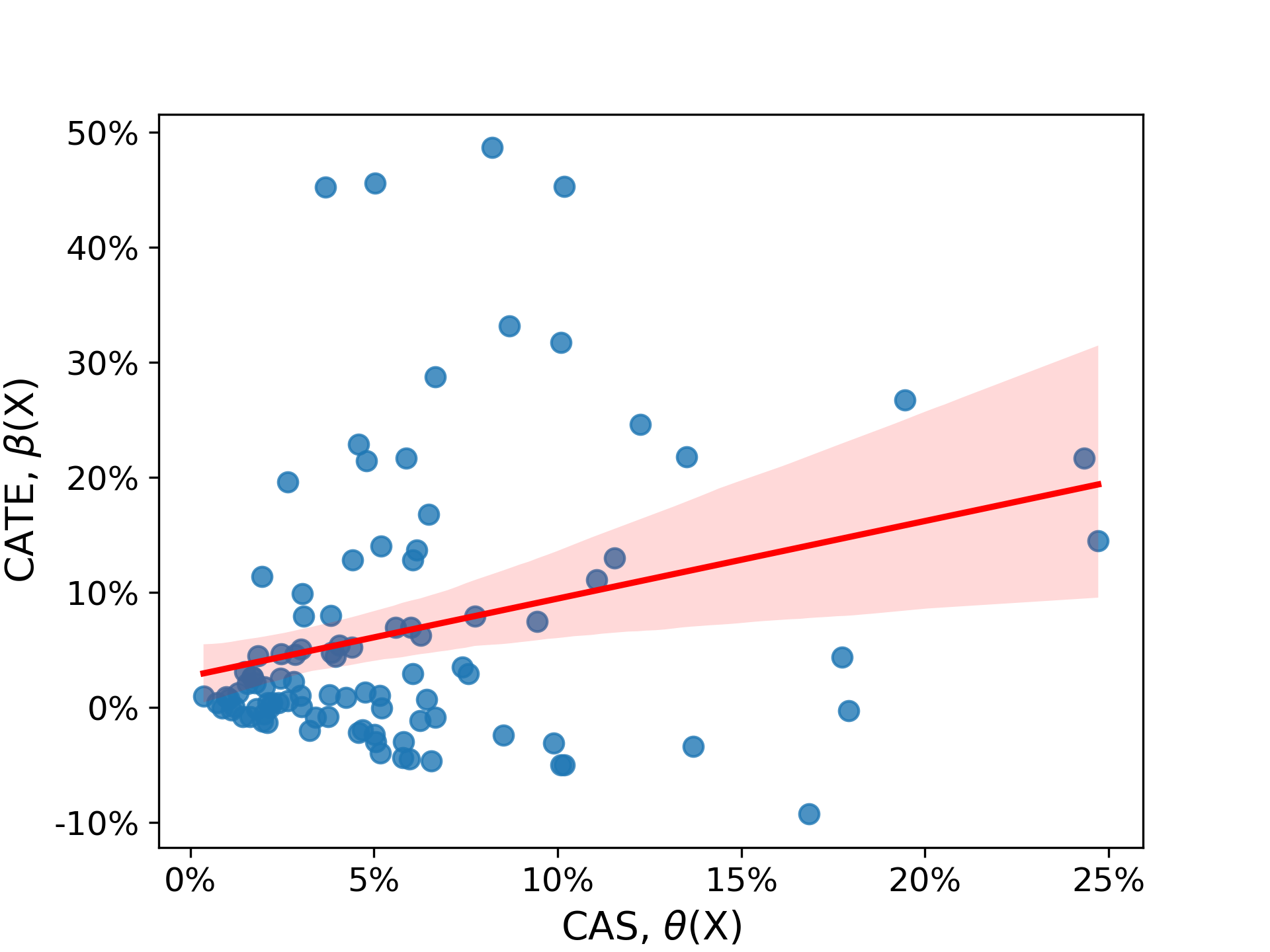
(d)

Figure 8: Relationship between the CAS and CATE in the absence of full latent mediation. The CAS remains highly correlated with the CATE when the nudge effect on the utility gain has little variance (Figures 8(a) and 8(c)) or when it is highly correlated with the utility gain without a nudge (Figures 8(a) and 8(b)).

In Figure 8, we depict the relationship between the CAS and the CATE under varying values of $\eta$ and $\rho$. As anticipated, a stronger correlation is observed between the CATE and the CAS when either $\eta$ is small (Figures 8(a) and 8(c)) or $\rho$ is large (Figures 8(a) and 8(b)). In these instances, the variability in $\mu(X)$ predominantly accounts for the heterogeneity in CATEs. Consequently, the CAS effectively ranks individuals based on their CATE, despite the lack of full latent mediation or a strictly valid EO interpretation.

4.2 Example 2: Latent mediators in surrogate outcomes

In our next example, we consider causal scores that correspond to predictions of the intervention’s effect on a proxy or surrogate outcome. Surrogate outcomes are often used to evaluate the effectiveness of interventions (Prentice, 1989, VanderWeele, 2013). For instance, in clinical trials, assessing the impact of a medical treatment on long-term outcomes like survival rate or quality of life may require years of observation (e.g., a five-year survival rate). Hence, it’s common to assess the intervention’s effect on surrogate outcomes as a substitute. For example, tumor shrinkage could stand in as a surrogate outcome for longer survival in drug trials for certain cancers.

Surrogate outcomes are also prevalent in marketing, where companies may be compelled to make decisions based on short-term proxies such as monthly revenue, despite their true interest lying in long-term outcomes like customer lifetime value. In the context of proactive churn management,  (Yang et al., 2020) discuss the use of surrogate short-term outcomes to estimate missing long-term outcomes. For a more details on the use of short-term proxies in estimating long-term causal effects across various domains, see Athey et al., (2016).

A rich history exists in the statistical evaluation of surrogate outcomes to predict the causal effect of interventions on another outcome of interest (Buyse et al., 2016). Commonly adopted criteria for assessing surrogate validity involve conceptualizing the surrogate outcome as a mediator for the treatment’s causal effect on the outcome of interest. The Prentice criteria, for example, require the surrogate outcome to fully mediate the effect of the treatment on the outcome of interest (Prentice, 1989). That is, the treatment leads to an improvement in the surrogate outcome, which in turn leads to an improvement in the outcome of interest. While these criteria don’t demand exact equivalence between causal scores and causal effects, they do align with full causal mediation, as illustrated in Figure 4(a): any ability to predict the effect of the treatment on the outcome of interest occurs exclusively through the surrogate outcome.

We aim to extend this perspective to a broader category of circumstances. Specifically, the concept of full latent mediation (depicted in Figure 5) proves valuable in describing situations where a shared, underlying factor (the latent mediator $L$) explains the effectiveness of the treatment on both the surrogate and the outcome of interest. In contrast to most existing frameworks on surrogate validity, full latent mediation implies that the surrogate does not need to be part of the causal pathway through which the treatment influences the outcome of interest. Instead, the (latent) mechanism through which the treatment impacts the surrogate is the same as the mechanism by which it would affect the outcome of interest.

In the subsequent discussion, we illustrate the application of causal scoring with surrogate outcomes in the healthcare domain. Consider the hypothetical scenario where a new and potentially fatal respiratory disease has emerged, and a policy maker must allocate a limited number of vaccines. While the policy maker knows that most patients would benefit from the vaccine, the scarcity of vaccines requires careful consideration. The policy maker wants to prioritize patients who would benefit the most from the vaccine in terms of reducing potential long-term health complications. However, the policy maker only has access to short-term survival data and lacks information on any long-term effects of the disease. Given the data limitations, the policy maker is considering using the effect of the vaccine on short-term survival as causal scores:

$$\begin{split}\theta(X)&=\mathbb{E}[\tilde{Y}\mid T=1,X]-\mathbb{E}[\tilde{Y}\mid T=0,X]\\ &=\mathbb{E}[\tilde{Y}^{1}-\tilde{Y}^{0}\mid X],\end{split}$$ (18)

where $\tilde{Y}=1$ if the patient survives in the short term, and $\tilde{Y}=0$ otherwise. In this context, $\tilde{Y}$ serves as a surrogate outcome for the long-term health measure $Y$—the primary outcome of interest, which encompasses both survival and potential long-term complications. The scoring variable is denoted as $S=\tilde{Y}^{1}-\tilde{Y}^{0}$, the effect on short-term survival (the surrogate outcome). Meanwhile, the causal effect of interest is $C=Y^{1}-Y^{0}$, the effect on long-term health.

The effect of the vaccine on long-term health is not fully mediated by short-term survival in this case, given the potential for the disease to lead to other chronic respiratory issues. Consequently, the causal scores do not meet conventional criteria for surrogate validity (e.g., Prentice criteria). However, an EO interpretation of the causal scores could be plausible. Let’s consider $X$ as a set of risk indicators conveying information about an individual’s susceptibility to the respiratory disease.

In this context, achieving full latent mediation entails that the individual’s susceptibility to the disease ($L$) is the only information captured by the risk indicators ($X$) that is pertinent in predicting both the vaccine’s effect on short-term survival ($S$) and long-term health ($C$). Furthermore, latent synchrony is met when a higher susceptibility to the disease always implies a more substantial impact of vaccines on both survival and long-term health. If these criteria are met, an EO interpretation is valid, so prioritizing individuals for whom the vaccines maximize short-term survival is the same as prioritizing individuals for whom the effect on long-term health is largest.

In short, an EO interpretation of the CAS based on a surrogate outcome (Equation (18)) is valid when the treatment effect on the surrogate outcome varies because of the same underlying mechanism causing variations in the treatment effect on the primary outcome of interest.

However, let’s examine the scenario where multiple latent mechanisms contribute to variations in treatment effects. For instance, the effectiveness of the vaccine on short-term survival and long-term health may not solely hinge on an individual’s susceptibility to the disease. Factors such as the likelihood of contracting the disease and the quality of home care if the disease is contracted could also play significant roles. In this context, it becomes evident that the full latent mediation assumption is violated, given the absence of a single latent mediator accounting for all the variability in effects. Nevertheless, we illustrate next that this violation is not necessarily catastrophic.

Given the presence of $k>1$ latent mediators $\{L_{1},...,L_{k}\}$ that depend on $X$, let the causal effects of vaccines on short-term survival ($S$) and long-term health ($C$) be represented as:

$$S=\tilde{Y}^{1}-\tilde{Y}^{0} =\sum_{i=1}^{k}\tilde{\gamma}_{i}L_{i}$$ (19)

$$C=Y^{1}-Y^{0} =\sum_{i=1}^{k}\gamma_{i}L_{i},$$ (20)

where $X$ exhibits predictive power over $S$ and $C$ due to its correlation with the $k$ latent mediators. Despite the absence of full latent mediation in this scenario, the question arises as to whether it remains reasonable to employ the surrogate outcome to infer the effect ordering of individuals. Two key considerations come into play to address this question.

The first consideration involves the relationship of each latent mediator to $C$ and $S$ in two regards. First, the qualitative relationship: do $\gamma_{i}$ and $\tilde{\gamma}_{i}$ share the same sign, indicating latent synchrony? Our next analysis focuses on cases where latent synchrony for each latent mediator can be reasonably assumed. Additionally, the relative strength of each mediator as a predictor also matters. If a mediator is a strong predictor for the effect on the surrogate outcome but negligibly predicts the effect on the primary outcome of interest, potential issues may arise. Conversely, if the mediator proves to be a strong (or weak) predictor for both effects, this concern is mitigated.

The second consideration is about how the latent mediators relate to each other. If mediators predictive of larger effects tend to be correlated, it is advantageous. When multiple latent mediators behave similarly (i.e., when an increase in one corresponds to increases in others), they act akin to a single latent mediator, thereby mitigating the severity of the violation of full latent mediation.

To illustrate the sensitivity of effect ordering to these considerations, let’s assume that $\gamma_{i}$ and $\tilde{\gamma}_{i}$ follow a joint distribution modeled as a multivariate log-normal distribution:

$$\gamma_{i} =e^{A},$$ (21)

$$\tilde{\gamma}_{i} =e^{B},$$ (22)

$$\begin{pmatrix}A\\ B\end{pmatrix} \sim\mathcal{N}\begin{bmatrix}\begin{pmatrix}0\\ 0\\ \end{pmatrix}\!\!,&\begin{pmatrix}1&\rho_{\gamma}\\ \rho_{\gamma}&1\end{pmatrix}\end{bmatrix}.$$ (23)

This formulation ensures latent synchrony for each mediator $L_{i}$ because both $\gamma_{i}$ and ${\tilde{\gamma}}_{i}$ are always positive. Moreover, $\rho_{\gamma}$ moderates the relative strength of mediator $L_{i}$ in predicting $C$ and $S$. A value close to 1 for $\rho_{\gamma}$ implies that when $L_{i}$ is a strong (weak) predictor of $C$, it tends to be a strong (weak) predictor of $S$ as well. Conversely, a value close to -1 implies the opposite: whenever $L_{i}$ is a strong (weak) predictor of $C$, it will tend to be a weak (strong) predictor of $S$.

Next, consider $\mu_{i}(X)=\mathbb{E}[L_{i}\mid X]$. To capture the interrelationships among latent mediators, assume the following multivariate normal distribution:

$$\begin{pmatrix}\mu_{1}(X)\\ \mu_{2}(X)\\ \vdots\\ \mu_{k}(X)\end{pmatrix}\sim\mathcal{N}\left[\begin{pmatrix}0\\ 0\\ \vdots\\ 0\end{pmatrix},\begin{pmatrix}1&\rho_{L}&\cdots&\rho_{L}\\ \rho_{L}&1&\cdots&\rho_{L}\\ \vdots&\vdots&\ddots&\vdots\\ \rho_{L}&\rho_{L}&\cdots&1\end{pmatrix}\right].$$ (24)

A higher value for $\rho_{L}$ indicates a tendency for these mediators to move similarly, mitigating the severity of the violation of full latent mediation. Conversely, lower values imply the opposite. Note that for this covariance matrix to be valid (positive semi-definite), we must have $\rho_{L}\geq-(k-1)^{-1}$.

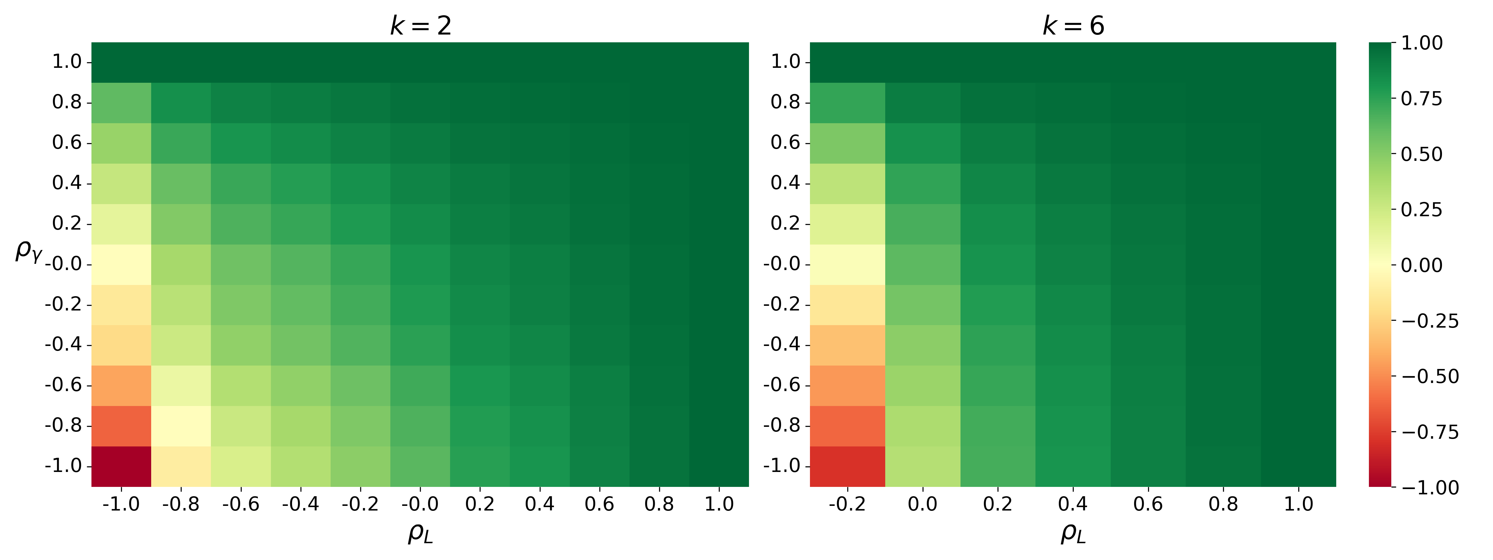
Figure 9: Correlation between CAS and CATE with $k=2$ and $k=6$ latent mediators. The correlation is stronger when mediators relate similarly to the CAS and the CATE (high $\rho_{\gamma}$) or highly correlate with each other (high $\rho_{L}$). This holds regardless of how many latent factors there are ($k$).

In Figure 9, we present heatmaps illustrating the correlation between the CAS and the CATE under varying values of $\rho_{L}$ and $\rho_{\gamma}$ for $k=2$ and $k=6$. As expected, there is a stronger correlation between the CATE and the CAS when either $\rho_{L}$ is high (indicating high correlation among mediators predictive of larger effects) or $\rho_{\gamma}$ is large (indicating that the mediators relate similarly to both the CAS and the CATE). Importantly, this holds irrespective of the value of $k$. In such cases, the CAS effectively ranks individuals based on their CATE, despite the lack of full latent mediation or a strictly valid EO interpretation.

4.3 Example 3: Self-selection in treatment assignment

In Section 4.1, we examined a scenario where we have complete control over an action (nudge) denoted as $T$. In the ensuing discussion, our focus shifts to a scenario where the action $T$ is a decision made by the agent—beyond our control—that causally influences an outcome of interest $Y$. For instance, $T$ could be the agent’s decision to pursue education, impacting their future wages (represented by $Y$). The objective is to delve deeper into understanding for which agents the causal effect of $T$ on $Y$ is largest (i.e., effect ordering). This insight could then guide decisions such as determining whom to subsidize or encourage in undertaking $T$.

We assume there is historical data on the agent’s attributes ($X$), their decision ($T$), and the outcome of interest ($Y$). The concern here is that agents choose the “treatment” (action $T=1$) on their own. This self-selection could lead to systematic differences between agents who choose $T=1$ (the treated) and those who opt for $T=0$ (the untreated), making it challenging to estimate the action’s effect by comparing the outcomes of the two groups of agents. In other words, the concern is that there could be some factors not capured in $X$ that are correlated with $Y$ and $T$ (i.e., confounders). However, careful consideration of why agents choose $T=1$ might help in understanding whether effect ordering can be achieved despite this data limitation.

In this example, we examine two potential CAS for determining the effect ordering: (a) the agent’s propensity for self-selection, and (b) the confounded estimate of the action’s effect. Let’s begin by exploring the agent’s propensity to self-select. We define this propensity as:

$$\theta(x)=\mathbb{P}[T=1\mid X=x]$$ (25)

Drawing from discrete choice modeling Train, (2009), we define the agent’s choice as:

$$T =\mathbf{1}\{U>0\},$$ (26)

where $U$ is the agent’s utility gain from choosing $T=1$ over $T=0$.

Based on the above, the CAS in Equation (25) has a valid EO interpretation if there is a full latent mediator, denoted as $L$, that applies to both $C$ and $U$ and satisfies latent synchrony. In simpler terms, the reason why the agent attributes in $X$ are informative about the magnitude of the causal effect is the same for why they are informative about the agent’s propensity to take action $T=1$.

Here are some possible candidates for such a latent mediator:

• $L=C$. Example: The agent’s utility of taking action $T=1$ is primarily driven by the action’s effect. Hence, the relationship between $X$ and $U$ is fully mediated by $C$.

• $L=U$. Example: The action’s effect depends mostly on the effort the agent puts, and the effort is proportional to the utility the agent gets from taking action $T=1$. Hence, the relationship between $X$ and $C$ is fully mediated by $U$.

• $L=Y$. Example: $T$ is an action complementary to $Y$, making both $U$ and $C$ contingent on $Y$. For instance, $T$ is subscribing to the gym and $Y$ is how much the agent exercises. Hence, the relationship between $X$ and both $U$ and $C$ is fully mediated by $Y$.

• $L$ is a latent factor that both moderates and confounds the effect. Example: $L$ is the agent’s capability, which determines their ability to carry out action $T=1$ and the action’s effectiveness.

The final bullet point highlights the key factor that enables causal scoring in this scenario: the presence of a latent variable that simultaneously acts as a moderator and a confounder. The moderator aspect establishes a correlation between the latent mediator and the effect, while the confounder aspect establishes a correlation between the latent mediator and the agent’s propensity for self-selection. Consequently, what makes this situation particularly intriguing is that the confounding, which might initially appear to complicate the task of effect ordering, actually provides predictive power. It serves as a signal of larger effects. Thus, unexpectedly, the very challenge that seemed to hinder effect ordering can be leveraged to recover the effect ordering.

Of course, it is important to acknowledge that the assumption of a single, overarching moderator and confounder is not insignificant. In real-world scenarios, multiple factors could contribute to individuals’ decision to take action $T=1$ and the effectiveness (or lack thereof) of that action. With regards to this limitation, we addressed in Section 4.2 the circumstances where the violation of full latent mediation does not necessarily have catastrophic consequences for effect ordering. The principles discussed in that section are also applicable here.

Considering that confounding can be beneficial when using the propensity to self-select as the CAS, it is worth exploring whether the same holds true when using (confounded) estimates of the effect as causal scores. To investigate this, we now shift our focus to examining the expected difference in $Y$ between treated and untreated groups as the CAS. This CAS was previously introduced in Equation (6) as follows:

$$\theta(x)=\mathbb{E}[Y\mid T=1,X=x]-\mathbb{E}[Y\mid T=0,X=x].$$

As outlined in Section 2, the ignorability assumption (Equation (7)) is crucial for interpreting the CAS as the CATE here. In the presence of confounders not fully accounted for by the features in $X$, which is the context of our scenario, the CAS won’t correspond to the CATE. Nevertheless, despite this limitation, an EO interpretation could still be reasonably justified.

This CAS corresponds to the expected value of the following scoring variable, which is also known as the transformed outcome (Athey and Imbens, 2016):

$$\begin{split}S=Y\frac{T-p}{p(1-p)},\\ p=\mathbb{P}[T=1\mid X].\end{split}$$ (27)

Discussing the effect ordering of such a complex scoring variable becomes challenging without carefully considering the DGP. In order to provide a more comprehensive understanding, we characterize the DGP by examining the agent’s outcome if they were to take action $T=0$ ($Y^{0}$), the effect of the action ($C$), and the utility gain ($U$) for choosing action $T=1$. So, the observed outcome corresponds to $Y=Y^{0}+\mathbf{1}\{U>0\}C$, and the individual components are:

$$Y^{0} =\zeta(X)+\epsilon_{y},$$ (28)

$$C =\beta(X)+\epsilon_{c},$$ (29)

$$U =\psi(X)+\epsilon_{u}$$ (30)

The terms $\epsilon_{y}$, $\epsilon_{c}$, and $\epsilon_{u}$ are unobserved variation not captured by $X$, so they are independent of $X$ and their expectation is 0.

We found that, under this DGP, full latent mediation and latent synchrony between $C$ and $U$ do not suffice to ensure that the confounded effect estimates can successfully recover the effect ordering. Therefore, we outline next four additional assumptions that, when satisfied, guarantee an EO interpretation of the CAS in the presence of unobserved confounding.

4.3.1 Assumption 1.

$\epsilon_{u}$ is linearly correlated to $\epsilon_{y}$ and $\epsilon_{c}$.

$$\mathbb{E}[\epsilon_{y}\mid\epsilon_{u}] =\alpha_{y}\epsilon_{u},$$ (31)

$$\mathbb{E}[\epsilon_{c}\mid\epsilon_{u}] =\alpha_{c}\epsilon_{u}.$$ (32)

The magnitude and direction of the unobserved confounding bias depend on $\alpha_{y}$ and $\alpha_{c}$. A positive (negative) $\alpha_{y}$ implies that the treated would experience a higher (lower) outcome $Y$ than the untreated if they do not take action $T=1$. A positive (negative) $\alpha_{c}$ implies that the effect $C$ of action $T=1$ is greater (smaller) on the treated than the untreated. Importantly, $\alpha_{y}$ and $\alpha_{c}$ represent sources of confounding that are not accounted for in $X$. Therefore, Assumption 1 is strictly weaker than ignorability, which requires $\alpha_{y}=0$ and $\alpha_{c}=0$.

To consider how $\alpha_{y}$ and $\alpha_{c}$ introduce bias, we decompose the CAS as follows:

$$\theta(X)=\mathbb{E}[C\mid T=1,X]+(\mathbb{E}[Y^{0}\mid T=1,X]-\mathbb{E}[Y^{0}\mid T=0,X])$$ (33)

The term on the left is the conditional average effect for treated individuals. We refer to this as the CATT (Conditional Average Treatment effect on the Treated). The term inside the parentheses represents the baseline bias, indicating the difference in the expected outcome in the absence of treatment between those in the treatment group and those in the control group.

Given Assumption 1, $U$ is a full latent mediator for the baseline bias, meaning that all variation in the baseline bias given $X$ is captured by $U$ through $\psi(X)$ (proof in Appendix E):

$$\mathbb{E}[Y^{0}\mid T=1,X]-\mathbb{E}[Y^{0}\mid T=0,X]=\alpha_{y}(\mathbb{E}[\epsilon_{u}\mid\epsilon_{u}>-\psi(X)]-\mathbb{E}[\epsilon_{u}\mid\epsilon_{u}\leq-\psi(X)]).$$ (34)

Similarly, given Assumption 1, the CATT corresponds to (proof in Appendix E):

$$\mathbb{E}[C\mid T=1,X]=\beta(X)+\alpha_{c}\mathbb{E}[\epsilon_{u}\mid\epsilon_{u}>-\psi(X)].$$ (35)

The left term ($\beta$) is the CATE, while the right term is the differential effect bias—the difference between the CATE for the treated and the CATE for both the treated and untreated. This latter term depends exclusively on $U$, so the relationship between $X$ and the confounding bias, encompassing both differential effect bias and baseline bias, is fully mediated by $U$.

Therefore, in the presence of full latent mediation for $C$ and $U$, Assumption 1 implies full latent mediation for $C$ and the CAS, as variations in the latent mediator completely account for variations in the CATE and the confounding bias. What remains to be determined is whether latent synchrony is satisfied. Latent synchrony is met for the CAS if both the CATT and the baseline bias are strictly increasing in $\psi$. The next three assumptions are used to establish latent synchrony.

4.3.2 Assumption 2.

$T$ follows a probit model.

$$\epsilon_{u}\sim\mathcal{N}(0,1),$$ (36)

We use this assumption to derive how the CATT and the baseline bias change as $\psi$ increases. While we assert that our conclusions are likely robust to the normality assumption of $\epsilon_{u}$, we are unable to provide conclusive evidence due to the substantial complexity involved in the analytical derivations. We think that the results should hold under the weaker condition that $\epsilon_{u}$ follows a unimodal symmetric distribution, but a formal proof remains elusive. Therefore, we encourage future research on the generalizability of our results beyond this parametric assumption.

4.3.3 Assumption 3.

The baseline bias is increasing in $\psi$, which happens if:

$$\psi(X)\alpha_{y}>0,\forall X.$$ (37)

The proof is in Appendix E. This is equivalent to assuming that:

• There is positive baseline bias ($\alpha_{y}>0$) and $\mathbb{P}[T=1\mid X]>50\%$ for all agents,

• Or there is negative baseline bias ($\alpha_{y}<0$) and $\mathbb{P}[T=1\mid X]<50\%$ for all agents.

Under this assumption, the baseline bias is larger for agents who are more likely to take action $T=1$. While the value of $\alpha_{y}$ will generally be unknown, a clear correlation between baseline outcomes and treatment decisions should be indicative of its sign. For example, if agents tend to choose action $T=1$ to prevent an undesirable outcome in $Y$ we should expect $\alpha_{y}<0$. Alternatively, if the action $T=1$ complements $Y$ in a way that makes the action more favorable when $Y$ is high, we should expect $\alpha_{y}>0$. The distribution of $\psi(X)$ can be estimated from historical data.

4.3.4 Assumption 4.

The CATT is increasing in $\psi$, which happens if:

$$\frac{d\beta}{d\psi} \geq\alpha_{c}(1-\tilde{p}(X)),\forall X,$$ (38)

and $\beta$ is a differentiable function of $\psi$.

The proof is in Appendix E. Here, $\tilde{p}(X)$ is a value that scales with the probability of treatment $p=\mathbb{P}[T=1\mid X]$, converging to 1 as $p$ approaches 1 and to 0 as $p$ approaches 0. Under Assumption 2, $\tilde{p}(X)=\mathrm{Var}[\epsilon_{u}\mid T=1,X]$. The quantity $\alpha_{c}$ captures the direction and magnitude of the differential effect bias. Finally, $d\beta/d\psi$ represents how the CATE changes with the expected utility gain.

We reason about Equation (38) under the assumption that there is full latent mediation and latent synchrony between $C$ and $U$. If this is the case, then $d\beta/d\psi$ is positive, and Assumption 4 holds if the differential effect bias is negative ($\alpha_{c}<0$).

Assumption 4 also holds when the correlation between $C$ and $U$ captured by $X$ is at least as strong as the correlation between $\epsilon_{c}$ and $\epsilon_{u}$, so that $d\beta/d\psi\geq\alpha_{c}$. This will always be the case if the relationship between $C$ and $U$ is linear because then $d\beta/d\psi=\alpha_{c}$. For cases where $C$ and $U$ have a non-linear relationship and $\alpha_{c}>0$, Assumption 4 remains plausible if the latent mediator is significantly more strongly associated with causal effects than with the agents’ utility of taking action $T=1$. This is because $d\beta/d\psi$ can be broken down into the ratio of $d\beta/d\mu$ and $d\psi/d\mu$. These two quantities represent the latent mediator’s connection with effects and the agents’ utility gain, respectively. Thus, the inequality in Equation (38) is more likely to hold when $d\beta/d\mu$ is substantially greater than $d\psi/d\mu$.

Finally, Assumption 4 is also more credible when the probability of treatment tends to be large for most individuals ($\tilde{p}$ is large). The rationale behind this is that the CATT is a biased estimate of the CATE only for untreated individuals. Therefore, if the fraction of untreated individuals is relatively small, the differential effect bias is smaller and less likely to disrupt the effect ordering.

In scenarios where individuals have small values of $\tilde{p}$, the CATT becomes less likely to be strictly increasing in $\psi$; however, even if the effect ordering is disrupted because of this, the CAS may still be valuable for distinguishing between individuals with high and low CATEs, preserving an EC interpretation. The latent synchrony between $C$ and $U$ implies that individuals with smaller expected utility gains (i.e., smaller values for $\tilde{p}$) also have smaller CATEs. Consequently, even if the effect ordering is disrupted for individuals with smaller values for $\tilde{p}$, it may happen only for individuals with relatively smaller CATEs. Figure 10 shows an example of this.

Figure 10: CATT and CATE as a function of the propensity to self-select when Assumption 4 is violated for some individuals. We cannot recover the effect ordering for everyone in this example, but the CAS has a valid EC interpretation if we want to identify individuals with a CATE larger than 6.

4.3.5 Establishing effect ordering.

If Assumptions 1 to 4 are satisfied, along with full latent mediation and latent synchrony for $C$ and $U$, then the CAS based on confounded effect estimates can recover the effect ordering of individuals despite the presence of confounding (proof in Appendix E). However, considering the large number of assumptions, one might question their utility for establishing effect ordering in the presence of unobserved confounding.

It’s essential to recognize that this research focuses on addressing scenarios where obtaining unconfounded data is practically impossible. In this example, agent actions cannot be randomized, and accounting for all confounding factors affecting both actions and outcomes is unfeasible. The prevailing academic stance often suggests refraining from attributing causation to statistical estimates in such scenarios. However, this perspective may not be beneficial for decision makers seeking guidance on whom to encourage or subsidize action $T=1$, as it essentially involves disregarding historical data and making decisions without any data at all. The assumptions we propose provide a structured framework for decision makers to assess whether using the problematic data to inform their decisions is a better alternative.

In this scenario, two assumptions play a critical role: the full latent mediation and latent synchrony of $C$ and $U$. To evaluate the sensitivity of the causal scoring to violations of these assumptions, similar sensitivity analyses as those employed in Sections 4.1 and 4.2 could be used.

If we are willing to assume that most confounders are also moderators, then using the propensity to self-select for effect ordering is probably a better alternative than giving up on using the historical data at all. Our analysis suggests that using the confounded estimates as the CAS could also be a reasonable alternative, but it would require making additional assumptions about the DGP.

It may then appear that the propensity to self-select is a strictly superior candidate for the CAS compared to confounded estimates of the effect, as the latter requires more assumptions to establish a valid EO interpretation. However, this is not necessarily the case in practice because it overlooks the statistical challenge of estimating the causal scores.

So far, we have focused on whether the target of the statistical estimation (the CAS) can rank individuals in the same way as the CATE, without considering the challenge of actually estimating the CAS. This is an important point because, in practice, selecting the confounded effect estimates as the CAS instead of the propensity to self-select might be the right choice due to statistical efficiency. In the next section, we cover the estimation of the CAS and revisit this discussion.

5 Estimation of Causal Scores

In the past examples, we showed that relaxing the requirements of causal interpretations allows us to satisfy them in a broader range of settings. However, it is important to avoid the misconception that alternative causal interpretations such as EC or EO are only valuable when an EE interpretation is not possible. We discuss next how these alternative causal interpretations can also be valuable to guide the statistical modeling of the causal scores, including in cases where one could potentially estimate causal scores with a valid EE interpretation.

Recall that the CAS corresponds to an estimand, not an estimate. In practice, decisions are made with an estimated model $\hat{\theta}$, which we formulate as:

$$\begin{split}\hat{\theta}(x)&=\beta(x)+\xi,\\ \alpha(x)&=\mathbb{E}[\xi\mid X=x],\end{split}$$ (39)

where $\xi$ is a random variable that represents estimation error, and $\alpha(x)$ corresponds to bias in the estimation that could come from a mismatch between the CAS and the CATE or from incorrect parametric assumptions in the estimation procedure. The deviations in $\xi$ represent variance in the estimation procedure due to randomness in the data sample.

When the aim of the causal estimation is an EE interpretation, it is desirable to have a model with small deviations in $\xi$ and a value close to zero for $\alpha(x)$. In other words, reducing both bias and variance is crucial for improving the accuracy of the causal estimation. However, achieving both simultaneously is often unfeasible because decreasing bias often leads to an increase in variance, so managing the bias–variance trade-off is important. For example, the use of double/debiased ML to reduce confounding bias can result in substantially worse effect estimation than simpler methods due to increased variance (Gordon et al., 2023).

In general, evaluating a causal model requires careful consideration of the purpose for which the model estimates will be used. In the context of decision-making processes, the resulting estimates are often employed for effect ordering or effect classification, making an EO or EC causal interpretation more relevant than an EE interpretation. Recent studies have shown that bias and variance have different implications for EC and EE and that bias can actually be beneficial for EC by reducing errors caused by variance (Fernández-Loría et al., 2022, Fernández-Loría and Provost, 2019, Fernández-Loría and Provost, 2022a ). The main implication is that optimizing the bias–variance trade-off for EC rather than EE can improve decision-making performance.

In this section, we extend these prior results to consider cases where the purpose of the estimates is effect ordering. We use the Kendall rank correlation coefficient (Kendall, 1938) to measure the estimated model’s ability to order individuals according to their effects. Let $x_{i}$ be the feature values for the individual with the $i$-th largest CATE. Assuming there are $n$ individuals to be ordered, the rank correlation ($\kappa$) between the CATE and the estimated model is:

$$\begin{split}\kappa&=\frac{2}{n(n-1)}\sum_{i<j}\text{sgn}(\beta(x_{i})-\beta(x_{j}))\text{sgn}(\hat{\theta}(x_{i})-\hat{\theta}(x_{j}))\\ &=\frac{2}{n(n-1)}\sum_{i<j}\text{sgn}(\hat{\theta}(x_{i})-\hat{\theta}(x_{j})).\end{split}$$ (40)

Note that $-1\leq\kappa\leq 1$. The estimated model preserves the effect order only when $\kappa=1$. However, in most practical settings, the estimates will not perfectly preserve the ranking because of bias and variance. Therefore, we use the expected rank correlation next to assess how bias and variance can affect the estimation of the effect ordering.

Theorem 3.

The expected rank correlation between the CATEs and the estimated model is:

$$\mathbb{E}[\kappa]=\left(\frac{4}{n(n-1)}\sum_{i<j}\mathbb{P}[\xi_{\Delta}<\beta_{\Delta}+\alpha_{\Delta}]\right)-1,$$ (41)

where

$$\beta_{\Delta} =\beta(x_{i})-\beta(x_{j})>0,$$

$$\alpha_{\Delta} =\alpha(x_{i})-\alpha(x_{j}),$$

$$\xi_{\Delta} =(\xi\mid X=x_{i})-(\xi\mid X=x_{j})-\alpha_{\Delta},$$

$$\mathbb{E}[\xi_{\Delta}] =0.$$

The proof is in Appendix F. In Equation (41), $\beta_{\Delta}$ is the rate of change of the CATE, $\alpha_{\Delta}$ is the rate of change of the bias, and $\xi_{\Delta}$ is a random variable centered around 0 that captures variance in the estimated difference between causal scores. Theorem 3 shows that the expected rank correlation improves when $\alpha_{\Delta}>0$ and decreases when $\alpha_{\Delta}<0$. In other words, the quality of the effect ordering improves when the rate of change in the bias ($\alpha_{\Delta}$) is positive, and the larger the rate of change, the better. As a result, the bias helps to infer the effect ordering when the estimates for individuals with larger effects have larger positive bias or a smaller negative bias.

This is consistent with studies showing that confounded models (Fernández-Loría and Provost, 2019) and non-causal models (Fernández-Loría and Provost, 2022a ) can lead to better treatment decisions than unconfounded CATE models. This occurs when the bias cancels errors due to variance by pushing estimates in the “right direction” (Friedman, 1997). In Equation (41), this means pushing causal scores farther away from the causal scores of individuals with smaller CATEs.

We discuss next how bias can help as a result of full latent mediation, as illustrated in Figure 5. Specifically, if the latent mediator has a stronger correlation with the scoring variable than with the causal effect, then the bias will improve the effect ordering.

Theorem 4.

Let $\theta(X)=\mathbb{E}[\hat{\theta}(X)]$. Assume full latent mediation, which implies Lemma 1 is met. Let $g_{\Delta}=g(\mu(x_{i}))-g(\mu(x_{j}))$ and $h_{\Delta}=h(\mu(x_{i}))-h(\mu(x_{j}))$ represent the change in $g$ and $h$ for given points $x_{i}$ and $x_{j}$. Then, the bias improves the expected rank correlation of those points (i.e., $\alpha_{\Delta}>0$) if and only if:

$$\frac{h_{\Delta}}{g_{\Delta}}>1.$$ (42)

The proof for this statement can be found in Appendix G. Equation (42) provides a more stringent condition than latent synchrony (Equation (13)). In addition to requiring that the causal effects and causal scores exhibit the same qualitative relationship with the latent mediator (i.e., both numerator and denominator have the same sign), Equation (42) also requires a stronger association between the causal scores and the latent mediator than the causal effects and the latent mediator (i.e., the numerator has a greater absolute value than the denominator).

If the ratio in Equation (42) is greater than 1, the bias introduced by the causal scores improves the rank estimation by reducing variance errors. Conversely, if the ratio is lower than 1, the bias has a negative impact on the estimation by increasing errors due to variance (when the ratio is between 0 and 1) or violating the latent synchrony assumption (when the ratio is less than 0).

To provide additional context for this result, let’s revisit the nudging example discussed in Section 4.1. We considered the agent’s utility in making the desired choice without any nudge as a latent mediator that explains the variation in nudge effects. Essentially, the CATE increases as the agent’s utility gets closer to the decision threshold. However, a challenge arises when large variations in utility only lead to small changes in the CATE. For instance, Figure 6 shows that a change in the expected utility from -1 to 0 reflects only a small change in the nudge effect from 10% to 12%, whereas the CAS changes from 27% to 50%.

This observation implies that estimating the effect ordering from the CAS is easier because the signal-to-noise ratio is higher. In fact, the bias is an integral part of the signal: the effectiveness of a nudge depends on how close the agent is to tipping over the decision threshold, and predictions about the agent’s decision without the nudge are more strongly correlated with that proximity than the expected effect of the nudge itself. Consequently, targeting nudges based on predicted baseline outcomes can be more effective than targeting them based on the expected effect of the nudge, even if the ultimate goal is to maximize the effect of the nudges. This finding aligns with empirical evidence presented in (Athey et al., 2023).

Returning to our discussion on comparing different approaches for causal scoring in the presence of confounding (Section 4.3.5), it is crucial to assess not only the conditions that establish a valid EO interpretation for each approach but also the strength of the association between the approaches and the latent mediator that connects them to the CATE. For instance, if the latent mediator, acting as both a confounder and a moderator, exhibits a stronger correlation with the baseline outcome than the propensity of agents to self-select, then the confounded estimate of the effect may be a more suitable alternative for the CAS. This is because the baseline bias could display a stronger correlation with the latent mediator than the propensity for self-selection. As a result, the baseline bias itself could be a valuable signal for effect ordering.

Another important consideration is the size of the data. There are many cases where decision makers may have little or no data for estimating CATEs without bias, but they may have a large amount of data for estimating causal scores that cannot be given an EE interpretation. We consider next the implications of large data for effect ordering.

Corollary 1.

If the CAS has a valid EO interpretation, then $\kappa$ converges in probability to $1$ as the size of the training data increases.

The proof can be found in Appendix H. Corollary 1 indicates that when the CAS has a valid EO interpretation, any adverse effect of the bias on effect ordering can be rectified by utilizing more training data. Therefore, even if the bias negatively affects the ranking estimation, its impact can become inconsequential with a sufficiently large data set. Thus, a CAS with only a valid EO interpretation that was estimated using a large data set could yield better results for effect ordering than a CAS with a valid EE interpretation estimated using a smaller data set.

6 Empirical Example

We next provide an empirical advertising example that illustrates how causal scores that are problematic for EE can be valuable for EO and EC.

6.1 Application Setting

The data in our example were assembled by Criteo (an advertising platform) after running a controlled experiment in which advertising was randomly targeted to a large sample of online consumers. This data set was released to benchmark methods for uplift modeling (Diemert Eustache, Betlei Artem et al., 2018). It measures two outcome variables: visits and conversions. The data consist of 13,979,592 rows, each one representing a user with 11 features, a treatment indicator for the ad, and the labels (visits and conversions). The treatment rate is 85%, the average visit rate is 4.7%, the average conversion rate is 0.3%, the average treatment effect (ATE) on the visit rate is 1%, and the ATE on the conversion rate is 0.1%. In our example, the causal effect of interest is the ad effect on conversions.

To evaluate various formulations of the CAS, we split the Criteo data into a training set with 10 million rows and a test set with the remaining rows. The CAS formulations we consider are:

1. CATE on conversion. This approach assumes the decision maker can and is willing to run a large-scale controlled experiment to collect unconfounded training data. Another assumption is that the outcome of interest (conversions) can be properly measured.

2. CATE on visits: Having limited data, or even no data, on the true outcome of interest is a common limitation in advertising even when experimentation is feasible, so advertisers often use auxiliary data to identify a suitable alternative (proxy) target variable. Website visits have been shown to be a good proxy for conversions (Dalessandro et al., 2015).

3. Conversion rate. The most common approach in targeted advertising is to target ads based on predicted conversion rates, not causal effects. One of the main reasons is the difficulty of running controlled experiments: they can be prohibitively expensive (Gordon et al., 2022) or even technically impossible to implement on many ad platforms (Johnson, 2022). Conversion rates are often correlated with causal effects (Radcliffe and Surry, 2011).

We use gradient boosting based on decision trees to estimate all the CAS formulations. We estimate the CATEs by regressing the transformed outcome as defined in Athey and Imbens, (2019). Other approaches for CATE estimation work similarly well in this data set (see Appendix I).

6.2 Evaluation Measures

Yadlowsky et al., (2021) propose an evaluation framework to assess the extent to which individuals who are highly ranked by a causal scoring model are more responsive to treatment than the average individual. They also show that several common evaluation metrics considered in the literature to assess treatment assignment performance are in fact special cases of their framework. We use two of these special cases to evaluate the EO and EC performance of the causal scoring models; other measures might be more appropriate depending on the context.

We measure EO performance with the area under the Qini curve (AUQC), which evaluates how good a model is at ranking individuals according to their CATEs (Radcliffe, 2007). Qini curves are used in uplift modeling to depict the cumulative incremental gain in the outcome (conversions in our example) that is achieved in a test set when the top percent of individuals with the largest scores are treated. The curve is constructed by ranking customers according to their predicted scores on the horizontal axis, and the vertical axis plots the cumulative number of conversions in the treatment group (scaled by the treatment group’s size) minus the cumulative number of purchases in the control group (scaled by the control group’s size).

Qini curves can be built using A/B test data, so practitioners who have access to experimental data can use this tool to visualize the performance of any causal scoring model. A model’s AUQC is the model’s area under the curve divided by the maximum area that could possibly be under the curve. Therefore, the AUQC summarizes the curve information in one number that is larger when the model is better at ranking individuals according to their causal effects. Figure 11 shows an example of a model’s Qini curve and its AUQC.

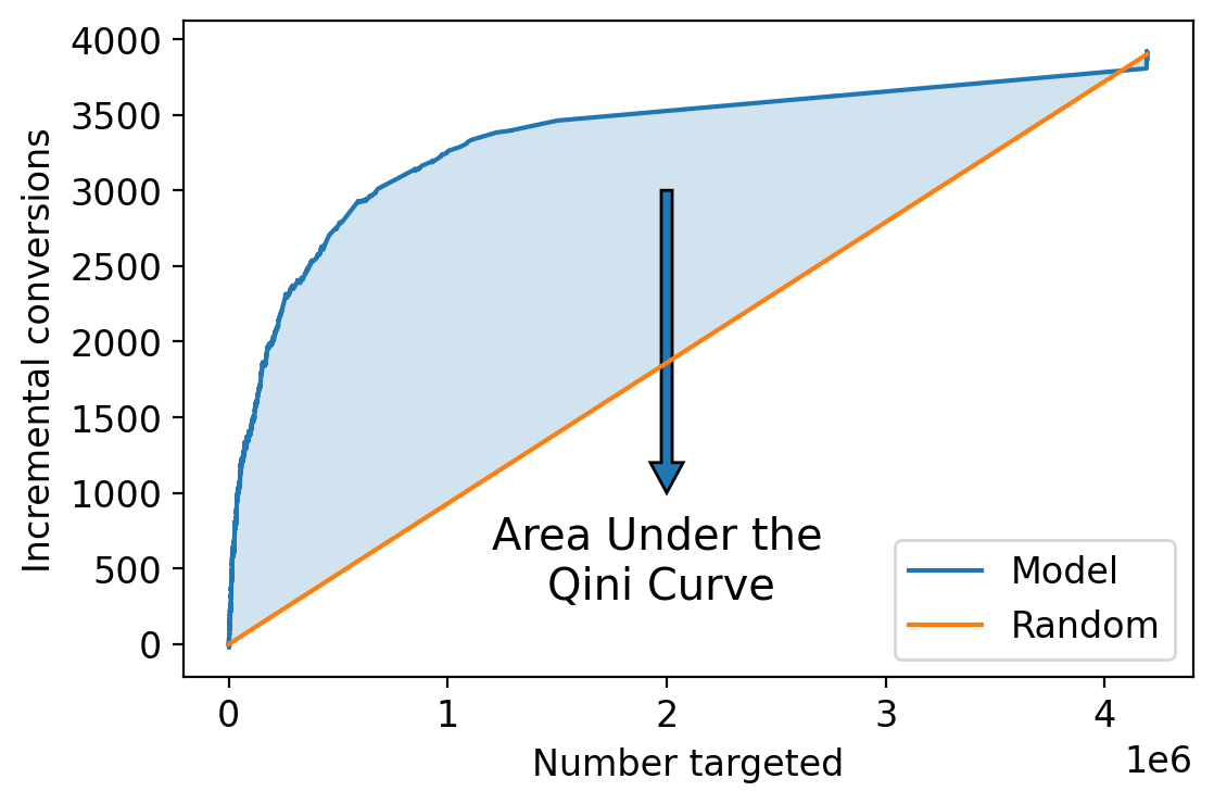
Figure 11: Example of a Qini curve (blue line). A larger area under the Qini curve (AUQC) means that the model is better at ranking individuals according to their causal effects.

To measure EC performance, we use the average causal effect for the top 10% of individuals with the largest predicted causal scores in the test set—the Top 10% Uplift. The assumption here is that the decision maker has a large enough marketing budget to target 10% of all potential targets with the ad. So, a larger Top 10% Uplift implies that the model is better at finding the top 10% individuals with the largest causal effects, which is an EC task.

6.3 Results

Our evaluation is based on the average of 100 different splits of the data into a training set and a test set. The results are reported in Figure 12.

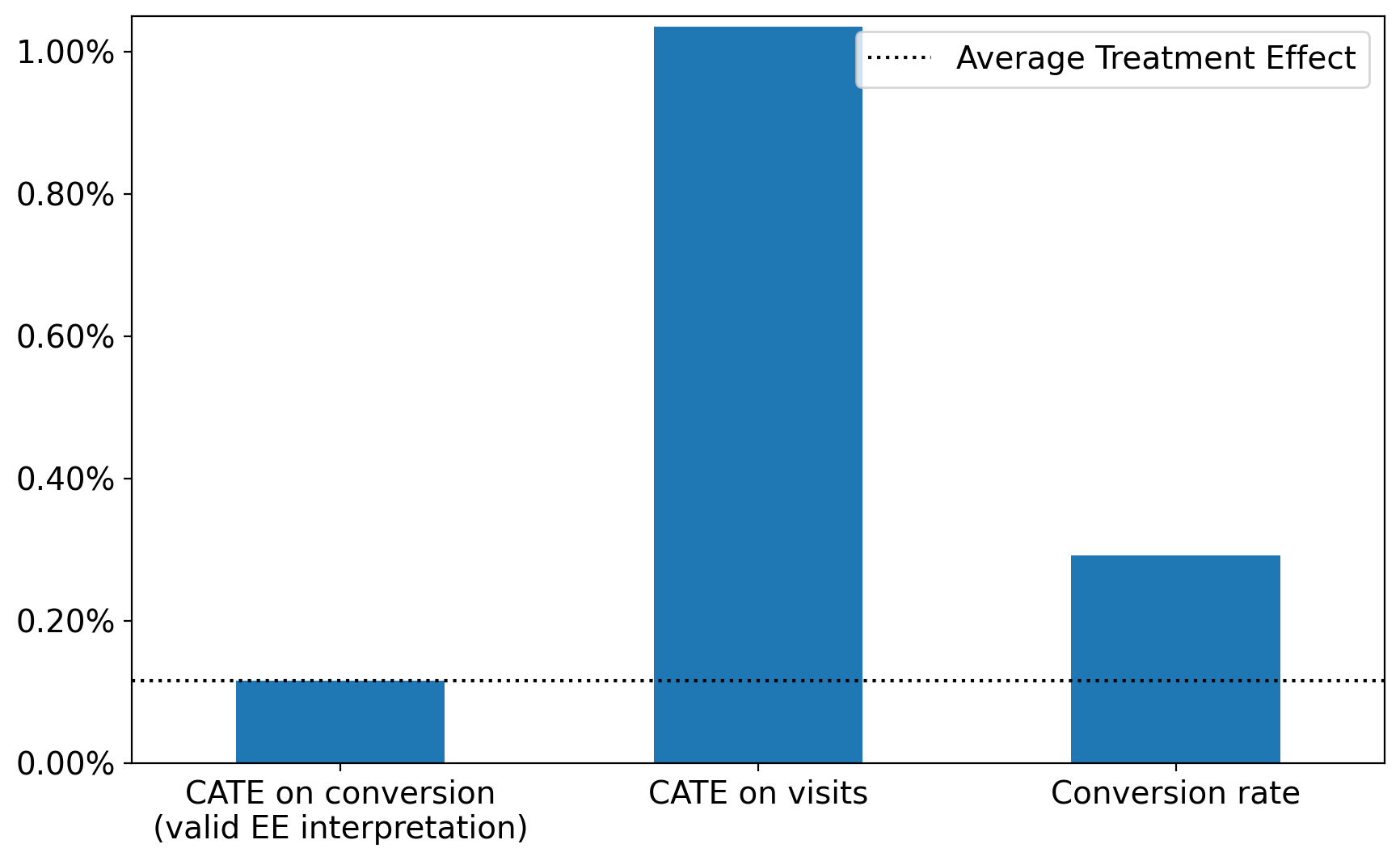
(a)

(b)

(c)

(d)

Figure 12: Comparison of causal scoring models. Only the CATE-on-conversion model performs well at effect estimation (Figure 12(a)), but all models perform similarly well at effect classification (Figure 12(b)) and effect ordering (Figures 12(c) and 12(d)). In fact, the conversion rate model performs best for effect ordering and effect classification, despite not being useful for effect estimation.

Figure 12(a) shows that the causal scoring models that are based on a proxy (“CATE on visits”) and a non-causal quantity (“Conversion rate”) are clearly inappropriate for effect estimation; the average causal score of these models is substantially larger than the average treatment effect represented as a dotted line in the figure. However, the other figures show that all the causal scoring models perform similarly well at finding the top 10% individuals with the largest causal effects (Figure 12(b)) and ranking individuals according to their causal effects (Figures 12(c) and 12(d)). Figure 12(b) shows that even the causal scoring model that performs worse (“CATE on visits”) can identify individuals for whom the treatment effect on conversions is about seven times larger than average (the dotted line in Figure 12(b) represents the average). This is a remarkable result considering that only one of the three models can be given an EE interpretation.

The results also demonstrate that the conversion rate model outperforms the CATE-on-conversion model, which can be explained by our theoretical results in Section 5. In that section, we highlighted the potential benefit of bias for effect ordering and classification, as it could help decrease errors due to variance. This outcome is particularly surprising in this case considering that the CATE-on-conversion model was trained using a substantial data set of 10 million observations. The performance gap would be even more pronounced in situations where obtaining large-scale experimental data is impractical or cost prohibitive.

To provide further support for our claim that the superior performance of the conversion rate model is attributed to the bias, we present evidence in Figure 13. This bar chart categorizes the observations in the test set into quintiles based on their predicted conversion rates. For example, the segment labeled “0%–20%” represents the 20% of observations in the test set with the lowest predicted conversion rates. The blue bars represent the estimated average effect within the quintile, which we estimate with the test data as the difference between the average outcomes of the treated and untreated observations in that particular quintile. The orange bars indicate the average bias per quintile, which is the difference between the average conversion rate (causal score) and the average causal effect within that quintile.

Notably, the chart reveals that both the bias and the causal effect become more pronounced as predicted conversions increase, indicating a correlation between the bias and the effect sizes. Our theoretical results in Section 5 showed that in such cases, the bias enhances the accuracy of the statistical estimation by reducing errors due to variance. This explains why predicted conversion rates serve as better causal scores than the actual effect estimates in this example.

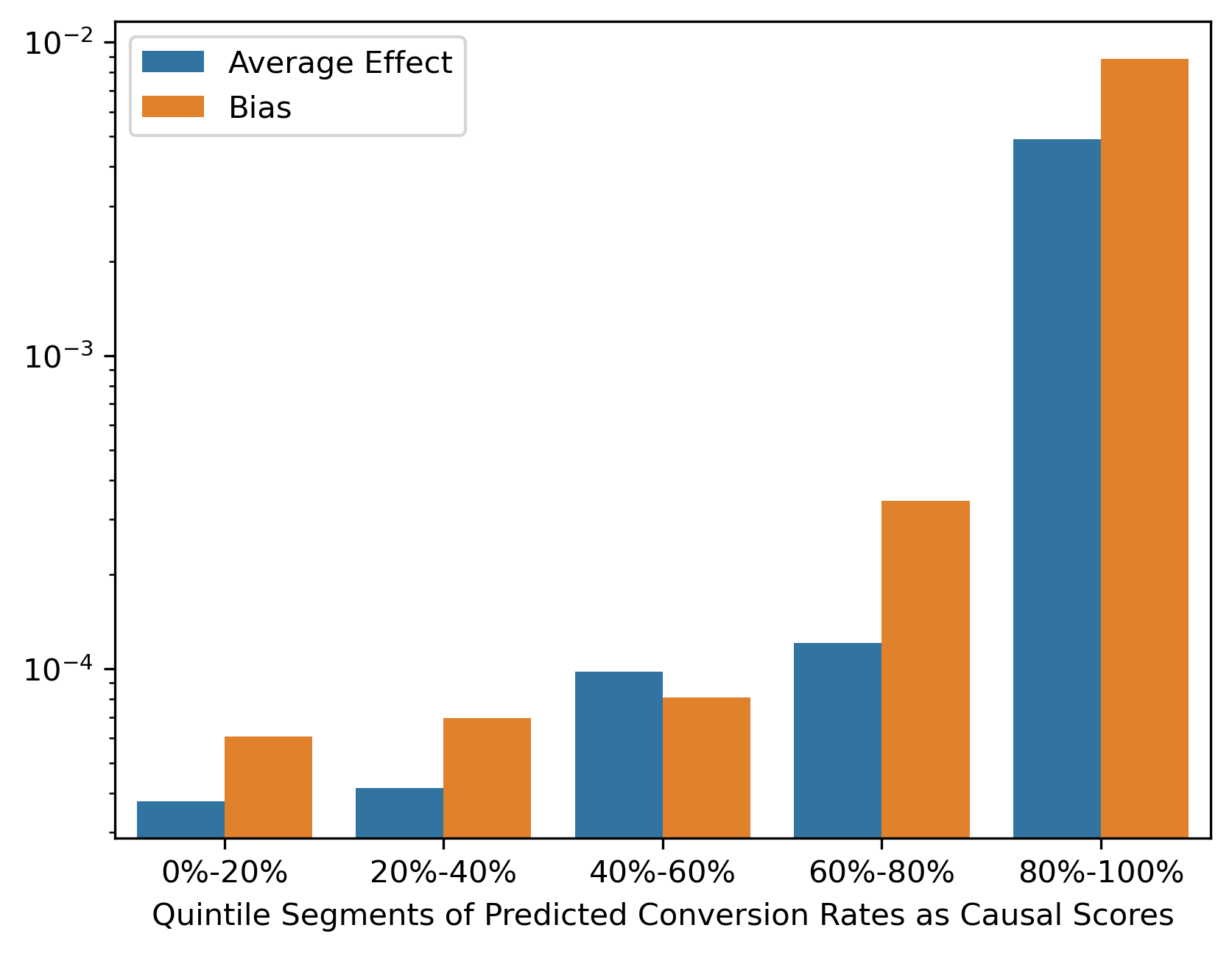
Figure 13: Bias by quintile of predicted conversion rates as causal scores. Effect sizes and bias are correlated, which benefits effect ordering by decreasing errors due to variance.

However, it is important to acknowledge that while these empirical results provide suggestive evidence for a valid effect ordering (EO) interpretation of conversions as a scoring variable, they do not guarantee it. Instead, they simply show that the estimated conversion rate model performs better at effect ordering and classification than the estimated CATE-on-conversion model. This performance gap arises from the bias-variance trade-off inherent in the conversion rate model, which leads to more accurate effect ordering and classification than the bias–variance trade-off of the CATE-on-conversion model. It is worth noting that with a larger volume of data, the CATE-on-conversion model should theoretically catch up with the conversion rate model and potentially surpass it if conversions do not align with a valid EO interpretation.

7 Discussion

In the introduction of this research paper, we initially posed the overarching question that served as the driving force behind our study: “When can we use ‘incorrect’ causal estimates for the purposes of causal decision making?” Our main contribution is reframing the formulation of this question. Rather than regarding causal estimates as inherently invalid when they fail to align with causal effects, we introduced the concept of causal scoring as a valuable tool for describing alternative causal interpretations that may still be valid for these “incorrect” estimates. Thus, in response to the original question, we can leverage imperfect causal estimates— estimates that may not directly correspond to causal effects—when we can endow them with causal interpretations that offer valuable insights for decision making.

7.1 Other Decision-Making Contexts

Within our causal scoring framework, we put forth two alternative causal interpretations: effect ordering and effect classification. While the framework has the flexibility to incorporate other interpretations, we specifically introduced these two because they align with prevalent applications of CATE estimation in decision-making contexts. More specifically, we examine scenarios that involve allocating treatments to individuals with a “large enough” effect (effect classification) or where decision makers operate within resource limitations and seek to prioritize individuals who are most likely to benefit from interventions (effect ordering).

These scenarios align closely with several practical applications of causal estimation for decision making, including customer retention (Ascarza et al., 2018), subsidy allocation (Bhattacharya and Dupas, 2012), and personalized medicine (Kent et al., 2020). These are applications where acquiring the appropriate data for effect estimation is difficult.

In the context of clinical decision making, for example, Kent et al., (2020) note that “although observational studies seem to offer many important advantages over conventional RCTs for more refined analyses (that is, enhanced statistical power and patient heterogeneity), when these data may be sufficiently debiased for reliable determination of treatment effects or [heterogeneous treatment effects] is not well understood. [We] identified these issues as high research priorities.” We contribute to this research priority by proposing a framework that helps determine when data can be considered “sufficiently debiased,” depending on the causal interpretation we need to attribute to the statistical estimates.

Of course, in practice, the usefulness of these alternative interpretations will ultimately depend on the specific decision-making context. For example, EC interpretations depend critically on the decision threshold $\tilde{\tau}$. In resource-constrained environments where we only care about identifying the top $k$ individuals with the largest predicted effects, setting an appropriate value for $\tilde{\tau}$ is trivial.

However, challenges arise when the decision maker wants to use the causal estimates to decide whether intervening is worthwhile. For example, the decision maker may want to intervene only if the causal effect is large enough to offset the cost of the intervention. In such cases, it can be difficult to set an appropriate $\tilde{\tau}$. Fortunately, we can mitigate this challenge with a profit curve (Provost and Fawcett, 2013) if we have access to at least some unconfounded data, even if it is only a limited amount. With an unconfounded test set, the expected causal impact of a treatment allocation policy implemented with $\hat{\theta}$ and $\tilde{\tau}$ can be estimated as:

$$n\times\mathbb{P}[D=1]\times(\mathbb{E}[Y\mid T=1,D=1]-\mathbb{E}[Y\mid T=0,D=1]),$$ (43)

where $n$ is the number of potential candidates for the treatment, and $D=\mathbf{1}\{\hat{\theta}(x)>\tilde{\tau}\}$ is a binary variable that indicates the policy’s targeting decisions. A profit curve shows the cumulative profits as a function of the percentage of individuals with the largest scores who are targeted, which is equivalent to plotting Equation (43) for all possible values of $\tilde{\tau}$. Figure 14 shows an example of a profit curve. It shows that profits are maximized when the individuals with the top $13\%$ largest scores are targeted, which means the impact of the causal scoring model is maximized when we set $\tilde{\tau}$ equal to the $k$-th largest causal score with $k=n\times 13\%$.

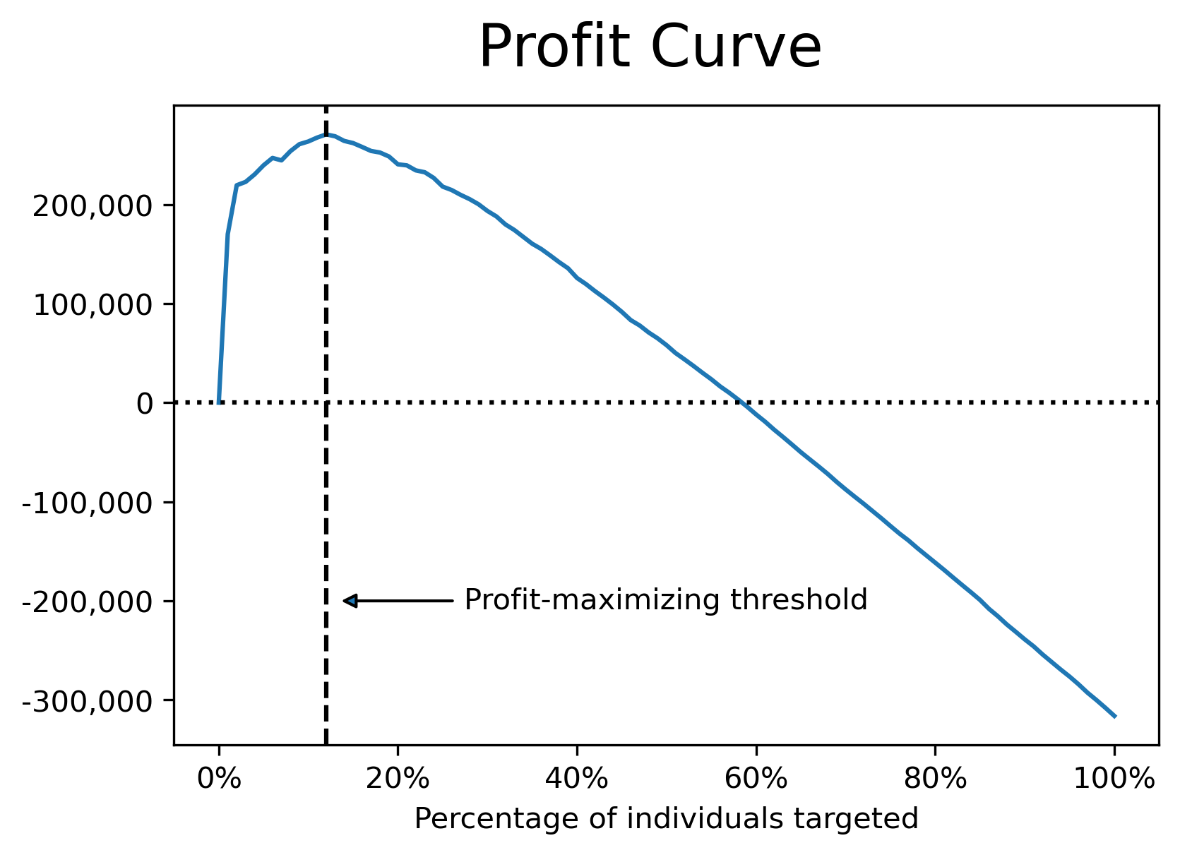
Figure 14: Cumulative profit when the top % of individuals with the largest causal scores are targeted.

In more intricate decision-making scenarios involving variable costs among individuals or complex constraints faced by the decision maker (McFowland III et al., 2021), the usefulness of EC and EO causal interpretations may be limited. However, future research could explore other causal interpretations beyond EE interpretation that could be valuable in more complex decision-making contexts. The concept of making predictions and subsequently utilizing them for optimization is commonly known as the predict-then-optimize paradigm in the operations literature. Researchers in this field acknowledge that minimizing prediction error without considering how the predictions will be utilized in downstream optimization problems is generally suboptimal (Elmachtoub and Grigas, 2022). Our framework builds upon this notion.

Causal scoring essentially entails estimating scores that can be endowed with causal interpretations that are useful for downstream optimization. Although we have focused on two interpretations that are pertinent to common (though relatively straightforward) decision-making processes, it is worth noting that our framework can accommodate other alternative interpretations that could prove useful in more complex decision-making scenarios.

7.2 Prevalence of Alternative Causal Interpretations

Causal interpretations of statistical estimates depend on assumptions about the underlying DGP that often cannot be tested with data. For example, the appropriate interpretation of findings in observational studies depends critically on the theoretical plausibility of non-testable assumptions such as ignorability. Consequently, the credibility of any causal interpretation hinges heavily on our theoretical comprehension of how the data were generated.

Full latent mediation and latent synchrony are two conditions concerning DGPs that are jointly sufficient for causal scores to have a valid EO interpretation. As with all fundamental assumptions that enable causal interpretations, these are non-testable assumptions. However, what is special about these assumptions is that they are always met when an EE interpretation is valid, as stated in Proposition 1. Therefore, they are less restrictive than any set of conditions that would allow us to interpret statistical estimates as causal effects.

Let us carefully analyze why this is the case. Another way to interpret the latent variable $L$ is as a signal that is captured by the causal scores and provides information about the causal effects. When we assert that an EE interpretation is valid, we are essentially claiming that the DGP is such that the signal captured by the scores perfectly matches the causal effects. In other words, we expect $\theta(X)=\mathbb{E}[L\mid X]=\beta(X)$.

Full latent mediation and latent synchrony describe DGPs where the captured signal does not exactly match the causal effects but at least indicates their direction. More specifically, full latent mediation implies that $X$ is predictive of causal scores and causal effects because of the same shared signal $L$, while latent synchrony implies that the signal behaves similarly in relation to causal scores and causal effects. Naturally, these conditions are weaker (and thus more likely to occur) than an exact match between causal effects and the signal captured by the causal scores.

This observation suggests that it may be possible to identify further instances of less stringent conditions under which causal methods can yield valuable insights. For instance, future research can explore the possibility of relaxing conditions such as the exclusion restriction in IVs or the parallel trends assumption in difference-in-differences analysis so that the statistical estimates still maintain a valid EO interpretation. The significance of causal scoring, a more comprehensive task than causal effect estimation, lies in its capacity to enhance our understanding of causal relationships across a broader spectrum of empirical scenarios.

However, determining how much broader the spectrum could be is an open question. How often are we in a situation where we can achieve a valid EO interpretation but not a valid EE interpretation? Answering this question empirically is highly challenging due to the non-testable nature of the conditions under consideration, but future research could explore this direction in settings where it is possible to collect unconfounded data. For example, Eckles and Bakshy, (2021) and Gordon et al., (2019) used data from controlled experiments to study the prevalence of valid EE interpretations in observational studies. In a similar fashion, we could use unconfounded data to evaluate and select causal scoring models based on their ability to rank or classify individuals according to their CATEs (Yadlowsky et al., 2021).

7.3 Methodological Developments

One of the primary motivations behind ML methods for causal effect estimation is the substantial improvement in performance that can be achieved when the method is designed to minimize the error in effect predictions instead of outcome predictions (Nie and Wager, 2021). The same idea motivates the design of ML methods for causal tasks beyond effect estimation.

Past studies have shown that learning to classify individuals into optimal actions can lead to better decisions than learning to accurately estimate effects (Lemmens and Gupta, 2020, Fernández-Loría et al., 2022, Zhang et al., 2012). Similarly, methods designed to identify the subpopulations most affected by a treatment can perform better at this task than methods designed for causal effect estimation (McFowland III et al., 2018). Therefore, a promising direction for future research is the design of ML methods for alternative causal interpretations.

For example, our theoretical results reveal that confounding bias can potentially improve the causal estimation for the purposes of effect ordering. This implies that ML methods aiming to completely eradicate confounding bias may not be ideal when our objective is an EO interpretation. Instead, we could benefit more from methods that selectively mitigate bias solely when it interferes with the intended causal interpretation of our estimates.

This observation is also critical for the development of methods that combine observational and experimental data (Peysakhovich and Lada, 2016, Rosenman et al., 2020, Kallus et al., 2018, Fernández-Loría and Provost, 2020) because depending on the DGP, the observational nature of the data could be desirable for improving effect ordering even if it is not useful for effect estimation.

More generally, a promising direction for future methodological developments is leveraging the causal interpretation we wish to give the causal scores as part of the causal estimation. This is closely related to recent developments in operations research, which aim to directly leverage the optimization problem structure—that is, its objective and constraints—for learning better predictive models (Elmachtoub and Grigas, 2022).

A key component in these developments is that the loss function used by the ML algorithm measures the decision error induced by the prediction. Therefore, prediction errors that do not induce decision errors are not penalized. In our context, the loss function could measure deviations from the causal interpretation we wish to attribute to the estimates, so that prediction errors that do not induce deviations from the target causal interpretation are not penalized.

Lastly, we anticipate that some of our findings can also be valuable in cases where the primary objective is effect estimation. For example, Leng and Dimmery, (2021) propose a method to calibrate and enhance the accuracy of causal effects, but the effectiveness of their approach depends on the uncorrected causal scores having the correct rank order (i.e., a valid EO interpretation). Similarly, Peysakhovich and Lada, (2016) propose the use of confounded effect estimates as additional features in experimental studies to improve the estimation of CATEs, which should help when the confounded estimates preserve the ranking of the CATE. In this paper, we provide a formalization of the conditions under which such methods may improve the accuracy of effect estimation for any type of causal scoring model.

APPENDIX

Appendix A Proof of Theorem 1

We want to show that, for any $\tau$, there exists a $\tilde{\tau}$ for which an EC interpretation is valid if an EO interpretation is valid. Without loss of generality, let $x_{i}$ be the feature values for the individual with the $i$-th largest CATE, so $\beta(x_{i})\geq\beta(x_{i+1})$. Therefore, given some $\tau$, there is a $k$ such that $\beta(x_{k})>\tau\geq\beta(x_{k+1})$. An EO interpretation implies that $\theta(x_{k})>\theta(x_{k+1})$, so we can set a $\tilde{\tau}$ such that $\theta(x_{k})>\tilde{\tau}\geq\theta(x_{k+1})$. We have that $\beta(x_{i})>\tau,\forall i\leq k$, and thus the EO interpretation implies that $\theta(x_{i})>\tilde{\tau},\forall i\leq k$. So, $\theta(x)>\tilde{\tau}$ if $\beta(x)>\tau$. Similarly, we have that $\beta(x_{i})\leq\tau,\forall i>k$, and thus the EO interpretation implies that $\theta(x_{i})\leq\tilde{\tau},\forall i>k$. So, $\theta(x)\leq\tilde{\tau}$ if $\beta(x)\leq\tau$. Therefore, an EC interpretation is valid. ∎

Appendix B Proof of Lemma 1

$$\beta(x) =\mathbb{E}[C\mid X=x]$$

$$=\mathbb{E}[\mathbb{E}[C\mid L,X=x]\mid X=x]$$

$$=\mathbb{E}[\mathbb{E}[C\mid L]\mid X=x]$$

$$=\mathbb{E}[\tilde{g}(L)\mid X=x]$$

$$=\mathbb{E}[\tilde{g}(\mu(x)+\epsilon)\mid X=x]$$

$$=\mathbb{E}[\tilde{g}(\mu(x)+\epsilon)]$$

$$=g(\mu(x)),$$

where we use the iterated expectations property on the second line, the third line follows by full latent mediation, the fourth line defines $\tilde{g}$ as the conditional expectation of $C$ given $L$, the fifth line follows by definition of $L$, the sixth line follows because $\epsilon$ is independent of $X$, and the seventh line defines $g$ as the expectation of $\tilde{g}(\mu(x)+\epsilon)$.

With an identical argument and using the definition of $\theta$ in Equation (4), we have:

$$\theta(x) =\mathbb{E}[S\mid X=x]$$

$$=h(\mu(x)).\qed$$

Appendix C Proof of Theorem 2

Full latent mediation implies that Lemma 1 is met, and therefore, $g_{\Delta}=\beta(x_{i})-\beta(x_{j})$ and $h_{\Delta}=\theta(x_{i})-\theta(x_{j})$. Full latent synchrony implies that $g_{\Delta}$ and $h_{\Delta}$ have the same sign. So, $\theta(x_{i})>\theta(x_{j})$ whenever $\beta(x_{i})>\beta(x_{j})$, and $\theta(x_{i})<\theta(x_{j})$ whenever $\beta(x_{i})<\beta(x_{j})$, which implies: $\theta(x_{i})>\theta(x_{j})\iff\beta(x_{i})>\beta(x_{j})$. ∎

Appendix D Proof of Proposition 1

If an EE interpretation holds for the CAS, then $\theta(x)=\beta(x)$ for all $x$. This implies that $\theta(x_{i})-\theta(x_{j})=\beta(x_{i})-\beta(x_{j})$. Thus, latent synchrony is met.

Full latent mediation is met by taking $L=\beta(X)=\theta(X)$. This implies that:

$$\mathbb{E}[C\mid L,X]=\mathbb{E}[C\mid\beta(X),X]=\mathbb{E}[C\mid X]=\beta(X)=L=\mathbb{E}[C\mid L]$$

and:

$$\mathbb{E}[S\mid L,X]=\mathbb{E}[S\mid\beta(X),X]=\mathbb{E}[S\mid X]=\theta(X)=\beta(X)=L=\mathbb{E}[S\mid L].$$

∎

Appendix E Proofs for Example 3

E.1 Derivation of baseline bias and CATT under Assumption 1.

First, the derivation of the baseline bias.

$$\mathbb{E}[Y^{0}\mid T=1,X]-\mathbb{E}[Y^{0}\mid T=0,X] =\mathbb{E}[\epsilon_{y}\mid\epsilon_{u}>-\psi(X),X]-\mathbb{E}[\epsilon_{y}\mid\epsilon_{u}\leq-\psi(X),X]$$

$$=\mathbb{E}[\mathbb{E}[\epsilon_{y}\mid\epsilon_{u}]\mid\epsilon_{u}>-\psi(X),X]-\mathbb{E}[\mathbb{E}[\epsilon_{y}\mid\epsilon_{u}]\mid\epsilon_{u}\leq-\psi(X),X]$$

$$=\alpha_{y}(\mathbb{E}[\epsilon_{u}\mid\epsilon_{u}>-\psi(X),X]-\mathbb{E}[\epsilon_{u}\mid\epsilon_{u}\leq-\psi(X),X])$$

$$=\alpha_{y}(\mathbb{E}[\epsilon_{u}\mid\epsilon_{u}>-\psi(X)]-\mathbb{E}[\epsilon_{u}\mid\epsilon_{u}\leq-\psi(X)])$$

The first line follows from the definitions of $Y^{0}$, $T$, and $U$, the second line from the law of total expectation, the third from Assumption 1, and the fourth line from the independence between $\epsilon_{u}$ and $X$.

Next, the derivation of the CATT:

$$\mathbb{E}[C\mid T=1,X] =\beta(X)+\mathbb{E}[\epsilon_{c}\mid\epsilon_{u}>-\psi(X),X]$$

$$=\beta(X)+\alpha_{c}\mathbb{E}[\epsilon_{u}\mid\epsilon_{u}>-\psi(X)].$$

The first line follows from the definitions of $C$, $T$, and $U$. The second line from the same arguments we used for the baseline bias. ∎

E.2 Derivative of the baseline bias under Assumption 2 and Assumption 3.

We know that the baseline bias is given by: $\alpha_{y}(\mathbb{E}[U\mid U>0,X]-\mathbb{E}[U\mid U\leq 0,X])$. We use Theorem 2 of Horrace, (2015), which gives an explicit expression for the derivative of the expectation of a truncated normal, which we can apply by Assumption 2. We obtain

$$\frac{d}{d\psi(X)}\alpha_{y}(\mathbb{E}[U\mid U>0,X]-\mathbb{E}[U\mid U\leq 0,X]) =\alpha_{y}\times(\mathrm{Var}(U\mid U>0)-\mathrm{Var}(-U\mid-U>0,X))$$

$$=\alpha_{y}\times(\mathrm{Var}(U\mid U>0)-\mathrm{Var}(U\mid U<0,X)).$$

With this expression at hand, we remark that $(\mathrm{Var}(U\mid U>0)-\mathrm{Var}(U\mid U<0,X))$ is equal to zero when $\psi(X)=0$, by symmetry of the Gaussian distribution. If we now prove that the difference in variances is an increasing function of $\psi(X)$, this implies the desired result. That is, the derivative of the bias has the same sign as $\psi(X)\times\alpha_{y}$. For this, we use Theorem 3 of Horrace, (2015) which implies:

$$\frac{d}{d\psi(X)}\mathrm{Var}(U\mid U\leq 0) =\frac{d}{d\psi(X)}\mathrm{Var}(-U\mid-U>0)$$

$$=-\frac{d}{d\psi(X)}\mathrm{Var}(U\mid U>0),\text{ and }$$

$$\frac{d}{d\psi(X)}\mathrm{Var}(U\mid U>0) >0.$$

The result follows by summing the two derivatives. ∎

E.3 Derivative of the CATT under Assumption 2 and Assumption 4.

As indicated previously, we can express the CATT by

$$\mathrm{CATT} =\beta(X)+\alpha_{c}\mathbb{E}[\epsilon_{u}\mid\epsilon_{u}>-\psi(X),X]$$

$$=\beta(X)+\alpha_{c}(\mathbb{E}[U\mid U>0,X]-\psi(X)).$$

With this at hand, and using the Theorem 2 of Horrace, (2015), to obtain the derivative with respect to $\beta(X)$ we do:

$$\frac{d}{d\psi(X)}\mathrm{CATT} =\frac{d\beta(X)}{d\psi(X)}+\alpha_{c}(\mathrm{Var}[U\mid U>0,X]-1).$$

The previous expression is greater than zero if and only if

$$\frac{d\beta(X)}{d\psi(X)}>\alpha_{c}(1-\mathrm{Var}[U\mid U>0,X]).$$

Since the variance of the truncated random variable is smaller than the variance of the random variable without truncation, and it is always positive, we have that $0<\mathrm{Var}[U\mid U>0,X]<1$. By Assumption 4, the effect on the treated increases with $\psi(X)$.

E.4 Confounded CAS has a valid EO interpretation.

The two previous sections have shown that the Assumptions 1-4 imply that each of the components of Equation (33) is increasing in $\psi(X)$. This implies that $(d\theta(X))/(d\psi(X))$ to be positive. Latent mediation for $C$ and $U$, and Lemma 1 implies that:

$$\mathbb{E}[C\mid L,X] =\mathbb{E}[C\mid L],$$

$$\mathbb{E}[U\mid L,X] =\mathbb{E}[U\mid L],$$

$$\beta(X) =g_{c}(\mu),\text{ and }$$

$$\psi(X) =g_{u}(\mu),$$

where $\mu=\mathbb{E}[L\mid X]$. Latent synchrony implies that for any $x_{i},x_{j}$ the sign of $g_{u}(\mu(x_{i}))-g_{u}(\mu(x_{j}))=\psi(x_{i})-\psi(x_{j})$ matches the sign of $g_{c}(\mu(x_{i}))-g_{c}(\mu(x_{j}))=\beta(x_{i})-\beta(x_{j})$.

To prove that the EO interpretation is valid we start with the “$\implies$”. Since $(d\theta(X))/(d\psi(X))>0$, for any $x_{i},x_{j}$ such that $\theta(x_{i})>\theta(x_{j})$ we know that $\psi(x_{i})>\psi(x_{j})$, by usual properties of derivatives. Latent synchrony implies that $\beta(x_{i})>\beta(x_{j})$.

Finally, to prove the “$\impliedby$”. Start with $\beta(x_{i})>\beta(x_{j})$, latent synchrony implies that $\psi(x_{i})>\psi(x_{j})$. Since $(d\theta(X))/(d\psi(X))>0$, we now have that $\theta(x_{i})>\theta(x_{j})$. ∎

Appendix F Proof of Theorem 3

By definition (Equation (40)):

$$\kappa=\frac{2}{n(n-1)}\sum_{i<j}\text{sgn}(\hat{\theta}(x_{i})-\hat{\theta}(x_{j}))$$

Taking the expectation results in:

$$\mathbb{E}[\kappa]= \frac{2}{n(n-1)}\sum_{i<j}\mathbb{E}[\text{sgn}(\hat{\theta}(x_{i})-\hat{\theta}(x_{j}))],$$

$$= \frac{2}{n(n-1)}\sum_{i<j}\mathbb{P}[\theta(x_{i})-\theta(x_{j})>0]-\mathbb{P}[\theta(x_{i})-\theta(x_{j})<0],$$

$$= \frac{2}{n(n-1)}\sum_{i<j}\left(2\mathbb{P}[\theta(x_{i})-\theta(x_{j})>0]-1\right),$$

$$= \left(\frac{4}{n(n-1)}\sum_{i<j}\mathbb{P}[\beta_{\Delta}+\alpha_{\Delta}+\xi_{\Delta}>0]\right)-1,$$

where on the last line, we denote: $\beta_{\Delta}=\beta(x_{i})-\beta(x_{j}),\alpha_{\Delta}=\alpha(x_{i})-\alpha(x_{j}),\xi_{\Delta}=\xi(x_{i})-\xi(x_{j})-\alpha_{\Delta}$. ∎

Appendix G Proof of Theorem 4

Full latent mediation implies that $g_{\Delta}=\beta(x_{i})-\beta(x_{j})$. Given that $x_{i}$ are the feature values for the individual with the $i$-th largest CATE, and $i>j$ in the definition of $\kappa$, then we have that $g_{\Delta}>0$. Equation (42) implies then that $h_{\Delta}>g_{\Delta}$. By definition of $\alpha_{\Delta}$, we have that:

$$\alpha_{\Delta} =\mathbb{E}[\xi\mid X=x_{i}]-\mathbb{E}[\xi\mid X=x_{j}]$$

$$=\mathbb{E}[\hat{\theta}(x_{i})]-\mathbb{E}[\hat{\theta}(x_{j})]-(\beta(x_{i})-\beta(x_{j}))$$

$$=\theta(x_{i})-\theta(x_{j})-(\beta(x_{i})-\beta(x_{j}))$$

$$=h_{\Delta}-g_{\Delta}>0$$

where the first line follows by definition of $\alpha$, the second line follows because of the definition of $\hat{\theta}$, the third line follows from the definition of $\theta$, and the last line follows from the definition of $g_{\Delta}$ and $h_{\Delta}$. ∎

Appendix H Proof of Corollary 1

If the algorithm used to learn $\hat{\theta}$ is a consistent estimator of $\theta$, then $\hat{\theta}(x)$ converges in probability to $\theta(x)$ as the amount of training data increases . This implies that $\hat{\theta}(x_{i})-\hat{\theta}(x_{j})$ converges in probability to $\theta(x_{i})-\theta(x_{j})$. Therefore, according to the definition of $\kappa$ in Equation (40), $\kappa$ converges in probability to:

$$\frac{2}{n(n-1)}\sum_{i<j}\text{sgn}(\theta(x_{i})-\theta(x_{j})).$$

Because the CAS has an EO interpretation, then the sign of $\theta(x_{i})-\theta(x_{j})$ is the same sign as $\beta(x_{i})-\beta(x_{j})$, which is positive. Then $\kappa$ converges in probability to

$$\frac{2}{n(n-1)}\sum_{i<j}1=1.$$

∎

Appendix I Other approaches for CATE estimation

This benchmark replicates the analysis in Section 6 with several other methods for CATE estimation. We used the implementation of the methods available in the CausalML package from Uber: https://github.com/uber/causalml. The methods we consider are:

1. Transformed outcome (TO): This is the same as the CATE-on-conversion model discussed in Section 6.

2. S-Learner (SL): See  Künzel et al., (2019) for details.

3. T-Learner (TL): See  Künzel et al., (2019) for details.

4. X-Learner (XL): See  Künzel et al., (2019) for details.

5. Causal Tree (CT): See Athey et al., (2016) for details.

6. Non-causal: This is the same as the conversion rate model discussed in Section 6.

Figure 15 shows that the results are qualitatively the same as in Section 6.3. None of the methods for causal effect estimation perform better than the “Non-causal” model at effect ordering or effect classification.

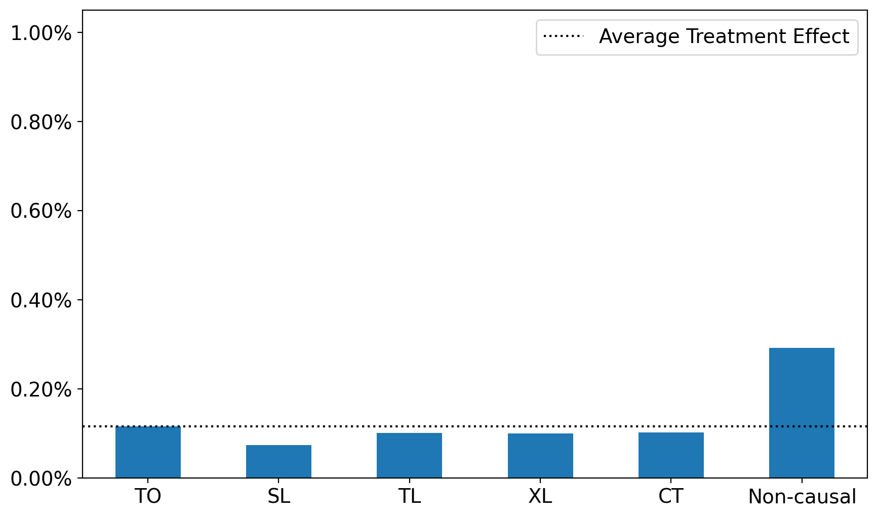
(a)

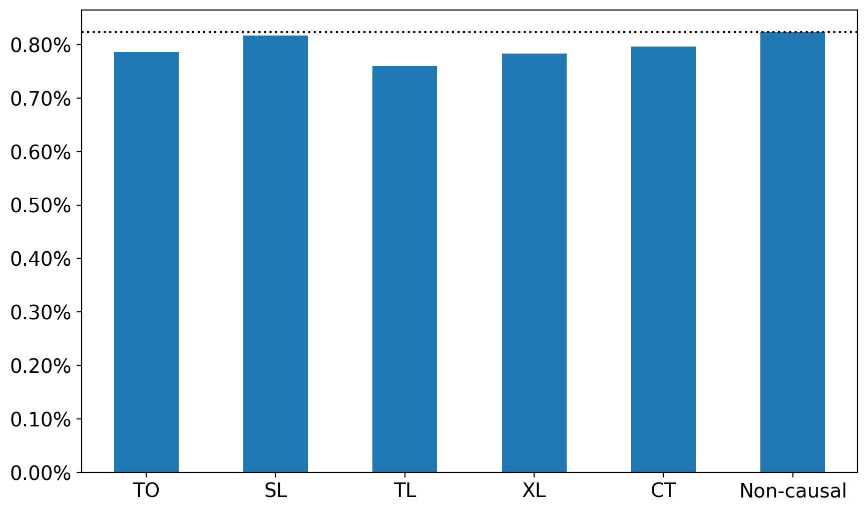
(b)

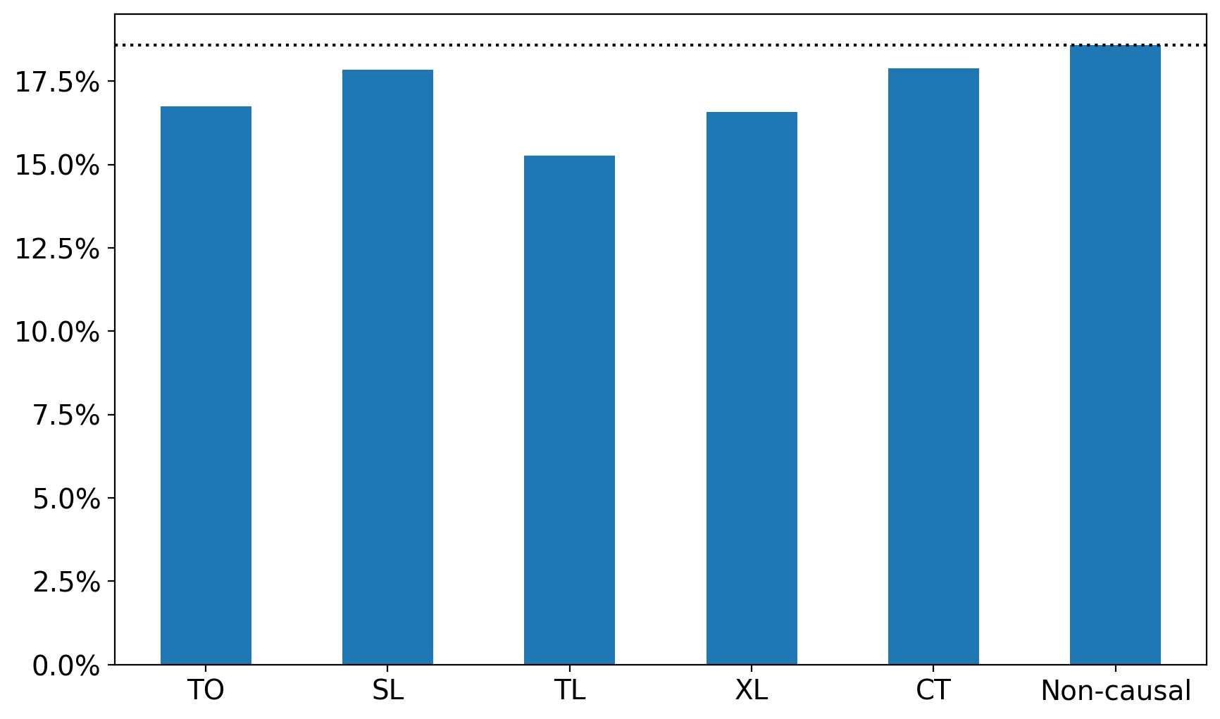
(c)

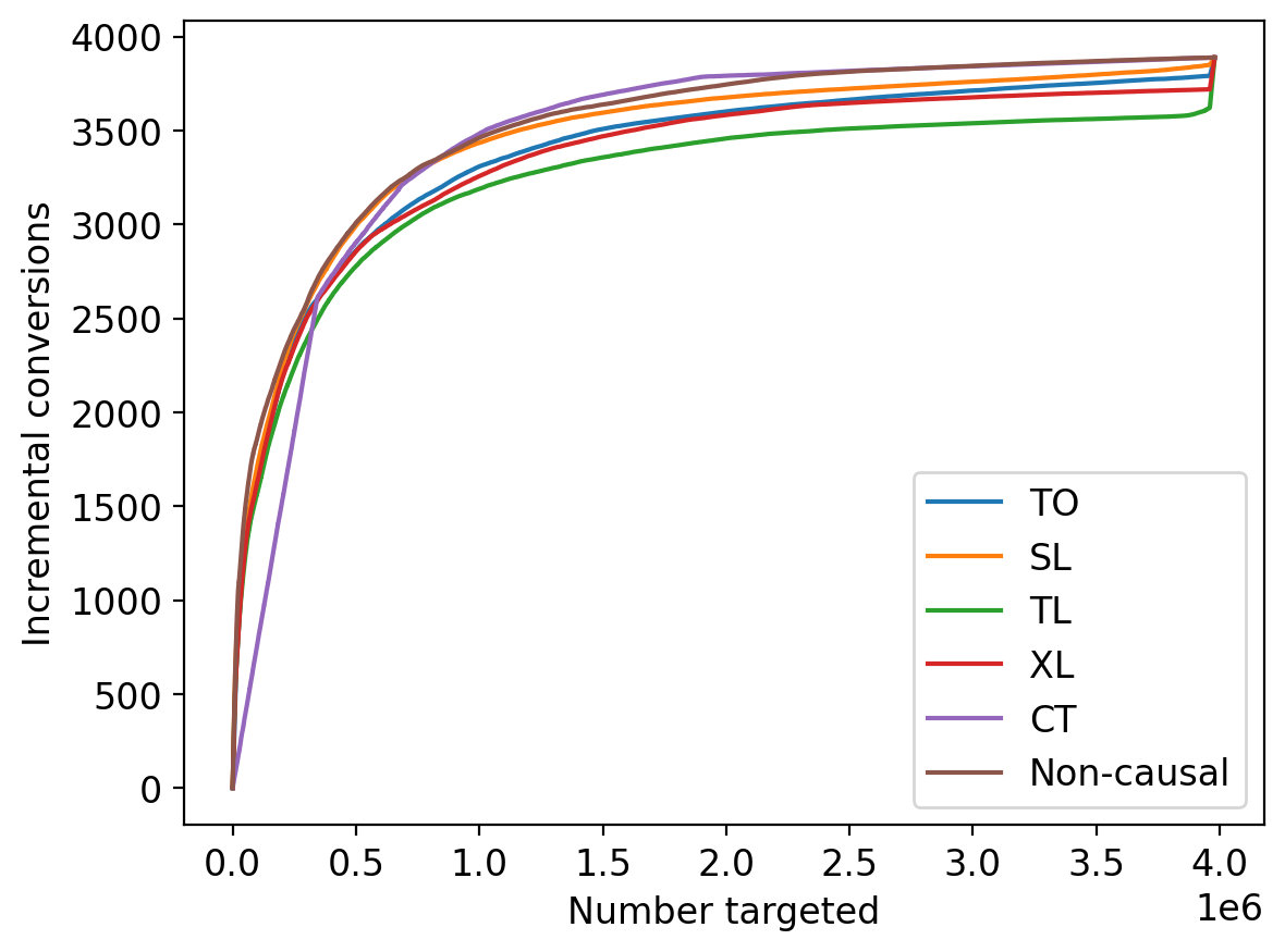
(d)

Figure 15: Comparison of causal scoring models. All models except for the “Non-causal” have a valid EE interpretation, but none perform better at effect ordering or effect classification.

References

- Angrist et al., (1996) Angrist, J., Imbens, G., and Rubin, D. (1996). Identification of causal effects using instrumental variables. Journal of the American statistical Association, 91(434):444–455.
- Ascarza et al., (2018) Ascarza, E., Neslin, S. A., Netzer, O., Anderson, Z., Fader, P. S., Gupta, S., Hardie, B. G., Lemmens, A., Libai, B., Neal, D., et al. (2018). In pursuit of enhanced customer retention management: Review, key issues, and future directions. Customer Needs and Solutions, 5(1):65–81.
- Athey et al., (2016) Athey, S., Chetty, R., Imbens, G., and Kang, H. (2016). Estimating treatment effects using multiple surrogates: The role of the surrogate score and the surrogate index. arXiv preprint arXiv:1603.09326.
- Athey and Imbens, (2016) Athey, S. and Imbens, G. (2016). Recursive partitioning for heterogeneous causal effects. Proceedings of the National Academy of Sciences, 113(27):7353–7360.
- Athey and Imbens, (2019) Athey, S. and Imbens, G. W. (2019). Machine learning methods that economists should know about. Annual Review of Economics, 11:685–725.
- Athey et al., (2023) Athey, S., Keleher, N., and Spiess, J. (2023). Machine learning who to nudge: causal vs predictive targeting in a field experiment on student financial aid renewal. arXiv preprint arXiv:2310.08672.
- Bhattacharya and Dupas, (2012) Bhattacharya, D. and Dupas, P. (2012). Inferring welfare maximizing treatment assignment under budget constraints. Journal of Econometrics, 167(1):168–196.
- Buyse et al., (2016) Buyse, M., Molenberghs, G., Paoletti, X., Oba, K., Alonso, A., Van der Elst, W., and Burzykowski, T. (2016). Statistical evaluation of surrogate endpoints with examples from cancer clinical trials. Biometrical Journal, 58(1):104–132.
- Dalessandro et al., (2015) Dalessandro, B., Hook, R., Perlich, C., and Provost, F. (2015). Evaluating and optimizing online advertising: Forget the click, but there are good proxies. Big data, 3(2):90–102.
- Diemert Eustache, Betlei Artem et al., (2018) Diemert Eustache, Betlei Artem, Renaudin, C., and Massih-Reza, A. (2018). A large scale benchmark for uplift modeling. In Proceedings of the AdKDD and TargetAd Workshop, KDD, London,United Kingdom, August, 20, 2018. ACM.
- Dorie et al., (2019) Dorie, V., Hill, J., Shalit, U., Scott, M., and Cervone, D. (2019). Automated versus do-it-yourself methods for causal inference. Statistical Science, 34(1):43–68.
- Eckles, (2022) Eckles, D. (2022). Commentary on “causal decision making and causal effect estimation are not the same… and why it matters”: On loss functions and bias–variance tradeoffs in causal estimation and decisions. INFORMS Journal on Data Science.
- Eckles and Bakshy, (2021) Eckles, D. and Bakshy, E. (2021). Bias and high-dimensional adjustment in observational studies of peer effects. Journal of the American Statistical Association, 116(534):507–517.
- Elmachtoub and Grigas, (2022) Elmachtoub, A. N. and Grigas, P. (2022). Smart “predict, then optimize”. Management Science, 68(1):9–26.