Dark photon vortex formation and dynamics

Abstract

We study the formation and evolution of vortices in $U(1)$ dark photon dark matter and dark photon clouds that arise through black hole superradiance. We show how the production of both longitudinal mode and transverse mode dark photon dark matter can lead to the formation of vortices. After vortex formation, the energy stored in the dark photon dark matter will be transformed into a large number of vortex strings, eradicating the coherent dark photon dark matter field. In the case where a dark photon magnetic field is produced, bundles of vortex strings are formed in a superheated phase transition, and evolve towards a configuration consisting of many string loops that are uncorrelated on large scales, analogous to a melting phase transition in condensed matter. In the process, they dissipate via dark photon and gravitational wave emission, offering a target for experimental searches. Vortex strings were also recently shown to form in dark photon superradiance clouds around black holes, and we discuss the dynamics and observational consequences of this phenomenon with phenomenologically motivated parameters. In that case, the string loops ejected from the superradiance cloud, apart from producing gravitational waves, are also quantised magnetic flux lines and can be looked for with magnetometers. We discuss the connection between the dynamics in these scenarios and similar vortex dynamics found in type II superconductors.

1 Introduction and summary

The dark photon Holdom:1985ag is a $U(1)$ vector boson which has been studied extensively as a candidate for new physics beyond the Standard Model. Motivated by string theory Arvanitaki:2009fg ; Goodsell:2009xc , the light vector field can play a significant role in dark matter direct detection Pospelov:2008jk ; Essig:2011nj , stellar An:2013yfc ; Hardy:2016kme , galactic Lasenby:2020rlf , and cosmological Jaeckel:2008fi ; Caputo:2020bdy dynamics. The bosonic nature of the dark photon allows it to be produced with very large amplitude in clouds around black holes that arise through superradiance Baryakhtar:2017ngi , and by inflationary perturbations as well as parametric resonance into dark photon dark matter Graham:2015rva ; Nelson:2011sf ; Agrawal:2018vin . Dark photon dark matter, in particular, is a prime target of a number of experiments Chaudhuri:2014dla ; PhysRevD.98.035006 ; PhysRevD.101.052008 ; PhysRevD.102.042001 ; PhysRevLett.125.171802 ; Chiles:2021gxk ; Cervantes:2022yzp .

At low energies and small amplitudes, the dark photon is described by the Proca action

$$\mathcal{S}=\int{\rm d}^{4}x\left(-\frac{1}{4}F^{\prime\mu\nu}F^{\prime}_{\mu\nu}-\frac{1}{2}m_{A^{\prime}}^{2}A^{\prime}_{\mu}A^{\prime\mu}\right),$$ (1)

which describes a massive vector field $A^{\prime\mu}$ with mass $m_{A^{\prime}}$ and field tensor $F^{\prime}_{\mu\nu}=\partial_{\mu}A^{\prime}_{\nu}-\partial_{\nu}A^{\prime}_{\mu}$. The Abelian Higgs model provides a UV completion of the Proca field above the scale $m_{A^{\prime}}$, and has the following action

$$\mathcal{S}=\int{\rm d}^{4}x\left[\frac{1}{2}\left|D^{\prime}_{\mu}\Phi\right|^{2}-\frac{1}{4}F^{\prime\mu\nu}F^{\prime}_{\mu\nu}-\frac{\lambda}{4}\left(|\Phi|^{2}-v^{2}\right)^{2}\right],$$ (2)

where $\Phi$ is complex scalar, $D^{\prime}_{\mu}\equiv\partial_{\mu}-ig_{D}A^{\prime}_{\mu}$ is the covariant derivative, and $g_{D}$ and $\lambda$ are coupling constants. We can write the complex scalar in terms of a phase and a radial displacement from its vacuum expectation value (VEV) $v$ as $\Phi=(v+\rho)\exp(i\Pi/v)$. The mass of the radial mode is $m_{\rho}=\sqrt{2}\lambda^{1/2}v$, while the dark photon mass is $m_{A^{\prime}}=g_{D}v$.

Dark photon dark matter searches are based on the limit where the quartic coupling $\lambda$ is taken to be infinite compared to the gauge coupling $g_{D}$, and the radial mode of the scalar $\Phi$ is taken to be infinitely heavy. Below the scale $\lambda^{1/2}v$, the radial mode can be integrated out, and the dynamics of the system is assumed to be described by the Stueckelberg action 2009esuf

$$\mathcal{S}=\int{\rm d}^{4}x\left[-\frac{1}{4}F^{\prime\mu\nu}F^{\prime}_{\mu\nu}-\frac{1}{2}\left(m_{A^{\prime}}A^{\prime}_{\mu}-\partial_{\mu}\Pi\right)\left(m_{A^{\prime}}A^{\prime\mu}-\partial^{\mu}\Pi\right)\right],$$ (3)

which reduces to the Proca action in the unitary gauge ($\Pi=0$). This action is sometimes assumed to be valid as long as the symmetry is not restored at strong field (see Lam:1971my ; tinkham2004introduction and Appendix B for more details):

$$g_{D}\rho_{A^{\prime}}^{1/2}\leq g_{D}B_{\rm c2}^{\prime}\equiv\lambda v^{2}$$ (4)

where $\rho_{A^{\prime}}=(E^{\prime 2}+B^{\prime 2})/2$ is the energy density due to the dark electric and magnetic fields.

This picture, however, is incomplete. Rather, there are vortex like solutions which are the lowest energy solution before the field strength reaches $B_{\rm c2}^{\prime}$ in eq. 4. In the limit of infinite $\lambda$, these vortex solutions are described by the Nambu-Goto action, integrated along the world sheet of the string vortex NambuGoto

$$\mathcal{S}=-\mu\int{\rm d}t{\rm d}l\sqrt{\gamma},$$ (5)

where the string tension $\mu$ is $\mathcal{O}(v^{2})$, with only a logarithmic dependence on the ratio between the string core size and the size of the region which contains the magnetic field [and hence up to $\log(\lambda/g_{D}^{2})$]. These vortex solutions are very similar to the vortices that form in type II superconductors, the well known Abrikosov vortices Abrikosov:1956sx (for more details about this analogy and the definition of the variables, see table 1). In all cases we consider, we find that the vortices form in background energy densities that are significantly smaller than $B_{\rm c2}^{\prime 2}=\lambda^{2}v^{4}/g_{D}^{2}$. In particular, they can form in a finite energy density in the limit $g_{D}\rightarrow 0$. The vortex solution is the energetically favorable solution in the background field as long as

$$\rho_{A^{\prime}}^{1/2}\gtrsim B_{\rm c1}^{\prime}\approx g_{D}v^{2}$$ (6)

when $\lambda\gg g_{D}^{2}$ Abrikosov:1956sx ; Nielsen:1973cs . Therefore, once formed, they will quickly dissipate energy stored in the dark photon dark matter or superradiance cloud and completely change the dynamics of the system as well as the phenomenological consequences. We will discuss in detail how these vortices form, how they evolve in the background dark electric and magnetic field, and the phenomenological consequences in the context of dark photon dark matter and a dark photon superradiance cloud.

In this work, we argue that vortex production occurs in all proposed dark photon dark matter production mechanisms Graham:2015rva ; Agrawal:2018vin ; Co:2018lka ; Dror:2018pdh ; Bastero-Gil:2018uel . During inflation, dark photon dark matter can be produced as longitudinal modes. If the Hubble parameter during inflation $H_{I}\gtrsim v$, regardless of if the $U(1)$ symmetry is restored or not, that is, independent of if $\lambda\rightarrow\infty$ ($m_{\rho}\gg H_{I}$), vortices will form. The evolution of these strings is qualitatively the same as ordinary cosmic gauged strings (see Appendix C.2 for some discussions about the differences), which after inflation approach a scaling solution.

Vortex production can also happen in the late Universe when energy is transferred from axions to the dark photon magnetic field Agrawal:2018vin ; Co:2018lka ; Dror:2018pdh ; Bastero-Gil:2018uel . In this case, the phase transition is a superheated phase transition when the magnetic field in the system reaches the superheating field

$$B_{\rm sh}^{\prime}\equiv\lambda^{1/2}v^{2}.$$ (7)

In the context of superconductors, at the superheating field, the transition between a phase with uniform magnetic field, to a phase with a large number of magnetic vortices, becomes a first order phase transition, though the magnetic field strength is still much smaller than $B_{\rm c2}^{\prime}$.

Though in the above we have borrowed terminology from the superconductor literature, the superheating field threshold, eq. 7, is parametrically the same as one would derive from equating the vector field energy density to the vacuum energy density of the Higgs $\rho_{A^{\prime}}\sim\lambda v^{4}$. Alternatively, one could consider the equation of motion for the radial mode, which is given by $\Box\rho=V_{\rm eff}^{\prime}(\rho)$ where

$$V_{\rm eff}=\frac{\lambda}{4}\left[(\rho+v)^{2}-v^{2}\right]^{2}+\frac{1}{2}g_{D}^{2}X(\rho+v)^{2}\mathrm{\ with\ }X=\left(A^{\prime}_{\mu}-\frac{1}{m_{A^{\prime}}}\partial_{\mu}\Pi\right)^{2}\ .$$ (8)

When $X\geq\lambda v^{2}/g_{D}^{2}$, the minimum of $V_{\rm eff}$ moves to $\Phi=0$ ($\rho=-v$) Fukuda:2019ewf . In the unitary gauge, which as noted above, is assumed when passing from the Abelian Higgs to the Proca action by taking $\lambda\rightarrow\infty$, $X=A^{\prime 2}$. Applying the condition on $X$ for the minimum of $V_{\rm eff}$ to move to the symmetry restoration point in this gauge with $\rho_{A^{\prime}}\sim m_{A^{\prime}}^{2}A^{\prime 2}$ again gives $\rho_{A^{\prime}}\sim\lambda v^{4}$. This simple argument ignores the spatial/temporal dependence of the vector field, but also suggests that we will expect some strong backreaction on the scalar field approaching this threshold.

In fact, when the superheating threshold is exceeded, a huge number of vortices, that is, cosmic strings, form all at once in the dark photon magnetic field, and most of the energy stored in the background magnetic field turns into energy of the cosmic strings until the electromagnetic field drops well below $B_{\rm sh}^{\prime}$. These cosmic strings radiate away their energy in the form of gravitational waves and boosted dark photons. At formation, the cosmic strings can have energy densities that are $\mathcal{O}(\lambda/g_{D}^{2})$ larger than the scaling energy density, and therefore, can contribute a burst of gravitational waves at the time of the superheated vortex forming phase transition.

Vortices can also form in a dark photon cloud that grows around a spinning black hole through the superradiant instability, as recently demonstrated in East:2022ppo . In black hole superradiance, a dark photon with Compton wavelength comparable to a spinning black hole will spontaneously form a gravitationally bound cloud that grows at the expense of the black hole’s rotational energy Pani:2012vp ; Endlich:2016jgc ; Baryakhtar:2017ngi ; East:2017mrj ; Cardoso:2018tly . In the Proca limit, where the dark photon only has gravitational interactions, the growth of the cloud will continue until the black hole is spun down below the superradiant regime brito_review ; East:2017ovw ; East:2018glu . In East:2022ppo , it was shown, using simulations with modestly large $\lambda/g_{D}^{2}\leq 50$, that approaching the superheating threshold, vortex strings are formed and subsequently accelerated by the dark electric field. They oscillate before being absorbed by the black hole, emitting a significant portion of the dark photon energy density from the cloud in a “stringy” bosenova event (analogous to the bosenova scenario proposed in axion superradiance Arvanitaki:2010sy ). Though in those cases, only a handful of strings formed, here we discuss how the dynamics may be different when $\lambda/g_{D}^{2}$ is very large, with up to $10^{38}$ strings forming at the same time in the superradiance cloud, and frequent string-string interactions leading to the exchange of energy, linear momentum, and angular momentum. In particular, this would allow for some strings to become gravitationally unbound from the black hole, with potentially observable consequences.

The paper is organized as follows. In section 2, we review the knowledge of these vortex solutions in the context of type II superconductor where they were first discovered. In sections 3 and 4, we discuss, analytically and numerically, how these vortices nucleate in dark photon dark matter from different production mechanisms. In section 5, we show the evolution of the vortices after its formation and the subsequent energy dissipation. In section 6, we discuss how vortices form and evolve in a dark photon superradiance cloud. We discuss the phenomenological consequence of these vortices both in the case of dark photon dark matter, as well as dark photon superradiance clouds in section 7. We make some final remarks in section 8 regarding how the dynamics studied in this paper can occur in other physical systems.

2 Dynamics of the Landau-Ginzburg model and the Abrikosov lattice

In this section, we review the dynamics of the Landau-Ginzburg model, the Abrikosov vortex and lattice solutions of type II superconductors, and the various phase transitions that occur as the strength of the magnetic field exceeds some threshold Abrikosov:1956sx ; tinkham2004introduction . We will use the language of the Abelian Higgs model, and point out several key differences between dark photon dark matter and type II superconductors.

2.1 Ground state

The Landau-Ginzburg model has a free energy that resembles that of equation 2, where the inverse of the mass of the dark photon $1/m_{A^{\prime}}$ is known as the London penetration depth $\delta$, and the inverse of the mass of the radial mode is $1/m_{\rho}$ is known as the coherence length $\xi$. The ratio between the two scales $\kappa\equiv\delta/\xi=\sqrt{\lambda/g_{D}^{2}}$ determines if the superconductor is type I or type II. For $\kappa>\frac{1}{\sqrt{2}}$, the superconductor is type II. The Stueckelberg limit corresponds to the case of $\kappa\rightarrow\infty$. In a type II superconductor, there are two critical fields. The critical field (the corresponding equation in the case of a dark photon $U(1)^{\prime}$ is shown in parentheses, also see table 1 in appendix D for a complete list of the terminology relevant to both systems)

$$H_{\rm c2}=\frac{\Phi_{0}}{2\pi\xi^{2}}\quad\left(B_{\rm c2}^{\prime}=\frac{\lambda v^{2}}{g_{D}}\right)$$ (9)

is the field strength at which superconductivity is completely lost, that is, the $U(1)$ symmetry is restored globally. Here $\Phi_{0}=\pi/e$ is the magnetic flux quantum. At this field strength, the mass of $\Phi$ (near $\Phi=0$)

$$m_{\Phi}^{2}=-\lambda v^{2}+gH$$ (10)

goes to zero and $\langle|\Phi|\rangle=v(1-gH/\lambda v^{2})^{1/2}\rightarrow 0$ becomes the global minimum, where $g=2e$ is the coupling of the Cooper pair to the photon. However, the field strength $H_{c2}$ is not the scale below which the superconducting state is the ground state. A state with a lattice of vortices (the Abrikosov lattice) has a lower free energy compared to the state where all the magnetic field lines are expelled (the Meissner effect) when the average magnetic field strength is larger than

$$H_{c1}\approx\frac{\Phi_{0}}{4\pi\delta^{2}}\log\kappa\quad\left(B_{\rm c1}^{\prime}=g_{D}v^{2}\log\frac{\lambda}{g_{D}^{2}}\right).$$ (11)

In the limit of large $\kappa$, this field strength is $\mathcal{O}(\log\kappa/\kappa^{2})$ smaller than $H_{c2}$.

At field strengths $H\gtrsim H_{c1}$, the ground state is comprised of a lattice of vortices. Each of the vortices has the following field profile in isolation in the $\kappa\rightarrow\infty$ limit

$$H(r)=\frac{\Phi_{0}}{2\pi\delta^{2}}K_{0}\left(\frac{r}{\delta}\right),$$ (12)

where $K_{0}$ is the zeroth-order Hankel function of imaginary argument. This function has the following asymptotic behaviour (see figure 1)

$$H(r)\approx\frac{\Phi_{0}}{2\pi\delta^{2}}\left(\frac{\pi\delta}{2r}\right)^{1/2}e^{-r/\delta},\quad r\gg\delta$$

$$H(r)\approx\frac{\Phi_{0}}{2\pi\delta^{2}}\left(\log\frac{\delta}{r}+0.12\right),\quad\xi\ll r\ll\delta.$$ (13)

The first equation above suggests that the size of the vortex is the magnetic penetration depth (the inverse of dark photon mass). The $\log(\delta/r)$ term in the second equation gives rise to a logarithmically divergent energy per unit length stored in the magnetic field in the limit where the string core size is taken to be zero, in agreement with the logarithmically large string tension in section 1.

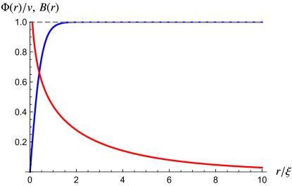
Figure 1: The field profile of an isolated vortex. The blue line is the profile of the radial mode $|\Phi(r)|$, which has a characteristic extent $\xi$, while the red line is the profile of the magnetic field, which has a characteristic extent $\delta$. Here we take $\delta/\xi=10$.

At field strengths of $H_{c1}\ll H\ll H_{c2}$, the ground state is known as the Abrikosov lattice, where the vortices line up in a 2D lattice with lattice spacing

$$a_{L}=c_{L}\left(\Phi_{0}/H\right)^{1/2}\ll\delta,$$ (14)

where $c_{L}$ is an $\mathcal{O}(1)$ number which depends on the structure of the lattice of the vortices (see figure 2). The force between two vortex lines is repulsive, due to the overlap of the magnetic field when $a_{L}\ll\delta$ ($\kappa>1/\sqrt{2}$, to be exact). However, when $a_{L}\ll\delta$, a large number of vortices overlap with each other, and the system exhibits complicated vortex matter dynamics ( see RevModPhys.90.015009 ).

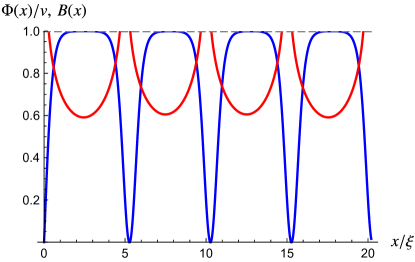
Figure 2: The field profile of a vortex lattice in a 1D slice. The blue line is the profile of the radial mode $|\Phi(x)|$, which has a characteristic extent of $\xi$, while the red line is the profile of the magnetic field, whose periodicity is the lattice spacing $a_{L}$. Here we take $\delta/\xi=10$ and $a_{L}/\xi=5$.

2.2 Superheating

The phase transition between the vortex lattice phase and the Meissner phase is a first order phase transition when $H\gtrsim H_{c1}$. This is to be expected since the two phases have very different spacetime symmetries, as well as topologies. In particular, when $\kappa\rightarrow\infty$, the vortex solution has a profile with typical size $\xi$, while the profile for the vector potential has a typical size $\delta$. The system can remain in the Meissner phase until $H=H_{\rm sh}$, the superheating field, when this phase transition becomes a second order phase transition Galaiko1966FormationOV ; osti_4551407 ; liarte2016ginzburg ; PhysRev.170.475 ; PhysRevB.65.144529 . The superheating field is

$$H_{\rm sh}=C_{\rm sh}\Phi_{0}/\delta\xi\quad\left(B_{\rm sh}^{\prime}=\lambda^{1/2}v^{2}\right),$$ (15)

where $C_{\rm sh}$ is an $\mathcal{O}(1)$ coefficient that depends on the geometry of the system. At the superheating field, a linear combination of the vector potential and the order parameter becomes tachyonic, and the phase transition becomes second order. A qualitative picture of this instability is shown in figure 3. As the magnetic field approaches $H_{\rm sh}$, a localized perturbation of magnetic field causes the $|\Phi|$ field to also develop a localized profile (see equation 10). This localized dip in $\langle|\Phi|\rangle$ causes the magnetic field to further cluster (similarly to the Meissner effect), leading to a runaway effect, and a vortex is formed despite the initial background magnetic field being much smaller than the critical field $H_{c2}$. In this instability, the clustering magnetic field only needs to overcome the mildly growing gradient energy in the fields, leading to the formation of a defect in a field that seems decoupled in the $\lambda/g^{2}\rightarrow\infty$ limit.

Recent studies PhysRevB.83.094505 have identified the most tachyonic mode as a vortex like excitation with a typical momentum $k_{c}\simeq\kappa^{3/4}/\delta$, instead of either $1/\delta$ or $1/\xi$. Compared to the lattice spacing $a_{L}$ at the superheating field computed from equation 14,

$$k_{c}a_{L}\sim\kappa^{1/4}.$$ (16)

This further highlights that the vortices nucleated at the superheating field have profiles and structures that are very far from the eventual equilibrium state. As we will see, this can have distinct phenomenological consequences for dark photon dark matter.

At field strengths below the superheating field, the phase transition is first order. The barrier in free energy between the two phases was first studied in Galaiko1966FormationOV , where it was found that the barrier in free energy is $\Delta F\sim\Phi_{0}^{2}\xi(\log\kappa)^{2}/\delta^{2}\sim v(\log\kappa)^{2}/\lambda^{1/2}$ for a thermal phase transition. The vacuum phase transition, which is more important for our understanding of the stability of dark photon dark matter in the late universe, has not, as far as the authors know, been well understood analytically due to the very limited symmetry of the bounce action.

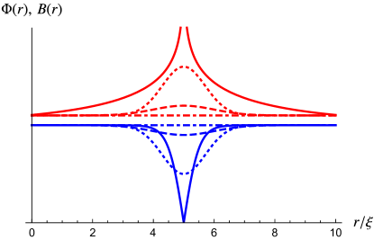
Figure 3: The field profile evolution when the field strength approaches the superheating field. The magnetic field $B$ (red lines) and the scalar field magnitude $|\Phi|$ (blue lines) are both constant in the beginning (dot-dashed). A small perturbation in the magnetic field (dashed) leads to a localized $\Phi$ profile. This causes magnetic field to further cluster in the region where $\langle\Phi\rangle$ is small (dotted) and the scalar profile to further develop a dip. The magnetic field grows logarithmically to infinity in this localized region, eventually pushing $\Phi$ to zero, creating a vortex. The solid lines show the profiles of a localized vortex as reference.

2.3 Melting phase transition

Following a superheated phase transition, vortex lattices in type II superconductors exhibit a melting phase transition for large ${\lambda/g_{D}^{2}}$. The melting phase transition in the context of a vortex lattice is the formation of many small vortex loops such that the vortex-vortex correlation functions decays as the vortex separation grows, and as a result, the translational symmetry broken by the background magnetic field and the vortex lattice is restored zeldov1995thermodynamic ; james2021emergence ; liu1991kinetics ; PhysRevB.8.3423 .

The superheated phase transition occurs between two states that have very different free energy density, which suggests that the superheated phase transition produces a network of vortices that is very far from the ground state configuration in the same background magnetic field. After the phase transition, a network of vortex lines with total length that is $\mathcal{O}(\kappa)$ times larger than the length of vortex lines of the ground state (in the same background magnetic field) can be formed. This network of vortices, through vortex reconnections, produces small loops of vortices with random locations and orientations. As the melting phase transition eventually completes, the mostly straight lines that align with the external magnetic field have lengths that are $\mathcal{O}(1/\kappa)$ of the total length of vortex lines in the system. The small loops therefore dominate the vortex-vortex correlation functions, and an approximate translational symmetry is restored in this vortex fluid despite the background magnetic field.

3 Vortex formation in dark photon dark matter

The existence of these vortex solutions and vortex formation mechanisms raises concerns about whether the light $U(1)^{\prime}$ dark photon has a viable production mechanism to be a dark matter candidate. The best-motivated production mechanism for light dark photon is inflationary production Graham:2015rva , which produces a dark photon longitudinal mode through inflationary perturbations. Recently, there have been proposals for a new tachyonic particle production mechanism Agrawal:2018vin , which predominantly generates magnetic field that later redshifts to be cold dark matter. In this section, we show how vortices form in both cases.

3.1 Vortex Formation: Longitudinal mode

In the case of inflationary production, vortex formation happens as long as the inflationary scale $H_{I}>v$. In the limit of infinite $\lambda$, the effective action is a combination of the Proca action plus the Nambu-Goto string action. The production rate of Nambu-Goto string during inflation PhysRevD.44.340

$$\Gamma\sim\exp[-4\pi\mu/H_{I}^{2}],$$ (17)

where $\mu\sim\pi v^{2}\log(\min[\lambda/g_{D}^{2},m_{\rho}/H_{I}])$ is the string tension. The logarithm comes from the logarithmically divergent string tension, where the UV scale is the radius of the string core (scalar profile), while the IR scale is the larger of the mass of the dark photon, or the Hubble scale during inflation. For $v\lesssim H_{I}$, there will be $\mathcal{O}(1)$ strings produced in each Hubble volume per Hubble time. Even if $v\gtrsim H_{I}$, as we elaborate in appendix C.2, a string network that eventually approaches a scaling solution can still be produced.

In the case of longitudinal mode production, the formation does not suffer from a suppression due to superheating because the longitudinal mode fluctuation itself generates the vortex. The $\Pi$ field has a $2\pi$-periodicity of $\Pi/v\rightarrow\Pi/v+2\pi$. The longitudinal mode $A_{L}$ inherits this periodicity. A large amplitude of $\Pi$ and $A_{L}$ means that the field winds around many times, which is equivalent to producing a large number of vortices. In order to not produce these vortices, we need the scalar VEV $v>H_{I}$. Given that the dark matter density is Graham:2015rva

$$\Omega_{\rm A^{\prime}}=\Omega_{\rm DM}\times\sqrt{\frac{m_{A^{\prime}}}{6\times 10^{-6}\,{\rm eV}}}\left(\frac{H_{I}}{10^{14}\,{\rm GeV}}\right)^{2},$$ (18)

we have

$$g_{D}=\frac{m_{A^{\prime}}}{v}\leq\frac{m_{A^{\prime}}}{H_{I}}=2\times 10^{-22}\left(\frac{m_{A^{\prime}}}{\rm eV}\right)^{5/4}.$$ (19)

For a kinetic mixing with the standard model photon of $\epsilon\sim g_{D}e/(16\pi^{2})$ Holdom:1985ag , this corresponds to $\epsilon<10^{-24}$, about ten orders of magnitude beyond current experimental capabilities.

One possible way to evade this limit is to introduce a charge hierarchy of $10^{10}$ between the particle that runs in the loop to generate the kinetic mixing and the Higgs Gherghetta:2019coi . These models are constructed mainly to explain the smallness of the kinetic mixing parameter as compared to the gauge coupling $g_{D}$. To evade our constraints, one needs to run the clockwork mechanism backwards. We makes some additional remark on this possibility in appendix C.1. A second possible way out is to introduce a large non-minimal coupling to gravity that suppresses string production. However, this does not solve the problem of producing enough dark photon dark matter; we elaborate on this possibility in appendix C.2.

The quartic $\lambda\rightarrow\infty$ limit is the simplest way to achieve a Stueckelberg mass for a $U(1)^{\prime}$ dark photon, which works perfectly in scenarios where collective effects are inaccessible. A few other UV completions have been studied to generate a small dark photon mass and kinetic mixing Goodsell:2009xc , motivated by string theory. In these cases, the lightness of the radial mode (or other charged particles) is not related to the smallness of the dark photon mass, the dark gauge coupling, and the kinetic mixing in the same way as the cases studied in this paper. However, there generically exist new states below the Hubble scale in eq. 18, whose dynamics can significantly disrupt the dark photons, either by vortex formation, in the cases where there is a charged scalar, or as in the scenarios studied in Arvanitaki:2021qlj , if there are only charged fermions. We will not comment further on these scenarios since there are no concrete models, as far as the authors know, where a small dark photon Stueckelberg mass is generated in a theory where the string scale is above the Hubble scale during inflation implied in equation 18. The weak gravity conjecture Arkani-Hamed:2006emk ; Reece:2018zvv places some doubt on whether such a scenario can be reliably constructed in string theory to produce a light dark photon as dark matter. Combining the weak gravity conjecture $g_{D}\gtrsim m_{\rho}/m_{\rm Pl}\gtrsim H_{I}/m_{\rm Pl}$ and $g_{D}\leq m_{A^{\prime}}/H_{I}$ with eq. 18 suggests that $m_{A^{\prime}}\gtrsim 50\,{\rm GeV}$.

3.2 Vortex Formation: Transverse mode

In the background of a transverse dark photon, the dynamics of vortex formation is similar to vortex formation in a superconductor. The presence of the magnetic field (flux) is essential. However, the production of vortices is not significantly hindered by the presence of a similar-sized or larger (on average) electric field, as long as there is no Lorentz transformation that can remove the magnetic field everywhere, and, in fact, the strength of the electric field can aid in crossing the superheating threshold. This is demonstrated by the case of the superradiant dark photon cloud, where the vector field is electrically dominated, and vortex formation happens when $-F^{\prime 2}$ approaches $\sim B^{\prime 2}_{\rm sh}$. We will describe this in more detail in section 6.

Magnetic mode

In a background magnetic field, vortices should form when the background magnetic field exceeds a similar superheating field of $B^{\prime}_{\rm sh}$, just like in the case of a superconductor. However, there are some key differences between vortex formation in superconductors and in dark photon dark matter. The most important difference is that in the case of superconductor, the phase transition happens between the Meissner phase and the Abrikosov lattice phase, where there is originally zero magnetic field inside the bulk of the superconductor (the Higgs phase). All vortices enter from the edge of the superconductor. However, in the case of dark photon dark matter, there is already an oscillating electric field and magnetic field inside the bulk where the dark photon is in the Higgs phase. The second main difference is that a superconductor always has an edge where vortex lines can end on, since beyond the edge of the superconductor, the photon is massless. However, in the case of dark photon dark matter, the whole Universe is in the Higgs phase and the vortices have to form as string loops. Lastly, in both dark photon dark matter and a dark photon superradiance cloud, there are usually electric fields of similar size or larger in the same system, which can affect vortex formation. Due to the above-mentioned differences, in the next section we perform several numerical studies of vortex formation in dark photon dark matter.

Electric mode

It is unclear what the production mechanism for a transverse mode of a dark photon that is purely electric field would be, since this would mean such modes can be produced with zero momentum dependence. On the other hand, if there were some unknown mechanism for producing transverse mode dark photon dark matter at the time of CMB, then the dark photon dark matter would be predominantly electric field mode due to redshifting.

In a purely curl-free electric field background, vortex formation does not happen. As the field strength of the electric field reaches $g_{D}E^{\prime}\gtrsim m_{A^{\prime}}m_{\rho}$ (or equivalently, $E^{\prime}\gtrsim B^{\prime}_{\rm sh}$), the heavier scalar field and the lighter dark photon field oscillators become strongly coupled and energy can be transferred between the dark photon and the radial mode. When the electric field is small, the energy that oscillates into the radial mode grows as $E^{\prime 4}$ when $E^{\prime 2}<\lambda v^{4}$. As the dark photon field continues to grow, the system becomes non-linear. However, since both energies redshift like matter, it is unclear if these oscillations significantly change the dark photon density after $E^{\prime 2}$ eventually drops below $\lambda v^{4}$.

4 Vortex formation in magnetic dark photon production

In this section, we study numerically how vortices form in dark photon dark matter in production mechanisms where the dark photon is produced initially as dark magnetic field. As shown in some recent studies Agrawal:2018vin ; Co:2018lka ; Dror:2018pdh ; Bastero-Gil:2018uel , dark photon dark matter can also be produced in the late Universe by invoking a coupling between the dark photon and rolling axion field $a$ of the form

$$\mathcal{S}=\int{\rm d}^{4}x\left(\ldots+\frac{a}{f}F^{\prime}_{\mu\nu}\tilde{F}^{\prime\mu\nu}\right)\ ,$$ (20)

where $f$ is the axion decay constant. In the background of a time dependent axion field $\dot{a}/f\neq 0$, the dark photon dispersion relation is

$$\omega^{2}=(|\boldsymbol{\mathbf{k}}|\pm\dot{a}/2f)^{2}-(\dot{a}/2f)^{2}+m_{A^{\prime}}^{2}-H^{2}/4.$$ (21)

Thus, modes with wavenumbers in the range $k\in[k_{-},k_{+}]$ where

$$k_{\pm}=\dot{a}/2f\pm\sqrt{(\dot{a}/2f)^{2}-m_{A^{\prime}}^{2}+H^{2}/4}$$ (22)

can grow exponentially in time, with the fastest growing mode having wavenumber $k_{p}=(k_{+}+k_{-})/2$. This instability can efficiently transfer energy from the axion field $a$ to the dark photon electric and magnetic fields if $\dot{a}/2f\geq m_{A^{\prime}},H$. The exact fraction of energy in the electric and magnetic field at any time depends on the relative size of the parameter $\dot{a}/2f$, $m_{A^{\prime}}$ and $H$, and the shape of the axion potential. Nevertheless, at the time when the tachyonic instability stops and the $A^{\prime}$ density is at its peak, $\omega\sim k\geq m_{A^{\prime}}$ and a significant portion of the energy is stored in the magnetic field. A large dark magnetic field (in particular, $\boldsymbol{\mathbf{E}}^{\prime}\cdot\boldsymbol{\mathbf{B}}^{\prime}$) can backreact on the rolling axion field. The leading effect of this is to slow down the rolling axion (decreasing $\dot{a}$), which stops dark photon production. Throughout the paper, we restrict to regions of the parameter space where the backreaction of the gauge field on the rolling axion field is small.

As suggested in section 2, vortex formation can occur if the magnetic field generated by the tachyonic instability grows sufficiently large. We use numerical simulations to explore the formation and subsequent dynamics of the vortices. Since this is our primary interest, we will ignore the cosmological evolution and backreaction of the axion field, and numerically evolve the Abelian-Higgs equations in the Lorenz gauge ($\partial_{\mu}A^{\prime\mu}=0$) with a source term due to a homogeneous rolling axion background. The vortex formation dynamics is independent of the reshifting of the gauge fields, while the subsequent evolution of the strings post-vortex formation will depend on cosmic expansion. Given the large amount of energy that needs to be dissipated to reach close to a scaling solution for moderate $\lambda/g_{D}^{2}$, it is likely very challenging to track the full dynamics in an expanding universe based on what has been achieved in the literature for similar and slightly simpler systems Buschmann:2021sdq . See section A for details on the evolution equations and numerical methods.

4.1 Two-dimensional results

We begin with results assuming a translational symmetry in one direction. This makes tackling the large $\lambda/g_{D}^{2}$ regime more computationally tractable, and more straightforwardly connects to the Abrikosov lattice picture of section 2. However, we also perform fully 3D simulations, to highlight the similarities and differences from the 2D case, which we discuss in the next section.

As the vector field grows exponentially due to the tachyonic instability, the scalar field becomes increasingly displaced from its VEV towards lower magnitudes in the regions of high dark photon field. We illustrate a representative case with $\lambda/g_{D}^{2}=100$ in figure 4. There, the maximum of $1-|\Phi|/v$ can be seen to track the maximum of $F^{\prime 2}/(4\lambda v^{4})$. This agrees with the shift in the minimum of $V_{\rm eff}$ in eq. 8 since $F^{\prime 2}\approx m_{A^{\prime}}^{2}X$ in the linear instability phase. This persists until $\Phi=0$ somewhere in the domain, which marks the onset of vortex formation. Shortly after vortex formation, we switch off the axion source term (see section A for details), which halts the growth of the vector field. In the exponential growth phase, the vector field is everywhere magnetically dominated, $F^{\prime 2}>0$. However, post-vortex formation, the vector field decays as energy is transferred from the vector to scalar sectors. One can also see oscillations occurring at a frequency of $\sim 2m_{A^{\prime}}$ between regions of strong electric dominance (i.e. $F^{\prime 2}$ negative and large in magnitude) and magnetic dominance. We will describe this in more detail below.

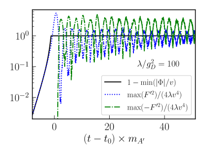
Figure 4: Maximum and minimum field values as a function of time. We show the displacement from the VEV of the minimum scalar field magnitude (solid black line), which tracks the maximum of the field tensor contracted with itself $F^{\prime 2}$ (dotted blue line) closely during the linear instability phase. We also show the maximum values of $-F^{\prime 2}$ (dashed-dotted green line) when this quantity is positive. Here $F^{\prime 2}\equiv F^{\prime\mu\nu}F^{\prime}_{\mu\nu}=2(B^{\prime 2}-E^{\prime 2})$, so $F^{\prime 2}>0$ corresponds to magnetic dominance, and $F^{\prime 2}<0$ corresponds to electric dominance.

The vortices are characterized by places where the magnitude of $\Phi$ goes to zero, and the complex phase goes through some non-zero multiple of $2\pi$ when encircling the point. This can be seen in figure 5, where the scalar field configuration is illustrated. As $\lambda/g_{D}^{2}$ is increased, the main difference is that the characteristic size of the vortices decreases, and their density increases. This is illustrated in figure 6, where we compare a case with $\lambda/g_{D}^{2}=100$ to $\lambda/g_{D}^{2}=400$.

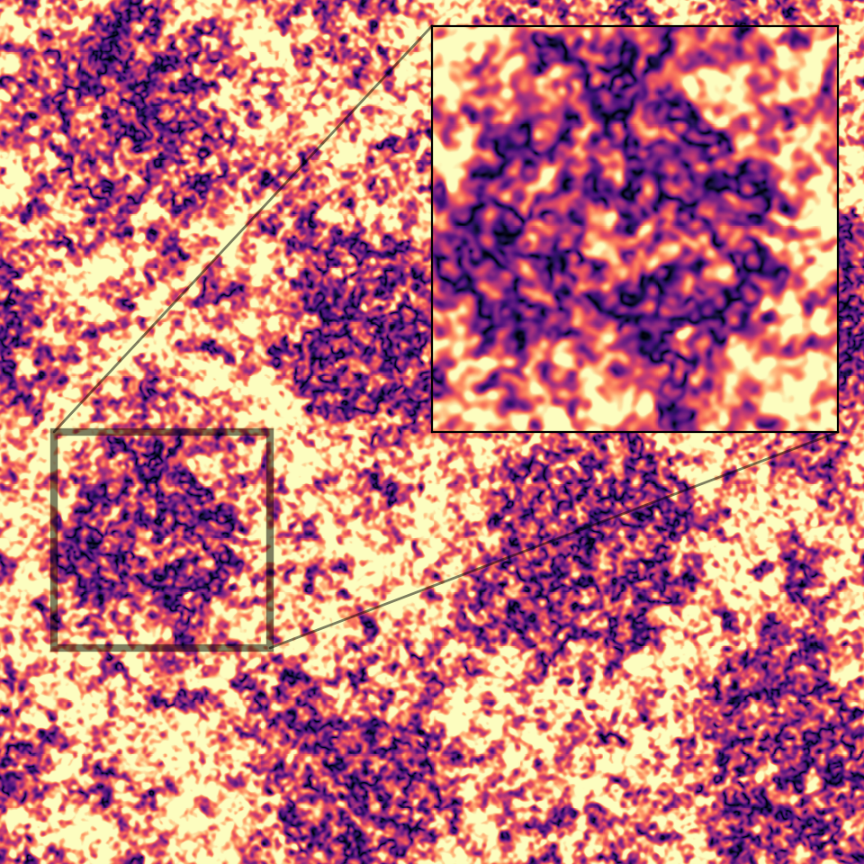
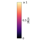
Figure 5: Snapshot at late times of the complex scalar $\Phi$ from the same case with $\lambda/g_{D}^{2}=100$ shown in figure 4. The left panel shows the magnitude of $\Phi$, while the right panel shows the complex phase. In both panels, the inset at the top right shows a zoom-in of a region where a number of vortices have formed. The length of the domain is twice the wavelength of the dominant mode of the axion instability, the latter of which is approximately equal to the Compton wavelength of the dark photon ($L=4\pi/k_{p}$ where $k_{p}\approx 1.055m_{A^{\prime}}$). A translational symmetry is assumed in the out-of-page direction.

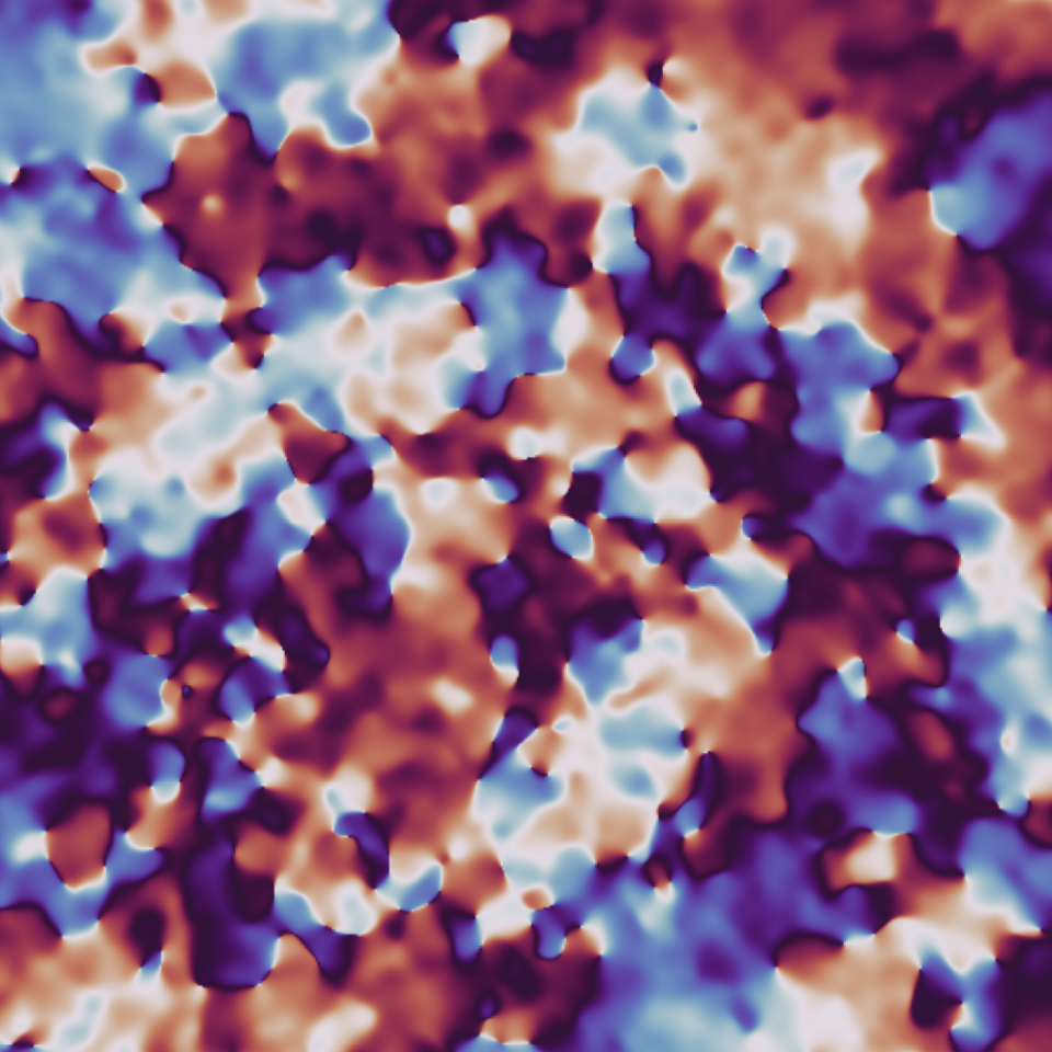
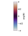
Figure 6: Snapshot of the complex phase of $\Phi$ for $\lambda/g_{D}^{2}=100$ (left) and $\lambda/g_{D}^{2}=400$ (right) at approximately the same time ($\approx 30/m_{A^{\prime}}$ after vortices form) over a portion of the domain of length $\approx\pi/m_{A^{\prime}}$. This illustrates the increasing density of vortices as $\lambda/g_{D}^{2}$ is increased.

After the vortices form, the dark photon field does work on them, transferring energy from the scalar to the vector sector. We discuss this dynamics analytically in more detail in section 5. To quantify this, we compute the energy $E$, or equivalently, average energy density $\langle\rho\rangle$, for the vector field

$$E_{A^{\prime}}=\langle\rho_{A^{\prime}}\rangle L^{3}=\frac{1}{2}\int\left(E^{\prime 2}+B^{\prime 2}\right)dV\ ,$$ (23)

and the scalar field

$$E_{\Phi}=\langle\rho_{\Phi}\rangle L^{3}=\int\left[\frac{1}{2}|D_{t}\Phi|^{2}+\frac{1}{2}|D_{i}\Phi|^{2}+\frac{\lambda}{4}\left(|\Phi|^{2}-v^{2}\right)^{2}\right]dV\ ,$$ (24)

where we have included the interaction energy (i.e. terms involving both $A^{\prime}$ and $\Phi$) in the latter. We show these quantities as a function of time in the left panel of figure 7 for three different cases where we vary the time at which the axion instability shuts off, and hence the magnitude to which the vector field grows. When no vortices form (black curves in left panel of figure 7), there is little energy transfer between the vector and scalar sectors, and the scalar energy remains subdominant. In this case, the presence of the radial mode and the energy transfer between the two components do not significantly affect the evolution of the energy density. Such is also the case in a background electric field. When vortices do form, the vector field can do work on them, with energy moving from the vector into the scalar sector until the latter becomes dominant (see section 5.1 for further discussion of this). In this regime, this is largely independent of the exact value of $\lambda/g_{D}^{2}$, as is demonstrated in the right panel of figure 7, where we compare several cases with $\lambda/g_{D}^{2}=100$, 200, and 400.

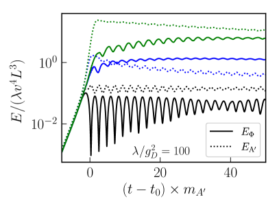
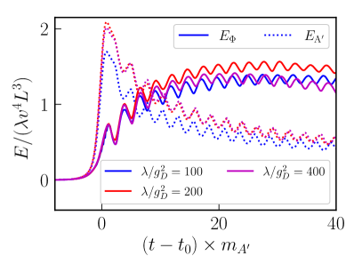
Figure 7: Energy in the scalar field (including interaction energy with the vector; solid lines) and energy in the vector field (not including interaction energy; dashed lines) as a function of time. Left Panel: We show three different cases with $\lambda/g_{D}^{2}=100$ where the time $t_{0}$ when the axion instability is shut off increases by increments of $\approx 1.2/m_{A^{\prime}}$ going from black, to blue, to green. In the case when the axion instability is shut off the earliest (black lines), no vortices form, while in the other two cases, they do. For the x-axis, time is scaled to the value of $t_{0}$ for the intermediate case (blue curves). Right Panel: We compare three different cases with $\lambda/g_{D}=100$, 200, and 400, and with $t_{0}$ chosen to give approximately the same value of $E_{\Phi}/\lambda$ at the time when the instability is shut off. The blue curves ($\lambda/g_{D}^{2}=100$) are the same case as in the intermediate case in the left panel.

The vector field configuration post-vortex formation is illustrated in figure 8. The oscillating regions of electric dominance (see figure 4) are where the vortex density is the highest. There is also a strong alignment of the dark electric and magnetic field in the regions of electric dominance.

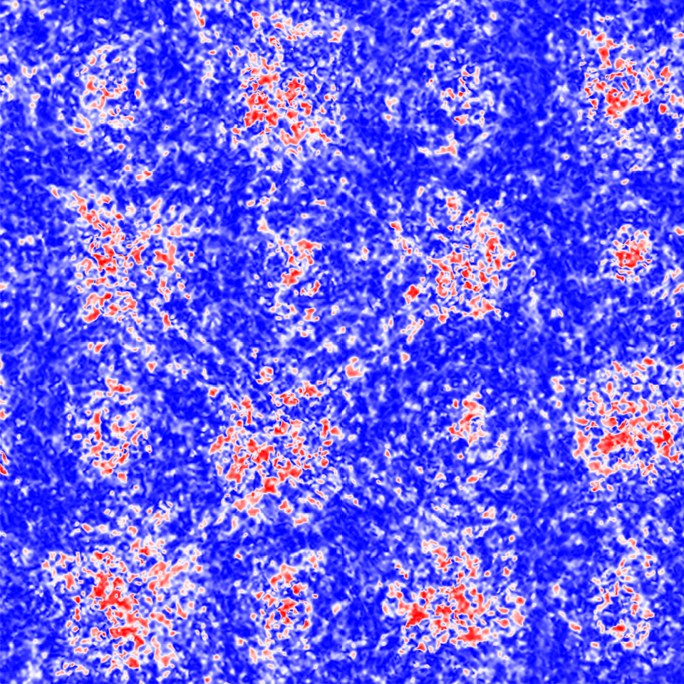
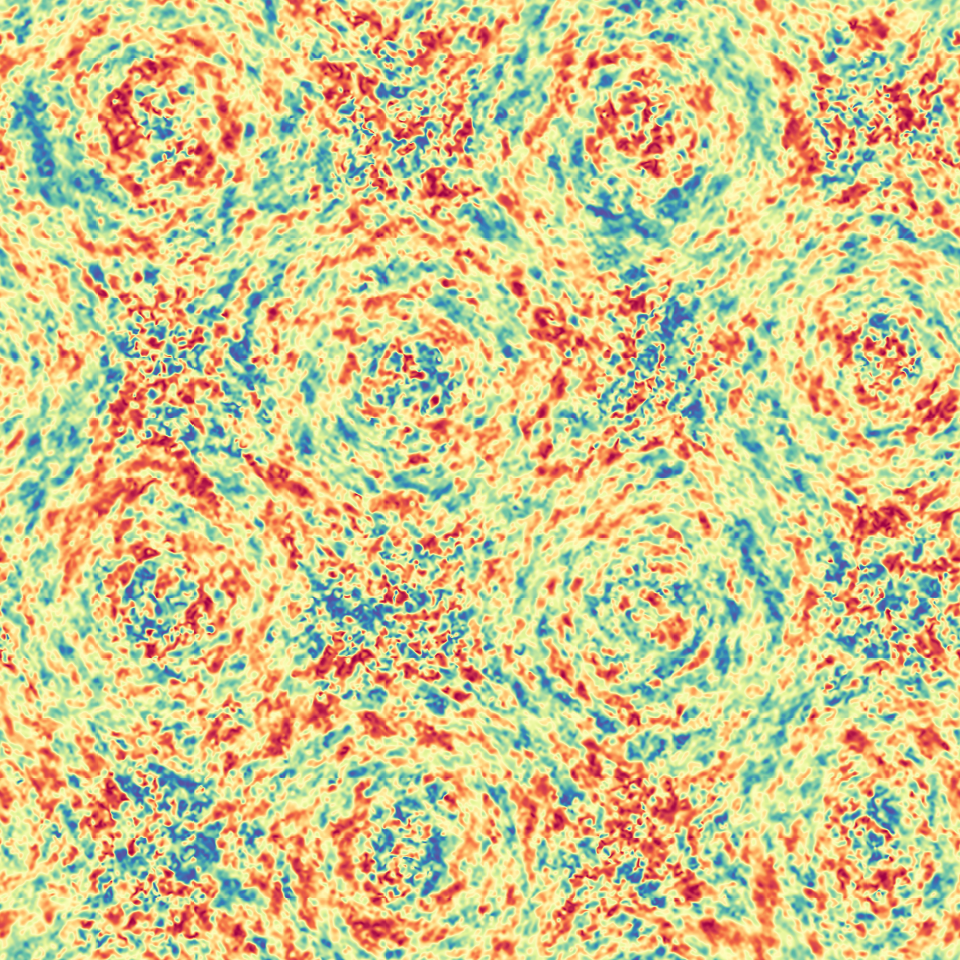
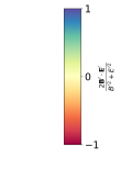
Figure 8: Snapshot at late times of the vector field from the same case with $\lambda/g_{D}^{2}=100$ shown in figures 4 and 5. In the left panel, we show $F^{\prime 2}=2(B^{\prime 2}-E^{\prime 2})$, indicating electric (red) or magnetic (blue) dominance, and in the right panel, we show $\epsilon_{\mu\nu\lambda\rho}F^{\prime\mu\nu}F^{\prime\lambda\rho}=4\mathbf{E}^{\prime}\cdot\mathbf{B}^{\prime}$, indicating the degree to which the electric and magnetic field are aligned or anti-aligned. In both cases, the quantities are normalized by $2\rho_{A^{\prime}}$, so that they are bounded by $\pm 1$.

4.2 Three-dimensional results

Though the above results were obtained assuming a translational symmetry in one spatial dimension (e.g. string vortices are infinitely long), we also perform fully 3D calculations and confirm that our main findings on vortex formation are independent of this assumption. Specifically, we consider a fully 3D case with $\lambda/g_{D}^{2}=25$. We compare this to the equivalent case assuming a translational symmetry in figure 9. There it is evident that the evolution of the energy in the scalar and vector components is similar in the two cases, with the only difference being a faster decay in the vector field energy for the fully 3D case. Though partially a function of finite numerical resolution, a more efficient transfer of energy from the vector to scalar field in 3D is expected since (see section 5.1), with the symmetry assumption, the dark electric field can only accelerate strings in the transverse direction, while without the symmetry assumption, the dark electric field can accelerate strings and the dark electric and magnetic fields can stretch the length of the strings.

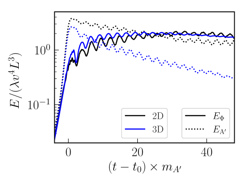
Figure 9: Energy in the scalar field (including interaction energy with the vector; solid lines) and energy in the vector field (not including interaction energy; dashed lines) as a function. We compare two cases with $\lambda/g_{D}^{2}=25$: one where a translational symmetry is enforced in one spatial direction (black lines labelled 2D), and one where on symmetries are enforced (blue lines labelled 3D).

Another difference we find, when not assuming a spatial symmetry, is that intersections between vortex strings efficiently lead to the formation of a large number of smaller scale closed loops, a sign of a fast melting phase transition, analogous to the one discussed in section 2.3, with the mild $\lambda/g_{D}^{2}$ values used in the simulation. This is illustrated in figure 10. Also, in contrast to figure 5, regular dense bundles of vortices are not evident at late times.

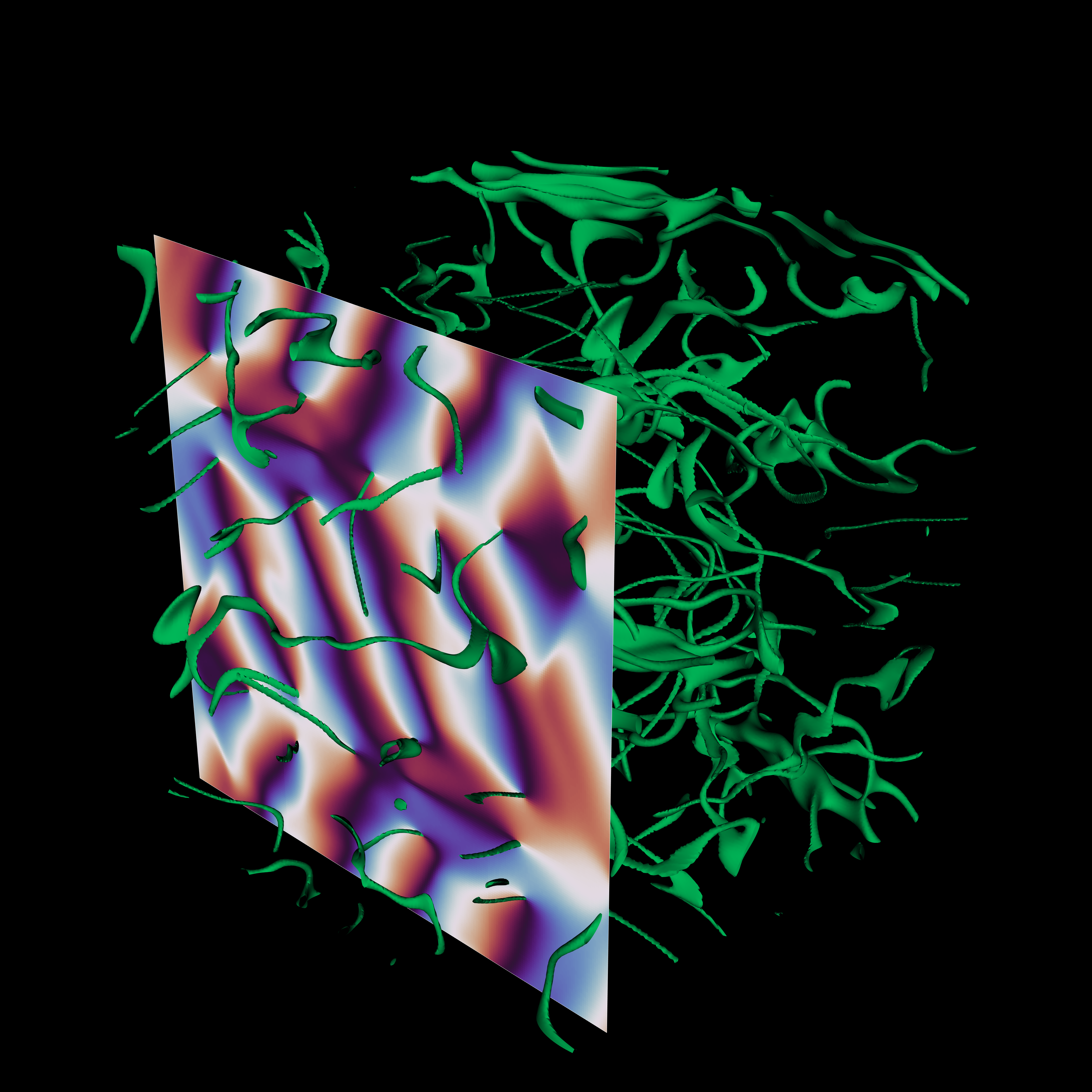
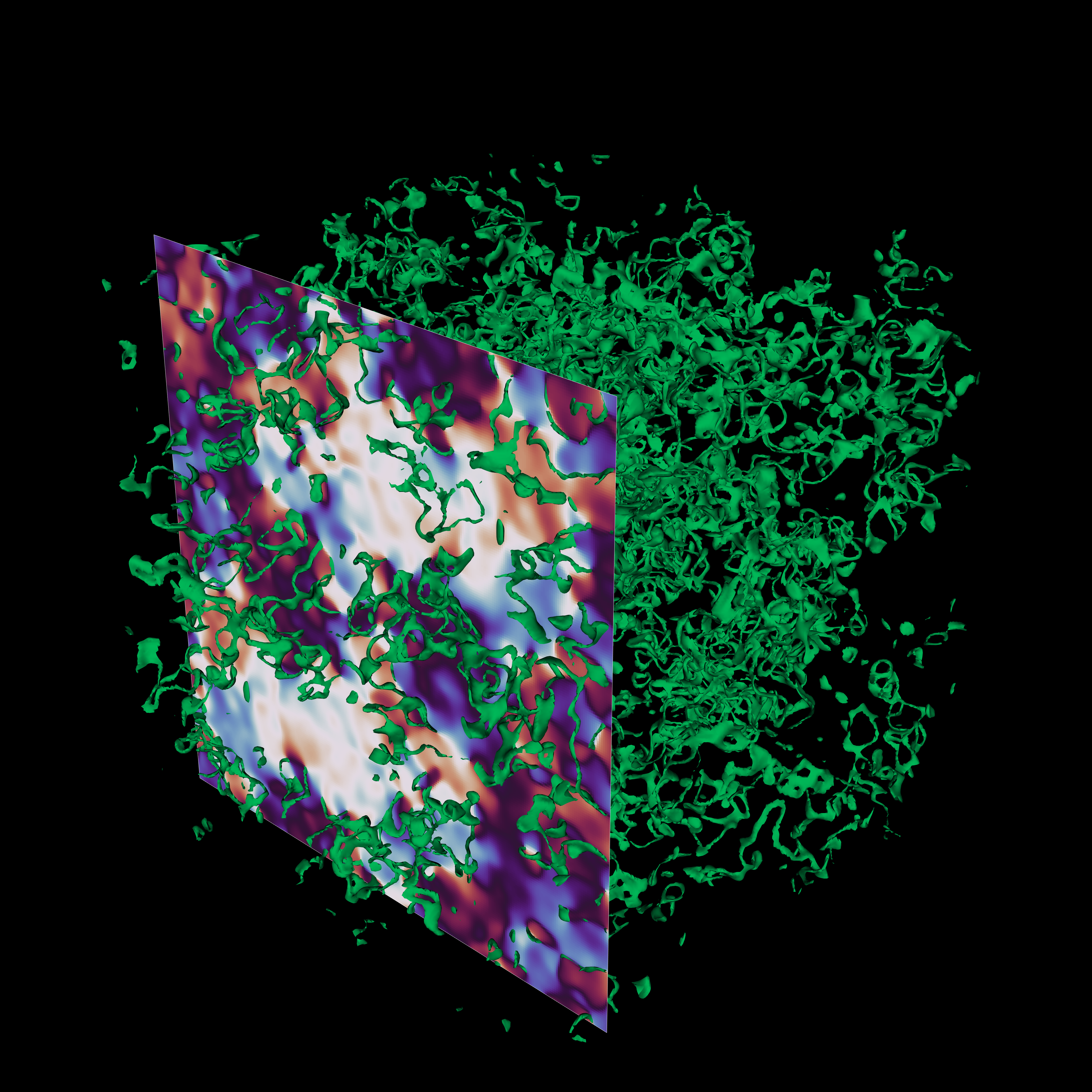
Figure 10: Scalar field from a fully 3D dimensional case with $\lambda/g_{D}^{2}=25$. Contours of $|\Phi|=v/10$ are indicated in green, while the complex phase of $\Phi$ is indicated on a representative two dimensional slice. The left panel shows a snapshot $\approx 3m_{A^{\prime}}$ after vortices first form. The right panel shows a snapshot at a time $\approx 48m_{A^{\prime}}$ after the first, illustrating how reconnections have lead to a larger number of smaller scale loops. The length of the domain is the wavelength of the dominant mode of the axion instability, which is approximately equal to the Compton wavelength of the dark photon ($L=2\pi/k_{p}$ where $k_{p}\approx 1.055m_{A^{\prime}}$).

We find that vortices form when the magnetic field reaches $B^{\prime 2}\sim 2\lambda v^{4}$. This field strength is comparable to the superheating field strength in the Landau-Ginzburg theory, suggesting that the superheating phenomenon occurs regardless of if the initial condition is the Meissner phase, where magnetic field is absent in the bulk, or dark photon dark matter, where the magnetic field already exists in the bulk. A possible explanation is that even in the Meissner phase, within a magnetic penetration depth $1/m_{A^{\prime}}$ from the edge of the superconductor, there is magnetic field with comparable strength to the external magnetic field, and the existence of edges is also not required for the formation of vortices.

5 Evolution post vortex formation

Once vortices form due to the production of a longitudinal or magnetic mode, they will evolve inside the background electromagnetic field. In the case of a type II superconductor, a two-dimensional Abrikosov lattice forms in the background of a uniform, constant magnetic field, and the magnetic field gets confined inside these vortices. In the context of dark matter, this would correspond to moving the energy that is stored in the background dark photon field into the energy of the vortices, which subsequently radiates away a sub-component of their energy into dark photons, and possibly gravitational waves, of much higher energy, depleting the dark photon dark matter.

The post vortex formation evolution of dark photon dark matter differs conceptually from the superconductor case in two ways. Firstly, as mentioned in the context of vortex production, there is not really an edge of the superconductor in the case of dark photon dark matter. Secondly, the strings start in random directions at the time of formation on large scales, but are aligned on small scales. In the case of longitudinal mode production during inflation, these dark photon strings evolve in a manner that is very similar to the case of gauge strings. However, in the case of magnetic mode production in the late universe, there will be a superheating period during the production of magnetic modes, which ends with the rapid formation of strings with length per Hubble patch much larger than the density of a scaling solution. This sets off a period of rapid evolution, during which there is rapid reconnection, and a burst of dark photon and gravitational wave emission.

At formation, assuming that $m_{\rho}\gg m_{A^{\prime}}\sim k_{c}\sim H$, the vortices form as roughly parallel lines with distances of $1/k_{c}$, which evolves eventually to $a_{L}\sim\left(m_{\rho}m_{A^{\prime}}\right)^{-1/2}$ and the energy density of these vortices in their ground state is

$$\rho_{v}\sim v^{2}/a_{L}^{2}\simeq m_{\rho}m_{A^{\prime}}v^{2},$$ (25)

whereas the energy density in the dark photon field before vortex formation is $B^{2}\sim v^{3}m_{\rho}\gg\rho_{v}$, as expected from the superheated nature of the phase transition. On the other hand, the total energy stored in the electric field and magnetic field before the phase transition, even if all converted into thermal energy of the radial mode, can barely reheat the system enough to totally restore the symmetry. Therefore, the evolution of the string network post vortex formation is determined by the effective theory of the vortices interacting with a background dark electromagnetic field.

5.1 Dark electric field in the presence of vortices

When vortices form in a background electromagnetic field, the magnetic field, and hence the magnetic field energy, is concentrated in the vortices, resulting in a highly excited state of vortices. However, in the case of dark photon dark matter, there might still be a significant amount of energy stored in the oscillating dark electric field. In the following, we will give a simple description of the interaction of the vortices with the background electric field and how the electric field is dissipated. To begin, let us consider a vortex line pointing in the z-direction moving in the x-direction with velocity $\boldsymbol{\mathbf{v}}=v_{x}\hat{x}$, as shown in figure 11. The dark electric field outside of the core can be computed as

$$\boldsymbol{\mathbf{E^{\prime}}}=\frac{d\boldsymbol{\mathbf{A^{\prime}}}}{dt}=-\boldsymbol{\mathbf{v}}\cdot\nabla\boldsymbol{\mathbf{A^{\prime}}}$$ (26)

where the spatial vector $\boldsymbol{\mathbf{A}}^{\prime}$ comes from the vortex

$$\boldsymbol{\mathbf{A^{\prime}}}=\frac{1}{2g_{D}}\frac{\hat{\boldsymbol{\mathbf{\theta}}}}{r}$$ (27)

and as a result

$$\boldsymbol{\mathbf{E^{\prime}}}=-\left(\frac{v_{x}\Phi_{D}}{2\pi r^{2}}\right)\left(\hat{\boldsymbol{\mathbf{r}}}\sin\theta-\hat{\boldsymbol{\mathbf{\theta}}}\cos{\theta}\right).$$ (28)

This is the electric field of a dipole in two dimensions with dipole moment of $\boldsymbol{\mathbf{d}}=-v_{x}\Phi_{D}\hat{\boldsymbol{\mathbf{y}}}$, where $\Phi_{D}=\pi/g_{D}$ is the dark magnetic flux quantum. As a result, a vortex moving in an electric field in the y-direction, experiences a force in the same direction, and energy is transferred from the oscillating electric field to the kinetic energy of the vortex. During subsequent collisions of the vortex lines, this kinetic energy can be transferred to potential energy (string length) and the dark electric field energy is dissipated. This is evident in the superradiance simulation in East:2022ppo (discussed in section 7.2), as well as the 3+1d simulation discussed in the previous section.

The vortex dynamics discussed in this section can also be seen easily from the perspective of the particle-vortex duality in $2+1$D Peskin:1977kp , where the electric field in the x-direction is dual to a current in the y-direction in the XY model. In the dual theory, the current in the original theory is dual to the gauge field in the dual theory, and vortices will have velocities of order $E/B$ where $E$ and $B$ are the electric and magnetic field strength before the superheated phase transition.

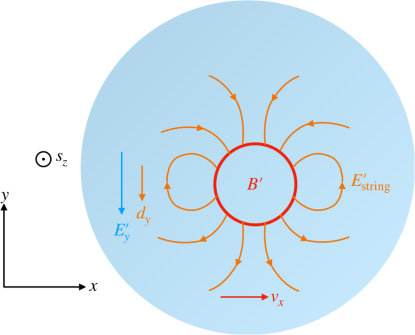
Figure 11: A vortex aligned in the $\boldsymbol{\mathbf{z}}$-direction accelerates inside a background dark electric field $\boldsymbol{\mathbf{E}}^{\prime}$. The moving vertex (red) has a dipole electric field from a dipole moment of $\boldsymbol{\mathbf{d}}=-v_{x}\Phi_{D}\hat{\boldsymbol{\mathbf{y}}}$ (orange). The velocity, and hence the dipole moment, increases to reduce the dipole energy $-\boldsymbol{\mathbf{d}}\cdot\boldsymbol{\mathbf{E}}^{\prime}$.

5.2 Residual field

A moving vortex line aligned in the $z$-direction has a 2D magnetic dipole moment $\boldsymbol{\mathbf{\mu}}=\Phi_{D}\hat{\boldsymbol{\mathbf{z}}}$ and a 2D electric dipole moment $\boldsymbol{\mathbf{d}}=-v_{x}\Phi_{D}\hat{\boldsymbol{\mathbf{y}}}$. Translating to 3 dimensions, we have

$$\frac{d\boldsymbol{\mathbf{\mu}}}{dl}\sim\frac{d\boldsymbol{\mathbf{d}}}{dl}\sim 1/g_{D}$$ (29)

when a section of string is moving relativistically, where $l$ is the length along the string direction. In a background dark electromagnetic field, a section of string experiences a force from the dark electromagnetic field, as well as from the string tension $\mu\sim\pi v^{2}$. The string length, as a result, will increase as long as

$$\frac{d\boldsymbol{\mathbf{\mu}}}{dl}\cdot\boldsymbol{\mathbf{B^{\prime}}}>\pi v^{2},\quad,\frac{d\boldsymbol{\mathbf{d}}}{dl}\cdot\boldsymbol{\mathbf{E^{\prime}}}>\pi v^{2},$$ (30)

when the dark electromagnetic field energy transfers to the energy of the string. Such a process stops when

$$|\boldsymbol{\mathbf{B^{\prime}}}|,\,|\boldsymbol{\mathbf{E^{\prime}}}|\lesssim g_{D}v^{2}.$$ (31)

Note that $g_{D}v^{2}$ is exactly $B_{\rm c1^{\prime}}$, the magnetic field strength when the Abrikosov vortex solution becomes energetically favorable, as we expect. To conclude, in a system that does not have a magnetic field direction that is enforced by an external source and that allows for the dissipation of vortex energy, the background dark electromagnetic field will continue to decreases until it reaches $\mathcal{O}(g_{D}v^{2})$. Such a continues decrease is seen in both simulations in 3D (figure 4 and figure 12). In neither case, however, do we see the field strength decreases to as low as $B^{\prime}_{\rm c1}=g_{D}v^{2}$ in the duration of the simulation. This can be a result of the finite duration of the simulation, as well as the overlapping magnetic field coming from the magnetic flux carried by the vortex itself. In the cosmological case, a full simulation of the vortices with cosmic expansion might distinguish between the two possibilities. We should stress that such dynamics is independent of the origin of the vortex/string and can occur in any growing gauge field in the presence of a defect. We postpone the study of these scenarios to future work.

5.3 A super-scaling network

As described in the previous sections, after exceeding the superheating threshold, most of the coherent dark electromagnetic field gets converted into the string network. This highly excited string network contains energy density that is equal to the electromagnetic energy stored in the coherent field, of order $\lambda v^{4}$, whereas the energy density of a network approaching the scaling solution in a cosmological setting has energy $H^{2}v^{2}\sim g_{D}^{2}v^{4}$. This suggests that at the end of the phase transition, there is a network of strings with $\xi_{i}\approx\lambda/g_{D}^{2}\gg 1$, where $\xi_{i}=\rho_{\rm string}/\mu H^{2}$ measures the total length of the strings in Hubble units, and would be an $\mathcal{O}(1)$ number for a scaling network.

This super-scaling network will quickly approach scaling by emitting dark photons, gravitational waves, and possibly also the radial mode of the Higgs. The exact composition and spectrum of the radiation depends mainly on the dynamics of the melting phase transition. In particular, it depends on if the restoration of the translational symmetry in the direction of the magnetic field happens at the same rate as the restoration in the directions perpendicular to the magnetic field. An $\mathcal{O}(1)$ portion of the vortex energy can be re-emitted into higher energy dark photons, which would redshift to be non-relativistic again, and thus constitute a significant portion of the dark matter. The string network would decay dominantly into high energy ($\omega\gg H\sim m_{A^{\prime}}$) dark photons if the melting transition is fast. On the other hand, if such a melting transition is slow, then the network can decay predominantly into gravitational waves. After the melting phase transition, the super-scaling network approaches the scaling solution Polchinski:2006ee . It is not clear how fast this occurs, which affects the prediction for the gravitational wave and dark photon frequency distribution around the peak frequency. We discuss the phenomenological consequences in section 7.1.

6 Dark photon superradiance cloud

In East:2022ppo , it was demonstrated that string vortices could form as the results of the superradiant instability of a dark photon around a spinning black hole. We begin by briefly summarizing those results. At smaller field values, the dark photon field acts like a Proca field, and grows exponentially in time. Provided the instability does not saturate through gravitational backreaction beforehand, as $|F^{\prime 2}|$ reaches $\sim B^{\prime 2}_{\rm sh}$, string vortices form. The string formation first occurs with a pair of strings orientated longitudinally around the black hole. The dark electric field drives one string into the black hole, and the opposite winding number string outward (as in section 5.1). The latter first grows, with a large portion of the energy originally in the vector field going in the scalar, in particular the kinetic (rotational) and potential energy (length) of the string, and then shrinks, as a combination of the string tension and gravity cause it to collapse back to the black hole horizon. Several strings loops in the vicinity of the black hole horizon are excited, but also eventually fall back into the black hole. Following the transient period where string vortices exist, and a large fraction of the vector cloud is dissipated due to radiation (as well as flux into the black hole), superradiant growth begins again.

In figure 12, we show the field strengths from one of these cases. Comparing to figure 4, we can note several differences in the superradiant instability case versus the axion instability case. In contrast to the axion instability case, the Proca cloud is electrically dominated almost everywhere, and in the regions of magnetic dominance, the field strength is significantly smaller. Another difference is that the superradiant instability rate is much smaller than $m_{A^{\prime}}$ (in contrast to the axion instability, where they are comparable), and the initial formation of vortices, marked by the jump of $\min{|\Phi|}$ from $\approx 0.5v$ to $0$ in figure 12) occurs over a short timescale compared to the instability timescale, which accompanies a similar jump in the magnetic field strength. When this jump occurs, the dark magnetic field strength is below the superheating field strength $B^{\prime}_{\rm sh}$. This suggests that the presence of a stronger background electric field can assist the production of vortices through, we speculate, an instability similar to the one shown in figure 3. The relation to the dynamics studied in Bachas:1992bh and its generalization is unclear.

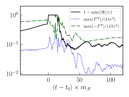
Figure 12: Similar to figure 4, but for a dark photon cloud that arises through superradiance around a spinning black hole. This is the case with dimensionless black hole spin $\chi_{\rm BH}=0.99$, $\alpha\equiv GM_{\rm BH}m_{A^{\prime}}=0.4$, and $\lambda/g_{D}^{2}=25$ from East:2022ppo . We show the displacement from the VEV of the minimum scalar field magnitude (solid black line) around the time when vortices form at $t=t_{0}$. The vortices persist for $\approx 14m_{A^{\prime}}$ and then are absorbed by the black hole. We also show the maximum values of $F^{\prime 2}$ (dotted blue line; corresponding to magnetic dominance) and $-F^{\prime 2}$ (dashed-dotted green line; corresponding to electric dominance).

The characteristic size of the superradiant dark photon cloud is set by $\alpha\equiv GM_{\rm BH}m_{A^{\prime}}$ (where $M_{\rm BH}$ is the black hole mass), and is roughly $1/(\alpha m_{A^{\prime}})$, so the ratio of the cloud size to the the string radius will be set by $\alpha$ and $\lambda/g_{D}^{2}$. The study in East:2022ppo was restricted to cases with $\alpha=0.3$–0.4, and $\lambda/g_{D}^{2}=12.5$–50. For these parameters, only a few string vortices formed (though more were found in the $\alpha=0.3$ versus the $\alpha=0.4$ case at fixed $\lambda/g_{D}^{2}$). However, we can expect that the dynamics will be much more complicated as one increases the ratio $\lambda/g_{D}^{2}$, and that in particular more strings will be formed as the scale separation between the radial mode mass and the dark photon mass is increased, since we do not expect the presence of strings to impede the formation of new vortices in the superradiance cloud Ramos:2005yy .

Though it is not computationally feasible to numerically simulate the $\lambda/g_{D}^{2}\rightarrow\infty$ limit, we can estimate the number of vortices that would be formed in the superradiance cloud in this regime using the results outlined in section 2. From there, vortices are expected to form with a separation on the order of $\sqrt{\pi/g_{D}B^{\prime}}\sim\sqrt{\pi/g_{D}\lambda^{1/2}}/v$, while the superradiance cloud has a radius of order $1/\alpha m_{A^{\prime}}\sim 1/\alpha g_{D}v$. Therefore the number of vortices in the cloud in the limit of large $\lambda/g_{D}^{2}$ and small $\alpha$ is roughly

$$N=c_{1}\frac{1}{\pi\alpha}\sqrt{\lambda/g_{D}^{2}}/\log[\lambda/g_{D}^{2}]\ .$$ (32)

The coefficient $c_{1}$ is an $\mathcal{O}(1)$ constant that depends mainly on the geometry of the system. Note that this scaling might not be very accurate when $\lambda/g_{D}^{2}$ is only moderately large, especially around a black hole with $GM_{\rm BH}\sim a_{L}$.

As an illustrative example, consider a $60\ M_{\odot}$ black hole that is rapidly spinning and a dark photon with mass $m_{A^{\prime}}\simeq 10^{-12}$ eV. Then vortex formation will happen before superradiance saturates due to black hole spin down if $v\lambda^{1/4}\lesssim 10$ MeV. This means that the ratio

$${\lambda/g_{D}^{2}}\lesssim\lambda^{1/2}\left(\frac{10\,{\rm MeV}}{10^{-12}\,{\rm eV}}\right)^{2}=\lambda^{1/2}10^{38}$$ (33)

can be extremely large, in particular if $\lambda$ is order unity. If, on the other hand, one considers very small $\lambda$ (and even smaller $g_{D}$), $\lambda/g_{D}^{2}$ does not have to be humongous, and the energy scale of $v$ can be much larger. We note that if one sets the maximum energy density of the dark photon cloud at gravitational saturation equal to $\lambda v^{4}$, this gives $v\sim\alpha^{5/2}(g_{D}/\lambda^{1/2})m_{\rm Pl}$, independent of the black hole mass. The different choices for the energy scale $v$ will result in different phenomenology for the vortex strings, as we discuss below.

6.1 Evolution post vortex formation in the large ${\lambda/g_{D}^{2}}$ limit

For a superradiance cloud that has fully grown, the quantity ${\lambda/g_{D}^{2}}$ can be as large as $10^{38}$, which corresponds to the formation of $\mathcal{O}(10^{19})$ vortices around a single solar mass black hole. Analogous condensed matter systems in the large ${\lambda/g_{D}^{2}}$ limit exhibit a melting phase transition after the superheated phase transition, though it is unclear in our case how fast the phase transition occurs and if all translational symmetries are restored at the same time. Though such dynamics was not observed for the moderate values of $\lambda/g_{D}^{2}$ considered in East:2022ppo , where only a few strings form in the superradiance cloud, we can expect similar behavior at more extreme values, with a large number of strings interacting in the presence of the time dependent dark electric field, creating loops of irregular sizes.

In a type II superconductor, the melting phase transition eventually completes, and full translational symmetry is restored. This is also the expectation for dark photon dark matter. In the dark photon superradiance cloud, however, the situation is much more complicated. Firstly, the superradiance cloud, and hence the resulting network of vortices, is localized around the black hole by gravity, instead of being nearly uniformly distributed over the whole Higgsed phase. Secondly, most of the energy is initially stored in the dark electric field, which can eject loops that are created before total thermalization/melting occurs (see section 5.1). In figure 13, we sketch how string intersections could create loops that do not encompass the black hole, with a fraction of these being accelerated to relativistic velocities by the dark electric field, and becoming gravitationally unbound, while others fall back into the black hole.

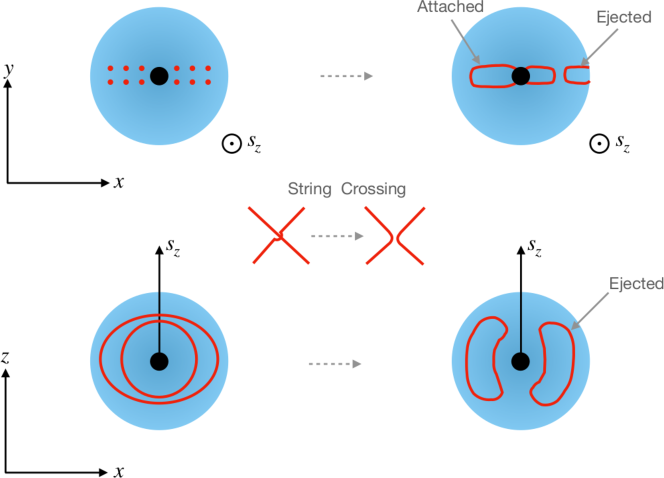
Figure 13: An illustration of how the dynamics of crossings (middle panel) affect the motions string vortices in a dark photon cloud that arose through superradiance around a spinning black hole. Vortices (red dots and lines) form in the dark photon superradiance cloud (blue shaded region) around a spinning black hole (black dot) with spin direction $s_{z}$. Upper panel ($x-y$ plane): Initially parallel strings in the vortex lattice exchange partners with each other, leading to strings that attach to the black hole at different longitudes as well as strings that are ejected. Lower panel ($x-z$ plane): A different configuration where string loops spanning a longitudinal line exchange partners with each other, forming loops that can be ejected from the superradiance cloud.

6.2 Superradiance cloud as a string factory

The initial superheated phase transition produces vortex strings with length on the order of the size of the superradiance cloud $1/(\alpha m_{A^{\prime}})$ as demonstrated in East:2022ppo . These vortex loops will expand due both to the background dark electric field, as well as the repulsive interactions between the vortices when $\sqrt{\lambda/g_{D}^{2}}\gg 1$. These interactions likely make the vortex lines highly irregular before they can escape the superradiance cloud. However, due to geometric string-string interactions, string loops oriented longitudinally around the black hole are also unlikely to have lengths that are much longer than $1/(\alpha m_{A^{\prime}})$ when they escape the region.

Assuming an order one fraction of the total string length escapes the black hole during a stringy bosenova event and an $\mathcal{O}(1)$ quartic coupling, the total number of string loops with $L_{\rm loop}\sim 1/(\alpha m_{A^{\prime}})$ ejected can be up to

$$N_{\rm max}\approx\frac{1}{\pi v^{2}L_{\rm loop}}\int|\boldsymbol{\mathbf{E}}^{\prime}|^{2}dV\simeq\frac{1}{\alpha^{2}}\frac{\lambda}{g_{D}^{2}}\approx 10^{39}.$$ (34)

if we accounted for the assisted pair production in the larger dark electric field seen in the simulation. If we assume the dark magnetic field crosses the superheating threshold, this $\alpha$-scaling would be $1/\alpha^{4}$. These irregular loops can radiate both longitudinal mode dark photons, as well as gravitational waves, losing energy and eventually circularizing. The circularized loops can only radiate into gravitational waves with power $P\sim\Gamma G\mu^{2}$, and hence have a lifetime

$$t\simeq\frac{1}{\Gamma Gv^{2}\alpha m_{A^{\prime}}}\gg t_{\rm age}$$ (35)

where $\Gamma$ is an $\mathcal{O}(50)$ constant, $\mu$ is the string tension, and $t_{\rm age}$ is the age of the universe Hindmarsh:1994re . Here, the main uncertainty comes from a lack of understanding of the melting transition for a superradiant cloud, and, as a result, uncertainty regarding the spectrum of the dark photon strings emitted.

The strings themselves are capable of superradiance Frolov:1995vp ; Kinoshita:2016lqd ; Igata:2018kry , which opens the possibility that after the the initial burst of string production when the dark photon cloud grows sufficiently large, the strings can continue to grow in number/length by extracting energy and angular momentum from the spinning black hole. Xing et al. Xing:2020ecz describes a scenario where a string whose ends are attached to the black hole horizon at different longitudes could exhibit a type of superradiant instability, where tension modes would be amplified by successive reflections by the horizon. (Though the treatment there was non-relativistic, and the role of reconnections and the saturation of such an instability was left open.) Following a stringy bosenova event, a significant portion of the irregular strings that fall towards the black hole may intersect the horizon in configurations that enables them to continue to extract energy and angular momentum from the black hole. (This is in contrast to what was found in simulations with a small number of strings East:2022ppo , where the strings that intersected the black hole had both ends attached at approximately the same longitude and were not long-lived.) The rate of energy extraction per string is set by the string tension $\mathcal{O}(v^{2})$ Kinoshita:2016lqd ; Igata:2018kry ; Xing:2020ecz . Such an energy extraction rate is much smaller than the superradiance rate of a full superradiance cloud. However, given the huge number of strings that are produced, and subsequently attach to the black hole horizon, it is possible that such an energy and angular momentum extraction rate is enhanced by the $\mathcal{O}(\sqrt{\lambda/g_{D}^{2}})$ number of strings attached to the black hole, beyond which point the string cores start to overlap with each other.

These strings that intersect the black hole horizon might continuously extract energy from the black hole through string superradiance. However, a visible signal from string superradiance would require a huge numbers of strings extracting energy from the black hole at the same time. On the other hand, one or more strings could impede the superradiant growth of a dark photon, assuming that the dark photon cloud loses energy by accelerating the strings (section 5) at a greater rate than it extracts energy from the spinning black hole. The phenomenological consequences of these vortices will be discussed in section 7.2.

7 Phenomenology

The main phenomenological consequences of the dynamics studied in this paper are the early depletion of dark photon dark matter and dark photon superradiance clouds through vortex formation. The energy that is transferred to string networks, however, opens up new phenomenological possibilities. In the case of vortex formation in the early universe, the dense network of string would have already decayed away, and we can look for the indirect evidence of their existence through their gravitational wave signals. In the case of vortex formation from black hole superradiance, there are direct signals coming from vortex lines ejected by the black hole.

7.1 Gravitational waves from dark photon dark matter

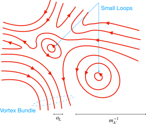
Figure 14: A schematic view of the vortex network generated after a superheated phase transition, but before the melting phase transition is complete. The long vortex lines have length $L\gtrsim m_{A^{\prime}}^{-1}$ and relatively uniform direction on scales of order $m_{A^{\prime}}^{-1}$, forming a vortex bundle. The vortex line separation is of order $a_{L}$, the lattice spacing. The long vortex bundle emits gravitational waves with frequency $\omega\sim 1/L$, while the small string loops disappear quickly into high energy dark photon longitudinal modes with $\omega\sim 1/a_{L}$.

In the case of inflationary dark photon production, the vortices formed during inflation will quickly evolve into a scaling solution of cosmic strings after reheating if the Hubble scale is larger than the scale $v$. If $v\gtrsim H_{\rm I}$, however, the dynamics can differ from the formation of Nambu-Goto strings NambuGoto . Unlike Nambu-Goto strings, which can only shrink in total length after they enter the horizon, the length of dark photon strings can continue to grow as strings enter nearby Hubble patches which contain a dark electromagnetic field. This allows the string network to evolve into scaling even if the original exponentially suppressed production during inflation cannot produce enough strings to enter a scaling regime. We leave a more in-depth study to future work.

In the case of late time production mechanisms for the dark photon, vortices are produced in a superheated phase transition as the dark electromagnetic field grows. These strings form a super-scaling network, with an effective $\xi_{i}\gtrsim\sqrt{\lambda/g_{D}^{2}}$. After formation, the string length can continue to grow inside the background dark electric field to a total length of string that corresponds to at most $\xi_{i}\lesssim\lambda/g_{D}^{2}$.

After an initial transient phase, the background dark electromagnetic field is dissipated, and the strings will continue to evolve via string-string interactions towards a scaling network. The system differs from the standard picture in two ways. Firstly, there are a large number of defects in a single Hubble patch, similar to the string network after a second order phase transition KIBBLE1980183 ; zurek1985cosmological ; Kibble:1997yn . Secondly, the network, before the melting phase transition is complete, breaks translational symmetry and is maximally anisotropic on Hubble scales, and this anisotropy can be long-lived since the densely packed strings have a significant repulsion between them.

The phenomenological consequences mainly depend on whether the emission from the string network is determined by the behavior of individual string loops, or by the collective behavior of bundles of strings (see figure 14 for a schematic view of the string network). The bundle of long strings will emit significant gravitational radiation at a frequency corresponding to the inverse of the length of the strings (comparable to Hubble scale at that time). On the other hand, if the melting transition takes place efficiently after the formation of the strings, then most of the energy will go into longitudinal dark photons, which have a frequency of order $1/a_{L}$ (inverse lattice spacing) as long as $1/a_{L}$ is larger than the dark photon mass. It is unclear how this network approaches a scaling solution, and as a result, our projections for the emission, shown in figures 15 and 16, should only be regarded as crude estimates.

In both figure 15 and figure 16, we assume that there is no initial seed of strings produced in the early universe, and that the length of cosmic string starts decreasing rapidly after the phase transition. The former assumption is equivalent to $H_{I}\ll v$, since the growth of a dark photon dark matter field will be halted by the presence of seed vortices. The latter is a good approximation when the string network forms quickly, and dissipates its energy mainly into longitudinal dark photons at $\omega\sim 1/a_{L}$ (see Long:2019lwl for more details). In this case, most string loops, after the melting phase transition, have length in the range

$$\frac{1}{m_{\rho}}\ll L_{\rm loop}\ll\frac{1}{m_{A^{\prime}}}$$ (36)

and the behavior of the string network is the same as an axion string network until $\xi_{i}$ drops to be $\mathcal{O}(1)$. On the other hand, if the string network dissipates a large portion of its energy before the melting phase transition is complete, then it is possible that the energy released into gravitational waves is low. The main uncertainty in estimating the gravitational wave power comes from the effect of interference. If the bundle of strings emit gravitational wave independently, then the emission power scales linearly with $\xi_{i}$, and the lifetime of strings with length $L>1/m_{A^{\prime}}$, much longer than the Hubble scale when the string network forms, is $\mathcal{O}(L/Gv^{2})$ due to gravitational wave emission. In this case, the string network will predominantly emit dark photons after the melting transition is complete. However, if a bundle of strings oscillates and emits gravitational waves coherently before the melting phase transition is complete, then the emission power scales quadratically with $\xi_{i}$, and the lifetime of long strings is $\mathcal{O}(L/G\xi_{i}v^{2}\sim L)$ due to gravitational wave emission, and $\mathcal{O}(1)$ of the energy can be released before the melting phase transition is complete. Simulations of a super-scaling network of gauged strings with anisotropic initial conditions would help make a more precise prediction of the phenomenological consequences.

In both figures, we assume the energy density that is transferred into gravitational wave or dark photon dark matter radiation is $\mathcal{O}(\lambda v^{4})$ at the phase transition, which happens when vortices form quickly, and shut off the exponentially growing gauge field. It is possible that a small amount of energy is continuously pumped into the dark gauge field post string formation. In this case, there might be a significant blue tail to the gravitational wave spectrum since the correlation length of the magnetic field is $\mathcal{O}(1/m_{A^{\prime}})$, which remains relatively constant until the melting transition is complete.

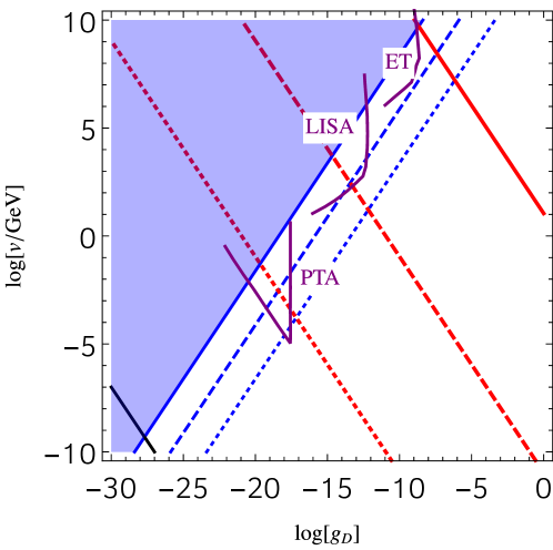
Figure 15: The observational consequence of a network of string bundles that radiates predominantly gravitational waves. The blue shaded region is excluded by constraints on the gravitational wave energy density from the measurement of the effective number of neutrino species $N_{\rm eff}$ Planck:2018vyg , corresponding to dark photon dark matter overclosing the universe before the dynamics we discuss here take place. The blue dashed and dotted lines are $N_{\rm eff}$ of $10^{-5}$ and $10^{-10}$. The red solid, dashed, and dotted lines show the peak frequency of the gravitational wave of kilohertz, millihertz, and ${\rm yr^{-1}}$, respectively. We also show corresponding near term projections for some future gravitational wave detectors (ET, LISA, and a pulsar timing array with SKA, respectively) as solid purple curves Moore:2014lga . Below the black solid line, the dynamics we discuss here occurs after matter-radiation equality.

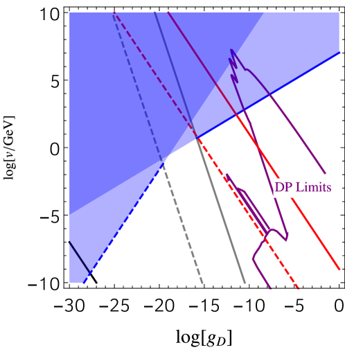
Figure 16: The observational consequences of a network of string bundles that radiates predominantly longitudinal mode dark photons. The blue shaded region is excluded by overclosing the universe on the right, and $N_{\rm eff}$ constraints on the left Planck:2018vyg . The blue solid line is when dark photons make up all of dark matter, while the blue dashed line corresponds to when relativistic dark photons have the same energy density as photons today. The red solid and dashed lines correspond to when the mass of the dark photon is ${\rm eV}$ and ${\rm GHz}$ ($\sim 10^{-6}$ eV), respectively. The gray solid and dashed lines show when the dark photon radiation becomes non-relativistic at, respectively, cosmic temperatures of $T_{\gamma}={\rm keV}$ and today. In the region between the gray solid and dashed lines, dark photon radiation becomes non-relativistic during the time of CMB and structure formation, and the constraint depends on the details of the spectral shape of dark photons emitted by the string network. Below the black solid line, the dynamics we discuss here occur after matter-radiation equality. The parameter space to the bottom right of the purple solid line is excluded by the existing solar, CMB, and ADMX constraints AxionLimits if the kinetic mixing is generated at one loop as in Holdom:1985ag , i. e.  $\epsilon=eg_{D}/16\pi^{2}$.

7.2 Stringy bosenova

7.2.1 Dark magnetic flux tube

Unlike vortex formation in the early universe, where an indirect relic gravitational wave signal can be produced, in the case of a dark photon superradiance cloud, one can hope to directly observe vortex lines that are ejected from the black hole. Taking dark photon masses corresponding to superradiance of black holes with masses in the range $10$ to 100 $M_{\odot}$ (see figure 17), assuming $\lambda=1$, and taking $v$ to be the maximum value where vortex formation happens before black hole spin down halts superradiance (i.e. setting $\lambda v^{4}$ equal to the maximum energy density of the cloud), we arrive at the following parameteric scales. Each vortex loop has a core size $1/(\lambda^{1/2}v)$ of order ${\rm pm}\sim{\rm fm}$, a thickness ($1/{m_{A^{\prime}}}$) (region containing magnetic field) of order $10\sim 10^{4}\,{\rm km}$, and a length ($\sim 1/{\alpha m_{A^{\prime}}}$) of order $10^{2}\sim 10^{6}\,{\rm km}$. We note that for lower values of $\alpha\lesssim 0.1$, it is possible that energy emission from nonlinear interactions halts the superradiant growth of the cloud before the superheating field strength is every reached Fukuda:2019ewf ; East:2022ppo . However, numerical simulations are required to locate the threshold value of $\alpha$ below which this occurs.

A fraction of these loops, after escaping from the superradiance cloud, diffuse into the galaxy. The flux of dark photon strings from a black hole in the galaxy is

$$F_{\rm max}=\frac{N_{\rm max}}{4\pi d^{2}\Delta t}\approx\frac{10^{10}}{A_{\rm string}}{\rm yr}^{-1}\left(\frac{10\,{\rm kpc}}{d}\right)^{2}\left(\frac{10^{5}\,{\rm yr}}{\Delta t}\right),$$ (37)

where $A_{\rm string}=\alpha^{-1}m_{A^{\prime}}^{-2}$ is the effective area of the vortex line, $\Delta t$ is the range of arrival times/duration of semi-relativistic string loops from a distance $d\sim 10\,{\rm kpc}$, and $N_{\rm max}$, the maximal number of strings diffusing out of the black hole superradiance cloud in each bosenova event, is shown in figure 17. This is an enormous flux. In fact, the magnetic field from different strings will still overlap after the strings have diffused from the kilometer-scales of the black hole superradiance cloud to the kiloparsec-scales of the galaxy. After the initial burst, string superradiance Xing:2020ecz may continue to produce string loops out of the black hole. This steady flux can be as large as

$$F_{\rm steady}\sim\frac{N_{\rm max}}{4\pi d^{2}t_{\rm age}}\approx\frac{10^{5}}{A_{\rm string}}{\rm yr}^{-1}\left(\frac{10\,{\rm kpc}}{d}\right)^{2},$$ (38)

if the source black hole is within our galaxy and a large number of strings are attached to the black hole.

Each vortex carries one flux quantum $\Phi_{D}=\pi/g_{D}$. If the dark photon is kinetically mixed with our photon, such a dark magnetic flux will be a visible magnetic flux of $\Phi_{\rm visible}=\pi\epsilon/g_{D}$ where $\epsilon$ is the dimensionless kinetic mixing parameter. The effective magnetic field around a string is

$$B=\frac{\Phi_{\rm visible}}{\pi/m_{A^{\prime}}^{2}}=\epsilon m_{A^{\prime}}v\simeq 10^{-15}\,{\rm T}\left(\frac{\epsilon}{10^{-7}}\right)\left(\frac{m_{A^{\prime}}}{10^{-12}\,{\rm eV}}\right)^{13/4}\left(\frac{M_{\rm BH}}{10\ M_{\odot}}\right)^{7/4}.$$ (39)

A string that is moving at close to the speed of light would intersect the detector for $\mathcal{O}(10^{-2})$ seconds. Current magnetometers can be used to look for such a transient signal PhysRevLett.89.130801 .

If the kinetic mixing parameter is generated at one loop order, then

$$\frac{\Phi_{\rm visible}}{\Phi_{0}}=\frac{e\epsilon}{g_{D}}=\frac{e^{2}g_{D}}{16\pi^{2}g_{D}}=\frac{\alpha_{\rm EM}}{4\pi},$$ (40)

where $\alpha_{\rm EM}=e^{2}/(4\pi)\approx 1/137$ is the fine structure constant. Such a quantised magnetic flux, spread over an area of order ${\rm km^{2}}$, has magnetic field strength of order $10^{-26}\,{\rm T}$, and is beyond the sensitivity of current experiments. One way to enhance the signal is to have a string that carries a large number of magnetic flux quanta. This is, however, very unlikely, since the force between fluxes are repulsive in the limit of large $\lambda/g_{D}^{2}$.

Figure 17: Maximum number of vortex lines (left axis) and equivalent flux (in units of inverse light seconds squared per year, right axis) emitted in a stringy bosenova as a function of the dark photon mass. The solid and dashed lines correspond to black holes with masses of $10$ and $100M_{\odot}$, respectively, with dimensionless spin $\chi_{\rm BH}=0.5$ when the stringy bosenova event happens. We take the quartic $\lambda=1$, and assume that the dark photon superradiance grows until the black hole spins down by $\Delta\chi_{\rm BH}=0.1$ for the azimuthal number $m=1$ mode, and that the black hole was formed $10^{6}\,{\rm years}$ ago.

Finally, in passing, we note that the large number of vortices, if formed and ejected from the black hole with relativistic velocities, will inevitably travel from galaxy to galaxy, and be captured by black holes in different galaxies Xing:2020ecz . This has an amusing effect of “infecting” the black holes the strings encounter. A vortex string that is attached in a superradiating mode could then hinder vector superradiance as long as it is attached. In certain cases, this means that vector superradiance might not be occurring due to the existence of these persisting strings, as light and as insignificant as they may be compared to the black hole they are attached to . These strings might track their origin back to an earlier stringy bosenova event, or some early universe vortex production through either Kibble mechanism KIBBLE1980183 , or the mechanisms we discussed in this paper. We leave a detailed study of this scenario to future work.

7.2.2 Gravitational wave sirens

If we assume the condition for the assisted superheated phase transition $|\boldsymbol{\mathbf{E}}^{\prime}|\simeq B^{\prime}_{\rm sh}$ (as seen in seen in the superradiance simulations) is satisfied just below when the dark photon cloud reaches the maximum density allowed by black hole spin down, then we have

$$|\boldsymbol{\mathbf{E}}^{\prime}|^{2}\simeq\alpha^{5}m_{A^{\prime}}^{2}/G=\lambda v^{4}\rightarrow\frac{\lambda}{g_{D}^{2}}\simeq\frac{\alpha^{5}}{Gv^{2}}.$$ (41)

Thus strings with tension as large as $G\mu=\pi\alpha^{5}g_{D}^{2}/\lambda$ can be produced and ejected from the black hole in a stringy bosenova event (up to logarithmic corrections). We consider here the case where the quartic coupling $\lambda$ is very small, and $\lambda/g_{D}^{2}$ is only moderately large. For $\alpha\approx 0.3$ and $\lambda/g_{D}^{2}\sim 10^{3}$,

$$G\mu\simeq 10^{-5}\left(\frac{\alpha}{0.3}\right)^{5}\left(\frac{10^{3}}{\lambda/g_{D}^{2}}\right),$$ (42)

suggesting that the stringy bosenova event can lead to the production of strings that are impossible even in the very early universe. In fact, CMB measurements suggest that strings produced in the early universe must have tension $G\mu\lesssim 10^{-7}$ Charnock:2016nzm . However, since a stringy bosenova event only produces very short string loops at late times, none of the strong limits for the early universe apply.

After production, we expect a fraction of the string loops to be ejected from the black hole, emitting radiation at first predominately in gravitational waves, and subsequently in dark photons. The lifetime of such a string loop is

$$t_{\rm life}\sim\frac{1}{\Gamma G\mu\alpha m_{A^{\prime}}}\sim\frac{\lambda/g_{D}^{2}}{\Gamma\alpha^{6}m_{A^{\prime}}}=6\,{\rm kyr}\left(\frac{\lambda/g_{D}^{2}}{10^{13}}\right)\left(\frac{0.3}{\alpha}\right)^{6}\left(\frac{10^{-12}\,{\rm eV}}{m_{A^{\prime}}}\right).$$ (43)

Two qualitatively different regimes exists: one where the strings have a lifetime much shorter than the travel time between the source and the earth, and one where the lifetime is much longer. For the former, all $N_{s}=\lambda/(g_{D}^{2}\alpha^{2})$ strings decay close to the source black hole, which produces a burst of gravitational wave with duration $t_{\rm life}$, characteristic frequency $\alpha m_{A^{\prime}}$, terminal frequency $m_{A^{\prime}}$ (when the dark photon longitudinal mode emission dominates the energy loss) and roughly a strain

$$h\sim\frac{1}{m_{A^{\prime}}^{3/2}t_{\rm life}^{1/2}d}=4\times 10^{-18}\left(\frac{\alpha}{0.3}\right)^{3}\left(\frac{1000}{\lambda/g_{D}^{2}}\right)^{1/2}\left(\frac{10^{-12}\,{\rm eV}}{m_{A^{\prime}}}\right)\left(\frac{10\,{\rm kpc}}{d}\right)$$ (44)

where $d$ is the distance from us to the source. On the other hand, if the strings have a lifetime much longer than the travel time between the source of the string and the earth, then the string loops behave as gravitational sirens, flying around in the galaxy and possibly the universe while emitting gravitational waves. For the string that gets closest to the earth en route within an observing time $t_{\rm obs}\ll t_{\rm life}$, the typical distance between it and the earth is $D_{s}\sim\sqrt{d^{3}/N_{s}t_{\rm obs}}$. This string generates a strain of

$$h\sim\frac{\Gamma^{1/2}G\mu}{\alpha m_{A^{\prime}}D_{s}}=3\times 10^{-26}\left(\frac{\alpha}{0.3}\right)^{3}\left(\frac{10^{12}}{\lambda/g_{D}^{2}}\right)^{1/2}\left(\frac{10^{-12}\,{\rm eV}}{m_{A^{\prime}}}\right)\left(\frac{10\,{\rm kpc}}{d}\right)^{3/2}\left(\frac{t_{\rm obs}}{10\,{\rm year}}\right)^{1/2}.$$ (45)

Such a signal has a much longer duration, and signals from strings from different black holes can overlap in time. In the limit $t_{\rm life}\gg t_{\rm age}$, the universe is filled with small string loops with density $N_{s}n_{\rm BH}$, emitting gravitational waves at the same time. Here $n_{\rm BH}$ is the number density of black holes that have underwent a stringy bosenova event. Gravitational lensing can also be used to look for these light massive objects Dai:2019lud ; VanTilburg:2018ykj . In addition to the gravitational wave emission, the string loops also produces a large amount of dark radiation in the form of longitudinal dark photons. We leave a more detailed study to future work. Lastly, given the large tension, these strings could also extract energy from black holes much more efficiently through string superradiance Xing:2020ecz , which can potentially lead to strings that are longer than the ones we considered in this section getting ejected from the black hole.

8 Remarks

In this paper, we point out how the formation of string vortices and the ensuing nonlinear dynamics can significantly affect the validity of various dark photon dark matter production mechanisms. These dynamics, however, introduce new phenomenological opportunities. The direct and indirect signals from vortex formation and evolution in both dark photon dark matter and dark photon superradiance clouds can be looked for with gravitational wave detectors, dark photon detectors, as well as magnetometers.

It is evident that the relative strength of the main observational signals of our study depends strongly on understanding the melting phase transition, that is the transition to a large number of vortex strings that are uncorrelated on large scales, which has been an active research area of condensed matter physics  zeldov1995thermodynamic ; james2021emergence ; liu1991kinetics ; PhysRevB.8.3423 . A better understanding of how this phase transition takes place following a superheated phase transition in the large $\lambda/g_{D}^{2}$ limit will be important for narrowing down the uncertainties.

In a large portion of the parameter space for dark photon dark matter where $v\lesssim H_{I}$ or $v\lesssim T_{\rm RH}$ (the reheating temperature), we would be left with a large number of strings from prior phase transitions, as well as the dynamics described in this paper. The existence of these strings can impede the growth of coherent field in the late universe. In the background of these defects, coherent fields growing past the critical field $B^{\prime}_{\rm c1}=g_{D}v^{2}$ (and electric field of a similar order) can already be damped by the strings. Understanding the details of this effect, which we leave to future work, can be important in the context of vector black hole superradiance, dark matter dynamics in galaxy mergers, and the constraints on the photon mass Adelberger:2003qx .

Besides the dark photon dark matter and dark photon superradiance cloud scenarios covered in this work, similar vortex dynamics may potentially occur in a gauge boson cosmological collider wang2020gauge , or dark matter scattering during galaxy mergers Lasenby:2020rlf . In some of these cases, the dynamics described in this paper, and the subsequent evolution of the string networks, can lead to other striking signals. We leave these studies to future work.

Appendix A Abelian Higgs Simulations

As in East:2022ppo , we numerically solve the Abelian-Higgs equations of motion in the Lorenz gauge ($\partial_{\mu}A^{\prime\mu}=0$) using $\Phi=\Phi_{R}+i\Phi_{I}$, $\partial_{t}\Phi$, $A^{\prime}_{\mu}$, and $E^{\prime}_{i}\equiv F^{\prime}_{it}$ as our evolution variables. With these variables, the evolution equations take the following form:

$$\partial_{t}^{2}\Phi = \partial_{i}\partial^{i}\Phi-2ig_{D}A^{\prime\mu}\partial_{\mu}\Phi-g_{D}^{2}A^{\prime\mu}A^{\prime}_{\mu}\Phi-\lambda(|\Phi|^{2}-v^{2})\Phi,$$ (46)

$$\partial_{t}A^{\prime}_{i} = -E^{\prime}_{i}+\partial_{i}A^{\prime}_{t},$$ (47)

$$\partial_{t}A^{\prime}_{t} = \partial_{i}A^{\prime i}-Z,$$ (48)

$$\partial_{t}E^{\prime i} = B^{\prime i}\tau_{a}^{-1}(t)+\epsilon^{ijk}\partial_{j}B_{k}+g_{D}^{2}|\Phi|^{2}A^{\prime i}-g_{D}\left(\Phi_{R}\partial^{i}\Phi_{I}-\Phi_{I}\partial^{i}\Phi_{R}\right)+\partial^{i}Z,$$ (49)

$$\partial_{t}Z = -\sigma Z+\partial_{i}E^{i}-g_{D}^{2}|\Phi|^{2}A_{t}+g\Phi_{R}\partial_{t}\Phi_{I}-g\Phi_{I}\partial_{t}\Phi_{R}.$$ (50)

Here, following Zilhao:2015tya ; East:2017mrj ; Helfer:2018qgv , we introduce an auxiliary variable $Z$ designed to damp violations of the constraint that the divergence of the electric field equals the charge density due to numerical truncation error on timescales of $1/\sigma$. (That is, in the limit of infinite numerical resolution, $Z$ will be identically zero.) We also include the source term in the evolution of $E^{\prime i}$ that would arise from the coupling between the dark photon and axion given by eq. 20, in the case that the axion is spatially homogeneous with $\tau_{a}(t)=f/\dot{a}$. For our purposes, we will not directly evolve the axion field, but instead use the source term as a simplified model of some process that drives the increase in the dark photon field for some period of time.

The equations are evolved numerically using similar methods to East:2022ppo . Spatial derivatives are approximated using fourth order finite differences and the time integration is performed using fourth order Runge-Kutta. We use a periodic domain with length $L$ in each spatial direction. In many cases we assume a translational symmetry in the $z$ direction which allows us to reduce our computational domain to two dimensions and obtain high resolutions without prohibitive computational expense.

For the axion source term, we use the time dependence

$$\tau_{a}(t)=\bar{\tau}_{a}I\left(\frac{t-t_{0}+\Delta t/2}{\Delta t}\right)$$ (51)

where $I$ smoothly transitions from unity to zero:

$$I(x)=\left\{\begin{array}[]{lll}1&\mbox{if }x<0\\ 1-x^{3}(6x^{2}-15x+10)&\mbox{if }0\leq x\leq 1\\ 0&\mbox{if }x>1\ .\\ \end{array}\right.$$ (52)

We perform a set of simulations where we fix $\bar{\tau}_{a}=-0.474/m_{A^{\prime}}$ and $L=11.914/m_{A^{\prime}}$. With these choices, as described in section 4, we expect an exponentially growing vector field, with perturbations of wavenumber $k_{p}=4.0\pi/L\approx 1.055m_{A^{\prime}}$ growing the fastest, with e-folding time $\approx 3.0/m_{A^{\prime}}$. We start with a small random perturbation in $A^{\prime}$ (and set $\Phi=v$, $\partial_{t}\Phi=0$ everywhere) and let the unstable mode grow for a number of e-folds choosing (in most cases) $t_{0}$ such that the instability shuts off shortly after the formation of string vortices, and letting $\Delta t\approx 6.0/m_{A^{\prime}}$.

We are interested in the limit of $\lambda\gg g_{D}^{2}$, but this introduces a small scale—the string radius in comparison to the wavelength of the exponentially growing mode—which requires increasing resolution. In figure 18, we show a resolution study for a case with $\lambda/g_{D}^{2}=100$. The highest resolution has $dx\approx 0.06\lambda^{-1/2}v^{-1}$, while the medium and lower resolutions have grid spacings that are $2$ and $4\times$ as coarse, respectively. As can be seen in the figure, the exponential growth phase is well resolved for all cases, but after string vortex formation there is a noticeable numerical dissipation in the energy associated with the scalar sector in the lower resolutions. Unless otherwise stated, we use resolution equivalent to the highest resolution for all the results presented here.

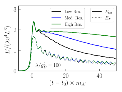
Figure 18: The total energy (solid lines) and vector field energy (dashed lines) as a function of time for $\lambda/g_{D}^{2}=100$, and three different numerical resolutions.

We perform simulations with the following parameters. We assume a translation symmetry in one direction and consider cases with $\lambda/g_{D}^{2}=100$, 200, and 400, choosing $t_{0}$ such that the average energy density reaches $\langle\rho\rangle\approx 2\lambda v^{4}$. For $\lambda/g_{D}^{2}=100$, we also vary the time of the axion instability shutoff $t_{0}$ by $\approx\pm 1.2/m_{A^{\prime}}$. Finally, we consider a fully 3D case assuming no symmetries with $\lambda/g_{D}^{2}=25$ and $L=2\pi/k_{p}$, as well as the equivalent case with a translational symmetry for comparison. For this case $dx\approx 0.12\lambda^{-1/2}v^{-1}$.

Appendix B Klein Gordon equation in a background electric and magnetic field

In this appendix, we review the solution of Klein Gordon equation in a background electric and magnetic field. We will work in the Landau gauge and comment on the differences between the electric and magnetic field. Consider the following action

$$\mathcal{S}=\int{\rm d}^{4}x\left(\left|D_{\mu}\Phi\right|^{2}-\frac{1}{4}F^{\mu\nu}F_{\mu\nu}-m^{2}\left|\Phi\right|^{2}\right),$$ (53)

where $m^{2}$ can be both positive and negative. We will consider a constant magnetic field pointing in the z-direction, and an electric field that is either parallel or perpendicular to the magnetic field. To start with, however, we consider only a background magnetic field. The correction to the scalar effective potential from a constant magnetic field is computed in Lam:1971my . The equation of motion is

$$\left[(\boldsymbol{\mathbf{p}}-e\boldsymbol{\mathbf{A}})^{2}+m^{2}\right]\Phi=(p_{0}-eA_{0})\Phi,$$ (54)

with $A_{x}=-yB_{z}$ and $A_{0}=A_{y}=A_{z}=0$. The equation of motion can be written as

$$\left[-\frac{d^{2}}{dy^{2}}+(eB_{z})^{2}(y+p_{x}/eB_{z})^{2}+p_{z}^{2}-\omega^{2}+m^{2}\right]Y[y]=0,$$ (55)

where $\Phi=Y[y]\exp[ip_{x}x+ip_{z}z-i\omega t]$. Changing variable from $y$ to $\tilde{y}$ through $\tilde{y}=|eB_{z}|^{1/2}(y+p_{x}/eB_{z})$, we can rewrite equation 55 as

$$\left[-\frac{d^{2}}{d\tilde{y}^{2}}+\tilde{y}^{2}+\frac{p_{z}^{2}-\omega^{2}+m^{2}}{eB_{z}}\right]Y[y]=0,$$ (56)

and find the solutions with Hermite polynomials $H_{n}(\tilde{y})$ as $Y(\tilde{y})=\exp^{-\tilde{y}^{2}/2}H_{n}(\tilde{y})$, and the dispersion relation is

$$\omega^{2}=p_{x}^{2}+p_{z}^{2}+m^{2}+|eB_{z}|(2n+1),\quad n=0,\,1,\,2,\ \ldots,$$ (57)

which reduces to the standard Landau level result in the non-relativistic limit. A scalar receives a positive correction to its mass squared $m_{B}^{2}=|eB_{z}|(2n+1)$ in a background magnetic field. Such a correction can help restore a broken $U(1)$ symmetry (the bare $m^{2}$ is negative) when $|eB_{z}|>|m^{2}|$.

Similarly, we can also add an electric field that is either parallel or perpendicular to the magnetic field. If the electric and magnetic field are parallel, we can choose the gauge where $A_{x}=-yB_{z}$, $A_{0}=-zE_{z}$, and $A_{y}=A_{z}=0$, which has a solution $\Phi=Y[y]Z[z]\exp[ip_{x}x-i\omega t]$ satisfying

$$\left[-\frac{d^{2}}{dy^{2}}+(eB_{z})^{2}(y+p_{x}/eB_{z})^{2}-m_{B}^{2}\right]Y[y]=0,$$

$$\left[-\frac{d^{2}}{dz^{2}}-(\omega+eE_{z}z)^{2}+m^{2}+m_{B}^{2}\right]Z[z]=0.$$ (58)

Note that the effect of the electric field and magnetic field is totally separable in this case, and as a result, the solution in a purely electric field background corresponding to solving the equations with $m_{B}=0$. Performing a similar change of variables $\tilde{z}=(eE_{z})^{1/2}(z+\omega/eE_{z})$ allows us to rewrite equation 58 as

$$\left[-\frac{d^{2}}{d\tilde{z}^{2}}-\tilde{z}^{2}+\frac{m_{B}^{2}+m^{2}}{eE_{z}}\right]Y[y]=0,$$ (59)

and find the solution as Kummer functions

$$Z(\tilde{z})=F\left[\frac{1}{4}\left(1+i\frac{m^{2}+m_{B}^{2}}{4eE_{z}}\right),\,\frac{1}{2},\,-i\tilde{z}^{2}\right]\quad\text{or}\quad F\left[\frac{1}{4}\left(1+i\frac{m^{2}+m_{B}^{2}}{4eE_{z}}\right)+\frac{1}{2},\,\frac{3}{2},\,-i\tilde{z}^{2}\right].$$ (60)

Despite the complicated appearance of the solution, the main difference between the equations of motion in 59 and 56 is the sign of the second term, which determines if the third entry of the Kummer function is real or imaginary. The solution in the electric field is not an energy eigenstate, which is expected since charged particles are generically accelerated by the electric field. Mathematically, both the first and second kind Kummer function is a viable solution to the equation of motion.

If the electric field is perpendicular to the magnetic field, we can choose the gauge where $A_{x}=-yB_{z}$, $A_{0}=-yE_{y}$ and $A_{y}=A_{z}=0$. In this case, the electric and magnetic field has effects that are not separable, and the solution is $\Phi=Y[y]\exp[ip_{x}x+ip_{z}z-i\omega t]$, with equation of motion

$$\left[-\frac{d^{2}}{dy^{2}}-e^{2}(E_{y}^{2}-B_{z}^{2})y^{2}-2ey(\omega E_{y}-p_{x}B_{z})+p_{x}^{2}+p_{z}^{2}-\omega^{2}+m^{2}\right]Y[y]=0.$$ (61)

For $E_{y}^{2}-B_{z}^{2}\neq 0$, we can define the Lorentz invariant field strength $F^{2}\equiv E_{y}^{2}-B_{z}^{2}$, perform a change of variables $\tilde{y}=(eF)^{1/2}(y-(B_{z}p_{x}-\omega E_{y})/eF^{2})$ and solve the differential equations. This change of variable reduces to the above-mentioned change of variables in the limit where $E$ or $B$ is zero. As expected, the coefficient of the $y^{2}$ term is Lorentz invariant and gauge invariant, which makes sense, since if the electric and magnetic field are perpendicular, one can always perform a Lorentz transformation to go to a frame where only one of the two fields exist. It should be noted that the above discussion only concerns time-independent and spatially uniform electric and magnetic fields. The conditions for symmetry restoration in a background field that is time dependent (radio lasers) and spatially non-uniform electric field (in particular if $\nabla\times E\neq 0$) is much more complicated, and we refer readers to tinkham2004introduction for more discussion of this.

To conclude, we showed in this appendix the gauge invariant equations of motion and eigenfunctions of scalar QED. As we demonstrated with the case including an electric field, increasing the vector potential $A^{\mu}$, which is not gauge invariant, does not necessarily contribute to a breaking or restoration of a $U(1)$ symmetry. In the background of a magnetic field, the zero mode of the scalar field gets a positive mass squared equal to $eB$, and the $U(1)$ symmetry can be restored globally when $eB>\lambda v^{2}$, in agreement with the value we have in equation 4.

Appendix C Possible resolutions for dark photon production mechanisms

Possible resolutions to the problems with the dark photon production mechanisms implied by vortex formation can be separated into two categories. The first is to add new dynamics that makes the dark photon mass different during and after inflation, or more generally, during production and today. Secondly, the dynamics studied in this paper does not apply to the case where the mass of the dark photon is introduced simply as a relevant operator that does not have a UV origin, in which case the mass of the dark photon can be considered as a parameter that breaks a shift symmetry instead of spontaneous breaking a $U(1)$ gauge symmetry. In this case, the Goldstone boson that is eaten by the photon to become the longitudinal polarization of the massive photon is not necessarily compact, and the dynamics we study in this paper does not happen. In the following, we outline two model building approaches that can resolve the issues discussed in this paper following the above-mentioned ideas.

C.1 Clockwork Mechanism

A possible resolution of both the issue of inflationary production, as well as that of a late time production mechanism, is to introduce a clockwork mechanism Gherghetta:2019coi that creates a separation between the charge of the Higgs field and a fermion field $\Psi$ that mediates the mixing between the dark photon and the standard model photon, so as to have an observable dark photon. Such models have been invoked mainly to explain a small kinetic mixing parameter assuming an $\mathcal{O}(1)$ dark gauge coupling Gherghetta:2019coi . In our case, we apply the mechanism in the opposite direction to explain the lightness of the dark photon given a large VEV. Consider the following Lagrangian

$$\mathcal{L}=\left|D_{\mu}\Phi_{i,\,i+1}\right|^{2}-\frac{\lambda}{4}\left(\left|\Phi_{i,\,i+1}\right|^{2}-v_{i,\,i+1}^{2}\right)^{2}-\frac{1}{4}F_{i}^{\mu\nu}F_{i\mu\nu}$$ (62)

where the covariant derivative $D^{\mu}\Phi_{i,\,i+1}=(\partial^{\mu}-iq_{i}g_{i}A_{i}^{\mu}+iq_{i+1}g_{i+1}A_{i+1}^{\mu})\Phi_{ij}$. The gauge couplings are chosen to be equal ($g_{i}=g_{D}$) and the scalar charges are chosen to be $(q_{i},q_{i+1})=(Q_{R},1)$ under the two consecutive gauge groups $U(1)_{i}$ and $U(1)_{i+1}$ (see figure 19). After symmetry breaking, $\langle\Phi_{i,\,i+1}\rangle=v_{i,\,i+1}$, the original $U(1)^{N}$ gauge symmetry is broken down to a single $U(1)_{D}$ by the $N-1$ Higgs fields $\Phi_{i,\,i+1}$, and the Higgs field $\Phi$ and the fermion field $\Psi$ have an effective charge $(q_{D\Phi},q_{D\Psi})=(1/Q_{R}^{N-1},1)$ under the remaining gauge group, which we identify as $U(1)_{D}$. The kinetic mixing between $U(1)_{\rm EM}$ and $U(1)_{D}$ is generated through a $\Psi$ loop, and current experimental sensitivity probes a region Baryakhtar:2017ngi ; Cervantes:2022yzp ; Chiles:2021gxk ; AxionLimits :

$$\epsilon=\frac{q_{D\Psi}q_{\Psi}eg_{D}}{16\pi^{2}}\gtrsim 10^{-16}\ ,$$ (63)

while $g_{D}q_{\Phi}\lesssim 10^{-22}$ from eq. 19. Therefore, for the parameter space of interest, we have

$$q_{D\Psi}/q_{D\Phi}\gtrsim 10^{8}.$$ (64)

Such a clockwork mechanism works because in the limit where the gauge group is $R$ instead of a $U(1)$, the Goldstone direction is no longer compact/periodic, and hence vortex production is impossible.

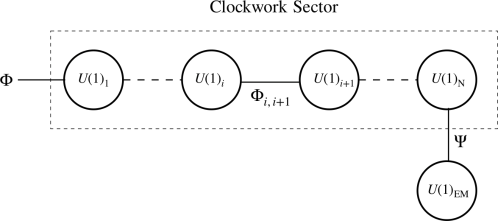
Figure 19: The clockwork model that can generate a large kinetic mixing but a tiny dark photon mass. The various VEVs of scalars $\Phi_{i,\,i+1}$ break the $U(1)^{N}$ gauge groups in the dashed box down to a single dark $U(1)_{D}$. The dark photon gets a mass from the VEV of the scalar $\Phi$, while the fermion $\Psi$ generates the kinetic mixing between $U(1)_{D}$ and $U(1)_{\rm EM}$.

However, unlike the normal clockwork models, where the VEVs of the scalar field that breaks the $U(1)^{N}$ symmetry down to the diagonal can be arbitrary, as long as they are larger than the VEV that breaks the final $U(1)$ symmetry to generate a dark photon mass, in the case of late time dark photon production mechanisms, these VEVs have to be much larger. The clockwork scalars are coupled with up to $\mathcal{O}(1)$ $U(1)_{D}$ charges and vortices of these scalars $\Phi_{i}$ are more likely to be nucleated in the background field. This is a hierarchy problem of $v_{i,\,i+1}/v\sim q_{D\Psi}/q_{D\Phi}\sim 10^{8}$.

C.2 Non-minimal coupling

Another possible resolution to the issue of vortex formation during the inflationary production of dark photons is to introduce a non-minimal coupling of the scalar field to the Ricci Scalar $R$ of the form $\xi_{\Phi}|\Phi|^{2}R$. Such a coupling can change the potential of the scalar field. In particular, it can increase the VEV beyond the Hubble scale when $\xi_{\Phi}<0$ and $|\xi_{\Phi}|\gg 1$, which can suppress vortex production. However, such a suppression goes as

$$\exp[-4\pi^{2}v^{2}/H^{2}]\sim\exp\left[-4\pi^{2}\frac{6|\xi_{\Phi}|}{\lambda}\right].$$ (65)

for $\lambda\gg 1$, up to power law corrections. This exponential suppression, however, needs to be compared to the large number of Hubble patches at the end of inflation, of order $\exp{180}$. If a significant fraction of the Hubble patches contain a vortex, these vortices can consume the energy stored in the dark photon dark matter field produced in the Hubble patches without a seed vortex and expand, converting a significant portion of the total energy density into vortices. This suggests that a large non-minimal coupling might be needed to avoid the system eventually reaching the scaling solution.

A large non-minimal coupling can help avoid vortex production, however, the coupling also changes the relation between the dark photon mass and the inflationary Hubble scale implied by the dark photon dark matter. In particular, after inflation, both the field $\Pi$ and the Higgs VEV $v$ are functions of time. The dimensionless angular variable $\Pi/v$, instead of $\Pi$, will be constant during adiabatic evolution (see the text around equation 2 for the definition). In order to not have strings form due to the Kibble mechanism, it is also required that $\Pi/v$ never exceed $2\pi$. Therefore, though a large non-minimal coupling can stop string production during inflation, it still does not help solve the issue of producing sufficient dark photon dark matter.

Appendix D Notation

Parameter (DP)	Description (DP)	Parameter (SC)	Description (SC)
$m_{A^{\prime}}=g_{D}v$	dark photon mass	$\delta=m_{A}^{-1}$	London penetration depth
$m_{\rho}=\lambda^{1/2}v$	dark Higgs mass	$\xi=m_{\rho}^{-1}$	coherence length
$\kappa=\delta/\xi$		$\kappa^{2}=\lambda/g_{D}^{2}$
$\Phi_{0}^{\prime}=2\pi/g_{D}$	flux quanta	$\Phi_{0}=\pi/e$	flux quanta
$B_{c1}^{\prime}=g_{D}v^{2}$	dark residual field	$H_{c1}=\frac{\Phi_{0}}{4\pi\delta^{2}}\log\kappa$	first critical field
$B_{c2}^{\prime}=\lambda v^{2}/g_{D}$	symmetry restoration	$H_{c2}=\frac{\Phi_{0}}{2\pi\xi^{2}}$	second critical field
$B_{\rm sh}^{\prime}=\lambda^{1/2}v^{2}$	superheating field	$H_{\rm sh}=\frac{C_{\rm sh}\Phi_{0}}{\delta\xi}$	superheating field

Table 1: A list of useful variables and terminology, their definitions in the dark photon (DP) and superconductor (SC) literature, as well as how the various variables and terminology are related/analogous to each other. A more detailed discussion can be found in tinkham2004introduction and section 2

.

References

- (1) B. Holdom, Two U(1)’s and Epsilon Charge Shifts, Phys. Lett. B166 (1986) 196.
- (2) A. Arvanitaki, S. Dimopoulos, S. Dubovsky, N. Kaloper, and J. March-Russell, String Axiverse, Phys. Rev. D 81 (2010) 123530, [arXiv:0905.4720].
- (3) M. Goodsell, J. Jaeckel, J. Redondo, and A. Ringwald, Naturally Light Hidden Photons in LARGE Volume String Compactifications, JHEP 11 (2009) 027, [arXiv:0909.0515].
- (4) M. Pospelov, A. Ritz, and M. B. Voloshin, Bosonic super-WIMPs as keV-scale dark matter, Phys. Rev. D 78 (2008) 115012, [arXiv:0807.3279].
- (5) R. Essig, J. Mardon, and T. Volansky, Direct Detection of Sub-GeV Dark Matter, Phys. Rev. D 85 (2012) 076007, [arXiv:1108.5383].
- (6) H. An, M. Pospelov, and J. Pradler, New stellar constraints on dark photons, Phys. Lett. B 725 (2013) 190–195, [arXiv:1302.3884].
- (7) E. Hardy and R. Lasenby, Stellar cooling bounds on new light particles: plasma mixing effects, JHEP 02 (2017) 033, [arXiv:1611.05852].
- (8) R. Lasenby, Long range dark matter self-interactions and plasma instabilities, JCAP 11 (2020) 034, [arXiv:2007.00667].
- (9) J. Jaeckel, J. Redondo, and A. Ringwald, Signatures of a hidden cosmic microwave background, Phys. Rev. Lett. 101 (2008) 131801, [arXiv:0804.4157].
- (10) A. Caputo, H. Liu, S. Mishra-Sharma, and J. T. Ruderman, Dark Photon Oscillations in Our Inhomogeneous Universe, Phys. Rev. Lett. 125 (2020), no. 22 221303, [arXiv:2002.05165].
- (11) M. Baryakhtar, R. Lasenby, and M. Teo, Black Hole Superradiance Signatures of Ultralight Vectors, Phys. Rev. D 96 (2017), no. 3 035019, [arXiv:1704.05081].
- (12) P. W. Graham, J. Mardon, and S. Rajendran, Vector Dark Matter from Inflationary Fluctuations, Phys. Rev. D93 (2016), no. 10 103520, [arXiv:1504.02102].
- (13) A. E. Nelson and J. Scholtz, Dark Light, Dark Matter and the Misalignment Mechanism, Phys. Rev. D 84 (2011) 103501, [arXiv:1105.2812].
- (14) P. Agrawal, N. Kitajima, M. Reece, T. Sekiguchi, and F. Takahashi, Relic Abundance of Dark Photon Dark Matter, Phys. Lett. B 801 (2020) 135136, [arXiv:1810.07188].
- (15) S. Chaudhuri, P. W. Graham, K. Irwin, J. Mardon, S. Rajendran, and Y. Zhao, Radio for hidden-photon dark matter detection, Phys. Rev. D92 (2015), no. 7 075012, [arXiv:1411.7382].
- (16) M. Baryakhtar, J. Huang, and R. Lasenby, Axion and hidden photon dark matter detection with multilayer optical haloscopes, Phys. Rev. D 98 (Aug, 2018) 035006.
- (17) SuperCDMS Collaboration Collaboration, T. Aralis, T. Aramaki, I. J. Arnquist, E. Azadbakht, W. Baker, S. Banik, D. Barker, C. Bathurst, D. A. Bauer, L. V. S. Bezerra, R. Bhattacharyya, T. Binder, M. A. Bowles, P. L. Brink, R. Bunker, B. Cabrera, R. Calkins, R. A. Cameron, C. Cartaro, D. G. Cerdeño, Y.-Y. Chang, J. Cooley, H. Coombes, J. Corbett, B. Cornell, P. Cushman, F. De Brienne, M. L. di Vacri, M. D. Diamond, E. Fascione, E. Figueroa-Feliciano, C. W. Fink, K. Fouts, M. Fritts, G. Gerbier, R. Germond, M. Ghaith, S. R. Golwala, H. R. Harris, N. Herbert, B. A. Hines, M. I. Hollister, Z. Hong, E. W. Hoppe, L. Hsu, M. E. Huber, V. Iyer, D. Jardin, A. Jastram, M. H. Kelsey, A. Kennedy, A. Kubik, N. A. Kurinsky, R. E. Lawrence, A. Li, B. Loer, E. Lopez Asamar, P. Lukens, D. MacDonell, D. B. MacFarlane, R. Mahapatra, V. Mandic, N. Mast, E. M. Michaud, E. Michielin, N. Mirabolfathi, B. Mohanty, J. D. Morales Mendoza, S. Nagorny, J. Nelson, H. Neog, J. L. Orrell, S. M. Oser, W. A. Page, P. Pakarha, R. Partridge, R. Podviianiuk, F. Ponce, S. Poudel, M. Pyle, W. Rau, R. Ren, T. Reynolds, A. Roberts, A. E. Robinson, H. E. Rogers, T. Saab, B. Sadoulet, J. Sander, R. W. Schnee, S. Scorza, K. Senapati, B. Serfass, D. J. Sincavage, C. Stanford, M. Stein, J. Street, D. Toback, R. Underwood, S. Verma, A. N. Villano, B. von Krosigk, S. L. Watkins, L. Wills, J. S. Wilson, M. J. Wilson, J. Winchell, D. H. Wright, S. Yellin, B. A. Young, T. C. Yu, E. Zhang, X. Zhao, and L. Zheng, Constraints on dark photons and axionlike particles from the supercdms soudan experiment, Phys. Rev. D 101 (Mar, 2020) 052008.
- (18) The FUNK Experiment Collaboration, A. Andrianavalomahefa, C. M. Schäfer, D. Veberič, R. Engel, T. Schwetz, H.-J. Mathes, K. Daumiller, M. Roth, D. Schmidt, R. Ulrich, B. Döbrich, J. Jaeckel, M. Kowalski, A. Lindner, and J. Redondo, Limits from the funk experiment on the mixing strength of hidden-photon dark matter in the visible and near-ultraviolet wavelength range, Phys. Rev. D 102 (Aug, 2020) 042001.
- (19) SENSEI Collaboration Collaboration, L. Barak, I. M. Bloch, M. Cababie, G. Cancelo, L. Chaplinsky, F. Chierchie, M. Crisler, A. Drlica-Wagner, R. Essig, J. Estrada, E. Etzion, G. F. Moroni, D. Gift, S. Munagavalasa, A. Orly, D. Rodrigues, A. Singal, M. S. Haro, L. Stefanazzi, J. Tiffenberg, S. Uemura, T. Volansky, and T.-T. Yu, Sensei: Direct-detection results on sub-gev dark matter from a new skipper ccd, Phys. Rev. Lett. 125 (Oct, 2020) 171802.
- (20) J. Chiles et al., First Constraints on Dark Photon Dark Matter with Superconducting Nanowire Detectors in an Optical Haloscope, arXiv:2110.01582.
- (21) R. Cervantes et al., Search for 70 V Dark Photon Dark Matter with a Dielectrically-Loaded Multi-Wavelength Microwave Cavity, arXiv:2204.03818.
- (22) L. P. Gor’kov, Microscopic derivation of the ginzburg–landau equations in the theory of superconductivity, Sov. Phys. - JETP (Engl. Transl.); (United States) 9:6 (1, 1959).
- (23) Die Wechselwirkungskräfte in der Elektrodynamik und in der Feldtheorie der Kernkräfte (Teil II und III) [40], in E.C.G. Stueckelberg, An Unconventional Figure of Twentieth Century Physics, p. 273. 2009.
- (24) L. Lam, Motion in electric and magnetic fields. 1. klein-gordon particles, J. Math. Phys. 12 (1971) 299–303.
- (25) M. Tinkham, Introduction to Superconductivity. Dover Publications, 2 ed., June, 2004.
- (26) Y. Nambu, Lectures on the Copenhagen Summer Symposium (1970), unpublished, .
- (27) A. A. Abrikosov, On the Magnetic properties of superconductors of the second group, Sov. Phys. JETP 5 (1957) 1174–1182.
- (28) H. B. Nielsen and P. Olesen, Vortex Line Models for Dual Strings, Nucl. Phys. B 61 (1973) 45–61.
- (29) R. T. Co, A. Pierce, Z. Zhang, and Y. Zhao, Dark Photon Dark Matter Produced by Axion Oscillations, Phys. Rev. D 99 (2019), no. 7 075002, [arXiv:1810.07196].
- (30) J. A. Dror, K. Harigaya, and V. Narayan, Parametric Resonance Production of Ultralight Vector Dark Matter, Phys. Rev. D 99 (2019), no. 3 035036, [arXiv:1810.07195].
- (31) M. Bastero-Gil, J. Santiago, L. Ubaldi, and R. Vega-Morales, Vector dark matter production at the end of inflation, JCAP 04 (2019) 015, [arXiv:1810.07208].
- (32) H. Fukuda and K. Nakayama, Aspects of Nonlinear Effect on Black Hole Superradiance, JHEP 01 (2020) 128, [arXiv:1910.06308].
- (33) W. E. East, Vortex String Formation in Black Hole Superradiance of a Dark Photon with the Higgs Mechanism, arXiv:2205.03417.
- (34) P. Pani, V. Cardoso, L. Gualtieri, E. Berti, and A. Ishibashi, Black hole bombs and photon mass bounds, Phys. Rev. Lett. 109 (2012) 131102, [arXiv:1209.0465].
- (35) S. Endlich and R. Penco, A Modern Approach to Superradiance, JHEP 05 (2017) 052, [arXiv:1609.06723].
- (36) W. E. East, Superradiant instability of massive vector fields around spinning black holes in the relativistic regime, Phys. Rev. D96 (2017), no. 2 024004, [arXiv:1705.01544].
- (37) V. Cardoso, O. J. C. Dias, G. S. Hartnett, M. Middleton, P. Pani, and J. E. Santos, Constraining the mass of dark photons and axion-like particles through black-hole superradiance, JCAP 1803 (2018), no. 03 043, [arXiv:1801.01420].
- (38) R. Brito, V. Cardoso, and P. Pani, Black holes as particle detectors: evolution of superradiant instabilities, Classical and Quantum Gravity 32 (2015), no. 13 134001.
- (39) W. E. East and F. Pretorius, Superradiant Instability and Backreaction of Massive Vector Fields around Kerr Black Holes, Phys. Rev. Lett. 119 (2017), no. 4 041101, [arXiv:1704.04791].
- (40) W. E. East, Massive Boson Superradiant Instability of Black Holes: Nonlinear Growth, Saturation, and Gravitational Radiation, Phys. Rev. Lett. 121 (2018), no. 13 131104, [arXiv:1807.00043].
- (41) A. Arvanitaki and S. Dubovsky, Exploring the String Axiverse with Precision Black Hole Physics, Phys. Rev. D83 (2011) 044026, [arXiv:1004.3558].
- (42) A. A. Varlamov, A. Galda, and A. Glatz, Fluctuation spectroscopy: From rayleigh-jeans waves to abrikosov vortex clusters, Rev. Mod. Phys. 90 (Mar, 2018) 015009.
- (43) V. P. Galaiko, Formation of vortex nuclei in superconductors of the second kind, Journal of Experimental and Theoretical Physics (1966).
- (44) V. P. Galaiko, Stability limits of the superconducting state in a magnetic field for superconductors of the second kind, Zhurnal Eksperimental’noi i Teoreticheskoi Fiziki (U.S.S.R.) For English translation see Sov. Phys. - JETP (Engl. Transl.) Vol: 50 (3, 1966).
- (45) D. B. Liarte, M. K. Transtrum, and J. P. Sethna, Ginzburg-landau theory of the superheating field anisotropy of layered superconductors, Physical Review B 94 (2016), no. 14 144504.
- (46) L. Kramer, Stability limits of the meissner state and the mechanism of spontaneous vortex nucleation in superconductors, Phys. Rev. 170 (Jun, 1968) 475–480.
- (47) A. D. Hernández and D. Domínguez, Surface barrier in mesoscopic type-i and type-ii superconductors, Phys. Rev. B 65 (Apr, 2002) 144529.
- (48) M. K. Transtrum, G. Catelani, and J. P. Sethna, Superheating field of superconductors within ginzburg-landau theory, Phys. Rev. B 83 (Mar, 2011) 094505.
- (49) E. Zeldov, D. Majer, M. Konczykowski, V. B. Geshkenbein, V. M. Vinokur, and H. Shtrikman, Thermodynamic observation of first-order vortex-lattice melting transition in bi2sr2cacu2o8, Nature 375 (1995), no. 6530 373–376.
- (50) M. James, D. A. Suchla, J. Dunkel, and M. Wilczek, Emergence and melting of active vortex crystals, Nature communications 12 (2021), no. 1 1–11.
- (51) F. Liu, M. Mondello, and N. Goldenfeld, Kinetics of the superconducting transition, Physical review letters 66 (1991), no. 23 3071.
- (52) K. Binder, Time-dependent ginzburg-landau theory of nonequilibrium relaxation, Phys. Rev. B 8 (Oct, 1973) 3423–3438.
- (53) R. Basu, A. H. Guth, and A. Vilenkin, Quantum creation of topological defects during inflation, Phys. Rev. D 44 (Jul, 1991) 340–351.
- (54) T. Gherghetta, J. Kersten, K. Olive, and M. Pospelov, Evaluating the price of tiny kinetic mixing, Phys. Rev. D 100 (2019), no. 9 095001, [arXiv:1909.00696].
- (55) A. Arvanitaki, S. Dimopoulos, M. Galanis, D. Racco, O. Simon, and J. O. Thompson, Dark QED from inflation, JHEP 11 (2021) 106, [arXiv:2108.04823].
- (56) N. Arkani-Hamed, L. Motl, A. Nicolis, and C. Vafa, The String landscape, black holes and gravity as the weakest force, JHEP 06 (2007) 060, [hep-th/0601001].
- (57) M. Reece, Photon Masses in the Landscape and the Swampland, JHEP 07 (2019) 181, [arXiv:1808.09966].
- (58) M. Buschmann, J. W. Foster, A. Hook, A. Peterson, D. E. Willcox, W. Zhang, and B. R. Safdi, Dark matter from axion strings with adaptive mesh refinement, Nature Commun. 13 (2022), no. 1 1049, [arXiv:2108.05368].
- (59) M. E. Peskin, Mandelstam ’t Hooft Duality in Abelian Lattice Models, Annals Phys. 113 (1978) 122.
- (60) J. Polchinski and J. V. Rocha, Analytic study of small scale structure on cosmic strings, Phys. Rev. D 74 (2006) 083504, [hep-ph/0606205].
- (61) C. Bachas and M. Porrati, Pair creation of open strings in an electric field, Phys. Lett. B 296 (1992) 77–84, [hep-th/9209032].
- (62) R. O. Ramos, J. F. Medeiros Neto, D. G. Barci, and C. A. Linhares, Abelian Higgs model effective potential in the presence of vortices, Phys. Rev. D 72 (2005) 103524, [hep-th/0506052].
- (63) M. B. Hindmarsh and T. W. B. Kibble, Cosmic strings, Rept. Prog. Phys. 58 (1995) 477–562, [hep-ph/9411342].
- (64) V. P. Frolov, S. Hendy, and A. L. Larsen, How to create a 2-D black hole, Phys. Rev. D 54 (1996) 5093–5102, [hep-th/9510231].
- (65) S. Kinoshita, T. Igata, and K. Tanabe, Energy extraction from Kerr black holes by rigidly rotating strings, Phys. Rev. D 94 (2016), no. 12 124039, [arXiv:1610.08006].
- (66) T. Igata, H. Ishihara, M. Tsuchiya, and C.-M. Yoo, Rigidly Rotating String Sticking in a Kerr Black Hole, Phys. Rev. D 98 (2018), no. 6 064021, [arXiv:1806.09837].
- (67) H. Xing, Y. Levin, A. Gruzinov, and A. Vilenkin, Spinning black holes as cosmic string factories, Phys. Rev. D 103 (2021), no. 8 083019, [arXiv:2011.00654].
- (68) T. Kibble, Some implications of a cosmological phase transition, Physics Reports 67 (1980), no. 1 183–199.
- (69) W. H. Zurek, Cosmological experiments in superfluid helium?, Nature 317 (1985), no. 6037 505–508.
- (70) T. W. B. Kibble and G. E. Volovik, On phase ordering behind the propagating front of a second order transition, JETP Lett. 65 (1997) 102–107, [cond-mat/9612075].
- (71) A. J. Long and L.-T. Wang, Dark Photon Dark Matter from a Network of Cosmic Strings, Phys. Rev. D 99 (2019), no. 6 063529, [arXiv:1901.03312].
- (72) Planck Collaboration, N. Aghanim et al., Planck 2018 results. VI. Cosmological parameters, Astron. Astrophys. 641 (2020) A6, [arXiv:1807.06209]. [Erratum: Astron.Astrophys. 652, C4 (2021)].
- (73) C. J. Moore, R. H. Cole, and C. P. L. Berry, Gravitational-wave sensitivity curves, Class. Quant. Grav. 32 (2015), no. 1 015014, [arXiv:1408.0740].
- (74) C. O’Hare, “cajohare/axionlimits: Axionlimits.” https://cajohare.github.io/AxionLimits/, July, 2020.
- (75) J. C. Allred, R. N. Lyman, T. W. Kornack, and M. V. Romalis, High-sensitivity atomic magnetometer unaffected by spin-exchange relaxation, Phys. Rev. Lett. 89 (Sep, 2002) 130801.
- (76) T. Charnock, A. Avgoustidis, E. J. Copeland, and A. Moss, CMB constraints on cosmic strings and superstrings, Phys. Rev. D 93 (2016), no. 12 123503, [arXiv:1603.01275].
- (77) L. Dai and J. Miralda-Escudé, Gravitational Lensing Signatures of Axion Dark Matter Minihalos in Highly Magnified Stars, Astron. J. 159 (2020), no. 2 49, [arXiv:1908.01773].
- (78) K. Van Tilburg, A.-M. Taki, and N. Weiner, Halometry from Astrometry, JCAP 07 (2018) 041, [arXiv:1804.01991].
- (79) E. Adelberger, G. Dvali, and A. Gruzinov, Photon mass bound destroyed by vortices, Phys. Rev. Lett. 98 (2007) 010402, [hep-ph/0306245].
- (80) L.-T. Wang and Z.-Z. Xianyu, Gauge boson signals at the cosmological collider, Journal of High Energy Physics 2020 (2020), no. 11 1–27.
- (81) M. Zilhão, H. Witek, and V. Cardoso, Nonlinear interactions between black holes and Proca fields, Class. Quant. Grav. 32 (2015) 234003, [arXiv:1505.00797].
- (82) T. Helfer, J. C. Aurrekoetxea, and E. A. Lim, Cosmic String Loop Collapse in Full General Relativity, Phys. Rev. D 99 (2019), no. 10 104028, [arXiv:1808.06678].