Geometry Interaction Knowledge Graph Embeddings

Abstract

Knowledge graph (KG) embeddings have shown great power in learning representations of entities and relations for link prediction tasks. Previous work usually embeds KGs into a single geometric space such as Euclidean space (zero curved), hyperbolic space (negatively curved) or hyperspherical space (positively curved) to maintain their specific geometric structures (e.g., chain, hierarchy and ring structures). However, the topological structure of KGs appears to be complicated, since it may contain multiple types of geometric structures simultaneously. Therefore, embedding KGs in a single space, no matter the Euclidean space, hyperbolic space or hyperspheric space, cannot capture the complex structures of KGs accurately. To overcome this challenge, we propose Geometry Interaction knowledge graph Embeddings (GIE), which learns spatial structures interactively between the Euclidean, hyperbolic and hyperspherical spaces. Theoretically, our proposed GIE can capture a richer set of relational information, model key inference patterns, and enable expressive semantic matching across entities. Experimental results on three well-established knowledge graph completion benchmarks show that our GIE achieves the state-of-the-art performance with fewer parameters.

Introduction

Knowledge Graphs (KGs) attract more and more attentions in the past years, which play an important role in many semantic applications (e.g., question answering (Diefenbach, Singh, and Maret 2018; Keizer et al. 2017), semantic search (Berant et al. 2013; Berant and Liang 2014), recommender systems (Gong et al. 2020; Guo et al. 2020), and dialogue generation (Keizer et al. 2017; He et al. 2017)). KGs can not only represent vast amounts of information available in the world, but also enable powerful relational reasoning. However, real-world KGs are usually incomplete, which restricts the development of downstream tasks above. To address such an issue, Knowledge Graph Embedding (KGE) emerges as an effective solution to predict missing links by the low-dimensional representations of entities and relations.

In the past decades, researchers propose various KGE methods which achieve great success. As a branch of KGE methods, learning in the Euclidean space $\mathbb{E}$ and ComplEx space $\mathbb{C}$ is highly effective, which has been demonstrated by methods such as DistMult (Yang et al. 2015), ComplEx (Trouillon et al. 2016) and TuckER (Balažević, Allen, and Hospedales 2019) (i.e., bilinear models). These methods can infer new relational triplets and capture chain structure with the scoring function based on the intuitive Euclidean distance. However, learning embeddings in Euclidean space are weak to capture complex structures (e.g., hierarchy and ring structures) (Balazevic, Allen, and Hospedales 2019b).

As another branch of KGE methods, learning KG embeddings in the non-Euclidean space (e.g., hyperspheric space $\mathbb{S}$ and hyperbolic space $\mathbb{H}$) has received wide attention in recent years. Drawing on the geometric properties of the sphere, ManifoldE (Xiao, Huang, and Zhu 2016a) embeds entities into the manifold-based space such as hypersphere space, which is beneficial to improve the precision of knowledge embedding and model the ring structure. Due to the capability of hyperbolic geometry in modeling hierarchical structure, methods such as MuRP (Balazevic, Allen, and Hospedales 2019b) and RotH (Chami et al. 2020) can outperform the methods based on Euclidean space and Complex space in knowledge graphs of hierarchical structures. However, note that most knowledge graphs embrace complicated structures as shown in Figure 1, it implies that these methods perform a bit poorly when modeling the knowledge graph with hybrid structures (Balazevic, Allen, and Hospedales 2019b) (e.g., ring, hierarchy and chain structures). Recently, (Wang et al. 2021) develops a mixed-curvature multi-relational graph neural network for knowledge graph completion, which is constructed by a Riemannian product manifold between different spaces. However, it does not delve into the interaction of the various spaces and the heterogeneity of different spaces will limit its pattern reasoning ability between spaces.

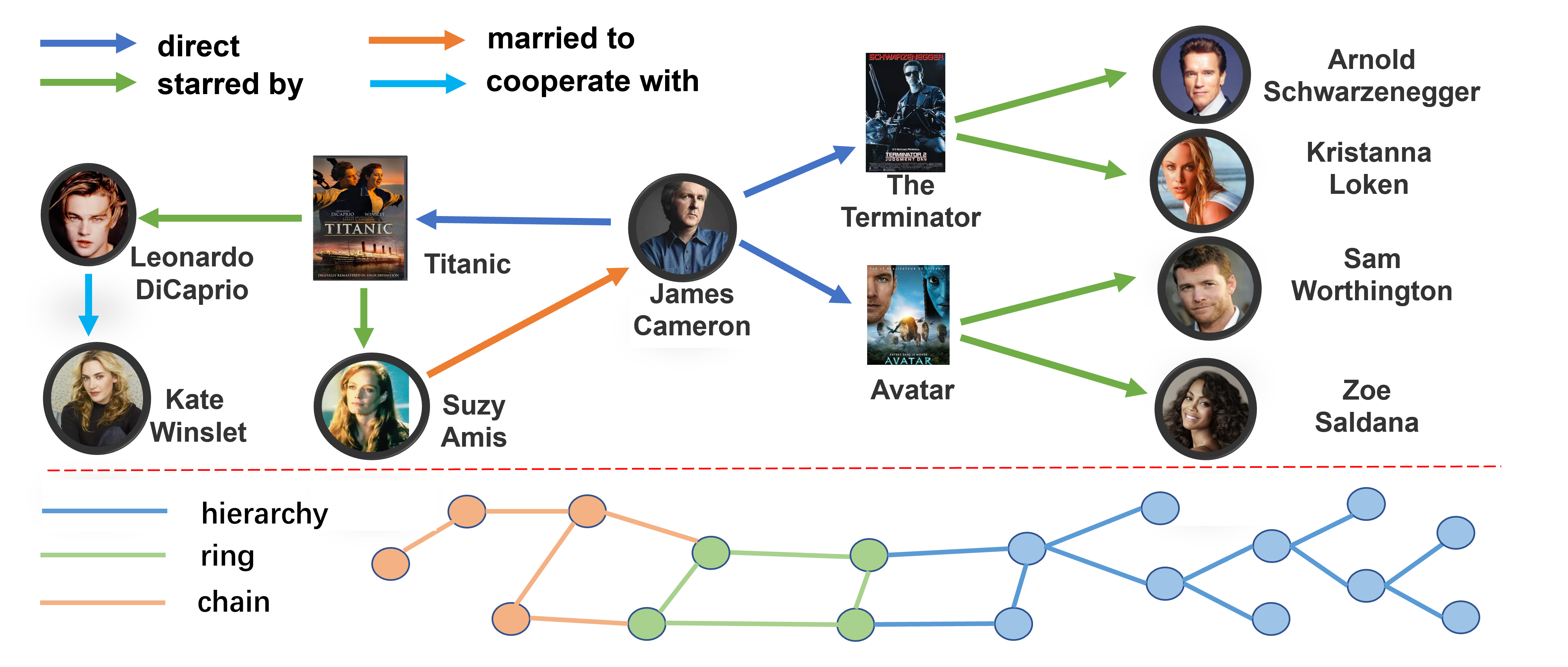
Figure 1: An illustration of the structure in knowledge graphs. The first part is a knowledge graph about the film and characters directed by James Cameron. The second part is the different spatial structure formed by different types of data such as hierarchical structure, ring structure and chain structure. Orange entities of the KG show the chain structure which can be easily modeled in an Euclidean space; green entities of the KG present ring structure which can be depicted in a hypersphere space; blue entities of the KG exhibit hierarchical structures which can be intuitively captured in a hyperbolic space.

From the analysis above, we can see learning knowledge graph embeddings without geometry interaction will inevitably result in sub-optimal results. The reason lies in that it cannot accurately capture the complex structural features of the entity location space, and the transfer of inference rules in different spaces will be affected or even invalid. Inspired by this, to capture a richer set of structural information and model key inference patterns for KG with complex structures, we attempt to embed the knowledge graph into Euclidean, hyperbolic and hyperspherical spaces jointly by geometry interaction, hoping that it can integrate the reasoning ability in different spaces.

In this paper, we take a step beyond the previous work, and propose a novel method called Geometry Interaction Knowledge Graph Embeddings (GIE). GIE can not only exploit hyperbolic, hyperspherical and Euclidean geometries simultaneously to learn the reliable structure in knowledge graphs, but also model inference rules. Specifically, we model the relations by rich geometric transformations based on special orthogonal group and special Euclidean group to utilize key inference patterns, enabling rich and expressive semantic matching between entities. Next, to approximate the complex structure guided by heterogeneous spaces, we exploit a novel geometry interaction mechanism, which is designed to capture the geometric message for complex structures in KGs. In this way, GIE can adaptively form the reliable spatial structure for knowledge graph embeddings via integrating the interactive geometric message. Moreover, experiments demonstrate that GIE can significantly outperform the state-of-the-art methods.

Our contributions are summarized as follows: 1) To the best of our knowledge, we are the first to exploit knowledge graph embeddings with geometry interaction, which adaptively learns reliable spatial structures and is equipped with the ability to transmit inference rules in complex structure of KGs. 2) We present a novel method called Geometry Interaction Knowledge Graph Embeddings (GIE), which embraces rich and expressive semantic matching between entities and satisfies the key of relational representation learning. (i.e., modeling symmetry, anti-symmetry, inversion, composition, hierarchy, intersection and mutual exclusion patterns). 3) Our model requires fewer parameters and saves about $40\%$ parameters than SOTA models, while achieving the state-of-the-art performance on three well-established knowledge graph completion benchmarks (WN18RR, FB15K237 and YAGO3-10).

Related Work

The key issue of knowledge graph embeddings is to learn low-dimensional distributed embedding of entities and relations. Previous work has proposed many KGE methods based on geometric properties of different embedding spaces. These methods mainly use Euclidean space (e.g., the vector space, matrix space and tensor space), while some methods are based on other kinds of spaces such as complex space and hyperbolic space. Moreover, there are some methods based on deep neural networks utilized as well.

Euclidean embeddings. In recent years, researchers have conducted a lot of research based on Euclidean embeddings for KG representation learning. These methods include translation approaches popularized by TransE (Bordes et al. 2013), which models the relation as the translation between head and tail entities, i.e., $head\ entity+relation\approx tail\ entity$. Then there are many variations based on TransE. TransH (Wang et al. 2014), TransR (Lin et al. 2015), TransD (Ji et al. 2015) use different projection vectors for entities and relations, separately. TorusE (Ebisu and Ichise 2018) adopts distance function in a compact Lie group to avoid forcing embeddings to be on a sphere. TransG (Xiao, Huang, and Zhu 2016b) and KG2E (He et al. 2015) further inject probabilistic principles into this framework by considering Bayesian nonparametric Gaussian mixture model and show better accuracy and scalability. And there are also tensor factorization methods such as RRESCAL (Nickel, Tresp, and Kriegel 2011), DistMult (Yang et al. 2015). These methods are very simple and intuitive, but they cannot model the key logical properties (e.g., translations cannot model symmetry).

Complex embeddings. Instead of using a real-valued embedding, learning KG embeddings in the complex space has attracted attention. Some bilinear models such as ComplEx (Trouillon et al. 2016) and HolE (Nickel, Rosasco, and Poggio 2016) measure plausibility by matching latent semantics of entities and relations. Then, RotatE (Sun et al. 2019) models the relation as the rotation in two-dimensional space, thus realizing modeling symmetry/antisymmetry, inversion and composition patterns. Inspired by RotatE, OTE (Tang et al. 2020) extends the rotation from 2D to high-dimensional space by relational transformation. Moreover, QuatE (Zhang et al. 2019) extends the complex space into the quaternion space with two rotating surfaces to enable rich semantic matching. Following this, (Cao et al. 2021) extends the embedding space to the dual quaternion space, which models the interaction of relations and entities by dual quaternion multiplication. However, complex space is essentially flat with Euclidean space since their curvatures of the space are zero. Therefore, for the KGs with the hierarchical structure, these methods often suffer from large space occupation and distortion embeddings.

Non-Euclidean embeddings. Noting the limitations of Euclidean space, ManifoldE (Xiao, Huang, and Zhu 2016a) expands pointwise modeling in the translation based principle to manifoldwise space (e.g., hypersphere space), which benefits for modeling ring structures. To capture the hierarchical structure in the knowledge graph, MuRP (Balazevic, Allen, and Hospedales 2019b) learns KG embeddings in hyperbolic space in order to target hierarchical data. (Gu et al. 2019b) proposes learning embeddings in a product manifold with a heuristic to estimate the sectional curvature of graph data. However, it ignores the interaction of the embedded spaces, which will affect the learning of spatial structure. Then ROTH (Chami et al. 2020) introduces the hyperbolic geometry on the basis of the rotation, which can achieve low-dimensional knowledge graph embeddings. However, for non-hierarchical data, their performance will be limited.

Deep neural networks. Neural network approaches such as (Jin et al. 2021b), (Yu et al. 2021),(Nathani et al. 2019) and (Jin et al. 2021a) play important roles in graph learning. Some deep neural networks have also been adopted for the KGE problem, e.g., Neural Tensor Network (Socher et al. 2013) and ER-MLP (Dong et al. 2014) are two representative neural network based methodologies. Moreover, there are some models using neural networks to produce KGE with remarkable effects. For instance, R-GCN (Schlichtkrull et al. 2018), ConvE (Dettmers et al. 2017), ConvKB (Nguyen et al. 2018), A2N (Bansal et al. 2019) and HypER (Balazevic, Allen, and Hospedales 2019a). Recently, M²GNN (Wang et al. 2021) is proposed, which is a generic graph neural network framework to embed multi-relational KG data for knowledge graph embeddings. A downside of these methods is that most of them are not interpretable.

Background and Preliminaries

Multi-relational link prediction. The multi-relational link prediction is an important task for knowledge graphs. Generally, given a set $\mathcal{E}$ of entities and a set $\mathcal{R}$ of relations, a knowledge graph $\mathcal{G}\subseteq\mathcal{E}\times\mathcal{R}\times\mathcal{E}$ is a set of subject-predicate-object triples. Noticing that the real-world knowledge graphs are often incomplete, the goal of multi-relational link prediction is to complete the KG, i.e., to predict true but unobserved triples based on the information in $\mathcal{G}$ with a score function. Typically, the score function is learned with the formula as $\phi:\mathcal{E}\times\mathcal{R}\times\mathcal{E}\rightarrow\mathbb{R}$, that assigns a score $s=\phi(\bm{h},\bm{r},\bm{t})$ to each triplet, indicating the strength of prediction that a particular triplet corresponds to a true fact. Followed closely, a non-linearity, such as the logistic or sigmoid function, is often used to convert the score to a predicted probability $p=\sigma(s)\in[0,1]$ of the triplet being true.

Non-Euclidean Geometry. Most of the manifolds in geometric space can be regarded as Riemannian manifolds $(\mathcal{M},g)$ of dimension $n$, which define the internal product operation in the tangent space $g_{\bm{x}}$ for each point $\bm{x}\in\mathcal{M}$: $\mathcal{T}_{\bm{x}}\mathcal{M}\times\mathcal{T}_{\bm{x}}\mathcal{M}\rightarrow\mathbb{R}$. The tangent space $\mathcal{T}_{\bm{x}}\mathcal{M}$ of dimension $n$ contains all possible directions of the path in non-Euclidean space leaving from $\bm{x}$. Specifically, denote $g^{E}=\bm{I}_{n}$ as the Euclidean metric tensor and $c$ as the curvature of the space, then we can use the manifold $\mathbb{M}_{c}^{n}=\left\{\boldsymbol{x}\in\mathbb{R}^{n}:c\|\boldsymbol{x}\|<1\right\}$ to define non-Euclidean space $(\mathbb{M}_{c}^{n},g^{c})$, where the following Riemannian metric $g_{\bm{x}}^{c}=\lambda_{\bm{x}}^{2}g^{E}$ and $\lambda_{\bm{x}}=\frac{2}{1-c||\bm{x}||^{2}}$.

Note that the curvature $c$ is positive for hyperspherical space $\mathbb{S}$, negative for hyperbolic space $\mathbb{H}$, and zero for Euclidean space $\mathbb{E}$. Poincar$\acute{\text{e}}$ ball is a popular adopted model in representation learning, which is commonly used in hyperbolic space and has basic mathematical operations (e.g., addition, multiplication). Moreover, it provides closed-form expressions for many basic objects such as distance and angle (Ganea, Bécigneul, and Hofmann 2018). The principled generalizations of basic operations in hyperspherical space are similar to operations in hyperbolic space, except that the curvature $c>0$. Therefore, here we only introduce the operation of hyperbolic space, the operation of hyperspherical space can be obtained by analogy.

For each point $\bm{x}$ in the hyperbolic space, we have a tangent space $\mathcal{T}_{\bm{x}}\mathbb{H}_{c}^{n}$. We can use the exponential map $\exp^{c}_{\bm{x}}:\mathcal{T}_{\bm{x}}\mathbb{H}_{c}^{n}\rightarrow\mathbb{H}_{c}^{n}$ and the logarithmic map $\log_{\bm{x}}^{c}:\mathbb{H}_{c}^{n}\rightarrow\mathcal{T}_{\bm{x}}\mathbb{H}_{c}^{n}$ to establish the connection between the hyperbolic space and tangent space as follows:

$$\exp_{\boldsymbol{x}}^{c}(\boldsymbol{v})=\boldsymbol{x}\oplus_{c}\left(\tanh\left(\sqrt{c}\frac{\lambda_{\boldsymbol{x}}\|\boldsymbol{v}\|}{2}\right)\frac{\boldsymbol{v}}{\sqrt{c}\|\boldsymbol{v}\|}\right),$$ (1)

$$\log_{\boldsymbol{x}}^{c}(\boldsymbol{y})=\frac{2}{\sqrt{c}\lambda_{\boldsymbol{x}}}\tanh^{-1}\left(\sqrt{c}\left\|-\boldsymbol{x}\oplus_{c}\boldsymbol{y}\right\|\right)\frac{-\boldsymbol{x}\oplus_{c}\boldsymbol{y}}{\left\|-\boldsymbol{x}\oplus_{c}\boldsymbol{y}\right\|},$$

where $\bm{x},\bm{y}\in\mathbb{H}_{c}^{n}$, $\bm{v}\in\mathcal{T}_{\bm{x}}\mathbb{H}_{c}^{n}$, $||\cdot||$ denotes the Euclidean norm and $\oplus_{c}$ represents M$\ddot{o}$bius addition:

$$\boldsymbol{x}\oplus_{c}\boldsymbol{y}=\frac{\left(1+2c\langle\boldsymbol{x},\boldsymbol{y}\rangle+c\|\boldsymbol{y}\|^{2}\right)\boldsymbol{x}+\left(1-c\|\boldsymbol{x}\|^{2}\right)\boldsymbol{y}}{1+2c\langle\boldsymbol{x},\boldsymbol{y}\rangle+c^{2}\|\boldsymbol{x}\|^{2}\|\boldsymbol{y}\|^{2}}.$$ (2)

The distance between two points $\bm{x},\bm{y}\in\mathbb{H}^{d}_{c}$ is measured along a geodesic (i.e., shortest path between the points) as follows:

$$d_{c}(\mathbf{x},\mathbf{y})=\frac{2}{\sqrt{c}}\tanh^{-1}\left(\sqrt{c}\left\|-\mathbf{x}\oplus_{c}\mathbf{y}\right\|\right).$$ (3)

The M$\ddot{o}$bius substraction is then defined by the use of the following notation: $\bm{x}\ominus_{c}\bm{y}=\bm{x}\oplus_{c}(-\bm{y})$. Similar to the scalar multiplication and matrix multiplication in Euclidean space, the multiplication in hyperbolic space can be defined by M$\ddot{o}$bius scalar multiplication and M$\ddot{o}$bius matrix multiplication between vectors $\bm{x}\in\mathbb{H}_{c}^{n}\{\bm{0}\}$:

$$\bm{r}\otimes_{c}\boldsymbol{x} =\frac{1}{\sqrt{c}}\tanh\left(r\tanh^{-1}(\sqrt{c}\|\boldsymbol{x}\|)\right)\frac{\boldsymbol{x}}{\|\boldsymbol{x}\|},$$ (4)

$$\bm{M}\otimes_{c}\boldsymbol{x} =(\frac{1}{\sqrt{c}})\tanh\left(\frac{\|\bm{M}\boldsymbol{x}\|}{\|\boldsymbol{x}\|}\tanh^{-1}(\sqrt{c}\|\boldsymbol{x}\|)\right)\frac{\bm{M}\boldsymbol{x}}{\|\bm{M}\boldsymbol{x}\|},$$

where $\bm{r}\in\mathbb{R}$ and $\bm{M}\in\mathbb{R}^{m\times n}$.

Methodology

Geometry Interaction Knowledge Graph Embeddings (GIE)

Problem Definition.

Given a knowledge graph $\mathcal{G}$, practically, it is usually incomplete, then the link prediction approaches are used to predict new links and complete the knowledge graph. Specifically, we learn the embeddings of relations and entities through the existing links among the entities, and then predict new links based on these embeddings. Therefore, our ultimate goal is to develop an effective KGE method for the link prediction task.

Representations for Entities and Relations.

In the KGE problem, entities can be represented as vectors in low-dimensional space while relations can be represented as geometric transformations. In order to portray spatial transformations accurately and comprehensively, we define the special orthogonal group and the special Euclidean group as follows respectively:

Definition 1.

The special orthogonal group is defined as

$$\mathbf{SO}(n)=\left\{\mathbf{A}\in\mathbf{G}\mathbf{L}(n,\mathbb{R})\mid\mathbf{A}^{T}\mathbf{A}=\mathbf{I}\wedge\operatorname{det}\mathbf{A}=1\right\},$$ (5)

where $\textbf{GL}(n,R)$ denotes the $n$ dimensional linear group over the set of real numbers $\mathbb{R}$.

Definition 2.

The special Euclidean group is defined as

$$\mathbf{SE}(n)=\left\{\mathbf{A}\mid\mathbf{A}=\left[\begin{array}[]{cc}\mathbf{R}&\mathbf{v}\\ 0&1\end{array}\right],\mathbf{R}\in\mathbf{SO}(n),\mathbf{v}\in\mathbb{R}^{n}\right\}.$$ (6)

Here $\mathbf{SE}(n)$ is the set of all rigid transformations in n dimensions. It provides more degrees of freedom for geometric transformation than $\mathbf{SO}(n)$.

Note that the special Euclidean group has powerful spatial modeling capabilities and it will play a major role in modeling key inference patterns. In a geometric perspective, it supports multiple transformations, specifically, reflection, inversion, translation, rotation, and homothety. We provide the proof in Appendix.

Geometry Interaction. The geometry interaction plays an important role in capturing the reliable structure of the space and we will explain its mechanism below. First of all, geometric message propagation is a prerequisite for geometry interaction. In view of the different spatial properties of Euclidean space, hyperbolic space and hypersphere space, their spatial structures are established through different spatial metrics (e.g., Euclidean metric or hyperbolic metric), which will affect the geometry information propagation between these spaces. Fortunately, the exponential and logarithmic mappings can be utilized as bridges between these spaces for geometry information propagation.

Then the geometry interaction can be summarized into three steps: (1) We first generate spatial embeddings for the entity $\bm{e}$ in the knowledge graph, including an embedding $\bm{E}$ in Euclidean space, an embedding $\bm{H}$ in hyperbolic space and an embeddings $\bm{S}$ in hypersphere space. (2) We map the embeddings $\bm{H}$ and $\bm{S}$ from the hyperbolic space and hyperspherical space to the tangent space through logarithmic map respectively to facilitate geometry information propagation. Then we use the attention mechanism to interact the geometric messages of Euclidean space and tangent space. (3) We capture the features of different spaces and then adaptively form the reliable spatial structure according to the interactive geometric message.

Here we discuss an important detail in geometry interaction. Suppose relation $\bm{r}\in\mathbf{SE}(n)$ and $\bm{r}^{\prime}$ is the reverse relation of $\bm{r}$. Notice that the basic operations such as M$\ddot{o}$bius addition does not satisfy commutativity in hyperbolic space. Therefore, given two points $\bm{x}$ and $\bm{y}$, note that $\bm{x}\oplus_{c}\bm{y}=\bm{y}\oplus_{c}\bm{x}$ does not hold for general cases in the hyperbolic space, then we have $\bm{x}\ominus_{c}\bm{y}\neq-(\bm{y}\ominus_{c}\bm{x})$. For the triplet $(\bm{h},\bm{r},\bm{t})$ ($\bm{h}$ and $\bm{t}$ denote head entity and tail entity respectively) in KG of non-Euclidean structure, we have:

$$\bm{h}\otimes_{c}\bm{r}\ominus_{c}\bm{t}\neq-(\bm{t}\otimes_{c}\bm{r}^{\prime}\ominus_{c}\bm{h}).$$ (7)

It means that the propagated messages of two opposite directions (i.e., from head entity to tail entity and from tail entity to head entity) are different. To address it, we leverage the embeddings of head entities and tail entities in different sapces separately to propagate geometric messages for geometry interaction.

For the head entity, we have $\bm{E_{h}}=\bm{rh}$ which is the embedding of transformed head entity in Euclidean space. At the same time, we have $\bm{H_{h}}=\bm{r}\otimes_{v}\exp^{v}_{\bm{0}}(\bm{h})$, which is the embedding of transformed head entity in hyperbolic space, and $\exp^{v}_{\bm{0}}(\bm{h})\ (v<0)$ aims to obtain the embedding of the head entity $\bm{h}$ in hyperbolic space. Meanwhile, we have $\bm{S_{h}}=\bm{r}\otimes_{u}\exp^{u}_{\bm{0}}(\bm{h})$, which is the embedding of transformed head entity in hyperspherical space, and $\exp^{u}_{\bm{0}}(\bm{h})\ (u>0)$ aims to obtain the embedding of the head entity $\bm{h}$ in the hyperspherical space.

$$\operatorname{Inter}(\bm{E_{h}},\bm{H_{h}},\bm{S_{h}})=\exp_{\bm{0}}^{c}(\lambda_{E}\bm{E_{h}}+\lambda_{H}\log_{\bm{0}}^{v}(\bm{H_{h}})$$ (8)

$$+\lambda_{S}\log_{\bm{0}}^{u}(\bm{S_{h}})),$$

where $\bm{\lambda}$ is an attention vector and $\left(\lambda_{E},\lambda_{H},\lambda_{S}\right)=\operatorname{Softmax}\left(\bm{\lambda}^{T}\bm{E_{h}},\bm{\lambda}^{T}\bm{H_{h}},\bm{\lambda}^{T}\bm{S_{h}}\right)$. Here we apply $\log_{\bm{0}}^{v}(\cdot)$ and $\log_{\bm{0}}^{u}(\cdot)$ in order to map $\bm{H}_{h}$ and $\bm{S_{h}}$ into the tangent space respectively to propagate geometry information. Moreover, applying $\exp_{\bm{0}}^{c}(\cdot)$ aims to form an approximate spatial structure for the interactive space.

Inference pattern	TransE	RotatE	TuckER	DistMult	ComplEx	MuRP	GIE
Symmetry: $r_{1}(x,y)\Rightarrow r_{1}(y,x)$	$\times$	$\checkmark$	$\checkmark$	$\checkmark$	$\checkmark$	$\times$	$\checkmark$
Anti-symmery: $r_{1}(x,y)\Rightarrow\neg r_{1}(y,x)$	$\checkmark$	$\checkmark$	$\checkmark$	$\times$	$\checkmark$	$\checkmark$	$\checkmark$
Inversion: $r_{1}(x,y)\Leftrightarrow r_{2}(y,x)$	$\checkmark$	$\checkmark$	$\checkmark$	$\times$	$\checkmark$	$\checkmark$	$\checkmark$
Composition: $r_{1}(x,y)\wedge r_{2}(y,z)\Rightarrow r_{3}(x,z)$	$\checkmark$	$\checkmark$	$\times$	$\times$	$\times$	$\checkmark$	$\checkmark$
Hierarchy: $r_{1}(x,y)\Rightarrow r_{2}(x,y)$	$\times$	$\times$	$\checkmark$	$\checkmark$	$\checkmark$	$\checkmark$	$\checkmark$
Intersection: $r_{1}(x,y)\wedge r_{2}(x,y)\Rightarrow r_{3}(x,y)$	$\checkmark$	$\checkmark$	$\times$	$\times$	$\times$	$\checkmark$	$\checkmark$
Mutual exclusion: $r_{1}(x,y)\wedge r_{2}(x,y)\Rightarrow\perp$	$\checkmark$	$\checkmark$	$\checkmark$	$\checkmark$	$\checkmark$	$\checkmark$	$\checkmark$

Table 1: Inference patterns captured by some popular KGE models.

To preserve more information of Euclidean, hyperspherical and hyperbolic spaces, we aggregate their messages through performing self-attention guided by geometric distance between entities. After aggregating messages, we apply a pointwise non-linearity function to measure their messages. Then, we form a suitable spatial structure based on the geometric message. In this way, we have the transformed entity interacting in Euclidean space, hyperspherical space and hyperbolic space as follows:

Similarly, for the tail entity, let $\bm{E_{t}}=\bm{r^{\prime}t}$, $\bm{H_{t}}=\bm{r}^{\prime}\otimes_{v}\exp^{v}_{\bm{0}}(\bm{t})$ and $\bm{S_{t}}=\bm{r}^{\prime}\otimes_{u}\exp^{u}_{\bm{0}}(\bm{t})$ be the transformed tail entities in Euclidean space, hyperbolic space and hyperspherical space, respectively. Then we aggregate their messages interacting in the space as follows:

$$\operatorname{Inter}(\bm{E_{t}},\bm{H_{t}},\bm{S_{t}})=\exp_{\bm{0}}^{c}(\alpha_{E}\bm{E_{t}}+\alpha_{H}\log_{\bm{0}}^{v}(\bm{H_{t}})$$ (9)

$$+\alpha_{S}\log_{\bm{0}}^{u}(\bm{S_{t}})),$$

where $\bm{\alpha}$ is an attention vector and $\left(\alpha_{E},\alpha_{H},\alpha_{S}\right)=\operatorname{Softmax}\left(\bm{\alpha}^{T}\bm{E_{t}},\bm{\alpha}^{T}\bm{H_{t}},\bm{\alpha}^{T}\bm{S_{t}}\right)$.

Score Function and Loss Function.

After integrating the information for head entities and tail entities in different spaces respectively, we design the scoring function for geometry interaction as follows:

$$\phi(\bm{h},\bm{r},\bm{t})= -(d_{c}(Inter(\bm{E_{h}},\bm{H_{h}},\bm{S_{h}}),\bm{t})$$ (10)

$$+d_{c}(Inter(\bm{E_{t}},\bm{H_{t}},\bm{S_{t}}),\bm{h}))+\bm{b}.$$

where $d_{c}(\cdot,\cdot)$ represents the distance function, and $\bm{b}$ is the bias which act as the margin in the scoring function (Balazevic, Allen, and Hospedales 2019b).

Here we train GIE by minimizing the cross-entropy loss with uniform negative sampling, where negative examples for a triplet $(\bm{h},\bm{r},\bm{t})$ are sampled uniformly from all possible triplets obtained by perturbing the tail entity:

$$\mathcal{L}=\sum_{\{\bm{h},\bm{r},\bm{t}\}\in\Omega\cup\Omega^{\prime}}\log\left(1+\exp\left(-Y\phi(\bm{h},\bm{r},\bm{t})\right)\right),$$ (11)

where $\Omega$ and $\Omega^{\prime}=\mathcal{E}\times\mathcal{R}\times\mathcal{E}-\Omega$ denote the set of observed triplets and the set of unobserved triplets, respectively. $Y\in\{-1,1\}$ represents the corresponding label of the triplet $(\bm{h},\bm{r},\bm{t})$.

Key Properties of GIE

Connection to Euclidean space, hyperbolic space and hyperspherical space. The geometry interaction mechanism allows us to flexibly take advantages of Euclidean space, hyperbolic space and hyperspherical space. For the chain structure in KGs, we can adjust the local structure of the embedding space in geometry interaction to be closer to Euclidean space. Recall the two maps in Eq.(1) have more appealing forms when $\bm{x}=\bm{0}$, namely for $\bm{v}\in T_{\mathbf{0}}\mathbb{D}_{c}^{n}\backslash\{\mathbf{0}\},\bm{y}\in\mathbb{D}_{c}^{n}\backslash\{\mathbf{0}\}$: $\exp_{\mathbf{0}}^{c}(\bm{v})=\tanh(\sqrt{c}\|\bm{v}\|)\frac{\bm{v}}{\sqrt{c}\|\bm{v}\|},\log_{\boldsymbol{0}}^{c}(\bm{y})=\tanh^{-1}(\sqrt{c}\|\bm{y}\|)\frac{\bm{y}}{\sqrt{c}\|\bm{y}\|}.$ Moreover, we can recover Euclidean geometry as $\lim_{c\rightarrow 0}\exp^{c}_{\bm{x}}(\bm{v})=\bm{x}+\bm{v}$, and $\lim_{c\rightarrow 0}\log^{c}_{\bm{x}}(\bm{y})=\bm{y}-\bm{x}$. For the hierarchical structure, we can make the local structure of the embedded space close to the hyperbolic structure through geometry interaction (make the space curvature $c<0$). For the ring structure, we can form the hyperspherical space ($c>0$) and the process is similar to the above.

If the embedding locations of entities have multiple structural features (e.g., hierarchy structure and ring structure) simultaneously, we can integrate different geometric messages as shown in the Eq.(8) and Eq.(9), then accordingly form the reliable spatial structure by geometry interaction as above.

Capability in Modeling Inference Patterns.

Generally, knowledge graphs embrace multiple relations, which forms the basis of pattern reasoning. Therefore it is particularly important to enable inference patterns applied in different spaces. Suppose $\bm{M}$ is a relation matrix, and then take the entity $\bm{e}$ as an example. If we have $f_{k}(\bm{e})=\phi_{k}(\bm{M}_{k}\bm{e})$, it comes the M$\ddot{o}$bius version $f_{k}^{\otimes_{c}}(\bm{e})=\varphi_{k}^{\otimes_{c}}\left(\bm{M}_{k}\otimes_{c}\bm{e}\right)$, where $f_{k}$ can be any function mapping we need. Then their composition can be rewritten as $f_{k}^{\otimes_{c}}\circ\cdots\circ f_{1}^{\otimes_{c}}=\exp_{\bm{0}}^{c}\circ f_{k}\circ\cdots\circ f_{1}\circ\log_{\bm{0}}^{c},$ which means these operations in other spaces can be essentially performed in Euclidean space.

Similar to other M$\ddot{o}$bius operations, for a given function in non-Euclidean space, we can restore the form of the function in Euclidean space by limiting $c\rightarrow 0$, which can be formulated as $\lim_{c\rightarrow 0}f^{\otimes_{c}}(\bm{x})=f(\bm{x})$ if $f$ is continuous. This definition can also satisfy some desirable properties, such as $(f\circ g)^{\otimes_{c}}=f^{\otimes_{c}}\circ g^{\otimes_{c}}$ for $f:\mathbb{R}\rightarrow\mathbb{R}^{l}$ and $g:\mathbb{R}^{n}\rightarrow\mathbb{R}^{m}$, and $f^{\otimes_{c}}(\bm{x})/\left\|f^{\otimes_{c}}(\bm{x})\right\|=f(\bm{x})/\|f(\bm{x})\|$ for $f(\bm{x})\neq\mathbf{0}$ (direction preserving).

Dataset	N	M	Training	Validation	Test	$\xi_{G}$	Structure Heterogeneity	Scale
WN18RR	41k	11	87k	3k	3k	-2.54	Low	Small
FB15k-237	15k	237	272k	18k	20k	-0.65	High	Medium
YAGO3-10	123k	37	1M	5k	5k	-0.54	Low	Large

Table 2: Statistics of the datasets used in this paper. (N is the number of entities and M is the number of relations. Refer to Appendix C for more details about $\xi_{G}$.)

Based on the analysis above, we can extend the logical rules established in Euclidean space to the hyperbolic space and hyperspheric space in geometry interaction. In view of this, geometry interaction enables us to model key relation patterns in different spaces conveniently. As shown in Table 1, there is a comparison of GIE against these models with respect to capturing prominent inference patterns, which shows the advantages of GIE in modeling these patterns. Please refer to Appendix for the proof.

Experiments

Experimental Setup

Dataset.

We evaluate our approach on the link prediction task using three standard competition benchmarks as shown in Table 2, namely WN18RR (Dettmers et al. 2017), FB15K-237 (Dettmers et al. 2017) and YAGO3-10 (Mahdisoltani, Biega, and Suchanek 2013). WN18RR is a subset of WN18 (Bordes et al. 2013) and the main relation patterns are symmetry/antisymmetry and composition. FB15K237 is a subset of FB15K (Bordes et al. 2013), in which the inverse relations are removed. YAGO3-10, a subset of YAGO3 (Mahdisoltani, Biega, and Suchanek 2015), mainly includes symmetry/antisymmetry and composition patterns. Each dataset is split into training, validation and testing sets, which is the same as the setting of (Sun et al. 2019). For each KG, we follow the standard data augmentation protocol by adding inverse relations (Lacroix, Usunier, and Obozinski 2018) to the datasets for baselines.

Evaluation metrics.

For each case, the test triplets are ranked among all triplets with masked entities replaced by entities in the knowledge graph. Hit@n (n=1,3,10) and the Mean Reciprocal Rank (MRR) are reported in the experiments. We follow the standard evaluation protocol in the filtered setting (Bordes et al. 2013): all true triplets in the KG are filtered out during evaluation, since predicting a low rank for these triplets should not be penalized.

Baselines.

We compare our method to SOTA models, including Euclidean approaches based on TransE (Bordes et al. 2013) and DistMult (Yang et al. 2015);complex approaches based on TuckER (Balažević, Allen, and Hospedales 2019), ComplEx (Trouillon et al. 2016), and RotatE (Sun et al. 2019); Non-Euclidean approaches based on MuRP (Balazevic, Allen, and Hospedales 2019b) and AttH (Chami et al. 2020); and neural network approaches based on ConvE (Dettmers et al. 2017), R-GCN (Schlichtkrull et al. 2018) and HypER (Balazevic, Allen, and Hospedales 2019a).

Implementation Details.

We implement GIE in PyTorch and run experiments on a single GPU. The hyper-parameters are determined by the grid search. The best models are selected by early stopping on the validation set. In general, the embedding size $k$ is searched in $\{50,100,200,250\}$. Learning rate is tuned amongst $\{0.001,0.005,0.05,0.1\}$. For some baselines, we report the results in the original papers.

		WN18RR				FB15k-237				YAGO3-10
$\mathcal{M}$	Model	MRR	H@1	H@3	H@10	MRR	H@1	H@3	H@10	MRR	H@1	H@3	H@10
$\mathbb{R}$	RESCAL	.420	-	-	.447	.270	-	-	-	-	-	-	-
$\mathbb{R}$	TransE	.226	-	-	.501	.294	-	-	.465	-	-	-	-
$\mathbb{R}$	DisMult	.430	.390	.440	.490	.241	.155	.263	.419	.340	.240	.380	.540
$\mathbb{R}$	ConvE	.430	.400	.440	.520	.325	.237	.356	.501	.440	.350	.490	.620
$\mathbb{R}$	TuckER	.470	.443	.482	.526	.358	.266	.394	.544	-	-	-	-
$\mathbb{R}$	MuRE	.465	.436	.487	.554	.336	.245	.370	.521	.532	.444	.584	.694
$\mathbb{R}$	CompGCN	.479	.443	.494	.546	.355	.264	.390	.535	.489	.395	.500	.582
$\mathbb{R}$	A2N	.430	.410	.440	.510	.317	.232	.348	.486	.445	.349	.482	.501
$\mathbb{C}$	ComplEx	.440	.410	.460	.510	.247	.158	.275	.428	.360	.260	.400	.550
$\mathbb{C}$	RotatE	.476	.428	.492	.571	.338	.241	.375	.533	.495	.402	.550	.670
$\mathbb{H}$	MuRP	.481	.440	.495	.566	.335	.243	.367	.518	.354	.249	.400	.567
$\mathbb{H}$	ATTH	.486	.443	.499	.573	.348	.252	.384	.540	.568	.493	.612	.702
$\mathbb{S}$	MuRS	.454	.432	.482	.550	.338	.249	.373	.525	.351	.244	.382	.562
$\mathbb{P}$	MuRMP	.473	.435	.485	.552	.345	.258	.385	.542	.358	.248	.389	.566
$\mathbb{G}$	GIE	$\bm{.491}$	$\bm{.452}$	$\bm{.505}$	$\bm{.575}$	$\bm{.362}$	$\bm{.271}$	$\bm{.401}$	$\bm{.552}$	$\bm{.579}$	$\bm{.505}$	$\bm{.618}$	$\bm{.709}$

Table 3: Link prediction results on three datasets. $\mathbb{R}$ represents the Euclidean space. $\mathbb{C}$ represents the complex space. $\mathbb{H}$ represents the hyperbolic space. $\mathbb{S}$ represents the spherical space. $\mathbb{P}$ represents the mix-curvature space. $\mathbb{G}$ represents the geometric interactive space. Best results are in bold and second best results are underlined.

Results

We show empirical results of three datasets in Table 3. On WN18RR where there are plenty of symmetry and composition relations, MRR is improved from $48.1\%$ (MuRP) to $49.1\%$, which reflects the effective modeling capability of GIE for key patterns. WN18RR contains rich hierarchical data, so it can be seen that GIE can model the hyperbolic structure well. On FB15k237, GIE outperforms on MRR and yields the score of $36.2\%$ while previous work based on the Non-Euclidean space (MuRP) can only reach $33.5\%$ at most. On YAGO3-10, which has about 1,000,000 training samples, MRR is improved from $56.8\%$ to $57.9\%$. This shows that GIE can learn embedding well for the knowledge graphs with large scale.

It can be viewed that GIE performs best compared to the existing state-of-the-art models across on all datasets above. The reason lies in that the structures in KGs are usually complex, which pose a challenge for learning embedding. In this case, GIE can learn a more reliable structure with geometry interaction while the structure captured by the previous work are relatively inaccurate and incomplete.

Experiment Analysis

Ablations on Relation Type. In Table 5 in Appendix, we summarize the Hits@10 for each relation on WN18RR to confirm the superior representation capability of GIE in modelling different types of relation. We show how the relation types on WN18RR affect the performance of the proposed method and some baselines such as MuRMP-autoKT, MuRMP, MuRS, MuRP and MuRE. We report a number of metrics to describe each relation, including global graph curvature ($\xi_{G}$) (Gu et al. 2019a) and Krackhardt hierarchy score (Khs) (Everett and Krackhardt 2012), which can justify whether the given data have a rich hierarchical structure. Specifically, we compare averaged hits@10 over 10 runs for models of low dimensionality. We can see that the proposed model performs well for different types of relations, which verifies the effectiveness of the proposed method in dealing with complex structures in KGs. Moreover, we can see that the geometry interaction is more effective than the mixed-curvature geometry method.

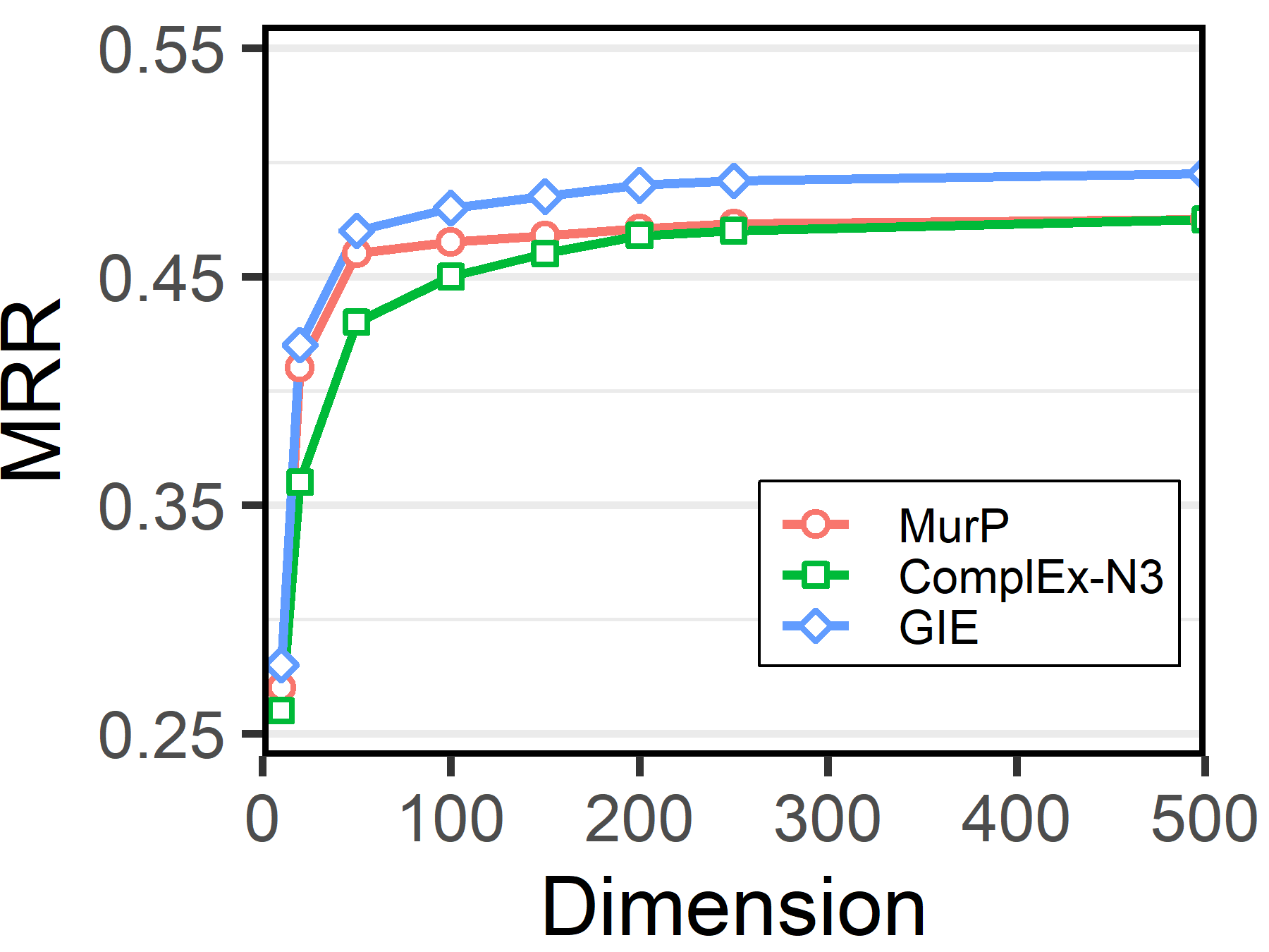
Figure 2: Impact of embedding dimension.

Impact of Embedding Dimension.

To understand the role of dimensionality, we conduct experiments on WN18RR against SOTA methods under varied dimensional settings $(10,20,50,100,150,200,250,500)$ shown in Figure 2. GIE can exploit hyperbolic, hyperspheric and Euclidean spaces jointly for knowledge graph embedding through an interaction learning mechanism, and we can see that GIE performs well in both low and high dimensions.

Model	RotatE	MuRP	GIE
WN18RR	40.95M	32.76M	17.65M ($\downarrow 46.1\%$)
FB15K237	29.32M	5.82M	3.41M ($\downarrow 41.4\%$)
YAGO3-10	49.28M	41.47M	23.81M ($\downarrow 42.6\%$)

Table 4: Number of free parameters comparison.

Number of Free Parameters Comparison.

We compare the numbers of parameters of RotatE and MuRP with that of GIE in the experiments above. Geometry interaction can learn a reliable spatial structure by geometric interaction, which reduce the dependence on adding dimensions to improve performance. As shown in Table 4, it obviously shows that GIE can maintain superior performance with fewer parameters.

Ablation Study on Geometry Interaction. In order to study the performance of each component in the geometry interaction score function Eq.(10) separately, we remove $d_{c}(\operatorname{Inter}(\bm{E_{t}},\bm{H_{t}},\bm{S_{t}}),\bm{h})$ of the score function and denote the model as GIE₁. We remove $d_{c}(\operatorname{Inter}(\bm{E_{h}},\bm{H_{h}},\bm{S_{h}}),\bm{t})$ of the score function and denote the model as GIE₂. We remove the geometry interaction process of the score function and denote the model as GIE₃. As shown in Table 6 in Appendix, GIE₁, GIE₂ and GIE₃ perform poorly compared to GIE. The experiment proves that the geometry interaction is a critical step for the embedding performance since geometric interaction is extremely beneficial for learning reliable spatial structures of KGs.

Conclusion

In this paper, we design a new knowledge graph embedding model named GIE that can exploit structures of knowledge graphs with interaction in Euclidean, hyperbolic and hyperspherical space simultaneously. Theoretically , GIE is advantageous with its capability in learning reliable spatial structure features in an adaptive way. Moreover, GIE can embrace rich and expressive semantic matching between entities and satisfy the key of relational representation learning. Empirical experimental evaluations on three well-established datasets show that GIE can achieve an overall the state-of-the-art performance, outperforming multiple recent strong baselines with fewer free parameters.

Appendix A Proof for Transformations of the Special Euclidean Group

We take a two-dimensional space as an example and the conclusion for higher dimensional space can be analogized accordingly.

Proof of reflection transformation. Denote $\theta$ as the angle of reflection. The reflection matrix can represent the reflection transformation, which is defined as follows:

$$\bm{M}_{Ref}=\left[\begin{array}[]{cc}\cos(\theta)&\sin(\theta)\\ \sin(\theta)&-\cos(\theta)\\ \end{array}\right].$$

Then we have $\bm{M}_{Ref}^{T}\bm{M}_{Ref}=\mathbf{I}$ and $\operatorname{det}\bm{M}_{Ref}=1$. It implies $\bm{M}_{Ref}\in\mathbf{SO}(n)$, so $\bm{M}_{Ref}\in\mathbf{SE}(n)$ hlods. Then the proof completes.

Proof of inversion transformation. According to Eq.(5), if a matrix $\bm{A}\in\mathbf{SO}(n)\in\mathbf{SE}(n)$, we have $\bm{A}^{T}\bm{A}=\mathbf{I}$ , then we can deduce $\bm{A}$ is an inversion matrix. Therefore it can represent the inversion transformation and the proof completes.

Proof of translation transformation. According to Eq.(6), if a matrix $\mathbf{A}=\left[\begin{array}[]{cc}\mathbf{R}&\mathbf{v}\\ 0&1\end{array}\right]\in\mathbf{SE}(n)$, we just make $\mathbf{R}$ be $\mathbf{0}$, then $\bm{A}$ is a translation matrix. The proof completes.

Proof of rotation transformation. Denote $\theta$ as the angle of rotation. The reflection matrix can represent the rotation transformation, which is defined as follows:

$$\bm{M}_{Rot}=\left[\begin{array}[]{cc}\cos(\theta)&-\sin(\theta)\\ \sin(\theta)&\cos(\theta)\\ \end{array}\right].$$

Then we have $\bm{M}_{Rot}^{T}\bm{M}_{Rot}=\mathbf{I}$ and $\operatorname{det}\bm{M}_{Rot}=1$. It implies $\bm{M}_{Rot}\in\mathbf{SO}(n)$, so $\bm{M}_{Rot}\in\mathbf{SE}(n)$ hlods. Then the proof completes.

Proof of homothety transformation. According to Eq.(6), if a matrix $\bm{A}\in\mathbf{SE}(n)$, we can turn it into a diagonal matrix, then it is a homothety matrix about itself. The proof completes.

Appendix B Proof of Key Patterns

As shown in Eq.(5), to simplify the notations, we take 2-dimensional space as an example, in which all involved embeddings are real. The conclusion in n-dimensional space can be analogized accordingly. For a given matrix $\bm{M}=\left[\begin{array}[]{cc}a&b\\ c&d\\ \end{array}\right]$, we set $\overline{\bm{M}}=\left[\begin{array}[]{cc}\frac{a}{\sqrt{a^{2}+b^{2}}}&\frac{b}{\sqrt{a^{2}+b^{2}}}\\ \frac{c}{\sqrt{c^{2}+d^{2}}}&\frac{d}{\sqrt{c^{2}+d^{2}}}\\ \end{array}\right]$. If $\overline{\bm{M}}\in\mathbf{G}\mathbf{L}(2,\mathbb{R})$, we have $ab+cd=0$. We might as well let $\overline{\bm{M}}$ satisfy the conditions of $\mathbf{G}\mathbf{L}(2,\mathbb{R})$ and denote it as $\bm{R}$. Then according to Eq.(6), we have the $\mathbf{A}=\left[\begin{array}[]{cc}\mathbf{R}&\mathbf{t}\\ 0&1\end{array}\right]$, where $\bm{t}\in\mathbb{R}^{2}$. The inverse of $\bm{A}$ is $\bm{A}^{-1}=\left[\begin{array}[]{cc}\bm{R}^{-1}&-\bm{R}^{-1}\bm{t}\\ 0&1\\ \end{array}\right]$. Note that since $\bm{R}\in\mathbf{G}\mathbf{L}(2,\mathbb{R})$, we have $\bm{R}^{-1}=\bm{R}^{\top}$, which means that the the reverse of $\bm{R}$ is always existing so the the reverse of $\bm{A}$ is always existing.

We denote $\otimes$ as the the multiplication in tangent space. Next we will prove the seven patterns hold in tangent space as follows.

Proof of symmetry pattern. To prove the symmetry pattern, if $\bm{r}(\bm{h},\bm{t})$ and $\bm{r}(\bm{t},\bm{h})$ hold, we have the equality as follows:

$$(\bm{t}=\bm{r}\otimes\bm{h})\wedge(\bm{h}=\bm{r}\otimes\bm{t})\Rightarrow\bm{r}\otimes\bm{r}=\bm{1}.$$

Proof of antisymmetry pattern. In order to prove the antisymmetry pattern, we need to prove the following inequality when $\bm{r}(\bm{h},\bm{t})$ and $\neg\bm{r}(\bm{t},\bm{h})$ hold:

$$(\bm{t}=\bm{r}\otimes\bm{h})\wedge(\bm{h}\neq\bm{r}\otimes\bm{t})\Rightarrow\bm{r}\otimes\bm{r}\neq\bm{1}.$$

Proof of inversion pattern. To prove the inversion pattern, if $\bm{r}_{1}(\bm{h},\bm{t})$ and $\bm{r}_{2}(\bm{t},\bm{h})$ hold, we have the equality as follows:

$$(\bm{t}=\bm{r}_{1}\otimes\bm{h})\wedge(\bm{h}=\bm{r}_{2}\otimes\bm{t})\Rightarrow\bm{r}_{1}=\bm{r}_{2}^{-1}.$$

Proof of composition pattern. In order to prove the antisymmetry pattern, we need to prove the following equality holds when $\bm{r}_{1}(\bm{h},\bm{p})$, $\bm{r}_{2}(\bm{h},\bm{t})$ and $\bm{r}_{3}(\bm{t},\bm{p})$ hold:

$$(\bm{p}=\bm{r}_{1}\otimes\bm{h})\wedge(\bm{t}=\bm{r}_{2}\otimes\bm{h})\wedge(\bm{p}=\bm{r}_{3}\otimes\bm{t})\Rightarrow\bm{r}_{1}=\bm{r}_{2}\otimes\bm{r}_{3}.$$

Proof of hierarchy pattern. First of all, the hyperbolic space used by our model can capture the hierarchical structure of the data. Next we prove that the model can also logically derive the hierarchy pattern. To prove the hierarchy pattern, if $\bm{r}_{1}(\bm{h},\bm{t})$ and $\bm{r}_{1}(\bm{h},\bm{t})$ hold, we need to prove the following equality holds:

$$\bm{r}_{1}(\bm{h},\bm{t})\Rightarrow\bm{r}_{2}(\bm{h},\bm{t}).$$

Then we need to prove

$$\bm{t}=\bm{r}_{1}\otimes\bm{h}\Rightarrow\bm{t}=\bm{r}_{2}\otimes\bm{h}.$$ (12)

We assume that the Eq.(12) holds, then we have

$$(\bm{t}=\bm{r}_{1}\otimes\bm{h})\wedge(\bm{t}=\bm{r}_{2}\otimes\bm{h})\Rightarrow\bm{r}_{1}\otimes\bm{h}=\bm{r}_{2}\otimes\bm{h}.$$ (13)

we denote $\bm{r}_{1}$ as $\left[\begin{array}[]{cc}\mathbf{R}_{1}&\mathbf{t}_{1}\\ 0&1\end{array}\right]$ and $\bm{r}_{2}$ as $\left[\begin{array}[]{cc}\mathbf{R}_{2}&\mathbf{t}_{2}\\ 0&1\end{array}\right]$, where $\bm{R}_{1}=\left[\begin{array}[]{cc}\frac{a_{1}}{\sqrt{a_{1}^{2}+b_{1}^{2}}}&\frac{b_{1}}{\sqrt{a_{1}^{2}+b_{1}^{2}}}\\ \frac{c_{1}}{\sqrt{c_{1}^{2}+d_{1}^{2}}}&\frac{d_{1}}{\sqrt{c_{1}^{2}+d_{1}^{2}}}\\ \end{array}\right]$ with $a_{1}b_{1}+c_{1}d_{1}=0$, $\bm{R}_{2}=\left[\begin{array}[]{cc}\frac{a_{2}}{\sqrt{a_{2}^{2}+b_{2}^{2}}}&\frac{b_{2}}{\sqrt{a_{2}^{2}+b_{2}^{2}}}\\ \frac{c_{2}}{\sqrt{c_{2}^{2}+d_{2}^{2}}}&\frac{d_{2}}{\sqrt{c_{2}^{2}+d_{2}^{2}}}\\ \end{array}\right]$ with $a_{2}b_{2}+c_{2}d_{2}=0$, $\bm{t}_{1}\in\mathbb{R}^{2}$ and $\bm{t}_{2}\in\mathbb{R}^{2}$. Then we bring $\bm{r}_{1}$ and $\bm{r}_{2}$ into the Eq.(13). Such we can get the solutions of $\bm{r}_{1}$ and $\bm{r}_{2}$ after solving the equation, which can satisfy the Eq.(12). Then we have $\bm{r}_{1}(\bm{x},\bm{y})\Rightarrow\bm{r}_{2}(\bm{x},\bm{y})$.

Proof of intersection pattern. In order to prove the intersection pattern, if $\bm{r}_{1}(\bm{h},\bm{t})$, $\bm{r}_{2}(\bm{h},\bm{t})$ and $\bm{r}_{3}(\bm{h},\bm{t})$ hold, we have the following equality:

$$(\bm{t}=\bm{r}_{1}\otimes\bm{h})\wedge(\bm{t}=\bm{r}_{2}\otimes\bm{h})\Rightarrow(\left[\begin{array}[]{cc}\mathbf{R}_{1}&\mathbf{v}_{1}\\ 0&1\end{array}\right]\otimes\left[\begin{array}[]{c}\bm{h}\\ 1\\ \end{array}\right]$$

$$= \left[\begin{array}[]{c}\bm{t}\\ 1\\ \end{array}\right])\wedge\left(\left[\begin{array}[]{cc}\mathbf{R}_{2}&\mathbf{v}_{2}\\ 0&1\end{array}\right]\otimes\left[\begin{array}[]{c}\bm{h}\\ 1\\ \end{array}\right]=\left[\begin{array}[]{c}\bm{t}\\ 1\\ \end{array}\right]\right).$$

Then we have

$$\bm{R}_{1}\otimes\bm{h}+\bm{v}_{1}=\bm{t},\ \bm{R}_{2}\otimes\bm{h}+\bm{v}_{2}=\bm{t}.$$

We multiply the left and right parts of the first equation by $\bm{v}_{2}$ respectively, and we multiply the left and right parts of the second equation by $\bm{v}_{1}$ respectively. Then we have:

$$\bm{v}_{2}\otimes\bm{R}_{1}\otimes\bm{h}+\bm{v}_{2}\otimes\bm{v}_{1}=\bm{v}_{2}\otimes\bm{t},\ \bm{v}_{1}\otimes\bm{R}_{2}\otimes\bm{h}+\bm{v}_{1}\otimes\bm{v}_{2}=\bm{v}_{1}\otimes\bm{t}.$$

Make the first formula subtract the second formula above, and we can get

$$(\bm{v}_{2}\otimes\bm{R}_{1}-\bm{v}_{1}\otimes\bm{R}_{2})\otimes\bm{h}=(\bm{v}_{2}-\bm{v}_{1})\otimes\bm{t}.$$

Since $\bm{r}_{1}\neq\bm{r}_{2}$, $v_{1}\neq v_{2}$. Then we have

$$(\bm{v}_{2}-\bm{v}_{1})^{-1}\otimes(\bm{v}_{2}\otimes\bm{R}_{1}-\bm{v}_{1}\otimes\bm{R}_{2})\otimes\bm{h}=\bm{t}.$$

Next let $\bm{r}_{3}=\left[\begin{array}[]{cc}\mathbf{R}_{3}&\bm{v}_{3}\\ 0&1\end{array}\right]$, where $\mathbf{R}_{3}=(\bm{v}_{2}-\bm{v}_{1})^{-1}\otimes(\bm{v}_{2}\otimes\bm{R}_{1}-\bm{v}_{1}\otimes\bm{R}_{2})$ and $\bm{v}_{3}=\bm{0}$. Then we have $\bm{r}_{1}(\bm{x},\bm{y})\wedge\bm{r}_{2}(\bm{x},\bm{y})\Rightarrow\bm{r}_{3}(\bm{x},\bm{y})$.

Proof of mutual exclusion pattern. To prove the mutual exclusion pattern, if $\bm{r}_{1}(\bm{h},\bm{t})$ and $\bm{r}_{2}(\bm{h},\bm{t})$ hold, where $\bm{r}_{1}$ and $\bm{r}_{2}$ are orthogonal ($\bm{r}_{1}$$\bm{r}_{2}=\bm{0}$), we have the formula as follows:

$$(\bm{t}=\bm{r}_{1}\otimes\bm{h})\wedge(\bm{t}=\bm{r}_{2}\otimes\bm{h})$$

$$\Rightarrow \bm{r}_{1}\otimes\bm{h}=\bm{r}_{2}\otimes\bm{h}$$

$$\Rightarrow \bm{r}_{1}\otimes\bm{r}_{1}\otimes\bm{h}=\bm{r}_{1}\otimes\bm{r}_{2}\otimes\bm{h}$$

$$\Rightarrow \bm{r}_{1}\otimes\bm{r}_{1}\otimes\bm{h}=\bm{0}$$

$$\Rightarrow \perp.$$

Therefore, we have $\bm{r}_{1}(\bm{x},\bm{y})\wedge\bm{r}_{2}(\bm{x},\bm{y})\Rightarrow\perp$.

Appendix C Hierarchy Estimates

There are two main metrics to estimate how hierarchical a relation is, which is called the curvature estimate $\xi_{G}$ (it means how much the graph is tree-like) and the Krackhardt hierarchy score Khs_G (it means how many small loops in the graph). Each of these two measures has its own merits: the global hierarchical behaviours can be captured by the curvature estimate, and the local behaviour can be captured by the Krackhardt score.

Curvature estimate. In order to estimate the curvature of a relation $r$, we restrict to the undirected graph $G_{r}$ spanned by the edges labeled as $r$. As shown in (Gu et al. 2019a), for the given vertices $\{a,b,c\}$, we denote $\xi_{G_{r}}(a,b,c)$ as the curvature estimate of a triangle in $G_{r}$, which can be given as follows:

$$\xi_{G_{r}}(a,b,c)= \frac{1}{2d_{G_{r}}(a,m)}\left(d_{G_{r}}(a,m)^{2}+d_{G_{r}}(b,c)^{2}/4\right.$$

$$-\left.\left(d_{G_{r}}(a,b)^{2}+d_{G_{r}}(a,c)^{2}\right)/2\right),$$

where $m$ denotes the midpoint of the shortest path from $b$ to $c$. For the triangle, its curvature estimate is positive if it is in circles; its curvature estimate is zero if it is in lines; its curvature estimate is negative if it is in trees. Moreover, following (Gu et al. 2019a), suppose there is a triangle in a Riemannian manifold $M$ lying on a plane, and we can use $\xi_{M}(a,b,c)$ to estimate the sectional curvature of the plane. Denote the total number of connected components in $G_{r}$ as $m_{r}$, denote the number of nodes in the component $c_{i,r}$ as $N_{i,r}$ and denote the mean of the estimated curvatures of the sampled triangles as $\xi_{G_{r}}$. We then sample 1000 $w_{i,r}$ triangles from each connected component $c_{i,r}$ of $G_{r}$ where $w_{i,r}=\frac{N_{i,r}^{3}}{\sum_{i=1}^{m_{r}}N_{i,r}^{3}}$. Next, we take the weighted average of the relation curvatures $\xi_{G_{r}}$ with respect to the weights $\frac{\sum_{i=1}^{m_{r}}N_{i,r}^{3}}{\sum_{r}\sum_{i=1}^{m_{r}}N_{i,r}^{3}}$ for all the graphs.

Krackhardt hierarchy score. For the directed graph $G_{r}$ which is spanned by the relation $r$, we denote the adjacency matrix ( If there is an edge connecting node $i$ to node $j$, we have $R_{i,j}=1$. If there is not an edge connecting node $i$ to node $j$, we have $R_{i,j}\neq 1$.) as $R$. Then we have:

$$\mathrm{Khs}_{G_{r}}=\frac{\sum_{i,j=1}^{n}R_{i,j}\left(1-R_{j,i}\right)}{\sum_{i,j=1}^{n}R_{i,j}}$$ (14)

More details can refer to (Everett and Krackhardt 2012). For fully observed symmetric relations, each edge of which is in a two-edge loop, it can be seen that Khs${}_{G_{r}}=0$. And for the anti-symmetric relations, we have Khs${}_{G_{r}}=1$.

relation name	$\xi_{G}$	Khs	MuRE	MuRP	MuRS	MuRMP	MuRMP-a	GIE
also$\_$see	-2.09	.24	.634	.705	.483	.692	.725	$\bm{.759}$
hypernym	-2.46	.99	.161	.228	.126	.222	.232	$\bm{.262}$
has$\_$part	-1.43	1	.215	.282	.301	.134	.316	$\bm{.334}$
member$\_$meronym	-2.90	1	.272	.346	.138	.343	$.350$	$\bm{.360}$
synset$\_$domain$\_$topic$\_$of	-0.69	.99	.316	.430	.163	.421	$\bm{.445}$	.435
instance$\_$hypernum	-0.82	1	.488	.471	.258	.345	.491	$\bm{.501}$
member$\_$of$\_$domain$\_$region	-0.78	1	.308	.347	.201	.344	.349	$\bm{.404}$
member$\_$of$\_$domain$\_$usage	-0.74	1	.396	.417	.228	.416	$.420$	$\bm{.438}$
derivationally$\_$related$\_$form	-3.84	0.4	.954	.967	.965	.967	$\bm{.970}$	$.968$
similar$\_$to	-1.00	0	$\bm{1}$	$\bm{1}$	$\bm{1}$	$\bm{1}$	$\bm{1}$	$\bm{1}$
verb$\_$group	-0.5	0	.974	.974	.976	.976	.981	$\bm{.984}$

Table 5: Comparison of hits@10 for WN18RR. MuRMP-a represents MuRMP-autoKT in (Wang et al. 2021).

	WN18RR				FB15k-237				YAGO3-10
Analysis	MRR	H@1	H@3	H@10	MRR	H@1	H@3	H@10	MRR	H@1	H@3	H@10
GIE1	.472	.438	.474	.534	.336	.231	.373	.526	.534	.477	.584	.680
GIE2	.477	.440	.483	.541	.338	.236	.371	.526	.538	.479	.588	.674
GIE3	.471	.436	.470	.531	.332	.228	.375	.523	.531	.473	.581	.671

Table 6: Analysis on different variants of scoring function.

Appendix D Experimental Details

We conduct the hyperparameter search for the negative sample size, learning rate, batch size, dimension and the number of epoch. We train each model for 150 epochs and use early stopping after 100 epochs if the validation MRR stops increasing. Moreover, we count the running time of each epoch of GIE on different datasets: 20s for WN18RR, 34s for FB15K237, 65s for YAGO3-10. We need to run 150 epochs in total. Therefore, the overall time for each datasets is between 50 minutes and 162 minutes.

In the test dataset, we measure and compare the performance of models listed in the paper for each test triplet $(h,r,t)$. For all $h^{\prime}\in\mathcal{E}$ (where $\mathcal{E}$ is the set of entities), we calculate the scores of triplets $(h^{\prime},r,t)$ and then denote the ranking of the triplet $(h,r,t)$ among these triplets as $rank_{h}$. Next, for all $t^{\prime}\in\mathcal{E}$, we compute the scores of triplets $(h,r,t^{\prime})$ and denote the ranking of the triplet $(h,r,t)$ among these triplets as $rank_{t}$. According to the calculation above, MRR is calculated as follows, which is the mean of the reciprocal rank for the test dataset:

$$MRR=\frac{1}{2*|\Omega|}\sum_{(h,r,t)\in\Omega}\frac{1}{rank_{h}(h,r,t)}+\frac{1}{rank_{t}(h,r,t)}.$$

where $\Omega$ denotes the set of observed triplets in the test dataset.

References

- Balazevic, Allen, and Hospedales (2019a) Balazevic, I.; Allen, C.; and Hospedales, T. M. 2019a. Hypernetwork Knowledge Graph Embeddings. In ICANN, 553–565.
- Balazevic, Allen, and Hospedales (2019b) Balazevic, I.; Allen, C.; and Hospedales, T. M. 2019b. Multi-relational Poincaré Graph Embeddings. In NeurIPS, 4465–4475.
- Balažević, Allen, and Hospedales (2019) Balažević, I.; Allen, C.; and Hospedales, T. M. 2019. Tucker: Tensor factorization for knowledge graph completion. In EMNLP, 5185–5194.
- Bansal et al. (2019) Bansal, T.; Juan, D.-C.; Ravi, S.; and McCallum, A. 2019. A2N: attending to neighbors for knowledge graph inference. In ACL, 4387–4392.
- Berant et al. (2013) Berant, J.; Chou, A.; Frostig, R.; and Liang, P. 2013. Semantic Parsing on Freebase from Question-Answer Pairs. In ACL, 1533–1544.
- Berant and Liang (2014) Berant, J.; and Liang, P. 2014. Semantic Parsing via Paraphrasing. In ACL, 1415–1425.
- Bordes et al. (2013) Bordes, A.; Usunier, N.; Garcia-Duran, A.; Weston, J.; and Yakhnenko, O. 2013. Translating embeddings for modeling multi-relational data. In NeurIPS, 2787–2795.
- Cao et al. (2021) Cao, Z.; Xu, Q.; Yang, Z.; Cao, X.; and Huang, Q. 2021. Dual Quaternion Knowledge Graph Embeddings. In AAAI, 6894–6902.
- Chami et al. (2020) Chami, I.; Wolf, A.; Juan, D.-C.; Sala, F.; Ravi, S.; and Ré, C. 2020. Low-Dimensional Hyperbolic Knowledge Graph Embeddings. In ACL.
- Dettmers et al. (2017) Dettmers, T.; Minervini, P.; Stenetorp, P.; and Riedel, S. 2017. Convolutional 2D Knowledge Graph Embeddings. In AAAI, 1811–1818.
- Diefenbach, Singh, and Maret (2018) Diefenbach, D.; Singh, K. D.; and Maret, P. 2018. WDAqua-core1: A Question Answering service for RDF Knowledge Bases. In WWW, 1087–1091.
- Dong et al. (2014) Dong, X.; Gabrilovich, E.; Heitz, G.; Horn, W.; and Zhang, W. 2014. Knowledge vault: A web-scale approach to probabilistic knowledge fusion. ACM.
- Ebisu and Ichise (2018) Ebisu, T.; and Ichise, R. 2018. TorusE: Knowledge Graph Embedding on a Lie Group. In AAAI, 1819–1826.
- Everett and Krackhardt (2012) Everett, M. G.; and Krackhardt, D. 2012. A second look at Krackhardt’s graph theoretical dimensions of informal organizations. Soc. Networks, 34(2): 159–163.
- Ganea, Bécigneul, and Hofmann (2018) Ganea, O.; Bécigneul, G.; and Hofmann, T. 2018. Hyperbolic Neural Networks. In NeurIPS, 5350–5360.
- Gong et al. (2020) Gong, J.; Wang, S.; Wang, J.; Feng, W.; Peng, H.; Tang, J.; and Yu, P. S. 2020. Attentional Graph Convolutional Networks for Knowledge Concept Recommendation in MOOCs in a Heterogeneous View. In SIGIR, 79–88.
- Gu et al. (2019a) Gu, A.; Sala, F.; Gunel, B.; and Ré, C. 2019a. Learning Mixed-Curvature Representations in Product Spaces. In ICLR.
- Gu et al. (2019b) Gu, A.; Sala, F.; Gunel, B.; and Re, C. 2019b. LEARNING MIXED-CURVATURE REPRESENTATIONS IN PRODUCTS OF MODEL SPACES. In ICLR.
- Guo et al. (2020) Guo, Q.; Zhuang, F.; Qin, C.; Zhu, H.; Xie, X.; Xiong, H.; and He, Q. 2020. A Survey on Knowledge Graph-Based Recommender Systems. CoRR, abs/2003.00911.
- He et al. (2017) He, H.; Balakrishnan, A.; Eric, M.; and Liang, P. 2017. Learning Symmetric Collaborative Dialogue Agents with Dynamic Knowledge Graph Embeddings. In ACL, 1766–1776.
- He et al. (2015) He, S.; Liu, K.; Ji, G.; and Zhao, J. 2015. Learning to represent knowledge graphs with gaussian embedding. In CIKM, 623–632.
- Ji et al. (2015) Ji, G.; He, S.; Xu, L.; Liu, K.; and Zhao, J. 2015. Knowledge Graph Embedding via Dynamic Mapping Matrix. In ACL, 687–696.
- Jin et al. (2021a) Jin, D.; Huo, C.; Liang, C.; and Yang, L. 2021a. Heterogeneous Graph Neural Network via Attribute Completion. In WWW, 391–400.
- Jin et al. (2021b) Jin, D.; Yu, Z.; Jiao, P.; Pan, S.; Yu, P. S.; and Zhang, W. 2021b. A Survey of Community Detection Approaches: From Statistical Modeling to Deep Learning. IEEE Transactions on Knowledge and Data Engineering, DOI: 10.1109/TKDE.2021.3104155.
- Keizer et al. (2017) Keizer, S.; Guhe, M.; Cuayáhuitl, H.; Efstathiou, I.; Engelbrecht, K.; Dobre, M. S.; Lascarides, A.; and Lemon, O. 2017. Evaluating Persuasion Strategies and Deep Reinforcement Learning methods for Negotiation Dialogue agents. In EACL, 480–484.
- Lacroix, Usunier, and Obozinski (2018) Lacroix, T.; Usunier, N.; and Obozinski, G. 2018. Canonical Tensor Decomposition for Knowledge Base Completion. In ICML, 2863–2872.
- Lin et al. (2015) Lin, Y.; Liu, Z.; Sun, M.; Liu, Y.; and Zhu, X. 2015. Learning entity and relation embeddings for knowledge graph completion. In AAAI, 2181–2187.
- Mahdisoltani, Biega, and Suchanek (2013) Mahdisoltani, F.; Biega, J.; and Suchanek, F. 2013. YAGO3: A Knowledge Base from Multilingual Wikipedias. In CIDR.
- Mahdisoltani, Biega, and Suchanek (2015) Mahdisoltani, F.; Biega, J.; and Suchanek, F. M. 2015. YAGO3: A Knowledge Base from Multilingual Wikipedias. In CIDR.
- Nathani et al. (2019) Nathani, D.; Chauhan, J.; Sharma, C.; and Kaul, M. 2019. Learning Attention-based Embeddings for Relation Prediction in Knowledge Graphs. In ACL, 4710–4723.
- Nguyen et al. (2018) Nguyen, D. Q.; Nguyen, T. D.; Nguyen, D. Q.; and Phung, D. 2018. A novel embedding model for knowledge base completion based on convolutional neural network. In NAACL-HLT, 327–333.
- Nickel, Rosasco, and Poggio (2016) Nickel, M.; Rosasco, L.; and Poggio, T. 2016. Holographic Embeddings of Knowledge Graphs. In AAAI, 1955–1961.
- Nickel, Tresp, and Kriegel (2011) Nickel, M.; Tresp, V.; and Kriegel, H. P. 2011. A Three-Way Model for Collective Learning on Multi-Relational Data. In ICML.
- Schlichtkrull et al. (2018) Schlichtkrull, M.; Kipf, T. N.; Bloem, P.; Van Den Berg, R.; Titov, I.; and Welling, M. 2018. Modeling relational data with graph convolutional networks. In ESWC, 593–607. Springer.
- Socher et al. (2013) Socher, R.; Chen, D.; Manning, C. D.; and Ng, A. Y. 2013. Reasoning With Neural Tensor Networks for Knowledge Base Completion. In NeurIPS.
- Sun et al. (2019) Sun, Z.; Deng, Z.; Nie, J.; and Tang, J. 2019. RotatE: Knowledge Graph Embedding by Relational Rotation in Complex Space. In ICLR, 1–18.
- Tang et al. (2020) Tang, Y.; Huang, J.; Wang, G.; He, X.; and Zhou, B. 2020. Orthogonal Relation Transforms with Graph Context Modeling for Knowledge Graph Embedding. In ACL, 2713–2722.
- Trouillon et al. (2016) Trouillon, T.; Welbl, J.; Riedel, S.; Gaussier, E.; and Bouchard, G. 2016. Complex embeddings for simple link prediction. In ICML, 2071–2080.
- Wang et al. (2021) Wang, S.; Wei, X.; dos Santos, C. N.; Wang, Z.; Nallapati, R.; Arnold, A.; Xiang, B.; Philip, S. Y.; and Cruz, I. F. 2021. Mixed-Curvature Multi-Relational Graph Neural Network for Knowledge Graph Completion. In WWW.
- Wang et al. (2014) Wang, Z.; Zhang, J.; Feng, J.; and Chen, Z. 2014. Knowledge graph embedding by translating on hyperplanes. In AAAI, 1112–1119.
- Xiao, Huang, and Zhu (2016a) Xiao, H.; Huang, M.; and Zhu, X. 2016a. From One Point to a Manifold: Knowledge Graph Embedding for Precise Link Prediction. In IJCAI, 1315–1321.
- Xiao, Huang, and Zhu (2016b) Xiao, H.; Huang, M.; and Zhu, X. 2016b. TransG: A generative model for knowledge graph embedding. In ACL, 2316–2325.
- Yang et al. (2015) Yang, B.; Yih, W.; He, X.; Gao, J.; and Deng, L. 2015. Embedding Entities and Relations for Learning and Inference in Knowledge Bases. In ICLR, 1–13.
- Yu et al. (2021) Yu, Z.; Jin, D.; Liu, Z.; He, D.; Wang, X.; Tong, H.; and Han, J. 2021. AS-GCN: Adaptive Semantic Architecture of Graph Convolutional Networks for Text-Rich Networks. In ICDM.
- Zhang et al. (2019) Zhang, S.; Tay, Y.; Yao, L.; and Liu, Q. 2019. Quaternion knowledge graph embeddings. In NeurIPS, 2731–2741.