Speech Quality Assessment through MOS using Non-Matching References

Abstract

Human judgments obtained through Mean Opinion Scores (MOS) are the most reliable way to assess the quality of speech signals. However, several recent attempts to automatically estimate MOS using deep learning approaches lack robustness and generalization capabilities, limiting their use in real-world applications. In this work, we present a novel framework, NORESQA-MOS, for estimating the MOS of a speech signal. Unlike prior works, our approach uses non-matching references as a form of conditioning to ground the MOS estimation by neural networks. We show that NORESQA-MOS provides better generalization and more robust MOS estimation than previous state-of-the-art methods such as DNSMOS [1] and NISQA [2], even though we use a smaller training set. Moreover, we also show that our generic framework can be combined with other learning methods such as self-supervised learning and can further supplement the benefits from these methods.

Index Terms: speech quality, non-matching reference, Mean Opinion Score, no-reference metrics, speech enhancement

1 Introduction

Quality assessment of speech signals plays a critical role in many applications. The gold standard for assessment of speech quality is subjective judgments by humans. Often, these subjective judgments are made by conducting different listening tests. Mean Opinion Score (MOS) [3] is the “de-facto” metric to assess speech quality through listening tests. However, such subjective evaluations are time and resource consuming, especially when repeated many times per recording, and are therefore not scalable. Moreover, to obtain MOS reliably, one needs to control listening environments and hardware appropriately, further adding to the constraints of conducting MOS tests. This has led to considerable effort in developing alternatives to MOS tests.

One class of alternatives that have been developed are full-reference objective methods, e.g. PESQ[4], POLQA[5] and VISQOL[6]), to mention a few. While these objective metrics remove the heavy workload of subjective listening tests, they correlate with MOS to a limited degree [7, 8, 9]. More importantly, their effectiveness is usually limited to specific speech applications and becomes obsolete with the emergence of new scenarios [10, 11]. Even more inhibiting is the reliance of these objective metrics on a clean, reference speech signal for computing an assessment rating.

A recent class of alternatives is provided by deep-learning-based systems, which offer scalable and rapidly re-trainable solutions that are expandable to many speech and audio-related tasks [12, 13, 14, 15, 16, 17, 18]. Several of these methods estimate the aforementioned objective metrics (e.g. PESQ [4]) directly, without using any reference. More significantly, there have also been attempts to learn the mapping between audio signals and MOS directly.

The task of developing machine learning methods for MOS estimation is quite challenging. MOS captures the complex and multi-dimensional nature of quality perception in humans [19]. However, several aspects of human auditory perception are not yet fully understood. This makes it tricky to design MOS estimation methods, and often the idea is to rely on labeled MOS datasets for training neural networks in a supervised manner [14, 15, 2, 9, 20, 1, 21, 22]. However, collecting large scale MOS datasets to train deep learning models is challenging too. Current MOS datasets are often limited to specific domains, e.g. Text-to-Speech (TTS) and Voice Conversion in BVCC [23], telephony distortions in NISQA [2], and speech enhancement distortions in DNSMOS [1]. Moreover, MOS tests are difficult to conduct and crowd-sourced MOS can have considerable label noise [1]. These limitations make it harder to train models that can generalize well across various test conditions and applications [24, 25, 9], and the real-world uses of these MOS estimation methods remain limited.

A potential solution to above constraints can be self-supervised learning (SSL). SSL methods leverage large unlabeled data for learning models that can be utilized in other tasks with sparse labeled data. Cooper et al. [9] proposed the same for MOS estimation by using large pretrained audio models learned using SSL methods (e.g. wav2vec2.0 [26] and HuBERT [27]).

Another recent novel framework for quality assessment is NORESQA [25] (NOn-matching REference based Speech Quality Assessment). Motivated by human’s ability to compare the quality of two speech signals of different content, NORESQA proposed speech quality assessment by learning to predict a relative quality score for a given speech recording with respect to any provided reference, irrespective of the differences in content, speaker’s language or gender. The non-matching references (NMRs) in NORESQA provide better grounding for the neural networks through conditioning by arbitrary speech signals of known quality. However, NORESQA was trained to predict Signal to Noise Ratio (SNR) and Scale invariant signal to distortion ratio (Si-SDR) for quality assessment.

In this paper, we propose NORESQA-MOS - a novel MOS estimation method built on the principles of NORESQA. Unlike prior works which are entirely reference-free, NORESQA-MOS relies on random NMRs of known qualities/MOS (either from a labeled dataset, or a clean set). We show that using our approach to compute relative MOS ratings leads to high generalization across in-domain and out-of-domain datasets. Moreover, combining NORESQA-MOS with other useful approaches (e.g. SSL pretraining) provides computational benefits by enabling smaller models to achieve significantly better generalization for MOS prediction. NORESQA-MOS is usable in real-world applications as any other reference-free approach as one can choose any set of speech recordings as NMR inputs to the network.

2 The NORESQA-MOS Framework

Our framework, NORESQA-MOS is designed to assess the MOS of a given speech recording using Non-Matching References (NMRs). The model takes in two recordings as inputs: a test recording $x_{\mathtt{test}}$ and another randomly chosen recording $x_{\mathtt{ref}}$. Fig 1 is a simple illustration of the model. Overall, given two input signals, our model predicts two outputs: i) a preference output suggesting which input is cleaner than the other, and ii) a relative MOS rating between the two inputs.

2.1 Framework Design and Model Architectures

NORESQA-MOS architecture (Fig 1) comprises three modules: a base model block, a downsampling block, and task specific output heads (preference and relative MOS prediction blocks).

Base model block: We consider two types of base model blocks: one where the base model is trained from scratch and another where the base model block is a pre-trained SSL model from Fairseq [28]. Overall, we train 3 different models with same architectural design (based on wav2vec2.0 [26]) but varying model capacity: (i) Scratch: same model architecture as wav2vec2.0, but less number of blocks, and consists of roughly 120k parameters; (ii) SSL-Small: mid-size pretrained SSL wav2vec2.0 model (“wav2vec_base”) consisting of roughly 91M parameters, and (iii) SSL-Big: large pretrained SSL wav2vec2.0 model (“wav2vec_big”) consisting of roughly 315M parameters.

Downsampling block: Consists of a fully connected layer that outputs 32 dimensional representations for each time-frame. The learnable parameters across these blocks are shared between the two inputs to our model. Finally, the embeddings for both inputs are concatenated, and passed on to the next blocks.

The next blocks consist of output heads for the training tasks, and are described below along with the training loss functions.

2.2 Training Tasks and Loss Functions

We follow a multi-task learning framework where we train our network on two tasks simultaneously: i) a  preference task, and ii) quantification task using a multi-task learning (MTL) [29] framework. Both output heads use attention pooling [2] to aggregate frame-level outputs to recording-level outputs. It mimics the selective auditory attention [30] properties due to which quality cannot be estimated using simple averaging.

Preference Task is designed such that the network learns to model which of the two inputs is “preferred” by humans. It is formulated as a binary classification problem. Let $\mathbf{x}_{ij}=(x_{i},x_{j})$ be an ordered pair input to the network, with $x_{i}$ as first input and $x_{j}$ as second input. Let $\text{MOS}_{x_{i}}$ and $\text{MOS}_{x_{j}}$ be the MOS ratings of $x_{i}$ and $x_{j}$ respectively. The goal is to predict the probability, $\mathbf{p}_{ij}$, of $x_{i}$ having better rating than $x_{j}$. More formally, the label $\mathbf{y}_{ij}$ for $\mathbf{x}_{ij}$ is a 2 dimensional, one-hot vector, with $\mathbf{y}_{ij}=[1,0]$ if $\text{MOS}_{x_{i}}>\text{MOS}_{x_{j}}$, and $\mathbf{y}_{ij}=[0,1]$ otherwise. The loss function is:

$$L_{P}(\mathbf{x}_{ij},\mathbf{y}_{ij})=\sum_{k=1}^{2}{-y^{k}_{ij}\log(p^{k}_{ij})}\vspace{-0.05in}$$ (1)

Relative Rating Task is designed to quantify the quality difference (MOS) between $x_{i}$ and $x_{j}$. The goal of this task is to predict the relative MOS ratings, ${\Delta}\text{MOS}_{ij}=\mathbf{s}_{ij}=|\text{MOS}_{x_{i}}-\text{MOS}_{x_{j}}|$. Let $\mathbf{r}_{ij}$ be the recording level relative MOS rating predicted by this output head. We then use L1 loss between $\mathbf{r}_{ij}$ and the target relative MOS $\mathbf{s}_{ij}$ to train the network:

$$L_{Q}(\mathbf{x}_{ij},\mathbf{s}_{ij})=\|r_{ij}-s_{ij}\|_{1}\vspace{-0.05in}$$ (2)

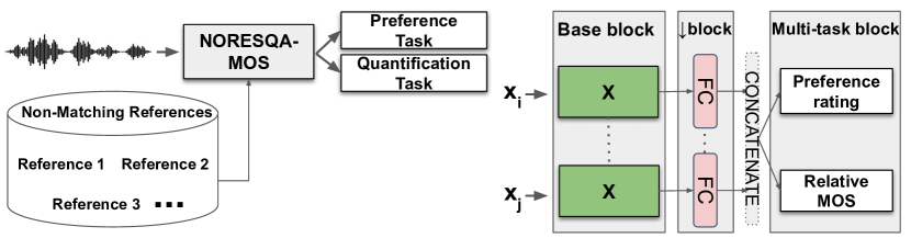
Figure 1: Left: NORESQA-MOS Framework: takes a test recording, and a randomly chosen NMR from a set and solves a preference and a quantification task. Right: NORESQA-MOS Architecture: takes two inputs ($x_{i}$ and $x_{j}$), passes through a base model ($X$ = scratch or pretrained wav2vec2.0), and outputs: (i) which recording is cleaner (preference-task); and (ii) relative MOS score (quantitative-task).

2.3 Training procedure

We assume the availability of a small labeled dataset of audio recordings, and their MOS ratings $\mathcal{D}_{\text{lab}}$. We also assume the availability of a clean speech database $\mathcal{D}_{\text{clean}}$.

The training input for the network, $\mathbf{x}_{ij}$, is created by sampling two recordings $x^{\prime}_{i}$ and $x^{\prime}_{j}$ (having MOS ratings $s_{i}$ and $s_{j}$ respectively) from $\mathcal{D}_{\text{lab}}$. Also note that $x^{\prime}_{i}$ and $x^{\prime}_{j}$ can also be sampled from $\mathcal{D}_{\text{clean}}$ whose rating is assumed to be the perfect MOS ($s_{i}$,$s_{j}$ = 5). Next, given $x^{\prime}_{i}$ and $x^{\prime}_{j}$, we apply data augmentations on the recordings including waveform inversion, audio reversal, and time stretching. Typically, it has been found that data augmentation improves performance, especially in situations that have sparse labeled examples [31]. All these augmentations are chosen such that they have none to minimal effect on MOS ratings, and training with these augmentations improve performance. For each recording, we sample a perturbation from the list above, and apply the perturbation at a randomly selected level to get recordings $x_{i}$, and $x_{j}$ respectively. Once we have the signals ($x_{i}$ and $x_{j}$) and their respective MOS ratings $s_{i}$ and $s_{j}$, we can train the network as described in Sec 2.2.

2.4 Usage: MOS Prediction

Once the network is trained, we can predict the MOS of a test input $x_{\text{test}}$ with respect to any reference $x_{\text{ref}}$. As already mentioned, this reference need not be the matching clean reference. To obtain the “absolute” quality, we select multiple clean NMRs (from $\mathcal{D}_{\text{clean}}$) with the assumption of perfect MOS ratings. We average the relative-rating block outputs over multiple NMRs to obtain a lower variance estimate of MOS.

3 Experimental Setup

3.1 Datasets and training

The clean NMR set ($\mathcal{D}_{\text{clean}}$) comes from the DAPS dataset [32]. The labeled MOS dataset ($\mathcal{D}_{\text{lab}}$) comes from BVCC [33]. It combines audio recordings from past years’ Blizzard Challenge for TTS and the Voice Conversion Challenge, with each recording being rated by 8 independant raters. Overall, it contains roughly 7000 audio recordings, and their corresponding MOS ratings. We use the pre-created training/development/test splits as provided by the VOICEMOS challenge organizers.

The inputs to our model are 3 seconds waveform excerpts. We use the Adam optimizer with a learning rate of $10^{-4}$ with a batch size of 64. We train the network for 1000 epochs. We also use n=100 NMRs for all evaluations.

3.2 Baselines

We compare our approach to state-of-the-art no-reference approaches like DNSMOS [1] and NISQA [2]. Moreover, for a fair comparison and to demonstrate effectiveness of our NMR based approach, we also compare it with a model that is exactly same as ours but predicts the absolute MOS directly (D-MOS, short for Direct-MOS). Also note that all models are evaluated at 16kHz except NISQA which predicts MOS at 48kHz.

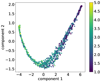
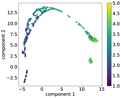
(a) PCA	(b) UMAP

Figure 2: Embedding Visualization: (a) PCA visualization showing local structure; and (b) UMAP visualization showing global structure. Plots show that the embeddings captures audio quality information.

4 Results

4.1 Objective evaluations

We conduct two objective evaluations to understand the embedding space learnt by NORESQA-MOS. We first look at how well the model clusters audio recordings of similar MOS ratings. Next, we visualize the embedding space of NORESQA-MOS to see if the model learns local or global structure.

Quality based retrieval: Here we consider the outputs after the base model block as the quality embeddings, and use it for quality based retrievals. Similar to [25], we first create a test dataset of 1000 recordings at 10 discrete quality levels (from 1 to 5). We take randomly selected queries and calculate the number of correct class instances in the top $K$ retrievals. We report the mean of this metric over all queries ($\text{MP}^{k}$). NORESQA-MOS gets $\text{MP}^{k=10}$ = 0.92, as compared to D-MOS $\text{MP}^{k=10}$ = 0.85, suggesting that our approach better clusters quality level groups in this learnt space.

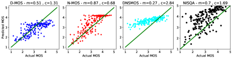
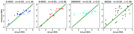
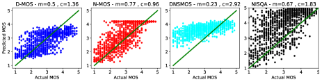
(a) In-Domain Task	(b) Out-of-Domain Task

Figure 3: Scatter plots: Top Row: System level predictions across the in-domain and out-of-domain tasks of the VOICEMOS challenge dataset (BVCC). Bottom Row: Utterance level predictions across the same dataset and tasks. We show comparisons across D-MOS, NORESQA-MOS, DNSMOS, and NISQA. Green line depicts $y=x$. Each plot title shows the slope (m) and intercept (c) of fitting a linear curve over the points.

Type	Name	HiFiGAN [34]			VoCo [35]			FFTnet [36]			BWE [37]			Dereverb [38]
		MSE$\downarrow$	PC$\uparrow$	SC$\uparrow$	MSE$\downarrow$	PC$\uparrow$	SC$\uparrow$	MSE$\downarrow$	PC$\uparrow$	SC$\uparrow$	MSE$\downarrow$	PC$\uparrow$	SC$\uparrow$	MSE$\downarrow$	PC$\uparrow$	SC$\uparrow$
Non-Int.	DNSMOS	0.18	0.97	0.92	0.57	0.70	0.41	0.21	0.66	0.60	1.58	0.65	0.61	2.25	0.70	0.79
	NISQA	0.40	0.94	0.90	1.44	0.63	0.29	0.53	0.53	0.48	2.44	0.69	0.67	1.92	0.80	0.81
1-17 D-MOS	Scratch	0.89	0.20	0.29	1.26	0.23	0.31	0.32	-0.12	-0.16	1.60	0.59	0.66	2.58	0.08	0.07
	SSL-small	0.68	0.68	0.71	0.68	0.22	0.12	0.64	0.45	0.50	0.96	0.44	0.42	1.95	0.13	0.05
	SSL-big	0.17	0.85	0.76	1.08	0.27	0.37	1.81	0.21	0.11	2.27	-0.03	-0.1	2.71	-0.27	-0.18
1-17 NORESQA-MOS	Scratch	0.14	0.23	0.30	0.68	0.57	0.55	0.29	0.12	0.07	0.45	0.71	0.80	1.21	0.70	0.71
	SSL-small	0.14	0.94	0.96	0.59	0.50	0.40	0.19	0.74	0.72	0.61	0.59	0.57	0.91	0.71	0.73
	SSL-big	0.10	0.90	0.83	0.73	0.83	0.60	0.18	0.74	0.78	1.64	0.81	0.81	0.54	0.20	0.10

Table 1: System-level-predictions (1): for NORESQA-MOS, D-MOS, DNSMOS, and NISQA. Mean Square Error (MSE), Spearman (SC), Pearson (PC) correlations are shown. NORESQA-MOS  is obtained using $n=100$ NMRs. $\uparrow$ or $\downarrow$ is better.

Embedding visualization: We visualize how the embedding space looks by projecting the embeddings to a 2D space (Fig 2) using dimensionality reduction techniques like PCA [39] and UMAP [40]. Similar to Manocha et al. [25] we see that the embeddings are more tightly clustered together for higher quality recordings. However, we do not observe two piece-wise linear functions - for low and high quality respectively as in [25]. Instead, we see a continuous projection curve which suggests that the manifold of speech recordings mapped to MOS ratings is smooth without any discontinuities. However, this trend is expected, given the subjective nature of MOS.

Type	Name	TCD_VOIP [41]			SASSEC [42]			SiSEC08 [43]			SiSEC18 [42]			SAOC [44]
		MSE$\downarrow$	PC$\uparrow$	SC$\uparrow$	MSE$\downarrow$	PC$\uparrow$	SC$\uparrow$	MSE$\downarrow$	PC$\uparrow$	SC$\uparrow$	MSE$\downarrow$	PC$\uparrow$	SC$\uparrow$	MSE$\downarrow$	PC$\uparrow$	SC$\uparrow$
Non-Int.	DNSMOS	0.71	0.96	0.96	1.37	0.74	0.81	1.24	0.54	0.56	1.06	0.22	0.23	1.45	0.64	0.64
	NISQA	0.32	0.95	0.93	0.44	0.85	0.83	1.34	0.61	0.66	1.13	0.09	0.08	1.15	0.67	0.62
1-17 D-MOS	Scratch	1.10	-0.21	-0.19	4.13	-0.32	-0.30	3.57	-0.34	0.05	3.31	-0.05	-0.20	4.00	-0.27	-0.05
	SSL-small	0.36	0.85	0.84	0.95	0.86	0.82	1.18	0.72	0.43	1.13	0.01	0.05	1.23	0.80	0.60
	SSL-big	1.34	0.10	0.05	0.81	0.73	0.52	0.82	0.01	0.33	0.95	0.12	0.21	0.85	0.47	0.30
1-17 NORESQA-MOS	Scratch	0.87	0.36	0.52	1.97	0.41	0.34	2.11	0.45	0.30	0.88	0.12	0.08	1.39	0.26	0.26
	SSL-small	0.26	0.87	0.87	0.17	0.95	0.90	0.80	0.73	0.56	0.97	0.30	0.25	0.79	0.89	0.80
	SSL-big	1.17	0.62	0.34	0.41	0.95	0.81	0.66	0.69	0.36	0.71	0.20	0.25	0.59	0.84	0.60

Table 2: System-level-predictions (2): for NORESQA-MOS, D-MOS, DNSMOS, and NISQA. Mean Square Error (MSE), Spearman (SC), Pearson (PC) correlations are shown. NORESQA-MOS  is obtained using $n=100$ NMRs. $\uparrow$ or $\downarrow$ is better.

Type	Name	PEASS_db [42]			HiFi2_Ted [45]			HiFi2_DAPS [45]			VoiceMOS_Main [33]			VoiceMOS_OOD [33]
		MSE$\downarrow$	PC$\uparrow$	SC$\uparrow$	MSE$\downarrow$	PC$\uparrow$	SC$\uparrow$	MSE$\downarrow$	PC$\uparrow$	SC$\uparrow$	MSE$\downarrow$	PC$\uparrow$	SC$\uparrow$	MSE$\downarrow$	PC$\uparrow$	SC$\uparrow$
Non-Int.	DNSMOS	1.16	0.55	0.71	1.14	0.96	0.94	0.26	0.81	0.73	0.72	0.78	0.78	0.75	0.64	0.62
	NISQA	0.26	0.36	0.25	1.19	0.94	0.94	0.91	0.76	0.72	1.06	0.67	0.71	0.70	0.60	0.54
1-17 D-MOS	Scratch	3.66	0.21	0.26	0.30	0.65	0.47	0.39	0.43	0.23	0.88	0.19	0.24	0.29	0.42	0.69
	SSL-small	0.96	0.46	0.42	0.36	0.96	0.93	0.22	0.92	0.95	0.20	0.85	0.89	0.09	0.96	0.96
	SSL-big	0.81	0.49	0.29	0.60	0.49	0.64	0.41	0.68	0.58	0.34	0.73	0.70	0.26	0.87	0.80
1-17 NORESQA-MOS	Scratch	0.94	0.26	0.31	0.16	0.79	0.49	0.32	0.88	0.65	0.67	0.21	0.24	0.23	0.49	0.78
	SSL-small	0.78	0.64	0.79	0.15	0.98	0.94	0.14	0.93	0.94	0.17	0.89	0.87	0.04	0.98	0.96
	SSL-big	0.65	0.52	0.57	0.46	0.51	0.78	0.32	0.85	0.81	0.33	0.81	0.80	0.14	0.89	0.85

Table 3: System-level-predictions (3): for NORESQA-MOS, D-MOS, DNSMOS, and NISQA. Mean Square Error (MSE), Spearman (SC), Pearson (PC) correlations are shown. NORESQA-MOS  is obtained using $n=100$ NMRs. $\uparrow$ or $\downarrow$ is better.

Type	Name	FFTnet [34]			SiSEC18 [35]			PEASS_db [36]			VoiceMOS_Main [37]			VoiceMOS_OOD [38]
		MSE $\downarrow$	PC$\uparrow$	SC$\uparrow$	MSE$\downarrow$	PC$\uparrow$	SC$\uparrow$	MSE$\downarrow$	PC$\uparrow$	SC$\uparrow$	MSE$\downarrow$	PC$\uparrow$	SC$\uparrow$	MSE$\downarrow$	PC$\uparrow$	SC$\uparrow$
Non-Int.	DNSMOS	0.41	0.40	0.41	1.93	0.16	0.13	2.07	0.08	0.08	1.03	0.61	0.60	0.88	0.44	0.44
	NISQA	0.92	0.37	0.25	2.56	0.10	0.05	1.38	0.12	0.11	1.45	0.62	0.63	1.12	0.43	0.33
1-17 D-MOS	Scratch	0.49	-0.02	-0.01	3.87	-0.05	-0.06	4.47	0.09	0.03	1.24	0.15	0.10	1.24	0.14	0.10
	SSL-small	0.97	0.22	0.23	2.23	-0.19	-0.14	1.77	-0.10	-0.07	0.34	0.80	0.84	0.34	0.84	0.34
	SSL-big	2.24	0.08	0.14	2.35	0.08	0.12	3.11	0.08	0.06	0.43	0.71	0.70	0.47	0.74	0.66
1-17 NORESQA-MOS	Scratch	0.31	0.01	0.02	1.64	0.14	0.13	1.76	0.14	0.12	0.88	0.18	0.13	1.02	0.28	0.19
	SSL-small	0.72	0.36	0.36	1.12	0.20	0.20	1.16	0.18	0.13	0.31	0.83	0.83	0.29	0.85	0.81
	SSL-big	0.50	0.51	0.48	2.09	0.16	0.12	2.73	0.10	0.06	0.47	0.76	0.73	0.43	0.76	0.73

Table 4: Utterance-level-predictions: for NORESQA-MOS, D-MOS, DNSMOS, and NISQA. Mean Square Error (MSE), Spearman (SC), Pearson (PC) correlations are shown. NORESQA-MOS  is obtained using $n=100$ NMRs. $\uparrow$ or $\downarrow$ is better.

4.2 Subjective evaluations

We evaluate MOS prediction through an exhaustive set of 16 different datasets. These datasets come from a variety of speech applications including speech synthesis (VoCo [35], FFTnet [36]), speech enhancement (Dereverberation [38], HiFi-GAN [34], HiFi-GAN2 [45]), audio source separation (SASSEC [42], SiSEC08 [43], SiSEC18 [42], SAOC [44]), telephony degradations (TCD_VOIP [41]), bandwidth extension (BWE [37]), and Voice Conversion and TTS (BVCC [23]). For more information on the datasets, please refer to Manocha et al. [46]. Our goal is to establish the generalization capabilities of all methods by evaluating on these diverse datasets.

Similar to prior works, we measure performance through Mean Square Errors (MSE), Pearson Correlation Coefficient (PC), and Spearman’s Rank Order Correlation (SC) of our predicted MOS with the MOS ratings from each dataset.

The NMRs for NORESQA-MOS are selected randomly from DAPS dataset [32]. For NORESQA-MOS, all experiments are repeated 10 times and averaged results with standard deviations are reported. We report both system level (averaged over ratings per system), as well as the utterance level predictions.

Scatter plots Fig 3 shows the performance of various metrics on a common dataset (BVCC) at a system level, and at an utterance level on in-domain and out-of-domain tasks.

We see that NORESQA-MOS correlates better than existing baselines including D-MOS. Looking at system level ratings, our approach has a smaller variance spread as compared to baseline approaches. Next, looking at utterance level ratings, we see that baseline approaches have either higher variance (NISQA and D-MOS) or high bias (DNSMOS). This broadly suggests the usefulness of our approach over existing approaches.

System level MOS predictions Results are displayed in Tables 1, 2 and 3. We note a few key observations from the these Tables. First, we note that NORESQA-MOS performs better than D-MOS across all three model classes. We attribute this to our NMR strategy that encourages learning content agnostic quality features. For e.g., specifically for Dereverb - D-MOS models fare worse than NORESQA-MOS because they fail to give reliable estimates, esp. under unseen, reverberant environments. In contrast, NORESQA-MOS performs better since it was trained to be content agnostic to learn quality features. Secondly, we also observe that generalization across unseen datasets generally increase with larger pretrained SSL models (e.g. HiFi-GAN, SASSEC, SiSEC08, SiSEC18, SAOC etc.). However, in a few cases, the performance drops as larger pretrained models are used, esp. for D-MOS. However, our NORESQA-MOS approach produces more consistent ratings across model capacities. Third, we note that NORESQA-MOS with the SSL-Small model generalizes better than D-MOS learning with SSL-Big as base modules. This shows the usefulness of our approach in training efficient models (i.e. with 1/4 the number of trainable parameters) that generalize well, and are faster to train and infer. Fourth, NORESQA-MOS approach scores higher than baseline approaches like DNSMOS and NISQA in terms of lower errors (MSE) and higher correlations, especially on challenging datasets like BWE which have subtle differences. The standard deviations for all datasets across Tables 1, 2, and 3 are consistently small ($\sim$0.02 rating) suggesting invariance to a particular NMR set. Moreover, NORESQA-MOS uses a fraction of the labeled examples for training compared to DNSMOS or NISQA and therefore is more effective for sparse labeled tasks. Finally, we note that our NMRs based MOS estimation approach improves performance across all model classes, whether training from scratch, or starting from a pretrained model across various model capacities. It shows that our approach is a generic way to improve MOS estimation and can be used to improve robustness of any model.

Utterance level MOS predictions We report results on a subset of datasets from the previous section due to space limitations.

Results are shown in Table 4. We see that NORESQA-MOS scores consistent correlations, and lowest errors amongst different datasets considered. Moreover, the standard deviations for datasets across Table 4 are small ($\sim$0.15 rating), and should further decrease as more NMRs are introduced. This suggests the usefulness of our approach to reducing variance in the ratings further. Utterance level MOS predictions have been identified as challenging for existing models [9]. Our NORESQA-MOS approach can produce more consistent ratings and improves performances almost across all datasets.

5 Conclusions and future work

In this paper, we presented NORESQA-MOS - a novel approach for MOS estimation of speech signals which uses non-matching references. It is motivated by human’s ability to assess quality independent of the speech content. We show that our method generalizes well to out-of-domain datasets and outperforms prior works trained on much larger datasets. Moreover, it provides good generalization with smaller models, making it more suitable for real-world uses. In the future, we would like to include more attributes including noisiness and coloration.

References

- [1] C. K. Reddy, V. Gopal, and R. Cutler, “DNSMOS: A non-intrusive perceptual objective speech quality metric to evaluate noise suppressors,” ICASSP, 2020.
- [2] G. Mittag, B. Naderi, A. Chehadi et al., “NISQA: A deep CNN-self-attention model for multidimensional speech quality prediction with crowdsourced datasets,” in Interspeech, 2021.
- [3] R. C. Streijl, S. Winkler, and D. S. Hands, “Mean opinion score (MOS) revisited: methods and applications, limitations and alternatives,” Multimedia Systems, vol. 22, no. 2, pp. 213–227, 2016.
- [4] A. W. Rix, J. G. Beerends, M. P. Hollier et al., “Perceptual evaluation of speech quality (PESQ)-a new method for speech quality assessment of telephone networks and codecs,” in 2001 IEEE ICASSP, vol. 2. IEEE, 2001, pp. 749–752.
- [5] J. G. Beerends, C. Schmidmer, J. Berger et al., “Perceptual objective listening quality assessment (POLQA), the third generation itu-t standard for end-to-end speech quality measurement part i—temporal alignment,” Journal of the AES, vol. 61, no. 6, pp. 366–384, 2013.
- [6] A. Hines, J. Skoglund, A. C. Kokaram et al., “ViSQOL: an objective speech quality model,” EURASIP Journal on Audio, Speech, and Music Processing, vol. 2015, no. 1, pp. 1–18, 2015.
- [7] E. Cano, D. FitzGerald, and K. Brandenburg, “Evaluation of quality of sound source separation algorithms: Human perception vs quantitative metrics,” in 2016 24th European Signal Processing Conference (EUSIPCO). IEEE, 2016, pp. 1758–1762.
- [8] V. Emiya, E. Vincent, N. Harlander et al., “Subjective and objective quality assessment of audio source separation,” IEEE TASLP, 2011.
- [9] E. Cooper, W.-C. Huang, T. Toda et al., “Generalization ability of mos prediction networks,” arXiv preprint arXiv:2110.02635, 2021.
- [10] A. Hines, J. Skoglund, A. Kokaram et al., “Robustness of speech quality metrics to background noise and network degradations: Comparing ViSQOL, PESQ and POLQA,” in IEEE ICASSP, 2013.
- [11] T. Manjunath, “Limitations of perceptual evaluation of speech quality on voip systems,” in 2009 IEEE International Symposium on Broadband Multimedia Systems and Broadcasting. IEEE, 2009, pp. 1–6.
- [12] P. Manocha, A. Finkelstein, R. Zhang et al., “A differentiable perceptual audio metric learned from just noticeable differences,” Interspeech, 2020.
- [13] P. Manocha, Z. Jin, R. Zhang et al., “CDPAM: Contrastive learning for perceptual audio similarity,” ICASSP, 2021.
- [14] C.-C. Lo, S.-W. Fu, W.-C. Huang et al., “MOSNet: Deep learning based objective assessment for voice conversion,” Interspeech, 2019.
- [15] B. Patton, Y. Agiomyrgiannakis, M. Terry et al., “AutoMOS: Learning a non-intrusive assessor of naturalness-of-speech,” arXiv, 2016.
- [16] S.-W. Fu, Y. Tsao, H.-T. Hwang et al., “Quality-net: end-to-end non-intrusive speech quality assessment model on blstm,” Interspeech, 2018.
- [17] S.-W. Fu, C.-F. Liao, Y. Tsao et al., “MetricGAN: Generative adversarial networks based black-box metric scores optimization for speech enhancement,” in ICML, 2019.
- [18] M. Yu, C. Zhang, Y. Xu et al., “MetricNet: Improved modeling for non-intrusive speech quality assessment,” Interspeech, 2021.
- [19] S. Coren, L. M. Ward, and J. T. Enns, Sensation and perception. John Wiley & Sons Hoboken, NJ, 2004.
- [20] W.-C. Huang, E. Cooper, J. Yamagishi et al., “LDNet: Unified listener dependent modeling in mos prediction for synthetic speech,” arXiv preprint arXiv:2110.09103, 2021.
- [21] A. A. Catellier and S. D. Voran, “WaweNets: A no-reference convolutional waveform-based approach to estimating narrowband and wideband speech quality,” in ICASSP, 2020.
- [22] Z. Zhang, P. Vyas, X. Dong et al., “An end-to-end non-intrusive model for subjective and objective real-world speech assessment using a multi-task framework,” in ICASSP, 2021, pp. 316–320.
- [23] W.-C. Huang, E. Cooper, Y. Tsao et al., “The voicemos challenge 2022,” 2022. [Online]. Available: https://arxiv.org/abs/2203.11389
- [24] X. Dong and D. S. Williamson, “A classification-aided framework for non-intrusive speech quality assessment,” in WASPAA, 2019.
- [25] P. Manocha, B. Xu, and A. Kumar, “NORESQA: A framework for speech quality assessment using non-matching references,” NeurIPS, vol. 34, 2021.
- [26] A. Baevski, H. Zhou, A. Mohamed et al., “wav2vec 2.0: A framework for self-supervised learning of speech representations,” arXiv preprint arXiv:2006.11477, 2020.
- [27] W.-N. Hsu, B. Bolte, Y.-H. H. Tsai et al., “Hubert: Self-supervised speech representation learning by masked prediction of hidden units,” IEEE/ACM TASLP, vol. 29, pp. 3451–3460, 2021.
- [28] M. Ott, S. Edunov, A. Baevski et al., “fairseq: A fast, extensible toolkit for sequence modeling,” arXiv preprint arXiv:1904.01038, 2019.
- [29] R. Caruana, “Multitask learning,” Machine learning, vol. 28, no. 1, pp. 41–75, 1997.
- [30] I. Koch, V. Lawo, J. Fels et al., “Switching in the cocktail party: exploring intentional control of auditory selective attention.” Journal of Experimental Psychology: HPP, vol. 37, no. 4, p. 1140, 2011.
- [31] C. Shorten and T. M. Khoshgoftaar, “A survey on image data augmentation for deep learning,” Journal of big data, vol. 6, no. 1, pp. 1–48, 2019.
- [32] G. J. Mysore, “Can we automatically transform speech recorded on common consumer devices in real-world environments into professional production quality speech?—a dataset, insights, and challenges,” IEEE SPS, vol. 22, no. 8, 2014.
- [33] E. Cooper and J. Yamagishi, “How do voices from past speech synthesis challenges compare today?” arXiv preprint arXiv:2105.02373, 2021.
- [34] J. Su, Z. Jin, and A. Finkelstein, “HiFi-GAN: High-fidelity denoising and dereverberation based on speech deep features in adversarial networks,” Interspeech, 2020.
- [35] Z. Jin, G. J. Mysore, S. Diverdi et al., “VoCo: Text-based insertion and replacement in audio narration,” ACM TOG, 2017.
- [36] Z. Jin, A. Finkelstein, G. J. Mysore et al., “FFTNet: A real-time speaker-dependent neural vocoder,” in ICASSP, 2018.
- [37] B. Feng, Z. Jin, J. Su et al., “Learning bandwidth expansion using perceptually-motivated loss,” in ICASSP, 2019, pp. 606–610.
- [38] J. Su, A. Finkelstein, and Z. Jin, “Perceptually-motivated environment-specific speech enhancement,” in ICASSP, 2019.
- [39] H. Abdi and L. J. Williams, “Principal component analysis,” Wiley interdisciplinary reviews: computational statistics, vol. 2, no. 4, pp. 433–459, 2010.
- [40] L. McInnes, J. Healy, and J. Melville, “UMAP: Uniform manifold approximation and projection for dimension reduction,” arXiv preprint arXiv:1802.03426, 2018.
- [41] N. Harte, E. Gillen, and A. Hines, “TCD-VoIP, a research database of degraded speech for assessing quality in voip applications,” in QoMEX, 2015.
- [42] T. Kastner and J. Herre, “An efficient model for estimating subjective quality of separated audio source signals,” in WASPAA, 2019, pp. 95–99.
- [43] T. Kastner, “Evaluating physical measures for predicting the perceived quality of blindly separated audio source signals,” in AES Convention, 2009.
- [44] J. Breebaart, J. Engdegård, C. Falch et al., “Spatial audio object coding (SAOC)-the upcoming mpeg standard on parametric object based audio coding,” in AES Convention 124. AES, 2008.
- [45] J. Su, Z. Jin, and A. Finkelstein, “HiFi-GAN-2: Studio-quality speech enhancement via generative adversarial networks conditioned on acoustic features,” in WASPAA 2021, Oct. 2021.
- [46] P. Manocha, Z. Jin, and A. Finkelstein, “SQAPP: No-reference speech quality assessment via pairwise preference,” in ICASSP, May 2022.