Data-driven reduced order models using invariant foliations, manifolds and autoencoders

Abstract

This paper explores how to identify a reduced order model (ROM) from a physical system. A ROM captures an invariant subset of the observed dynamics. We find that there are four ways a physical system can be related to a mathematical model: invariant foliations, invariant manifolds, autoencoders and equation-free models. Identification of invariant manifolds and equation-free models require closed-loop manipulation of the system. Invariant foliations and autoencoders can also use off-line data. Only invariant foliations and invariant manifolds can identify ROMs, the rest identify complete models. Therefore, the common case of identifying a ROM from existing data can only be achieved using invariant foliations.

Finding an invariant foliation requires approximating high-dimensional functions. For function approximation, we use polynomials with compressed tensor coefficients, whose complexity increases linearly with increasing dimensions. An invariant manifold can also be found as the fixed leaf of a foliation. This only requires us to resolve the foliation in a small neighbourhood of the invariant manifold, which greatly simplifies the process. Combining an invariant foliation with the corresponding invariant manifold provides an accurate ROM. We analyse the ROM in case of a focus type equilibrium, typical in mechanical systems. The nonlinear coordinate system defined by the invariant foliation or the invariant manifold distorts instantaneous frequencies and damping ratios, which we correct. Through examples we illustrate the calculation of invariant foliations and manifolds, and at the same time show that Koopman eigenfunctions and autoencoders fail to capture accurate ROMs under the same conditions.

University of Bristol, Department of Engineering Mathematics, email r.szalai@bristol.ac.uk

1 Introduction

There is a great interest in the scientific community to identify explainable and/or parsimonious mathematical models from data. In this paper we classify these methods and identify one concept that is best suited to accurately calculate reduced order models (ROM) from off-line data. A ROM must track some selected features of the data over time and predict them into the future. We call this property of the ROM invariance. A ROM may also be unique, which means that barring a (nonlinear) coordinate transformation, the mathematical expression of the ROM is independent of who and when obtained the data as long as the sample size is sufficiently large and the distribution of the data satisfies some minimum requirements.

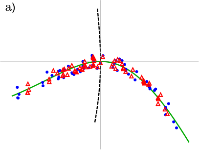
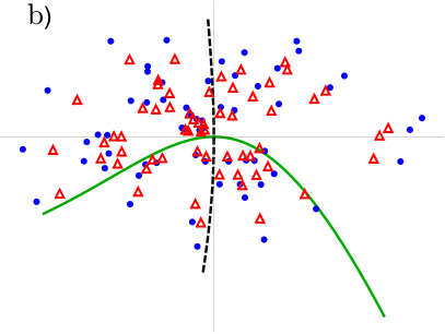
Figure 1: Two cases of data distribution. The blue dots (initial conditions) are mapped into the red triangles by the nonlinear map $\boldsymbol{F}$ given by equation (36). a) data points are distributed in the neighbourhood of the solid green curve, which is identified as an approximate invariant manifold. b) Initial conditions are well-distributed in the neighbourhood of the steady state and there is no obvious manifold structure. For completeness, the second invariant manifold is denoted by the dashed line.

Not all methods that identify low-dimensional models produce ROMs. In some cases the data lie on a low-dimensional manifold embedded in a high-dimensional, typically Euclidean, space as in figure 1(a). In this case the task is to parametrise the low-dimensional manifold and fit a model to the data in the coordinates of the parametrisation. The choice of parametrisation influences the form of the model. It is desired to use a parametrisation that yields a model with the least number of parameters. Approaches to reduce the number of parameters include compressed sensing [22, 7, 12, 13, 18] and normal form methods [49, 64, 17]. The methods to obtain a parametrisation of the manifold include diffusion maps [19], isomaps [58], autoencoders [36, 18, 33, 17] and equation-free models [34, 35].

The main focus of this paper is genuine ROMs, where we need to find structure in a cloud of data as illustrated in figure 1(b). An invariant manifold provides such structure, since all trajectories starting from the manifold stay on the manifold for all times. However an invariant manifold is not defined by the dynamics on it but by the dynamics in its neighbourhood [25, 21, 14]. This means that identifying a manifold must also involve identifying the dynamics in its neighbourhood, which is regularly omitted, such as in [17]. We find that resolving the nearby dynamics is the same as identifying an invariant foliation, as explained in section 2.2.

Invariant foliations [55] can also be used to find structure in data like in figure 1(b). An invariant foliation consists of a family of leaves (manifolds) that map onto each other under the dynamics of our system as in figure 4(a). Each leaf of the foliation has a parameter from a space which has the dimensionality of the phase space minus the dimensionality of a leaf. As the leaves map onto each other, so do the parameters, which then defines a low-dimensional map or ROM. A leaf that maps onto itself is an invariant manifold. Invariant foliations are also useful to find suitable initial conditions for ROMs [50].

A natural question is if we have exhausted all possible concepts that identify structure in dynamic data. To address this, we systematically explore how a physical (or any other data producing) system can be related to a mathematical model. This allows us to categorise ROM concepts and choose the most suitable one for a given purpose. Through this process we arrive at the definitions of four cases: invariant foliations, invariant manifolds, autoencoders and equation-free models, and uncover their relations to each other.

We find that not all methods are applicable to off-line produced data. Indeed, calculating an invariant manifold requires actively probing the mathematical model [29]. If a model is not available, the physical system must be placed under closed-loop control, such as in control-based continuation [53, 3], which can currently identify equilibria or periodic orbits, but potentially it could also be used to find invariant manifolds of those equilibria and periodic orbits. Equation-free models were developed to recover inherently low-order dynamics from large systems by systematically probing the system input [34, 35]. However, not all systems can be put under closed-loop control, mainly because either setting up the required high-speed control loop is too costly or time consuming, or the system is simply inaccessible to the data analyst. In this case, the data collection is carried out separately from the data analysis without instant feedback to the system. We call this case open-loop or off-line data collection. We conclude that invariant foliations and autoencoders can be fitted to off-line data, but only invariant foliations produce genuine ROMs.

Surprisingly, invariant foliations were not explored for ROM identification before paper [55]. Here, we propose a two-stage process, which finds an invariant foliation [55], that captures a low-order model and then finds a transverse and locally defined invariant foliation, whose fixed leaf is the invariant manifold with the same dynamics as the globally defined invariant foliation. This ensures that we take into account all data when the low-order dynamics is uncovered, and at the same time also produce a familiar structure, which is the corresponding invariant manifold. As per remark 15, this process may be simplified at the possible cost of losing some accuracy.

Another contribution of the paper is that we resolve the problem with high-dimensional data, which requires the approximation of high-dimensional functions, when invariant foliations are identified. We use polynomials that have compressed tensor coefficients [27], and whose complexity scales linearly, instead of combinatorially with the underlying dimension. Compressed tensors in the hierarchical Tucker format (HT) [28] are amenable to singular value decomposition [26], hence by calculating the singular values we can check the accuracy of the approximation. In addition, compressed tensors can be truncated if some singular values are near zero without losing their accuracy. However for our purpose, the most important property is that within an optimisation framework a HT tensor is linear in each of its parameter matrices (when the rest of the parameters are fixed), which gives us a convex cost function. Indeed, when solving the invariance equation of the foliation, we use a block coordinate descent method, the Gauss-Southwell scheme [41], which significantly speeds up the solution process. We also note that optimisation of each coefficient matrix of a HT tensor is constrained to a matrix manifold, hence we use a trust-region method designed for matrix manifolds [8, 20] when solving for individual matrix components.

A ROM is usually represented in a nonlinear coordinate system, hence the quantities predicted by the ROM may not behave the same way as in Euclidean frames. This is particularly true for instantaneous frequencies and damping ratios of decaying vibrations. In section 3 we take the distortion of the nonlinear coordinate system into account and derive correct values of instantaneous frequencies and damping ratios.

The structure of the paper is as follows. We first discuss the type of data assumed for ROM identification. Then we define what a ROM is and go through all possible connections between a data producing system and a ROM. We then classify the uncovered conceptual connections along two properties: whether they are applicable to off-line data or produce genuine ROMs. Next, we discuss instantaneous frequencies and damping ratios in nonlinear frames. In section 4 we summarise the proposed and tested numerical algorithms, and describe their implementation details. Finally, we discuss three example problems. We start with a conceptual model that illustrates the non-applicability of autoencoders to genuine model order reduction. We then use a nonlinear ten-dimensional mathematical model to create synthetic data sets. Here we demonstrate the accuracy of our method to full state-space data, but also highlight problems with phase-space reconstruction from scalar signals. Finally, we analyse vibration data from a jointed beam, for which there is no accurate physical model due to the frictional interface in the joint.

1.1 Set-up

The first step on our journey is to characterise the type of data we are working with. We assume a real $n$-dimensional Euclidean space, denoted by $X$ (a vector space with an inner product $\left\langle\cdot,\cdot\right\rangle_{X}:X\times X\to\mathbb{R}$), which contains all our data. We further assume that the data is produced by a deterministic process, which is represented by an unknown map $\boldsymbol{F}:X\to X$. In particular, the data is organised into $N\in\mathbb{N}^{+}$ pairs of vectors from space $X$, that is

$$\left(\boldsymbol{x}_{k},\boldsymbol{y}_{k}\right),\;k=1,\ldots,N$$

that satisfy

$$\boldsymbol{y}_{k}=\boldsymbol{F}\left(\boldsymbol{x}_{k}\right)+\boldsymbol{\xi}_{k},\;k=1,\ldots,N,$$ (1)

where $\boldsymbol{\xi}_{k}\in X$ represents a small measurement noise, which is sampled from a distribution with zero mean. Equation (1) describes pieces of trajectories if for some $k\in\left\{1,\ldots,N\right\}$, $\boldsymbol{x}_{k+1}=\boldsymbol{y}_{k}$. The state of the system can also be defined on a manifold, in which case $X$ is chosen such that the manifold is embedded in $X$ according to Whitney’s embedding theorem [62]. It is also possible that the state cannot be directly measured, in which case Taken’s delay embedding technique [57] can be used to reconstruct the state, which we will do subsequently in an optimal manner [16]. As a minimum, we require that our system is observable [30].

For the purpose of this paper we also assume a fixed point at the origin, such that $\boldsymbol{F}\left(\boldsymbol{0}\right)=\boldsymbol{0}$ and that the domain of $\boldsymbol{F}$ is a compact and connected subset $G\subset X$ that includes a neighbourhood of the origin.

2 Reduced order models

We now describe a weak definition of a ROM, which only requires invariance. There are two ingredients of a ROM: a function connecting vector space $X$ to another vector space $Z$ of lower dimensionality and a map on vector space $Z$. The connection can go two ways, either from $Z$ to $X$ or from $X$ to $Z$. To make this more precise, we also assume that $Z$ has an inner product $\left\langle\cdot,\cdot\right\rangle_{Z}:Z\times Z\to\mathbb{R}$ and that $\dim Z<\dim X$. The connection $\boldsymbol{U}:X\to Z$ is called an encoder and the connection $\boldsymbol{W}:Z\to X$ is called a decoder. We also assume that both the encoder and the decoder are continuously differentiable and their Jacobians have full rank. Our terminology is borrowed from computer science [36], but we can also use mathematical terms that calls $\boldsymbol{U}$ a manifold submersion [38] and $\boldsymbol{W}$ a manifold immersion [37]. In accordance with our assumption that $\boldsymbol{F}\left(\boldsymbol{0}\right)=\boldsymbol{0}$, we also assume that $\boldsymbol{U}\left(\boldsymbol{0}\right)=\boldsymbol{0}$ and $\boldsymbol{W}\left(\boldsymbol{0}\right)=\boldsymbol{0}$.

Definition 1.

Assume two maps $\boldsymbol{F}:X\to X$, $\boldsymbol{S}:Z\to Z$ and an encoder $\boldsymbol{U}:X\to Z$ or a decoder $\boldsymbol{W}:Z\to X$.

1. The encoder-map pair $\left(\boldsymbol{U},\boldsymbol{S}\right)$ is a ROM of $\boldsymbol{F}$ if for all initial conditions $\boldsymbol{x}_{0}\in G\subset X$, the trajectory $\boldsymbol{x}_{k+1}=\boldsymbol{F}\left(\boldsymbol{x}_{k}\right)$ and for initial condition $\boldsymbol{z}_{0}=\boldsymbol{U}\left(\boldsymbol{x}_{0}\right)$ the second trajectory $\boldsymbol{z}_{k+1}=\boldsymbol{S}\left(\boldsymbol{z}_{k}\right)$ are connected such that $\boldsymbol{z}_{k}=\boldsymbol{U}\left(\boldsymbol{x}_{k}\right)$ for all $k>0$.

2. The decoder-map pair $\left(\boldsymbol{W},\boldsymbol{S}\right)$ is a ROM of $\boldsymbol{F}$ if for all initial conditions $\boldsymbol{z}_{0}\in H=\left\{\boldsymbol{z}\in Z:\boldsymbol{W}\left(z\right)\in G\right\}$, the trajectory $\boldsymbol{z}_{k+1}=\boldsymbol{S}\left(\boldsymbol{z}_{k}\right)$ and for initial condition $\boldsymbol{x}_{0}=\boldsymbol{W}\left(\boldsymbol{z}_{0}\right)$ the second trajectory $\boldsymbol{x}_{k+1}=\boldsymbol{F}\left(\boldsymbol{x}_{k}\right)$ are connected such that $\boldsymbol{x}_{k}=\boldsymbol{W}\left(\boldsymbol{z}_{k}\right)$ for all $k>0$.

Remark 2.

In essence, a ROM is a model whose trajectories are connected to the trajectories of our system $\boldsymbol{F}$. We call this property invariance. It is possible to define a weaker ROM, where the connections $\boldsymbol{z}_{k}=\boldsymbol{U}\left(\boldsymbol{x}_{k}\right)$ or $\boldsymbol{x}_{k}=\boldsymbol{W}\left(\boldsymbol{z}_{k}\right)$ are only approximate, which is not discussed here.

The following corollary can be thought of as an equivalent definition of a ROM.

Corollary 3.

The encoder-map pair $\left(\boldsymbol{U},\boldsymbol{S}\right)$ or decoder-map pair $\left(\boldsymbol{W},\boldsymbol{S}\right)$ is a ROM if and only if either invariance equation

$$\boldsymbol{S}\left(\boldsymbol{U}\left(\boldsymbol{x}\right)\right) =\boldsymbol{U}\left(\boldsymbol{F}\left(\boldsymbol{x}\right)\right),\quad\boldsymbol{x}\in G\quad\text{or}$$ (2)

$$\boldsymbol{W}\left(\boldsymbol{S}\left(\boldsymbol{z}\right)\right) =\boldsymbol{F}\left(\boldsymbol{W}\left(\boldsymbol{z}\right)\right),\;\boldsymbol{z}\in H,$$ (3)

hold, where $H=\left\{\boldsymbol{z}\in Z:\boldsymbol{W}\left(z\right)\in G\right\}$.

Proof.

Let us assume that (2) holds, and choose an $\boldsymbol{x}_{0}\in X$ and let $\boldsymbol{z}_{0}=\boldsymbol{U}\left(\boldsymbol{x}_{0}\right)$. First we check whether $\boldsymbol{z}_{k}=\boldsymbol{U}\left(\boldsymbol{x}_{k}\right)$, if $\boldsymbol{x}_{k}=\boldsymbol{F}^{k}\left(\boldsymbol{x}_{0}\right)$, $\boldsymbol{z}_{k}=\boldsymbol{S}^{k}\left(\boldsymbol{z}_{0}\right)$ and (2) hold. Substituting $\boldsymbol{x}=\boldsymbol{F}^{k}\left(\boldsymbol{x}_{0}\right)$ into (2) yields

$$\boldsymbol{S}^{k}\left(\boldsymbol{z}_{0}\right) =\boldsymbol{U}\left(\boldsymbol{F}^{k}\left(\boldsymbol{x}_{0}\right)\right)$$

$$\boldsymbol{z}_{k} =\boldsymbol{U}\left(\boldsymbol{x}_{k}\right).$$

Now in reverse, assuming that $\boldsymbol{z}_{k}=\boldsymbol{U}\left(\boldsymbol{x}_{k}\right)$, $\boldsymbol{z}_{k}=\boldsymbol{S}^{k}\left(\boldsymbol{z}_{0}\right)$, $\boldsymbol{x}_{k}=\boldsymbol{F}^{k}\left(\boldsymbol{x}_{0}\right)$ and setting $k=1$ yields that

$$\boldsymbol{z}_{1}=\boldsymbol{S}\left(\boldsymbol{z}_{0}\right) =\boldsymbol{U}\left(\boldsymbol{x}_{1}\right),$$

$$\boldsymbol{S}\left(\boldsymbol{U}\left(\boldsymbol{x}_{0}\right)\right) =\boldsymbol{U}\left(\boldsymbol{F}\left(\boldsymbol{x}_{0}\right)\right),$$

which is true for all $\boldsymbol{x}_{k-1}\in G$, hence (2) holds. The proof for the decoder is identical, except that we swap $\boldsymbol{F}$ and $\boldsymbol{S}$ and replace $\boldsymbol{U}$ with $\boldsymbol{W}.$ ∎

a) b)

c) d)

Figure 2: Commutative diagrams of a) invariant foliations, b) invariant manifolds, and connection diagrams of c) autoencoders and d) equation-free models. The dashed arrows denote the chain of function composition(s) that involves $\boldsymbol{F}$, the continuous arrows denote the chain of function composition(s) that involves map $\boldsymbol{S}$. The encircled vector space denotes the domain of the invariance equation and the boxed vector space is the target of the invariance equation.

Now the question arises if we can use a combination of an encoder and a decoder? This is the case of the autoencoder or nonlinear principal component analysis [36] and the equation-free model [34, 35]. Indeed, there are four combinations of encoders and decoders, which are depicted in diagrams 2(a,b,c,d). We name these four scenarios as follows.

Definition 4.

We call the connections displayed in figures 2(a,b,c,d), invariant foliation, invariant manifold, autoencoder and equation-free model, respectively.

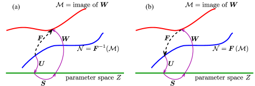
Figure 3: (a) Autoencoder. Encoder $\boldsymbol{U}$ maps data to parameter space $Z$, then the low-order map $\boldsymbol{S}$ takes the parameter forward in time and finally the decoder $\boldsymbol{W}$ brings the new parameter back to the state space. This chain of maps denoted by solid purple arrows must be the same as map $\boldsymbol{F}$ denoted by the dashed arrow. The two results can only match between two manifolds $\mathcal{M}$ and $\mathcal{N}$ and not elsewhere in the state space. Manifold $\mathcal{M}$ is invariant if and only if $\mathcal{M}\subset\mathcal{N}$, which is not guaranteed by this construction. (b) Equation-free model. The only difference from the autoencoder is the reversal of the arrow under $\boldsymbol{F}$, hence $\boldsymbol{S}\left(\boldsymbol{z}\right)=\boldsymbol{U}\left(\boldsymbol{F}\left(\boldsymbol{W}\left(\boldsymbol{z}\right)\right)\right)$.

As we walk through the dashed and solid arrows in diagram 2(a), we find the two sides of the invariance equation (2). If we do the same for diagram 2(b), we find equation (3). This implies that invariant foliations and invariant manifolds are ROMs. The same is not true for autoencoders and equation-free models. Reading off diagram 2(c), the autoencoder must satisfy

$$\boldsymbol{W}\left(\boldsymbol{S}\left(\boldsymbol{U}\left(\boldsymbol{x}\right)\right)\right)=\boldsymbol{F}\left(\boldsymbol{x}\right).$$ (4)

Equation (4) is depicted in figure 3(a). Since the decoder $\boldsymbol{W}$ maps onto a manifold $\mathcal{M}$, equation (4) can only hold if $\boldsymbol{x}$ is chosen from the preimage of $\mathcal{M}$, that is, $\boldsymbol{x}\in\mathcal{N}=\boldsymbol{F}^{-1}\left(\mathcal{M}\right)$. For invariance, we need $\boldsymbol{F}\left(\mathcal{M}\right)\subset\mathcal{M}$, which is the same as $\mathcal{M}\subset\mathcal{N}$ if $\boldsymbol{F}$ is invertible. However, the inclusion $\mathcal{M}\subset\mathcal{N}$ is not guaranteed by equation (4). The only way to guarantee $\mathcal{M}\subset\mathcal{N}$, is by stipulating that the function composition $\boldsymbol{W}\circ\boldsymbol{U}$ is the identity map on the data. A trivial case is when $\dim Z=\dim X$ or, in general, when all data fall onto a $\dim Z$ dimensional submanifold of $X$. Indeed, the standard way to find an autoencoder [36] is to solve

$$\arg\min_{\boldsymbol{U},\boldsymbol{W}}\sum_{k=1}^{N}\left\|\boldsymbol{W}\left(\boldsymbol{U}\left(\boldsymbol{x}_{k}\right)\right)-\boldsymbol{x}_{k}\right\|^{2}.$$ (5)

Unfortunately, if the data is not on a $\dim Z$ dimensional submanifold of $X$, which is the case of genuine ROMs, the minimum of $\sum_{k=1}^{N}\left\|\boldsymbol{W}\left(\boldsymbol{U}\left(\boldsymbol{x}_{k}\right)\right)-\boldsymbol{x}_{k}\right\|^{2}$ will be far from zero and the location of $\mathcal{M}$ as the solution of (5) will only indicate where the data is in the state space. It is customary to seek a solution to (5) under the normalising condition that $\boldsymbol{U}\circ\boldsymbol{W}$ is the identity and hence $\boldsymbol{S}=\boldsymbol{U}\circ\boldsymbol{F}\circ\boldsymbol{W}$.

The equation-free model in diagram 2(d) is identical to the autoencoder 2(c) if we replace $\boldsymbol{F}$ with $\boldsymbol{F}^{-1}$ and $\boldsymbol{S}$ with $\boldsymbol{S}^{-1}$. Reading off diagram 2(d), the equation-free model must satisfy

$$\boldsymbol{S}\left(\boldsymbol{z}\right)=\boldsymbol{U}\left(\boldsymbol{F}\left(\boldsymbol{W}\left(\boldsymbol{z}\right)\right)\right).$$ (6)

Equation (6) immediately provides $\boldsymbol{S}$, for any $\boldsymbol{U},$ $\boldsymbol{W}$, without identifying any structure in the data.

Only invariant foliations, through equation (2) and autoencoders through equations (4) and (5) can be fitted to off-line data. Invariant manifolds and equation-free models require the ability the manipulate the input of our system $\boldsymbol{F}$ during the identification process. Indeed, for off-line data, produced by equation (1), the foliation invariance equation (2) turns into an optimisation problem

$$\arg\min_{\boldsymbol{S},\boldsymbol{U}}\sum_{k=1}^{N}\left\|\boldsymbol{x}_{k}\right\|^{-2}\left\|\boldsymbol{S}\left(\boldsymbol{U}\left(\boldsymbol{x}_{k}\right)\right)-\boldsymbol{U}\left(\boldsymbol{y}_{k}\right)\right\|^{2},$$ (7)

and the autoencoder equation (4) turns into

$$\arg\min_{\boldsymbol{S},\boldsymbol{U},\boldsymbol{W}}\sum_{k=1}^{N}\left\|\boldsymbol{x}_{k}\right\|^{-2}\left\|\boldsymbol{W}\left(\boldsymbol{S}\left(\boldsymbol{U}\left(\boldsymbol{x}_{k}\right)\right)\right)-\boldsymbol{y}_{k}\right\|^{2}.$$ (8)

For the optimisation problem (7) to have a unique solution, we need to apply a constraint to $\boldsymbol{U}$. One possible constraint is explained in remark 7. In case of the autoencoder (8), the constraint, in addition to the one restricting $\boldsymbol{U}$, can be that $\boldsymbol{U}\circ\boldsymbol{W}$ is the identity, as also stipulated in [17].

2.1 Invariant foliations and invariant manifolds

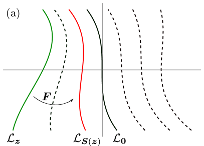
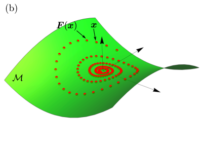
Figure 4: (a) Invariant foliation: a leaf $\mathcal{L}_{\boldsymbol{z}}$ is being mapped onto leaf $\mathcal{L}_{\boldsymbol{S}\left(\boldsymbol{z}\right)}$. Since the origin $\boldsymbol{0}\in Z$ is a steady state of $\boldsymbol{S}$, the leaf $\mathcal{L}_{\boldsymbol{0}}$ is mapped into itself and therefore it is an invariant manifold. (b) Invariant manifold: a single trajectory, represented by red dots, starting from the invariant manifold $\mathcal{M}$ remains on the green invariant manifold.

An encoder represents a family of manifolds, called foliation, which is the set of constant level surfaces of $\boldsymbol{U}$. A single level surface is called a leaf of the foliation, hence the foliation is a collection of leaves. In mathematical terms a leaf with parameter $\boldsymbol{z}\in Z$ is denoted by

$$\mathcal{L}_{\boldsymbol{z}}=\left\{\boldsymbol{x}\in G\subset X:\boldsymbol{U}\left(\boldsymbol{x}\right)=\boldsymbol{z}\right\}.$$ (9)

All leaves are $\dim X-\dim Z$ dimensional differentiable manifolds, because we assumed that the Jacobian $D\boldsymbol{U}$ has full rank [38]. The collection of all leaves is a foliation, denoted by

$$\mathcal{F}=\left\{\mathcal{L}_{\boldsymbol{z}}:\boldsymbol{z}\in H\right\},$$

where $H=\boldsymbol{U}\left(G\right)$. The foliation is characterised by its co-dimension, which is the same as $\dim Z$. Invariance equation (2) means that each leaf of the foliation is mapped onto another leaf, in particular the leaf with parameter $\boldsymbol{z}$ is mapped onto the leaf with parameter $\boldsymbol{S}\left(\boldsymbol{z}\right)$, that is

$$\boldsymbol{F}\left(\mathcal{L}_{\boldsymbol{z}}\right)\subset\mathcal{L}_{\boldsymbol{S}\left(\boldsymbol{z}\right)}.$$

Due to our assumptions, leaf $\mathcal{L}_{\boldsymbol{0}}$ is an invariant manifold, because $\boldsymbol{F}\left(\mathcal{L}_{\boldsymbol{0}}\right)\subset\mathcal{L}_{\boldsymbol{0}}$. This geometry is illustrated in figure 4(a).

We now characterise the existence and uniqueness of invariant foliations about a fixed point. We assume that $\boldsymbol{F}$ is a $C^{r}$, $r\geq 2$ map and that the Jacobian matrix $D\boldsymbol{F}\left(\boldsymbol{0}\right)$ has eigenvalues $\mu_{1},\ldots,\mu_{n}$ such that $\left|\mu_{i}\right|<1$, $i=1,\ldots,n$. To select the invariant manifold or foliation we assume two $\nu$-dimensional linear subspaces $E$ of $X$ and $E^{\star}$ of $X$ corresponding to eigenvalues $\mu_{1},\ldots,\mu_{\nu}$ such that $D\boldsymbol{F}\left(\boldsymbol{0}\right)E\subset E$ and for the adjoint map $\left(D\boldsymbol{F}\left(\boldsymbol{0}\right)\right)^{\star}E^{\star}\subset E^{\star}$.

Definition 5.

The number

$$\beth_{E^{\star}}=\frac{\min_{k=1\ldots\nu}\log\left|\mu_{k}\right|}{\max_{k=1\ldots n}\log\left|\mu_{k}\right|}$$

is called the spectral quotient of the left-invariant linear subspace $E^{\star}$ of $\boldsymbol{F}$ about the origin.

Theorem 6.

Assume that $D\boldsymbol{F}\left(\boldsymbol{0}\right)$ is semisimple and that there exists an integer $\sigma\geq 2$, such that $\beth_{E^{\star}}<\sigma\leq r$. Also assume that

$$\prod_{k=1}^{n}\mu_{k}^{m_{k}}\neq\mu_{j},\;j=1,\ldots,\nu$$ (10)

for all $m_{k}\geq 0$, $1\leq k\leq n$ with at least one $m_{l}\neq 0$, $\nu+1\leq l\leq n$ and with $\sum_{k=0}^{n}m_{k}\leq\sigma-1$. Then in a sufficiently small neighbourhood of the origin there exists an invariant foliation $\mathcal{F}$ tangent to the left-invariant linear subspace $E^{\star}$ of the $C^{r}$ map $\boldsymbol{F}$. The foliation $\mathcal{F}$ is unique among the $\sigma$ times differentiable foliations and it is also $C^{r}$ smooth.

Proof.

The proof is carried out in [55]. Note that the assumption of $D\boldsymbol{F}\left(\boldsymbol{0}\right)$ being semisimple was used to simplify the proof in [55], therefore it is unlikely to be needed. ∎

Remark 7.

Theorem 6 only concerns the uniqueness of the foliation, but not the encoder $\boldsymbol{U}$. However, for any smooth and invertible map $\boldsymbol{R}:Z\to Z$, the encoder $\tilde{\boldsymbol{U}}=\boldsymbol{R}\circ\boldsymbol{U}$ represents the same foliation and the nonlinear map $\boldsymbol{S}$ transforms into $\tilde{\boldsymbol{S}}=\boldsymbol{R}\circ\boldsymbol{S}\circ\boldsymbol{R}^{-1}$. If we want to solve the invariance equation (2), we need to constrain $\boldsymbol{U}$. The simplest such constraint is that

$$\boldsymbol{U}\left(\boldsymbol{W}_{1}\boldsymbol{z}\right)=\boldsymbol{z},$$ (11)

where $\boldsymbol{W}_{1}:Z\to X$ is a linear map with full rank such that $E^{\star}\cap\ker\boldsymbol{W}_{1}^{\star}=\left\{\boldsymbol{0}\right\}$. To explain the meaning of equation (11), we note that the image of $\boldsymbol{W}_{1}$ is a linear subspace $\mathcal{H}$ of $X$. Equation (11) therefore means that each leaf $\mathcal{L}_{\boldsymbol{z}}$ must intersect subspace $\mathcal{H}$ exactly at parameter $\boldsymbol{z}$. The condition $E^{\star}\cap\ker\boldsymbol{W}_{1}^{\star}=\left\{\boldsymbol{0}\right\}$ then means that the leaf $\mathcal{L}_{\boldsymbol{0}}$ has a transverse intersection with subspace $\mathcal{H}$. This is similar to the graph-style parametrisation of a manifold over a linear subspace.

Remark 8.

Eigenvalues and eigenfunctions of the Koopman operator [39, 40] are invariant foliations. Indeed, the Koopman operator is defined as $\left(\mathcal{K}\boldsymbol{u}\right)\left(\boldsymbol{x}\right)=\boldsymbol{u}\left(\boldsymbol{F}\left(\boldsymbol{x}\right)\right)$. If we assume that $\boldsymbol{U}=\left(\boldsymbol{u}_{1},\ldots,\boldsymbol{u}_{\nu}\right)$ is a collection of functions $\boldsymbol{u}_{j}:X\to\mathbb{R}$, $Z=\mathbb{R}^{\nu}$, then $\boldsymbol{U}$ spans an invariant subspace of $\mathcal{K}$ if there exists a linear map $\boldsymbol{S}$ such that $\mathcal{K}\left(\boldsymbol{U}\right)=\boldsymbol{S}\boldsymbol{U}$. Expanding this equation yields $\boldsymbol{U}\left(\boldsymbol{F}\left(\boldsymbol{x}\right)\right)=\boldsymbol{S}\boldsymbol{U}\left(\boldsymbol{x}\right)$, which is the same as the invariance equation (2), except that $\boldsymbol{S}$ is linear. The existence of linear map $\boldsymbol{S}$ requires further non-resonance conditions, which are

$$\prod_{k=1}^{\nu}\mu_{k}^{m_{k}}\neq\mu_{j},\;j=1,\ldots,\nu$$ (12)

for all $m_{k}\geq 0$ such that $\sum_{k=0}^{n}m_{k}\leq\sigma-1$. Equation (12) is referred to as the set of internal non-resonance conditions, because these are intrinsic to the invariant subspace $E^{\star}$. In many cases $\boldsymbol{S}$ represents the slowest dynamics, hence even if there are no internal resonances, the two sides of (12) will be close to each other for some set of $m_{1},\ldots,m_{\nu}$ exponents and that causes numerical issues leading to undesired inaccuracies. We will illustrate this in section 5.2.

Now we discuss invariant manifolds. A decoder $\boldsymbol{W}$ defines a differentiable manifold

$$\mathcal{M}=\left\{\boldsymbol{W}\left(\boldsymbol{z}\right):\boldsymbol{z}\in H\right\},$$

where $H=\left\{\boldsymbol{z}\in Z:\boldsymbol{W}\left(\boldsymbol{z}\right)\in G\right\}$. Invariance equation (3) is equivalent to the geometric condition that $\boldsymbol{F}\left(\mathcal{M}\right)\subset\mathcal{M}$. This geometry is shown in figure 4(b), which illustrates that if a trajectory is started on $\mathcal{M}$, all subsequent points of the trajectory stay on $\mathcal{M}$.

Invariant manifolds as a concept cannot be used to identify ROMs from off-line data. As we will see below, invariant manifolds can still be identified as a leaf of an invariant foliation, but not through the invariance equation (3). Indeed, it is not possible to guess the manifold parameter $\boldsymbol{z}\in Z$ from data. Introducing an encoder $\boldsymbol{U}:X\to Z$ to calculate $\boldsymbol{z}=\boldsymbol{U}\left(\boldsymbol{x}\right)$, transforms the invariant manifold into an autoencoder, which does not guarantee invariance.

We now state the conditions of the existence and uniqueness of an invariant manifold.

Definition 9.

The number

$$\aleph_{E}=\frac{\min_{k=\nu+1\ldots n}\log\left|\mu_{k}\right|}{\max_{k=1\ldots\nu}\log\left|\mu_{k}\right|}$$

is called the spectral quotient of the right-invariant linear subspace $E$ of map $\boldsymbol{F}$ about the origin.

Theorem 10.

Assume that there exists an integer $\sigma\geq 2$, such that $\aleph_{E}<\sigma\leq r$. Also assume that

$$\prod_{k=1}^{\nu}\mu_{k}^{m_{k}}\neq\mu_{j},\;j=\nu+1,\ldots,n$$ (13)

for all $m_{k}\geq 0$ such that $\sum_{k=0}^{\nu}m_{k}\leq\sigma-1$. Then in a sufficiently small neighbourhood of the origin there exists an invariant manifold $\mathcal{\mathcal{M}}$ tangent to the invariant linear subspace $E$ of the $C^{r}$ map $\boldsymbol{F}$. The manifold $\mathcal{M}$ is unique among the $\sigma$-times differentiable manifolds and it is also $C^{r}$ smooth.

Proof.

The theorem is a subset of theorem 1.1 in [14]. ∎

Remark 11.

To calculate an invariant manifold with a unique representation, we need to impose a constraint on $\boldsymbol{W}$ and/or $\boldsymbol{S}$. The simplest constraint is imposed by

$$\boldsymbol{U}_{1}\boldsymbol{W}\left(\boldsymbol{z}\right)=\boldsymbol{z},$$ (14)

where $\boldsymbol{U}_{1}:Z\to X$ is a linear map with full rank such that $E\cap\ker\boldsymbol{U}_{1}^{\star}=\left\{\boldsymbol{0}\right\}$. This is similar to a graph-style parametrisation (akin to theorem 1.2 in [14]), where the range of $\boldsymbol{U}_{1}$ must span the linear subspace $E$. Constraint (14) can break down for large $\left\|\boldsymbol{z}\right\|$, when $\boldsymbol{U}_{1}D\boldsymbol{W}\left(\boldsymbol{z}\right)$ does not have full rank. A globally suitable constraint is that $D\boldsymbol{W}^{\star}\left(\boldsymbol{z}\right)D\boldsymbol{W}\left(\boldsymbol{z}\right)=\boldsymbol{I}$.

For linear subspaces $E$ and $E^{\star}$ with eigenvalues closest to the complex unit circle (representing the slowest dynamics), $\beth_{E}=1$ and $\aleph_{E}$ is maximal. Therefore the foliation corresponding to the slowest dynamics requires the least smoothness, while the invariant manifold requires the maximum smoothness for uniqueness.

Table 1 summarises the main properties of the three conceptually different model identification techniques. Ultimately, in the presence of off-line data, only invariant foliations can be fitted to the data and produce a ROM at the same time.

	Invariant foliation	Invariant manifold	Autoencoder	Eq.-free model
Usable closed-loop	YES	YES	YES	YES
Usable open-loop	YES	NO	YES	NO
Obtains a ROM	YES	YES	NO	NO
Uniqueness	slowest most unique	slowest least unique	NO	NO
References	[55, 39, 50, 51]	[52, 21, 14, 15, 29, 56, 61]	[17, 18, 33]	[34, 35]

Table 1: Comparison of invariant foliations, invariant manifolds and autoencoders.

2.2 Invariant manifolds represented by locally defined invariant foliations

As discussed before, we cannot fit invariant manifolds to data, instead we can fit an invariant foliation that contains our invariant manifold (which is the leaf containing the fixed point $\mathcal{L}_{\boldsymbol{0}}$ at the origin). This invariant foliation only needs to be defined near the invariant manifold and therefore we can simplify the functional representation of the encoder that defines the foliation. In this section we discuss this simplification.

To begin with, assume that we already have an invariant foliation $\mathcal{F}$ with an encoder $\boldsymbol{U}$ and nonlinear map $\boldsymbol{S}$. Our objective is to find the invariant manifold $\mathcal{M}$, represented by decoder $\boldsymbol{W}$ that has the same dynamics $\boldsymbol{S}$ as the foliation. This is useful if we want to know quantities that are only defined for invariant manifolds, such as instantaneous frequencies and damping ratios. Formally, we are looking for a simplified invariant foliation $\hat{\mathcal{F}}$ with encoder $\hat{\boldsymbol{U}}:X\to\hat{Z}$ that together with $\mathcal{F}$ form a coordinate system in $X$. (Technically speaking, $\left(\boldsymbol{U},\hat{\boldsymbol{U}}\right):X\to Z\times\hat{Z}$ must be a isomorphism.) In this case our invariant manifold is the zero level surface of encoder $\hat{\boldsymbol{U}}$, i.e., $\mathcal{M}=\hat{\mathcal{L}}_{0}\in\hat{\mathcal{F}}$. Naturally, we must have $\dim Z+\dim\hat{Z}=\dim X$.

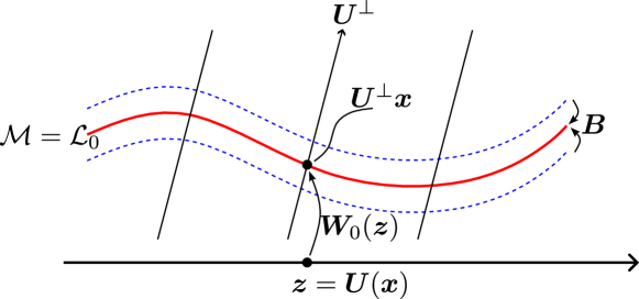
Figure 5: Approximate invariant foliation. The linear map $\boldsymbol{U}^{\perp}$ and the nonlinear map $\boldsymbol{U}$ create a coordinate system, so that in this frame the invariant manifold $\mathcal{M}$ is given by $\boldsymbol{U}^{\perp}\boldsymbol{x}=\boldsymbol{W}_{\boldsymbol{0}}\left(\boldsymbol{z}\right)$, where $\boldsymbol{z}=\boldsymbol{U}\left(\boldsymbol{z}\right)$. We then allow to shift manifold $\mathcal{M}$ in the $\boldsymbol{U}^{\perp}$ direction such that $\boldsymbol{U}^{\perp}\boldsymbol{x}-\boldsymbol{W}_{\boldsymbol{0}}\left(\boldsymbol{z}\right)=\hat{\boldsymbol{z}}$, which creates a foliation parametrised by $\hat{\boldsymbol{z}}\in\hat{Z}$. If this foliation satisfies the invariance equation in a neighbourhood of $\mathcal{M}$ with a linear map $\boldsymbol{B}$ as per equation (16), then $\mathcal{M}$ is an invariant manifold. In other words, nearby blue dashed leaves are mapped towards $\mathcal{M}$ by linear map $\boldsymbol{B}$ the same way as the underlying dynamics does.

The sufficient condition that $\mathcal{F}$ and $\hat{\mathcal{F}}$ form a coordinate system locally about the fixed point is that the square matrix

$$\boldsymbol{Q}=\begin{pmatrix}D\boldsymbol{U}\left(\boldsymbol{0}\right)\\ D\hat{\boldsymbol{U}}\left(\boldsymbol{0}\right)\end{pmatrix}$$

is invertible. Let us represent our approximate (or locally defined) encoder by

$$\hat{\boldsymbol{U}}\left(\boldsymbol{x}\right)=\boldsymbol{U}^{\perp}\boldsymbol{x}-\boldsymbol{W}_{0}\left(\boldsymbol{U}\left(\boldsymbol{x}\right)\right),$$ (15)

where $\boldsymbol{W}_{0}:Z\to\hat{Z}$ is a nonlinear map with $D\boldsymbol{W}_{0}\left(\boldsymbol{0}\right)=\boldsymbol{0}$, $\boldsymbol{U}^{\perp}:X\to\hat{Z}$ is an orthogonal linear map, $\boldsymbol{U}^{\perp}\left(\boldsymbol{U}^{\perp}\right)^{\star}=\boldsymbol{I}$ and $\boldsymbol{U}^{\perp}\boldsymbol{W}_{0}\left(\boldsymbol{z}\right)=\boldsymbol{0}$. Here, the linear map $\boldsymbol{U^{\perp}}$ measures coordinates in a transversal direction to the manifold and $\boldsymbol{W}_{0}$ prescribes where the actual manifold is along this transversal direction, while $\boldsymbol{U}$ provides the parametrisation of the manifold. All other leaves of the approximate foliation $\hat{\mathcal{F}}$ are shifted copies of $\mathcal{M}$ along the $\boldsymbol{U}^{\perp}$ direction as displayed in figure 5. A locally defined foliation means that $\hat{\boldsymbol{z}}=\hat{\boldsymbol{U}}\left(\boldsymbol{x}\right)\in\hat{Z}$ is assumed to be small, hence we can also assume linear dynamics among the leaves of $\hat{\mathcal{F}}$, which is represented by a linear operator $\boldsymbol{B}:\hat{Z}\to\hat{Z}$. Therefore the invariance equation (2) becomes

$$\boldsymbol{B}\hat{\boldsymbol{U}}\left(\boldsymbol{x}\right)=\hat{\boldsymbol{U}}\left(\boldsymbol{F}\left(\boldsymbol{x}\right)\right).$$ (16)

Once $\boldsymbol{B}$, $\boldsymbol{U}^{\perp}$ and $\boldsymbol{W}_{0}$ are found, the final step is to reconstruct the decoder $\boldsymbol{W}$ of our invariant manifold $\mathcal{M}$.

Proposition 12.

The decoder $\boldsymbol{W}$ of the invariant manifold $\mathcal{M}=\left\{\boldsymbol{x}\in X:\hat{\boldsymbol{U}}\left(\boldsymbol{x}\right)=\boldsymbol{0}\right\}$ is the unique solution of the system of equations

$$\left.\begin{array}[]{rl}\boldsymbol{U}\left(\boldsymbol{W}\left(\boldsymbol{z}\right)\right)&=\boldsymbol{z}\\ \boldsymbol{U}^{\perp}\boldsymbol{W}\left(\boldsymbol{z}\right)&=\boldsymbol{W}_{0}\left(\boldsymbol{z}\right)\end{array}\right\}.$$ (17)

Proof.

First we show that conditions (17) imply $\hat{\boldsymbol{U}}\left(\boldsymbol{W}\left(\boldsymbol{x}\right)\right)=\boldsymbol{0}$. We expand our expression using (15) into $\hat{\boldsymbol{U}}\left(\boldsymbol{W}\left(\boldsymbol{x}\right)\right)=\boldsymbol{U}^{\perp}\boldsymbol{W}\left(\boldsymbol{z}\right)-\boldsymbol{W}_{0}\left(\boldsymbol{U}\left(\boldsymbol{W}\left(\boldsymbol{z}\right)\right)\right)$, then use equations (17), which yields $\hat{\boldsymbol{U}}\left(\boldsymbol{W}\left(\boldsymbol{x}\right)\right)=\boldsymbol{0}$. To solve equations (17) for $\boldsymbol{W}$, we decompose $\boldsymbol{U}$, $\boldsymbol{W}$ into linear and nonlinear components, such that $\boldsymbol{U}\left(\boldsymbol{x}\right)=D\boldsymbol{U}\left(0\right)\boldsymbol{x}+\widetilde{\boldsymbol{U}}\left(\boldsymbol{x}\right)$ and $\boldsymbol{W}\left(\boldsymbol{z}\right)=D\boldsymbol{W}\left(0\right)\boldsymbol{z}+\widetilde{\boldsymbol{W}}\left(\boldsymbol{z}\right)$. Expanding equation (17) with the decomposed $\boldsymbol{U}$, $\boldsymbol{W}$ yields

$$\left.\begin{array}[]{rl}D\boldsymbol{U}\left(0\right)\left(D\boldsymbol{W}\left(0\right)\boldsymbol{z}+\widetilde{\boldsymbol{W}}\left(\boldsymbol{z}\right)\right)+\widetilde{\boldsymbol{U}}\left(D\boldsymbol{W}\left(0\right)\boldsymbol{z}+\widetilde{\boldsymbol{W}}\left(\boldsymbol{z}\right)\right)&=\boldsymbol{z}\\ \boldsymbol{U}^{\perp}\left(D\boldsymbol{W}\left(0\right)\boldsymbol{z}+\widetilde{\boldsymbol{W}}\left(\boldsymbol{z}\right)\right)&=\boldsymbol{W}_{0}\left(\boldsymbol{z}\right)\end{array}\right\}.$$ (18)

The linear part of equation (18) is

$$\boldsymbol{Q}D\boldsymbol{W}\left(0\right)=\begin{pmatrix}\boldsymbol{I}\\ \boldsymbol{0}\end{pmatrix},$$

hence $D\boldsymbol{W}\left(0\right)=\boldsymbol{Q}^{-1}\begin{pmatrix}\boldsymbol{I}\\ \boldsymbol{0}\end{pmatrix}$. The nonlinear part of (18) is

$$\boldsymbol{Q}\widetilde{\boldsymbol{W}}\left(\boldsymbol{z}\right)=\begin{pmatrix}-\widetilde{\boldsymbol{U}}\left(D\boldsymbol{W}\left(0\right)\boldsymbol{z}+\widetilde{\boldsymbol{W}}\left(\boldsymbol{z}\right)\right)\\ \boldsymbol{W}_{0}\left(\boldsymbol{z}\right)\end{pmatrix},$$

which can be solved by the iteration

$$\widetilde{\boldsymbol{W}}_{k+1}\left(\boldsymbol{z}\right)=\boldsymbol{Q}^{-1}\begin{pmatrix}-\widetilde{\boldsymbol{U}}\left(D\boldsymbol{W}\left(0\right)\boldsymbol{z}+\widetilde{\boldsymbol{W}}_{k}\left(\boldsymbol{z}\right)\right)\\ \boldsymbol{W}_{0}\left(\boldsymbol{z}\right)\end{pmatrix},\;\widetilde{\boldsymbol{W}}_{1}\left(\boldsymbol{z}\right)=\boldsymbol{0},\;k=1,2,\ldots.$$ (19)

Iteration (19) converges for $\left|\boldsymbol{z}\right|$ sufficiently small, due to $\widetilde{\boldsymbol{U}}$$\left(\boldsymbol{x}\right)=\mathcal{O}\left(\left|\boldsymbol{x}\right|^{2}\right)$ and $\boldsymbol{W}_{0}\left(\boldsymbol{z}\right)=\mathcal{O}\left(\left|\boldsymbol{z}\right|^{2}\right)$. ∎

As we will see in section 5, this approach provides better results than using an autoencoder. Here we have resolved the dynamics transversal to the invariant manifold $\mathcal{M}$ up to linear order. It is essential to resolve this dynamics to find invariance, not just the location of data points.

Remark 13.

More consideration is needed in case $\hat{\boldsymbol{U}}\left(\boldsymbol{x}_{k}\right)$ assumes large values over some data points. This either requires to replace $\boldsymbol{B}$ with a nonlinear map or we need to filter out data points that are not in a small neighbourhood of the invariant manifold $\mathcal{M}$. Due to $\boldsymbol{B}$ being high-dimensional, replacing it with a nonlinear map leads to numerical difficulties. Filtering data is easier. For example, we can assign weights to each term in our optimisation problem (7) depending on how far a data point is from the predicted manifold, which is the zero level surface of $\hat{\boldsymbol{U}}$. This can be done using the optimisation problem

$$\arg\min_{\boldsymbol{B},\boldsymbol{U}^{\perp},\boldsymbol{W}_{0}}\sum_{k=1}^{N}\left\|\boldsymbol{x}_{k}\right\|^{-2}\phi_{\kappa}\left(\left\|\hat{\boldsymbol{U}}\left(\boldsymbol{x}_{k}\right)\right\|^{2}\right)\left\|\boldsymbol{B}\hat{\boldsymbol{U}}\left(\boldsymbol{x}_{k}\right)-\hat{\boldsymbol{U}}\left(\boldsymbol{y}_{k}\right)\right\|^{2},$$ (20)

where

$$\phi_{\kappa}\left(x\right)=\begin{cases}\exp\frac{x}{x-\kappa^{2}}&0\leq x<\kappa^{2}\\ 0&x\geq\kappa^{2}\end{cases}$$

is the bump function and $\kappa>0$ determines the size of the neighbourhood of the invariant manifold $\mathcal{M}$ that we take into account.

Remark 14.

The approximation (16) can be made more accurate if we allow matrix $\boldsymbol{U}^{\perp}$ to vary with the parameter of the manifold $\boldsymbol{z}=\boldsymbol{U}\left(\boldsymbol{x}\right)$. In this case the encoder becomes

$$\breve{\boldsymbol{U}}\left(\boldsymbol{x}\right)=\boldsymbol{U}^{\perp}\left(\boldsymbol{U}\left(\boldsymbol{x}\right)\right)\boldsymbol{x}-\boldsymbol{W}_{0}\left(\boldsymbol{U}\left(\boldsymbol{x}\right)\right).$$

This does increase computational costs, but not nearly as much as if we were calculating a globally accurate invariant foliation. For our example problems, we find that this extension is not necessary.

Remark 15.

It is also possible to eliminate a-priori calculation of $\boldsymbol{U}$. We can assume that $\boldsymbol{U}$ is a linear map, such that $\boldsymbol{U}\boldsymbol{U}^{\star}=\boldsymbol{I}$ and treat it as an unknown in representation (15). The assumption that $\boldsymbol{U}$ is linear makes sense if we limit ourselves to a small neighbourhood of the invariant manifold $\mathcal{M}$ by setting $\kappa<\infty$ in (20), as we have already assumed a linear dynamics among the leaves of the associated foliation $\hat{\mathcal{F}}$ given by linear map $\boldsymbol{B}$. Once $\boldsymbol{B}$, $\boldsymbol{U},$ $\boldsymbol{U}^{\perp}$ and $\boldsymbol{W}_{0}$ are found, map $\boldsymbol{S}$ can also be fitted to the invariance equation (2). The equation to fit $\boldsymbol{S}$ to data is

$$\arg\min_{\boldsymbol{S}}\sum_{k=1}^{N}\left\|\boldsymbol{x}_{k}\right\|^{-2}\phi_{\kappa}\left(\left\|\hat{\boldsymbol{U}}\left(\boldsymbol{x}_{k}\right)\right\|^{2}\right)\left\|\boldsymbol{U}\boldsymbol{y}_{k}-\boldsymbol{S}\left(\boldsymbol{U}\boldsymbol{x}_{k}\right)\right\|^{2},$$

which is a straightforward linear least squares problem, if $\boldsymbol{S}$ is linear in its parameters. This approach will be further explored elsewhere.

3 Instantaneous frequencies and damping ratios

Instantaneous damping ratios and frequencies are usually defined with respect to a model that is fitted to data [32]. Here we take a similar approach and stress that these quantities only make sense in an Euclidean frame and not in the nonlinear frame of an invariant manifold or foliation. The geometry of a manifold or foliation depends on an arbitrary parametrisation, hence uncorrected results are not unique. Many studies mistakenly use nonlinear coordinate systems, for example one by the present author [56] and colleagues [10, 48]. Such calculations are only asymptotically accurate near the equilibrium. Here we describe how to correct this error.

We assume a two-dimensional invariant manifold $\mathcal{M}$, parametrised by a decoder $\boldsymbol{W}$ in polar coordinates $r,\theta$. The invariance equation (3) for the decoder $\boldsymbol{W}$ can be written as

$$\boldsymbol{W}\left(R\left(r\right),\theta+T\left(r\right)\right)=\boldsymbol{F}\left(\boldsymbol{W}\left(r,\theta\right)\right).$$ (21)

Without much thinking, (as described in [56, 55]), the instantaneous frequency and damping could be calculated as

$$\omega\left(r\right) =T\left(r\right) \left[\text{rad}/\text{step}\right],$$ (22)

$$\zeta\left(r\right) =-\frac{\log\frac{R\left(r\right)}{r}}{\omega\left(r\right)} \left[-\right],$$ (23)

respectively. The instantaneous amplitude is a norm $A\left(r\right)=\left\|\boldsymbol{W}\left(r,\cdot\right)\right\|_{A}$, for example

$$\left\|\boldsymbol{f}\right\|_{A}=\sqrt{\left\langle\boldsymbol{f},\boldsymbol{f}\right\rangle_{A}},\;\left\langle\boldsymbol{f},\boldsymbol{f}\right\rangle_{A}=\frac{1}{2\pi}\int_{0}^{2\pi}\left\langle\boldsymbol{f}\left(\theta\right),\boldsymbol{f}\left(\theta\right)\right\rangle_{X}\mathrm{d}\theta,$$ (24)

where $\left\langle\cdot,\cdot\right\rangle_{X}$ is the inner product on vector space $X$.

The frequency and damping ratio values are only accurate if there is a linear relation between $\left\|\boldsymbol{W}\left(r,\cdot\right)\right\|_{A}$ and $r$, for example

$$\left\|\boldsymbol{W}\left(r,\cdot\right)\right\|_{A}=r$$ (25)

and the relative phase between two closed curves satisfies

$$\arg\min_{\gamma}\left\|\boldsymbol{W}\left(r_{1},\cdot\right)-\boldsymbol{W}\left(r_{2},\cdot+\gamma\right)\right\|_{A}=0.$$ (26)

Equation (25) means that the instantaneous amplitude of the trajectories on manifold $\mathcal{M}$ is the same as parameter $r$, hence the map $r\mapsto R\left(r\right)$ determines the change in amplitude. Equation (26) stipulates that the parametrisation in the angular variable is such that there is no phase shift between the closed curves $\boldsymbol{W}\left(r_{1},\cdot\right)$ and $\boldsymbol{W}\left(r_{2},\cdot\right)$ for $r_{1}\neq r_{2}$. If there would be a phase shift $\gamma$, a trajectory that within a period moves from amplitude $r_{1}$ to $r_{2}$, would misrepresent its instantaneous period of vibration by phase $\gamma$, hence the frequency given by $T\left(r\right)$ would be inaccurate. In fact, one can set a continuous phase shift $\gamma\left(r\right)$ among the closed curves $\boldsymbol{W}\left(r,\cdot\right)$, such that the frequency given by $T\left(r\right)$ has a prescribed value. The following result provides accurate values for instantaneous frequencies and damping ratios.

Proposition 16.

Assume a decoder $\boldsymbol{W}:\left[0,r_{1}\right]\times\left[0,2\pi\right]\to X$ and functions $R,T:\left[0,r_{1}\right]\to\mathbb{R}$ such that they satisfy invariance equation (21).

1. A new parametrisation $\tilde{\boldsymbol{W}}$ of the manifold generated by $\boldsymbol{W}$ that satisfies the constraints (25) and (26) is given by

   $$\tilde{\boldsymbol{W}}\left(r,\theta\right)=\boldsymbol{W}\left(t,\theta+\gamma\left(t\right)\right),\;t=\kappa^{-1}\left(r\right),$$

   where

   $$\gamma\left(r\right) =-\int_{0}^{r}\frac{\int_{0}^{2\pi}\left\langle D_{1}\boldsymbol{W}\left(\rho,\theta\right),D_{2}\boldsymbol{W}\left(\rho,\theta\right)\right\rangle_{X}\mathrm{d}\theta}{\int_{0}^{2\pi}\left\langle D_{2}\boldsymbol{W}\left(\rho,\theta\right),D_{2}\boldsymbol{W}\left(\rho,\theta\right)\right\rangle_{X}\mathrm{d}\theta}\mathrm{d}\rho,$$ (27)

   $$\kappa\left(r\right) =\sqrt{\frac{1}{2\pi}\int_{0}^{2\pi}\left\langle\boldsymbol{W}\left(r,\theta\right),\boldsymbol{W}\left(r,\theta\right)\right\rangle_{X}\mathrm{d}\theta}$$ (28)

   and $\left\langle\cdot,\cdot\right\rangle_{X}$ is the inner product on vector space $X$.

2. The instantaneous natural frequency and damping ratio are calculated as

   $$\omega\left(r\right) =T\left(t\right)+\gamma\left(t\right)-\gamma\left(R\left(t\right)\right) \left[\text{rad}/\text{step}\right],$$ (29)

   $$\zeta\left(r\right) =-\frac{\log\left[r^{-1}\kappa\left(R\left(t\right)\right)\right]}{\omega\left(r\right)} \left[-\right].$$ (30)

   where $t=\kappa^{-1}\left(r\right)$.

Proof.

A proof is given in appendix C. ∎

Remark 17.

The transformed expressions (29), (30) for the instantaneous frequency and damping ratio show that any instantaneous frequency can be achieved for all $r>0$ if $R\left(r\right)\neq r$ by choosing appropriate functions $\rho,\gamma$. For example, zero frequency is achieved by solving

$$\gamma\left(r\right) =\gamma\left(R\left(r\right)\right)-T\left(r\right),$$ (31)

which is a functional equation. For an $\epsilon>0$, fix $\gamma\left(R\left(\epsilon\right)\right)=0$, $\gamma\left(\epsilon\right)=T\left(\epsilon\right)$ and some interpolating values in the interior of the interval $\left[R\left(\epsilon\right),\epsilon\right]$, then use contraction mapping to arrive at a unique solution for function $\gamma$.

Remark 18.

The same calculation applies to vector fields, $\dot{\boldsymbol{x}}=\boldsymbol{f}\left(\boldsymbol{x}\right)$, but the final result is somewhat different. Assume a decoder $\boldsymbol{W}:\left[0,r_{1}\right]\times\left[0,2\pi\right]\to X$ and functions $R,T:\left[0,r_{1}\right]\to\mathbb{R}$ such that they satisfy the invariance equation

$$D_{1}\boldsymbol{W}\left(r,\theta\right)R\left(r\right)+D_{2}\boldsymbol{W}\left(r,\theta\right)T\left(r\right)=\boldsymbol{f}\left(\boldsymbol{W}\left(r,\theta\right)\right).$$ (32)

The instantaneous natural frequency and damping ratio is calculated by

$$\omega\left(r\right) =T\left(t\right)-\dot{\gamma}\left(t\right)R\left(t\right) \left[\text{rad}/\text{unit time}\right],$$

$$\zeta\left(r\right) =-\frac{\dot{\kappa}\left(t\right)R\left(t\right)}{r\omega\left(r\right)} \left[-\right],$$

where $t=\kappa^{-1}\left(r\right)$. All other quantities are as in proposition 16. A proof is given in appendix C.

Remark 19.

Note that proposition 16 also applies if we create a different measure of amplitude, for example $\hat{\boldsymbol{W}}\left(r,\theta\right)=\boldsymbol{w}^{\star}\cdot\boldsymbol{W}\left(r,\theta\right)$, where $\boldsymbol{w}^{\star}$ is a linear map. Indeed, in the proof we did not use that $\boldsymbol{W}$ is a manifold immersion, it only served as Euclidean coordinates of points on the invariant manifold. Hence, the transformed function $\hat{\boldsymbol{W}}$ gives us the same frequencies and damping ratios as $\boldsymbol{W}$, but at linearly scaled amplitudes.

The following example illustrates that if a system is linear in a nonlinear coordinate system, we can recover the actual instantaneous damping ratios and frequencies using proposition 16. This is the case of Koopman eigenfunctions (as in remark 8), or normal form transformations where all the nonlinear terms are eliminated.

Example 20.

Let us consider the linear map

$$\begin{array}[]{rl}r_{k+1}&=\mathrm{e}^{\zeta_{0}\omega_{0}}r_{k}\\ \theta_{k+1}&=\theta_{k}+\omega_{0}\end{array}$$ (33)

and the corresponding nonlinear decoder

$$\boldsymbol{W}\left(r,\theta\right)=\left(\begin{array}[]{c}r\cos\theta-\frac{1}{4}r^{3}\cos^{3}\theta\\ r\sin\theta+\frac{1}{2}r^{3}\cos^{3}\theta\end{array}\right).$$ (34)

In terms of the polar invariance equation (21) the linear map (33) translates to $T\left(r\right)=\omega_{0}$ and $R\left(r\right)=\mathrm{e}^{\zeta_{0}\omega_{0}}r$. If we disregard the nonlinearity of $\boldsymbol{W}$, the instantaneous frequency and the instantaneous damping ratio of our hypothetical system would be constant, that is $\omega\left(r\right)=\omega_{0}$ and $\zeta\left(r\right)=\zeta_{0}$. Using proposition 16, we calculate the effect of $\boldsymbol{W}$, and find that

$$\gamma\left(r\right) =-\frac{2}{\sqrt{19}}\left(\tan^{-1}\left(\frac{15r^{2}-8}{8\sqrt{19}}\right)+\cot^{-1}\left(\sqrt{19}\right)\right),$$

$$\kappa\left(r\right) =r^{2}-\frac{3r^{4}}{16}+\frac{25r^{6}}{256}.$$

Finally, we plot expressions (29) and (30) in figure 6(a) and 6(b), respectively. It can be seen that frequencies and damping ratios change with the vibration amplitude (red lines), but they are constant without taking the decoder (34) into account (blue lines).

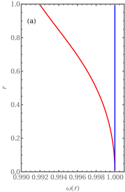
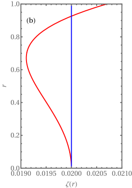
Figure 6: The instantaneous frequency (a) and instantaneous damping of system (33) together with the decoder (34). The blue line represents the naive calculation just from system (33) and the red lines represent the corrected values (29) and (30).

The geometry of the re-parametrisation is illustrated in figure 7.

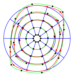
Figure 7: Geometry of the decoder (34). The blue grid represents the polar coordinate system with maximum radius $r=1$. The red curves are the images of the blue concentric circles under the decoder $\boldsymbol{W}$. The red dots are images of the intersection points of the blue circles with the blue radial lines under $\boldsymbol{W}$. The red dots do not fall onto the radial blue lines, which indicates a phase shift. The green curves correspond to the images of the blue concentric circles under the re-parametrised decoder $\tilde{\boldsymbol{W}}$ for the same parameters as the red curves. The amplitudes of the green curves are now the same as the amplitude of the corresponding blue curves. Due to the re-parametrisation, there is no phase shift between the black dots and the blue radial lines, on average.

4 ROM identification procedures

Here we describe our methodology of finding invariant foliations, manifolds and autoencoders. These steps involve methods described so far and further methods from the appendices. First we start with finding an invariant foliation together with the invariant manifold that has the same dynamics as the foliation.

• If the data is not from the full state space, especially when it is a scalar signal, we use a state-space reconstruction technique as described in appendix B. At this point we have data points $\boldsymbol{x}_{k},\boldsymbol{y}_{k}\in X$, $k=1,\ldots,N$.

• To ensure that the solution of (7) converges to the desired foliation, we calculate a linear approximation of the foliation. We only consider a small neighbourhood of the fixed point, where the dynamics is nearly linear. Hence, we define the index set $\mathcal{I}_{\rho}=\left\{k\in\left\{1,\ldots,N\right\}:\left|\boldsymbol{x}_{k}\right|<\rho\right\}$ with $\rho$ sufficiently small, but large enough that it encompasses enough data for linear parameter estimation.

  1. First we fit a linear model to the data using a create a least-squares method [9]. The linear map is assumed to be $\boldsymbol{y}_{k}=\boldsymbol{A}\boldsymbol{x}_{k}$, where the coefficient matrix is calculated as

     $$\boldsymbol{K} =\sum_{k\in\mathcal{I}_{\rho}}\left|\boldsymbol{x}_{k}\right|^{-2}\boldsymbol{x}_{k}\otimes\boldsymbol{x}_{k}^{T},$$

     $$\boldsymbol{L} =\sum_{k\in\mathcal{I}_{\rho}}\left|\boldsymbol{x}_{k}\right|^{-2}\boldsymbol{y}_{k}\otimes\boldsymbol{x}_{k}^{T},$$

     $$\boldsymbol{A} =\boldsymbol{L}\boldsymbol{K}^{-1}.$$

     Matrix $\boldsymbol{A}$ approximates the Jacobian $D\boldsymbol{F}\left(\boldsymbol{0}\right)$, which then can be used to identify the invariant subspaces $E^{\star}$ and $E$.

  2. The linearised version of foliation invariance (2) and manifold invariance (3) are

     $$\boldsymbol{S}_{1}\boldsymbol{U}_{1} =\boldsymbol{U}_{1}\boldsymbol{A}\;\text{and}$$

     $$\boldsymbol{W}_{1}\boldsymbol{S}_{1} =\boldsymbol{A}\boldsymbol{W}_{1},$$

     respectively. We also need to calculate the linearised version of our locally defined foliation (16), that is

     $$\boldsymbol{B}\boldsymbol{U}_{1}^{\perp}=\boldsymbol{U}_{1}^{\perp}\boldsymbol{A}.$$

     To find the unknown linear maps $\boldsymbol{U}_{1}$, $\boldsymbol{W}_{1}$, $\boldsymbol{U}_{1}^{\perp}$, $\boldsymbol{S}_{1}$ and $\boldsymbol{B}$ from $\boldsymbol{A}$, let us calculate the using real Schur decomposition of $\boldsymbol{A}$, that is $\boldsymbol{A}\boldsymbol{Q}=\boldsymbol{Q}\boldsymbol{H}$ or $\boldsymbol{Q}^{T}\boldsymbol{A}=\boldsymbol{H}\boldsymbol{Q}^{T}$, where $\boldsymbol{Q}$ is unitary and $\boldsymbol{H}$ is in an upper Hessenberg matrix, which is zero below the first subdiagonal. The Schur decomposition is calculated (or rearranged) such that the first $\nu$ column vectors, $\boldsymbol{q}_{1},\ldots,\boldsymbol{q}_{\nu}$ of $\boldsymbol{Q}$ span the required right invariant subspace $E$ and correspond to eigenvalues $\mu_{1},\ldots,\mu_{\nu}$. Therefore we find that $\boldsymbol{W}_{1}=\left[\boldsymbol{q}_{1},\ldots,\boldsymbol{q}_{\nu}\right]$. In addition, the last $n-\nu$ column vectors of $\boldsymbol{Q}$, when transposed, define a left-invariant subspace of $\boldsymbol{A}$. Therefore we define $\boldsymbol{U}_{1}^{\perp}=\left[\boldsymbol{q}_{\nu+1},\ldots,\boldsymbol{q}_{n}\right]^{T}$ and $\boldsymbol{B}_{1}=\boldsymbol{U}_{1}^{\perp}\boldsymbol{A}\boldsymbol{U}_{1}^{\perp T}$, which provides the initial guesses $\boldsymbol{U}^{\perp}\approx\boldsymbol{U}_{1}^{\perp}$ and $\boldsymbol{B}\approx\boldsymbol{B}_{1}$ in optimisation (20). In order to find the left-invariant subspace of $\boldsymbol{A}$ corresponding to the selected eigenvalues, we rearrange the Schur decomposition into $\hat{\boldsymbol{Q}}^{T}\boldsymbol{A}=\hat{\boldsymbol{H}}\hat{\boldsymbol{Q}}^{T}$, where $\hat{\boldsymbol{Q}}=\left[\hat{\boldsymbol{q}}_{1},\ldots,\hat{\boldsymbol{q}}_{n}\right]$ (using ordschur in Julia or Matlab) such that $\mu_{1},\ldots,\mu_{\nu}$ now appear last in the diagonal of $\hat{\boldsymbol{H}}$ at indices $\nu+1,\ldots,n$. This allows us to define $\boldsymbol{U}_{1}=\left[\hat{\boldsymbol{q}}_{n-\nu},\ldots,\hat{\boldsymbol{q}}_{n}\right]^{T}$ and $\boldsymbol{S}_{1}=\boldsymbol{U}_{1}\boldsymbol{A}\boldsymbol{U}_{1}^{T}$ which provides the initial guess for $D\boldsymbol{U}\left(\boldsymbol{0}\right)=\boldsymbol{U}_{1}$ and $D\boldsymbol{S}\left(\boldsymbol{0}\right)=\boldsymbol{S}_{1}$.

• We solve the optimisation problem (7) with the initial guess $D\boldsymbol{U}\left(\boldsymbol{0}\right)=\boldsymbol{U}_{1}$ and $D\boldsymbol{S}\left(\boldsymbol{0}\right)=\boldsymbol{S}_{1}$ as calculated in the previous step. We also prescribe the constraints that $D\boldsymbol{U}\left(\boldsymbol{0}\right)\left(D\boldsymbol{U}\left(\boldsymbol{0}\right)\right)^{T}=\boldsymbol{I}$ and that $\boldsymbol{U}\left(\boldsymbol{W}_{1}\boldsymbol{z}\right)$ is linear in $\boldsymbol{z}$. The numerical representation of the encoder $\boldsymbol{U}$ is described in appendix A.3.

• We perform a normal form transformation on map $\boldsymbol{S}$ and transform $\boldsymbol{U}$ into the new coordinates. The normal form $\boldsymbol{S}_{n}$ satisfies the invariance equation $\boldsymbol{U}_{n}\circ\boldsymbol{S}=\boldsymbol{S}_{n}\circ\boldsymbol{U}_{n}$ (c.f. equation (2)), where $\boldsymbol{U}_{n}:Z\to Z$ is a nonlinear map. We then replace $\boldsymbol{U}$ with $\boldsymbol{U}_{n}\circ\boldsymbol{U}$ and $\boldsymbol{S}$ with $\boldsymbol{S}_{n}$ as our ROM. This step is optional and only required if we want to calculate instantaneous frequencies and damping ratios. In a two-dimensional coordinate system, where we have a complex conjugate pair of eigenvalues $\mu_{1}=\overline{\mu}_{2}$, the real valued normal form is

  $$\begin{pmatrix}z_{1}\\ z_{2}\end{pmatrix}_{k+1}=\begin{pmatrix}z_{1}f_{r}\left(z_{1}^{2}+z_{2}^{2}\right)-z_{2}f_{r}\left(z_{1}^{2}+z_{2}^{2}\right)\\ z_{1}f_{i}\left(z_{1}^{2}+z_{2}^{2}\right)+z_{2}f_{r}\left(z_{1}^{2}+z_{2}^{2}\right)\end{pmatrix},$$ (35)

  which leads to the polar form (21) with $R\left(r\right)=r\sqrt{f_{r}^{2}\left(r^{2}\right)+f_{i}^{2}\left(r^{2}\right)}$ and $T\left(r\right)=\tan^{-1}\frac{f_{i}\left(r^{2}\right)}{f_{r}\left(r^{2}\right)}$. This normal form calculation is described in [55].

• To find the invariant manifold, we calculate a locally defined foliation (15) and solve the optimisation problem (20) to find the decoder $\boldsymbol{W}$ of invariant manifold $\mathcal{M}$. The initial guess in problem (20) is such that $\boldsymbol{U}^{\perp}=\boldsymbol{U}_{1}^{\perp}$ and $\boldsymbol{B}=\boldsymbol{B}_{1}$. We also need to set a $\kappa$ parameter, which is assumed to be $\kappa=0.2$ throughout the paper. We have found that results are not sensitive to the value of kappa except for extreme choices, such as $0,\infty$.

• In case of an oscillatory dynamics in a two-dimensional ROM, we recover the actual instantaneous frequencies and damping ratios using proposition (16).

The procedure for the Koopman eigenfunction calculation is the same as steps F1-F6, except that $\boldsymbol{S}$ is assumed to be linear. To identify an autoencoder, we use the same setup as in [17]. The numerical representation of the autoencoder is described in appendix A.2. We carry out the following steps

• We identify $\boldsymbol{W}_{1}$, $\boldsymbol{S}_{1}$ as in step F2 and set $\boldsymbol{U}=\boldsymbol{W}_{1}^{T}$ and $D\boldsymbol{S}\left(\boldsymbol{0}\right)=\boldsymbol{S}_{1}$

• Solve the optimisation problem

  $$\arg\min_{\boldsymbol{U},\boldsymbol{W}_{nl}}\sum_{k=1}^{N}\left\|\boldsymbol{y}_{k}\right\|^{-2}\left\|\boldsymbol{W}\left(\boldsymbol{U}\boldsymbol{y}_{k}\right)-\boldsymbol{y}_{k}\right\|^{2},$$

  which tries to ensure that $\boldsymbol{W}\circ\boldsymbol{U}$ is the identity, and finally solve

  $$\arg\min_{\boldsymbol{S}}\sum_{k=1}^{N}\left\|\boldsymbol{x}_{k}\right\|^{-2}\left\|\boldsymbol{W}\left(\boldsymbol{S}\left(\boldsymbol{U}\left(\boldsymbol{x}_{k}\right)\right)\right)-\boldsymbol{y}_{k}\right\|^{2}.$$

• Perform a normal form transformation on $\boldsymbol{S}$ by seeking the simplest $\boldsymbol{S}_{n}$ that satisfies $\boldsymbol{W}_{n}\circ\boldsymbol{S}_{n}=\boldsymbol{S}\circ\boldsymbol{W}_{n}$. This is similar to step F4, except that the normal form is in the style of the invariance equation of a manifold (3).

• Same as step F6, but applied to nonlinear map $\boldsymbol{S}_{n}$ and decoder $\boldsymbol{W}\circ\boldsymbol{W}_{n}$.

5 Examples

We are considering three examples. The first is a caricature model to illustrate all the techniques discussed in this paper and why certain techniques fail. The second example is a series of synthetic data sets with higher dimensionality, to illustrate the methods in more detail using a polynomial representations of the encoder with HT tensor coefficients (see appendix A.3). This example also illustrates two different methods to reconstruct the state space of the system from a scalar measurement. The final example is a physical experiment of a jointed beam, where only a scalar signal is recorded and we need to reconstruct the state space with our previously tested technique.

5.1 A caricature model

To illustrate the performance of autoencoders, invariant foliations and locally defined invariant foliations, we construct a simple two-dimensional map $\boldsymbol{F}$ with a node-type fixed point using the expression

$$\boldsymbol{F}\left(\boldsymbol{x}\right)=\boldsymbol{V}\left(\boldsymbol{A}\boldsymbol{V}^{-1}\left(\boldsymbol{x}\right)\right),$$ (36)

where

$$\boldsymbol{A}=\begin{pmatrix}\frac{9}{10}&0\\ 0&\frac{4}{5}\end{pmatrix},$$

the near-identity coordinate transformation is

$$\boldsymbol{V}\left(\boldsymbol{x}\right) =\begin{pmatrix}\begin{array}[]{l}x_{1}+\frac{1}{4}\left(x_{1}^{3}-3\left(x_{1}-1\right)x_{2}x_{1}+2x_{2}^{3}+\left(5x_{1}-2\right)x_{2}^{2}\right)\\ x_{2}+\frac{1}{4}\left(2x_{2}^{3}+\left(2x_{1}-1\right)x_{2}^{2}-x_{1}^{2}\left(x_{1}+2\right)\right)\end{array}\end{pmatrix},$$

and the state vector is defined as $\boldsymbol{x}=\left(x_{1},x_{2}\right)$. In a neighbourhood of the origin, transformation $\boldsymbol{V}$ has a unique inverse, which we calculate numerically. Map $\boldsymbol{F}$ is constructed such that we can immediately identify the smoothest (hence unique) invariant manifolds corresponding to the two eigenvalues of $D\boldsymbol{F}\left(0\right)$ as

$$\mathcal{M}_{\frac{9}{10}} =\left\{\boldsymbol{V}\left(z,0\right),z\in\mathbb{R}\right\},$$

$$\mathcal{M}_{\frac{4}{5}} =\left\{\boldsymbol{V}\left(0,z\right),z\in\mathbb{R}\right\}.$$

We can also calculate the leaves of the two invariant foliations as

$$\mathcal{L}_{\frac{9}{10},z} =\left\{\boldsymbol{V}\left(z,\overline{z}\right),\overline{z}\in\mathbb{R}\right\},$$ (37)

$$\mathcal{L}_{\frac{4}{5},z} =\left\{\boldsymbol{V}\left(\overline{z},z\right),\overline{z}\in\mathbb{R}\right\}.$$ (38)

To test the methods, we created 500 times 30 points long trajectories with initial conditions sampled from a uniform distribution over the rectangle $\left[-\frac{4}{5},\frac{4}{5}\right]\times\left[-\frac{1}{4},-\frac{1}{4}\right]$ to fit our ROM to.

We first attempt to fit an autoencoder to the data. We assume that the encoder, decoder and the nonlinear map $\boldsymbol{S}$ are

$$\boldsymbol{U}\left(x_{1},x_{2}\right) =x_{1},$$ (39)

$$\boldsymbol{W}\left(z\right) =\left(z,h\left(z\right)\right)^{T},$$ (40)

$$\boldsymbol{S}\left(z\right) =\lambda\left(z\right),$$ (41)

where $\lambda,h$ are polynomials of order-5. Our expressions already contain the invariant subspace $E=\mathrm{span}\left(1,0\right)^{T}$, which should make the fitting easier. Finally, we solve the optimisation problem (8). The result of the fitting can be seen in figure 8(a) as depicted by the red curve. The fitted curve is more dependent on the distribution of data than the actual position of the invariant manifold, which is represented by the blue dashed line in figure 8(a). Various other expressions for $\boldsymbol{U}$ and $\boldsymbol{W}$ were also tried that do not assume the direction of the invariant subspace $E$ with similar results.

To calculate the invariant foliation in the horizontal direction, we assume that

$$\left.\begin{array}[]{rl}\boldsymbol{U}\left(x_{1},x_{2}\right)&=x_{1}+u\left(x_{1},x_{2}\right)\\ \boldsymbol{S}\left(z\right)&=\lambda z\end{array}\right\},$$ (42)

where $u$ is an order-5 polynomial which lacks the constant and linear terms. The exact expression of $\boldsymbol{U}$ is not a polynomial, because it is the second coordinate of the inverse of function $\boldsymbol{V}$. The fitting is carried out by solving the optimisation problem (7). The result can be seen in figure 8(b), where the red curves are contour plots of the identified encoder $\boldsymbol{U}$ and the dashed blue lines are the leaves as defined by equation (37). Figure 8(c) is produced in the same way as 8(b), except that the encoder is defined as $\boldsymbol{U}\left(x_{1},x_{2}\right)=x_{2}+h\left(x_{1},x_{2}\right)$ and the blue lines are the leaves given by (38).

As we have discussed in section 2.2, a locally defined encoder can also be constructed from a decoder. In the expression of the encoder (15) we take

$$\boldsymbol{W}_{0}\left(z\right)=h\left(z\right)$$

and $\boldsymbol{U}^{\perp}=\left(0,1\right)$, where $h$ is an order-9 polynomial without constant and linear terms. The expressions for $\boldsymbol{U}$ and $\boldsymbol{S}$ were already found as (42), hence our approximate encoder becomes

$$\hat{\boldsymbol{U}}\left(\boldsymbol{x}\right)=x_{2}-h\left(x_{1}+u\left(x_{1},x_{2}\right)\right).$$

We solve the optimisation problem (20) with $\kappa=0.13$. We do not reconstruct the decoder $\boldsymbol{W}$, as it is straightforward to plot the level surfaces of $\hat{\boldsymbol{U}}$ directly. The result can be seen in figure 8(d), where the green line is the approximate invariant manifold (the zero level surface of $\hat{\boldsymbol{U}}$) and the red lines are other level surfaces of $\hat{\boldsymbol{U}}$.

In conclusion, this simple example shows that only invariant foliations can be fitted to data, autoencoders give spurious results.

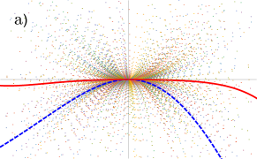
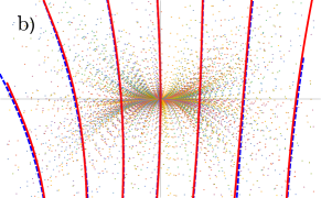
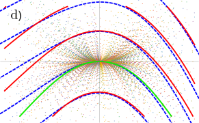
Figure 8: Identifying invariant objects in equation (36). The data contains 500 trajectories of length 30 with initial conditions picked from a uniform distribution; a) fitting an autoencoder (red continuous curve) does not reproduce the invariant manifold (blue dashed curve), instead it follows the distribution of data; (b) invariant foliation in the horizontal direction; c) invariant foliation in the vertical direction; d) an invariant manifold is calculated as the leaf of a locally defined invariant foliation. The green line is the invariant manifold. Each diagram represent the box $\left[-\frac{4}{5},\frac{4}{5}\right]\times\left[-\frac{1}{4},-\frac{1}{4}\right]$, the axes labels are intentionally hidden.

5.2 A ten-dimensional system

To create a numerically challenging example, we construct a ten-dimensional differential equation from five decoupled second-order nonlinear oscillators using two successive coordinate transformations. The system of decoupled oscillators is denoted by $\dot{\boldsymbol{x}}=\boldsymbol{f}_{0}\left(\boldsymbol{x}\right)$, where the state variable is in the form of

$$\boldsymbol{x}=\left(r_{1},\ldots,r_{5},\theta_{1},\ldots,\theta_{5}\right)$$

and the dynamics is given by

$$\begin{array}[]{ll}\dot{r}_{1}=-\frac{1}{500}r_{1}+\frac{1}{100}r_{1}^{3}-\frac{1}{10}r_{1}^{5},&\dot{\theta}_{1}=1+\frac{1}{4}r_{1}^{2}-\frac{3}{10}r_{1}^{4},\\ \dot{r}_{2}=-\frac{\mathrm{e}}{500}r_{2}-\frac{1}{10}r_{2}^{5},&\dot{\theta}_{2}=\mathrm{e}+\frac{3}{20}r_{2}^{2}-\frac{1}{5}r_{2}^{4},\\ \dot{r}_{3}=-\frac{1}{50}\sqrt{\frac{3}{10}}r_{3}+\frac{1}{100}r_{3}^{3}-\frac{1}{10}r_{3}^{5},&\dot{\theta}_{3}=\sqrt{30}+\frac{9}{50}r_{3}^{2}-\frac{19}{100}r_{3}^{4},\\ \dot{r}_{4}=-\frac{1}{500}\pi^{2}r_{4}+\frac{1}{100}r_{4}^{3}-\frac{1}{10}r_{4}^{5},&\dot{\theta}_{4}=\pi^{2}+\frac{4}{25}r_{4}^{2}-\frac{17}{100}r_{4}^{4},\\ \dot{r}_{5}=-\frac{13}{500}r_{5}+\frac{1}{100}r_{5}^{3},&\dot{\theta}_{5}=13+\frac{4}{25}r_{5}^{2}-\frac{9}{50}r_{5}^{4}.\end{array}$$ (43)

The first transformation brings the polar form of equation (43) into Cartesian coordinates using the transformation $\boldsymbol{y}=\boldsymbol{g}\left(\boldsymbol{x}\right)$, which is defined by $y_{2k-1}=r_{k}\cos\theta_{k}$ and $y_{2k}=r_{k}\sin\theta_{k}$. Finally, we couple all variables using the second nonlinear transformation $\boldsymbol{y}=\boldsymbol{h}\left(\boldsymbol{z}\right)$, which reads

$$\begin{array}[]{rlrl}y_{1}&=z_{1}+z_{3}-\frac{1}{12}z_{3}z_{5},&y_{2}&=z_{2}-z_{3},\\ y_{3}&=z_{3}+z_{5}-\frac{1}{12}z_{5}z_{7},&y_{4}&=z_{4}-z_{5},\\ y_{5}&=z_{5}+z_{7}+\frac{1}{12}z_{7}z_{9},&y_{6}&=z_{6}-z_{7},\\ y_{7}&=z_{7}+z_{9}-\frac{1}{12}z_{1}z_{9},&y_{8}&=z_{8}-z_{9},\\ y_{9}&=z_{9}+z_{1}-\frac{1}{12}z_{3}z_{1},&y_{10}&=z_{10}-z_{1},\end{array}$$ (44)

and where $\boldsymbol{y}=\left(y_{1},\ldots,y_{10}\right)$ and $\boldsymbol{z}=\left(z_{1},\ldots,z_{10}\right)$. The two transformations give us the differential equation $\dot{\boldsymbol{z}}=\boldsymbol{f}\left(\boldsymbol{z}\right)$, where

$$\boldsymbol{f}\left(\boldsymbol{z}\right)=\left[D\boldsymbol{g}^{-1}\left(\boldsymbol{h}\left(\boldsymbol{z}\right)\right)D\boldsymbol{h}\left(\boldsymbol{z}\right)\right]^{-1}\boldsymbol{f}_{0}\left(\boldsymbol{g}^{-1}\left(\boldsymbol{h}\left(\boldsymbol{z}\right)\right)\right).$$ (45)

The natural frequencies of our system at the origin are

$$\omega_{1}=1,\omega_{2}=\mathrm{e},\omega_{3}=\sqrt{30},\omega_{4}=\pi^{2},\omega_{5}=13$$

and the damping ratios are the same $\zeta_{1}=\cdots=\zeta_{5}=1/500$.

We select the first natural frequency to test various methods. We also test the methods on three types of data. Firstly, full state space information is used, secondly the state space is reconstructed from the signal $\xi_{k}=\frac{1}{10}\sum_{j=1}^{10}z_{k,j}$ using principal component analysis (PCA) as described in appendix B.1 with 16 PCA components, finally the state space is reconstructed from $\xi_{k}$ using a discrete Fourier transform (DFT) as described in appendix B.2. When data is recorded in state space form, $1000$ trajectories $16$ points long each with time step $\Delta T=0.1$ were created by numerically solving (45). Initial conditions were sampled from unit balls of radius $0.8$, $1.0$, $1.2$ and $1.4$ about the origin. The Euclidean norm of the initial conditions were uniformly distributed. The four data sets are labelled ST-1, ST-2, ST-3, ST-4 in the diagrams. For state space reconstruction, 100 trajectories, 3000 points each, with time step $\Delta T=0.01$ were created by numerically solving (45). The initial conditions for this data was similarly sampled from unit balls of radius $0.8$, $1.0$, $1.2$ and $1.4$ about the origin, such that the Euclidean norm of the initial conditions are uniformly distributed. The PCA reconstructed data are labelled PCA-1, PCA-2, PCA-3, PCA-4 and the DFT reconstructed data are labelled DFT-1, DFT-2, DFT-3, DFT-4.

The amplitude for each ROM is calculated as $A\left(r\right)=\sqrt{\frac{1}{2\pi}\int\left(\boldsymbol{w}^{\star}\cdot\boldsymbol{W}\left(r,\theta\right)\right)^{2}\mathrm{d}\theta}$, where $\boldsymbol{w}^{\star}=\frac{1}{10}\left(1,1,\ldots,1\right)$ for the state-space data and $\boldsymbol{w}^{\star}$ is calculated in appendices B.1, B.2 when state-space reconstruction is used. We can also attach an amplitude to each data point $\boldsymbol{x}_{k}$ through the encoder and the decoder. If the ROM assumes the normal form (35), the radial parameter $r$ is simply calculated as $r_{k}=\left\|\boldsymbol{U}\left(\boldsymbol{x}_{k}\right)\right\|$, hence the amplitude is $A\left(r_{k}\right)$.

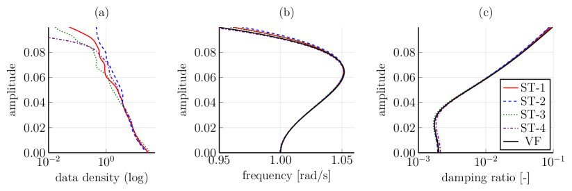
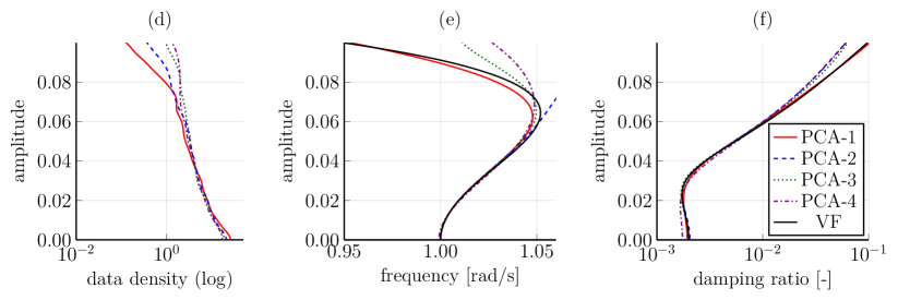
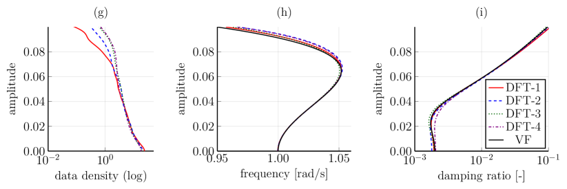
Figure 9: Instantaneous frequencies and damping ratios of differential equation (45) using invariant foliations. The first column shows the data density with respect to the amplitude $A\left(r\right)$, the second column is the instantaneous frequency and the third column is the instantaneous damping. The first row corresponds to state space data, the second row shows PCA reconstructed data and the third row is DFT reconstructed data. The data density is controlled by sampling initial conditions from different sized neighbourhoods of the origin.

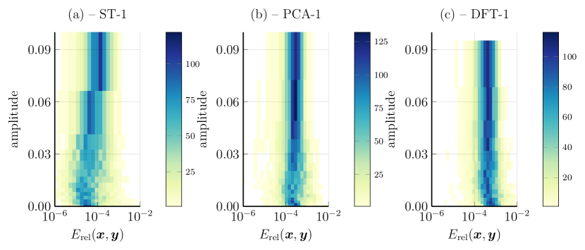
Figure 10: Histograms of the fitting error (46) for the data sets ST-1, PCA-1 and DFT-1 as a function of vibration amplitude. The distribution appears uniform with respect to the amplitude.

Figure 9 shows the result of our calculation for the three types of data. In the first column data density is displayed with respect to amplitude $A\left(r\right)$ in the ROM. Lower amplitudes have higher densities, because trajectories exponentially converge to the origin. In figure 9 we also display the identified instantaneous frequencies and damping ratios. The results are then compared to the analytically calculated frequencies and damping ratios labelled by VF.

State space data gives the closest match to the analytical reference (labelled as VF). We find that the PCA method cannot embed the data in a 10-dimesional space, only an 16-dimensional embedding is acceptable, but still inaccurate. Using a perfect reproducing filter bank (DFT) yields better results, probably because the original signal can be fully reconstructed and we expect a correct state-space reconstruction at small amplitudes. Indeed, the PCA results diverge at higher amplitudes, where the state space reconstruction is no longer valid. The author has also tried non-optimal delay embedding, with inferior results. None of the techniques had any problem with the less the challenging Shaw-Pierre example [52, 55] (data not shown).

Figure 10 shows the accuracy of the data fit as a function of the amplitude $A\left(r\right)$. The relative error displayed is defined by

$$E_{rel}\left(\boldsymbol{x},\boldsymbol{y}\right)=\frac{\left\|\boldsymbol{S}\left(\boldsymbol{U}\left(\boldsymbol{x}\right)\right)-\boldsymbol{U}\left(\boldsymbol{y}\right)\right\|}{\left\|\boldsymbol{U}\left(\boldsymbol{x}\right)\right\|}.$$ (46)

It turns out that the error is roughly independent of the amplitude, except for data set ST-1, which has lower errors at low amplitudes. The accuracy is the highest for state space data, while the accuracy of the DFT reconstructed data is slightly worse than for the PCA reconstructed data. In contrast, the comparison with the analytically calculated result is worse for the PCA data than for the DFT data. The reason is that PCA reconstruction cannot exactly reproduce the original signal from the identified components while the DFT method can.

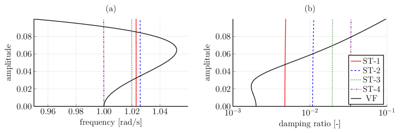
Figure 11: ROM by Koopman eigenfunctions. The same quantities are calculated as in figure 9, except that map $\boldsymbol{S}$ is assumed to be linear. There is some variation in the frequencies and damping ratios with respect to the amplitude due to the corrections in section 3, but accurate values could not be recovered as the linear approximation does not account for near internal resonances, as in formula (12).

When restricting map $\boldsymbol{S}$ to be linear, we are identifying Koopman eigenfunctions. Despite that linear dynamics is identified we should be able to reproduce the nonlinearities as illustrated in section 3. However, we also have near internal resonances as per equation (12), which make certain terms of encoder $\boldsymbol{U}$ large, which are difficult to find by optimisation. The result can be seen in figure 11. The identified frequencies and damping ratios show little variation with amplitude and mostly capture the average of the reference values. Fitting the Koopman eigenfunction achieves maximum and average values of $E_{rel}$ at $8.66\%$ and $0.189\%$ over data set ST-1, respectively. Better accuracy could be achieved using higher rank HT tensor coefficients in the encoder, which would significantly increase the number of model parameters. In contrast, fitting the invariant foliation to the same data set yields maximum and the average values of $E_{rel}$ at $2.21\%$ and $0.0118\%$, respectively (also illustrated in figure 10(a)). This better accuracy is achieved with a small number of extra parameters that make the two-dimensional map $\boldsymbol{S}$ nonlinear.

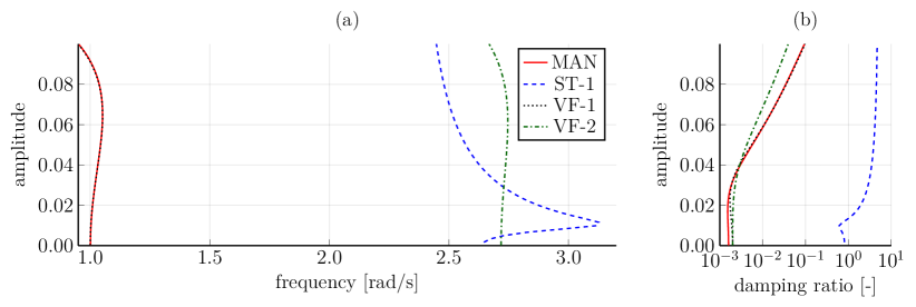
Figure 12: Data analysis by autoencoder. An autoencoder can recover system dynamics if all data is on the invariant manifold. For the solid line MAN, data was artificially forced to be on an a-priori calculated invariant manifold. However if the data is not on an invariant manifold, such as for data set ST-1, the autoencoder calculation is meaningless. The dotted line VF-1 represents the analytic calculation for the first natural frequency, the dash-dotted VF-2 depicts the analytic calculation for the second natural frequency of vector field (45).

Knowing that autoencoders are only useful if all the dynamics is on the manifold, we have synthetically created data consisting of trajectories with initial conditions from the invariant manifold of the first natural frequency. We used 800 trajectories, 24 points each with time-step $\Delta t=0.2$ starting on the manifold. Fitting an autoencoder to this data yields a good match in figure (12), the corresponding lines are labelled MAN. Then we tried dataset ST-1, that matched the reference best when calculating an invariant foliation. However, our data does not lie on a manifold and it is impossible to make $\boldsymbol{W}\circ\boldsymbol{U}$ close to the identity on our data. In fact the result (blue dashed line) is closer to the second mode of vibration (green dash-dotted curve), which seems to be the dominant vibration of the system.

5.3 Jointed beam

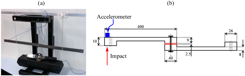
Figure 13: (a) Experimental setup. (b) Schematic of the jointed beam. The width of the beam (not shown) is 25mm. All measurements are in millimetres.

It is challenging to accurately model mechanical friction, hence data oriented methods can play a huge role in identifying dynamics affected by frictional forces. Therefore we analyse the data published in [59]. The experimental setup can be seen in figure 13. The two halves of the beam were joined together with an M6 bolt. The two interfaces of the beams were sandblasted to increase friction and a polished steel plate was placed between them, finally the bolt was tightened using four different torques: minimal torque so that the beam does not collapse under its own weight (denoted as 0 Nm), 1 Nm, 2.1 Nm and 3.1 Nm. The free vibration of the steel beam was recorded using an accelerometer placed at the end of the beam. The vibration was initiated using an impact hammer at the position of the accelerometer. Calibration data for the accelerometer is not available. For each torque value a number of 20 seconds long signals were recorded with sampling frequency of 2048 Hz. The impacts were of different magnitude so that the amplitude dependency of the dynamics could be tracked. In [59], a linear model was fitted to each signal and the first five vibration frequencies and damping ratios were identified. These are represented by various markers in figure 14. In order to make a connection between the peak impact force and the instantaneous amplitude we also calculated the peak root mean square (RMS) amplitude for signals with the largest impact force for each tightening torque and found that the average conversion factor between the peak RMS amplitude and the peak impact force was 443, which we used to divide the peak force and plot the equivalent peak RMS in figure 14. We also band filtered each trajectory with a 511 point FIR filter with 3 dB points at 30 Hz and 75 Hz and estimated the instantaneous frequency and damping ratios from two consecutive vibration cycles, which are then drawn as thick semi-transparent lines in figure 14 for each trajectory. It is worth noting that the more friction there is in the system, the less reproducible the frequencies and damping ratios become when using short trajectory segments for estimation.

To calculate the invariant foliation we used a 10-dimensional DFT reconstructed state space, to include all five captured frequencies, as described is appendix B.2. We chose $\kappa=0.2$ in the optimisation problem (20) when finding the invariant manifold. The result can be seen in figure 14. Since we do not have the ground truth for this system it is not possible to tell which method is more accurate, especially that our naive alternative calculation (thick semi-transparent lines) displays a wide spread of results.

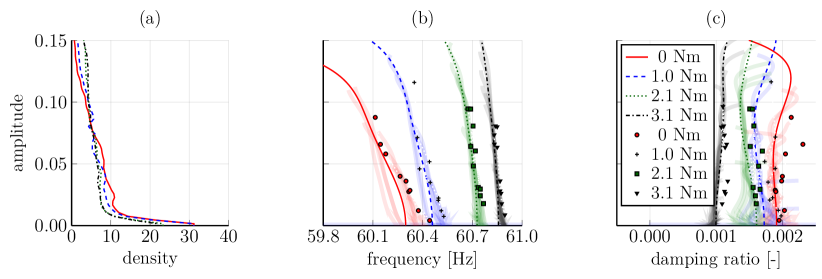
Figure 14: Instantaneous frequencies and damping ratios of the jointed beam set-up in figure 13. Solid red lines correspond to the invariant foliation of the system with minimal tightening torque, blue dashed lines with tightening torque of 2.1 Nm and green dotted lines with tightening torque of 3.1 Nm. The markers of the same colour show results calculated in [59] using curve fitting. (a) data density with respect to amplitude $A\left(r\right)$, (b) instantaneous frequency, (c) instantaneous damping ratio.

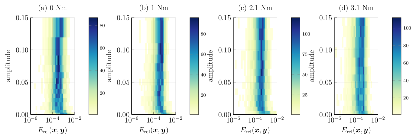
Figure 15: Histograms of the fitting error (46) for all four tightening torques of the jointed beam. Note that the errors look very similar despite that repeatability for lower tightening torques appear worse in figure 14.

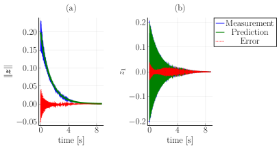
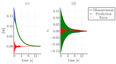
Figure 16: Reconstruction error of the foliation. (a,b) Reconstructing the first signal of the series of experimental data with 0 Nm tightening torque. (c,d) Reconstructing the first signal of the series of experimental data with 3.1 Nm tightening torque. The compared values are calculated through the encoder $\boldsymbol{z}=\boldsymbol{U}\left(\boldsymbol{x}_{k}\right)$ and the reconstructed values are from the iteration $\boldsymbol{z}_{k+1}=\boldsymbol{S}\left(\boldsymbol{z}_{k}\right)$. The amplitude error ($\left\|\boldsymbol{z}\right\|$) is minimal, however, over time phase error accumulates, hence direct comparison of a coordinate ($z_{1}$) can look unfavourable.

The fitting error to the invariant foliation can be assessed from the histograms in figure 15. The distribution of the error is very similar to the synthetic model, which is nearly uniform with respect to the vibration amplitude. It is also clear that there is no real difference in the fitting error for different tightening torques, which indicates that frictional dynamics can be accurately characterised using invariant foliations.

As a final test, we also assess whether the measured signal is reproduced by the invariant foliation $\left(\boldsymbol{U},\boldsymbol{S}\right)$ in figure 16. For this we apply the encoder $\boldsymbol{U}$ to our original signal $\boldsymbol{x}_{k}$, $k=1,\ldots,N$ and compare this signal to the one produced by the recursion $\boldsymbol{z}_{k+1}=\boldsymbol{S}\left(\boldsymbol{z}_{k}\right)$, where $\boldsymbol{z}_{1}=\boldsymbol{U}\left(\boldsymbol{x}_{1}\right)$. The instantaneous amplitude error in both cases of figures 16(a,c) was mostly due to high frequency oscillations that was not completely filtered out by the encoder $\boldsymbol{U}$ at the high amplitudes. The phase error seemed to have only accumulated for the lowest tightening torque (0 Nm) in figure 16(b). This is to be expected over long trajectories, since the fitting procedure only minimises the prediction error for a single time step. Unfortunately, accumulating phase error is rarely shown in the literature, where only short trajectories are compared, in contrast to the $28685$ and $25149$ time-steps that are displayed in figures 16(b,d), respectively.

6 Discussion

The main conclusion of this study is that only invariant foliations are suitable for ROM identification from off-line data. Using an invariant foliation avoids the need to use resonance decay [23], or waiting for the signal to settle near the most attracting invariant manifold [17], thereby throwing away valuable data. Using invariant foliations can make use of unstructured data with arbitrary initial conditions, such as impact hammer tests. Invariant foliations produce genuine ROMs and not only parametrise a-priori known invariant manifolds, like other methods [17, 18, 64]. We have shown that the high-dimensional function required to represent an encoder can be represented by polynomials with compressed tensor coefficients, which significantly reduces the computational and memory costs. Compressed tensors are also amenable to further analysis, such as singular value decomposition [26], which gives way to mathematical interpretations of the decoder $\boldsymbol{U}$. The low dimensional map $\boldsymbol{S}$ is also amenable to normal form transformations, which can be used to extract information such as instantaneous frequencies and damping ratios.

We have tested the related concept of Koopman eigenfuntions, which differs from an invariant foliation in that map $\boldsymbol{S}$ is assumed to be linear. If there are no internal resonances, Koopman eigenfunctions are theoretically equivalent to invariant foliations. However in numerical settings unresolved near internal resonances become important and therefore Koopman eigenfunctions become inadequate. We have also tried to fit autoencoders to our data [17], but apart from the artificial case where the invariant manifold was pre-computed, it performed even worse than Koopman eigenfunctions.

Fitting an invariant foliation to data is extremely robust when state space data is available. However, when the state space needed to be reproduced from a scalar signal, the results were not as accurate as we hoped for. While Taken’s theorem allows for any generic delay coordinates, in practice a non-optimal choice can lead to poor results. We were expecting that the embedding dimension at least for low amplitude signals would be the same as the attractor dimension. This is however not true if the data also includes higher amplitude points. Despite not being theoretically optimal, we have found that perfect reproducing filter banks produce accurate results for low amplitude signals and at the same time provide a state-space reconstruction with the same dimensionality as that of the attractor. Future work should include exploring various state-space reconstruction techniques in combination with fitting an invariant foliation to data.

We did not fully explore the idea of locally defined invariant foliations in remark 15, which can lead to computationally efficient methods. Further research can also be directed towards cases, where the data is on a high-dimensional submanifold of an even higher dimensional vector space $X$. This is where an autoencoder and invariant foliation may be combined.

Appendix A Implementation details

In this appendix we deal with how to represent invariant foliations, locally defined invariant foliations and autoencoders. We also describe our specific techniques to carry out optimisation on these representations.

A.1 Dense polynomial representation

The nonlinear map $\boldsymbol{S}$, the polynomial part of the locally defined invariant foliation $\boldsymbol{W}_{0}$ and the decoder part an autoencoder are represented by dense polynomials, that we define here.

A polynomial $\boldsymbol{P}:Z\to X$ of order $d$ is represented as a linear combination of monomials formed from the coordinates of vectors of $Z$. First we define what we mean by a monomial and how we order them. Given a basis in $Z$ with $\nu=\dim Z$, we can represent each vector $\boldsymbol{z}\in Z$ by $\boldsymbol{z}=\left(z_{1},z_{2},\ldots,z_{\nu}\right)$. Then we define non-negative integer vectors $\boldsymbol{m}=\left(m_{1},\ldots,m_{\nu}\right)\in\mathbb{N}^{\nu}$ and finally define a monomial of $\boldsymbol{z}$ by $\boldsymbol{z}^{\boldsymbol{m}}=z_{1}^{m_{1}}z_{2}^{m_{2}}\cdots z_{\nu}^{m_{\nu}}$. We also need an ordered set of integer exponents, which is denoted by

$$\mathfrak{M}_{c,d}=\left\{\boldsymbol{m}\in\mathbb{N}^{\nu}:c\leq m_{1}+\cdots+m_{\nu}\leq d\right\}.$$

The ordering of $\mathfrak{M}_{c,d}$ is such that $\boldsymbol{m}<\boldsymbol{n}$ if there exists $k\leq\nu$ and $m_{j}<n_{j}$ for all $j=1,\ldots,k$. The cardinality of set $\mathfrak{M}_{c,d}$ is denoted by $\#\left(\nu,c,d\right)$. Therefore we can also write that $\mathfrak{M}_{c,d}=\left\{\boldsymbol{m}_{1},\boldsymbol{m}_{2},\ldots,\boldsymbol{m}_{\#\left(\nu,c,d\right)}\right\}$. Using the ordered notation of monomials, a polynomial $\boldsymbol{P}$ containing terms at least order $c$ up to order-$d$ is represented by a matrix $\underline{\boldsymbol{P}}\in\mathbb{R}^{n\times\#\left(\nu,c,d\right)}$, such that

$$\boldsymbol{P}\left(\boldsymbol{z}\right)=\underline{\boldsymbol{P}}\left(\boldsymbol{z}^{\boldsymbol{m}_{1}},\boldsymbol{z}^{\boldsymbol{m}_{2}},\cdots,\boldsymbol{z}^{\boldsymbol{m}_{\#\left(\nu,c,d\right)}}\right)^{T}.$$

We also call such polynomials order-$\left(c,d\right)$ polynomials. For optimisation purposes order-$\left(c,d\right)$ polynomials form an Euclidean manifold and therefore no constraint is placed on matrix $\underline{\boldsymbol{P}}$.

A.2 Autoencoder representation

A polynomial autoencoder of order $d$ (as defined in [17]) is represented by an orthogonal matrix $\underline{\boldsymbol{U}}\in\mathbb{R}^{n\times\nu}$ ($\underline{\boldsymbol{U}}^{T}\underline{\boldsymbol{U}}=\boldsymbol{I}$) and an order-$\left(2,d\right)$ polynomial $\boldsymbol{W}$, represented by matrix $\underline{\boldsymbol{W}}\in\mathbb{R}^{n\times\#\left(\nu,2,d\right)}$. The associated encoder is given by $\boldsymbol{U}\left(\boldsymbol{x}\right)=\underline{\boldsymbol{U}}^{T}\boldsymbol{x}$ and the decoder is given by $\boldsymbol{W}\left(\boldsymbol{z}\right)=\boldsymbol{U}\boldsymbol{z}+\boldsymbol{W}\left(\boldsymbol{z}\right)$, which must satisfy the additional constraint $\boldsymbol{U}\left(\boldsymbol{W}\left(\boldsymbol{z}\right)\right)=\boldsymbol{z}$, that in terms of our matrices means $\underline{\boldsymbol{U}}^{T}\underline{\boldsymbol{W}}=\boldsymbol{0}$. In summary, we have the constraints

$$\begin{array}[]{rl}\underline{\boldsymbol{U}}^{T}\underline{\boldsymbol{U}}&=\boldsymbol{I},\\ \underline{\boldsymbol{U}}^{T}\underline{\boldsymbol{W}}&=\boldsymbol{0},\end{array}$$ (47)

which turns the admissible set of matrices $\underline{\boldsymbol{U}},\,\underline{\boldsymbol{W}}$ into a matrix manifold. We call this manifold the orthogonal autoencoder manifold and denote it by $\mathit{OAE}_{n,\nu,\#\left(\nu,2,d\right)}$. In paper [17], the authors also consider the case when the decoder is decoupled from the encoder. In this case $\boldsymbol{W}\left(\boldsymbol{z}\right)$ does not include the orthogonal matrix $\boldsymbol{U}$ and therefore $\boldsymbol{W}\left(\boldsymbol{z}\right)$ is represented by matrix $\underline{\boldsymbol{W}}\in\mathbb{R}^{n\times\#\left(\nu,1,d\right)}$, which also includes linear terms. The constraint on matrices $\underline{\boldsymbol{U}},\,\underline{\boldsymbol{W}}$ is therefore different

$$\begin{array}[]{rl}\underline{\boldsymbol{U}}^{T}\underline{\boldsymbol{U}}&=\boldsymbol{I},\\ \underline{\boldsymbol{U}}^{T}\underline{\boldsymbol{W}}&=\boldsymbol{M},\end{array}$$ (48)

where matrix $\boldsymbol{M}$ represents the identity polynomial with respect to the monomials $\mathfrak{M}_{1,d}$. We call the resulting matrix manifold the generalised orthogonal autoencoder manifold and denote it by $\mathit{GOAE}_{\boldsymbol{M},n,\nu,\#\left(\nu,1,d\right)}$. Unfortunately, this generalised autoencoder leads to an ill-defined optimisation problem. Indeed, if all the data is on an invariant manifold (the only sensible case), then the directions encoded by $\boldsymbol{U}$ are not defined by the data, because any transversal direction is equally suitable for projecting the data. In our numerical test $\boldsymbol{U}$ quickly degenerated and led to spurious results. Nevertheless, due to the similar formulation we treat both cases at the same time, because $\mathit{OAE}_{n,m,l}$ is a particular case of $\mathit{GOAE}_{\boldsymbol{M},n,m,l}$ with $\boldsymbol{M}$ being equal to zero. The details of how projections and retractions are calculated for $\mathit{GOAE}_{\boldsymbol{M},n,m,l}$ are presented in section A.5.1.

A.3 Compressed polynomial representation with hierarchical tensor coefficients

To represent encoders of invariant foliations we need to approximate high-dimensional functions. Dense polynomials are not suitable to represent high-dimensional functions, because the number of required parameters increase combinatorially. One approach is to use multi-layer neural networks [31, 24], however their training can be problematic [42]. Standard training methods take a long time and they rarely reach the global minimum (and there is no free lunch [63]). In addition, the approximation can overfit the data, that is the accuracy on unseen data can be significantly worse than on the training data. In terms of the geometry of neural networks, they do not form a differentiable manifold and therefore parameters may tend to infinity without minimising the loss function [47].

To represent encoders we still use polynomials, except that the polynomial coefficients are represented by compressed tensors in the hierarchical Tucker (HT) format. This tensor format was introduced in [28] and demonstrated to solve many problems [27] that would normally wrestle with the ’curse of dimensionality’ [4]. In chemisty and physics a somewhat different but related format, the matrix product state [46] is frequently used and in other problems a particular type of HT representation the tensor train format [44] is used. However, the most important property of HT tensors is that they form a smooth quotient manifold and therefore suitable to use in optimisation problems [60].

To define the format, we partly follow the notation of [60] in our definitions. First, we need to define the dimension tree.

Definition 21.

Given an order $d$, a dimension tree $T$ is a non-trivial rooted binary tree whose nodes can be labelled by subsets of $\left\{1,2,\ldots,d\right\}$ such that

1. the root has the label $t_{r}=\left\{1,2,\ldots,d\right\}$, and

2. every node $t\in T$, which is not a leaf has two descendants, $t_{1}$ and $t_{2}$ that form an ordered partition of $t$, that is,

   $$t_{1}\cup t_{2}=t\quad\text{and}\quad\mu<\nu\;\text{for all}\;\mu\in t_{1},\nu\in t_{2}.$$

The set of leaf nodes is denoted by $L=\left\{\left\{1\right\},\left\{2\right\},\ldots,\left\{d\right\}\right\}$.

Definition 22.

Let $T$ be a dimension tree and $\boldsymbol{k}=\left(k_{t}\right)_{t\in T}$ a set of positive integers. The hierarchical Tucker format for $\mathbb{R}^{n_{0}\times n_{1}\times\cdots\times n_{d}}$ is defined as follows

1. For a leaf node $U_{t}$ is an orthonormal matrix, such that $U_{t}\in\mathbb{R}^{k_{t}\times n_{t}}$ with elements $U_{t}\left(i;j\right)$, where $i=1\ldots k_{t}$, $j=1\ldots n_{t}$

2. For not a leaf node with $t=t_{1}\cup t_{2}$ we define

   $$U_{t}\left(p;i_{1},\ldots,i_{\left|t_{1}\right|},j_{1},\ldots,j_{\left|t_{2}\right|}\right)=\sum_{q=1}^{k_{t_{1}}}\sum_{r=1}^{k_{t_{2}}}B_{t}\left(p,q,r\right)U_{t_{1}}\left(q;i_{1},\ldots,i_{\left|t_{1}\right|}\right)U_{t_{2}}\left(r;j_{1},\ldots,j_{\left|t_{2}\right|}\right),$$ (49)

   where $\left|t\right|$ stands for the number of indices in label $t$.

The definition is recursive, hence data storage for $U_{t}$ is only required for the leaf nodes, and for non-leaf nodes only storing $B_{t}$ is sufficient. In other words, the set of matrices

$$\left\{U_{t}:t\in L\right\}\cup\left\{B_{t}:t\in T\setminus L\right\}$$

fully specifies a HT tensor. For each node, apart from the root node $t_{r}$, one can apply a transformation, which does not change the resulting tensor. That is, for $t\neq t_{r}$ define $\tilde{U}_{t}=A_{t}U_{t}$ and $\tilde{B}_{t}=B_{t}\times_{2,3}A_{t_{1}}^{-1}\otimes A_{t_{2}}^{-1}$, where $A_{t}\in\mathbb{R}^{k_{t}\times k_{t}}$ are invertible matrices. Without restricting generality, we can stipulate that the leaf nodes $U_{t}$ and matricisation of $B_{t}$ with respect to the first index are also orthogonal matrices, which means that transformations $A_{t}$ must be unitary to preserve orthogonality. This identity transformation defines an equivalence relation between parametrisations of a HT tensor and therefore the HT format is a quotient manifold as described in [8, chapter 7]. Using a quotient manifold would prevent us from optimising for the matrices $U_{t}$, $B_{t}$ individually, as we need to treat the whole HT tensor as a single entity. In addition, we could not find any example in the literature, where a HT tensor was treated as a quotient manifold. Instead, we simply assume a simpler structure, that is, $B_{t_{r}}$ is on a Euclidean manifold and the rest of the coefficients $B_{t}$ and $U_{t}$ are orthogonal matrices and therefore elements of Stiefel manifolds, which is the running example in [8]. This way we have the HT format as an element of a product manifold, where each coefficient matrix remains independent of each other. It is also possible to calculate singular values of HT tensors. Vanishing singular values indicate that the required quantity is well-approximated and that the HT tensor can be simplified to include less terms. This further adds to our ability to identify parsimonious models. In what follows, we use balanced dimension trees and up to rank six matrices $U_{t}$, $B_{t}$ for simplicity.

Using notation (49), we can write the encoders as

$$\boldsymbol{U}\left(\boldsymbol{x}\right)=\boldsymbol{U}^{1}\boldsymbol{x}+\sum_{d=2}^{p}\sum_{i_{1}\cdots i_{d}=1}^{n}U_{t_{r}}^{d}\left(\cdot;i_{1},\ldots,i_{d}\right)x_{i_{1}}\cdots x_{i_{d}},$$ (50)

where $\boldsymbol{U}^{1}$ is an orthogonal matrix, similarly element of a Stiefel manifold. We also apply the constraint that $\boldsymbol{U}\left(\boldsymbol{W}_{1}\boldsymbol{z}\right)$ must be linear. This simply means that for the nonlinear terms of $\boldsymbol{U}$ the data must not include components in the $\boldsymbol{W}_{1}$ direction. This can be achieved by projecting our data, that is $\hat{\boldsymbol{x}}=\boldsymbol{U}_{1}^{\perp}\boldsymbol{x}$, where $\boldsymbol{U}_{1}^{\perp}$ is obtained in step F2 of the invariant foliation identification process of section 4 and consists of row vectors that are orthogonal to the column vectors of $\boldsymbol{W}_{1}$. Therefore our constrained encoder assumes the form of

$$\boldsymbol{U}\left(\boldsymbol{x}\right)=\boldsymbol{U}^{1}\boldsymbol{x}+\sum_{d=2}^{p}\sum_{i_{1}\cdots i_{d}=1}^{n}U_{t_{r}}^{d}\left(\cdot;i_{1},\ldots,i_{d}\right)\hat{x}_{i_{1}}\cdots\hat{x}_{i_{d}}.$$

A.4 Optimisation techniques

Given our compressed representation of the encoder in the form (50), we can now discuss how to solve the optimisation problem (7).

HT tensors, which make up the parametrisation of the encoder $\boldsymbol{U}$, depend linearly on each matrix $B_{t}^{d}$, $U_{t}^{d}$ individually. Therefore, it is beneficial to carry out the optimisation for each matrix component individually, and cycle through all matrix components a number of times until convergence is reached. This is called batch coordinate descent [43]. The complicating factor in this approach is that the encoder also appears as an inner function of map $\boldsymbol{S}$ and therefore the dependence of the objective function becomes nonlinear on matrices $B_{t}$, $U_{t}$. For optimisation in each coordinate we use the second order trust-region method [20] as we can explicitly calculate the Hessian of the objective function with respect to each matrix $B_{t}^{d},U_{t}^{d}$ and the parameters of $\boldsymbol{S}$. We only take a limited number of steps with the trust region method, as we cycle through all parameter matrices. The algorithm cycles through each tensor and the parameters of $\boldsymbol{S}$ in a given order, but for each tensor of order $d$, only the coefficient matrix for which the gradient of the objective function is the largest is optimised for. This is a variant of the Gauss-Southwell algorithm [41]. We found that this technique, as it eliminates unnecessary optimisation steps for parameters that do not influence the objective function much, converges relatively fast. Attempts to use off-the-shelf optimisers were fruitless, due to computational costs.

To identify locally defined foliations we use the Riemannian trust region method and for identifying autoencoders, we use the Riemannian BFGS quasi-Newton technique from software package [5].

A.5 Projections and retractions on matrix manifolds

As we perform optimisation on matrix manifolds, we also require an orthogonal projection from the ambient space to the tangent space to the manifold and a retraction [8, 1]. The advantage of optimising on a manifold instead of using standard constrained optimisation is that retractions and projections are generally easier to evaluate than solving the constraints using generic methods.

Let us assume that our matrix manifold $\mathcal{M}$ is embedded into the Euclidean space $\mathcal{E}$. As computers deal with lists of numbers, we only have a cost function defined on $\mathcal{E}$, which we denote by $\overline{F}:\mathcal{E}\to\mathbb{R}$, instead on the manifold $F:\mathcal{M}\to\mathbb{R}$. Carrying out optimisation on $\mathcal{M}$ therefore requires various corrections when we use cost function $\overline{F}$. The gradient $\nabla F$ on $\mathcal{M}$ is a map from $\mathcal{M}$ to the tangent bundle $T\mathcal{M}$. Generally $\overline{F}$ does not map into $T\mathcal{M}$, therefore a projection is necessary. In particular, for a specific point $\boldsymbol{p}\in\mathcal{M}$, the projection is the linear map $\boldsymbol{P}_{\boldsymbol{p}}:T_{\boldsymbol{p}}\mathcal{E}\to T_{\boldsymbol{p}}\mathcal{M}$ and the gradient is calculated as

$$\nabla F\left(\boldsymbol{p}\right)=\boldsymbol{P}_{\boldsymbol{p}}\nabla\overline{F}\left(\boldsymbol{p}\right).$$

A simple gradient descent method would move in the direction of the gradient, however that is not necessarily on manifold $\mathcal{M}$, so we need to bring the result back to $\mathcal{M}$ using a retraction. A retraction is a map $R_{\boldsymbol{p}}\left(\boldsymbol{X}\right):T\mathcal{M}\to\mathcal{M}$ for which $DR_{\boldsymbol{p}}\left(\boldsymbol{0}\right)\boldsymbol{Y}=\boldsymbol{Y}$. A retraction is supposed to approximate the so-called exponential map on the tangent space, which produces the geodesics along the manifold in the direction of the tangent vector $\boldsymbol{X}$ up to the length of $\boldsymbol{X}$. A second order approximation of the exponential retraction is the solution of the minimisation problem

$$R_{\boldsymbol{p}}\left(\boldsymbol{X}\right)=\arg\min_{\boldsymbol{q}\in\mathcal{M}}\left\|\boldsymbol{p}+\boldsymbol{X}-\boldsymbol{q}\right\|^{2}.$$ (51)

Projection like retractions are explained in detail in [2]. Using a retraction we can pull back our result onto the manifold. The Hessian of $F$ can be defined in terms of a second order retraction $R$. If we assume that $\tilde{F}\left(\boldsymbol{p},\boldsymbol{X}\right)=\overline{F}\left(R_{\boldsymbol{p}}\left(\boldsymbol{P}_{\boldsymbol{p}}\boldsymbol{X}\right)\right)$, then the Hessian is

$$D^{2}F\left(\boldsymbol{p}\right)=D_{2}^{2}\tilde{F}\left(\boldsymbol{p},\boldsymbol{0}\right).$$

The expression of the Hessian can be simplified in many ways, which is described, e.g., in [8].

In what follows we detail two matrix manifolds that do not appear in the literature and are specific to our problems. We also use the Stiefel manifold of orthogonal matrices that is covered in many publications [8]. In particular, we use the so-called polar retraction of the Stiefel manifold, which is equivalent to equation (51). For our specific matrix manifolds we solve (51).

A.5.1 Autoencoder manifold

The two matrices $\boldsymbol{p}_{1}=\underline{\boldsymbol{U}}\in\mathbb{R}^{n\times m}$ , $\boldsymbol{p}_{2}=\underline{\boldsymbol{W}}\in\mathbb{R}^{n\times l}$ that satisfy the constraints (47) represent an orthogonal autoencoder form the matrix manifold $\mathcal{M}=\mathit{GOAE}_{\boldsymbol{M},n,m,l}$, which is defined by the zero-level set of submersion

$$\boldsymbol{h}\left(\boldsymbol{p}_{1},\boldsymbol{p}_{2}\right)=\begin{pmatrix}\boldsymbol{p}_{1}^{T}\boldsymbol{p}_{1}-\boldsymbol{I}\\ \boldsymbol{p}_{1}^{T}\boldsymbol{p}_{2}-\boldsymbol{M}\end{pmatrix}.$$

For $\mathcal{M}$ to be a manifold the derivative $D\boldsymbol{h}$ must have full rank. Indeed, we calculate that

$$D\boldsymbol{h}\left(\boldsymbol{p}_{1},\boldsymbol{p}_{2}\right)\left(\boldsymbol{X}_{1},\boldsymbol{X}_{2}\right)=\begin{pmatrix}\boldsymbol{X}_{1}^{T}\boldsymbol{p}_{1}+\boldsymbol{p}_{1}^{T}\boldsymbol{X}_{1}\\ \boldsymbol{X}_{1}^{T}\boldsymbol{p}_{2}+\boldsymbol{p}_{1}^{T}\boldsymbol{X}_{2}\end{pmatrix},$$

and substitute $\boldsymbol{X}_{1}=\boldsymbol{p}_{1}\boldsymbol{A}$, $\boldsymbol{X}_{2}=\boldsymbol{p}_{1}\boldsymbol{B}$, which yields

$$D\boldsymbol{h}\left(\boldsymbol{p}_{1},\boldsymbol{p}_{2}\right)\left(\boldsymbol{X}_{1},\boldsymbol{X}_{2}\right)=\begin{pmatrix}\boldsymbol{A}^{T}+\boldsymbol{A}\\ \boldsymbol{B}\end{pmatrix}.$$

Since $\boldsymbol{A}$ and $\boldsymbol{B}$ are arbitrary matrices the range of $D\boldsymbol{h}$ is the full set of symmetric and general matrices, that is, $D\boldsymbol{h}$ has full rank, hence $\mathcal{M}$ is an embedded manifold.

Tangent space.

The tangent space $T_{\left(\boldsymbol{p}_{1},\boldsymbol{p}_{2}\right)}\mathcal{M}$ is defined as the null space of $D\boldsymbol{h}\left(\boldsymbol{p}\right)$, that is

$$T_{\left(\boldsymbol{p}_{1},\boldsymbol{p}_{2}\right)}\mathcal{M}=\left\{\boldsymbol{X}\in\mathbb{R}^{n\times m}:D\boldsymbol{h}\left(\boldsymbol{p}_{1},\boldsymbol{p}_{2}\right)\left(\boldsymbol{X}_{1},\boldsymbol{X}_{2}\right)=\left(\boldsymbol{0},\boldsymbol{0}\right)\right\}.$$

We define $\boldsymbol{p}^{\perp}\in\mathbb{R}^{n\times\left(n-m\right)}$ by $\boldsymbol{p}^{\perp T}\boldsymbol{p}^{\perp}=\boldsymbol{I}$ and $\boldsymbol{p}^{T}\boldsymbol{p}^{\perp}=\boldsymbol{0}$, hence the direct sum of ranges of $\boldsymbol{p}$ and $\boldsymbol{p}^{\perp}$ span $\mathbb{R}^{n}$. To characterise the tangent space we decompose $\boldsymbol{X}_{1}=\boldsymbol{p}_{1}\boldsymbol{A}_{1}+\boldsymbol{p}_{1}^{\perp}\boldsymbol{B}_{1}$, $\boldsymbol{X}_{2}=\boldsymbol{p}_{1}\boldsymbol{A}_{2}+\boldsymbol{p}_{1}^{\perp}\boldsymbol{B}_{2}$, and find that

$$D\boldsymbol{h}\left(\boldsymbol{p}_{1},\boldsymbol{p}_{2}\right)\left(\boldsymbol{X}_{1},\boldsymbol{X}_{2}\right)=\begin{pmatrix}\boldsymbol{A}_{1}^{T}+\boldsymbol{A}_{1}\\ \boldsymbol{B}_{1}^{T}\boldsymbol{p}_{1}^{\perp T}\boldsymbol{p}_{2}+\boldsymbol{A}_{2}\end{pmatrix}.$$ (52)

For (53) to equal zero, $\boldsymbol{A}_{1}$ must be antisymmetric, $\boldsymbol{B}_{1}$, $\boldsymbol{B}_{2}$ can be arbitrary and $\boldsymbol{A}_{2}=-\boldsymbol{B}_{1}^{T}\boldsymbol{p}_{1}^{\perp T}\boldsymbol{p}_{2}$.

Normal space.

We use $\boldsymbol{X}_{1}=\boldsymbol{p}_{1}\boldsymbol{A}_{1}+\boldsymbol{p}_{1}^{\perp}\boldsymbol{B}_{1}$, $\boldsymbol{X}_{2}=-\boldsymbol{p}_{1}\boldsymbol{B}_{1}^{T}\boldsymbol{p}_{1}^{\perp T}\boldsymbol{p}_{2}+\boldsymbol{p}_{1}^{\perp}\boldsymbol{B}_{2}$ to represent an element of the tangent space and $\boldsymbol{Y}_{1}=\boldsymbol{p}_{1}\boldsymbol{K}_{1}+\boldsymbol{p}_{1}^{\perp}\boldsymbol{L}_{1}$, $\boldsymbol{Y}_{2}=\boldsymbol{p}_{1}\boldsymbol{K}_{2}+\boldsymbol{p}_{1}^{\perp}\boldsymbol{L}_{2}$ to represent an arbitrary element of the ambient space. For $\left(\boldsymbol{Y}_{1},\boldsymbol{Y}_{2}\right)$ to be a normal vector in $N_{\left(\boldsymbol{p}_{1},\boldsymbol{p}_{2}\right)}\mathcal{M}$ equation

$$\left\langle\boldsymbol{X}_{1},\boldsymbol{Y}_{1}\right\rangle+\left\langle\boldsymbol{X}_{2},\boldsymbol{Y}_{2}\right\rangle =0$$ (53)

must hold for all $\boldsymbol{B}_{1}$, $\boldsymbol{B}_{2}$ and $\boldsymbol{A}_{1}$ antisymmetric matrices. Therefore we expand (53) into

$$\left\langle\boldsymbol{A}_{1},\boldsymbol{K}_{1}\right\rangle+\left\langle\boldsymbol{B}_{1},\boldsymbol{L}_{1}\right\rangle-\left\langle\boldsymbol{B}_{1}^{T}\boldsymbol{p}_{1}^{\perp T}\boldsymbol{p}_{2},\boldsymbol{K}_{2}\right\rangle+\left\langle\boldsymbol{B}_{2},\boldsymbol{L}_{2}\right\rangle=0.$$ (54)

To explore what parameters are allowed, we consider (54) term-by-term. If we set $\boldsymbol{B}_{1}=\boldsymbol{0}$, $\boldsymbol{B}_{2}=\boldsymbol{0}$, then what remains is $\left\langle\boldsymbol{A}_{1},\boldsymbol{K}_{1}\right\rangle=0$ for all $\boldsymbol{A}_{1}$ anti-symmetric. This constraint holds if and only if $\boldsymbol{K}_{1}$ is symmetric. Now we set $\boldsymbol{A}_{1}=\boldsymbol{0},\boldsymbol{B}_{1}=\boldsymbol{0}$, which leads to $\left\langle\boldsymbol{B}_{2},\boldsymbol{L}_{2}\right\rangle=0$ for all $\boldsymbol{B}_{2}$, hence we must have $\boldsymbol{L}_{2}=\boldsymbol{0}$. Finally we set $\boldsymbol{A}_{1}=\boldsymbol{0},\boldsymbol{B}_{2}=\boldsymbol{0}$, which gives us

$$\left\langle\boldsymbol{B}_{1},\boldsymbol{L}_{1}\right\rangle-\left\langle\boldsymbol{B}_{1}^{T}\boldsymbol{p}_{1}^{\perp T}\boldsymbol{p}_{2},\boldsymbol{K}_{2}\right\rangle =0,$$

$$\left\langle\boldsymbol{B}_{1},\boldsymbol{L}_{1}\right\rangle-\left\langle\boldsymbol{p}_{2},\boldsymbol{p}_{1}^{\perp}\boldsymbol{B}_{1}\boldsymbol{K}_{2}\right\rangle =0$$

or in index notation

$$B_{1ij}L_{1ij}-p_{2ji}p_{1jk}^{\perp}B_{1kl}K_{2li}=0.$$ (55)

Now we differentiate (55) with respect to $\boldsymbol{B}_{1}$, which gives

$$L_{1rs}-p_{2ji}p_{1jr}^{\perp}K_{2si}=0\;\implies\;\boldsymbol{L}_{1}=\boldsymbol{p}_{1}^{\perp T}\boldsymbol{p}_{2}\boldsymbol{K}_{2}^{T}.$$

In conclusion the normal space is given by matrices of the form

$$\begin{array}[]{rl}\boldsymbol{Y}_{1}&=\boldsymbol{p}_{1}\boldsymbol{K}_{1}+\boldsymbol{p}_{1}^{\perp}\boldsymbol{p}_{1}^{\perp T}\boldsymbol{p}_{2}\boldsymbol{K}_{2}^{T},\\ \boldsymbol{Y}_{2}&=\boldsymbol{p}_{1}\boldsymbol{K}_{2},\end{array}$$ (56)

where $\boldsymbol{K}_{1}$ symmetric and $\boldsymbol{K}_{2}$ is a general matrix.

Projection to tangent space.

A projection is an operation that removes a vector from the normal space from any input such that the result becomes a tangent vector. Therefore we need to solve equation

$$D\boldsymbol{h}\left(\boldsymbol{p}_{1},\boldsymbol{p}_{2}\right)\begin{pmatrix}\boldsymbol{X}_{1}-\boldsymbol{Y}_{1}\\ \boldsymbol{X}_{2}-\boldsymbol{Y}_{2}\end{pmatrix}=\begin{pmatrix}\boldsymbol{0}\\ \boldsymbol{0}\end{pmatrix},$$

where $\left(\boldsymbol{Y}_{1},\boldsymbol{Y}_{2}\right)$ is in the normal space $N_{\left(\boldsymbol{p}_{1},\boldsymbol{p}_{2}\right)}\mathcal{M}$. Using the representation (56) of the normal space, we find that the equation to solve is

$$D\boldsymbol{h}\left(\boldsymbol{p}_{1},\boldsymbol{p}_{2}\right)\begin{pmatrix}\boldsymbol{X}_{1}-\boldsymbol{p}_{1}\boldsymbol{K}_{1}-\boldsymbol{p}_{1}^{\perp}\boldsymbol{p}_{1}^{\perp T}\boldsymbol{p}_{2}\boldsymbol{K}_{2}^{T}\\ \boldsymbol{X}_{2}-\boldsymbol{p}_{1}\boldsymbol{K}_{2}\end{pmatrix}=\begin{pmatrix}\boldsymbol{0}\\ \boldsymbol{0}\end{pmatrix}.$$

It remains to evaluate $D\boldsymbol{h}$, which yields

$$D\boldsymbol{h}\left(\boldsymbol{p}_{1},\boldsymbol{p}_{2}\right)\begin{pmatrix}\boldsymbol{X}_{1}-\boldsymbol{p}_{1}\boldsymbol{K}_{1}-\boldsymbol{p}_{1}^{\perp}\boldsymbol{p}_{1}^{\perp T}\boldsymbol{p}_{2}\boldsymbol{K}_{2}^{T}\\ \boldsymbol{X}_{2}-\boldsymbol{p}_{1}\boldsymbol{K}_{2}\end{pmatrix}\\ =\begin{pmatrix}\boldsymbol{X}_{1}^{T}\boldsymbol{p}_{1}+\boldsymbol{p}_{1}^{T}\boldsymbol{X}_{1}-\boldsymbol{K}_{1}^{T}-\boldsymbol{K}_{1}\\ \boldsymbol{X}_{1}^{T}\boldsymbol{p}_{2}+\boldsymbol{p}_{1}^{T}\boldsymbol{X}_{2}-\boldsymbol{K}_{2}\left(\boldsymbol{p}_{2}^{T}\boldsymbol{p}_{1}^{\perp}\boldsymbol{p}_{1}^{\perp T}\boldsymbol{p}_{2}+\boldsymbol{I}\right)\end{pmatrix}=\begin{pmatrix}\boldsymbol{0}\\ \boldsymbol{0}\end{pmatrix}.$$ (57)

The solution of equation (57) is

$$\boldsymbol{K}_{1} =\frac{1}{2}\left(\boldsymbol{X}_{1}^{T}\boldsymbol{p}_{1}+\boldsymbol{p}_{1}^{T}\boldsymbol{X}_{1}\right)$$

$$\boldsymbol{K}_{2} =\left(\boldsymbol{X}_{1}\boldsymbol{p}_{2}+\boldsymbol{p}_{1}^{T}\boldsymbol{X}_{2}\right)\left(\boldsymbol{I}+\boldsymbol{p}_{2}^{T}\boldsymbol{p}_{1}^{\perp}\boldsymbol{p}_{1}^{\perp T}\boldsymbol{p}_{2}\right)^{-1}$$

and therefore the required projection is written as

$$\boldsymbol{P}_{\left(\boldsymbol{p}_{1},\boldsymbol{p}_{2}\right)}\begin{pmatrix}\boldsymbol{X}_{1}\\ \boldsymbol{X}_{2}\end{pmatrix}=\begin{pmatrix}\boldsymbol{X}_{1}-\frac{1}{2}\boldsymbol{p}_{1}\left(\boldsymbol{X}_{1}^{T}\boldsymbol{p}_{1}+\boldsymbol{p}_{1}^{T}\boldsymbol{X}_{1}\right)-\boldsymbol{p}_{1}^{\perp}\boldsymbol{p}_{1}^{\perp T}\boldsymbol{p}_{2}\left(\boldsymbol{I}+\boldsymbol{p}_{2}^{T}\boldsymbol{p}_{1}^{\perp}\boldsymbol{p}_{1}^{\perp T}\boldsymbol{p}_{2}\right)^{-1}\left(\boldsymbol{p}_{2}^{T}\boldsymbol{X}_{1}^{T}+\boldsymbol{X}_{2}^{T}\boldsymbol{p}_{1}\right)\\ \boldsymbol{X}_{2}-\boldsymbol{p}_{1}\left(\boldsymbol{X}_{1}\boldsymbol{p}_{2}+\boldsymbol{p}_{1}^{T}\boldsymbol{X}_{2}\right)\left(\boldsymbol{I}+\boldsymbol{p}_{2}^{T}\boldsymbol{p}_{1}^{\perp}\boldsymbol{p}_{1}^{\perp T}\boldsymbol{p}_{2}\right)^{-1}\end{pmatrix}.$$

Projective retraction.

The retraction we calculate is the orthogonal projection onto the manifold (51). This is a second order retraction according to [2]. In our case, the projection is defined as

$$\boldsymbol{P}_{\mathcal{M}}\left(\boldsymbol{q}_{1},\boldsymbol{q}_{2}\right)=\arg\min_{\left(\boldsymbol{p}_{1},\boldsymbol{p}_{2}\right)\in\mathcal{M}}\frac{1}{2}\left\|\boldsymbol{q}_{1}-\boldsymbol{p}_{1}\right\|^{2}+\frac{1}{2}\left\|\boldsymbol{q}_{2}-\boldsymbol{p}_{2}\right\|^{2},$$

where we can assume that $m<l$ and $m<n$. Using constrained optimisation we define the auxiliary objective function

$$g\left(\boldsymbol{p}_{1},\boldsymbol{p}_{1},\boldsymbol{\alpha},\boldsymbol{\beta}\right)=\frac{1}{2}\left\|\boldsymbol{q}_{1}-\boldsymbol{p}_{1}\right\|^{2}+\left\langle\boldsymbol{\alpha},\boldsymbol{p}_{1}^{T}\boldsymbol{p}_{1}-\boldsymbol{I}\right\rangle+\frac{1}{2}\left\|\boldsymbol{q}_{2}-\boldsymbol{p}_{2}\right\|^{2}+\left\langle\boldsymbol{\beta},\boldsymbol{p}_{1}^{T}\boldsymbol{p}_{2}-\boldsymbol{M}\right\rangle,$$

where $\boldsymbol{\alpha}\in\mathbb{R}^{m\times m}$, $\boldsymbol{\beta}\in\mathbb{R}^{m\times l}$ are Lagrange multipliers. We can also write the augmented cost function in index notation, that is

$$g\left(\boldsymbol{p}_{1},\boldsymbol{p}_{1},\boldsymbol{\alpha},\boldsymbol{\beta}\right) =\frac{1}{2}q_{1ij}q_{1ij}-q_{1ij}p_{1ij}+\frac{1}{2}p_{1ij}p_{1ij}+\alpha_{ji}p_{1kj}p_{1ki}-\alpha_{ii}$$

$$\quad+\frac{1}{2}q_{2ij}q_{2ij}-q_{2ij}p_{2ij}+\frac{1}{2}p_{2ij}p_{2ij}+\beta_{ji}p_{1kj}p_{2ki}-\beta_{ji}M_{ji}.$$

To find the stationary point of $g$, we take the derivatives

$$D_{1}g\left(\boldsymbol{p}_{1},\boldsymbol{p}_{2},\boldsymbol{\alpha},\boldsymbol{\beta}\right) =-q_{1rs}+p_{1rs}+\alpha_{js}p_{1rj}+\alpha_{si}p_{1ri}+\beta_{si}p_{2ri}$$

$$=-\boldsymbol{q}_{1}+\boldsymbol{p}_{1}+\boldsymbol{p}_{1}\boldsymbol{\alpha}+\boldsymbol{p}_{1}\boldsymbol{\alpha}^{T}+\boldsymbol{p}_{2}\boldsymbol{\beta}^{T},$$

$$D_{2}g\left(\boldsymbol{p}_{1},\boldsymbol{p}_{2},\boldsymbol{\alpha},\boldsymbol{\beta}\right) =-q_{2rs}+p_{2rs}+\beta_{js}p_{1rj}=-\boldsymbol{q}_{2}+\boldsymbol{p}_{2}+\boldsymbol{p}_{1}\boldsymbol{\beta},$$

which must vanish. Let us define $\boldsymbol{\sigma}=\boldsymbol{I}+\boldsymbol{\alpha}+\boldsymbol{\alpha}^{T}$, hence the equations to solve become

$$\boldsymbol{p}_{1}\boldsymbol{\sigma}+\boldsymbol{p}_{2}\boldsymbol{\beta}^{T} =\boldsymbol{q}_{1},$$

$$\boldsymbol{p}_{2}+\boldsymbol{p}_{1}\boldsymbol{\beta} =\boldsymbol{q}_{2},$$

$$\boldsymbol{p}_{1}^{T}\boldsymbol{p}_{1} =\boldsymbol{I},$$

$$\boldsymbol{p}_{1}^{T}\boldsymbol{p}_{2} =\boldsymbol{M}.$$

We can eliminate unknown variables $\boldsymbol{\sigma}$, $\boldsymbol{\beta}$ and $\boldsymbol{p}_{2}$ by solving the equations, that is

$$\boldsymbol{\beta} =\boldsymbol{p}_{1}^{T}\boldsymbol{q}_{2}-\boldsymbol{M},$$

$$\boldsymbol{\sigma} =\boldsymbol{p}_{1}^{T}\boldsymbol{q}_{1}-\boldsymbol{M}\boldsymbol{q}_{2}^{T}\boldsymbol{p}_{1}+\boldsymbol{M}\boldsymbol{M}^{T},$$

$$\boldsymbol{p}_{2} =\boldsymbol{q}_{2}-\boldsymbol{p}_{1}\left(\boldsymbol{p}_{1}^{T}\boldsymbol{q}_{2}-\boldsymbol{M}\right).$$

The equation for the remaining $\boldsymbol{p}_{1}$ then becomes

$$\left(\boldsymbol{p}_{1}\boldsymbol{p}_{1}^{T}-\boldsymbol{I}\right)\left(\boldsymbol{q}_{1}-\boldsymbol{q}_{2}\boldsymbol{q}_{2}^{T}\boldsymbol{p}_{1}+\boldsymbol{q}_{2}\boldsymbol{M}^{T}\right)=\boldsymbol{0}.$$ (58)

Equation (58) means that $\boldsymbol{q}_{1}+\boldsymbol{q}_{2}\boldsymbol{M}^{T}-\boldsymbol{q}_{2}\boldsymbol{q}_{2}^{T}\boldsymbol{p}_{1}\in\mathrm{range}\,\boldsymbol{p}_{1}$, therefore there exists matrix $\boldsymbol{a}$ such that

$$\begin{array}[]{rl}\boldsymbol{p}_{1}\boldsymbol{a}&=\boldsymbol{q}_{1}+\boldsymbol{q}_{2}\boldsymbol{M}^{T}-\boldsymbol{q}_{2}\boldsymbol{q}_{2}^{T}\boldsymbol{p}_{1}\\ \boldsymbol{p}_{1}^{T}\boldsymbol{p}_{1}&=\boldsymbol{I}\end{array}.$$ (59)

The solution of equation (59) is not unique, because for any unitary transformation $\boldsymbol{T}$, $\boldsymbol{p}_{1}\mapsto\boldsymbol{p}_{1}\boldsymbol{T}$ and $\boldsymbol{a}\mapsto\boldsymbol{T}^{T}\boldsymbol{a}$ are also a solution. We use Newton’s method in combination with the Moore–Penrose inverse of the Jacobian to find a solution of (59). Finally, the retraction is set to the solution of (59)

$$\boldsymbol{R}_{\left(\tilde{\boldsymbol{p}}_{1},\tilde{\boldsymbol{p}}_{2}\right)}\begin{pmatrix}\boldsymbol{X}_{1}\\ \boldsymbol{X}_{2}\end{pmatrix}=\left(\boldsymbol{p}_{1},\boldsymbol{p}_{2}\right),$$

where $\boldsymbol{q}_{1}=\tilde{\boldsymbol{p}}_{1}+\boldsymbol{X}_{1}$, $\boldsymbol{q}_{2}=\tilde{\boldsymbol{p}}_{2}+\boldsymbol{X}_{2}$.

Appendix B State-space reconstruction

When the full state of the system cannot be measured, but it is still observable from the output, we need to employ state-space reconstruction. We focus on the case of a real valued scalar signal $z_{j}\in\mathbb{R}$, $j=1\ldots,M$, sampled with frequency $f_{s}$, where $j$ stands for time. Taken’s embedding theorem [57] states that if we know the box counting dimension of our attractor, which is denoted by $n$, the full state can almost always be observed if we create a new vector $\boldsymbol{x}_{p}=\left(z_{p},z_{p+\tau_{1}},\ldots,z_{p+\tau_{d-1}}\right)\in\mathbb{R}^{d}$, where $d>2n$ and $\tau_{1},\ldots,\tau_{d-1}$ are integer delays. The required number of delays is a conservative estimate, in many cases $n\leq d<2n+1$ is sufficient. The general problem, how to select the number of delays $d$ and the delays $\tau_{1},\ldots,\tau_{d-1}$ optimally [45, 36], is a much researched subject.

Instead of selecting delays $\tau_{1},\ldots,\tau_{d-1}$, we use linear combinations of all possible delay embeddings, which allows us to consider the optimality of the embedding in a linear parameter space. We create vectors of length $L$,

$$\boldsymbol{u}_{p}=\left(z_{ps+1},\cdots,z_{ps+L}\right)\in\mathbb{R}^{L},\;p=0,1,\ldots,\left\lfloor\frac{M-L}{s}\right\rfloor,$$

where $s$ is the number of samples by which the window is shifted forward in time with increasing $p$. Our reconstructed state variable $\boldsymbol{x}_{p}\in\mathbb{R}^{d}\eqsim X$ is then calculated by a linear map $\boldsymbol{T}:\mathbb{R}^{L}\to\mathbb{R}^{d}$, in the form $\boldsymbol{x}_{p}=\boldsymbol{T}\boldsymbol{u}_{p}$ such that our scalar signal is returned by $z_{ps+\ell}\approx\boldsymbol{v}\cdot\boldsymbol{x}_{p}$ for some $\ell\in\left\{1,\ldots,L\right\}$. We assume that the signal has $m$ dominant frequencies $f_{k}$, $k=1,\ldots,m$, with $f_{1}$ being the lowest frequency. We define $w=\left\lfloor\frac{f_{s}}{f_{1}}\right\rfloor$ as an approximate period of the signal, where $f_{s}$ is the sampling frequency and set $L=2w+1$. This makes each $\boldsymbol{u}_{p}$ capture roughly two periods of oscillations of the lowest frequency $f_{1}$.

In what follows we use two approaches to construct the linear map $\boldsymbol{T}$.

B.1 Principal component analysis

In [11] it is suggested to use Principal Component Analysis to find an optimal delay embedding. Let us construct the matrix

$$\boldsymbol{V}=\begin{pmatrix}\boldsymbol{u}_{1}&\boldsymbol{u}_{2}&\cdots&\boldsymbol{u}_{\left\lfloor\frac{M-L}{s}\right\rfloor}\end{pmatrix},$$

where $\boldsymbol{u}_{p}$ are the columns of $\boldsymbol{V}$. Then calculate the singular value decomposition (or equivalently Jordan decomposition) of the symmetric matrix in the form

$$\boldsymbol{V}\boldsymbol{V}^{T}=\boldsymbol{H}\boldsymbol{\Sigma}\boldsymbol{H}^{T},$$

where $\boldsymbol{H}$ is a unitary matrix and $\boldsymbol{\Sigma}$ is diagonal. Now let us take the columns of $\boldsymbol{H}$ corresponding to the $d$ largest elements of $\boldsymbol{\Sigma}$, and these columns then become the $d$ rows of $\boldsymbol{T}$. In this case, we can only achieve an approximate reconstruction of the signal by defining

$$\boldsymbol{v}=\begin{pmatrix}T_{1\ell}&T_{2\ell}&\cdots&T_{d\ell}\end{pmatrix},$$

where $T_{k\ell}$ is the element of matrix $\boldsymbol{T}$ in the $k$-th row and $\ell$-th column. The dot product $z_{ps+\ell}\approx\boldsymbol{v}\cdot\boldsymbol{x}_{p}$ approximately reproduces our signal. The quality of the approximation depends on how small the discarded singular values in $\boldsymbol{\Sigma}$ are.

B.2 Perfect reproducing filter bank

We can also use discrete Fourier transform (DFT) to create state-space vectors and reconstruct the original signal exactly. Such transformations are called perfect reproducing filter banks [54]. The DFT of vector $\boldsymbol{u}_{p}$ is calculated by $\hat{\boldsymbol{u}}_{p}=\boldsymbol{K}\boldsymbol{u}_{p}$, where matrix $\boldsymbol{K}$ is defined by its elements

$$K_{1,q} =\frac{\sqrt{2}}{2},$$

$$K_{2p,q} =\cos\left(2\pi p\frac{q-1}{2w+1}\right),$$

$$K_{2p+1,q} =\sin\left(2\pi p\frac{q-1}{2w+1}\right),$$

where $p=1,\ldots,w$ and $q=1,\ldots,2w+1$. Note that $\boldsymbol{K}^{T}\boldsymbol{K}=\boldsymbol{I}\frac{2w+1}{2}$, hence the inverse transform is $\boldsymbol{K}^{-1}=\frac{2}{2w+1}\boldsymbol{K}^{T}$. Let us denote the $\ell$-th column of $\boldsymbol{K}$ by $\boldsymbol{c}_{\ell}$, which creates a delay filter

$$\frac{2}{2w+1}\boldsymbol{c}_{\ell}^{T}\boldsymbol{K}\boldsymbol{u}_{p}=z_{ps+\ell},$$

that delays the signal by $\ell$ samples. Separating $\boldsymbol{c}_{\ell}$ into components, such that

$$\boldsymbol{c}_{\ell}=\boldsymbol{v}_{1}+\boldsymbol{v}_{2}+\cdots+\boldsymbol{v}_{d},$$ (60)

we can create a perfect reproducing filter bank, that is the vector

$$\hat{\boldsymbol{x}}_{p}=\frac{2}{2w+1}\begin{pmatrix}\boldsymbol{v}_{1}^{T}\boldsymbol{K}\boldsymbol{u}_{p}\\ \boldsymbol{v}_{2}^{T}\boldsymbol{K}\boldsymbol{u}_{p}\\ \vdots\\ \boldsymbol{v}_{2m}^{T}\boldsymbol{K}\boldsymbol{u}_{p}\end{pmatrix}$$

when summed over its components, the input $z_{ps+\ell}$ is recovered. The question is how to create an optimal decomposition (60). As we assumed that our signal has $m$ frequencies, we can further assume that we are dealing with $m$ coupled nonlinear oscillators, and therefore we can set $d=2m$. We therefore divide the resolved frequencies of the DFT, which are $\tilde{f}_{k}=k\frac{f_{s}}{2w+1}$, $k=0,\ldots,w$ into $m$ bins, which are centred around the frequencies of the signal $f_{1},\ldots,f_{m}$. We set the boundaries of these bins as

$$b_{0}=0,b_{1}=\frac{f_{1}+f_{2}}{2},b_{2}=\frac{f_{2}+f_{3}}{2},\cdots,b_{m-1}=\frac{f_{m-1}+f_{m}}{2},b_{m}=\frac{wf_{s}}{2w+1}$$

and for each bin labelled by $k$, we create an index set

$$\mathcal{I}_{k}=\left\{l\in 1,\ldots,w:b_{k-1}<\tilde{f}_{l}\leq b_{k}\right\},$$

which ensures that all DFT frequencies are taken into account without overlap, that is $\cup_{k}\mathcal{I}_{k}=\left\{0,1,\ldots,w\right\}$ and $\mathcal{I}_{p}\cap\mathcal{I}_{q}=\emptyset$ for $p\neq q$. This creates a decomposition (60) in the form of

$$v_{2k-1,2j}=\begin{cases}c_{\ell,2j}&\text{if}\quad j\in\mathcal{I}_{k}\\ 0&\text{if}\quad j\notin\mathcal{I}_{k}\end{cases},\;v_{2k,2j+1}=\begin{cases}c_{\ell,2j+1}&\text{if}\quad j\in\mathcal{I}_{k}\\ 0&\text{if}\quad j\notin\mathcal{I}_{k}\end{cases}$$

with the exception of $\boldsymbol{v}_{1}$, for which we also set $v_{1,1}=c_{\ell,1}$ to take into account the moving average of the signal and to make sure that $\sum\boldsymbol{v}_{k}=\boldsymbol{c}_{\ell}$. Here $v_{k,l}$ stands for the $l$-th element of vector $\boldsymbol{v}_{k}$. Finally, we define the transformation matrix

$$\boldsymbol{H}=\frac{2}{2w+1}\begin{pmatrix}\left\|\boldsymbol{v}_{1}\right\|^{-1}\boldsymbol{v}_{1}^{T}\\ \vdots\\ \left\|\boldsymbol{v}_{2m}\right\|^{-1}\boldsymbol{v}_{2m}^{T}\end{pmatrix},$$

where each row is normalised such that our separated signals have the same amplitude. The newly created signal is then

$$\boldsymbol{x}_{p}=\boldsymbol{T}\boldsymbol{u}_{p},$$

where $\boldsymbol{T}=\boldsymbol{H}\boldsymbol{K}$ and the original signal can be reproduced as

$$z_{ps+\ell}=\begin{pmatrix}\left\|\boldsymbol{v}_{1}\right\|&\cdots&\left\|\boldsymbol{v}_{2m}\right\|\end{pmatrix}\boldsymbol{x}_{p}.$$

Appendix C Proof of proposition 16

Proof of proposition 16.

First we explore what happens if we introduce a new parametrisation of the decoder $\boldsymbol{W}$ that replaces $r$ by $\rho\left(r\right)$ and $\theta$ by $\theta+\gamma\left(\rho\left(r\right)\right)$, where $\rho:\mathbb{R}^{+}\to\mathbb{R}^{+}$ is an invertible function with $\rho\left(0\right)=0$ and $\gamma:\mathbb{R}^{+}\to\mathbb{R}$ with $\gamma\left(0\right)=0$. This transformation creates a new decoder $\tilde{\boldsymbol{W}}$ of $\mathcal{M}$ in the form of

$$\tilde{\boldsymbol{W}}\left(r,\theta\right) =\boldsymbol{W}\left(\rho\left(r\right),\theta+\gamma\left(\rho\left(r\right)\right)\right),$$ (61)

$$\tilde{\boldsymbol{W}}\left(\rho^{-1}\left(r\right),\theta-\gamma\left(r\right)\right) =\boldsymbol{W}\left(r,\theta\right).$$ (62)

Equation (61) is not the only re-parametrisation, but this is the only one that preserves the structure of the polar invariance equation (21). After substituting the transformed decoder, invariance equation (21) becomes

$$\tilde{\boldsymbol{W}}\left(\tilde{R}\left(r\right),\theta+\tilde{T}\left(r\right)\right)=\boldsymbol{F}\left(\tilde{\boldsymbol{W}}\left(r,\theta\right)\right),$$

where

$$\tilde{R}\left(r\right) =\rho^{-1}\left(R\left(\rho\left(r\right)\right)\right),$$

$$\tilde{T}\left(r\right) =T\left(\rho\left(r\right)\right)+\gamma\left(\rho\left(r\right)\right)-\gamma\left(R\left(\rho\left(r\right)\right)\right).$$

In the new coordinates, the instantaneous frequency $\omega\left(r\right)$ and damping ratio $\zeta\left(r\right)$ become

$$\omega\left(r\right) =T\left(\rho\left(r\right)\right)+\gamma\left(\rho\left(r\right)\right)-\gamma\left(R\left(\rho\left(r\right)\right)\right) \left[\text{rad}/\text{step}\right],$$ (63)

$$\zeta\left(r\right) =-\frac{\log\left[r^{-1}\rho^{-1}\left(R\left(\rho\left(r\right)\right)\right)\right]}{\omega\left(r\right)} \left[-\right].$$ (64)

Before we go further, let us introduce the notation

$$\left\langle\boldsymbol{x},\boldsymbol{y}\right\rangle=\frac{1}{2\pi}\int_{0}^{2\pi}\left\langle\boldsymbol{x}\left(\theta\right),\boldsymbol{x}\left(\theta\right)\right\rangle_{X}\mathrm{d}\theta,$$

where $\boldsymbol{x},\boldsymbol{y}:\left[0,2\pi\right]\to X$ and $\left\langle\cdot,\cdot\right\rangle_{X}$ is the inner product on vector space $X$. The norm of function $\boldsymbol{x}$ is then defined by $\left\|\boldsymbol{x}\right\|=\sqrt{\left\langle\boldsymbol{x},\boldsymbol{x}\right\rangle}$.

We now turn to the phase constraint given by equation (26). We choose a fixed $\epsilon>0$, substitute $r_{1}=\rho\left(r+\epsilon\right)$, $r_{2}=\rho\left(r\right)$ and the phase shift $\gamma=\gamma\left(\rho\left(r+\epsilon\right)\right)-\gamma\left(\rho\left(r\right)\right)$ into equation (26) and find the objective function

$$J\left(\gamma\left(\rho\left(r+\epsilon\right)\right)\right)=\epsilon^{-1}\left\|\boldsymbol{W}\left(\rho\left(r+\epsilon\right),\cdot+\gamma\left(\rho\left(r+\epsilon\right)\right)\right)-\boldsymbol{W}\left(\rho\left(r\right),\cdot+\gamma\left(\rho\left(r\right)\right)\right)\right\|^{2},$$

where we also divided by $\epsilon$. We then need to find the value of $\gamma\left(\rho\left(r+\epsilon\right)\right)$ that minimises $J$ for a fixed $\epsilon$. A necessary condition for a local minimum of $J$ is that the derivative $J^{\prime}=0$, that is,

$$\epsilon^{-1}\left\langle\boldsymbol{W}\left(\rho\left(r+\epsilon\right),\cdot+\gamma\left(\rho\left(r+\epsilon\right)\right)\right)-\boldsymbol{W}\left(\rho\left(r\right),\cdot+\gamma\left(\rho\left(r\right)\right)\right),D_{2}\boldsymbol{W}\left(\rho\left(r+\epsilon\right),\cdot+\gamma\left(\rho\left(r+\epsilon\right)\right)\right)\right\rangle=0.$$

To find a continuous parametrisation, let us now take the limit $\epsilon\to 0$ to get

$$\dot{\rho}\left(r\right)\left\langle D_{1}\boldsymbol{W}\left(\rho\left(r\right),\cdot+\gamma\left(\rho\left(r\right)\right)\right)+D_{2}\boldsymbol{W}\left(\rho\left(r\right),\cdot+\gamma\left(\rho\left(r\right)\right)\right)\dot{\gamma}\left(\rho\left(r\right)\right),D_{2}\boldsymbol{W}\left(\rho\left(r\right),\cdot+\gamma\left(\rho\left(r\right)\right)\right)\right\rangle=0.$$

We can also remove the constant phase shift and use $t=\rho\left(r\right)$ to find the phase condition

$$\left\langle D_{1}\boldsymbol{W}\left(t,\cdot\right)+D_{2}\boldsymbol{W}\left(t,\cdot\right)\dot{\gamma}\left(t\right),D_{2}\boldsymbol{W}\left(t,\cdot\right)\right\rangle=0.$$ (65)

Integrating equation (65) leads to the phase shift

$$\gamma\left(t\right)=-\int_{0}^{t}\frac{\left\langle D_{1}\boldsymbol{W}\left(r,\cdot\right),D_{2}\boldsymbol{W}\left(r,\cdot\right)\right\rangle}{\left\langle D_{2}\boldsymbol{W}\left(r,\cdot\right),D_{2}\boldsymbol{W}\left(r,\cdot\right)\right\rangle}\mathrm{d}r$$ (66)

Note that phase conditions are commonly used in numerical continuation of periodic orbits [6], for slightly different reasons.

The next quantity to fix is the amplitude constraint given by equation (25). In the new parametrisation, equation (25) can be written as

$$\left\|\boldsymbol{W}\left(\rho\left(r\right),\cdot\right)\right\|^{2}=r^{2}.$$ (67)

If we define $\kappa\left(r\right)=\left\|\boldsymbol{W}\left(r,\cdot\right)\right\|$, then we have

$$\rho\left(r\right)=\kappa^{-1}\left(r\right).$$ (68)

Finally, substituting (66), (68) into equations (63), (64) completes the proof. ∎

Proof of remark 18.

In case of a vector field $\boldsymbol{f}:X\to X$, and invariance equation

$$D_{1}\boldsymbol{W}\left(r,\theta\right)R\left(r\right)+D_{2}\boldsymbol{W}\left(r,\theta\right)T\left(r\right)=\boldsymbol{f}\left(\boldsymbol{W}\left(r,\theta\right)\right),$$

the instantaneous frequency and damping ratios with respect to the coordinate system defined by the decoder $\boldsymbol{W}$, are

$$\left.\begin{array}[]{rl}\omega\left(r\right)&=T\left(r\right),\\ \zeta\left(r\right)&=-\frac{R\left(r\right)}{r\omega\left(r\right)},\end{array}\right\}$$ (69)

respectively. However the coordinate system defined by $\boldsymbol{W}$ is nonlinear, which needs correcting. As in the proof of proposition 16, we assume a coordinate transformation

$$\tilde{\boldsymbol{W}}\left(r,\theta\right)=\boldsymbol{W}\left(\rho\left(r\right),\theta+\gamma\left(\rho\left(r\right)\right)\right),$$ (70)

and find that invariance equation (32) becomes

$$D_{1}\tilde{\boldsymbol{W}}\left(r,\theta\right)\tilde{R}\left(r\right)+D_{2}\tilde{\boldsymbol{W}}\left(r,\theta\right)\tilde{T}\left(r\right)=\boldsymbol{f}\left(\tilde{\boldsymbol{W}}\left(r,\theta\right)\right).$$ (71)

When substituting (70) into (71) we find

$$D_{1}\tilde{\boldsymbol{W}}\left(r,\theta\right)\dot{\kappa}\left(\rho\left(r\right)\right)R\left(\rho\left(r\right)\right)+D_{2}\tilde{\boldsymbol{W}}\left(r,\theta\right)\left(T\left(\rho\left(r\right)\right)-\dot{\gamma}\left(\rho\left(r\right)\right)R\left(\rho\left(r\right)\right)\right)=\\ =\boldsymbol{f}\left(\tilde{\boldsymbol{W}}\left(r,\theta\right)\right).$$ (72)

Comparing (72) and (32) we extract that

$$\left.\begin{array}[]{rl}\tilde{R}\left(r\right)&=\dot{\kappa}\left(\rho\left(r\right)\right)R\left(\rho\left(r\right)\right)\\ \tilde{T}\left(r\right)&=T\left(\rho\left(r\right)\right)-\dot{\gamma}\left(\rho\left(r\right)\right)R\left(\rho\left(r\right)\right)\end{array}\right\}.$$ (73)

Recognising that $t=\rho\left(r\right)=\kappa^{-1}\left(r\right)$ and replacing $T$ with $\tilde{T}$, $R$ with $\tilde{R}$ in formulae (69) proves remark 18. ∎

Acknowledgement

I would like to thank Branislaw Titurus for supplying the data of the jointed beam. I would also like to thank Sanuja Jayatilake, who helped me collect more data on the jointed beam, which eventually was not needed in this study. Discussions with Alessandra Vizzaccaro, David Barton and his research group provided great inspiration to complete this research. A.V. has also commented on a draft of this manuscript.

Conflict of Interest

The author has no relevant financial or non-financial interests to disclose. No funds, grants, or other support was received.

Data availability

The datasets generated and/or analysed during the current study are available in the FMA repository, https://github.com/rs1909/FMA.

References

- [1] P. A. Absil, R. Mahony, and R. Sepulchre. Optimization Algorithms on Matrix Manifolds. Princeton University Press, 2009.
- [2] P. A. Absil and J. Malick. Projection-like retractions on matrix manifolds. SIAM Journal on Optimization, 22(1):135–158, 2012.
- [3] D. A. W. Barton. Control-based continuation: Bifurcation and stability analysis for physical experiments. Mechanical Systems and Signal Processing, 84:54–64, 2017.
- [4] R. E. Bellman. Adaptive control processes. Princeton university press, 2015.
- [5] R. Bergmann. Manopt.jl: Optimization on manifolds in Julia. Journal of Open Source Software, 7(70):3866, 2022.
- [6] W.-J. Beyn and V. Thümmler. Phase Conditions, Symmetries and PDE Continuation, pages 301–330. Springer Netherlands, Dordrecht, 2007.
- [7] S.A. Billings. Nonlinear System Identification: "NARMAX" Methods in the Time, Frequency, and Spatio-Temporal Domains. Wiley, 2013.
- [8] N. Boumal. An introduction to optimization on smooth manifolds. To appear with Cambridge University Press, Mar 2022.
- [9] S. Boyd and L. Vandenberghe. Introduction to Applied Linear Algebra: Vectors, Matrices, and Least Squares. Cambridge University Press, 2018.
- [10] T. Breunung and G. Haller. Explicit backbone curves from spectral submanifolds of forced-damped nonlinear mechanical systems. Proceedings of the Royal Society of London A: Mathematical, Physical and Engineering Sciences, 474(2213), 2018.
- [11] D. S. Broomhead and G. P. King. Extracting qualitative dynamics from experimental data. Physica D: Nonlinear Phenomena, 20(2):217–236, 1986.
- [12] S. L. Brunton, J. H. Tu, I. Bright, and J. N. Kutz. Compressive sensing and low-rank libraries for classification of bifurcation regimes in nonlinear dynamical systems. SIAM Journal on Applied Dynamical Systems, 13(4):1716–1732, 2014.
- [13] S.L. Brunton, J.L. Proctor, J.N. Kutz, and W. Bialek. Discovering governing equations from data by sparse identification of nonlinear dynamical systems. Proceedings of the National Academy of Sciences of the United States of America, 113(15):3932–3937, 2016.
- [14] X. Cabré, E. Fontich, and R. de la Llave. The parameterization method for invariant manifolds I: Manifolds associated to non-resonant subspaces. Indiana Univ. Math. J., 52:283–328, 2003.
- [15] X. Cabré, E. Fontich, and R. de la Llave. The parameterization method for invariant manifolds iii: overview and applications. Journal of Differential Equations, 218(2):444–515, 2005.
- [16] M. Casdagli. Nonlinear prediction of chaotic time series. Physica D: Nonlinear Phenomena, 35(3):335–356, 1989.
- [17] M. Cenedese, J. Axås, B. Bäuerlein, K. Avila, and G. Haller. Data-driven modeling and prediction of non-linearizable dynamics via spectral submanifolds. Nat Commun, 13(872), 2022.
- [18] K. Champion, B. Lusch, J. Nathan Kutz, and S. L. Brunton. Data-driven discovery of coordinates and governing equations. Proceedings of the National Academy of Sciences of the United States of America, 116(45):22445–22451, 2019.
- [19] R. R. Coifman and S. Lafon. Diffusion maps. Applied and Computational Harmonic Analysis, 21(1):5–30, 2006.
- [20] A. R. Conn, N. I. M. Gould, and P. L. Toint. Trust Region Methods. MPS-SIAM Series on Optimization. SIAM, 2000.
- [21] R. de la Llave. Invariant manifolds associated to nonresonant spectral subspaces. Journal of Statistical Physics, 87(1):211–249, 1997.
- [22] D.L. Donoho. Compressed sensing. IEEE Transactions on Information Theory, 52(4):1289–1306, 2006.
- [23] D. A. Ehrhardt and M. S. Allen. Measurement of nonlinear normal modes using multi-harmonic stepped force appropriation and free decay. Mechanical Systems and Signal Processing, 76-77:612 – 633, 2016.
- [24] D. Elbrachter, D. Perekrestenko, P. Grohs, and H. Bolcskei. Deep neural network approximation theory. IEEE Transactions on Information Theory, 67(5):2581–2623, 2021.
- [25] N. Fenichel. Persistence and smoothness of invariant manifolds for flows. Indiana Univ. Math. J., 21:193–226, 1972.
- [26] L. Grasedyck. Hierarchical singular value decomposition of tensors. SIAM Journal on Matrix Analysis and Applications, 31(4):2029–2054, 2010.
- [27] L. Grasedyck, D. Kressner, and C. Tobler. A literature survey of low-rank tensor approximation techniques. GAMM-Mitteilungen, 36(1):53–78, 2013.
- [28] W. Hackbusch and S. Kühn. A new scheme for the tensor representation. Journal of Fourier Analysis and Applications, 15:706–722, 2009.
- [29] G. Haller and S. Ponsioen. Nonlinear normal modes and spectral submanifolds: existence, uniqueness and use in model reduction. Nonlinear Dynamics, 86(3):1493–1534, 2016.
- [30] R. Hermann and A. Krener. Nonlinear controllability and observability. IEEE Transactions on Automatic Control, 22(5):728–740, 1977.
- [31] K. Hornik. Approximation capabilities of multilayer feedforward networks. Neural Networks, 4(2):251 – 257, 1991.
- [32] M. Jin, W. Chen, M. R. W. Brake, and H. Song. Identification of instantaneous frequency and damping from transient decay data. Journal of Vibration and Acoustics, Transactions of the ASME, 142(5):051111, 2020.
- [33] M. Kalia, S. L. Brunton, H. G. E. Meijer, C. Brune, and J. N. Kutz. Learning normal form autoencoders for data-driven discovery of universal,parameter-dependent governing equations, 2021.
- [34] I. G. Kevrekidis, C. W. Gear, J. M. Hyman, P. G. Kevrekidis, O. Runborg, and C. Theodoropoulos. Equation-free, coarse-grained multiscale computation: enabling microscopic simulators to perform system-level analysis. Communications in Mathematical Sciences, 1(4):715 – 762, 2003.
- [35] Ioannis G. Kevrekidis and Giovanni Samaey. Equation-free multiscale computation: Algorithms and applications. Annual Review of Physical Chemistry, 60(1):321–344, 2009.
- [36] M. A. Kramer. Nonlinear principal component analysis using autoassociative neural networks. AIChE Journal, 37(2):233–243, 1991.
- [37] S. Lang. Fundamentals of Differential Geometry. Graduate Texts in Mathematics. Springer New York, 2012.
- [38] H. Blaine Lawson, Jr. Foliations. Bull. Amer. Math. Soc., 80:369–418, 1974.
- [39] I. Mezić. Spectral properties of dynamical systems, model reduction and decompositions. Nonlinear Dynamics, 41(1-3):309–325, 2005.
- [40] I. Mezić. Koopman operator, geometry, and learning of dynamical systems. Notices of the American Mathematical Society, 68(7):1087–1105, 2021.
- [41] J. Nutini, M. Schmidt, I. H. Laradji, M. Friedlander, and H. Koepke. Coordinate descent converges faster with the gauss-southwell rule than random selection. In Proceedings of the 32nd International Conference on International Conference on Machine Learning - Volume 37, ICML’15, page 1632–1641, 2015.
- [42] G. B. Orr and K. R. Müller. Neural Networks: Tricks of the Trade. Lecture Notes in Computer Science. Springer Berlin Heidelberg, 2003.
- [43] J. M. Ortega, J. R. W. Ortega, and W. C. Rheinboldt. Iterative Solution of Nonlinear Equations in Several Variables. Classics in Applied Mathematics. SIAM, 1970.
- [44] I. V. Oseledets. Tensor-train decomposition. SIAM J. Sci. Comput., 33(5):2295–2317, 2011.
- [45] L. M. Pecora, L. Moniz, J. Nichols, and T. L. Carroll. A unified approach to attractor reconstruction. Chaos: An Interdisciplinary Journal of Nonlinear Science, 17(1):013110, 2007.
- [46] D. Perez-Garcia, F. Verstraete, M. M. Wolf, and J. I. Cirac. Matrix product state representations. Quantum Info. Comput., 7(5):401–430, 2007.
- [47] P. Petersen, M. Raslan, and F. Voigtlaender. Topological properties of the set of functions generated by neural networks of fixed size. Foundations of Computational Mathematics, 21(2):375–444, 2021.
- [48] S. Ponsioen, T. Pedergnana, and G. Haller. Automated computation of autonomous spectral submanifolds for nonlinear modal analysis. Journal of Sound and Vibration, 420:269 – 295, 2018.
- [49] N. K. Read and W. H. Ray. Application of nonlinear dynamic analysis to the identification and control of nonlinear systems - iii. n-dimensional systems. Journal of Process Control, 8(1):35–46, 1998.
- [50] A. J. Roberts. Appropriate initial conditions for asymptotic descriptions of the long-term evolution of dynamical systems. J. Austral. Math. Soc. Ser. B, 31:48–75, 1989.
- [51] A. J. Roberts. Boundary conditions for approximate differential equations. J. Austral. Math. Soc. Ser. B, 34:54–80, 1992.
- [52] S. W. Shaw and C Pierre. Normal-modes of vibration for nonlinear continuous systems. J. Sound Vibr., 169(3):319–347, 1994.
- [53] J. Sieber and B. Krauskopf. Control based bifurcation analysis for experiments. Nonlinear Dynamics, 51:365–377, 2008.
- [54] G. Strang and T. Nguyen. Wavelets and Filter Banks. Wellesley-Cambridge Press, 1996.
- [55] R. Szalai. Invariant spectral foliations with applications to model order reduction and synthesis. Nonlinear Dynamics, 101(4):2645–2669, 2020.
- [56] R. Szalai, D. Ehrhardt, and G. Haller. Nonlinear model identification and spectral submanifolds for multi-degree-of-freedom mechanical vibrations. Proc. R. Soc. A, 473:20160759, 2017.
- [57] F. Takens. Detecting strange attractors in turbulence. In D. Rand and Lai-Sang Young, editors, Dynamical Systems and Turbulence, Warwick 1980, pages 366–381. Springer Berlin Heidelberg, 1981.
- [58] J. B. Tenenbaum, V. De Silva, and J. C. Langford. A global geometric framework for nonlinear dimensionality reduction. Science, 290(5500):2319–2323, 2000.
- [59] B. Titurus, J. Yuan, F. Scarpa, S. Patsias, and S. Pattison. Impact hammer-based analysis of nonlinear effects in bolted lap joint. In Proceedings of ISMA2016 including USD2016, ISMA2016, page 789–802, 2016.
- [60] A. Uschmajew and B. Vandereycken. The geometry of algorithms using hierarchical tensors. Linear Algebra and its Applications, 439(1):133–166, 2013.
- [61] A. Vizzaccaro, Y. Shen, L. Salles, J. Blahoš, and C. Touzé. Direct computation of nonlinear mapping via normal form for reduced-order models of finite element nonlinear structures. Computer Methods in Applied Mechanics and Engineering, 384:113957, 2021.
- [62] H. Whitney. Differentiable manifolds. Annals of Mathematics, 37(3):645–680, 1936.
- [63] D. H. Wolpert and W. G. Macready. No free lunch theorems for optimization. IEEE Transactions on Evolutionary Computation, 1(1):67–82, 1997.
- [64] O. Yair, R. Talmon, R. R. Coifman, and I. G. Kevrekidis. Reconstruction of normal forms by learning informed observation geometries from data. Proceedings of the National Academy of Sciences of the United States of America, 114(38):E7865–E7874, 2017.