Adaptive Nonlinear Regulation via Gaussian Process

Abstract

The paper deals with the problem of output regulation of nonlinear systems by presenting a learning-based adaptive internal model-based design strategy. We borrow from the adaptive internal model design technique recently proposed in [1] and extend it by means of a Gaussian process regressor. The learning-based adaptation is performed by following an “event-triggered” logic so that hybrid tools are used to analyse the resulting closed-loop system. Unlike the approach proposed in [1] where the friend is supposed to belong to a specific finite-dimensional model set, here we only require smoothness of the ideal steady-state control action. The paper also presents numerical simulations showing how the proposed method outperforms previous approaches.

I Introduction

We consider a class of nonlinear systems of the form

$$\begin{matrix}\dot{x}=f(x,w,u),&y=h(x,w),&e=h_{e}(x,w),\end{matrix}$$ (1)

with state $x\in\mathbb{R}^{n_{x}}$, control input $u\in\mathbb{R}^{n_{u}}$, measured outputs $y\in\mathbb{R}^{n_{y}}$, regulation error $e\in\mathbb{R}^{n_{e}}$, and with $w\in\mathbb{R}^{n_{w}}$ an exogenous signal. As customary in the literature of output regulation we refer to the subsystem $w$ as the exosystem

$$\dot{w}=s(w).$$ (2)

For the class of systems (1), in this paper we consider the problem of design an output-feedback regulator of the form

$$\begin{matrix}\dot{x}_{c}=f_{c}(x_{c},y,e),&u=k_{c}(x_{c},y,e)\end{matrix}$$

that ensures boundedness of the closed-loop trajectories and asymptotically removes the effect of $w$ on the regulated output $e$, thus ideally obtaining $e(t)\to 0$ as $t\to\infty$. More precisely, the seeked regulator ensures

$$\lim\sup_{t\rightarrow\infty}\left\|e(t)\right\|\leq\varepsilon$$

with $\varepsilon\geq 0$ possibly a small number measuring the regulator’s asymptotic performance. Depending on the control objective the regulation problem undergoes the following taxonomy. Asymptotic regulation denotes the case in which $\varepsilon=0$. Approximate regulation denotes the case in which the control objective is relaxed with a fixed $\varepsilon>0$. Finally, practical regulation refers to the case in which $\varepsilon$ can be reduced arbitrary by tuning the regulator parameters. When one of the above control objectives is achieved in spite of uncertainties in the plant’s model, we call it robust regulation, moreover if some learning mechanism is introduced to compensate for uncertainties in the exosystem, the problem is typically referred to as adaptive regulation. This work frames specifically the problem of “adaptive approximate” regulation, where the adaptation side is approached in a system identification fashion with the Gaussian process regression used to infer the internal model dynamics directly out of the collected data.

Related Works

Asymptotic output regulation is a rich research area with a well-established theoretical foundation. Although the number of solutions presented in the literature is quite variegated, both for linear and nonlinear systems, most of the work can be traced-back to [2] and [3] where Francis, Wonham, and Davison firstly formalize and solve the asymptotic regulation problem in the context of linear systems. Asymptotic output regulation for Single-Input-Single-Output (SISO) nonlinear systems has been under investigation since the early 90s, first in a local context [4], [5], and later in a purely nonlinear framework [6], [7], based on the “non-equilibrium” theory [8]. Recently, asymptotic regulators have been also extended to some classes of multivariable nonlinear systems [9], [10]. The major limitation of such regulators dwells in the complexity. Indeed, the sufficient conditions under which asymptotic regulation is ensured are typically expressed by equations whose analytic solution becomes a hard task even for “simple” problems. Moreover, even if a regulator can be constructed, asymptotic regulation remains a fragile property that is lost at front of the slightest plant’s or exosystem’s perturbation [11]. The aforementioned problems motivates the researcher to move toward more robust solutions, introducing the concept of adaptive and approximate regulation. Among the approaches to approximate regulation it is worth mentioning [12] and [13], whereas practical regulators can be found in [14] and [15]. Adaptive designs of regulators can be found in [16] and [17], where linearly parametrized internal models are constructed in the context of adaptive control, in [18] where discrete-time adaptation algorithms are used in the context of multivariable linear systems, and in [19], [1], [20], where adaptation of a nonlinear internal model is approached as a system identification problem.

Learning dynamics models is also an active research topic. In particular, Gaussian Processes (GPs) are increasingly used to estimate unknown dynamics [21], [22]. Unlike other nonparametric models, GPs represent an attractive tool in learning dynamics due to their flexibility in modeling nonlinearities and the possibility to incorporate prior knowledge [23]. Moreover, since GPs allow for analytical formulations, theoretical guarantees on the a posteriori can be drawn directly from the collected data [24], [25]. Recently, GP models spread inside the field of nonlinear optimal control [26], with several applications to the particular case of Model Predictive Control (MPC) [27], [28], and inside the field of nonlinear observers [29].

To the best of the authors knowledge, this is the first attempt to couple an internal model regulator with a GP regressor, bridging the gap between adaptive regulation and learning dynamics.

Contributions

In this paper we propose a novel learning-based adaptive regulation technique built on top of the recently published work [1], where a “class-type” identification-based internal model is used to solve the problem of approximate regulation. In particular, we borrow the proposed post-processing internal model and extend it by means of a Gaussian process regressor. While the plan and the controller evolve in continuous time, the proposed identifier is updated at specific discrete time instants in an event-triggered fashion. Hence the closed-loop system is a hybrid system. The additional complexity introduced in the analysis is motivated by the ability of the regulator to generate a larger “class of input signals” needed to ensure zero regulation error (the so-called friend [30]). Unlike previous approaches where the friend is supposed to belong to a specific finite-dimensional model set [1], here we only require smoothness, namely we assume that the steady-state control action belongs to a predefined Reproducing Kernel Hilbert Space (RKHS). As the reported numerical simulations show, the proposed approach presents comparable performance to [1] when the friend can be well characterized by the chosen model set, while outperforms previous approaches otherwise. The proposed setting falls outside the framework of [1], which only deals with continous-time identifiers, and results to be closer to the approach of [20] where, however, a different regulator structure is employed. Nevertheless, by means of the same arguments used in [20], it is possible to prove that hybrid identifiers can be used in the regulator of [1] as well, provided that the identifier satisfies some strong stability properties formalized as the identifier requirement [20, Definition 1]. In this work, we construct a Gaussian process-based identifier satisfying such an identifier requirement, therefore fitting the framework of [1] and [20]. This allows us to use the designed GP-based identifier to solve adaptive regulation problems for a class of nonlinear systems.

The paper unfolds as follows. In Section II we describe the problem set-up, along with the standing assumptions, and some preliminaries. In Section III we present the proposed regulator and state the main result of the paper. Finally, in Section IV a numerical example is presented.

II Problem set-up and Preliminaries

In this section we first present in detail the approximate regulation problem that this work focuses on, along with the basic standing assumptions. Then, a post-processing internal model design technique and the basic concepts behind the notion of Gaussian process regression are reviewed.

II-A Nonlinear Approximate Output Regulation

We focus on a subclass of the general regulation problem presented in Section I, by considering systems of the form

$$\begin{split}\dot{x}_{0}&=f_{0}(x,w)+b(x,w)u\\ \dot{\chi}&=F\chi+H\zeta\\ \dot{\zeta}&=q(x,w)+\Omega(x,w)u\\ e&=C\chi,\hskip 14.22636pty=\text{col}(\chi,\zeta),\end{split}$$ (3)

in which $x_{0}\in\mathbb{R}^{n_{0}}$, $y\in\mathbb{R}^{n_{y}}$, $e\in\mathbb{R}^{n_{e}}$, $\chi\in\mathbb{R}^{n_{e}}$, and, $u\in\mathbb{R}^{n_{u}}$ with $n_{u}\geq n_{e}$. Moreover, $\chi=\text{col}(\chi^{1},\dots,\chi^{n_{e}})$, with $\chi^{i}\in\mathbb{R}^{n_{\chi}^{i}}$, $i=1,\dots,n_{e}$, and $\sum_{k=1}^{n_{e}}n_{\chi}^{k}=n_{\chi}$. The matrices $F\in\mathbb{R}^{n_{\chi}\times n_{\chi}}$, $H\in\mathbb{R}^{n_{\chi}\times n_{e}}$, and $C\in\mathbb{R}^{n_{e}\times n_{\chi}}$ are defined as a block-diagonal matrices with entries

$$\begin{matrix}F_{i}=\begin{pmatrix}0_{(n_{\chi}^{i}-1)\times 1}&I_{n_{\chi}^{i}-1}\\ 0&0_{1\times(n_{\chi}^{i}-1)}\end{pmatrix},&H_{i}=\begin{pmatrix}0_{(n_{\chi}^{i}-1)\times 1}\\ 1\end{pmatrix},\end{matrix}$$

$$C_{i}=\begin{pmatrix}1&0_{1\times(n_{\chi}^{i}-1)}\end{pmatrix}.$$

Equation (3) frames the problem of output regulation on a particular class of systems that embraces a large number of use-cases addressed in literature. In particular, note that all systems presenting (a) a well-defined vector relative degree and admitting a canonical normal form, or that are (b) strongly invertible and feedback linearisable [31], with respect to the pair $\left(u,e\right)$, fit inside the proposed framework. The results presented in this work are based on the following standing assumptions (see [1, Assumption A1, A2]), where we denote the state of (3) by $x=\text{col}(x_{0},\chi,\zeta)$.

Assumption II.1

There exist $\beta_{0}\in\mathcal{KL}$, $\alpha_{0}>0$ and, for each solution $w$ of (2), there exist $x_{0}^{*}:\mathbb{R}_{\geq 0}\mapsto\mathbb{R}^{n_{0}}$ and $u^{*}:\mathbb{R}_{\geq 0}\mapsto\mathbb{R}^{n_{u}}$ fulfilling

$$\begin{split}\dot{x}_{0}^{*}&=f_{0}(w,x^{*})+b(w,x^{*})u^{*},\\ 0&=q(w,x^{*})+\Omega(w,x^{*})u^{*},\end{split}$$ (4)

where $x^{*}=\left(x_{0}^{*},0,0\right)$, and for all $t>0$ the following holds

$$\left|x_{0}(t)-x_{0}^{*}(t)\right|\leq\beta_{0}\left(\left|x_{0}(0)-x_{0}^{*}(0)\right|,t\right)+\alpha_{0}\left|\left(\chi,\zeta\right)\right|_{\left[0,t\right)}.$$

Assumption II.2

There exists a full-rank matrix $\mathcal{L}\in\mathbb{R}^{n_{u}\times n_{e}}$ such that the matrix $\Omega(w,x)\mathcal{L}$ is bounded, and

$$\mathcal{L}^{\top}\Omega(w,x)^{\top}+\Omega(w,x)\mathcal{L}\geq I_{n_{e}}$$

holds for all $(w,x)\in\mathbb{R}^{n_{w}}\times\mathbb{R}^{n_{x}}$, and the map $(w,x)\mapsto(\Omega(w,x)\mathcal{L})^{-1}q(w,x)$ is Lipschitz.

In this framework, [1] proposes a post-processing internal model of the form

$$\begin{matrix}\dot{\eta}=\Phi(\eta)+Ge,&\eta\in\mathbb{R}^{dn_{e}},\end{matrix}$$ (5)

with $d\in\mathbb{N}$, $\eta=\left(\eta_{1},\dots,\eta_{d}\right)^{\top}$, $\eta_{i}\in\mathbb{R}^{n_{e}}$, and

$$\begin{matrix}\Phi(\eta)=\begin{pmatrix}\eta_{2}\\ \vdots\\ \eta_{d}\\ \psi(\eta)\end{pmatrix},&G=\begin{pmatrix}gh_{1}I_{n_{e}}\\ g^{2}h_{2}I_{n_{e}}\\ \vdots\\ g^{d}h_{d}I_{n_{e}}\end{pmatrix}.\end{matrix}$$

In the aforementioned definition, the coefficients $h_{i}$, with $i=1,\dots,d$, are fixed so that the polynomial $s^{d}+h_{1}s^{d-1}+\cdots+h_{d-1}s+h_{d}$ is Hurwitz, $g>0$ is a parameter to be designed, and $\psi:\mathbb{R}^{dn_{e}}\mapsto\mathbb{R}^{n_{e}}$ is a function to be fixed. Moreover, the static stabiliser control action is chosen as

$$u=\mathcal{L}(K_{\chi}\chi+K_{\zeta}\zeta+K_{\eta}\eta_{1}+K_{w}\nu(x^{*},w)),$$ (6)

where the matrices $K_{\chi}$, $K_{\zeta}$, and $K_{\eta}$ take the form

$$\begin{matrix}K_{\chi}(l,\delta)=lK(\delta),&K_{\zeta}(l)=-lI_{n_{e}},&K_{\eta}(l,\delta)=lK(\delta)C^{\top},\end{matrix}$$

with $K(\delta)=\text{blkdiag}\left(K^{1}(\delta),\dots,K^{n_{e}}(\delta)\right)$, where

$$K^{i}(\delta)=-\left(\begin{matrix}c_{1}^{i}\delta^{n_{\chi}^{i}}&c_{2}^{i}\delta^{n_{\chi}^{i}-1}&c_{n_{\chi}^{i}}^{i}\delta\end{matrix}\right),$$

for $i=1,\dots,n_{e}$, in which the coefficients $c_{j}^{i}$ are chosen so that the polynomials $s^{n_{\chi}^{i}}+c^{i}_{n_{\chi}^{i}}s^{n_{\chi}^{i}-1}+\cdots+c_{2}^{i}s+c_{1}^{i}$, $i=1,\dots,n_{e}$, are Hurwitz, and $l,\delta>0$ are design parameters to be fixed. Note that the matrix $K_{w}$ and the function $\nu(\cdot,\cdot)$ are left as a degree of freedom. Indeed these quantities can be used to represent possible feedforward contributions added by the designer employing knowledge about $w$ and $x^{*}$ (Equation (4)). For further details, the reader is referred to [1].

A key step during the regulator design is represented by the selection of the pair $\left(d,\psi\right)$, which should be chosen in order to achieve small, possibly zero, asymptotic regulation error, in spite of uncertainties involving the regulation equations (4) and the system dynamics (2, 3). Such an ambitious goal can be reached only by relying on some preliminary knowledge about the class of signals to which $\dot{\eta}_{d}$ and $\eta$ are expected to belong. In this context the steady-state signals $(x^{*},u^{*})$ are the anchor point from which that knowledge can be drawn. In particular, letting $\eta_{1}^{*}=\boldsymbol{\gamma}_{(l,\delta)}(w,x^{*})$ from Equation (6) with $u^{*}$ defined as Equation (4), the ideal internal model trajectory is

$$\begin{split}\eta_{i}^{*}&=L_{s(w)}^{i-1}\boldsymbol{\gamma}_{(l,\delta)}(w,x^{*})+L_{f_{0}(w,x^{*})+b(w,x^{*})u^{*}}^{i-1}\boldsymbol{\gamma}_{(l,\delta)}(w,x^{*}),\\ \dot{\eta}_{d}^{*}&=\eta_{d+1}^{*},\end{split}$$

with $i=2,\dots,d+1$ and $L^{j}_{h(\cdot)}f(\cdot)$ denoting the $j$th Lie derivative of $f$ along the trajectories of $h$. The pair $\left(d^{*},\psi^{*}\right)$ should be ideally chosen to guarantee $\dot{\eta}_{d^{*}}^{*}=\psi^{*}(\eta^{*})$ which makes $(x^{*},\eta^{*})$ a trajectory of the closed-loop system with associated zero regulation error. Nevertheless, the a priori design of such couple is not realistic since the solution of Equation (4) is usually highly uncertain and the quantities $\eta^{*}$ depend on the stabiliser structure $(l,\delta)$ that cannot be apriori fixed, raising the so-called chicken-egg dilemma [30]. Current state-of-the-art strategies try to handle the problem of designing a suitable pair $\left(d,\psi\right)$ by casting it as an identification problem, where the map $\psi$ is interpreted as a prediction model parameterized via a set of auxiliary parameters $\theta\in\mathbb{R}^{n_{\theta}}$. In doing that, one implicitly assumes that the friend belongs to a known fixed model set of the form

$$\mathcal{M}=\{\psi_{\theta}:\theta\in\mathbb{R}^{n_{\theta}}\}.$$

Therefore, these approaches present the disadvantage of limiting the class of friends which we can deal with, leading to a degraded performance in all those cases in which the steady-state signals $(x^{*},u^{*})$ are highly uncertain and the chosen class $\mathcal{M}$ is inadequate to represent the ideal function $\psi^{*}$. Unlike previous works in this field, we drop the assumption of $\psi$ belonging to a given model set on behalf of a more general and less conservative hypothesis. In particular, we let such a function be of whatever shape, with the only constraint to be sufficiently smooth. In view of the latter, we recall [1, Assumption A3] under which the asymptotic stability results can be drawn.

Assumption II.3

The map $\psi(\eta)$ is Lipschitz and differentiable with a locally Lipschitz derivative, and the Lipschitz constants do not depend on $\delta$ and $l$. Moreover, there exists a compact set $H^{*}\subset\mathbb{R}^{n_{e}}\times\mathbb{R}^{dn_{e}}$, independent on $\delta$ and $l$, such that every solution of (5) satisfies $\left(\eta_{d}^{*}(t),\eta^{*}(t)\right)\in H^{*}$ for all $t\in\mathbb{R}_{\geq 0}$.

II-B Gaussian Process Regression

The key idea behind the proposed approach dwells in modeling the unknown function $\psi$ as the realization of a Gaussian process. GPs are function estimators widely used because of the flexibility they offer in modeling nonlinear maps directly out from the collected data [23]. A GP model is fully described by a mean function $m:\mathbb{R}^{dn_{e}}\mapsto\mathbb{R}^{n_{e}}$ and a covariance function (kernel) $\kappa:\mathbb{R}^{dn_{e}}\times\mathbb{R}^{dn_{e}}\mapsto\mathbb{R}$. Whereas there are many possible choices of mean and covariance functions, in this work we keep the formulation of $\kappa$ general, with the only constraint expressed by Assumption II.5 below. Yet we force, without loss of generality, $m(\eta)=0_{n_{e}}$ for any $\eta$. Thus we assume that

$$\psi(\eta)\sim\mathcal{GP}(0,\kappa(\cdot,\cdot)).$$

Supposing to have access to a data-set $(\boldsymbol{\eta},\boldsymbol{\dot{\eta}_{d}})=\{(\eta(t_{1}),\dot{\eta}_{d}(t_{2})),\dots,(\eta(t_{n_{\text{ds}}}),\dot{\eta}_{d}(t_{n_{\text{ds}}}))\}$ with each pair $(\eta(t_{h}),\dot{\eta}_{d}(t_{h}))\in\mathbb{R}^{dn_{e}}\times\mathbb{R}^{n_{e}}$ obtained as $\dot{\eta_{d}}(t_{h})=\psi(\eta(t_{h}))+\varepsilon(t_{h})$ with $\varepsilon(t_{h})\sim\mathcal{N}(0,\sigma_{n}^{2}I_{n_{e}})$ be a white Gaussian noise, then the posterior distribution of $\psi$ given the data-set is still a Gaussian process with mean $\mu$ and variance $\sigma^{2}$ given by ([23])

$$\begin{split}\mu(\eta)&=\boldsymbol{\kappa}(\eta)^{\top}\left(\boldsymbol{\mathcal{K}}+\sigma_{n}^{2}I_{n_{\text{ds}}}\right)^{-1}\boldsymbol{\dot{\eta}_{d}},\\ \sigma^{2}(\eta)&=\kappa(\eta,\eta)-\boldsymbol{\kappa}(\eta)^{\top}\left(\boldsymbol{\mathcal{K}}+\sigma_{n}^{2}I_{n_{\text{ds}}}\right)^{-1}\boldsymbol{\kappa}(\eta),\end{split}$$ (7)

where $\boldsymbol{\mathcal{K}}\in\mathbb{R}^{n_{\text{ds}}\times n_{\text{ds}}}$ is the Gram matrix whose $(k,h)$th entry is $\boldsymbol{\mathcal{K}}_{k,h}=\kappa(\boldsymbol{\eta}_{k},\boldsymbol{\eta}_{h})$, with $\boldsymbol{\eta}_{k}$ the $k$th entry of $\boldsymbol{\eta}$, and $\boldsymbol{\kappa}(\eta)\in\mathbb{R}^{n_{\text{ds}}}$ is the kernel vector whose $k$th component is $\boldsymbol{\kappa}_{k}(\eta)=\kappa(\eta,\boldsymbol{\eta}_{k})$. The problem of inferring an unknown function $\psi$ from a finite set of data can be seen as a special case of ridge regression where the prior assumptions (mean and covariance) are encoded in terms of $smoothness$ of $\mu$. In particular, let $\mathcal{H}$ be a RKHS associated with the kernel function $\kappa$, then the function $\psi$ can be infered by minimizing the functional

$$\mathcal{J}=\frac{\lambda_{s}}{2}\left\|\mu\right\|^{2}_{\mathcal{H}}+Q(\boldsymbol{\dot{\eta}_{d}},\mu(\boldsymbol{\eta})),$$

where the first term plays the role of regularizer and represents the smoothness assumptions on $\mu$ as encoded by a suitable RKHS, while the second one represents the data-fit term assessing the quality of the prediction $\mu(\boldsymbol{\eta})$ with respect to the observed data $\boldsymbol{\dot{\eta}_{d}}$ [23]. According to the representer theorem [32], each minimizer $\mu\in\mathcal{H}$ of $\mathcal{J}$ takes the form $\mu(\eta)=\boldsymbol{\kappa}(\eta)\alpha$. In the particular case in which $Q(\boldsymbol{\dot{\eta}_{d}},\mu(\boldsymbol{\eta}))$ corresponds to a negative log-likelihood of a Gaussian model with variance $\sigma_{n}^{2}$, namely

$$Q(\boldsymbol{\dot{\eta}_{d}},\mu(\boldsymbol{\eta}))=\frac{1}{2\sigma_{n}^{2}}\left\|\boldsymbol{\dot{\eta}_{d}}-\mu(\boldsymbol{\eta})\right\|^{2}_{2},$$

the value of $\alpha$ recovers the expression in Equation (7) as

$$\alpha=(\boldsymbol{\mathcal{K}}+\sigma_{n}^{2}I_{n_{z}})^{-1}\boldsymbol{\dot{\eta}_{d}}.$$

From now on we suppose that the following standing assumptions hold (see [29, Assumption 2, Assumption 3])

Assumption II.4

$\mu$ is Lipschitz continuous with Lipschitz constant $L_{\eta}$, and its norm is bounded by $\mu_{\text{max}}$.

Assumption II.5

The kernel function $\kappa(\cdot,\cdot)$ is Lipschitz continuous with constant $L_{\kappa}$, with a locally Lipschitz derivative of constant $L_{d\kappa}$, and its norm is bounded by $\kappa_{\text{max}}$.

Although any kernel fulfilling Assumption II.5 can be a valid candidate, in the following, we exploit the commonly adopted squared exponential kernel as prior covariance function, which can be expressed as

$$\kappa(\eta,\eta^{\prime})=\sigma^{2}_{p}\exp\left(-\left(\eta-\eta^{\prime}\right)^{\top}\Lambda^{-1}\left(\eta-\eta^{\prime}\right)\right)$$ (8)

for all $\eta,\eta^{\prime}\in\mathbb{R}^{dn_{e}}$, where $\Lambda=\text{diag}(2\lambda_{\eta_{1}}^{2},\dots,2\lambda_{\eta_{dn_{e}}}^{2})$, $\lambda_{\eta_{i}}\in\mathbb{R}_{>0}$ is known as characteristic length scale relative to the $i$th signal, and $\sigma^{2}_{p}$ is usually called amplitude [23]. We conclude this section by stating a constructive assumption, on which the main contribution of this work is built.

Lemma II.6

Let $\mathcal{H}$ be a RKHS induced by a positive-definite kernel $\kappa$ and let $f\in\mathcal{H}$, then $f$ is Lipschitz continuous with constant $\left\|f\right\|_{\mathcal{H}}$.

The proof of the above lemma follows directly from the application of the reproducing property and the Cauchy-Schwartz inequality, and thus omitted.

Assumption II.7

The map $\psi$ belongs to the RKHS associated to the kernel function $\kappa(\cdot,\cdot)$ in Equation (8).

It is worth noting that the first statement of Assumption II.3 is implied by Assumption II.7 by means of Lemma II.6.

III Gaussian Process-based Adaptive Regulation

The proposed regulator reads as follows

$$\begin{split}&\begin{cases}\dot{\tau}&=1\\ \dot{\eta}&=\Phi(\eta,\mu(\eta,\varsigma,\alpha,\tau))+Ge\\ \dot{\xi}_{1}&=\xi_{2}-m_{1}\rho(\xi_{1}-\eta_{d})\\ \dot{\xi}_{2}&=\dot{\mu}(\eta,\varsigma,\alpha,\tau)-m_{2}\rho^{2}(\xi_{1}-\eta_{d})\\ \dot{\varsigma}&=0\\ \end{cases}\\ &(\eta,\xi_{1},\xi_{2},\varsigma,\tau)\in\mathcal{C},\\ &\begin{cases}\tau^{+}&=0\\ \eta^{+}&=\eta\\ \xi_{1}^{+}&=\xi_{1}\\ \xi_{2}^{+}&=\xi_{2}\\ \varsigma^{+}&=\left(S\otimes I_{p}\right)\varsigma+\left(B\otimes I_{p}\right)\begin{bmatrix}\eta&\xi_{2}&\tau\end{bmatrix}^{\top}\\ \end{cases}\\ &(\eta,\xi_{1},\xi_{2},\varsigma,\tau)\in\mathcal{D},\\ \end{split}$$ (9)

in which $\alpha=\gamma(\varsigma)\in\mathbb{R}^{n_{\text{ds}}\times n_{\text{ds}}}$, $p=dn_{e}+n_{e}+1$, $(\xi_{1},\xi_{2})\in\mathbb{R}^{n_{e}}\times\mathbb{R}^{n_{e}}$, and $\varsigma\in\mathbb{R}^{n_{\varsigma}}$ with $n_{\varsigma}=pn_{\text{ds}}$. The matrices $S\in\mathbb{R}^{n_{\text{ds}}\times n_{\text{ds}}}$ and $B\in\mathbb{R}^{n_{\text{ds}}}$ have the “shift” form

$$\begin{matrix}S=\begin{pmatrix}0_{(n_{\text{ds}}-1)\times 1}&I_{n_{\text{ds}}-1}\\ 0&0_{1\times(n_{\text{ds}}-1)}\end{pmatrix},&B=\begin{pmatrix}0_{(n_{\text{ds}}-1)\times 1}\\ 1\end{pmatrix},\end{matrix}$$

while $\Phi$ and $G$ have the same structure described by Equation (5), $\mathcal{C}=\{(\eta,\xi_{1},\xi_{2},\varsigma,\tau)\in\mathbb{R}^{dn_{e}}\times\mathbb{R}^{n_{e}}\times\mathbb{R}^{n_{e}}\times\mathcal{S}\times\mathbb{R}_{\geq 0}:\sigma^{2}(\eta,\varsigma,\alpha,\tau)\leq\sigma^{2}_{\text{thr}}\}$ represents the flow set, and $\mathcal{D}=\{(\eta,\xi_{1},\xi_{2},\varsigma,\tau)\in\mathbb{R}^{dn_{e}}\times\mathbb{R}^{n_{e}}\times\mathbb{R}^{n_{e}}\times\mathcal{S}\times\mathbb{R}_{\geq 0}:\sigma^{2}(\eta,\varsigma,\alpha,\tau)\geq\sigma^{2}_{\text{thr}}\}$ is the jump set, with $\sigma^{2}_{\text{thr}}$ arbitrary. The functions $\mu(\eta,\varsigma,\alpha,\tau)$ and $\sigma^{2}(\eta,\varsigma,\alpha,\tau)$ represent the a posteriori GP estimated mean and variance after the collection of $n_{\text{ds}}$ samples, and $\mathcal{S}\subseteq\mathbb{R}^{n_{\text{ds}}n_{\varsigma}}$. The proposed regulator is composed of (a) a purely continuous-time subsystem $\left(\eta,\xi_{1},\xi_{2}\right)$ whose dynamics depends on $\varsigma$ and $\alpha$ that are constant during flow, (b) a purely discrete-time subsystem $\varsigma$ updated ad each jump time, and (c) a hybrid clock $\tau$. Note that, due to the definition of the sets $\mathcal{C}$ and $\mathcal{D}$ the jumping law is not directly related to the clock variable $\tau$, thus at the moment it is not clear if (9) suffers from zeno or chattering issues. The subsystem $\eta$ plays the role of internal model unit, and it is taken of the same form as (5). The subsystem $(\xi_{1},\xi_{2})$ plays the role of observer of the quantity $\dot{\eta}_{d}$ required to build the data-set and not directly available. The dynamic equation of $(\dot{\xi}_{1},\dot{\xi}_{2})$ follows the canonical high-gain construction with the coefficients $m_{1},m_{2}>0$ arbitrary and $\rho>0$ left as a design parameter. The quantities $(\xi_{2},\eta)$ act as proxy for the ideal $(\dot{\eta}_{d}^{*},\eta^{*})$ required to build an approximation of $\psi^{*}$; $(\xi_{2},\eta)$ are thus feeded to the discrete-time GP regressor represented by the subsystem $\varsigma$ and by the properly defined functions $(\mu,\sigma^{2},\gamma)$. In particular, denoting $z=\text{col}{(\eta,\tau)}$, the latter functions read as

$$\begin{split}\mu(z)&=\boldsymbol{\kappa}(z)^{\top}\gamma(\varsigma)\boldsymbol{\xi_{2}},\\ \sigma^{2}(z)&=\kappa(z,z)-\boldsymbol{\kappa}(z)^{\top}\gamma(\varsigma)\boldsymbol{\kappa}(z),\\ \gamma(\varsigma)&=\left(\boldsymbol{\mathcal{K}}+\sigma_{n}^{2}I_{n_{\text{ds}}}\right)^{-1},\end{split}$$

where $\boldsymbol{\kappa}$ and $\boldsymbol{\mathcal{K}}$ are defined as in Section II-B, with the only differency that the kernel function $\kappa$ has been enhanced by adding a dependency from $\tau$. In this context, Equation (8) takes the form

$$\begin{split}\kappa(z_{i},z_{j})&=\sigma^{2}_{p}\exp\left(-\left(\eta_{i}-\eta_{j}\right)^{\top}\Lambda^{-1}\left(\eta_{i}-\eta_{j}\right)\right)\\ &\exp\left(-\sum_{k=\min(i,j)}^{\max(i,j)}\left\|\frac{\tau_{k}}{2\lambda_{\tau}}\right\|\right)\text{ if }z_{i},z_{j}\in\boldsymbol{z},\end{split}$$

$$\begin{split}\kappa(z,z_{j})&=\sigma^{2}_{p}\exp\left(-\left(\eta-\eta_{j}\right)^{\top}\Lambda^{-1}\left(\eta-\eta_{j}\right)\right)\\ &\exp\left(-\frac{\tau}{2\lambda_{\tau}^{2}}+\sum_{k=j}^{m}\left\|\frac{\tau_{k}}{2\lambda_{\tau}}\right\|\right)\text{if }z\notin\boldsymbol{z},z_{j}\in\boldsymbol{z},\end{split}$$ (10)

where $\lambda_{\tau}$ is a parameter to be tuned and the quantity $(\boldsymbol{z},\boldsymbol{\xi_{2}})$ represents the data-set constructed as discussed in Section II-B extended with the sampled clock $\tau$, and stored, as a state variable, inside the shift register $\varsigma$. The addition of the clock as independent variable iside the GP regression is the key to obtain a good estimation of $\psi$ starting from the noisy proxy $(\xi_{2},\eta)$. This choice is motivated by the fact that the introduction of $\tau$ allows us to shape $\mu$ through the parameter $\lambda_{\tau}$ whose inverse value can be interpreted as a forgetting factor, commonly used in identification.

The design parameters $\left(g,l,\delta,\rho\right)$ in (9) can be chosen so that the closed-loop system has an asymptotic regulation error bounded by a function of the best attainable prediction, namely

$$\lim_{t\to\infty}\sup\left\|e(t)\right\|=c_{e}\lim_{t\to\infty}\sup\left\|\dot{\eta}_{d}^{*}(t)-\mu(\eta^{*}(t))\right\|,$$

with $c_{e}$ constant that depends on the chosen parameters. Such a results directly follows from the adaptation of the arguments reported by [1] and [20] in the specific case in which (9) satisfies a set of properties known as identifier requirements. The following results are instrumental to verify that the proposed regulator fits inside the same framework of [1] and [20].

Lemma III.1

Let Assumptions II.3, II.4, and II.5 hold. Moreover, suppose that the chosen $\sigma^{2}_{\text{thr}}$ satisfies

$$\frac{\sigma_{p}^{2}\sigma_{n}^{2}}{\sigma_{p}^{2}+\sigma_{n}^{2}}<\sigma^{2}_{\text{thr}}<\sigma_{p}^{2},$$ (11)

then any solution $(\eta,\xi_{1},\xi_{2},\varsigma,\tau)$ of (9) originating from the set $\chi_{0}=\{(\eta,\xi_{1},\xi_{2},\varsigma,\tau)\in\mathbb{R}^{dn_{e}}\times\mathbb{R}^{n_{e}}\times\mathbb{R}^{n_{e}}\times\mathcal{S}\times\mathbb{R}_{\geq 0}:\tau=0\}$ satisfies a dwell time condition in the sense of [33], and a reverse dwell time condition in the sense of [34].

Proof:

Using the same arguments proposed by [34], we shape the proof to show the existence of $\overline{\text{T}}$ and $\underline{\text{T}}$ such that $\mathcal{C}\subseteq\{(\eta,\xi_{1},\xi_{2},\varsigma,\tau)\in\mathbb{R}^{dn_{e}}\times\mathbb{R}^{n_{e}}\times\mathcal{S}\times\mathbb{R}^{mp}\times\mathbb{R}_{\geq 0}:0\leq\tau\leq\overline{\text{T}}\}$ and $\mathcal{D}\subseteq\{(\eta,\xi_{1},\xi_{2},\varsigma,\tau)\in\mathbb{R}^{dn_{e}}\times\mathbb{R}^{n_{e}}\times\mathcal{S}\times\mathbb{R}^{mp}\times\mathbb{R}_{\geq 0}:\underline{\text{T}}\leq\tau\leq\overline{\text{T}}\}$. First note that, in view of Assumption II.3, from the definition of kernel in (10), the value of $\sigma^{2}(\eta,\varsigma,\alpha,\tau)$ reaches $\sigma_{p}^{2}$ as long as $t$ goes to infinty, i.e.

$$\lim_{t\to\infty}\sigma^{2}(\eta(t),\varsigma(t),\alpha(t),\tau(t))=\sigma_{p}^{2}.$$ (12)

Recalling $z=\text{col}(\eta,\tau)$, then the flow and jump dynamics of $\sigma^{2}$ are described by

$$\begin{split}\dot{\left(\sigma^{2}\right)}&=\dot{z}^{\top}\left(\frac{d\kappa(z,z)}{dz}-2\frac{d\boldsymbol{\kappa}(z)}{dz}^{\top}\gamma(\varsigma)\boldsymbol{\kappa}(z)\right)\\ &=-2\dot{z}^{\top}\frac{d\boldsymbol{\kappa}(z)}{dz}^{\top}\gamma(\varsigma)\boldsymbol{\kappa}(z),\end{split}$$ (13)

when $\left(\eta,\xi_{1},\xi_{2},\varsigma,\tau\right)\in\mathcal{C}$, and

$$\left(\sigma^{2}\right)^{+}=\kappa(z^{+},z^{+})-\boldsymbol{\kappa}(z^{+})\gamma(\varsigma^{+})\boldsymbol{\kappa}(z^{+}),$$ (14)

when $\left(\eta,\xi_{1},\xi_{2},\varsigma,\tau\right)\in\mathcal{D}$. The existence of $\overline{\text{T}}$ follows from (12) and the second inequality of (11), in particular by choosing $\sigma^{2}_{\text{thr}}<\sigma_{p}^{2}$, since $\sigma^{2}\to_{\tau\to\infty}\sigma_{p}^{2}$, there exists a real value $\overline{\text{T}}$ such that $\sigma^{2}\geq\sigma^{2}_{\text{thr}}$ for any $\tau\geq\overline{\text{T}}$. This ensures persistency of jump intervals. Consider now Equations (13) and (14), the flow dynamics $\dot{\left(\sigma^{2}\right)}$ results to be a continous function being it a product of Lipschitz functions (Assumptions II.3, II.4, II.5). Moreover, its norm can be upper bounded as

$$\left\|\dot{\left(\sigma^{2}\right)}\right\|\leq 2\left\|\dot{z}\right\|\left\|\frac{d\boldsymbol{\kappa}(z)}{dz}\right\|\left\|\gamma(\varsigma)\right\|\left\|\boldsymbol{\kappa}(z)\right\|,$$

with $\dot{z}=\left[\eta_{2},\dots,\eta_{d},\psi(\eta),1\right]^{\top}$. Since during flow the function $\kappa$ takes the form of (10), rewriting the latter as

$$k(z,z_{j})=\sigma_{p}^{2}\exp\left(-(z-z_{j})^{\top}\bar{\Lambda}^{-1}(z-z_{j})\right),$$

the quantity

$$\frac{d\boldsymbol{\kappa}(z)}{dz}=\begin{bmatrix}-\kappa(z,z^{1})\bar{\Lambda}^{-1}(z-z^{1})\\ -\kappa(z,z^{2})\bar{\Lambda}^{-1}(z-z^{2})\\ \vdots\\ -\kappa(z,z^{m})\bar{\Lambda}^{-1}(z-z^{m})\end{bmatrix},$$

where $z^{i}$ denotes the $i$th training point stored inside $\varsigma$, and with $\bar{\Lambda}$ properly defined. Assumption II.3 ensures $\left\|\dot{z}\right\|\leq l_{z}$, with $l_{z}$ dependent on the chosen $H^{*}$, while Assumption II.5 ensures boundedness of $\gamma(\varsigma)$ and $\boldsymbol{\kappa}(z)$, namely

$$\begin{matrix}\left\|\gamma(\varsigma)\right\|\leq l_{\gamma},&\left\|\boldsymbol{\kappa}(z)\right\|\leq l_{k}\end{matrix}.$$

From the previous arguments follows that $\left\|d\boldsymbol{\kappa}(z)/dz\right\|\leq l_{dk}$, yielding to $\left\|\dot{\sigma}^{2}\right\|\leq l_{\sigma}$ with $l_{\sigma}=l_{z}l_{dk}l_{\gamma}l_{k}$. Note that the bound $l_{\sigma}$ does not depend neither on the chosen regulator parameters, nor on the initial conditions. Consider now the jump dynamics, under the Assumption II.5 of Lipschitz continuous kernel, we can explicitly derive an upper bound on the value of $\left(\sigma^{2}\right)^{+}$ at each jump (see [35, Theorem 1])

$$\begin{split}\left(\sigma^{2}\right)^{+}\leq\Big{[}\big{|}\mathcal{B}(\bar{z})&\big{|}\left(\kappa(z^{*},z^{*})+2L_{k}\varrho\right)+\sigma_{n}^{2}\Big{]}^{-1}\\ &\Big{[}\left(2lb\big{(}\kappa(z^{+},z^{+})+\kappa(z^{*},z^{+})\right)\\ &-L_{k}^{2}\varrho^{2}\big{)}\big{|}\mathcal{B}(z^{*})\big{|}+\sigma_{n}^{2}\kappa(z^{+},z^{+})\Big{]},\end{split}$$

where $\mathcal{B}(z^{*})$ denotes the training data set restricted to a ball around $z^{*}$ with radius $\varrho\in\mathbb{R}$. In our specific case $z^{*}=z^{+}$, thus the aforementioned relation boils down to

$$\left(\sigma^{2}\right)^{+}\leq\frac{\left(4L_{k}\varrho\sigma_{p}^{2}-L_{k}^{2}\varrho^{2}\right)m_{\mathcal{B}(z^{*})}+\sigma_{n}^{2}\sigma_{p}^{2}}{\left(\sigma_{p}^{2}+L_{k}\varrho\right)m_{\mathcal{B}(z^{*})}+\sigma_{n}^{2}}$$

with $\varrho\leq\sigma_{p}^{2}/L_{k}$ and $m_{\mathcal{B}(z^{*})}\leq m$ is the cadinality of $\mathcal{B}(z^{*})$. Clearly, the worst case scenario is represented by the case in wich $\mathcal{B}(z^{*})$ cannot embrace any training points, thus when $\varrho=0$. In this particular case we get

$$\left(\sigma^{2}\right)^{+}\leq\frac{\sigma_{n}^{2}\sigma_{p}^{2}}{\sigma_{p}^{2}+\sigma_{n}^{2}}<\ \sigma^{2}_{\text{thr}}.$$

Finally, the existence of $\underline{\text{T}}$ follows from the fact that the flow dynamics (13) is continuous with upper bounded norm and its initial condition, at each jump time, is lower than the chosen threshold $\sigma^{2}_{\text{thr}}$. This ensures persistency of flow intervals. ∎

Lemma III.2

Consider the hybrid subsystem

$$\begin{split}&\begin{cases}\dot{\tau}&=1\\ \dot{\eta}&=\Phi(\eta,\mu(\eta,\varsigma,\alpha,\tau))+Ge\\ \dot{\varsigma}&=0\\ \end{cases}\\ &(\eta,\varsigma,\tau)\in\mathcal{C},\\ &\begin{cases}\tau^{+}&=0\\ \eta^{+}&=\eta\\ \varsigma^{+}&=(S\otimes I_{p})\varsigma+(B\otimes I_{p})\\ &\hskip 42.67912pt\begin{bmatrix}\eta+\delta_{\eta_{1:d-1}}&\eta_{d}+\delta_{\eta_{d}}&\tau\end{bmatrix}^{\top}\\ \end{cases}\\ &(\eta,\varsigma,\tau)\in\mathcal{D},\\ \end{split}$$ (15)

with $\mathcal{C}$ and $\mathcal{D}$ defined as above and $\delta_{\eta}=(\delta_{\eta_{1:d-1}},\delta_{\eta_{d}})\in\mathbb{R}^{dn_{e}}$ hybrid input. Let Assumptions II.4 and II.5, and Lemma III.1 hold, then the tuple $\left(\mathcal{S},\mu,\gamma,\alpha\right)$ satisfies the identifier requirements [20] relative to $\mathcal{J}$, namely there exists a compact set $S^{*}\subset\mathcal{S}$, $\beta_{\varsigma}\in\mathcal{KL}$, a Lipschitz function $\rho_{\varsigma}\in\mathcal{K}$, and for each solution $(w,x,\eta,\tau)$ to Equations (2), (3), and (5), a hybrid arc $\varsigma^{*}:\text{dom}\left(w,x,\eta,\tau\right)\mapsto\mathcal{S}$ and a $j^{*}\in\mathbb{N}$ such that $(\tau,\eta,\varsigma^{*},d)$ with $\delta_{\eta}=0$ is a solution pair to (15) satisfying $\varsigma^{*}(j)\in S^{*}$ for all $j\geq j^{*}$, and the following holds:

1. Optimality: For all $j\geq j^{*}$, the function $\mu^{*}(\cdot)=\mu(\eta,\varsigma^{*},\gamma(\varsigma^{*}),\tau)$ satisfies

   $$\mu^{*}_{j}(\cdot)\in\arg\min\mathcal{J}_{j}.$$

2. Stability: For every hybrid input $\delta_{\eta}$, every solution pair $(\eta,\varsigma,\tau,\delta)$ of the hybrid subsystem (15) satisfies for all $j\in\text{Jmp}(\eta,\varsigma,\tau)$

   $$\left|\varsigma(j)-\varsigma^{*}(j)\right|\leq\max\{\beta_{\varsigma}(\left|\varsigma(0)-\varsigma^{*}(0)\right|,j),\rho_{\varsigma}(\left|\delta_{\eta}\right|_{j})\}.$$

3. Regularity: The map $\mu(\cdot)$ is Lipschitz and differentiable with a locally Lipschitz derivative.

The proof of the latter lemma directly follows from the same arguments proposed by [20, Proposition 2].

IV Numerical Simulations

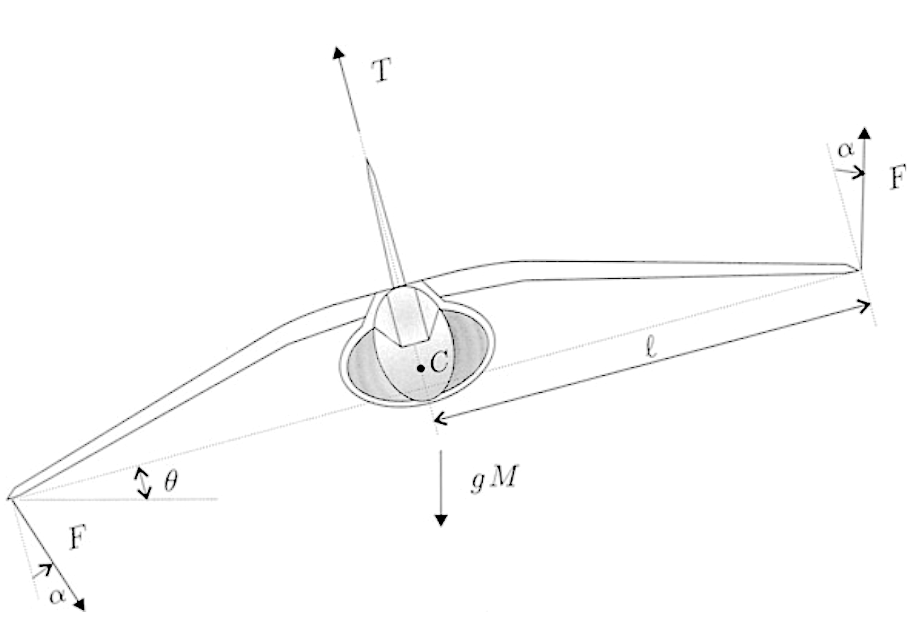
Figure 1: The vertical takeoff and landing aircraft considered in numerical simulations.

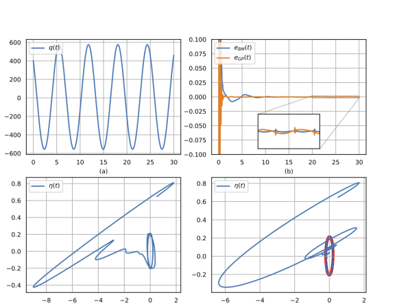
Figure 2: Results obtained comparing our approach $(e_{GP})$ versus [1] $(e_{BM})$ when the exogenous disturbance $d(w)$ is generated by (18). In both cases, the used regulator parameters are the same reported in Table II. In the figure, image $(a)$ depicts the injected noise, $(b)$ compares the behavior of the regulation errors, while $(c)$ and $(d)$ shows the dynamics of $(\eta_{1},\eta_{2})$ along the experiments in which the Bin-Marconi regulator [1] and ours is applied, respectively. In figure $(c)$ the used samples $(\varsigma)$ during the last flow interval are shown as red dots.

We consider, as a testbed, the problem of regulation the lateral $\left(y_{1},y_{2}\right)$ and angular $\left(\theta_{1},\theta_{2}\right)$ dynamics of a Vertical-TakeOff-and-Landing (VTOL) aircraft [36] subjected to lateral forces produced by the wind denoted by $d(w)$. A graphical representation of the considered system is reported in Figure 1. The VTOL dynamics reads as

$$\begin{matrix}\begin{split}\dot{y}_{1}&=y_{2},\\ \dot{y}_{2}&=d(w)-\boldsymbol{g}\tan(\theta_{1})+v,\end{split}&\begin{split}\dot{\theta}_{1}&=\theta_{2},\\ \dot{\theta}_{2}&=2\boldsymbol{l}J^{-1}u,\end{split}\end{matrix}$$ (16)

where $M>0$ and $J>0$ are the aircraft mass and inertia respectively, while $\boldsymbol{l}>0$ represents the wings lenght and $\boldsymbol{g}>0$ the gravitational constant. The input $u$ is the force $\left(F\right)$ on the wingtips, $v$ is a vanishing input taking into account the (controlled) vertical dynamics (not considered here), and $d(w):=M^{-1}d_{0}(w)$, with $d_{0}(w)$ that is the lateral force produced by the wind. Considering as regulation error the aircraft lateral position $\left(e=y_{1}\right)$, the control objective is to remove the wind disturbance out from the lateral dynamics. Let $w(t)$ be generated by an exosystem of the form (2) and consider the following change of coordinates

$$\begin{matrix}\begin{split}\chi_{1}&=y_{1},\\ \chi_{2}&=y_{2},\end{split}&\begin{split}\chi_{3}&=d(w)+\boldsymbol{g}\tan(\theta_{1}),\\ \zeta&=L_{s}d(w)-{\boldsymbol{g}\theta_{2}}/{\cos(\theta_{1})}.\end{split}\end{matrix}$$

In the new coordinates, letting $x=\text{col}(\chi,\zeta)$, the system (16) reads as follow

$$\begin{matrix}\begin{split}\dot{\chi}_{1}&=\chi_{2},\\ \dot{\chi}_{2}&=\chi_{3},\end{split}&\begin{split}\dot{\chi}_{3}&=\zeta,\\ \dot{\zeta}&=q(w,x)+\Omega(w,x)u,\end{split}\end{matrix}$$ (17)

with $q(w,x)$ and $\Omega(w,x)$ given by

$$\begin{split}q(w,x)=L_{s}^{2}d(w)-&\frac{1}{\boldsymbol{g}}\left(L_{s}d(w)-\zeta\right)^{2}\\ &\sin\left(2\tan^{-1}\left(\frac{d(w)-\chi_{3}}{\boldsymbol{g}}\right)\right),\end{split}$$

$$\Omega(w,x)=-2\boldsymbol{g}\boldsymbol{l}J^{-1}\cos\left(\tan^{-1}\left(\frac{d(w)-\chi_{3}}{\boldsymbol{g}}\right)\right)^{-2}.$$

The system (17) is in the form (3) with Assumption II.1 trivially fulfilled, since the $x_{0}$ dynamics is absent, by $x^{*}=0$ and $u^{*}=\left(\boldsymbol{g}L_{s}^{2}d(w)-2d(w)(\boldsymbol{g}^{2}+d(w)^{2})(L_{s}d(w))^{2}\right)/2\boldsymbol{l}J^{-1}(\boldsymbol{g}^{2}+d(w)^{2})$, and Assumption II.2 fulfilled on each compact set with $\mathcal{L}$ a negative number. With $\left(c_{1},c_{2},c_{3}\right)$ the coefficients of a Hurwitz polynomial and $\delta,l>0$ design parameters, we fix the control law as

$$\begin{split}u=\mathcal{L}\Big{[}c_{1}&l\delta^{3}(y_{1}+\eta_{1})+c_{2}l\delta^{2}y_{2}\\ &+c_{3}l\delta(-\boldsymbol{g}\tan(\theta_{1}))+l(-\boldsymbol{g}\theta_{2}/\cos^{2}(\theta_{1}))\Big{]}.\end{split}$$

Figures 2, 3, and 4 report the obtained results when the aircraft is perturbed with a lateral disturbance $d(w)=(2(10^{7}w_{1})+10^{6}w_{3})/M$, where $w_{1}$ and $w_{3}$ are the states of three different exosystems. In particular, in Figure 2, $s(w)$ reads as

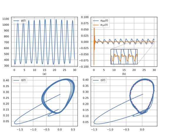
Figure 3: Results obtained comaring our approach $(e_{GP})$ versus [1] $(e_{BM})$ when the exogenous disturbance $d(w)$ is generated by (19). For a comprehensive explanation of Figures $(a)$, $(b)$, $(c)$, and $(d)$ please refer to Figure 2

$$\begin{matrix}\begin{split}\dot{w}_{1}&=w_{2},\\ \dot{w}_{2}&=-w_{1},\\ \end{split}&\begin{split}\dot{w}_{3}&=w_{4},\\ \dot{w}_{4}&=-4w_{3},\end{split}\end{matrix}$$ (18)

in Figure 3, $s(w)$ behaves as

$$\begin{matrix}\begin{split}\dot{w}_{1}&=w_{2},\\ \dot{w}_{2}&=4w_{1}-w_{1}^{3},\\ \end{split}&\begin{split}\dot{w}_{3}&=w_{4},\\ \dot{w}_{4}&=-4w_{3},\end{split}\end{matrix}$$ (19)

while in Figure 4, the exosystem is described by

$$\begin{matrix}\begin{split}\dot{w}_{1}&=w_{2},\\ \dot{w}_{2}&=3\tan^{-1}\left(w_{1}\right)-w_{1},\\ \end{split}&\begin{split}\dot{w}_{3}&=w_{4},\\ \dot{w}_{4}&=-4w_{3}.\end{split}\end{matrix}$$ (20)

In all simulations we exploit the same set of parameters, for both the regulator and the discrete-time identifier. The adopted parameters are reported in Table I, Table II, and Table III.

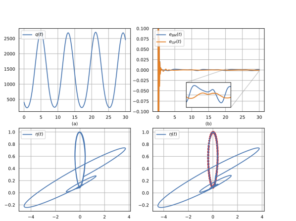
Figure 4: Results obtained comaring our approach $(e_{GP})$ versus [1] $(e_{BM})$ when the exogenous disturbance $d(w)$ is generated by (20). For a comprehensive explanation of Figures $(a)$, $(b)$, $(c)$, and $(d)$ please refer to Figure 2

$n_{\text{ds}}$	$\lambda_{\eta_{1}}$	$\lambda_{\eta_{2}}$	$\lambda_{\tau}$	$\sigma^{2}_{p}$	$\sigma^{2}_{n}$	$\sigma^{2}_{\text{thr}}$
$100$	$0.1$	$0.1$	$2$	$1$	$0.01$	$0.1$

TABLE I: Gaussian process parameters used in simulations.

$\left(c_{1},c_{2},c_{3}\right)$	$l$	$\delta$	$\mathcal{L}$	$\left(h_{1},h_{2}\right)$	$g$	$\left(m_{1},m_{2}\right)$	$\rho$
$\left(15,75,125\right)$	$250$	$150$	$20$	$\left(15,70\right)$	$2$	$\left(20,20\right)$	$2$

TABLE II: Regulator parameters used in simulations.

$M$	$J$	$\boldsymbol{l}$	$\boldsymbol{g}$
$5\cdot 10^{4}$	$1.25\cdot 10^{4}$	$2$	$9.81$

TABLE III: Model parameters used in simulations.

V Conclusions

We presented an adaptive learninm-based technique to design internal model-based regulator for a large class of nonlinear systems. The technique fits in the general framework recently proposed in [1] and shows how the identification of the optimal steady state control input can be performed by using Gaussian process models. As opposite to previous approaches no immersion assumptions into specific model sets are assumed and only smoothness of the ideal steady state control input is required. The learning-based adaptation is performed by following an “event-triggered” logic and hybrid tools are used in the analysis of the closed-loop system. The paper also presents numerical simulations showing how the proposed method outperforms previous approaches when the regulated plant or the exogenous disturbances are subject to unmodeled perturbations.

References

- [1] M. Bin and L. Marconi. “class-type” identification-based internal models in multivariable nonlinear output regulation. IEEE Transactions on Automatic Control, 65(10):4369–4376, 2019.
- [2] B. A. Francis and W. M. Wonham. The internal model principle of control theory. Automatica, 12(5):457–465, 1976.
- [3] E. Davison. The robust control of a servomechanism problem for linear time-invariant multivariable systems. IEEE transactions on Automatic Control, 21(1):25–34, 1976.
- [4] C. I. Byrnes, F. D. Priscoli, A. Isidori, and W. Kang. Structurally stable output regulation of nonlinear systems. Automatica, 33(3):369–385, 1997.
- [5] A. Isidori and C. I. Byrnes. Output regulation of nonlinear systems. IEEE transactions on Automatic Control, 35(2):131–140, 1990.
- [6] C. I. Byrnes and A. Isidori. Limit sets, zero dynamics, and internal models in the problem of nonlinear output regulation. IEEE Transactions on Automatic Control, 48(10):1712–1723, 2003.
- [7] L. Marconi, L. Praly, and A. Isidori. Output stabilization via nonlinear luenberger observers. SIAM Journal on Control and Optimization, 45(6):2277–2298, 2007.
- [8] C.I. Byrnes, A. Isidori, and L. Praly. On the asymptotic properties of a system arising in non-equilibrium theory of output regulation. Preprint of the Mittag-Leffler Institute, Stockholm, 18:2002–2003, 2003.
- [9] L. Wang, A. Isidori, H. Su, and L. Marconi. Nonlinear output regulation for invertible nonlinear mimo systems. International Journal of Robust and Nonlinear Control, 26(11):2401–2417, 2016.
- [10] L. Wang, A. Isidori, Z. Liu, and H. Su. Robust output regulation for invertible nonlinear mimo systems. Automatica, 82:278–286, 2017.
- [11] M. Bin, D. Astolfi, L. Marconi, and L. Praly. About robustness of internal model-based control for linear and nonlinear systems. In 2018 IEEE Conference on Decision and Control (CDC), pages 5397–5402. IEEE, 2018.
- [12] L. Marconi and L. Praly. Uniform practical nonlinear output regulation. IEEE Transactions on Automatic Control, 53(5):1184–1202, 2008.
- [13] D. Astolfi, L. Praly, and L. Marconi. Approximate regulation for nonlinear systems in presence of periodic disturbances. In 2015 54th IEEE Conference on Decision and Control (CDC), pages 7665–7670. IEEE, 2015.
- [14] A. Isidori, L. Marconi, and L. Praly. Robust design of nonlinear internal models without adaptation. Automatica, 48(10):2409–2419, 2012.
- [15] L. B. Freidovich and H. K. Khalil. Performance recovery of feedback-linearization-based designs. IEEE Transactions on automatic control, 53(10):2324–2334, 2008.
- [16] F. D. Priscoli, L. Marconi, and A. Isidori. A new approach to adaptive nonlinear regulation. SIAM Journal on Control and Optimization, 45(3):829–855, 2006.
- [17] A. Pyrkin and A. Isidori. Output regulation for robustly minimum-phase multivariable nonlinear systems. In 2017 IEEE 56th Annual Conference on Decision and Control (CDC), pages 873–878. IEEE, 2017.
- [18] M. Bin, L. Marconi, and A. R. Teel. Adaptive output regulation for linear systems via discrete-time identifiers. Automatica, 105:422–432, 2019.
- [19] F. Forte, L. Marconi, and A. R. Teel. Robust nonlinear regulation: Continuous-time internal models and hybrid identifiers. IEEE Transactions on Automatic Control, 62(7):3136–3151, 2016.
- [20] M. Bin, P. Bernard, and L. Marconi. Approximate nonlinear regulation via identification-based adaptive internal models. IEEE Transactions on Automatic Control, 66(8):3534–3549, 2020.
- [21] J. Kocijan. Modelling and control of dynamic systems using Gaussian process models. Springer, 2016.
- [22] M. Buisson-Fenet, F. Solowjow, and S. Trimpe. Actively learning gaussian process dynamics. In Learning for dynamics and control, pages 5–15. PMLR, 2020.
- [23] C. E. Rasmussen. Gaussian processes in machine learning. In Summer school on machine learning, pages 63–71. Springer, 2003.
- [24] J. Umlauft and S. Hirche. Learning stochastically stable gaussian process state–space models. IFAC Journal of Systems and Control, 12:100079, 2020.
- [25] A. Lederer, J. Umlauft, and S. Hirche. Uniform error bounds for gaussian process regression with application to safe control. Advances in Neural Information Processing Systems, 32, 2019.
- [26] L. Sforni, I. Notarnicola, and G. Notarstefano. Learning-driven nonlinear optimal control via gaussian process regression. In 2021 60th IEEE Conference on Decision and Control (CDC), pages 4412–4417. IEEE, 2021.
- [27] G. Torrente, E. Kaufmann, P. Föhn, and D. Scaramuzza. Data-driven mpc for quadrotors. IEEE Robotics and Automation Letters, 6(2):3769–3776, 2021.
- [28] J. Kabzan, L. Hewing, A. Liniger, and M. N. Zeilinger. Learning-based model predictive control for autonomous racing. IEEE Robotics and Automation Letters, 4(4):3363–3370, 2019.
- [29] M. Buisson-Fenet, V. Morgenthaler, S. Trimpe, and F. Di Meglio. Joint state and dynamics estimation with high-gain observers and gaussian process models. In 2021 American Control Conference (ACC), pages 4027–4032. IEEE, 2021.
- [30] M. Bin and L. Marconi. The chicken-egg dilemma and the robustness issue in nonlinear output regulation with a look towards adaptation and universal approximators. In 2018 IEEE Conference on Decision and Control (CDC), pages 5391–5396. IEEE, 2018.
- [31] L. Wang, A. Isidori, and H. Su. Global stabilization of a class of invertible mimo nonlinear systems. IEEE Transactions on Automatic Control, 60(3):616–631, 2014.
- [32] F. O’sullivan, B. S. Yandell, and W. J. Raynor Jr. Automatic smoothing of regression functions in generalized linear models. Journal of the American Statistical Association, 81(393):96–103, 1986.
- [33] J. P. Hespanha and A. S. Morse. Stability of switched systems with average dwell-time. In Proceedings of the 38th IEEE conference on decision and control (Cat. No. 99CH36304), volume 3, pages 2655–2660. IEEE, 1999.
- [34] J. P. Hespanha, D. Liberzon, and A. R. Teel. On input-to-state stability of impulsive systems. In Proceedings of the 44th IEEE Conference on Decision and Control, pages 3992–3997. IEEE, 2005.
- [35] A. Lederer, J. Umlauft, and S. Hirche. Uniform error and posterior variance bounds for gaussian process regression with application to safe control. arXiv preprint arXiv:2101.05328, 2021.
- [36] A. Isidori, L. Marconi, and A. Serrani. Robust autonomous guidance: an internal model approach. Springer Science & Business Media, 2003.