Optimal dividends under a drawdown constraint
and a curious square-root rule

Abstract

In this paper we address the problem of optimal dividend payout strategies from a surplus process governed by Brownian motion with drift under a drawdown constraint, i.e. the dividend rate can never decrease below a given fraction $a$ of its historical maximum. We solve the resulting two-dimensional optimal control problem and identify the value function as the unique viscosity solution of the corresponding Hamilton-Jacobi-Bellman equation. We then derive sufficient conditions under which a two-curve strategy is optimal, and show how to determine its concrete form using calculus of variations. We establish a smooth-pasting principle and show how it can be used to prove the optimality of two-curve strategies for sufficiently large initial and maximum dividend rate. We also give a number of numerical illustrations in which the optimality of the two-curve strategy can be established for instances with smaller values of the maximum dividend rate, and the concrete form of the curves can be determined. One observes that the resulting drawdown strategies nicely interpolate between the solution for the classical unconstrained dividend problem and the one for a ratcheting constraint as recently studied in [1]. When the maximum allowed dividend rate tends to infinity, we show a surprisingly simple and somewhat intriguing limit result in terms of the parameter $a$ for the surplus level on from which, for sufficiently large current dividend rate, a take-the-money-and-run strategy is optimal in the presence of the drawdown constraint.

1 Introduction and model

Assume that the surplus process of a company is given by a Brownian motion with drift

$$X_{t}=x+\mu t+\sigma W_{t},$$ (1.1)

where $W_{t}$ is a standard Brownian motion, and $\mu,\sigma>0$ are given constants. Let $(\Omega,\mathcal{F},\left(\mathcal{F}_{t}\right)_{t\geq 0},\mathcal{P})$ be the complete probability space generated by the process $X_{t}$. Assume further that the company uses part of the surplus to pay dividends to the shareholders with rates in a set $[0,\overline{c}]$, where $\overline{c}>0$ is the maximum dividend rate possible. Let $D_{t}$ denote the rate at which the company pays dividends at time $t$, then the controlled surplus process can be written as

$$X_{t}^{D}=X_{t}-\int_{0}^{t}D_{s}ds.$$ (1.2)

It is a classical problem in risk theory to find the dividend strategy $D=\left(D_{t}\right)_{t\geq 0}$ that maximizes the expected sum of discounted dividend payments

$$J(x;D)=\mathbb{E}\left[\int_{0}^{\tau}e^{-qs}D_{s}ds\right]$$ (1.3)

over a set of admissible candidate strategies. Here $q>0$ is a discount factor and $\tau=\inf\left\{t\geq 0:X_{t}^{D}<0\right\}$ is the ruin time of the controlled process. De Finetti [15] was the first to consider a problem of this kind for a simple random walk, and Gerber [19, 20] considered extensions, including the diffusion setup (1.1) given above. For a finite maximum dividend rate $\overline{c}$, this problem was then further investigated by Shreve et al. [29], Jeanblanc and Shiryaev [23], Radner and Shepp [27], Asmussen and Taksar [7] and Gerber and Shiu [21]. Since then, a lot of variants of this problem for the process (1.1) and more general underlying risk processes have been considered, see e.g. the surveys [4] and [8].
For the diffusion model (1.1), in [1] we recently studied this optimal dividend problem under a ratcheting constraint, i.e. under the assumption that the dividend rate can never be decreased over the lifetime of the process, which renders the respective control problem two-dimensional, where the first dimension is the current surplus and the second dimension is the currently employed dividend rate. One motivation to consider that constraint was that it may be psychologically preferable to shareholders to not experience a decrease of dividend payments, and it is interesting to see to what extent such a constraint leads to an overall performance loss.

In this paper we would like to go one step further and allow reductions of the dividend rate over time, but only up to a certain percentage $a$ of the largest already exercised dividend rate (”drawdown”). More formally, a dividend drawdown strategy $D=\left(D_{t}\right)_{t\geq 0}$ with drawdown constraint $a\in[0,1]$ is one that satisfies $D_{t}\in[aR_{t},\overline{c}]$, where $R_{t}$ is the running maximum of the dividend rates, that is

$$R_{t}:=\max\{D_{s}:0\leq s\leq t\}\vee c;$$

here we denote the initial dividend rate by $R_{0^{-}}=c$. A dividend drawdown strategy is called admissible if it is right-continuous and adapted with respect to the filtration $\left(\mathcal{F}_{t}\right)_{t\geq 0}.$

Define $\Pi_{x,c,a}^{[0,\overline{c}]}$ as the set of all admissible dividend drawdown strategies with initial surplus $x\geq 0$, initial running maximum dividend rate $c\in[0,\overline{c}]$ and drawdown constraint $a\in[0,1]$. Given $D\in\Pi_{x,c,a}^{[0,\overline{c}]}$, the value function of this strategy is given by (1.3). Hence, for any initial surplus $x\geq 0$, initial running maximum dividend rate $c\in[0,\overline{c}]$ and drawdown constraint $a\in[0,1]$, our aim in this paper is to maximize

$$V_{a}^{\overline{c}}(x,c)=\sup_{D\in\Pi_{x,c,a}^{[0,\overline{c}]}}J(x;D).$$ (1.4)

Note that the limit case $a=1$ corresponds to the ratcheting case (considered previously in [1]) and the limit case $a=0$ corresponds to the optimization of bounded dividend rates without any drawdown constraint.

Drawdown phenomena have been studied in various contexts in the literature. On the one hand, drawdown times and properties of uncontrolled stochastic processes were investigated in quite some generality (see for instance Landriault et al. [25] for the case of Lévy processes). In the context of control problems, drawdown constraints on the wealth have been considered in portfolio problems in the mathematical finance literature, see for instance Elie and Touzi [18], Chen et al. [14] and Kardaras et al. [24]. For a minimization of drawdown times of a risk process through dynamic reinsurance, see Brinker [11] and Brinker and Schmidli [12]. Our context, however, is different, as we are interested in implementing a drawdown constraint on the payment structure of the dividend rates, i.e., as a constraint on the admissible dividend policies. In that sense, our approach is closer related to problems of lifetime consumption in the mathematical finance literature, see Angoshtari et al. [5] who extend the Dusenberry’s ratcheting problem of consumption studied by Dybvig [16] to drawdown constraints. However, the concrete model setup and embedding, and also the involved techniques there are very different from dividend problems of the De Finetti-type as studied in this paper.

After deriving some basic analytic properties of the value function $V_{a}^{\overline{c}}(x,c)$ of our drawdown problem in Section 3, we will derive a Hamilton-Jacobi-Bellman equation for $V_{a}^{\overline{c}}(x,c)$ in Section 4 and show that $V_{a}^{\overline{c}}(x,c)$ is its unique viscosity solution with suitable boundary condition. We then, in Section 5, briefly study in more detail the value function when one already starts at the maximal dividend rate $\overline{c}$, which serves as a crucial ingredient in the derivation of $V_{a}^{\overline{c}}(x,c)$ in Section 6. Sufficient conditions are given under which the optimal strategy for bounded dividend rates is a two-curve strategy in the space $(x,c)\in(0,\infty)\times[0,\overline{c}]$, which is partitioned by two curves $\gamma^{\overline{c}}(c)$ and $\zeta^{\overline{c}}(c)$, with $\gamma^{\overline{c}}(c)<\zeta^{\overline{c}}(c)$ for all $c\in[0,\overline{c}]$: if for a given $c$, $x<\gamma^{\overline{c}}(c)$, then dividends are paid at rate $ac$; if $\gamma^{\overline{c}}(c)\leq x\leq\zeta^{\overline{c}}(c)$, then dividends are paid at rate $c$; finally, if $x>\zeta^{\overline{c}}(c)$, then the dividend rate $c$ is increased immediately until $x=\zeta^{\overline{c}}(c_{1})$ for some $c_{1}\in(c,\overline{c})$ (or $c=\overline{c}$, whichever happens first) is reached. We furthermore establish a smooth-pasting principle for these optimal curves. In Section 7 it is shown that the limits of $\gamma^{\overline{c}}(\overline{c})$ and $\zeta^{\overline{c}}(\overline{c})$ as $\overline{c}\rightarrow\infty$ are finite, and given by surprisingly explicit formulas:

$$\lim_{\overline{c}\rightarrow\infty}\gamma^{\overline{c}}(\overline{c})=\frac{\mu}{q}\quad\text{and}\quad\lim_{\overline{c}\rightarrow\infty}\zeta^{\overline{c}}(\overline{c})=\frac{\mu}{q}{\hbox{$\left(\vbox to0.0pt{}\right.\n@space$}}1+\frac{1}{\sqrt{a}}{\hbox{$\left)\vbox to0.0pt{}\right.\n@space$}}.$$ (1.5)

This nicely extends the respective limit $2\mu/q$ of the ratcheting curve that was identified for pure ratcheting ($a=1$) in [1, Lem.5.21].
In Section 8 we then look further into the limiting case, and show that for sufficiently large $\overline{c}$, one has $\gamma^{\overline{c}}(c)\nearrow\gamma^{\overline{c}}(\overline{c})$ and $\zeta^{\overline{c}}(c)\searrow\zeta^{\overline{c}}(\overline{c})$ as $c\to\overline{c}$. This enables to establish the general optimality of two-curve strategies whenever the current dividend rate $c$ and the maximal dividend rate $\overline{c}$ are sufficiently large. At the same time, the negative derivative of $\zeta^{\overline{c}}(c)$ close to (sufficiently large) $\overline{c}$ is notably different from the pure ratcheting case ($a=1$) for which it was shown in [1] that the corresponding derivative is positive for all $c$ close to $\overline{c}$ (and indeed the leading term in the asymptotics of $0<a<1$ breaks down for $a=1$ so that some sort of phase transition happens). The simplicity of the right-hand limit in (1.5) and in particular the appearance of the square-root of the drawdown coefficient $a$ in the right-hand limit are somewhat intriguing. In the absence of an upper limit for the dividend rate, it identifies the minimum surplus level $x$ on from which, for sufficiently large current dividend rate, it is preferable to pay out all the surplus $x$ immediately and generate ruin by doing so (a so-called ”take-the-money-and-run”-strategy, see e.g. [26]), and that value does not depend on the size of the volatility $\sigma$. Consequently, one can get some intuition on its nature in the much simpler deterministic model with $\sigma=0$, which we will therefore consider in Section 2 before approaching the general case $\sigma>0$ in the rest of the paper.
We give numerical illustrations in Section 9, where we establish the optimality of two-curve strategies also for smaller magnitudes of $c$ and $\overline{c}$ by numerically showing that the sufficient conditions from Section 6 are satisfied. We obtain the optimal curves by calculus of variation techniques and discuss the properties of the value functions of the drawdown dividend problem and their comparison to classical and ratcheting solutions for various parameter combinations. Finally, Section 10 concludes, and Section 11 collects some longer formulas appearing in the paper in a compact form.

2 Some intuition from the deterministic case

Assume in this section for simplicity a completely deterministic model

$$X_{t}=x+\mu t$$

with a positive drift $\mu>0$ (for the study of such a model in another context in the dividend literature, see e.g. [17]). Then a constant dividend rate $\overline{c}=\mu$ throughout time will keep the surplus at level $x$ for all $t\geq 0$ and correspondingly

$$\mathbb{E}\left[\int_{0}^{\tau}e^{-qs}D_{s}ds\right]=\mathbb{E}\left[\int_{0}^{\infty}e^{-qs}\mu\,ds\right]=\frac{\mu}{q}$$

for any $x>0$. Consequently, whenever the initial surplus $x$ is larger than $\mu/\delta$, paying out all the surplus at the beginning (causing immediate ruin) will be preferable to any other dividend strategy subject to the constraint $\overline{c}\leq\mu$.
At the same time, if a constant dividend rate $\overline{c}>\mu$ is applied, the controlled process will lead to ruin at time $t=x/(\overline{c}-\mu)$ and we obtain instead

$$\mathbb{E}\left[\int_{0}^{\tau}e^{-qs}D_{s}ds\right] =\mathbb{E}\left[\int_{0}^{x/(\overline{c}-\mu)}e^{-qs}\overline{c}\,ds\right]=\frac{\overline{c}}{q}\left(1-e^{-qx/(\overline{c}-\mu)}\right)$$

$$=x+x\,\frac{2\mu-qx}{2\overline{c}}+O\left(\frac{1}{\overline{c}^{2}}\right).$$

The latter shows that whenever $x>2\mu/q$, if allowed to do so, paying out all the surplus $x$ immediately (and causing immediate ruin) will be preferable to any other constant dividend strategy with large $\overline{c}$. In other words, the potential gain from later ruin and therefore more dividend income (by exploiting the positive drift, without any risk) is outweighed by the discounting of such later dividend payments. This can also be seen as an intuitive explanation of the limit $2\mu/q$ in [1, Lem.5.21].

Let us now proceed to the case with drawdown: Assume that we start with initial capital $x>b$ for some $b$ to be determined and that we pay dividends at rate $\overline{c}>\mu$ until we reach that lower level $b$ at time $t=(x-b)/(\overline{c}-\mu)$, from which time on we reduce the dividend payments to level $a\cdot\overline{c}$ according to our drawdown constraint. In the deterministic model of this section, this then leads to

$$\mathbb{E}\left[\int_{0}^{\tau}e^{-qs}D_{s}ds\right] =\frac{\overline{c}}{q}\left(1-e^{-q\frac{x-b}{\overline{c}-\mu}}\right)+e^{-q\frac{x-b}{\overline{c}-\mu}}\cdot\frac{a\,\overline{c}}{q}\,\left(1-e^{-q\frac{b}{a\overline{c}-\mu}}\right).$$ (2.1)

Taking the derivative with respect to $b$ and setting it zero gives, after simple calculations, for large $\overline{c}$, the optimal level

$$b^{*}(\overline{c}) =\frac{a\overline{c}-\mu}{q}\log\left(\frac{a\overline{c}}{a\overline{c}-\mu}\right)$$ (2.2)

$$=\frac{\mu}{q}-\frac{\mu^{2}}{2aq\overline{c}}+O\left(\frac{1}{\overline{c}^{2}}\right).$$

But if one substitutes that value of $b$ into (2.1), then an expansion at $\overline{c}=\infty$ gives

$$\mathbb{E}\left[\int_{0}^{\tau}e^{-qs}D_{s}ds\right] =x+\frac{2axq\mu-ax^{2}q^{2}+\mu^{2}(1-a)}{2aq\,\overline{c}}+O\left(\frac{1}{\overline{c}^{2}}\right).$$ (2.3)

The numerator in the second term is negative exactly when

$$x>\frac{\mu}{q}{\hbox{$\left(\vbox to0.0pt{}\right.\n@space$}}1+\frac{1}{\sqrt{a}}{\hbox{$\left)\vbox to0.0pt{}\right.\n@space$}},$$

so that in those cases it is preferable to immediately pay $x$ as a lump sum dividend and go to ruin immediately (if that is allowed) rather than following the above refracting strategy, as the value $x$ can not be realized at any later point in time in view of the discounting, despite the continuing deterministic income with drift $\mu$.
One may expect that the size of the volatility does not matter when $\overline{c}\to\infty$, and indeed, as a by-product of the results of this paper, it will be shown in Section 7 that the same limit can be established for the general case $\sigma>0$, cf. Proposition 7.3. Another way to state this is the following: if one defines $x^{*}(\overline{c})$ as the surplus value for which, when already currently paying the maximum dividend rate $\overline{c}$, one is indifferent whether to further increase the dividend rate or not, then the above result establishes that $\lim_{\overline{c}\to\infty}x^{*}(\overline{c})=\frac{\mu}{q}(1+{1}/\sqrt{a})$, and it will be in terms of that notation that the more general result is proved in Section 7.

3 Basic results

Recall the definition of our optimal value function $V_{a}^{\overline{c}}(x,c)$ (1.4) and denote by $V_{a}^{\infty}(x,c)$ the corresponding function when there is no ceiling on dividend rates, i.e. $\overline{c}=\infty$. It is immediate to see that $V_{a}^{\overline{c}}(0,c)=0$ for all $c\in[0,\overline{c}]$ and $a\in[0,1]$.

Remark 3.1

As mentioned in the introduction, the dividend optimization problem without drawdown constraint has a long history and, for a finite $\overline{c}$ and the diffusion setup, was first addressed in Shreve et al. [29]. Unlike the drawdown optimization problem, the problem without the drawdown constraint is one-dimensional. If we denote its optimal value function by $\overline{V}^{\overline{c}}(x),$ then clearly $V_{0}^{\overline{c}}(x,c)=\overline{V}^{\overline{c}}(x)$ and $V_{a}^{\overline{c}}(x,c)\leq\overline{V}^{\overline{c}}(x)$ for all $x\geq 0$, $a\in[0,1]$ and $c\in[0,\overline{c}]$. The function $\overline{V}^{\overline{c}}$ is increasing, concave, twice continuously differentiable with $\overline{V}^{\overline{c}}(0)=0$ and $\lim_{x\rightarrow\infty}\overline{V}^{\overline{c}}(x)=\overline{c}/q$; so it is Lipschitz with Lipschitz constant $\left(\overline{V}^{\overline{c}}\right)^{\prime}(0).$

Remark 3.2

The dividend optimization problem without any constraint was addressed by Gerber and Shiu [21] and Schmidli [28]. If $\overline{V}(x)$ denotes its optimal value function, we have $\overline{V}(x)=V_{0}^{\infty}(x,c)$ for any $c>0$. Clearly $V_{a}^{\infty}(x,c)\leq\overline{V}(x)$ for all $a\in[0,1]$. The function $\overline{V}$ is increasing, concave, twice continuously differentiable with $\overline{V}(0)=0$ and $x\leq\overline{V}(x)\leq x+\mu/q$; so it is Lipschitz with Lipschitz constant $\overline{V}^{\prime}(0)$.

Proposition 3.1

It holds that $V_{a}^{\overline{c}}(x,c)\nearrow V_{a}^{\infty}(x,c)$ as $\overline{c}\rightarrow\infty.$

Proof. It is straightforward that for any $\overline{c}_{1}\leq$ $\overline{c}_{2}$, $V_{a}^{\overline{c}_{1}}(x,c)\leq V_{a}^{\overline{c}_{2}}(x,c)$ $\leq V_{a}^{\infty}(x,c)$ for $0\leq c\leq\overline{c}_{1}$. Take for any $\varepsilon>0,$ a strategy $D=(D_{t})_{t\geq 0}\in\Pi_{x,c,a}^{[0,\infty)}$ with ruin time $\tau$, such that $V_{a}^{\infty}(x,c)\leq J(x;D)+\varepsilon$. Let us consider for an increasing sequence with $c_{n}\rightarrow\infty$ and $c_{1}>c$, $D^{n}=(D_{t}\wedge c_{n})_{t\geq 0}\in\Pi_{x,c,a}^{[0,c_{n})}$ and let $\tau^{n}\geq\tau$ be the ruin time of $D^{n}$. Then, by the theorem of monotone convergence,

$$\lim_{n\rightarrow\infty}J(x;D_{t}^{n})=\lim_{n\rightarrow\infty}\mathbb{E}\left[\int_{0}^{\tau^{n}}e^{-qs}D_{s}^{n}ds\right]\geq\lim_{n\rightarrow\infty}\mathbb{E}\left[\int_{0}^{\tau}e^{-qs}D_{s}^{n}ds\right]=J(x;D)$$

and so we have the result. $\blacksquare$

We now state a straightforward result regarding the boundedness and monotonicity of the optimal value functions.

Proposition 3.2

In the case $\overline{c}<\infty$, the optimal value function $V_{a}^{\overline{c}}(x,c)$ is bounded by $\overline{c}/q$ with $\lim_{x\rightarrow\infty}V_{a}^{\overline{c}}(x)=\overline{c}/q$, non-decreasing in $x$ and non-increasing in $c$.

Proof. By Remark 3.1 and Theorem 3.3 of [1], we have that

$$V_{1}^{\overline{c}}(x,c)\leq V_{a}^{\overline{c}}(x,c)\leq\overline{V}^{\overline{c}}(x)$$

with $\lim_{x\rightarrow\infty}V_{1}^{\overline{c}}(x,c)=\lim_{x\rightarrow\infty}\overline{V}^{\overline{c}}(x)=\overline{c}/q,$ so $V_{a}^{\overline{c}}$ is bounded by $\overline{c}/q$ with $\lim_{x\rightarrow\infty}V_{a}^{\overline{c}}(x,c)=\overline{c}/q.$

On the one hand $V_{a}^{\overline{c}}(x,c)$ is non-increasing in $c$ because given $c_{1}<c_{2}\leq\overline{c},$ we have $\Pi_{x,c_{2},a}^{[0,\overline{c}]}\subset\Pi_{x,c_{1,a}}^{[0,\overline{c}]}$ for any $x\geq 0$. On the other hand, given $0\leq x_{1}<x_{2}$ and an admissible ratcheting strategy $D_{1}\in\Pi_{x_{1},c,a}^{[0,\overline{c}]}$ for any $c\in[0,\overline{c}]$, let us define $D_{2}\in\Pi_{x_{2},c,a}^{[0,\overline{c}]}$ as $D_{2,t}=D_{1.t}$ until the ruin time of the controlled process $X_{t}^{D^{1}}$ with $X_{0}^{D^{1}}=x_{1}$, and pay the maximum rate $\overline{c}$ afterwards. Thus, $J(x;D_{1})\leq J(x;D_{2})$ and we have the result. $\blacksquare$

Proposition 3.3

$V_{a}^{\infty}(x,c)$ is non-decreasing in $x$ and non-increasing in $c.$ For the case $a>0,\$we have $\lim_{c\rightarrow\infty}V_{a}^{\infty}(x,c)=x$. Moreover $x\leq V_{a}^{\infty}(x,c)\leq x+\mu/q.$

Proof. By Propositions 3.1 and 3.2, we have that $V_{a}^{\infty}(x,c)$ is non-decreasing in $x$ and non-increasing in $c$. Let us show now that $V_{a}^{\infty}(x,c)\geq x$. The function $V_{a}^{\infty}(x,c)$ is bounded from below by the expected discounted dividends resulting from the strategy of paying a constant rate $n$ up to ruin. Defining ${\tau}_{n}=\inf\{t:x+(\mu-n)t+\sigma W_{t}=0\}$, one gets

$$V_{a}^{\infty}(x,c)=\lim_{n\rightarrow\infty}V_{a}^{n}(x,c)\geq\lim_{n\rightarrow\infty}\mathbb{E}\left[\int_{0}^{{\tau}_{n}}e^{-qs}\,n\,ds\right]=\lim_{n\rightarrow\infty}\frac{n}{q}(1-\mathbb{E[}e^{-q{\tau}_{n}}])=x,$$

where the last equality follows from Formula 2.0.1 on page 295 of Borodin & Salminen [10].

Finally, let us see that $\lim_{c\rightarrow\infty}V_{a}^{\infty}(x,c)\leq x$. Take for any $\varepsilon>0$ and for each $c$, $D^{c}=(D_{t}^{c})_{t\geq 0}\in\Pi_{x,c,a}^{[0,\infty)}$, such that

$$V_{a}^{\infty}(x,c)\leq J(x;D^{c})+\varepsilon.$$

The corresponding ruin time is then given by

$$\tau^{c}=\inf\left\{t:x+\mu t+\sigma W_{t}-{\textstyle\int\nolimits_{0}^{t}}D_{s}^{c}ds=0\right\}$$

and $D_{s}^{c}\geq ac.$ Hence,

$${\textstyle\int\nolimits_{0}^{\tau^{c}}}D_{s}^{c}ds=x+\mu\tau^{c}+\sigma W_{\tau^{c}}$$

and so

$$\tau^{c}\leq\inf\left\{s:x+(\mu-ac)s+\sigma W_{s}\leq 0\right\}=\inf\left\{s:W_{s}\leq\frac{-x+(ac-\mu)s}{\sigma}\right\}\text{.}$$

Hence, for $c>\mu/a$, $\tau^{c}<\infty$ a.s. and $\mathbb{E}\left[\tau^{c}\right]\rightarrow 0$ as $c\rightarrow\infty$. Therefore,

$$\begin{array}[c]{ll}\lim_{c\rightarrow\infty}\mathbb{E}[{\textstyle\int\nolimits_{0}^{\tau^{c}}}e^{-qs}D_{s}^{c}ds]&\leq\lim_{c\rightarrow\infty}\mathbb{E}[{\textstyle\int\nolimits_{0}^{\tau^{c}}}D_{s}^{c}ds]\\ &=\lim_{c\rightarrow\infty}\mathbb{E}[x+\mu\tau^{c}+\sigma W_{\tau^{c}}]\\ &=x+\mu\lim_{c\rightarrow\infty}\mathbb{E}[\tau^{c}]=x\end{array}$$

and so we have the result. $\blacksquare$

The Lipschitz property of the function $\overline{V}$ can now be used to prove a global Lipschitz result on the regularity of the optimal value function.

Proposition 3.4

In both the restricted case $\overline{c}<\infty$ and the unrestricted case $\overline{c}=\infty,$ we have that

$$0\leq V_{a}^{\overline{c}}(x_{2},c_{1})-V_{a}^{\overline{c}}(x_{1},c_{2})\leq K\left[\left(x_{2}-x_{1}\right)+\left(c_{2}-c_{1}\right)\right]$$

for all $0\leq x_{1}\leq x_{2}$ and $c_{1},c_{2}\in[0,\overline{c}]$ with $c_{1}\leq c_{2}$, with $K=\max\{\frac{e^{-1}}{q}a,1\}\overline{V}^{\prime}(0).$

Proof. In the case $\overline{c}<\infty$, by Proposition 3.2, we have

$$0\leq V_{a}^{\overline{c}}(x_{2},c_{1})-V_{a}^{\overline{c}}(x_{1},c_{2})$$ (3.1)

for all $0\leq x_{1}\leq x_{2}$ and $c_{1},c_{2}\in[0,\overline{c}]$ with $c_{1}\leq c_{2}$.

Let us show now, that there exists $K_{1}>0$ such that

$$V_{a}^{\overline{c}}(x_{2},c)-V_{a}^{\overline{c}}(x_{1},c)\leq K_{1}\left(x_{2}-x_{1}\right)$$ (3.2)

for all $0\leq x_{1}\leq x_{2}$. Take $\varepsilon>0$ and $D\in\Pi_{x_{2},c,a}^{[0,\overline{c}]}$ such that

$$J(x_{2};D)\geq V_{a}^{\overline{c}}(x_{2},c)-\varepsilon,$$ (3.3)

the associated control process is given by

$$X_{t}^{D}=x_{2}+\int_{0}^{t}(\mu-D_{s})ds+\sigma W_{t}.$$

Let $\tau$ be the ruin time of the process $X_{t}^{D}$. Define $\widetilde{D}\in\Pi_{x_{1},c,a}^{[0,\overline{c}]}$ as $\widetilde{D}_{t}=D_{t}$ and the associated control process

$$\text{ }X_{t}^{\widetilde{D}}=x_{1}+\int_{0}^{t}(\mu-D_{s})ds+\sigma W_{t}.$$

Let $\widetilde{\tau}\leq\tau$ be the ruin time of the process $X_{t}^{\widetilde{D}}$; it holds that $X_{t}^{D}-X_{t}^{\widetilde{D}}=x_{2}-x_{1}$ for $t\leq\widetilde{\tau}$.

We can write

$$\begin{array}[c]{lll}J(x_{2};D)-J(x_{1};\widetilde{D})&=&\mathbb{E}\left[\int_{\widetilde{\tau}}^{\tau}e^{-qs}D_{s}ds\right]\\ &=&\mathbb{E}\left[\mathbb{E}\left[\left.\int_{\widetilde{\tau}}^{\tau}e^{-qs}D_{s}ds\right|\mathcal{F}_{\widetilde{\tau}}\right]\right]\\ &=&\mathbb{E}\left[\mathbb{E}\left[\left.e^{-q\widetilde{\tau}}\int_{0}^{\tau-\widetilde{\tau}}e^{-qu}D_{\widetilde{\tau}+u}du\right|\mathcal{F}_{\widetilde{\tau}}\right]\right]\\ &\leq&\mathbb{E}\left[\mathbb{E}\left[\left.\int_{0}^{\tau-\widetilde{\tau}}e^{-qu}D_{\widetilde{\tau}+u}du\right|\mathcal{F}_{\widetilde{\tau}}\right]\right]\\ &\leq&V_{a}^{\overline{c}}(x_{2}-x_{1},0).\end{array}$$ (3.4)

The last inequality of (3.4) involves a shift of stopping times and follows from Theorem 2 of Claisse, Talay and Tan [13]. Indeed, the assumptions of this theorem are satisfied, because we can write our controlled process as

$$dX_{s}=b(s,X,D_{s})ds+\sigma(s,X,D_{s})dW_{s},$$

where $b(s,x,d)=\mu-d$, $\sigma(s,x,d)\equiv\sigma$ and $W_{s}$ is a standard Brownian motion. Hence we have

$$\begin{array}[c]{lll}V_{a}^{\overline{c}}(x_{2},c)-V_{a}^{\overline{c}}(x_{1},c)&\leq&J(x_{2};D)-J(x_{1};\widetilde{D})+\varepsilon\\ &\leq&V^{\overline{c}}(x_{2}-x_{1},0)+\varepsilon\\ &\leq&\overline{V}(x_{2}-x_{1})+\varepsilon\\ &\leq&K_{1}(x_{2}-x_{1})+\varepsilon.\end{array}$$ (3.5)

So, by Remark 3.2, we have (3.2) with $K_{1}=\overline{V}^{\prime}(0).$

Let us show now that, given $c_{1},c_{2}\in[0,\overline{c}]$ with $c_{1}\leq c_{2},$ there exists $K_{2}>0$ such that

$$V_{a}^{\overline{c}}(x,c_{1})-V_{a}^{\overline{c}}(x,c_{2})\leq K_{2}\left(c_{2}-c_{1}\right).$$ (3.6)

Take $\varepsilon>0$ and $D\in\Pi_{x,c_{1,a}}^{[0,\overline{c}]}$ such that

$$J(x;D)\geq V_{a}^{\overline{c}}(x,c_{1})-\varepsilon$$ (3.7)

and denote by $\tau$ the ruin time of the process $X_{t}^{D}$.

Let us consider $\widetilde{D}\in\Pi_{x,c_{2}}^{[0,\overline{c}]}\$as $\widetilde{D}_{t}=\max\{D_{t},ac_{2}\}$; denote by $X_{t}^{\widetilde{D}}$ the associated controlled surplus process and by $\overline{\tau}\leq\tau$ the corresponding ruin time. We have that $\widetilde{D}_{s}-D_{s}\leq ac_{2}-ac_{1}$ and so $X_{\overline{\tau}}^{D}=X_{\overline{\tau}}^{D}-X_{\overline{\tau}}^{\widetilde{D}}\leq a(c_{2}-c_{1})\overline{\tau}$. By Remark 3.2, we have

$$\begin{array}[c]{lll}\mathbb{E}\left[\int_{\overline{\tau}}^{\tau}D_{s}e^{-qs}ds\right]&=&\mathbb{E}\left[\mathbb{E}\left[e^{-q\overline{\tau}}\left.\int_{\overline{\tau}}^{\tau}D_{s}e^{-q\left(s-\overline{\tau}\right)}ds\right|\mathcal{F}_{\overline{\tau}}\right]\right]\\ &\leq&\mathbb{E}\left[\mathbb{E}\left[\left.\int_{0}^{\tau-\overline{\tau}}D_{u+\overline{\tau}}e^{-qu}du\right|\mathcal{F}_{\overline{\tau}}\right]\right]\\ &\leq&\mathbb{E}\left[V_{a}^{\overline{c}}(X_{\overline{\tau}}^{D},0)\right].\end{array}$$

As before, the last inequality involves a shift of stopping times and it follows from Theorem 2 of Claisse, Talay and Tan [13]. Then

$$\begin{array}[c]{lll}\mathbb{E}\left[\int_{\overline{\tau}}^{\tau}D_{s}e^{-qs}ds\right]&\leq&\mathbb{E}\left[\overline{V}(X_{\overline{\tau}}^{D})\right]\\ &\leq&\mathbb{E}\left[\overline{V}((c_{2}-c_{1})\overline{\tau}\right]\\ &\leq&K_{1}\mathbb{E}[e^{-q\overline{\tau}}\overline{\tau}(c_{2}-c_{1})].\end{array}$$

Hence, we can write,

$$\begin{array}[c]{lll}V_{a}^{\overline{c}}(x,c_{1})-V_{a}^{\overline{c}}(x,c_{2})&\leq&J(x;D)+\varepsilon-J(x;\widetilde{D})\\ &=&\mathbb{E}\left[\int_{0}^{\overline{\tau}}\left(D_{s}-\widetilde{D}_{s}\right)e^{-qs}ds\right]+\mathbb{E}\left[\int_{\overline{\tau}}^{\tau}D_{s}e^{-qs}ds\right]+\varepsilon\\ &\leq&0+\mathbb{E}\left[\int_{\overline{\tau}}^{\tau}D_{s}e^{-qs}ds\right]+\varepsilon\\ &\leq&K_{1}E[ae^{-q\overline{\tau}}\overline{\tau}(c_{2}-c_{1})]+\varepsilon\\ &\leq&K_{2}(c_{2}-c_{1})+\varepsilon.\end{array}$$ (3.8)

So, we deduce (3.6), taking $K_{2}=K_{1}\max_{t\geq 0}\{e^{-qt}ta\}=K_{1}\frac{e^{-1}}{q}a\$and $K=K_{1}\max\{\frac{e^{-1}}{q}a,1\}$. We conclude the result from (3.1), (3.2) and (3.6).

In the case $\overline{c}=\infty$, the result follows from Proposition 3.1. $\blacksquare$

The following lemma states the dynamic programming principle, its proof is similar to the one of Lemma 1.2 in Azcue and Muler [9].

Lemma 3.5

Given any stopping time $\widetilde{\tau}$, we can write in both the restricted case $\overline{c}<\infty$ and the unrestricted case $\overline{c}=\infty,$

$$V_{a}^{\overline{c}}(x,c)=\sup\limits_{D\in\Pi_{x,c,a}^{[0,\overline{c}]}}\mathbb{E}\left[\int_{0}^{\tau\wedge\widetilde{\tau}}e^{-qs}D_{s}ds+e^{-q(\tau\wedge\widetilde{\tau})}V_{a}^{\overline{c}}(X_{\tau\wedge\widetilde{\tau}}^{D},R_{\tau\wedge\widetilde{\tau}})\right]\text{.}$$

We now show a Lipschitz condition of $h(a)=V_{a}^{\overline{c}}(x,c)$ on the drawdown constant $a\in[0,1]$, for fixed $x,$ $c$ and finite $\overline{c}$.

Proposition 3.6

Given $\overline{c}<\infty$ and $a_{1},a_{2}\in[0,1]$ with $a_{1}<a_{2}$, there exists $K_{3}>0$ such that

$$0\leq V_{a_{1}}^{\overline{c}}(x,c)-V_{a_{2}}^{\overline{c}}(x,c)\leq K_{3}\left(a_{2}-a_{1}\right),$$

with $K_{3}=\overline{V}^{\prime}(0)\frac{e^{-1}}{q}\overline{c}$ only depending on $\overline{c}$. In the case $\overline{c}=\infty$, $V_{a}^{\infty}(x,c)$ is continuous in $a\in[0,1]$.

Proof. Consider first the case $\overline{c}<\infty$. Take $\varepsilon>0$ and $D\in\Pi_{x,c,a_{1}}^{[0,\overline{c}]}$ such that

$$J(x;D)\geq V_{a_{1}}^{\overline{c}}(x,c)-\varepsilon.$$

Let us consider $\widetilde{D}\in\Pi_{x,c,a_{2}}^{[0,\overline{c}]}\$defined as $\widetilde{D}_{t}=\max\{D_{t},a_{2}R_{t}\}$. Denote by $X_{t}^{\widetilde{D}}$ the associated controlled surplus process and by $\overline{\tau}\leq\tau$ the corresponding ruin time. We have that $0\leq\widetilde{D}_{s}-D_{s}\leq(a_{2}-a_{1})R_{s}$ and so

$$X_{\overline{\tau}}^{D}=X_{\overline{\tau}}^{D}-X_{\overline{\tau}}^{\widetilde{D}}\leq\int_{0}^{\overline{\tau}}(a_{2}-a_{1})R_{s}ds=(a_{2}-a_{1})\overline{\tau}\,\overline{c}.$$

We can write

$$\begin{array}[c]{lll}V_{a_{1}}^{\overline{c}}(x,c)-V_{a_{2}}^{\overline{c}}(x,c)&=&J(x;D)-J(x;\widetilde{D})+\varepsilon\\ &=&\mathbb{E}\left[\int_{0}^{\overline{\tau}}e^{-qs}\left(D_{s}-\widetilde{D}_{s}\right)ds\right]+\mathbb{E}\left[\int_{\overline{\tau}}^{\tau}e^{-qs}D_{s}ds\right]+\varepsilon\\ &\leq&0+\mathbb{E}\left[\mathbb{E}\left[\left.\int_{\overline{\tau}}^{\tau}e^{-qs}D_{s}ds\right|\mathcal{F}_{\overline{\tau}}\right]\right]+\varepsilon\\ &=&\mathbb{E}\left[\mathbb{E}\left[\left.e^{-q\overline{\tau}}\int_{0}^{\tau-\overline{\tau}}e^{-qu}D_{\overline{\tau}+u}du\right|\mathcal{F}_{\overline{\tau}}\right]\right]+\varepsilon\\ &\leq&\mathbb{E[}e^{-q\overline{\tau}}\overline{V}((a_{2}-a_{1})\overline{\tau}\overline{c})]+\varepsilon\\ &\leq&\mathbb{E[}e^{-q\overline{\tau}}\overline{V}^{\prime}(0)((a_{2}-a_{1})\overline{\tau}\overline{c}]+\varepsilon\\ &\leq&\overline{V}^{\prime}(0)\frac{e^{-1}}{q}\overline{c}(a_{2}-a_{1})+\varepsilon,\end{array}$$

and one can conclude the result defining $K_{3}=\overline{V}^{\prime}(0)\frac{e^{-1}}{q}\overline{c}$.

In the case $\overline{c}=\infty$, we want to show that given $\varepsilon>0$ and $a_{1}\geq 0,$ there exists $\delta>0$ such that, if $0<a_{2}-a_{1}<\delta$ then $V_{a_{1}}^{\infty}(x,c)-V_{a_{2}}^{\infty}(x,c)<\varepsilon$. Take $\overline{c}_{0}$ large enough such that $V_{a_{1}}^{\infty}(x,c)-V_{a_{1}}^{\overline{c}_{0}}(x,c)<\varepsilon/2$ and $\delta$ $=\varepsilon/(2\overline{V}^{\prime}(0)\frac{e^{-1}}{q}\overline{c}_{0})$. Given any $a_{2}\in(a_{1},a_{1}+\delta),$ we have

$$\begin{array}[c]{lll}V_{a_{1}}^{\infty}(x,c)-V_{a_{2}}^{\infty}(x,c)&=&V_{a_{1}}^{\infty}(x,c)-V_{a_{1}}^{\overline{c}_{0}}(x,c)+V_{a_{1}}^{\overline{c}_{0}}(x,c)-V_{a_{2}}^{\overline{c}_{0}}(x,c)+V_{a_{2}}^{\overline{c}_{0}}(x,c)-V_{a_{2}}^{\infty}(x,c)\\ &\leq&\varepsilon/2+\overline{V}^{\prime}(0)\frac{e^{-1}}{q}\overline{c}_{0}(a_{2}-a_{1})+0\\ &\leq&\varepsilon.\end{array}$$

$\blacksquare$

Remark 3.3

Note that in the case $a=0,$ Proposition 3.3 does not hold. Indeed, $V_{0}^{\infty}(x,c)=\overline{V}(x)$, so that $\lim_{c\rightarrow\infty}V_{0}^{\infty}(x,c)=\overline{V}(x)>x.$ Although $\lim_{c\rightarrow\infty}V_{a}^{\infty}(x,c)=x$ for $a\in(0,1]$ and $\lim_{a\rightarrow 0^{+}}V_{a}^{\infty}(x,c)=V_{0}^{\infty}(x,c)$ by the previous proposition, the lack of the Lipschitz property of $V_{a}^{\infty}(x,c)$ at $a=0$ enables the iterated limits

$$\lim_{c\rightarrow\infty}\left(\lim_{a\rightarrow 0^{+}}V_{a}^{\infty}(x,c)\right)=\overline{V}(x)\;\;\text{and }\lim_{a\rightarrow 0^{+}}\left(\lim_{c\rightarrow\infty}V_{a}^{\infty}(x,c)\right)=x$$

to not coincide.

In the next proposition, we study the continuity of $V_{a}^{\overline{c}}(x,c)$ with respect to $\overline{c}.$

Proposition 3.7

Given $\overline{c}_{1},\overline{c}_{2}\in[0,\infty)$ with $\overline{c}_{1}<\overline{c}_{2}<\infty,$ there exists a $K_{2}>0$ such that

$$0\leq V_{a}^{\overline{c}_{2}}(x,c)-V_{a}^{\overline{c}_{1}}(x,c)\leq\frac{1}{q}\left(\overline{c}_{2}-\overline{c}_{1}\right)$$

for $c\leq\overline{c}_{1}.$

Proof. Take $\varepsilon>0$ and $D\in\Pi_{x,c,a}^{[0,\overline{c}_{2}]}$ such that

$$J(x;D)\geq V_{a}^{\overline{c}_{2}}(x,c)-\varepsilon,$$

and denote the ruin time of the process $X_{t}^{D}$ by $\tau$. Let us consider $\widetilde{D}\in\Pi_{x,c,a}^{[0,\overline{c}_{1}]}\$as $\widetilde{D}_{t}=\min\{D_{t},\overline{c}_{1}\}=\overline{c}_{1}I_{D_{t}>\overline{c}_{1}}+D_{t}I_{D_{t}\leq\overline{c}_{1}}$ for $t\leq\tau$ and $\widetilde{D}_{t}=\overline{c}_{1}$ for $t>\tau$, denote by $X_{t}^{\widetilde{D}}$ the associated controlled surplus process and by $\overline{\tau}\geq\tau$ the corresponding ruin time. We then have $D_{s}-\widetilde{D}_{s}\leq\overline{c}_{2}-\overline{c}_{1}$ and one can deduce

$$\begin{array}[c]{lll}V_{a}^{\overline{c}_{2}}(x,c)-V_{a}^{\overline{c}_{1}}(x,c)&\leq&J(x;D)+\varepsilon-J(x;\widetilde{D})\\ &=&\mathbb{E}\left[\int_{0}^{\tau}\left(D_{s}-\widetilde{D}_{s}\right)e^{-qs}ds\right]-\mathbb{E}\left[\int_{\tau}^{\overline{\tau}}D_{s}e^{-qs}ds\right]+\varepsilon\\ &\leq&\mathbb{E}\left[\int_{0}^{\tau}\left(D_{s}-\widetilde{D}_{s}\right)e^{-qs}ds\right]+\varepsilon\\ &\leq&\mathbb{E}\left[\int_{0}^{\tau}\left(\overline{c}_{2}-\overline{c}_{1}\right)e^{-qs}ds\right]+\varepsilon\\ &=&\frac{\left(\overline{c}_{2}-\overline{c}_{1}\right)}{q}\mathbb{E}\left[1-e^{-q\tau}\right]+\varepsilon\\ &\leq&\frac{\left(\overline{c}_{2}-\overline{c}_{1}\right)}{q}+\varepsilon.\end{array}$$

$\blacksquare$

4 The Hamilton-Jacobi-Bellman equation

In this section we introduce the Hamilton-Jacobi-Bellman (HJB) equation of the drawdown problem. We show that the optimal value function $V$ defined in (1.4) is the unique viscosity solution of the corresponding HJB equation with suitable boundary conditions.

As we stated in the previous section, the limit case $a=0$ (no drawdown restriction) has been studied for both $\overline{c}<\infty$ and $\overline{c}=\infty$, and the case $a=1$ (ratcheting) for $\overline{c}<\infty$.

Define

$$\mathcal{L}^{d}(W)(x,c):=\frac{\sigma^{2}}{2}\partial_{xx}W(x,c)+(\mu-d)\partial_{x}W(x,c)-qW(x,c)+d.$$ (4.1)

The HJB equation associated to (1.4) for both $\overline{c}<\infty$ and $\overline{c}=\infty$ is given by

$$\max\{\max_{d\in[ac,c]}\mathcal{L}^{d}(u)(x,c),\partial_{c}u(x,c)\}=0\text{ for }x\geq 0\ \text{and }0\leq c<\overline{c}\text{. }$$ (4.2)

Note that an alternative equivalent formulation is

$$\max\{\mathcal{L}^{c}(u)(x,c),\mathcal{L}^{ac}(u)(x,c),\partial_{c}u(x,c)\}=0\text{ for }x\geq 0\ \text{and }0\leq c<\overline{c}\text{.}$$ (4.3)

For the ratcheting case $a=1$, the HJB equation correspondingly simplifies to

$$\max\{\mathcal{L}^{c}(u)(x,c),\partial_{c}u(x,c)\}=0\text{ for }x\geq 0\ \text{and }0\leq c<\overline{c}.$$

Let us introduce the usual notion of viscosity solution for the HJB equation in both cases $0<\overline{c}<\infty$ or $\overline{c}=\infty$.

Definition 4.1

(a) A locally Lipschitz function $\overline{u}:[0,\infty)\times[0,\overline{c})\rightarrow{\mathbb{R}}$ is a viscosity supersolution of (4.3) at $(x,c)\in(0,\infty)\times[0,\overline{c})$, if any (2,1)-differentiable function $\varphi:[0,\infty)\times[0,\overline{c})\rightarrow{\mathbb{R}}\$with $\varphi(x,c)=\overline{u}(x,c)$ such that $\overline{u}-\varphi$ reaches the minimum at $\left(x,c\right)$ satisfies

$$\max\left\{\mathcal{L}^{c}(\varphi)(x,c),\mathcal{L}^{ac}(\varphi)(x,c),\partial_{c}\varphi(x,y)\right\}\leq 0.\$$

The function $\varphi$ is called a test function for supersolution at $(x,c)$.

(b) A function $\underline{u}:$ $[0,\infty)\times[0,\overline{c})\rightarrow{\mathbb{R}}\$ is a viscosity subsolution of (4.3) at $(x,c)\in(0,\infty)\times[0,\overline{c})$, if any (2,1)-differentiable function $\psi:[0,\infty)\times[0,\overline{c})\rightarrow{\mathbb{R}}\$with $\psi(x,c)=\underline{u}(x,c)$ such that $\underline{u}-\psi$ reaches the maximum at $\left(x,c\right)$ satisfies

$$\max\left\{\mathcal{L}^{c}(\psi)(x,c),\mathcal{L}^{ac}(\psi)(x,c),\partial_{c}\psi(x,c)\right\}\geq 0\text{.}$$

The function $\psi$ is called a test function for subsolution at $(x,c)$.

(c) A function $u:[0,\infty)\times[0,\overline{c})\rightarrow{\mathbb{R}}$ which is both a supersolution and subsolution at $(x,c)\in[0,\infty)\times[0,\overline{c})$ is called a viscosity solution of (4.3) at $(x,c)$.

4.1 HJB equation with bounded dividend rates

Given $a\in(0,1]$ and $\overline{c}<\infty$, we denote for in the sequel, for simplicity of exposition,

$$\Pi_{x,c}:=\Pi_{x,c,a}^{[0,\overline{c}]}\text{ and }V:=V_{a}^{\overline{c}}.$$ (4.4)

Here the state variables are the current surplus and the running maximum dividend rate. The results of this subsection for the case $a=1$ (ratcheting dividend constraint) were already proved in [1].

In the next proposition we state that $V$ is a viscosity solution of the corresponding HJB equation.

Proposition 4.1

$V$ is a viscosity solution of (4.3) in $(0,\infty)\times[0,\overline{c})$.

Proof. Let us show first that $V$ is a viscosity supersolution in $(0,\infty)\times[0,\overline{c})$ . By Proposition 3.2, $\partial_{c}V\leq 0$ in $(0,\infty)\times[0,\overline{c})$ in the viscosity sense.

Consider now $(x,c)\in(0,\infty)\times[0,\overline{c})$ and the admissible strategy $D\in\Pi_{x,c}$, which pays dividends at constant rate $d\in[ac,c]$ up to the ruin time $\tau$. Let $X_{t}^{D}$ be the corresponding controlled surplus process and suppose that there exists a test function $\varphi$ for supersolution (4.3) at $(x,c),$ then $\varphi\leq V$ and $\varphi(x,c)=V(x,c)$. We want to prove that $\mathcal{L}^{d}\mathcal{(}\varphi)(x,c)\leq 0$. For that purpose, we consider an auxiliary test function for the supersolution $\tilde{\varphi}$ in such a way that $\tilde{\varphi}\leq\varphi\leq V$ in $[0,\infty)\times[0,\overline{c}]$, $\tilde{\varphi}=\varphi$ in $[0,2x]$ (so $\mathcal{L}^{d}\mathcal{(}\varphi)(x,c)=\mathcal{L}^{d}\mathcal{(}\tilde{\varphi})(x,c)$) and $\mathcal{L}^{d}\mathcal{(}{\tilde{\varphi}})(\cdot,c)$ is bounded in $[0,\infty)$. We introduce $\tilde{\varphi}$ because $\mathcal{L}^{d}\mathcal{(}\varphi)(\cdot,c)$ may be unbounded in $[0,\infty)$. We construct $\tilde{\varphi}$ as follows: take $g:[0,\infty)\rightarrow[0,1]$ twice continuously differentiable with $g=0$ in $[2x+1,\infty)$ and $g=1$ in $[0,2x]$, and define $\tilde{\varphi}(y,d)=$ $\varphi(y,d)g(y)$.

Using Lemma 3.5, we obtain for $h>0$

$$\begin{array}[c]{lll}\tilde{\varphi}(x,c)&=&V(x,c)\\ &\geq&\mathbb{E}\left[\int\nolimits_{0}^{\tau\wedge h}de^{-q\,s}\,ds\right]+\mathbb{E}\left[e^{-q(\tau\wedge h)}\tilde{\varphi}(X_{\tau\wedge h}^{D},c)\right]\text{.}\end{array}$$

Hence, we get using Itô’s formula

$$\begin{array}[c]{lll}0&\geq&\mathbb{E}\left[\int\nolimits_{0}^{\tau\wedge h}e^{-q\,s}\,ds\right]+\mathbb{E}\left[e^{-q(\tau\wedge h)}\tilde{\varphi}(X_{\tau\wedge h}^{D},c)-\tilde{\varphi}(x,c)\right]\\ &=&\mathbb{E}\left[\int\nolimits_{0}^{\tau\wedge h}de^{-q\,s}\,\,ds\right]+\mathbb{E}\left[\int\nolimits_{0}^{\tau\wedge h}e^{-q\,s}(\frac{\sigma^{2}}{2}\partial_{xx}\tilde{\varphi}(X_{s}^{D},c)+\partial_{x}\tilde{\varphi}(X_{s}^{D},c)(\mu-d)-q\tilde{\varphi}(X_{s}^{D},c))ds\right]\\ &&+\mathbb{E}\left[\int_{0}^{\tau\wedge h}\partial_{x}\tilde{\varphi}(X_{s}^{D},c)\sigma dWs~{}\right]\\ &=&\mathbb{E}\left[\int\nolimits_{0}^{\tau\wedge h}e^{-q\,s}\mathcal{L}^{d}\mathcal{(}\tilde{\varphi})(X_{s}^{D},c)ds\right]\text{.}\end{array}$$

Since $\tau>0$ a.s.,

$$\left|\frac{1}{h}\int\nolimits_{0}^{\tau\wedge h}e^{-q\,s}\mathcal{L}^{d}\mathcal{(}\tilde{\varphi})(X_{s}^{D},c)ds\right|\leq\sup_{y\in[0,\infty)}\left|\mathcal{L}^{d}\mathcal{(}\tilde{\varphi})(y,c)\right|,$$

and

$$\lim_{h\rightarrow 0^{+}}\frac{1}{h}\int\nolimits_{0}^{\tau\wedge h}e^{-q\,s}\mathcal{L}^{d}\mathcal{(}\tilde{\varphi})(X_{s}^{D},c)ds=\mathcal{L}^{d}\mathcal{(}\tilde{\varphi})(x,c)~{}\text{a.s..}$$

We conclude, using the bounded convergence theorem, that $\mathcal{L}^{d}\mathcal{(}\varphi)(x,c)=\mathcal{L}^{d}\mathcal{(}\tilde{\varphi})(x,c)\leq 0$ for any $d\in[ac,c]$; so $V$ is a viscosity supersolution at $(x,c)$.

We skip the proof that $V$ is a viscosity subsolution in $(0,\infty)\times[0,\overline{c})$, because it is similar to the one of Proposition 3.1 in [1]. $\blacksquare$

Let us consider the function

$$v^{\overline{c}}(x):=V(x,\overline{c}):[0,\infty)\rightarrow[0,\infty).$$ (4.5)

In the next proposition, we state a comparison result for the viscosity solutions of (4.3) for $\overline{c}>0$. The proof is similar to the one of Lemma 3.2 of [1].

Lemma 4.2

Assume that (i) $\underline{u}$ is a viscosity subsolution and $\overline{u}$ is a viscosity supersolution of the HJB equation (4.3) for all $x>0$ and for all $c\in[0,\overline{c})$, (ii) $\underline{u}$ and $\overline{u}$ are non-decreasing in the variable $x$ and Lipschitz in $[0,\infty)\times[0,\overline{c}]$, (iii) $\underline{u}(0,c)=\overline{u}(0,c)=0$, $\lim_{x\rightarrow\infty}\underline{u}(x,c)\leq\overline{c}/q\leq\lim_{x\rightarrow\infty}\overline{u}(x,c)$ and (iv) $\underline{u}(x,\overline{c})\leq v^{\overline{c}}(x)\leq\overline{u}(x,\overline{c})$ for $x\geq 0$. Then $\underline{u}\leq\overline{u}$ in $[0,\infty)\times[0,\overline{c}).$

The following characterization theorem is a direct consequence of the previous lemma and Propositions 3.2 and 4.1.

Theorem 4.3

The optimal value function $V$ is the unique function non-decreasing in $x$ that is a viscosity solution of (4.3) in $(0,\infty)\times[0,\overline{c})$ with $V(0,c)=0,$ $V(x,\overline{c})=v^{\overline{c}}(x)$ and $\lim_{x\rightarrow\infty}$ $V(x,c)=\overline{c}/q$ for $c\in[0,\overline{c}).$

From Definition 1.4, Lemma 4.2, and Proposition 3.2 together with Proposition 4.1, we also get the following verification theorem.

Theorem 4.4

Consider a family of strategies

$$\left\{C_{x,c}\in\Pi_{x,c}:(x,c)\in[0,\infty)\times[0,\overline{c}]\right\}.$$

If the function $W(x,c):=J(x;C_{x,c})$ is a viscosity supersolution of the HJB equation (4.3) in $(0,\infty)\times[0,\overline{c})$ with $\lim_{x\rightarrow\infty}W(x,c)=$ $\overline{c}/q,$ then $W$ is the optimal value function $V$. Also, if for each $k\geq 1$ there exists a family of strategies $\left\{C_{x,c}^{k}\in\Pi_{x,c}:(x,c)\in[0,\infty)\times[0,\overline{c}]\right\}$ such that $W(x,c):=\lim_{k\rightarrow\infty}J(x;C_{x,c}^{k})$ is a viscosity supersolution of the HJB equation (4.3) in $(0,\infty)\times[0,\overline{c})$ with $\lim_{x\rightarrow\infty}W(x,c)=$ $\overline{c}/q$, then $W$ is the optimal value function $V$.

4.2 HJB equation with unbounded dividend rates

Let us now consider the case $\overline{c}=\infty$ with $a\in(0,1]$. Since $a$ is fixed, we denote $V^{\infty}=V_{a}^{\infty}$. The proof of the following proposition is similar to the one of the case with bounded dividend rate.

Proposition 4.5

$V^{\infty}$ is a viscosity solution of (4.3) for any $(x,c)\in$ $(0,\infty)\times[0,\infty)$.

We now state a comparison result for the unbounded case.

Lemma 4.6

Assume that (i) $\underline{u}$ is a viscosity subsolution and $\overline{u}$ is a viscosity supersolution of the HJB equation (4.3) for all $x>0$ and for all $c\in[0,\infty)$, (ii) $\underline{u}$ and $\overline{u}$ are non-decreasing in the variable $x$ and Lipschitz in $[0,\infty)\times[0,\infty)$, (iii) $\underline{u}(0,c)=\overline{u}(0,c)=0$, (iv) $~{}\underline{u}(x,c)\leq x+{\mu}/{q}$, $x\leq\overline{u}(x,c)$ and (v) $\lim_{c\rightarrow\infty}\underline{u}(x,c)\leq x\leq\lim_{c\rightarrow\infty}\overline{u}(x,c)$ for $x\geq 0$. Then $\underline{u}\leq\overline{u}$ in $[0,\infty)\times[0,\infty).$

Proof. Suppose that there is a point $(x_{0},c_{0})\in(0,\infty)\times(0,\infty)$ such that $\underline{u}(x_{0},c_{0})-\overline{u}(x_{0},c_{0})>0$. We prove here that the $\max\nolimits_{x\geq 0,c\geq 0}\left(\underline{u}(x,c)-\overline{u}^{s_{0}}(x,c)\right)$ is achieved in a bounded set. From this we get a contradiction following the arguments of the proof of Lemma 3.2 of [1].

Let us define

$$h(c)=1+(\frac{\underline{u}(x_{0},c_{0})-\overline{u}(x_{0},c_{0})}{2\overline{u}(x_{0},c_{0})})e^{-{c}}>1\ \text{and }\overline{u}^{s}(x,c)=s\,h(c)\,\overline{u}(x,c)$$

for any $s>1$. We have

$$\begin{array}[c]{lll}\underline{u}(x_{0},c_{0})-\overline{u}^{s}(x_{0},c_{0})&=&\underline{u}(x_{0},c_{0})-\left(1+\frac{\underline{u}(x_{0},c_{0})-\overline{u}(x_{0},c_{0})}{2\overline{u}(x_{0},c_{0})}e^{-{c}}\right)s\,\,\overline{u}(x_{0},c_{0})\\ &=&(1-\frac{e^{-{c}}\,s}{2})\left(\underline{u}(x_{0},c_{0})-s\overline{u}(x_{0},c_{0})\right)\\ &>&0\end{array}$$

for $s\in(1,2)$.

Let us show now that $\overline{u}^{s}$ is a strict supersolution. We have that $\varphi$ is a test function for the supersolution of $\overline{u}$ at $(x,c)$ if and only if $\varphi^{s}:=s\,h(c)\,\varphi$ is a test function for the supersolution of $\overline{u}^{s}$ at $(x,c)$. Moreover,

$$\mathcal{L}^{d}(\varphi^{s})(x,c)=sh(c)\mathcal{L}^{d}(\varphi)(x,c)+d(1-sh(c))<0,$$ (4.6)

for $d\in[ac,c]$ and

$$\partial_{c}\varphi^{s}(x,c)\leq-s(h(c)-1)\varphi(x,c)<0$$ (4.7)

since $\varphi(x,c)=\overline{u}(x,c)\geq x>0$.

Take $s_{0}>1$ such that $\underline{u}(x_{0},c_{0})-\overline{u}^{s_{0}}(x_{0},c_{0})>0$. We define

$$M:=\sup\limits_{x\geq 0,c\geq 0}\left(\underline{u}(x,c)-\overline{u}^{s_{0}}(x,c)\right).$$ (4.8)

Let us show that

$$\arg\max_{x\geq 0,c\geq 0}\left(\underline{u}(x,c)-\overline{u}^{s_{0}}(x,c)\right)\in(0,b)\times(0,c_{1})$$ (4.9)

for some positive $b$ and $c_{1}$. Since$~{}\underline{u}(x,c)\leq x+\frac{\mu}{q}$ and $x\leq\overline{u}(x,c),$

$$\begin{array}[c]{lll}\underline{u}(x,c)-\overline{u}^{s_{0}}(x,c)&\leq&\left(x+\frac{\mu}{q}\right)-s_{0}h(c)x\\ &<&x(1-s_{0})+\frac{\mu}{q}\\ &<&0\end{array}$$

for $x$ large enough, so there exists a $b>x_{0}$ such that $\arg\max_{x\geq 0,c\geq 0}\left(\underline{u}(x,c)-\overline{u}^{s_{0}}(x,c)\right)\in(0,b)\times(0,\infty)$. Besides, we have that the function

$$g(c):=\max_{x\geq 0}\{\underline{u}(x,c)-\overline{u}^{s_{0}}(x,c)\}=\max_{x\in(0,b)}\{\underline{u}(x,c)-\overline{u}^{s_{0}}(x,c)\}$$

satisfies that $\limsup$ _c→∞ $g(c)\leq 0$ because $\lim_{c\rightarrow\infty}\underline{u}(x,c)\leq x\leq\lim_{c\rightarrow\infty}\overline{u}(x,c)$ for $x\geq 0$, so there exists a $c_{1}>0$ such that $g(c)\leq\frac{M}{2}$ for $c\geq c_{1}$ and then we conclude (4.9).

Hence, we obtain that the maximum is achieved in a bounded set, that is

$$0<\underline{u}(x_{0},c_{0})-\overline{u}^{s_{0}}(x_{0},c_{0})\leq M=\max\limits_{x\in(0,b)\times(0,c_{1})}\left(\underline{u}(x,c)-\overline{u}^{s_{0}}(x,c)\right).$$

$\blacksquare$

As for bounded dividend rates, the following characterization theorem is a direct consequence of the previous lemma, Remark 3.3 and Proposition 4.5.

Theorem 4.7

The optimal value function $V^{\infty}$ is the unique function non-decreasing in $x$ that is a viscosity solution of (4.3) in $(0,\infty)\times[0,\infty)$ with $V^{\infty}(0,c)=0,$ $V^{\infty}(x,\overline{c})-x\$bounded and $\lim_{c\rightarrow\infty}$ $V^{\infty}(x,c)=x.$

From Definition 1.4, Lemma 4.6, and Remark 3.3 together with Proposition 4.5, we also get the following verification theorem.

Theorem 4.8

Consider a family of strategies

$$\left\{C_{x,c}\in\Pi_{x,c}:(x,c)\in[0,\infty)\times[0,\infty)\right\}.$$

If the function $W(x,c):=J(x;C_{x,c})$ is a viscosity supersolution of the HJB equation (4.3) in $(0,\infty)\times[0,\infty)$ with $W(x,c)\geq x$, then $W$ is the optimal value function $V^{\infty}$. Also, if for each $k\geq 1$ there exists a family of strategies $\left\{C_{x,c}^{k}\in\Pi_{x,c}:(x,c)\in[0,\infty)\times[0,\infty)\right\}$ such that $W(x,c):=\lim_{k\rightarrow\infty}J(x;C_{x,c}^{k})$ is a viscosity supersolution of the HJB equation (4.3) in $(0,\infty)\times[0,\infty)$ with $W(x,c)\geq x$, then $W$ is the optimal value function $V^{\infty}$.

5 Refracting dividend strategies and $v^{\overline{c}}$

In the case $0<\overline{c}<\infty$ and $a\in(0,1),$ we now want to investigate further the function $v^{\overline{c}}$ (defined in (4.5)) of paying dividends with rates in $d\in[a\overline{c},\overline{c}]$ in an optimal way. The following characterization is the one-dimensional version of the results of Section 4.1.

Proposition 5.1

The function $v^{\overline{c}}:[0,\infty)\rightarrow{\mathbb{R}}$ is the unique viscosity solution of

$$\max\left\{\mathcal{L}^{\overline{c}}(W)(x),\mathcal{L}^{a\overline{c}}(W)(x)\right\}=0$$

with boundary conditions $W(0)=0$ and $\lim_{x\rightarrow\infty}W(x)=\overline{c}/q.$

We present in this section a formula for $v^{\overline{c}}$, which turns out to be the value function of the optimal refracting strategy as derived in [3].

The functions $W$ that satisfy $\mathcal{L}^{d}(W)=0$ are given by

$$\frac{d}{q}+a_{1}e^{\theta_{1}(d)x}+a_{2}e^{\theta_{2}(d)x}\text{ with }a_{1},a_{2}\in{\mathbb{R}},$$ (5.1)

where $\theta_{1}(d)>0$ and $\theta_{2}(d)<0$ are the roots of the characteristic equation

$$\frac{\sigma^{2}}{2}z^{2}+(\mu-d)z-q=0$$

associated to the operator $\mathcal{L}^{d}$, that is

$$\theta_{1}(d):=\frac{d-\mu+\sqrt{(d-\mu)^{2}+2q\sigma^{2}}}{\sigma^{2}},\quad\theta_{2}(d):=\text{$\frac{d-\mu-\sqrt{(d-\mu)^{2}+2q\sigma^{2}}}{\sigma^{2}}$.}$$ (5.2)

The following are basic properties of $\theta_{1}(d)$ and $\theta_{2}(d)$:

1. $\theta_{1}(d)=-\theta_{2}(d)$ if $d=\mu$ and $\theta_{1}^{2}(d)\geq\theta_{2}^{2}$$(d)$ if, and only if, $d-\mu\geq 0.$

2. $\theta_{1}^{\prime}(d)=\frac{1}{\sigma^{2}}(1+\frac{d-\mu}{\sqrt{(d-\mu)^{2}+2q\sigma^{2}}})$ and $\theta_{2}^{\prime}(d)=\frac{1}{\sigma^{2}}(1-\frac{d-\mu}{\sqrt{(d-\mu)^{2}+2q\sigma^{2}}}),$ so $\theta_{1}^{\prime}(d),\theta_{2}^{\prime}(d)\in(0,\frac{2}{\sigma^{2}}).$

The solutions of $\mathcal{L}^{d}(W)=0$ with boundary condition $W(0)=0$ are then of the more specific form

$$\frac{d}{q}\left(1-e^{\theta_{2}(d)x}\right)+A(e^{\theta_{1}(d)x}-e^{\theta_{2}(d)x})\ \text{with }A\in{\mathbb{R}}.$$ (5.3)

Finally, the unique solution of $\mathcal{L}^{d}(W)=0$ with boundary conditions $W(0)=0$ and $\lim_{x\rightarrow\infty}$ $W(x)=d/q\$corresponds to $A=0$, so that

$$W(x)=\frac{d}{q}\left(1-e^{\theta_{2}(d)x}\right).$$ (5.4)

We have that $W$ is increasing and concave in $[0,\infty)$.

In [3, Th.3.1], the value function of a ’refracting strategy’ that pays $a\overline{c}$ when the current surplus is below a refracting threshold $b$ and pays $\overline{c}$ when the current surplus is above $b$ was shown to be

$$v(x,\overline{c},b)={\hbox{$\left(\vbox to0.0pt{}\right.\n@space$}}B(\overline{c},b)W_{0}(x,\overline{c})+\frac{a\overline{c}}{q}(1-e^{\theta_{2}(a\overline{c})x}){\hbox{$\left)\vbox to0.0pt{}\right.\n@space$}}I_{x<b}+{\hbox{$\left(\vbox to0.0pt{}\right.\n@space$}}\frac{\overline{c}}{q}+D(\overline{c},b)e^{\theta_{2}(\overline{c})x}{\hbox{$\left)\vbox to0.0pt{}\right.\n@space$}}I_{x\geq b},$$ (5.5)

where

$$W_{0}(x,\overline{c})=\frac{e^{\theta_{1}(a\overline{c})x}-e^{\theta_{2}(a\overline{c})x}}{\sqrt{(\mu-a\overline{c})^{2}+2q\sigma^{2}}},$$

$$B(\overline{c},b)=\frac{1}{q}\frac{a\overline{c}e^{\theta_{2}(a\overline{c})b}\left(\theta_{2}(a\overline{c})-\theta_{2}(\overline{c})\right)-(1-a)\overline{c}\theta_{2}(\overline{c})}{\partial_{x}W_{0}(b,\overline{c})-\theta_{2}(\overline{c})W_{0}(b,\overline{c})},$$ (5.6)

and

$$D(\overline{c},b)=B(\overline{c},b)e^{-\theta_{2}(\overline{c})b}W_{0}(b,\overline{c})-\frac{a\overline{c}}{q}e^{(\theta_{2}(a\overline{c})-\theta_{2}(\overline{c}))b}-\frac{(1-a)\overline{c}}{q}e^{-\theta_{2}(\overline{c})b}.$$

The optimal threshold $b^{\ast}(\overline{c})$ corresponds to

$$b^{\ast}(\overline{c})=\arg\max_{b\geq 0}v(x,\overline{c},b).$$ (5.7)

In case it is positive, by (5.5) this is the value of $b$ satisfying

$$\partial_{b}B(\overline{c},b)=0.$$ (5.8)

From [3], we know that the threshold can be characterized as the unique $b$ such that $v(x,\overline{c},b)$ is twice continuously differentiable in $x=b$.  Hence, since $v(x,\overline{c},b^{\ast}(\overline{c}))$ is twice continuously differentiable with $v(0,\overline{c},b^{\ast}(\overline{c}))=0$, $\lim_{x\rightarrow\infty}v(x,\overline{c},b^{\ast}(\overline{c}))=\overline{c}/q$ and it is also a solution of

$$\max\left\{\mathcal{L}^{\overline{c}}(W)(x),\mathcal{L}^{a\overline{c}}(W)(x)\right\}=0,$$

by Proposition 5.1 we have that

$$v^{\overline{c}}(x)=v(x,\overline{c},b^{\ast}(\overline{c})).$$ (5.9)

That is, the strategy achieving $v^{\overline{c}}$ has a ’refracting’ threshold structure with optimal threshold $b^{\ast}(c).$

Note also, that since $v^{\overline{c}}$ is twice continuously differentiable at $b^{\ast}(\overline{c})$ and $\mathcal{L}(v^{\overline{c}})(b^{\ast}(\overline{c}))=\mathcal{L}^{a\overline{c}}(v^{\overline{c}})(b^{\ast}(\overline{c}))=0,$ then $\partial_{x}v^{\overline{c}}(b^{\ast}(\overline{c}))=1$. Also, since

$$\mathcal{L}^{a\overline{c}}(v^{\overline{c}})(x)-\mathcal{L}^{\overline{c}}(v^{\overline{c}})(x)=c(1-a)\left(\partial_{x}v^{\overline{c}}(x)-1\right)$$

we obtain

$$\partial_{x}v^{\overline{c}}(x)\geq 1\text{ for }x\leq b^{\ast}(\overline{c})\text{ and }\partial_{x}v^{\overline{c}}(x)\leq 1\text{ for }x\geq b^{\ast}(\overline{c})_{.}$$ (5.10)

6 Curve strategies and the optimal two-curve strategy for bounded dividend rates

Using the formulas of the previous section, we can find the optimal value function defined in (4.4).

Remark 6.1

Before proceeding, note that this problem is only interesting for $\overline{c}>q\sigma^{2}/(2\mu)$, as for smaller values of $\overline{c}$ we know from [7, Eqn.1.8] (translated to our notation) that even without a drawdown constraint it is optimal to pay dividends at maximal rate $\overline{c}$ until the time of ruin. This then also is the optimal strategy in our situation, as the drawdown constraint does not affect its applicability. Indeed, and as a self-contained derivation of this result in the present context, the value function of that strategy fulfills

$$\begin{array}[c]{lll}\mathcal{L}^{d}(\frac{\overline{c}}{q}\left(1-e^{\theta_{2}(\overline{c})x}\right))(x)&=&(\overline{c}-d)(-\frac{\overline{c}}{q}\theta_{2}(\overline{c})e^{\theta_{2}(\overline{c})x}-1)\\ &\leq&(\overline{c}-d)(-\frac{\overline{c}}{q}\theta_{2}(\overline{c})-1)\\ &\leq&0\end{array}$$ (6.1)

for both $d=ac$ and $d=c$. So, by Proposition 5.1, $v^{\overline{c}}(x)=\frac{\overline{c}}{q}\left(1-e^{\theta_{2}(\overline{c})x}\right)$ and $b^{\ast}(\overline{c})=0$. With the notation $U(x,c):=\frac{\overline{c}}{q}\left(1-e^{\theta_{2}(\overline{c})x}\right)$, by Theorem 4.3 it is then sufficient to prove that

$$\max\{\mathcal{L}^{ac}(U)(x,c),\mathcal{L}^{c}(U)(x,c),\partial_{c}U(x,c)\}\leq 0$$

for any $c\in[0,\overline{c})$, but this indeed follows from (6.1).

In the rest of this paper, we will therefore assume that $\overline{c}>\frac{q\sigma^{2}}{2\mu}.$

The way in which the optimal value function $V(x,c)$ solves the HJB equation (4.3) suggests that the state space $[0,\infty)\times[0,\overline{c}]$ is partitioned into two regions: a non-change running maximum dividend region $\mathcal{NC}^{\ast}$ in which the running maximum dividend rate $c$ does not change and a change dividend region $\mathcal{CH}^{\ast}$ in which the dividend rate exceeds $c$ (so the running maximum dividend rate increases). Moreover, the region $\mathcal{NC}^{\ast}$ splits into two connected subregions: $\mathcal{NC}_{ac}^{\ast}$ in which the dividends are paid at constant rate $\ ac$ and $\mathcal{NC}_{c}^{\ast}$ in which the dividends are paid at constant rate $c$.

Roughly speaking, the interior of the region $\mathcal{NC}_{ac}^{\ast}$ consists of the points $(x,c)$ in the state space where $\mathcal{L}^{ac}(V)(x,c)=0$, $\mathcal{L}^{c}(V)(x,c)<0$ and $\partial_{c}V<0$;  the interior of the region $\mathcal{NC}_{c}^{\ast}$ consists of the points $(x,c)$ in the state space where $\mathcal{L}^{c}(V)(x,c)=0,$ $\mathcal{L}^{ac}(V)(x,c)<0$ and $\partial_{c}V<0;$ and the interior of $\mathcal{CH}^{\ast}$ consists of the points where $\partial_{c}V=0,$ $\mathcal{L}^{c}(V)(x,c)<0$ and $\mathcal{L}^{ac}(V)(x,c)<0$. We introduce a family of stationary strategies (or limit of stationary strategies) where the different dividend payment regions are connected and split by two free boundary curves.

Let us consider the two functions $\gamma:[0,\overline{c}]\rightarrow(0,\infty)~{}$continuously differentiable, $~{}\zeta:[0,\overline{c}]\rightarrow(0,\infty)~{}$ bounded, Riemann integrable and càdlàg, and let us define the set

$$\mathcal{B}=\{(\gamma,\zeta)~{}\text{s.t. }\gamma\leq\zeta\text{ and}\lim_{c\rightarrow\overline{c}^{-}}\zeta(c)=\zeta(\overline{c})\}.$$ (6.2)

In the first part of this section, we define the function $W^{\gamma,\zeta}:[0,\infty)\times[0,\overline{c}]\rightarrow[0,\infty)$ for each $(\gamma,\zeta)\in$ $\mathcal{B}$. We will see that, in some sense, $W^{\gamma,\zeta}(x,c)$ is a value function of the two-curve strategy which pays dividends at constant rate $ac$ for the points to the left of the curve $\mathcal{R}(\gamma)$, pays dividends at constant rate $c$ in between the curves $\mathcal{R}(\gamma)$ and $\mathcal{R}(\zeta)$ and pays more than $c$ as dividend rate otherwise, where

$$\mathcal{R}(g)=\left\{(g(c),c):c\in[0,\overline{c}]\right\}.$$

Hence, the curves $\mathcal{R}(\gamma)$ and $\mathcal{R}(\zeta)$ split the state space $[0,\infty)\times[0,\overline{c})$ into three connected regions:

$$\mathcal{NC}_{ac}\mathcal{(\gamma},\mathcal{\zeta)=}\{(x,c)\in[0,\infty)\times[0,\overline{c}):0\leq x<\gamma(c)\}$$

where dividends are paid with constant rate $ac$,

$$\mathcal{NC}_{c}\mathcal{(\mathcal{\gamma}},\mathcal{\mathcal{\zeta})=}\{(x,c)\in[0,\infty)\times[0,\overline{c}):\gamma(c)\leq x<\zeta(c)\}$$

where dividends are paid with constant rate $c$, and

$$\mathcal{CH(\mathcal{\mathcal{\gamma}}},\mathcal{\mathcal{\mathcal{\zeta}})=}\{(x,c)\in[0,\infty)\times[0,\overline{c}):x\geq\zeta(c)\},$$

cf. Figure 6.1. Let us call $\mathcal{NC(\gamma},\mathcal{\zeta)=NC}_{ac}\mathcal{(\gamma},\mathcal{\zeta)\cup NC}_{c}\mathcal{(\gamma},\mathcal{\zeta)}.$

Figure 6.1: A two-curve strategy with its regions.

In the second part of the section, we use calculus of variations to look for $\left(\mathcal{\gamma}^{0},\zeta^{0}\right)\in$ $\mathcal{B}$ which maximizes the value function $W^{\mathcal{\mathcal{\gamma}},\mathcal{\mathcal{\zeta}}}$ among all $\left(\mathcal{\gamma},\zeta\right)\in$ $\mathcal{B}.$

Let us consider the set

$$T:=\left\{(y,z):0<y\leq z\right\},$$

and the following auxiliary functions $b_{0}$, $b_{1}:T\times[0,\infty)\times[0,\overline{c}]\rightarrow{\mathbb{R}}$

$$\begin{array}[c]{ccc}b_{0}(y,z,w,c)&:=&\dfrac{1}{q\left(\theta_{1}(c)-\theta_{2}(c)\right)d(y,z,c)}(b_{00}(y,z,c)+w(e^{(z-y)\theta_{1}(c)}-e^{(z-y)\theta_{2}(c)})~{}b_{01}(y,c)),\\ b_{1}(y,z,w,c)&:=&\dfrac{1}{\left(\theta_{1}(c)-\theta_{2}(c)\right)d(y,z,c)}(b_{10}(y,z,c)+w(e^{(z-y)\theta_{1}(c)}-e^{(z-y)\theta_{2}(c)})~{}b_{11}(y,c)),\end{array}$$ (6.3)

where the functions $b_{00},b_{01},b_{10},b_{11}$ and $d$ are defined in Section 11.

Lemma 6.1

The function $d(y,z,c)$ defined in Section 11 is positive in $T\times[0,\overline{c}]$, and so $b_{0}$ and $b_{1}$ are well defined.

Proof. Using that $\theta_{1}>0>\theta_{2}$ and $\theta_{1}^{\prime},\theta_{2}^{\prime}>0$, let us define the function $g(y,h,c)=d(y,y+h,c)/e^{h\theta_{2}(c)}$. We have that

$$g(y,0,c)=\left(e^{y\theta_{1}(ac)}-e^{y\theta_{2}(ac)}\right)\left(\theta_{1}(c)-\theta_{2}(c)\right)>0$$

for $y>0$ and

$$\begin{array}[c]{lll}\partial_{h}g(y,h,c)&=&(\theta_{2}(c)-\theta_{1}(c))e^{h(\theta_{1}(c)-\theta_{2}(c))}\left(e^{y\theta_{1}(ac)}(\theta_{2}(c)-\theta_{1}(ac))+e^{y\theta_{2}(ac)}(\theta_{2}(ac)-\theta_{2}(c))\right)\\ &>&0\end{array}~{}$$

for $y\geq 0.$ So the result holds. $\blacksquare$

In order to define $W^{\mathcal{\mathcal{\gamma}},\mathcal{\mathcal{\zeta}}}$ in the non-change regions $\mathcal{NC}_{ac}\mathcal{(\gamma},\mathcal{\zeta)}$ and $\mathcal{NC}_{c}\mathcal{(\mathcal{\mathcal{\gamma}}},\mathcal{\mathcal{\mathcal{\zeta}})}$, we will define and study in the next technical lemma the functions $H^{\mathcal{\mathcal{\gamma}},\mathcal{\mathcal{\zeta}}}$ and $A^{\mathcal{\mathcal{\gamma}},\mathcal{\mathcal{\zeta}}}$ .

Lemma 6.2

Given $(\gamma,\mathcal{\mathcal{\zeta}})\in\mathcal{B}$, the unique continuous function $H^{\gamma,\zeta}:[0,\infty)\times[0,\overline{c}]\rightarrow[0,\infty)$ , with $H^{\gamma,\zeta}(\cdot,c)$ continuously differentiable which satisfies for any $c\in[0,\overline{c})$ that

$$\mathcal{L}^{ac}(H^{\gamma,\zeta})(x,c)=0\text{ for }0\leq x<\gamma(c)\text{,}~{}\mathcal{L}^{c}(H^{\gamma,\zeta})(x,c)=0\text{ for }\gamma(c)\leq x$$

with boundary conditions $H^{\gamma,\zeta}(0,c)=0$, $H^{\gamma,\zeta}(x,\overline{c})=v(x,\overline{c},\gamma(\overline{c}))$ and $\partial_{c}H^{\gamma,\zeta}(\zeta(c),c)=0\$ at the points of continuity of $\zeta$ is given by

$$H^{\gamma,\zeta}(x,c)=(f_{10}(x,c)+f_{11}(x,c)A^{\gamma,\mathcal{\mathcal{\zeta}}}(c))I_{x<\gamma(c)}+(f_{20}(\gamma(c),x,c)+f_{21}(\gamma(c),x,c)A^{\gamma,\mathcal{\mathcal{\zeta}}}(c))I_{x\geq\gamma(c)},$$ (6.4)

where $f_{10},$ $f_{11},f_{20},f_{21}$ are defined in Section 11,

$$A^{\mathcal{\mathcal{\gamma}},\mathcal{\mathcal{\zeta}}}(c)=A^{\mathcal{\mathcal{\gamma}},\mathcal{\mathcal{\zeta}}}(\overline{c})e^{-\int_{c}^{\overline{c}}b_{1}(\gamma(s),\zeta(s),\gamma^{\prime}(s),s)ds}-\int_{c}^{\overline{c}}e^{-\int_{c}^{t}b_{1}(\gamma(s),\zeta(s),\gamma^{\prime}(s),s)ds}b_{0}(\gamma(t),\zeta(t),\gamma^{\prime}(t),t)dt,$$ (6.5)

and

$$A^{\mathcal{\mathcal{\gamma}},\mathcal{\mathcal{\zeta}}}(\overline{c})=\frac{B(\overline{c},\gamma(\overline{c}))}{\sqrt{(\mu-a\overline{c})^{2}+2q\sigma^{2}}},$$ (6.6)

where the function $B$ is defined in (5.6) and the function $b_{0}$ and $b_{1}$ are defined in (6.3). Moreover, $A^{\mathcal{\mathcal{\gamma}},\mathcal{\mathcal{\zeta}}}$ is differentiable and satisfies

$$\left(A^{\mathcal{\mathcal{\gamma}},\mathcal{\mathcal{\zeta}}}\right)^{\prime}(c)=b_{0}(\gamma(c),\zeta(c),\gamma^{\prime}(c),c)+b_{1}(\gamma(c),\zeta(c),\gamma^{\prime}(c),c)A^{\mathcal{\mathcal{\gamma}},\mathcal{\mathcal{\zeta}}}(c),$$ (6.7)

at the points where $\zeta$ is continuous and satisfies the boundary condition (6.6).

Proof. Since $H^{\gamma,\zeta}(\cdot,c)$ is continuously differentiable at $x=\gamma(c)$ and satisfies $H^{\gamma,\zeta}(0,c)=0$, $\mathcal{L}^{ac}(H^{\gamma,\zeta})(x,c)=0$ for $0\leq x<\gamma(c)$ and $~{}\mathcal{L}^{c}(H^{\gamma,\zeta})(x,c)=0$ for $\gamma(c)\leq x,$ we can write, using (5.1) and (5.3),

$$H^{\gamma,\zeta}(x,c)=(f_{10}(x,c)+f_{11}(x,c)A(c))I_{x<\gamma(c)}+(f_{20}(\gamma(c),x,c)+f_{21}(\gamma(c),x,c)A(c))I_{x\geq\gamma(c)}$$

for some function $A(c)$. Since

$$H^{\gamma,\zeta}(x,\overline{c})=v(x,\overline{c},\gamma(\overline{c})),$$

we obtain, by (5.5), that

$$A(\overline{c})=\frac{B(\overline{c},\gamma(\overline{c}))}{\sqrt{(\mu-a\overline{c})^{2}+2q\sigma^{2}}}.$$

Let us find $A^{\mathcal{\mathcal{\gamma}},\mathcal{\mathcal{\zeta}}}:[0,\overline{c}]\rightarrow\mathbb{R}$, the function $A(c)$ such that $\left.\partial_{c}H^{\gamma,\zeta}(x,c)\right|_{x=\zeta(c)}=0$ for all $c\in[0,\overline{c}]$. Since $\zeta(c)>\gamma(c),$

$$\begin{array}[c]{lll}0=\left.\partial_{c}H^{\gamma,\zeta}(x,c)\right|_{x=\zeta(c)}&=&\left.\frac{d}{dc}(f_{20}(\gamma(c),x,c)+f_{21}(\gamma(c),x,c)A^{\mathcal{\mathcal{\gamma}},\mathcal{\mathcal{\zeta}}}(c))\right|_{x=\zeta(c)}\\ &=&\left.\frac{d}{dc}(f_{20}(\gamma(c),x,c))+\frac{d}{dc}\left(f_{21}(\gamma(c),x,c)\right)A^{\mathcal{\mathcal{\gamma}},\mathcal{\mathcal{\zeta}}}(c))+f_{21}(\gamma(c),x,c)A^{\mathcal{\mathcal{\gamma}},\mathcal{\mathcal{\zeta}}\prime}(c)\right|_{x=\zeta(c)},\end{array}$$

and so, since by Lemma 6.1, $f_{21}(y,x,c)=\frac{d(y,x,c)}{\text{$\theta_{1}(c)$}-\text{$\theta_{2}(c)$}}>0$ for $x>y,$ we obtain

$$\begin{array}[c]{ccc}(A^{\mathcal{\mathcal{\gamma}},\mathcal{\mathcal{\zeta}}})^{\prime}(c)&=&\left.\frac{-\frac{d}{dc}(f_{20}(\gamma(c),x,c))}{f_{21}(\gamma(c),x,c)}\right|_{x=\zeta(c)}+\left.\frac{-\frac{d}{dc}(f_{21}(\gamma(c),x,c))}{f_{21}(\gamma(c),x,c)}\right|_{x=\zeta(c)}A^{\mathcal{\mathcal{\gamma}},\mathcal{\mathcal{\zeta}}}(c)\\ &=&b_{0}(\gamma(c),\zeta(c),\gamma^{\prime}(c),c)+b_{1}(\gamma(c),\zeta(c),\gamma^{\prime}(c),c)A^{\mathcal{\mathcal{\gamma}},\mathcal{\mathcal{\zeta}}}(c),\end{array}~{}$$

at the points where $\zeta$ is continuous, where $b_{0}$ and $b_{1}$ are defined in (6.3). Since $\zeta$ is Riemann integrable, it is differentiable almost everywhere. Note that the function $A^{\mathcal{\mathcal{\gamma}},\mathcal{\mathcal{\zeta}}}$ defined in (6.5) is the unique solution of this ODE. Hence, we have the result. $\blacksquare$

Given $(\gamma,\zeta)\in\mathcal{B}$, we define

$$W^{\gamma,\zeta}(x,c):=\left\{\begin{array}[c]{lll}H^{\gamma,\zeta}(x,c)\text{ }&\text{if}&(x,c)\in\mathcal{NC(\zeta)},\\ H^{\gamma,\zeta}(x,\ell(x,c))&\text{if}&(x,c)\in\mathcal{CH(\zeta)},\end{array}\right.$$ (6.8)

where $H^{\gamma,\zeta}$ is defined in Lemma 6.2 and

$$\ell(x,c):=\max\{h\in[c,\overline{c}]:\zeta(d)\leq x{\large\ }\text{{\large for}}{\large\ }d\in[c,h)\}$$ (6.9)

for $x\geq\zeta(c)$ and $c\in[0,\overline{c})$.

In the next propositions we will show first that in the case that $\zeta$ is a step function, $W^{\gamma,\zeta}$ is the value function of a two-curve strategy and in the general case $W^{\gamma,\zeta}$ is the limit of value functions of two-curve strategies.

When $\zeta$ is a step function, that is

$$\zeta(c):={\displaystyle\sum\limits_{i=1}^{n-1}}{z}_{i}{I}_{[c_{i},c_{i+1})}{(c),}$$

with $0=c_{1}<c_{2}<\cdots<c_{n}=\overline{c}$ and $z_{i}>0$, then the two-curve strategy, starting with an initial surplus $x$ and initial running maximum dividend rate $c,$ is given by

(1) if $0\leq x<\zeta(c)$, that is $(x,c)\in\mathcal{NC(\mathcal{\mathcal{\gamma}}},\mathcal{\mathcal{\mathcal{\zeta}})},$ follow the refracting strategy which pays $ac$ when the current surplus is below a refracting threshold $\gamma(c)$ and pays $c$ when the current surplus is above $\gamma(c)$ until either reaching the curve $\mathcal{R(\zeta)}$ or ruin (whatever comes first),

(2) If $x\geq\zeta(c)$, that is $(x,c)\in\mathcal{CH(\mathcal{\mathcal{\gamma}}},\mathcal{\mathcal{\mathcal{\zeta}})},$ increase immediately the dividend rate to $\ell(x,c)\in\{c_{2},\cdots,c_{n}\};$ note that

$$\ell(x,c)=\max\{c_{i}\geq c:z_{k}\leq x~{}\text{for }l(c)\leq k\leq i-1\},\ \text{where }l(c):=\min\{l:c_{l}\geq c\}.$$

If $\zeta$ is a step function, we denote this stationary strategy as $\mathbf{\pi}^{(\gamma,\zeta)}.$

Proposition 6.3

Consider $(\gamma,\zeta)\in\mathcal{B}$ with $\zeta$ being a step function. Let $D^{x,c}\in\Pi_{x,c}^{[0,\overline{c}]}$ be the admissible strategy corresponding to the stationary strategy $\mathbf{\pi}^{(\gamma,\zeta)}$ starting in $(x,c)$. Calling $j(x,c):=J(x;D^{x,c})$, we obtain that $j$ is continuous in $[0,\infty)\times[0,\overline{c}]$ and $j(x,c)=W^{\gamma,\zeta}(x,c).$

Proof. Let us prove inductively that $j(x,c_{i})\$is continuous in $x$ for $i=1,\ldots,n$. $j(\cdot,c_{i})$ is differentiable in $[0,z_{i})$ because it corresponds to a value function of a refracting dividend strategy at $x=\gamma(c_{i})$ with a given boundary condition at $x=z_{i}$ (see for instance [3, Th.3.1]). In the case $i=n$, $j(x,c_{n})=v(x,c,\gamma(\overline{c}))$ which is continuous in $x$; in the case $i<n,$ $j(x,c_{i})\$is continuous in $x$ for $x\leq z_{i}$ because

$$j(x,c_{i})=(f_{10}(x,c_{i})+f_{11}(x,c_{i})A_{i})I_{x<\gamma(c_{i})}+(f_{20}(\gamma(c_{i}),x,c_{i})+f_{21}(\gamma(c_{i}),x,c)A_{i})I_{x\geq\gamma(c_{i})}$$

for some constant $A_{i}$, and $j(x,c_{i})=j(x,c_{i+1})$ for $x\geq z_{i}.$ Since $j(x,c)=j(x,c_{i+1})$ for $c\in(c_{i},c_{i+1})$, we conclude that $j$ is continuous in $[0,\infty)\times[0,\overline{c}]$ .

Let us show now that $j(x,c)$ satisfies the assumptions of Lemma 6.2 and so $j(x,c)=H^{\gamma,\zeta}(x,c)=W^{\gamma,\zeta}(x,c)$ for $0\leq x\leq\zeta(c)$. Indeed, it is straightforward that $j(\cdot,\overline{c})$$=H^{\gamma,\zeta}(\cdot,\overline{c})=$$v(\cdot,c,\gamma(\overline{c}))$, $j(\cdot,c)$ is continuously differentiable for any $c\in[0,\overline{c})$, $\mathcal{L}^{ac}(j)(x,c)=0$ for $0\leq x<\gamma(c)$,$~{}\mathcal{L}^{c}(j)(x,c)=0$ for $\gamma(c)\leq x\leq\zeta(c)$ and $j(0,c)=0$. Also $\partial_{c}j(\zeta(c),c)=0$ at the points of continuity of $\zeta\$because $j(x,c)$$=j(x,c_{i+1}{)}$ for $x\geq\zeta(c)=z$_i in the case $c\in(c_{i},c_{i+1})$.

From definition of $\mathbf{\pi}^{(\gamma,\zeta)},$ it is straightforward that $j(x,c)=H^{\gamma,\zeta}(x,\ell(x,c))$ if $x\geq\zeta(c)$, so we get the result. $\blacksquare$

In the next proposition we show that for any $(\gamma,\zeta)\in\mathcal{B}$, the function $W^{\gamma,\zeta}$ is the limit of value functions of curve strategies where $\zeta_{k}$ are step functions with $\zeta_{k}\rightarrow\zeta$ uniformly.

Proposition 6.4

Given $(\gamma,\zeta)\in\mathcal{B}$, there exists a sequence of right-continuous step functions $\zeta_{k}:[0,\overline{c}]\rightarrow[0,\infty)$ such that $W^{\gamma,\zeta_{k}}(x,c)$ converges uniformly to $W^{\gamma,\zeta}(x,c)$.

Proof. Since $\zeta$ is a Riemann integrable càdlàg function, we can approximate it uniformly by right-continuous step functions. Namely, take a sequence of finite sets $\mathcal{S}^{k}=\{c_{1}^{k},c_{2}^{k},\cdots,c_{n_{k}}^{k}\}$ with $0=c_{1}^{k}<c_{2}^{k}<\cdots<c_{n_{k}}^{k}=\overline{c}$, and consider the right-continuous step functions

$$\zeta_{k}(c)={\displaystyle\sum\limits_{i=1}^{n_{k}-1}}\zeta(c_{i}^{k})I_{[c_{i}^{k},c_{i+1}^{k})},$$

such that $\delta(\mathcal{S}^{k})=\max_{i=1,\cdots,n_{k}-1}(c_{i+1}^{k}-c_{i}^{k})\rightarrow 0$. We have that $\zeta_{k}\rightarrow\zeta$ uniformly, and so both $A^{\gamma,\zeta_{k}}(c)\rightarrow A^{\gamma,\zeta}(c)$ and $W^{\gamma,\zeta_{k}}(x,c)$ $\rightarrow$ $W^{\gamma,\zeta}(x,c)$ uniformly. $\blacksquare$

Remark 6.2

Given a $(\gamma,\zeta)\in\mathcal{B}$ where $\zeta$ is not a step function, we say that $W^{\gamma,\zeta}$ is the value function of the two-curve stationary strategy $\mathbf{\pi}^{(\gamma,\zeta)}$ which, starting with an initial surplus $x$ and initial running maximum dividend rate $c$,

(1) in the case $0\leq x<\zeta(c),$ it follows the refracting strategy which pays $ac$ when the current surplus is below a refracting threshold $\gamma(c)$ and pays $c$ when the current surplus is above $\gamma(c)$ until either reaching the curve $\mathcal{R(\zeta)}$ or ruin (whatever comes first),

(2) in the case $x>\zeta(c),$ increase immediately the divided rate from $c$ to $\ell(x,c)$,

(3) in the case $x=\zeta(c)$, it can be seen as the limit of admissible strategies in $\mathbf{\pi}_{x,c}^{(\gamma,\zeta_{k})}\in\Pi_{x,c}$ arising from Proposition 6.4.

We now look for the maximum of $W^{\gamma,\zeta}$ among $(\gamma,\zeta)\in\mathcal{B}$. We will show later that, if there exists a pair $(\gamma_{0},\zeta_{0})\in\mathcal{B}$ such that

$$A^{\gamma_{0},\zeta_{0}}(0)=\max\{A^{\gamma,\zeta}(0):(\gamma,\zeta)\in\mathcal{B}\},$$ (6.10)

then $W^{\gamma_{0},\zeta_{0}}(x,c)\geq W^{\gamma,\zeta}(x,c)$ for all $(x,c)\in[0,\infty)\times[0,\overline{c}]\$and $(\gamma,\zeta)\in\mathcal{B}.$

From Lemma 6.1 and $\theta_{2}>0>\theta_{1}$, we obtain that $f_{11}$ and $f_{21}$ defined in (6.4) are positive and so

$$\arg\max_{(\gamma,\zeta)\in\mathcal{B}}W^{\gamma,\zeta}(x,c)=\arg\max_{(\gamma,\zeta)\in\mathcal{B}}A^{\gamma,\zeta}(c).$$

This follows from (6.4) and the next lemma, in which we prove that the function $\zeta_{0}$ which maximizes (6.10) also maximizes $A^{\gamma,\zeta}(c)$ for any $c\in[0,\overline{c})$.

Lemma 6.5

For a given $c\in[0,\overline{c})$, consider the functions $\gamma:[c,\overline{c}]\rightarrow(0,\infty)~{}$continuously differentiable,$~{}\zeta:[c,\overline{c}]\rightarrow(0,\infty)~{}$is bounded, Riemann integrable and càdlàg, and let us define the set

$$\mathcal{B}_{c}=\{(\gamma,\zeta)~{}\text{s.t. }\gamma\leq\zeta\text{ in }[c,\overline{c}]~{}\text{and }\lim_{c\rightarrow\overline{c}^{-}}\zeta(c)=\zeta(\overline{c}^{-})\}.$$

If $(\gamma_{0},\zeta_{0})\in\mathcal{B}$ satisfies (6.10), then for any $c\in[0,\overline{c})$

$$A^{\gamma_{0},\zeta_{0}}(c)=\max\{A^{\gamma,\zeta}(c):\zeta\in\mathcal{B}_{c}\}.\$$

Proof. Given $(\gamma,\zeta)~{}\in\mathcal{B},$ we can write

$$A^{\mathcal{\mathcal{\gamma}},\mathcal{\mathcal{\zeta}}}(c)=A^{\mathcal{\mathcal{\gamma}},\mathcal{\mathcal{\zeta}}}(\overline{c})e^{-\int_{c}^{\overline{c}}b_{1}(\gamma(s),\zeta(s),\gamma^{\prime}(s),s)ds}-\int_{c}^{\overline{c}}e^{-\int_{c}^{t}b_{1}(\gamma(s),\zeta(s),\gamma^{\prime}(s),s)ds}b_{0}(\gamma(t),\zeta(t),\gamma^{\prime}(t),t)dt,$$

$$A^{\gamma,\zeta}(0)=-\int_{0}^{c}e^{-\int_{0}^{t}b_{1}(\gamma(s),\zeta(s),\gamma^{\prime}(s),s)ds}b_{0}(\gamma(t),\zeta(t),\gamma^{\prime}(t),t)dt+\left(e^{-\int_{0}^{c}b_{1}(\gamma(s),\zeta(s),\gamma^{\prime}(s),s)ds}\right)A^{\gamma,\zeta}(c).$$

Note that $\left({\left.\gamma_{0}\right|_{[c,\overline{c})},{\left.\zeta_{0}\right|_{[c,\overline{c})}}}\right)$$\in\mathcal{B}_{c}$; take any $(\gamma,\zeta)~{}$$\in\mathcal{B}_{c}$ and any function $\chi:[0,\overline{c}]\rightarrow[0,1]$ continuously differentiable with $\chi=0$ in $[0,c]$ and define ${{\gamma}}$${}_{1}(s)={{\gamma}}_{0}(s)I_{\{0\leq s<c\}}+{{\gamma}}(s)\chi(s)I_{\{c\leq s\leq\overline{c}\}}$ and $\zeta_{1}(s)=\zeta_{0}(s)I_{\{0\leq s<c\}}+\zeta(s)\chi(s)I_{\{c\leq s\leq\overline{c}\}}$ then ${({\gamma}_{1},{\zeta_{1}})}$$\in\mathcal{B}$,

$$A^{\gamma_{0},\zeta_{0}}(0)\geq A^{\mathcal{\mathcal{\gamma}}_{1}\zeta_{1}}(0)=-\int_{0}^{c}e^{-\int_{0}^{t}b_{1}(\gamma_{0}(s),\zeta_{0}(s),s)ds}b_{0}(\gamma_{0}(t),\zeta_{0}(t),t)dt+\left(e^{-\int_{0}^{c}b_{1}(\gamma_{0}(s),\zeta_{0}(s),s)ds}\right)A^{{{\gamma}}\chi,\zeta\chi}(c).$$

Hence,

$$\begin{array}[c]{lll}A^{\gamma_{0},\zeta_{0}}(0)&\geq&-\int_{0}^{c}e^{-\int_{0}^{t}b_{1}(\gamma_{0}(s),\zeta_{0}(s),s)ds}b_{0}(\gamma_{0}(t),\zeta_{0}(t),t)dt+\left(e^{-\int_{0}^{c}b_{1}(\gamma_{0}(s),\zeta_{0}(s),s)ds}\right)\sup_{(\gamma,\zeta)\in\mathcal{B}_{c},\chi}A^{{{\gamma}}\chi,\zeta\chi}(c)\text{ }\\ &=&-\int_{0}^{c}e^{-\int_{0}^{t}b_{1}(\gamma_{0}(s),\zeta_{0}(s),s)ds}b_{0}(\gamma_{0}(t),\zeta_{0}(t),t)dt+\left(e^{-\int_{0}^{c}b_{1}(\gamma_{0}(s),\zeta_{0}(s),s)ds}\right)\sup_{(\gamma,\zeta)\in\mathcal{B}_{c}}A^{{{\gamma}},\zeta}(c)\\ &\geq&-\int_{0}^{c}e^{-\int_{0}^{t}b_{1}(\gamma_{0}(s),\zeta_{0}(s),s)ds}b_{0}(\gamma_{0}(t),\zeta_{0}(t),t)dt+\left(e^{-\int_{0}^{c}b_{1}(\gamma_{0}(s),\zeta_{0}(s),s)ds}\right)A^{\mathcal{\mathcal{\gamma}}_{0}\zeta_{0}}(c)\\ &=&A^{\mathcal{\mathcal{\gamma}}_{0}\zeta_{0}}(0),\end{array}$$

and so we have that $\sup_{(\gamma,\zeta)\in\mathcal{B}_{c}}A^{{{\gamma}},\zeta}(c)=A^{\mathcal{\mathcal{\gamma}}_{0},\zeta_{0}}(c)$. $\blacksquare$

Let us now find the implicit equation for the function $A^{\gamma_{0},\zeta_{0}}$ for $(\gamma_{0},\zeta_{0})$ satisfying (6.10).

Proposition 6.6

If the pair $(\gamma_{0},\zeta_{0})$ defined in (6.10) exists, then $A^{\gamma_{0},\zeta_{0}}(c)$ satisfies

$$b_{1z}(c)A^{\gamma_{0},\zeta_{0}}(c)+b_{0z}(c)=0~{}\text{for any }c\in[0,\overline{c}),$$ (6.11)

$$b_{1w}(c)A^{\gamma_{0},\zeta_{0}}(c)+b_{0w}(c)=0~{}~{}\text{for all }c\in[0,\overline{c}]$$ (6.12)

and

$$b_{1y}(c)A^{\gamma_{0},\zeta_{0}}(c)+b_{0y}(c)=0~{}~{}\text{for all }c\in[0,\overline{c}],$$ (6.13)

where

$$\begin{array}[c]{ll}b_{i}(s):=b_{i}(\gamma_{0}(s),\zeta_{0}(s),\gamma_{0}^{\prime}(s),s)\text{,}&\text{ }b_{iy}(s):=\partial_{y}b_{i}(\gamma_{0}(s),\zeta_{0}(s),\gamma_{0}^{\prime}(s),s)\text{,}\\ b_{iz}(s):=\partial_{z}b_{i}(\gamma_{0}(s),\zeta_{0}(s),\gamma_{0}^{\prime}(s),s)&\text{and~{}}b_{iw}(s):=\partial_{w}b_{i}(\gamma_{0}(s),\zeta_{0}(s),\gamma_{0}^{\prime}(s),s)\end{array}$$

  for $i=0,1$.

Moreover, $\gamma_{0}(\overline{c})=b^{\ast}(\overline{c})$ is the optimal threshold defined in (5.7) and

$$A^{\gamma_{0},\zeta_{0}}(\overline{c})=\frac{B(\overline{c},b^{\ast}(\overline{c}))}{\sqrt{(\mu-ac)^{2}+2q\sigma^{2}}}\text{.}$$ (6.14)

Proof. Consider any function $(\gamma_{1},\zeta_{1})\in\mathcal{B}$ with $\gamma_{1}(\overline{c})=\zeta_{1}(\overline{c})=0$. Then

$$\begin{array}[c]{l}A^{\gamma_{0}+\eta\gamma_{1},\zeta_{0}+\varepsilon\zeta_{1}}(0)\\ \begin{array}[c]{ll}=&A^{\gamma_{0},\zeta_{0}}(\overline{c})e^{-\int_{0}^{\overline{c}}b_{1}(\gamma_{0}(t)+\eta\gamma_{1}(t),\zeta_{0}(t)+\varepsilon\zeta_{1}(t),\gamma_{0}^{\prime}(t)+\eta\gamma_{1}^{\prime}(t),t)dt}\\ &-\int_{0}^{\overline{c}}e^{-\int_{0}^{s}b_{1}(\gamma_{0}(u)+\eta\gamma_{1}(u),\zeta_{0}(u)+\varepsilon\zeta_{1}(u),\gamma_{0}^{\prime}(u)+\eta\gamma_{1}^{\prime}(u),u)du}b_{0}(\gamma_{0}(s)+\eta\gamma_{1}(s),\zeta_{0}(s)+\varepsilon\zeta_{1}(s),\gamma_{0}^{\prime}(s)+\eta\gamma_{1}^{\prime}(s),s)ds\text{.}\end{array}\end{array}$$

Taking the derivative with respect to $\varepsilon$ at $\eta=\varepsilon=0$, we get

$$\begin{array}[c]{lll}0=\left.\partial_{\varepsilon}A^{\gamma_{0}+\eta\gamma_{1},\zeta_{0}+\varepsilon\zeta_{1}}(0)\right|_{\eta=0,\varepsilon=0}&=&\int_{0}^{\overline{c}}\left(e^{-\int_{0}^{s}b_{1}(u)du}b_{0}(s)\left(\int_{0}^{s}\zeta_{1}(u)b_{1z}(u)du\right)\right)ds\\ &&-\int_{0}^{\overline{c}}(e^{-\int_{0}^{s}b_{1}(u)du}\zeta_{1}(s)b_{0z}(s))ds\\ &&-A^{\gamma_{0},\zeta_{0}}(\overline{c})e^{-\int_{0}^{\overline{c}}b_{1}(t)dt}\int_{0}^{\overline{c}}\zeta_{1}(s)b_{0z}(s))ds.\end{array}$$

Using integration by parts we obtain

$$\int_{0}^{\overline{c}}\left(e^{-\int_{0}^{s}b_{1}(u)du}b_{0}(s)\left(\int_{0}^{s}\zeta_{1}(u)b_{1z}(u)du\right)\right)ds=\int_{0}^{\overline{c}}\left(\zeta_{1}(s)b_{1z}(s)\left(\int_{s}^{\overline{c}}e^{-\int_{0}^{t}b_{1}(u)du}b_{0}(t)dt\right)\right)ds,$$

and so

$$0=\int_{0}^{\overline{c}}\zeta_{1}(s)\left(b_{1z}(s)\int_{s}^{\overline{c}}e^{-\int_{0}^{t}b_{1}(u)du}b_{0}(t)dt-e^{-\int_{0}^{s}b_{1}(u)du}b_{0z}(s)-A^{\gamma_{0},\zeta_{0}}(\overline{c})e^{-\int_{0}^{\overline{c}}b_{1}(t)dt}b_{0z}(s)\right)ds.$$

Since this holds for any $\zeta_{1}$ with $\zeta_{1}(\overline{c})=0$, we get using (6.5) that for any $c\in[0,\overline{c})$

$$\begin{array}[c]{lll}0&=&b_{1z}(c)\int_{c}^{\overline{c}}e^{-\int_{0}^{t}b_{1}(u)du}b_{0}(t)dt-e^{-\int_{0}^{c}b_{1}(u)du}b_{0z}(c)-A^{\gamma_{0},\zeta_{0}}(\overline{c})e^{-\int_{0}^{\overline{c}}b_{1}(t)dt}b_{0z}(c)\\ &=&e^{-\int_{0}^{c}b_{1}(u)du}(-b_{1z}(c)A^{\gamma_{0},\zeta_{0}}(c)-b_{0z}(c)),\end{array}$$

and so we conclude (6.11).

Taking the derivative with respect to $\eta$ at $\eta=\varepsilon=0$, we get

$$\begin{array}[c]{lll}0&=&\left.\partial_{\eta}A^{\gamma_{0}+\eta\gamma_{1},\zeta_{0}+\varepsilon\zeta_{1}}(0)\right|_{\eta=0,\varepsilon=0}\\ &=&\int_{0}^{\overline{c}}\left(e^{-\int_{0}^{s}b_{1}(u)du}b_{0}(s)\left(\int_{0}^{s}\gamma_{1}^{\prime}(u)b_{1w}(u)du\right)\right)ds\\ &&+\int_{0}^{\overline{c}}\left(e^{-\int_{0}^{s}b_{1}(u)du}b_{0}(s)\left(\int_{0}^{s}\gamma_{1}(u)b_{1y}(u)du\right)\right)ds\\ &&-\int_{0}^{\overline{c}}\left(e^{-\int_{0}^{s}b_{1}(u)du}\gamma_{1}^{\prime}(s)b_{0w}(s)\right)ds-\int_{0}^{\overline{c}}\left(e^{-\int_{0}^{s}b_{1}(u)du}\gamma_{1}(s)b_{0y}(s)\right)ds\\ &&-A^{\gamma_{0},\zeta_{0}}(\overline{c})e^{-\int_{0}^{\overline{c}}b_{1}(t)dt}\int_{0}^{\overline{c}}\gamma_{1}^{\prime}(t)b_{1z}(t))dt-A^{\gamma_{0},\zeta_{0}}(\overline{c})e^{-\int_{0}^{\overline{c}}b_{1}(t)dt}\int_{0}^{\overline{c}}\gamma_{1}(t)b_{1y}(t))ds.\end{array}$$

Using integration by parts, we obtain

$$\begin{array}[c]{lll}0&=&\gamma_{1}(0)\left(-b_{1w}(0)\int_{0}^{\overline{c}}e^{-\int_{0}^{t}b_{1}(u)du}b_{0}(t)dt+b_{0w}(0)+e^{-\int_{0}^{\overline{c}}b_{1}(t)dt}A^{\gamma_{0},\zeta_{0}}(\overline{c})b_{1w}(0)\right)\\ &&+\gamma_{1}(\overline{c})\left(-e^{-\int_{0}^{\overline{c}}b_{1}(t)dt}b_{0w}(\overline{c})-e^{-\int_{0}^{\overline{c}}b_{1}(t)dt}A^{\gamma_{0},\zeta_{0}}(\overline{c})b_{1w}(\overline{c})\right)\\ &&+\int_{0}^{\overline{c}}\gamma_{1}(s)\left(\frac{d}{ds}b_{1w}(s)\left(e^{-\int_{s}^{\overline{c}}b_{1}(t)dt}A^{\gamma_{0},\zeta_{0}}(\overline{c})-\int_{s}^{\overline{c}}e^{-\int_{s}^{t}b_{1}(u)du}b_{0}(t)dt\right)\right)ds\\ &&+\int_{0}^{\overline{c}}\gamma_{1}(s)\left(b_{1y}(s)\left(\int_{s}^{\overline{c}}e^{-\int_{s}^{t}b_{1}(u)du}b_{0}(t)dt-e^{-\int_{s}^{\overline{c}}b_{1}(t)dt}A^{\gamma_{0},\zeta_{0}}(\overline{c})\right)\right)ds\\ &&+\int_{0}^{\overline{c}}\gamma_{1}(s)\left(b_{1w}(s)b_{0}(s)+\frac{d}{ds}b_{1w}(s)-b_{0w}(s)b_{1}(s)-b_{0y}(s)\right)ds.\end{array}$$

Using that $\gamma_{1}(\overline{c})=0$ and (6.5), we get

$$\begin{array}[c]{lll}0&=&\gamma_{1}(0)\left(b_{1w}(0)A^{\gamma_{0},\zeta_{0}}(0)+b_{0w}(0)\right)\\ &&+\int_{0}^{\overline{c}}\gamma_{1}(s)e^{-\int_{0}^{s}b_{1}(u)du}\left(\left(\frac{d}{ds}b_{1w}(s)-b_{1y}(s)\right)A^{\gamma_{0},\zeta_{0}}(s)+\frac{d}{ds}b_{0w}(s)-b_{0y}(s)+b_{1w}(s)b_{0}(s)-b_{0w}(s)b_{1}(s)\right)ds.\end{array}$$

Since this holds for any $\gamma_{1}$ with $\gamma_{1}(\overline{c})=0$, we obtain

$$\left(\frac{d}{ds}b_{1w}(s)-b_{1y}(s)\right)A^{\gamma_{0},\zeta_{0}}(s)+\frac{d}{ds}b_{0w}(s)-b_{0y}(s)+b_{1w}(s)b_{0}(s)-b_{0w}(s)b_{1}(s)=0~{}\text{for all }c\in[0,\overline{c}]$$ (6.15)

and

$$b_{1w}(0)A^{\gamma_{0},\zeta_{0}}(0)+b_{0w}(0)=0.$$

By Lemma 6.5, we also obtain, taking the derivative $0=\left.\partial_{\eta}A^{\gamma_{0}+\eta\gamma_{1},\zeta_{0}+\varepsilon\zeta_{1}}(c)\right|_{\eta=0,\varepsilon=0}$, that (6.12) holds. Note that with (6.12), we have

$$\begin{array}[c]{lll}0&=&\frac{d}{ds}\left(b_{1w}(s)A^{\gamma_{0},\zeta_{0}}(s)+b_{0w}(s)\right)\\ &=&\frac{d}{ds}b_{1w}(s)A^{\gamma_{0},\zeta_{0}}(s)+\frac{d}{ds}b_{0w}(s)+b_{0}(s)b_{1w}(s)-b_{1}(s)b_{0w}(s)\end{array}$$

and so, from (6.15)

$$\begin{array}[c]{lll}0&=&\frac{d}{ds}b_{1w}(s)A^{\gamma_{0},\zeta_{0}}(s)-b_{1y}(s)A^{\gamma_{0},\zeta_{0}}(s)+\frac{d}{ds}b_{0w}(s)-b_{0y}(s)+b_{1w}(s)b_{0}(s)-b_{0w}(s)b_{1}(s)\\ &=&\left[\frac{d}{ds}b_{1w}(s)A^{\gamma_{0},\zeta_{0}}(s)+\frac{d}{ds}b_{0w}(s)+b_{1w}(s)b_{0}(s)-b_{0w}(s)b_{1}(s)\right]-b_{1y}(s)A^{\gamma_{0},\zeta_{0}}(s)-b_{0y}(s)\\ &=&\frac{d}{ds}\left(b_{1w}(s)A^{\gamma_{0},\zeta_{0}}(s)+b_{0w}(s)\right)-(b_{1y}(s)A^{\gamma_{0},\zeta_{0}}(s)+b_{0y}(s))\\ &=&-(b_{1y}(s)A^{\gamma_{0},\zeta_{0}}(s)+b_{0y}(s)),\end{array}$$

from which we conclude (6.13). $\blacksquare$

Proposition 6.7

Consider the functions $C_{0}$ and $C_{ij}$ for $i=1,2$ and $j=0,1,2$ defined in Section 11. If $(\gamma_{0},\zeta_{0})\in\mathcal{B}\$defined in (6.10) satisfies that $\zeta_{0}$ is continuous and

$$C_{11}(\gamma_{0}(c),\zeta_{0}(c),c)\cdot C_{22}(\gamma_{0}(c),\zeta_{0}(c),c)\neq 0$$ (6.16)

for $c\in[0,\overline{c}]$, then $\gamma_{0}\$and $\zeta_{0}$ are infinitely differentiable and $(\gamma_{0},\zeta_{0})$ is a solution of the system of ODE’s

$$\left\{\begin{array}[c]{lll}\gamma^{\prime}(c)&=&\dfrac{C_{10}(\gamma(c),\zeta(c),c)}{C_{11}(\gamma(c),\zeta(c),c)}\\ \zeta^{\prime}(c)&=&\dfrac{C_{20}(\gamma(c),\zeta(c),c)C_{11}(\gamma(c),\zeta(c),c)-C_{21}(\gamma(c),\zeta(c),c)C_{10}(\gamma(c),\zeta(c),c)}{C_{11}(\gamma(c),\zeta(c),c)C_{22}(\gamma(c),\zeta(c),c)}\end{array}\right.$$ (6.17)

with boundary conditions

$$\gamma_{0}(\overline{c})=b^{\ast}(\overline{c})~{}\text{and~{}}C_{0}(b^{\ast}(\overline{c}),\zeta_{0}(\overline{c}),\overline{c}))=0,$$ (6.18)

where $b^{\ast}(\overline{c})$ is the optimal threshold defined in (5.7).

Proof. From (6.11) and (6.12), we have

$$(b_{1w}b_{0z}-b_{0w}b_{1z})(\gamma_{0}(c),\zeta_{0}(c),\gamma_{0}^{\prime}(c),c)=0\text{~{}for }c\in[0,\overline{c}].$$

From (6.3) we can write

$$\begin{array}[c]{lll}(b_{1w}b_{0z}-b_{0w}b_{1z})(y,z,w,c)&=&\tfrac{(e^{(z-y)\theta_{1}(c)}-e^{(z-y)\theta_{2}(c)})~{}}{q\left(\theta_{1}(c)-\theta_{2}(c)\right)^{2}d(y,z,c)}\left(b_{11}(y,c)\partial_{z}\left(\frac{b_{00}(y,z,c)}{d(y,z,c)}\right)-b_{01}(y,c)\partial_{z}\left(\frac{b_{10}(y,z,c)}{d(y,z,c)}\right)\right)\\ &=&\tfrac{(e^{(z-y)\theta_{1}(c)}-e^{(z-y)\theta_{2}(c)})~{}}{q\left(\theta_{1}(c)-\theta_{2}(c)\right)^{2}d(y,z,c)}C_{0}(y,z,c),\end{array}$$

which does not depend on $w$. So we conclude, that

$$C_{0}(\gamma_{0}(c),\zeta_{0}(c),c)=0\text{~{}for }c\in[0,\overline{c}].$$ (6.19)

Moreover, from Proposition 6.6, we get (6.18).

From (6.12) and (6.13), we have

$$(b_{1w}b_{0y}-b_{0w}b_{1y})(\gamma_{0}(c),\zeta_{0}(c),\gamma_{0}^{\prime}(c),c)=0\text{~{}for }c\in[0,\overline{c}],$$

and we can write from (6.3),

$$(b_{1w}b_{0y}-b_{0w}b_{1y})(y,z,w,c)=\frac{(e^{(z-y)\theta_{1}(c)}-e^{(z-y)\theta_{2}(c)})}{q\left(\theta_{1}(c)-\theta_{2}(c)\right)^{2}d(y,z,c)}(wC_{11}(y,z,c)-C_{10}(y,z,c)).$$

So, since $C_{11}(\gamma_{0}(c),\zeta_{0}(c),c)\neq 0,$ we get the first equation of (6.17).

Taking the derivative of (6.19) with respect to $c$ and using that $\zeta_{0}$ is continuous, $\gamma_{0}$ is continuously differentiable and $C_{22}(\gamma_{0}(c),\zeta_{0}(c),c)\neq 0$, we obtain that $\zeta_{0}$ is continuously differentiable and

$$\begin{array}[c]{lll}0&=&\partial_{y}C_{0}(\gamma_{0}(c),\zeta_{0}(c),c)\gamma_{0}^{\prime}(c)+\partial_{z}C_{0}(\gamma_{0}(c),\zeta_{0}(c),c)\zeta_{0}^{\prime}(c)+\partial_{c}C_{0}(\gamma_{0}(c),\zeta_{0}(c),c)\\ &=&C_{21}(\gamma_{0}(c),\zeta_{0}(c),c)\gamma_{0}^{\prime}(c)+C_{22}(\gamma_{0}(c),\zeta(c),c)\zeta_{0}^{\prime}(c)-C_{20}(\gamma_{0}(c),\zeta_{0}(c),c).\end{array}$$

Using the first equation of (6.17), we get the second equation of (6.17). By a recursive argument, we finally obtain that $\gamma_{0}$ and $\zeta_{0}$ are infinitely differentiable. $\blacksquare$

Let us study the uniqueness of the solution of (6.17) with boundary condition (6.18). We know that if $\left(\gamma,\zeta\right)\in\mathcal{B}$ is a solution, then $\gamma(\overline{c})=b^{\ast}(\overline{c})$, the optimal threshold defined in (5.7). In order to obtain $\zeta(\overline{c}),$ we have to find a zero of $C_{0}(b^{\ast}(\overline{c}),\cdot,\overline{c})$ in $(b^{\ast}(\overline{c}),\infty).$ Let us assume that there exists a unique zero $z^{\ast}(\overline{c})$ of $C_{0}(b^{\ast}(\overline{c}),\cdot,\overline{c})$ in $(b^{\ast}(\overline{c}),\infty)$. In the next proposition we show that, under this assumption, the existence of a solution $\left(\gamma,\zeta\right)$ of (6.17) implies uniqueness.

In Section 7, we will show that there is a unique zero $z^{\ast}(\overline{c})$ of $C_{0}(b^{\ast}(\overline{c}),\cdot,\overline{c})$ in $(b^{\ast}(\overline{c}),\infty)$ for $\overline{c}$ large enough. Also, we check this assumption in the numerical examples for each set of parameters.

Proposition 6.8

Let us assume that there exists a unique zero $z^{\ast}(\overline{c})$ of $C_{0}(b^{\ast}(\overline{c}),\cdot,\overline{c})$ in $(b^{\ast}(\overline{c}),\infty)$. If $\left(\gamma_{1},\zeta_{1}\right)\in\mathcal{B}\$and $\left(\gamma_{2},\zeta_{2}\right)\in\mathcal{B}$ are two solutions of the system of differential equations (6.17) satisfying the boundary condition (6.18), then $\left(\gamma_{1},\zeta_{1}\right)=\left(\gamma_{2},\zeta_{2}\right)$.

Proof. Consider

$$c_{m}=\min\left\{c\in[0,\overline{c}]:\left(\gamma_{1}(d),\zeta_{1}(c)\right)=\left(\gamma_{2}(d),~{}\zeta_{2}(d)\right)\text{ for }d\in[c,\overline{c}]\right\}.$$

Let us call

$$F_{1}(y,z,c)=\left(C_{10}(y,z,c)C_{22}(y,z,c),C_{20}(y,z,c)C_{11}(y,z,c)-C_{21}(y,z,c)C_{10}(y,z,c)\right),$$

$$F_{2}(y,z,c)=C_{11}(y,z,c)C_{22}(y,z,c),$$

and $F(y,z,c)=F_{1}(y.z,c)/F_{2}(y.z,c).$ Note that $F_{1},$ $F_{2}$ and are infinitely differentiable,

$$\left(\gamma_{i}^{\prime}(c),\zeta_{i}^{\prime}(c)\right)=F\left(\gamma_{i}(c),\zeta_{i}(c),c\right)\text{ for }c\in[0,\overline{c}]$$

and $\left(\gamma_{i}(c_{m}),\zeta_{i}(c_{m})\right)=\left(\gamma_{i}(c_{m}),\zeta_{i}(c_{m})\right)\$for $i=1,2\$and $F_{2}(\gamma_{1}(c_{m}),\zeta_{1}(c_{m}),c_{m})=F_{2}(\gamma_{2}(c_{m}),\zeta_{2}(c_{m}),c_{m})\neq 0$. If $c_{m}=0$, we have the result. On the other hand, for $c_{m}>0$, using the Picard-Lindelöf theorem we have that there exists a unique solution of (6.17) with boundary condition $\zeta(c_{m})=\zeta_{1}(c_{m})$ in $[\max\{c_{m}-\delta,0\},c_{m}]$ for some $\delta>0,$ which is a contradiction. $\blacksquare$

Let us now introduce a lower bound $\underline{c}$ for the dividend rate (to be specified later), and denote by $\left(\overline{\gamma},\overline{\zeta}\right)$ a solution of (6.17) in $[\underline{c},\overline{c}]$ with boundary conditions (6.18).

Remark 6.3

Since the functions $C_{ij}$ are infinitely differentiable, a recursive argument establishes that $\overline{\gamma}$ and $\overline{\zeta}$ are also infinitely differentiable.

In the next proposition, we state that the value function $W^{\overline{\gamma},\overline{\zeta}}$ satisfies a smooth-pasting property on the two free-boundary curves. Note that this extends [1, Prop.5.13] from the ratcheting case with one free boundary to our present drawdown case. For a general account on conditions for smooth-pasting when the value function is not necessarily smooth, see e.g. Guo and Tomecek [22].

Proposition 6.9

If a pair of infinitely differentiable functions $(\gamma,\zeta)\in\mathcal{B}$ satisfies

$$\partial_{xx}W^{\gamma,\zeta}(\gamma(c)^{+},c)=\partial_{xx}W^{\gamma,\zeta}(\gamma(c)^{-},c)\text{ for }c\in[\underline{c},\overline{c}]$$

and

$$\partial_{cx}W^{\gamma,\zeta}(\zeta(c),c)=\partial_{cc}W^{\gamma,\zeta}(\zeta(c),c)=0\text{ for }c\in[\underline{c},\overline{c}],$$

then $(\gamma,\zeta)\$is a solution of both (6.11) and (6.12) in $[\underline{c},\overline{c}]$ with boundary conditions (6.18). Moreover $\partial_{x}(W^{\gamma,\zeta})(\gamma(c),c)=1$ for $c\in[\underline{c},\overline{c}]$. Conversely, let $(\bar{\gamma},\bar{\zeta})\$be a solution of (6.17) in $[\underline{c},\overline{c}]$ with boundary conditions (6.18), then $W^{\bar{\gamma},\bar{\zeta}}$ satisfies the smooth-pasting properties

$$\partial_{xx}W^{\bar{\gamma},\bar{\zeta}}(\overline{\gamma}(c)^{+},c)=\partial_{xx}W^{\bar{\gamma},\bar{\zeta}}(\overline{\gamma}(c)^{-},c)\text{ for }c\in[\underline{c},\overline{c}]$$

and

$$\partial_{cx}W^{\bar{\gamma},\bar{\zeta}}(\bar{\zeta}(c),c)=\partial_{cc}W^{\bar{\gamma},\bar{\zeta}}(\bar{\zeta}(c),c)=0\text{ for }c\in[\underline{c},\overline{c}]\text{.}$$

Proof. Take a pair of infinitely differentiable functions $(\gamma,\zeta)\in\mathcal{B}$, and let us consider the function $H^{\gamma,\zeta}(x,c)$ introduced in Lemma 6.2. Firstly, note that $H^{\gamma,\zeta}$ satisfies $\mathcal{L}^{ac}(H^{\gamma,\zeta})(x,c)=0$ for $0\leq x\leq\gamma(c),$ $\mathcal{L}^{c}(H^{\gamma,\zeta})(x,c)=0$ for $x\geq\gamma(c)$, $H^{\gamma,\zeta}(0,c)=0,$ $\left.\partial_{c}H^{\gamma,\zeta}(x,c)\right|_{x=\zeta(c)}=0$ and $H^{\gamma,\zeta}(x,\overline{c})=v\left(x,\overline{c},\gamma(\overline{c})\right)$. So we have, for $x>\gamma(c)$,

$$\begin{array}[c]{lll}\partial_{c}H^{\gamma,\zeta}(x,c)&=&f_{21}(\gamma(c),x,c)\left(-b_{0}(\gamma(c),x,\gamma^{\prime}(c),c)-A^{\gamma,\zeta}(c)b_{1}(\gamma(c),x,\gamma^{\prime}(c),c)\right)\end{array}$$

and

$$\left.\partial_{cx}H^{\gamma,\zeta}(x,c)\right|_{x=\zeta(c)}=f_{21}(\gamma(c),\zeta(c),c)\left(-\left.\partial_{x}b_{0}(\gamma(c),x,\gamma^{\prime}(c),c)\right|_{x=\zeta(c)}-A^{\gamma,\zeta}(c)\left.\partial_{x}b_{1}(\gamma(c),x,\gamma^{\prime}(c),c)\right|_{x=\zeta(c)}\right).$$

Since, by Lemma 6.1, $f_{21}(y,x,c)=d(y,x,c)/(\theta_{1}(c)$$-\theta_{2}(c))>0$ for $x>y$, we obtain that $\left.\partial_{cx}H^{\gamma,\zeta}(x,c)\right|_{x=\zeta(c)}=0$ if and only if (6.11) holds for $(\gamma,\zeta)$ in $[\underline{c},\overline{c}]$. As $W^{\gamma,\zeta}(x,c)=H^{\gamma,\zeta}(x,c)$ for $x<\zeta(c)$ and $W^{\gamma,\zeta}(x,c)=H^{\gamma,\zeta}(x,C(x,c))$ for $x\geq\zeta(c)$, we get $\partial_{c}W^{\gamma,\zeta}(x,c)=0$ for $x\geq\zeta(c)$ and consequently $\partial_{cx}W^{\gamma,\zeta}(\zeta(c),c)=0$. Moreover, $\partial_{c}H^{\gamma,\zeta}(\zeta(c),c)=0$ for $c\in[\underline{c},\overline{c}],$ and so

$$\begin{array}[c]{lll}0&=&\frac{d}{dc}(\partial_{c}H^{\gamma,\zeta}(\zeta(c),c))\text{ }\\ &=&\partial_{cc}H^{\gamma,\zeta}(\zeta(c),c)+\partial_{cx}H^{\gamma,\zeta}(\zeta(c),c)\zeta^{\prime}(c)\\ &=&\partial_{cc}H^{\gamma,\zeta}(\zeta(c),c).\end{array}$$

Altogether, since $W^{\gamma,\zeta}(x,c)=H^{\gamma,\zeta}(x,C(x,c))$ if $x\geq\zeta(c)$, we get $\partial_{cc}W^{\gamma,\zeta}(x,c)=0$ if $x\geq\zeta(c)$ and so $\partial_{cc}W^{\gamma,\zeta}(\zeta(c),c)=0$.

Secondly, by the definitions in Section 11, we have that $\partial_{y}f_{11}(y,c)\neq 0$ and $b_{11}(y,z,c)>0$

$$-\dfrac{b_{01}(y,c)}{qb_{11}(y,c)}=\dfrac{1-\partial_{y}f_{10}(y,c)}{\partial_{y}f_{11}(y,c)}.$$

So

$$A^{\gamma,\zeta}(c)=-\frac{\partial_{w}b_{0}(\gamma(c),\zeta(c),\gamma^{\prime}(c),c)}{\partial_{w}b_{1}(\gamma(c),\zeta(c),\gamma^{\prime}(c),c)}=-\frac{b_{01}(\gamma(c),c)}{qb_{11}(\gamma(c),c)}=\dfrac{1-\partial_{y}f_{10}(\gamma(c),c)}{\partial_{y}f_{11}(\gamma(c),c)}.$$

And then

$$\partial_{x}(W^{\gamma,\zeta})(\gamma(c),c)=\partial_{x}(W^{\gamma,\zeta})(\gamma(c)^{-},c)=\partial_{y}f_{10}(\gamma(c),c))+A^{\gamma,\zeta}(c)\partial_{y}f_{11}(\gamma(c),c)=1$$

if, and only if, (6.12) holds for $(\gamma,\zeta)$ in $[\underline{c},\overline{c}]$. Note that, since $\mathcal{L}^{c}W^{\gamma,\zeta}(\gamma(c)^{+},c)=\mathcal{L}^{ac}W^{\gamma,\zeta}(\gamma(c)^{-},c)=0$ and $\partial_{x}(W^{\gamma,\zeta})(\gamma(c),c)=1$, we obtain

$$0=\mathcal{L}^{c}W^{\gamma,\zeta}(\gamma(c)^{+},c)-\mathcal{L}^{ac}W^{\gamma,\zeta}(\gamma(c)^{-},c)=\frac{\sigma^{2}}{2}(\partial_{xx}W^{\gamma,\zeta}(\gamma(c)^{+},c)-\partial_{xx}W^{\gamma,\zeta}(\gamma(c)^{-},c)).\newline$$

Therefore, when $(\bar{\gamma},\bar{\zeta})\$is a solution of (6.17), it satisfies (6.11) and (6.12), and so

$$\partial_{xx}W^{\bar{\gamma},\bar{\zeta}}(\overline{\gamma}(c)^{+},c)=\partial_{xx}W^{\bar{\gamma},\bar{\zeta}}(\overline{\gamma}(c)^{-},c)\text{ for }c\in[\underline{c},\overline{c}]$$

and

$$\partial_{cx}W^{\bar{\gamma},\bar{\zeta}}(\bar{\zeta}(c),c)=\partial_{cc}W^{\bar{\gamma},\bar{\zeta}}(\bar{\zeta}(c),c)=0\text{ for }c\in[\underline{c},\overline{c}].$$

$\blacksquare$

In the next proposition, we show more regularity for $W^{\overline{\gamma},\overline{\zeta}}$ in the case that $\overline{\zeta}$ is strictly monotone.

Proposition 6.10

If $(\overline{\gamma},\overline{\zeta})\$is a solution of (6.17) in $[\underline{c},\overline{c}]$ with boundary conditions (6.18) and $\overline{\zeta}^{\prime}(c)\neq 0$ in $[\underline{c},\overline{c}]$, then $W^{\overline{\gamma},\overline{\zeta}}$ is (2,1)-differentiable.

Proof. It holds that

$$\begin{array}[c]{rl}\left.f_{10}(x,c)\right|_{x=y}=\left.f_{20}(y,x,c)\right|_{x=y},&\left.f_{11}(x,c)\right|_{x=y}=\left.f_{21}(y,x,c)\right|_{x=y},\\ \left.\partial_{x}f_{10}(x,c)\right|_{x=y}=\left.\partial_{x}f_{20}(y,x,c)\right|_{x=y},&\left.\partial_{x}f_{11}(x,c)\right|_{x=y}=\left.\partial_{x}f_{21}(y,x,c)\right|_{x=y},\\ \left.\partial_{c}f_{10}(x,c)\right|_{x=y}=\left.\partial_{c}f_{20}(y,x,c)\right|_{x=y},&\left.\partial_{c}f_{11}(x,c)\right|_{x=y}=\left.\partial_{c}f_{21}(y,x,c)\right|_{x=y},\\ \left.\partial_{cx}f_{10}(x,c)\right|_{x=y}=\left.\partial_{cx}f_{20}(y,x,c)\right|_{x=y},&\left.\partial_{cx}f_{11}(x,c)\right|_{x=y}=\left.\partial_{cx}f_{21}(y,x,c)\right|_{x=y},\\ \left.\partial_{y}f_{20}(y,x,c)\right|_{x=y}=\left.\partial_{y}f_{21}(y,x,c)\right|_{x=y}=0,&\left.\partial_{cy}f_{20}(y,x,c)\right|_{x=y}=\left.\partial_{cy}f_{21}(y,x,c)\right|_{x=y}=0.\end{array}$$

By Proposition 6.9, $W_{xx}^{\overline{\gamma},\overline{\zeta}}(x,c)$ is continuous at $x=$ $\overline{\gamma}(c)$ and so $W^{\overline{\gamma},\overline{\zeta}}$ is (2,1)-differentiable for $x$ $<\overline{\zeta}(c).$

In the case that $\overline{\zeta}^{\prime}(c)>0$ in $[\underline{c},\overline{c}]$, the inverse $\overline{\zeta}^{-1}$ exists and $\ell(x,c)$ can be written as

$$\ell(x,c)=\left\{\begin{array}[c]{lll}\overline{c}&\text{if}&\overline{\zeta}(\overline{c})\leq x,\\ \overline{\zeta}^{-1}(x)&\text{if}&\overline{\zeta}(c)\leq x<\overline{\zeta}(\overline{c}).\end{array}\right.$$

In order to show that $W^{\overline{\gamma},\overline{\zeta}}$ is (2,1)-differentiable, it is enough to prove that $\partial_{xx}W^{\overline{\zeta}}(x^{+},c)=$ $\partial_{xx}W^{\overline{\zeta}}(x^{-},c)$ for $\overline{\zeta}(c)\leq x<\overline{\zeta}(\overline{c})$. We have, by Proposition 6.9,

$$\begin{array}[c]{lll}\partial_{x}W^{\overline{\gamma},\overline{\zeta}}(x^{+},c)&=&\partial_{x}H^{\overline{\gamma},\overline{\zeta}}(x,\overline{\zeta}^{-1}(x))+\partial_{c}H^{\bar{\gamma},\overline{\zeta}}(x,\overline{\zeta}(x))\left(\overline{\zeta}^{-1}\right)^{\prime}(x)\\ &=&\partial_{x}H^{\overline{\gamma},\overline{\zeta}}(x,\overline{\zeta}^{-1}(x))\\ &=&\partial_{x}W^{\overline{\gamma},\overline{\zeta}}(x^{-},c).\end{array}$$

Consequently,

$$\begin{array}[c]{lll}\partial_{xx}W^{\overline{\gamma},\overline{\zeta}}(x^{+},c)&=&\partial_{xx}H^{\overline{\gamma},\overline{\zeta}}(x,\overline{\zeta}^{-1}(x))+\partial_{cx}H^{\overline{\gamma},\overline{\zeta}}(x,\overline{\zeta}^{-1}(x))\left(\overline{\zeta}^{-1}\right)^{\prime}(x)\\ &=&\partial_{xx}H^{\overline{\gamma},\overline{\zeta}}(x,\overline{\zeta}^{-1}(x))\\ &=&\partial_{xx}W^{\overline{\gamma},\overline{\zeta}}(x^{-},c)\text{. }\end{array}$$

In the case that $\overline{\zeta}^{\prime}(c)<0$ in $[\underline{c},\overline{c}]$, $\ell(x,c)=\overline{c}$ for $x\geq\overline{\zeta}(c)$. In order to show that $W^{\overline{\gamma},\overline{\zeta}}$ is (2,1)-differentiable, it is sufficient to prove that $\partial_{xx}W^{\overline{\zeta}}(x^{+},c)=$ $\partial_{xx}W^{\overline{\zeta}}(x^{-},c)$ for $x=\overline{\zeta}(c).$ Since $\ell(x,c)=\overline{c},$

$$H^{\overline{\gamma},\overline{\zeta}}(\overline{\zeta}(c),c)=W^{\overline{\gamma},\overline{\zeta}}(\overline{\zeta}(c),c)=v^{\overline{c}}(\overline{\zeta}(c)).$$

That is, we have,

$$H_{x}^{\overline{\gamma},\overline{\zeta}}(\overline{\zeta}(c),c)\overline{\zeta}^{\prime}(c)+H_{c}^{\overline{\gamma},\overline{\zeta}}(\overline{\zeta}(c),c)=(v^{\overline{c}})^{\prime}(\overline{\zeta}(c))\overline{\zeta}^{\prime}(c).$$

Since $H_{c}^{\overline{\gamma},\overline{\zeta}}(\overline{\zeta}(c),c)=W_{c}^{\overline{\gamma},\overline{\zeta}}(\overline{\zeta}(c),c)=0$ and $\overline{\zeta}^{\prime}(c)<0$ we get

$$W_{x}^{\overline{\gamma},\overline{\zeta}}((\overline{\zeta}(c))^{-},c)=H_{x}^{\overline{\gamma},\overline{\zeta}}(\overline{\zeta}(c),c)=(v^{\overline{c}})^{\prime}(\overline{\zeta}(c))=W_{x}^{\overline{\gamma},\overline{\zeta}}((\overline{\zeta}(c))^{+},c),$$

so that $H_{x}^{\overline{\gamma},\overline{\zeta}}(\overline{\zeta}(c),c)=(v^{\overline{c}})^{\prime}(\overline{\zeta}(c))$. Hence, taking the derivative one more time with respect to $c$ we get

$$H_{xx}^{\overline{\gamma},\overline{\zeta}}(\overline{\zeta}(c),c)\overline{\zeta}^{\prime}(c)+H_{xc}^{\overline{\gamma},\overline{\zeta}}(\overline{\zeta}(c),c)=(v^{\overline{c}})^{\prime\prime}(\overline{\zeta}(c))\overline{\zeta}^{\prime}(c).$$

By virtue of Proposition 6.9, $H_{xc}^{\overline{\gamma},\overline{\zeta}}(\overline{\zeta}(c),c)=H_{cx}^{\overline{\gamma},\overline{\zeta}}(\overline{\zeta}(c),c)=0$ and $\overline{\zeta}^{\prime}(c)<0$, and we obtain

$$W_{xx}^{\overline{\gamma},\overline{\zeta}}((\overline{\zeta}(c))^{-},c)=H_{xx}^{\overline{\gamma},\overline{\zeta}}(\overline{\zeta}(c),c)=(v^{\overline{c}})^{\prime\prime}(\overline{\zeta}(c))=W_{xx}^{\overline{\gamma},\overline{\zeta}}((\overline{\zeta}(c))^{+},c)\text{. }$$

$\blacksquare$

Proposition 6.11

Let $(\overline{\gamma},\overline{\zeta})\$be a solution of (6.17) in $[\underline{c},\overline{c}]$ with boundary conditions (6.18) such that the function $W^{\overline{\gamma},\overline{\zeta}}$ is (2,1)-differentiable and satisfies

$$\partial_{c}W^{\overline{\gamma},\overline{\zeta}}(x,c)\leq 0\text{ for }x\in[0,\overline{\zeta}(c))\text{ }$$

and

$$\partial_{x}W^{\overline{\gamma},\overline{\zeta}}(x,c)\geq 1\text{ for }x\in[0,\overline{\gamma}(c))\text{ and }\partial_{x}W^{\overline{\gamma},\overline{\zeta}}(x,c)\leq 1\text{ for }x\in[\overline{\gamma}(c),\overline{\zeta}(c)]$$

for $c\in[\underline{c},\overline{c})$, then $W^{\overline{\gamma},\bar{\zeta}}=V$.

Proof. Since $\overline{\zeta}\$is continuous in $[\underline{c},\overline{c}],$ there exists $M=\max_{c\in[\underline{c},\overline{c}]}\overline{\zeta}(c).$ By definition, if $x\geq M$ then $\ell(x,c)=\overline{c}~{}$and $W^{\overline{\gamma},\overline{\zeta}}(x,c)=v^{\overline{c}}(x),$ so $\lim_{x\rightarrow\infty}W^{\overline{\gamma},\overline{\zeta}}(x,c)=\lim_{x\rightarrow\infty}v^{\overline{c}}(x)=\overline{c}/q.$

By (5.10), we have that

$$\partial_{x}v^{\overline{c}}(x)\leq 1~{}\text{for }x\geq\overline{\zeta}(\overline{c})\text{ and }\partial_{x}v^{\overline{c}}(b^{\ast}(\overline{c}))=1.$$ (6.20)

Since

$$\mathcal{L}^{ac}(W^{\overline{\gamma},\overline{\zeta}})(x,c)-\mathcal{L}^{c}(W^{\overline{\gamma},\overline{\zeta}})(x,c)=(c-ac)\partial_{x}W^{\overline{\gamma},\overline{\zeta}}(x,c)+(ac-c)=c(1-a)\left(\partial_{x}W^{\overline{\gamma},\bar{\zeta}}(x,c)-1\right),$$

we get $\mathcal{L}^{ac}(W^{\overline{\gamma},\overline{\zeta}})(x,c)\leq\mathcal{L}^{c}(W^{\overline{\gamma},\overline{\zeta}})(x,c)=0$ for $x\in[\overline{\gamma}(c),\overline{\zeta}(c)]$ and $\mathcal{L}^{c}(W^{\overline{\gamma},\overline{\zeta}})(x,c)\leq\mathcal{L}^{ac}(W^{\overline{\gamma},\overline{\zeta}})(x,c)=0$ for $x\in[0,\overline{\gamma}(c)]$.

By Theorem 4.3, it remains to prove that $\mathcal{L}^{ac}W^{\overline{\gamma},\overline{\zeta}}(x,c)\leq 0$ and $\mathcal{L}^{c}W^{\overline{\gamma},\overline{\zeta}}(x,c)\leq 0$ for $x\geq\overline{\zeta}(c),$ $c\in[\underline{c},\overline{c})$. We have that

$$\ell(x,c)=\max\{h\in[c,\overline{c}]:\overline{\zeta}(d)\leq x{\large\ }\text{{\large for}}{\large\ }d\in[c,h)\}$$

satisfies $\ell(x,c)\geq c$, and also either $\ell(x,c)=\overline{c}$ or $\overline{\zeta}(\ell(x,c))=x.$ So, we obtain $\left.\mathcal{L}^{\alpha}W^{\overline{\gamma},\overline{\zeta}}(x,\alpha)\right|_{\alpha=\ell(x,c)}=0$ and then

$$\begin{array}[c]{lll}\mathcal{L}^{c}W^{\overline{\gamma},\overline{\zeta}}(x,c)&=&\mathcal{L}^{\ell(x,c)}W^{\overline{\gamma},\overline{\zeta}}(x,c)+(\ell(x,c)-c)(\partial_{x}W^{\overline{\gamma},\overline{\zeta}}(x,\ell(x,c))-1)\\ &=&(\ell(x,c)-c)(\partial_{x}W^{\overline{\gamma},\overline{\zeta}}(x,\ell(x,c))-1)\leq 0\text{,}\end{array}$$

because we have, from (6.20) and $\partial_{x}W^{\overline{\gamma},\overline{\zeta}}(\overline{\zeta}(c),c)\leq 1$ for $c\in[\underline{c},\overline{c}]$, that $\partial_{x}W^{\overline{\gamma},\overline{\zeta}}(x,\ell(x,c))\leq 1$. Also,

$$\mathcal{L}^{ac}(W^{\overline{\gamma},\overline{\zeta}})(x,c)-\mathcal{L}^{c}(W^{\overline{\gamma},\overline{\zeta}})(x,c)=c(1-a)\left(\partial_{x}W^{\overline{\gamma},\overline{\zeta}}(x,c)-1\right)=c(1-a)\left(\partial_{x}W^{\overline{\gamma},\overline{\zeta}}(x,\ell(x,c))-1\right)\leq 0$$

for $x\geq\overline{\zeta}(c),$ $c\in[\underline{c},\overline{c})$. $\blacksquare$

Remark 6.4

We conjecture that there is always a unique zero $z^{\ast}(\overline{c})$ of $C_{0}(b^{\ast}(\overline{c}),\cdot,\overline{c})$ in $(b^{\ast}(\overline{c}),\infty)$ for $\overline{c}>$ $q\sigma^{2}/(2\mu)$, that there exists a solution $\left(\overline{\gamma},\overline{\zeta}\right)\in\mathcal{B}$ of the system of differential equations (6.17) satisfying the boundary condition (6.18), and that the value function $W^{\overline{\gamma},\overline{\zeta}}$ is a viscosity supersolution of the HJB equation (4.3). In such a case, $(\overline{\gamma},\overline{\zeta})=(\gamma_{0},\zeta_{0})$ and $W^{\overline{\gamma},\overline{\zeta}}$ is the optimal value function $V$. Moreover, the optimal strategy is then a two-curve strategy. In Section 8 we will show that that this conjecture in any case holds in $\left[\underline{c},\overline{c}\right]$ for $\overline{c}$ large enough and some suitable $\underline{c}<\overline{c}$, and in Section 9 we also show numerically that this conjecture is true for further instances.

7 Asymptotic values as $\overline{c}\rightarrow\infty$

The symbolic computations of this section are highly involved, so we use the Wolfram Mathematica software to obtain Taylor expansions. Note that all results of this section are derived for $0<a<1$, and the resulting expressions may not necessarily be applicable for the limit to $a=1$, as dominant terms in the asymptotics may change.

Recall the boundary condition $C_{0}(b^{\ast}(\overline{c}),\cdot,\overline{c})=0$ of the differential equation of the last section, cf. (6.18). Note that for $\overline{c}>\frac{q\sigma^{2}}{2\mu},$ we have from Remark 6.1 that $b^{\ast}(\overline{c})$ is the unique positive $b$ satisfying (5.8). In this section, we show that there is a unique zero $z^{\ast}(\overline{c})$ of $C_{0}(b^{\ast}(\overline{c}),\cdot,\overline{c})$ in $(b^{\ast}(\overline{c}),\infty)$ for $\overline{c}$ large enough and that

$$\lim_{\overline{c}\rightarrow\infty}\left(b^{\ast}(\overline{c}),z^{\ast}(\overline{c})\right)=\left(\frac{\mu}{q},\frac{\mu}{q}{\hbox{$\left(\vbox to0.0pt{}\right.\n@space$}}1+\frac{1}{\sqrt{a}}{\hbox{$\left)\vbox to0.0pt{}\right.\n@space$}}\right).$$

We also show that $\lim_{\overline{c}\rightarrow\infty}V_{a}^{\overline{c}}(x,\overline{c})\searrow x$ for $0<x<\lim_{\overline{c}\rightarrow\infty}z^{\ast}(\overline{c})=\frac{\mu}{q}(1+\frac{1}{\sqrt{a}})$ and $\lim_{\overline{c}\rightarrow\infty}V_{a}^{\overline{c}}(x,\overline{c})\nearrow x$ for $x>\lim_{\overline{c}\rightarrow\infty}z^{\ast}(\overline{c})=\frac{\mu}{q}(1+\frac{1}{\sqrt{a}})$.

In the rest of the section we denote $V_{a}^{\overline{c}}$ by $V^{\overline{c}}$.

Proposition 7.1

It holds that $\lim_{\overline{c}\rightarrow\infty}b^{\ast}(\overline{c})=\mu/q$. Moreover precisely, the Taylor expansion of $b^{\ast}(\overline{c})$ at $\overline{c}=\infty$ is given by

$$b^{\ast}(\overline{c})=\frac{\mu}{q}-\frac{\mu^{2}+aq\sigma^{2}}{2aq}\frac{1}{\overline{c}}+O\left(\frac{1}{\overline{c}^{2}}\right)\text{.}$$ (7.1)

Proof. We have from (5.7) that

$$\partial_{b}B(\overline{c},b^{\ast}(\overline{c}))=0.$$ (7.2)

But

$$\partial_{b}B(\overline{c},b)=\frac{c\sqrt{(\mu-a\overline{c})^{2}+2q\sigma^{2}}}{q\left(e^{\theta_{1}(a\overline{c})b}(\theta_{1}(a\overline{c})-\theta_{2}(\overline{c}))+e^{\theta_{2}(a\overline{c})b}(\theta_{2}(\overline{c})-\theta_{2}(a\overline{c}))\right)^{2}}\cdot E(\overline{c},b),$$

where

$$E(\overline{c},b) =e^{\theta_{1}(a\overline{c})b}(a-1)\theta_{2}(\overline{c})(\theta_{2}(\overline{c})-\theta_{1}(a\overline{c}))\theta_{1}(a\overline{c})$$ (7.3)

$$+e^{\theta_{2}(a\overline{c})b}(1-a)\theta_{2}(\overline{c})(\theta_{2}(\overline{c})-\theta_{2}(a\overline{c}))\theta_{2}(a\overline{c})$$

$$+e^{\left(\theta_{1}(a\overline{c})+\theta_{2}(a\overline{c})\right)b}a(\theta_{2}(\overline{c})-\theta_{2}(a\overline{c}))(\theta_{2}(\overline{c})-\theta_{1}(a\overline{c}))(\theta_{2}(a\overline{c})-\theta_{1}(a\overline{c})).$$

Let us define $F_{0}(\overline{c},b):=E(\overline{c},b)/e^{\theta_{1}(a\overline{c})b}$. The Taylor expansions of $\theta_{1}(c)$ and $\theta_{2}(c)$ at $c=\infty\$are given by

$$\theta_{1}(c)=\frac{2}{\sigma^{2}}c-\frac{2\mu}{\sigma^{2}}+q\frac{1}{c}+O(\frac{1}{c^{2}})\ \text{and }\theta_{2}(c)=-q\frac{1}{c}-q\mu\frac{1}{c^{2}}+O(\frac{1}{c^{3}}).$$ (7.4)

Let us prove first that there is not a sequence $b^{\ast}(c_{n})\rightarrow\infty$ with $c_{n}\rightarrow\infty$. Using (7.4), we obtain

$$\lim_{n\rightarrow\infty}F_{0}(c_{n},b^{\ast}(c_{n}))=\lim_{n\rightarrow\infty}\frac{4(a-1)a^{2}q}{\sigma^{4}}c_{n}(1-e^{-\frac{qb^{\ast}(c_{n})}{ac_{n}}}).$$

Firstly, let us assume that $b^{\ast}(c_{n})=c_{n}\ \alpha_{n}\$with $\alpha_{n}\rightarrow\overline{\alpha}\in(0,\infty)$. Then, since $(1-e^{-\frac{q\overline{\alpha}}{a}})>0$ and $a<1,$

$$0=\lim_{n\rightarrow\infty}F_{0}(c_{n},b^{\ast}(c_{n}))=-\infty,$$

which is a contradiction. Secondly, let us assume that $b^{\ast}(c_{n})=c_{n}\ \alpha_{n}\$with $\alpha_{n}\rightarrow\infty$. Then, since $e^{-\frac{qb^{\ast}(c_{n})}{ac_{n}}}\rightarrow 0$, we have $0=\lim_{n\rightarrow\infty}F_{0}(c_{n},b^{\ast}(c_{n}))=-\infty$ which is also a contradiction. Finally, let us assume that $b^{\ast}(c_{n})=c_{n}\ \alpha_{n}\ \$with $\alpha_{n}\rightarrow 0^{+}$.

$$0=\lim_{n\rightarrow\infty}F_{0}(c_{n},b^{\ast}(c_{n}))=\lim_{n\rightarrow\infty}\frac{4(a-1)a^{2}q}{\sigma^{4}}(\frac{1-e^{-\frac{q\alpha_{n}}{a}}}{\alpha_{n}})b^{\ast}(c_{n})=-\infty.$$

Hence, $\lim\sup_{\overline{c}\rightarrow\infty}b^{\ast}(\overline{c})<\infty$.

Let us define the function $H_{0}(u,b):[0,\infty)\times(0,\infty)\rightarrow\mathbb{R}$ as

$$H_{0}(u,b):=\left\{\begin{array}[c]{lll}\frac{4(a-1)aq(qb-\mu)}{\sigma^{4}}&\text{for}&u=0\\ F_{0}(\frac{1}{u},b)&\text{for}&u>0.\end{array}\right.$$

$H_{0}(u,b)$ is infinitely continuously differentiable because it is infinitely continuously differentiable for $u>0$ and $\lim_{u\rightarrow 0^{+}}F_{0}(\frac{1}{u},b)=4(a-1)aq(qb-\mu)/\sigma^{4}<\infty$. Moreover, its first-order Taylor expansion is given by

$$H_{0}(u,b)=\frac{4(a-1)aq(qb-\mu)}{\sigma^{4}}+\left(\frac{2(a-1)q-q^{2}b^{2}+2(1-a)\mu^{2}+aq(2b\mu+\sigma^{2}))}{\sigma^{4}}\right)u+O(u^{2})~{}\text{,}$$

From (7.2), we obtain $H_{0}(u,b^{\ast}(1/u))=0~{}$for $u>0$. Let us show that $\lim_{u\rightarrow 0^{+}}b^{\ast}(1/u)=\mu/q$. We have already seen that $b^{\ast}(1/u)\$is bounded for $u$ $\in[0,\varepsilon)$ for some $\varepsilon>0.$ Take any convergent sequence $u_{n}\rightarrow 0^{+}$ with $\lim_{n\rightarrow\infty}b^{\ast}(1/u_{n})=b_{0}<\infty$, then

$$\lim_{n\rightarrow\infty}H_{0}(u_{n},b^{\ast}(1/u_{n}))=H_{0}(0,b_{0})=\frac{4(a-1)aq(qb_{0}-\mu)}{\sigma^{4}}=0$$

and so $b_{0}=\mu/q.$ Using that $\partial_{b}H_{0}(0,b)=\frac{4(a-1)aq^{2}}{\sigma^{4}}\neq 0$, we conclude by the implicit function theorem, that the function $h(u):[0,\infty)\rightarrow\mathbb{R}$ defined as $h(0)=\frac{\mu}{q}$ and $h(u)=b^{\ast}(\frac{1}{u})$ for $u>0$ is infinitely continuously differentiable and the result follows. $\blacksquare$

Proposition 7.2

There exists a unique zero $z^{\ast}(\overline{c})$ of $C_{0}(b^{\ast}(\overline{c}),\cdot,\overline{c})$ in $(b^{\ast}(\overline{c}),\infty)$ for $\overline{c}$ large enough with $\lim_{\overline{c}\rightarrow\infty}z^{\ast}(\overline{c})=\frac{\mu}{q}(1+\frac{1}{\sqrt{a}})$. More precisely, $z^{\ast}(\overline{c})$ is infinitely continuously differentiable for $\overline{c}$ large enough and its first-order Taylor expansion at $\overline{c}=\infty$ is given by

$$z^{\ast}(\overline{c})=\frac{\mu}{q}{\hbox{$\left(\vbox to0.0pt{}\right.\n@space$}}1+\frac{1}{\sqrt{a}}{\hbox{$\left)\vbox to0.0pt{}\right.\n@space$}}+\frac{\left(1-2\sqrt{a}-3a\right)\mu^{2}-3(1+\sqrt{a^{3}}/2)q\sigma^{2}}{3q\sqrt{a^{3}}}\frac{1}{\overline{c}}+O(\frac{1}{\overline{c}^{2}}).$$ (7.5)

Proof. Considering the function $C_{0}(y,z,c)$ defined in Section 11 and the function $E(c,y)$ defined in (7.3), we define

$$\begin{array}[c]{lll}\tilde{C}_{0}(y,z,c)&=&\left(ce^{2(z-y)\theta_{1}(c)+y\theta_{1}(ac)}(\theta_{2}(c)-\theta_{1}(c))(\theta_{1}(ac)-\theta_{2}(c))\theta_{1}^{\prime}(c)\right)E(c,y)\\ &&-\left(ce^{2(z-y)\theta_{1}(c)+y\theta_{2}(ac)}(\theta_{2}(ac)-\theta_{2}(c))(\theta_{2}(c)-\theta_{1}(c))\theta_{1}^{\prime}(c))\right)E(c,y)\\ &&+\frac{C_{0}(y,z,c)}{\left(\text{$\theta_{1}(c)$}-\text{$\theta_{2}(c)$}\right)}.\end{array}$$

Since $E(\overline{c},b^{\ast}(\overline{c}))=0$, $\theta_{2}(c)$$-\theta_{1}(c)<0$ and $d(y,z,c)>0$, we have that $C_{0}(b^{\ast}(\overline{c}),z^{\ast}(\overline{c}),\overline{c})=0$ is equivalent to $\tilde{C}_{0}(b^{\ast}(\overline{c}),z^{\ast}(\overline{c}),\overline{c})=0.$ We can write

$$\tilde{C}_{0}(y,z,c)={\displaystyle\sum\limits_{i=1}^{16}}m_{i}(y,z,c)e^{g_{i}(y,z,c)},$$ (7.6)

where $m_{i}(y,z,c)$ are of the form

$$m_{i}(y,z,c)=m_{i0}(y,c)+m_{i1}(y,c)z,$$

and $m_{i0}(y,c)$,$~{}m_{i1}(y,c)$ are polynomials on $\theta_{1}(c)$, $\theta_{2}(c)$, $\theta_{1}(ac)$, $\theta_{2}(ac)$, $\theta_{1}^{\prime}(c)$, $\theta_{2}^{\prime}(c)$, $\theta_{1}^{\prime}(ac)$, $\theta_{2}^{\prime}(ac)$, $y$, $c$, $a$. The functions $g_{i}(y,z,c)$ in (7.6) are positive linear combinations of $(z-y)\theta_{1}(c)$, $(z-y)\theta_{2}(c)$, $y\theta_{1}(ac)$ and $y\theta_{2}(ac)$, with the concrete form given in Section 11. Define

$$F_{1}(y,z,c):=\frac{\tilde{C}_{0}(y,z,c)}{e^{g_{12}(y,z,c)}}.$$

Let us show first that there is not a sequence $(z_{n},c_{n})$ with $z_{n}>b^{\ast}(c_{n})$ such that $C_{0}(b^{\ast}(c_{n}),z_{n},c_{n})=0$, $c_{n}\rightarrow\infty$ and $z_{n}\rightarrow\infty$. From the definitions of the exponents $g_{i}$ given in Section 11 and the expressions (7.4), we have that

$$\lim_{n\rightarrow\infty}F_{1}(b^{\ast}(c_{n}),z_{n},c_{n})=\lim_{n\rightarrow\infty}{\displaystyle\sum\limits_{i=12}^{14}}m_{i}(b^{\ast}(c_{n}),z_{n},c_{n})e^{g_{i}(b^{\ast}(c_{n}),z_{n},c_{n})-g_{12}(b^{\ast}(c_{n}),z_{n},c_{n})},$$

because the other terms are negligible. We can write

$$\begin{array}[c]{lll}m_{12,0}(y,c)=\frac{64(a-1)a^{2}}{\sigma^{12}}c^{6}+O(c^{5}),&&m_{12,1}(y,c)=O(c^{4}),\\ m_{13,0}(y,c)=\frac{64(a-1)^{2}a^{2}}{\sigma^{12}}c^{6}+O(c^{5}),&&m_{13,1}(y,c)=\frac{128(a-1)^{2}a^{2}q}{\sigma^{12}}c^{5}+O(c^{4})\\ m_{14,0}(y,c)=-\frac{64(a-1)a^{3}}{\sigma^{12}}c^{6}+O(c^{5}),&&m_{14,1}(y,c)=-\frac{64a^{2}(1-3a+2a^{2})q}{\sigma^{12}}c^{5}+O(c^{4})\end{array}$$

and

$$\begin{array}[c]{lll}g_{13}(y,z,c)-g_{12}(y,z,c)&=&-q(z-y)\frac{1}{c}+(1+z)O(\frac{1}{c^{2}}),\\ g_{14}(y,z,c)-g_{12}(y,z,c)&=&-\left(\frac{qy}{a}+q(z-y)\right)\frac{1}{c}+(1+z)O(\frac{1}{c^{2}}).\end{array}$$

If $z_{n}\rightarrow\infty$, $c_{n}\rightarrow\infty,$ with $b^{\ast}(c_{n})\rightarrow\frac{\mu}{q}$ we deduce that

$$0=\lim_{n\rightarrow\infty}F_{1}(b^{\ast}(c_{n}),z_{n},c_{n})=\lim_{n\rightarrow\infty}\frac{64(a-1)a^{2}c_{n}^{6}}{\sigma^{12}}e^{-q\frac{z_{n}}{c_{n}}}(e^{q\frac{z_{n}}{c_{n}}}-1-q\frac{z_{n}}{c_{n}}).$$

Firstly, let us assume that $z_{n}=c_{n}\ \alpha_{n}\$with $\alpha_{n}\rightarrow\overline{\alpha}\in(0,\infty)$. Then, since $e^{-q\overline{\alpha}}(e^{q\overline{\alpha}}-1-q\overline{\alpha})>0$ and $a<1,$

$$0=\lim_{n\rightarrow\infty}F_{1}(b^{\ast}(c_{n}),z_{n},c_{n})=-\infty$$

which is a contradiction.  Secondly, let us assume that $z_{n}=c_{n}\ \alpha_{n}\$with $\alpha_{n}\rightarrow\infty$. Then, since

$$e^{-q\alpha_{n}}(e^{q\alpha_{n}}-1-q\alpha_{n})=1-(1+q\alpha_{n})e^{-q\alpha_{n}}\rightarrow 1,$$

we have

$$0=\lim_{n\rightarrow\infty}F_{1}(b^{\ast}(c_{n}),z_{n},c_{n})=-\infty$$

which is also a contradiction. Finally, let us assume that $z_{n}=c_{n}\alpha_{n}\ \$with $\alpha_{n}\rightarrow 0^{+}$.

$$0=\lim_{n\rightarrow\infty}F_{1}(b^{\ast}(c_{n}),z_{n},c_{n})=\lim_{n\rightarrow\infty}\tfrac{64(a-1)a^{2}}{\sigma^{12}}q^{2}e^{-q\alpha_{n}}(\tfrac{e^{q\alpha_{n}}-1-q\alpha_{n}}{q^{2}\alpha_{n}^{2}})z_{n}^{2}c_{n}^{4}=-\infty$$

which is also a contradiction. Hence, there is not such a sequence $(z_{n},c_{n})$.

Using the Taylor expansions of $\theta_{1}(\overline{c})$, $\theta_{2}(\overline{c})\$and $b^{\ast}(\overline{c})$ at $\overline{c}=\infty$ given in (7.4) and Proposition 7.1, we find that the function

$$H_{1}(z,u)=\left\{\begin{array}[c]{ccc}\frac{32(a-1)a\left(a(\mu-qz)^{2}-\mu^{2}\right)}{\sigma^{12}}&\text{for}&u=0\\ u^{4}F_{1}(b^{\ast}(\frac{1}{u}),z,\frac{1}{u})&\text{for}&u>0\end{array}\right.$$

is infinitely continuously differentiable, because it is infinitely continuously differentiable for $u>0$ and

$$\lim_{u\rightarrow 0^{+}}u^{4}F_{1}(b^{\ast}(\frac{1}{u}),z,\frac{1}{u})=\frac{32(a-1)a\left(a(\mu-qz)^{2}-\mu^{2}\right)}{\sigma^{12}}<\infty.$$

Moreover, its first-order Taylor expansion is given by

$$\begin{array}[c]{lll}H_{1}(z,u)&=&\frac{32(a-1)a\left(a(\mu-qz)^{2}-\mu^{2}\right)}{\sigma^{12}}\\ &&-\frac{32(a-1)\left(-4\mu^{3}+3a\mu(2q^{2}z^{2}-6qz\mu+\mu^{2})+a^{2}(qz-\mu)\left(2q^{2}z^{2}-\mu^{2}-q(z\mu+3\sigma^{2}\right)\right)}{3\sigma^{12}}u+O(u^{2}).\end{array}$$

Since, the only zero of $H_{1}(z,0)$ in $[\frac{\mu}{q},\infty)$ is $\frac{\mu}{q}(1+\frac{1}{\sqrt{a}})$ and

$$\partial_{z}H_{1}(z,0)=\partial_{z}(\frac{32(a-1)a\left(a(\mu-qz)^{2}-\mu^{2}\right)}{\sigma^{12}})=\frac{64(1-a)a^{2}q(\mu-qz)}{\sigma^{12}}\neq 0$$

for $z\geq\frac{\mu}{q}$, we conclude by the implicit function theorem, that there exists $\varepsilon>0$ and a unique infinitely continuously differentiable function $g(u):[0,\varepsilon)\rightarrow\mathbf{R}$ with $g(0)=\frac{\mu}{q}(1+\frac{1}{\sqrt{a}})$ and $H_{1}(g(u),u)=0$ for $u\in[0,\varepsilon)$; also $g(u)$ is the unique zero of $H_{1}(\cdot,u)$ in a neighborhood $U$ of $(\frac{\mu}{q}(1+\frac{1}{\sqrt{a}}),0).$ Moreover, the first-order Taylor expansion of $g$ at $u=0$ is given by

$$g(u)=\frac{\mu}{q}{\hbox{$\left(\vbox to0.0pt{}\right.\n@space$}}1+\frac{1}{\sqrt{a}}{\hbox{$\left)\vbox to0.0pt{}\right.\n@space$}}+\frac{\left(2-4\sqrt{a}\mu^{2}-6a\right)\mu^{2}-3(2+\sqrt{a^{3}})q\sigma^{2}}{6q\sqrt{a^{3}}}u+O(u^{2}).$$ (7.7)

Let us show now that $g(u)$ is the only zero of $H_{1}(\cdot,u)$ in $(b^{\ast}(1/u),\infty)$ for $u$ small enough. If this were not the case, there should be a sequence $(z_{n},u_{n})_{n\geq 1}$ with $z_{n}>b^{\ast}(1/u_{n}),$ $z_{n}\neq g(u_{n})$ such that $u_{n}\searrow 0$ and $H_{1}(z_{n},u_{n})=0$. If there exists a convergent subsequence $z_{n_{k}}$ with $z_{n_{k}}\rightarrow z_{0}\in[\frac{\mu}{q},\infty),$ by continuity $H_{1}(z_{0},0)=0$ and so $z_{0}=g(0)=\frac{\mu}{q}(1+\frac{1}{\sqrt{a}})$ and this is a contradiction because $(z_{n_{k}},u_{n_{k}})\notin U$ for $k$ large enough. So $z_{n}\rightarrow\infty$ and this is also a contradiction. So, from (7.7), we get the result. $\blacksquare$

Proposition 7.3

There exists a unique zero $x^{\ast}(\overline{c})$ of $\partial_{\overline{c}}V^{\overline{c}}(x,\overline{c})$ in $(0,\infty)$ for $\overline{c}$ large enough with $x^{\ast}(\overline{c})>b^{\ast}(\overline{c})$ and $\lim_{\overline{c}\rightarrow\infty}x^{\ast}(\overline{c})=\frac{\mu}{q}(1+\frac{1}{\sqrt{a}})$. More precisely, $x^{\ast}(\overline{c})$ is infinitely continuously differentiable for $\overline{c}$ large enough and its first-order Taylor expansion at $\overline{c}=\infty$ is given by

$$x^{\ast}(\overline{c})=\frac{\mu}{q}\left(1+\frac{1}{\sqrt{a}}\right)+\frac{(1-2\sqrt{a}-3a)\mu^{2}-3(1+\sqrt{a^{3}})q\sigma^{2}}{3\sqrt{a^{3}}q}\frac{1}{\overline{c}}+O(\frac{1}{\overline{c}^{2}}).$$ (7.8)

Moreover, $\lim_{\overline{c}\rightarrow\infty}V^{\overline{c}}(x,\overline{c})\searrow x$ for $0<x<\frac{\mu}{q}(1+\frac{1}{\sqrt{a}})$ and $\lim_{\overline{c}\rightarrow\infty}V^{\overline{c}}(x,\overline{c})\nearrow x$ for $x>\frac{\mu}{q}(1+\frac{1}{\sqrt{a}}).$

Proof. From (5.5), we have that

$$V^{\overline{c}}(x,\overline{c})=v(x,\overline{c},b^{\ast}(\overline{c}))={\hbox{$\left(\vbox to0.0pt{}\right.\n@space$}}B(\overline{c},b^{\ast}(\overline{c}))W_{0}(x,\overline{c})+\frac{a\overline{c}}{q}(1-e^{\theta_{2}(a\overline{c})x}){\hbox{$\left)\vbox to0.0pt{}\right.\n@space$}}I_{x<b^{\ast}(\overline{c})}+{\hbox{$\left(\vbox to0.0pt{}\right.\n@space$}}\frac{\overline{c}}{q}+D(\overline{c},b^{\ast}(\overline{c}))e^{\theta_{2}(\overline{c})x}{\hbox{$\left)\vbox to0.0pt{}\right.\n@space$}}I_{x\geq b^{\ast}(\overline{c})}$$

and from Proposition 7.1, we know that $\lim_{\overline{c}\rightarrow\infty}b^{\ast}(\overline{c})\nearrow\mu/q$.

Take $x<\mu/q$, then $x<b^{\ast}(\overline{c})$ for $\overline{c}$ large enough, so we have that

$$V^{\overline{c}}(x,\overline{c})=B(\overline{c},b^{\ast}(\overline{c}))W_{0}(x,\overline{c})+\frac{a\overline{c}}{q}(1-e^{\theta_{2}(a\overline{c})x})$$

and so

$$\partial_{\overline{c}}V^{\overline{c}}(x,\overline{c})=\dfrac{F_{2}(x,\overline{c})}{l_{0}(b^{\ast}(\overline{c}),\overline{c})},$$

where

$$l_{0}(b,c)=q\left((\mu-ac)^{2}+2q\sigma^{2}\right)\left(e^{b\theta_{1}(ac)}(\theta_{1}(ac)-\theta_{2}(c))+e^{b\theta_{2}(ac)}(\theta_{2}(c)-\theta_{2}(ac))\right)^{2}>0,$$ (7.9)

and

$$F_{2}(x,\overline{c}):={\displaystyle\sum\limits_{i=1}^{11}}l_{i}(x,b^{\ast}(\overline{c}),\overline{c})e^{h_{i}(x,b^{\ast}(\overline{c}),\overline{c})}.$$

Here $l_{i}(x,b,c)$ are polynomials on $\theta_{1}(c)$, $\theta_{2}(c)$, $\theta_{1}(ac)$, $\theta_{2}(ac)$, $\theta_{1}^{\prime}(c)$, $\theta_{2}^{\prime}(c)$, $\theta_{1}^{\prime}(ac)$, $\theta_{2}^{\prime}(ac)$, $x$, $b$, $c$, $a$ and $h_{i}(x,b,c)$, $i=1,...,11$, are positive linear combinations of $b\theta_{1}(ac)$, $x\theta_{1}(ac)$, $b\theta_{2}(ac)$ and $x\theta_{2}(ac)$ stated in detail in Section 11.  Since $\lim_{\overline{c}\rightarrow\infty}b^{\ast}(\overline{c})=\mu/q,$ the Taylor expansion of $F_{2}(x,\overline{c})/\overline{c}^{2}$ at $\overline{c}=\infty$ is given by

$$\frac{F_{2}(x,\overline{c})}{\overline{c}^{2}}=\frac{2a^{3}xq(xq-2\mu)}{\sigma^{4}}+O\left(\frac{1}{\overline{c}}\right).$$

Since $xq-2\mu<$ $0$, we have $\partial_{\overline{c}}V^{\overline{c}}(x,\overline{c})<0$ for $\overline{c}$ large enough and so $\lim_{\overline{c}\rightarrow\infty}V^{\overline{c}}(x,\overline{c})=x^{+}$ for $x<\frac{\mu}{q}$.

Take now $x\geq\mu/q>b^{\ast}(\overline{c})$, then

$$V^{\overline{c}}(x,\overline{c})={\hbox{$\left(\vbox to0.0pt{}\right.\n@space$}}\frac{\overline{c}}{q}+D(\overline{c},b^{\ast}(\overline{c}){\hbox{$\left)\vbox to0.0pt{}\right.\n@space$}}e^{\theta_{2}(\overline{c})x}$$

and so

$$\partial_{\overline{c}}V^{\overline{c}}(x,\overline{c})=\dfrac{F_{3}(x,\overline{c})}{l_{0}(b^{\ast}(\overline{c}),\overline{c})},$$

where

$$F_{3}(x,\overline{c})={\displaystyle\sum\limits_{i=1}^{8}}\bar{l}_{i}(x,b^{\ast}(\overline{c}),\overline{c})e^{k_{i}(x,b^{\ast}(\overline{c}),\overline{c})},$$

$l_{0}(b,\overline{c})$ is defined in (7.9), $\bar{l}_{i}(x,b,c)$ are polynomials on $\theta_{1}(c)$, $\theta_{2}(c)$, $\theta_{1}(ac)$, $\theta_{2}(ac)$, $\theta_{1}^{\prime}(c)$, $\theta_{2}^{\prime}(c)$, $\theta_{1}^{\prime}(ac)$, $\theta_{2}^{\prime}(ac)$, $x$, $b$, $c$, $a$ and $k_{i}(x,b,c)$, $i=1,...,8$, are positive linear combinations of $b\theta_{1}(ac)$, $b\theta_{2}(ac)$ and ($x-b)\theta_{2}(c)$ as detailed in Section 11.  Since $\lim_{\overline{c}\rightarrow\infty}b^{\ast}(\overline{c})=\mu/q$, the Taylor expansion of $F_{3}(x,\overline{c})/$ $\overline{c}^{2}$ at $\overline{c}=\infty$ is given by

$$\begin{array}[c]{lll}\frac{F_{3}(x,\overline{c})}{\overline{c}^{2}}&=&\dfrac{2a^{3}}{\sigma^{4}}\left(aq^{2}x^{2}-2aq\mu x+\mu^{2}(a-1)\right)\\ &&+\dfrac{4a^{2}}{3\sigma^{4}}(-3a(2qx-3\mu)(qx-\mu)\mu+5\mu^{3}+3q\mu\sigma^{2}-a^{2}(qx-\mu)(q^{2}x^{2}-5qx\mu+4\mu^{2}-3q\sigma^{2}))\dfrac{1}{\overline{c}}\\[8.5359pt] &&+O\left(\frac{1}{\overline{c}^{2}}\right).\end{array}$$

So from $F_{3}(x^{\ast}(\overline{c}),\overline{c})=0$ we obtain that the Taylor expansion of $x^{\ast}(\overline{c})$ is given by (7.8).

Moreover, we obtain that for $\overline{c}$ large enough, $\partial_{\overline{c}}V^{\overline{c}}(x,\overline{c})<0$ for $x\in[\frac{\mu}{q},\frac{\mu}{q}(1+\frac{1}{\sqrt{a}}))$ and $\partial_{\overline{c}}V^{\overline{c}}(x,\overline{c})>0$ for $x>\frac{\mu}{q}(1+\frac{1}{\sqrt{a}})$. So, we conclude the result. $\blacksquare$

Remark 7.1

Note that

$$z^{\ast}(\overline{c})-x^{\ast}(\overline{c})=\dfrac{\sigma^{2}}{2}\dfrac{1}{\overline{c}}+O(\dfrac{1}{\overline{c}^{2}}),$$ (7.10)

so $z^{\ast}(\overline{c})>x^{\ast}(\overline{c})$ for $\overline{c}$ large enough, and asymptotic equivalence for these two quantities when $\overline{c}\to\infty$. At the same time, the inequality $z^{\ast}(\overline{c})\geq x^{\ast}(\overline{c})$ can easily be seen to hold for any $\overline{c}$ from the following argument: We have

$$\begin{array}[c]{lll}V^{\overline{c}}(x,\overline{c})-V^{\overline{c}-h}(x,\overline{c}-h)&=&V^{\overline{c}}(x,\overline{c})-V^{\overline{c}}(x,\overline{c}-h)+V^{\overline{c}}(x,\overline{c}-h)-V^{\overline{c}-h}(x,\overline{c}-h)\\ &\geq&V^{\overline{c}}(x,\overline{c})-V^{\overline{c}}(x,\overline{c}-h),\end{array}$$

since, by Proposition 3.7, $V^{\overline{c}}(x,c)$ is non-decreasing in $\overline{c}$. So, dividing by $h$ and taking the limit as $h$ goes to zero, we get

$$\partial_{\overline{c}}V^{\overline{c}}(x,\overline{c})\geq\left.V_{c}^{\overline{c}}(x,c)\right|_{c=\overline{c}}\text{.}$$

Hence $\partial_{\overline{c}}V^{\overline{c}}(z^{\ast}(\overline{c}),\overline{c})\geq\left.V_{c}^{\overline{c}}(z^{\ast}(\overline{c}),c)\right|_{c=\overline{c}}=0$ and then the value $x^{\ast}(\overline{c})$ where $\partial_{\overline{c}}V^{\overline{c}}(\cdot,\overline{c})$ changes from negative to positive satisfies $x^{\ast}(\overline{c})\leq z^{\ast}(\overline{c})$.

Remark 7.2

One observes from (7.5) that for very small values of $a$, the coefficient of $1/\overline{c}$ in the asymptotic expansion is positive, so that the limit $\mu(1+1/\sqrt{a})/q$ is approached from the right, whereas for larger values of $a$ that coefficient is negative and the limit is approached from the left as $\overline{c}$ becomes large, see also the numerical illustrations in Section 9.
It may also be instructive to derive the higher-order limiting behavior of $x^{\ast}(\overline{c})$ established in the previous proposition in a direct way for the deterministic case discussed in Section 2. Concretely, including one more term in the expansion (2.3) gives

$$x+\frac{2axq\mu-ax^{2}q^{2}+\mu^{2}(1-a)}{2aq\,\overline{c}}+\frac{\mu^{3}+3a\mu^{2}(\mu-xq)+a^{2}(xq-4\mu)(\mu-xq)^{2}}{6a^{2}q\;\overline{c}^{2}}+O\left(\frac{1}{\overline{c}^{3}}\right),$$

and substituting $x=\frac{\mu}{q}(1+\frac{1}{\sqrt{a}})+\frac{a_{0}}{\overline{c}}$ (for an $a_{0}\in{\mathbb{R}}$ to be identified) into this expression gives

$$\frac{3\sqrt{a^{3}}\,q\mu\,a_{0}+\mu^{3}(2\sqrt{a}+3a-1)}{3a^{2}q\overline{c}^{3}}+O\left(\frac{1}{\overline{c}^{4}}\right).$$

This fraction equals zero for $a_{0}=\frac{(1-2\sqrt{a}-3a)\mu^{2}}{3\sqrt{a^{3}}q}$, so that we obtain

$$x^{\ast}(\overline{c})=\frac{\mu}{q}{\hbox{$\left(\vbox to0.0pt{}\right.\n@space$}}1+\frac{1}{\sqrt{a}}{\hbox{$\left)\vbox to0.0pt{}\right.\n@space$}}+\frac{(1-2\sqrt{a}-3a)\mu^{2}}{3\sqrt{a^{3}}q\;\overline{c}}+O\left(\frac{1}{\overline{c}^{2}}\right),$$

which exactly corresponds to (7.8) for $\sigma=0$.

The latter formula shows that in the deterministic case indeed the limit $\mu(1+1/\sqrt{a})/q$ is approached from the right for $a<1/9$ and from the left for $a>1/9$ as $\overline{c}\rightarrow\infty$.

8 Optimal strategies for $\overline{c}$ large

In the next proposition, we show that for $\overline{c}$ large enough, there exists a unique solution of (6.17) with boundary conditions (6.18) and that $\overline{\zeta}^{\prime}<0$ and $\overline{\gamma}^{\prime}>0$ in a neighborhood of $\overline{c}$. We emphasize again that for all results in this section, $a$ is assumed to be strictly smaller than 1.

Proposition 8.1

For $\overline{c}$ large enough, we can find $\underline{c}\in[0,\overline{c})$ such that there exists a unique solution $(\overline{\gamma}(c),\overline{\zeta}(c))$ of (6.17) with boundary conditions (6.18) in $[\underline{c},\overline{c}]$,  and $\overline{\gamma}$ is strictly increasing and $\overline{\zeta}\$ is strictly decreasing in $[\underline{c},\overline{c}],$ respectively.

Proof. In order to prove that there exists a unique solution $(\overline{\gamma}(c),\overline{\zeta}(c))$ of (6.17) in $[\underline{c},\overline{c}]$ for some $\underline{c}<\overline{c}$, it suffices to show that

$$C_{11}(b^{\ast}(\overline{c}),z^{\ast}(\overline{c}),\overline{c})\neq 0~{}\text{and }C_{22}(b^{\ast}(\overline{c}),z^{\ast}(\overline{c}),\overline{c})\neq 0\text{ }$$

for $\overline{c}$ large enough. Combining (7.1) and (7.5) with the formulas of $C_{11}(y,z,c)$ and $C_{22}(y,z,c)$ given in Section 11, we obtain that

$$C_{11}(b^{\ast}(\overline{c}),z^{\ast}(\overline{c}),\overline{c})=-\frac{32(1-a)^{2}aq}{\sigma^{10}}\,\overline{c}^{5}+O(\overline{c}^{4}),$$

$$C_{22}(b^{\ast}(\overline{c}),z^{\ast}(\overline{c}),\overline{c})e^{(z^{\ast}(\overline{c})-b^{\ast}(\overline{c}))\theta_{1}(\overline{c})}=\frac{32(1-a)q\mu}{\sqrt{a}\,\sigma^{10}}\,\overline{c}^{3}+O(\overline{c}^{2}),$$

and so

$$C_{11}(b^{\ast}(\overline{c}),z^{\ast}(\overline{c}),\overline{c})<0~{}\text{and }C_{22}(b^{\ast}(\overline{c}),z^{\ast}(\overline{c}),\overline{c})>0\text{ }$$

for $\overline{c}$ large enough.

In order to prove that $\overline{\gamma}(c)$ is increasing and $\overline{\zeta}(c)$ is decreasing in $[\underline{c},\overline{c}]$ for $\overline{c}$ large enough and some $\underline{c}<\overline{c}$, we use the differential equations (6.17) at $c=\overline{c}$ and the Taylor expansion of $C_{ij}$ to show that

$$\begin{array}[c]{lll}\gamma^{\prime}(\overline{c})&=&\dfrac{aq\sigma^{2}+\mu^{2}}{2aq}\,\dfrac{1}{\overline{c}^{2}}+O(\frac{1}{\overline{c}^{3}}),\\[8.5359pt] \zeta^{\prime}(\overline{c})&=&-\dfrac{3q\sigma^{4}}{4}\,\dfrac{1}{\overline{c}^{4}}+O(\frac{1}{\overline{c}^{5}})\end{array}$$

for $\overline{c}$ large enough, so we have the result. $\blacksquare$

In the following theorem, we show that the value function of the two-curve strategy $W^{\overline{\gamma},\overline{\zeta}}$ given by the solutions of $(\overline{\gamma},\overline{\zeta})$ of (6.17) with boundary condition (6.18) is the optimal value function in $[0,\infty)\times[\underline{c},\overline{c}]$ for $\overline{c}$ large enough and some $\underline{c}<\overline{c}$. So, the optimal strategy is a two-curve strategy.

Theorem 8.2

In the case $\overline{c}$ $>q\sigma^{2}/(2\mu)$, there exists a $\overline{c}$ large enough and some $\underline{c}<\overline{c}$ such that $W^{\overline{\gamma},\overline{\zeta}}=V$ in $[0,\infty)\times[\underline{c},\overline{c}]$.

Proof. By Propositions 8.1 there exists $\overline{c}$ large enough and some $\underline{c}<\overline{c}$ such that $\overline{\zeta}^{\prime}(c)\neq 0$ and so, by Proposition 6.10, $W^{\overline{\gamma},\overline{\zeta}}$ is (2,1)-differentiable in $[0,\infty)\times[\underline{c},\overline{c}]$. Using Proposition 6.11, in order to prove the result, it is sufficient to show that

$$\partial_{x}W^{\overline{\gamma},\overline{\zeta}}(x,c)\geq 1\text{ for }x\in[0,\overline{\gamma}(c))\text{ and }\partial_{x}W^{\overline{\gamma},\overline{\zeta}}(x,c)\leq 1\text{ for }x\in[\overline{\gamma}(c),\overline{\zeta}(c)]$$ (8.1)

and

$$\partial_{c}W^{\overline{\gamma},\overline{\zeta}}(x,c)\leq 0\text{ for }x\in[0,\overline{\zeta}(c))\text{ }$$

for $c\in[\underline{c},\overline{c})$.

We have from Proposition 6.9   that $\partial_{x}(W^{\overline{\gamma},\overline{\zeta}})(\overline{\gamma}(c),c)=1$ for $c\in[\underline{c},\overline{c}]$, and the Taylor expansion of $\partial_{xx}v^{\overline{c}}(x)$ at $\overline{c}=\infty$ is given by

$$\left\{\begin{array}[c]{ll}-\dfrac{q}{ac}+\dfrac{q(qx-2\mu)}{a^{2}c^{2}}+O(\frac{1}{c^{3}})&\text{if }x<b^{\ast}(\overline{c}),\\[5.69046pt] -\dfrac{q}{c}+\dfrac{q(qx-2\mu)}{c^{2}}+O(\frac{1}{c^{3}})&\text{if }x\geq b^{\ast}(\overline{c}),\end{array}\right.$$

which is negative. So, $\partial_{xx}v^{\overline{c}}(x)<0$ for $\overline{c}$ large enough. Since $\partial_{xx}(W^{\overline{\gamma},\overline{\zeta}})(x,c)$ is continuous, there exists a $\underline{c}<\overline{c}$ such that $\partial_{xx}(W^{\overline{\gamma},\overline{\zeta}})(x,c)<0$ in $(x,c)$ for $c\in[\underline{c},\overline{c}]$ and $x\in[0,\overline{\zeta}(c)]$. We conclude that (8.1) holds for $c\in[\underline{c},\overline{c}]$ and $\overline{c}$ large enough.

Let us show that for $\overline{c}$ large enough and some $\underline{c}<$ $\overline{c}$, it holds that $\partial_{c}W^{\overline{\gamma},\overline{\zeta}}(x,c)\leq 0$ for $c\in[\underline{c},\overline{c}]$ and $0\leq x\leq\overline{\zeta}(c)$. We prove first that $\partial_{c}W^{\overline{\gamma},\overline{\zeta}}(x,c)\leq 0$ for $x\in[\overline{\gamma}(c),\overline{\zeta}(c)].$ We have that

$$\begin{array}[c]{lll}\partial_{c}W^{\overline{\gamma},\overline{\zeta}}(x,c)=\partial_{c}H^{\overline{\gamma},\overline{\zeta}}(x,c)&=&\frac{d}{dc}(f_{20}(\overline{\gamma}(c),x,c))+\frac{d}{dc}\left(f_{21}(\overline{\gamma}(c),x,c)\right)A^{\overline{\gamma},\overline{\zeta}}(c))+f_{21}(\overline{\gamma}(c),x,c)(A^{\overline{\gamma},\overline{\zeta}})^{\prime}(c)\\ &=&f_{21}(\overline{\gamma}(c),x,c)\left(-b_{0}(\overline{\gamma}(c),x,\overline{\gamma}^{\prime}(c),c)-b_{1}(\overline{\gamma}(c),x,\overline{\gamma}^{\prime}(c),c)A^{\overline{\gamma},\overline{\zeta}}(c))+(A^{\overline{\gamma},\overline{\zeta}})^{\prime}(c)\right),\end{array}$$

and by Lemma 6.1, $f_{21}(y,x,c)>0$ for $x>y$, so we should prove that

$$G(x,\overline{c}):=-b_{0}(\gamma(\overline{c}),x,\gamma^{\prime}(\overline{c}),\overline{c})-b_{1}(\gamma(\overline{c}),x,\gamma^{\prime}(\overline{c}),\overline{c})A^{\overline{\gamma},\overline{\zeta}}(\overline{c}))+(A^{\overline{\gamma},\overline{\zeta}})^{\prime}(\overline{c})<0$$

for $x\in[\overline{\gamma}(c),\overline{\zeta}(c)].$ By Proposition 6.9, $0=\partial_{c}H^{\overline{\gamma},\overline{\zeta}}(x,\overline{c})=\partial_{cx}H^{\overline{\gamma},\overline{\zeta}}(x,\overline{c})=0,$ so we have that $G(\overline{\zeta}(\overline{c}),\overline{c})=\partial_{x}G(\overline{\zeta}(\overline{c}),\overline{c})=0$. Then it is sufficient to prove that $\partial_{xx}G(x,c)<0$ for $x\in[\overline{\gamma}(c),\overline{\zeta}(c)]$. We will first show that $\partial_{xx}G(x,\overline{c})<0$ for $x\in[\overline{\gamma}(\overline{c}),\overline{\zeta}(\overline{c})]\$for $\overline{c}$ large enough, and then the result follows for $c\in[\underline{c},\overline{c}]$ for some $\underline{c}<\overline{c}$ by continuity arguments in a compact set. Using that $\overline{\gamma}(\overline{c})=b^{\ast}(\overline{c}),~{}\overline{\zeta}(\overline{c})=z^{\ast}(\overline{c})$, (7.1) and (7.5), we obtain that the Taylor expansion at $\overline{c}=\infty$ of

$$h(x,\overline{c}):=\dfrac{\partial_{xx}G(x,\overline{c})}{e^{-(x-\gamma(\overline{c}))\theta_{1}(\overline{c})-\gamma(\overline{c})\theta_{1}(a\overline{c})-\gamma(\overline{c})\theta_{2}(\overline{c})}}$$

is given by

$$h(x,\overline{c})=\dfrac{2(a(qx-\mu)^{2}-\mu^{2})}{a^{2}q\sigma^{4}}+\dfrac{12q\mu\sigma^{2}-10\mu^{3}-4a^{2}(qx-\mu)^{2}(qx+2\mu)+6a(q^{2}x^{2}\mu+3\mu^{2})}{3a^{3}q\sigma^{4}}\dfrac{1}{\overline{c}}+O(\dfrac{1}{\overline{c}^{2}}),$$

and the Taylor expansion of $h(z^{\ast}(\overline{c}),\overline{c})$ at $\overline{c}=\infty$ is given by

$$h(z^{\ast}(\overline{c}),\overline{c})=-\dfrac{2\mu}{a^{\frac{3}{2}}\sigma^{2}}\dfrac{1}{\overline{c}}+O(\dfrac{1}{\overline{c}^{2}})\text{.}$$

Since

$$\partial_{x}h(x,\overline{c})=\dfrac{4(a(\overline{c}-qx-\mu)(qx-\mu)+qx\mu)}{a^{2}\sigma^{4}}\dfrac{1}{\overline{c}}+O(\dfrac{1}{\overline{c}^{2}})$$

is positive and $h(z^{\ast}(\overline{c}),\overline{c})<0$ for $\overline{c}$ large enough, we conclude that $\partial_{xx}G(x,\overline{c})<0\$for $x\in[\overline{\gamma}(\overline{c}),\overline{\zeta}(\overline{c})]$. Let us show that for $\overline{c}$ large enough and some $\underline{c}<$ $\overline{c}$, it holds that $\partial_{c}W^{\overline{\gamma},\overline{\zeta}}(x,c)\leq 0$ for $x\in[0,\overline{\gamma}(c)]$ and $c\in[\underline{c},\overline{c}]$. We can write

$$\begin{array}[c]{lll}\partial_{c}W^{\overline{\gamma},\overline{\zeta}}(x,c)&=&\partial_{c}(f_{10}(x,c)+f_{11}(x,c)A^{\overline{\gamma},\overline{\zeta}}(c))\\ &=&f_{11}(x,c)\left(\frac{\partial_{c}f_{10}(x,c)}{f_{11}(x,c)}+\frac{\partial_{c}f_{11}(x,c)}{f_{11}(x,c)}A^{\overline{\gamma},\overline{\zeta}}(c)+(A^{\overline{\gamma},\overline{\zeta}})^{\prime}(c)\right)\end{array}$$

where $f_{11}(x,c)>0$, so we should prove that

$$G_{1}(x,\overline{c}):=\frac{\partial_{c}f_{10}(x,c)}{f_{11}(x,c)}+\frac{\partial_{c}f_{11}(x,c)}{f_{11}(x,c)}A^{\overline{\gamma},\overline{\zeta}}(c)+(A^{\overline{\gamma},\overline{\zeta}})^{\prime}(c)<0$$

for $x\in[0,\overline{\gamma}(c)].$ We have shown that $\partial_{c}W^{\overline{\gamma},\overline{\zeta}}(\overline{\gamma}(c),c)<0,$ so we have $G_{1}(\overline{\gamma}(c),\overline{c})<0$; then, it suffices to prove that $\partial_{x}G_{1}(x,c)>0$ for $x\in[0,\overline{\gamma}(c)]$. We will see first that $\partial_{x}G_{1}(x,\overline{c})>0$ for $x\in[0,\overline{\gamma}(\overline{c})]\$for $\overline{c}$ large enough, then the result follows for $c\in[\underline{c},\overline{c}]$ with some $\underline{c}<\overline{c}$ by continuity arguments in a compact set. Using that $\overline{\gamma}(\overline{c})=b^{\ast}(\overline{c})$, (7.1) and (7.5), we obtain that the Taylor expansion at $\overline{c}=\infty$ of

$$h_{1}(x,\overline{c}):=e^{x\theta_{1}(a\overline{c})}\partial_{x}G_{1}(x,\overline{c})$$

is given by

$$h_{1}(x,\overline{c})=\dfrac{x(2\mu-qx)}{\sigma^{2}}\dfrac{1}{\overline{c}}+O(\dfrac{1}{\overline{c}^{2}}),$$

which is positive for $\overline{c}$ large enough and $x\leq b^{\ast}(\overline{c})<\frac{\mu}{q}<\frac{2\mu}{q}.$ $\blacksquare$

9 Numerical examples

In this section we will consider some numerical illustrations for the case $q=0.1$, $\mu=4$ and $\sigma=2$.

9.1 Bounded Case

Let us first consider the case with an upper bound $\overline{c}=3$ for the dividend rate. In this case we are able to derive the optimal value function and the optimal strategies for the problem with drawdown constraints $a=0.2$, $a=0.5$ and $a=0.8$. Indeed they are of two-curve type as conjectured in Remark 6.4. The obtained value function and optimal dividend strategies will then also allow us to compare them with the ones for the (already previously known) extreme cases $a=0$ (the classical dividend problem without any constraint) and $a=1$ (the dividend problem with ratcheting constraint).

In order to obtain the optimal value functions $V_{a}^{\overline{c}}$ for each set of parameters, we proceed as follows:

1. We check that there exists a unique zero $z^{\ast}(\overline{c})$ of $C_{0}(b^{\ast}(\overline{c}),\cdot,\overline{c})$ in $(b^{\ast}(\overline{c}),\infty)$.

2. We obtain the curves $\overline{\gamma}$ and $\overline{\zeta}$ solving numerically, by the Euler method, the system of ordinary differential equations (6.17) with boundary condition (6.18).

3. We check numerically that the pair $(\overline{\gamma},\overline{\zeta})$ satisfies condition (6.16) for $c\in[0,\overline{c}]$. So, by Proposition 6.8, we are approximating the unique solution $(\overline{\gamma},\overline{\zeta})$. We also verify that $\overline{\zeta}$ is non-decreasing.

4. We check that the function $W^{\overline{\gamma},\overline{\zeta}}$ defined in (6.8) satisfies the conditions of Theorem 4.3. Hence $W^{\overline{\gamma},\overline{\zeta}}$ is the optimal value function $V_{a}^{\overline{c}}$ and the optimal strategy is indeed a two-curve strategy given by $(\overline{\gamma},\overline{\zeta})\in\mathcal{B}$.     

Figure 9.1 depicts the graphs of $V_{a}^{\overline{c}}(x,0)$ with $\overline{c}=3$ for $a=0$ (no restrictions, gray solid), $a=0.5$ (dashed) and $a=1$ (ratcheting, black solid) as a function of $x$. One can nicely see how the drawdown case is - in terms of performance - a compromise between the unconstrained case and the stronger constraint of ratcheting.

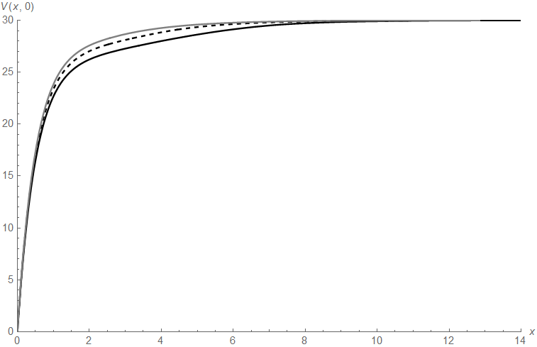
Figure 9.1: $V_{0}^{3}(x,0)$ (gray solid), $V_{0.5}^{3}(x,0)$ (dashed) and $V_{1}^{3}(x,0)$ (black solid) as a function of $x$.

Figure 9.2: $V_{0}^{3}(x)-V_{a}^{3}(x,0)$ for $a=0.2$ (dotted), $a=0.5$ (dashed), $a=0.8$ (dot-dashed) and $a=1$ (solid).

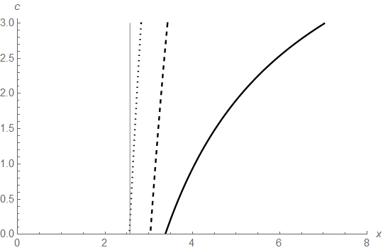
(a) $a=0.2$

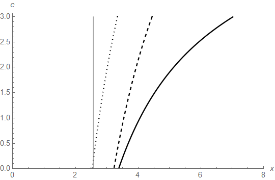
(b) $a=0.5$

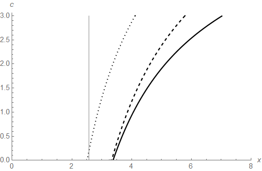
(c) $a=0.8$

Figure 9.3: Optimal drawdown curves $(\overline{\gamma}(c),c)$ (dotted) and $(\overline{\zeta}(c),c)\$(dashed) for $a=0.2,0.5,0.8$, together with the optimal threshold of the unconstrained problem ($a=0$, solid gray) and the optimal ratcheting curve $\left(\overline{\xi}(c),c\right)$ ($a=1$, solid black).

In order to see the impact of the drawdown restriction more clearly, in Figure 9.2 we plot the difference between $V_{0}^{\overline{c}}(x)$ (the unconstrained value function) and $V_{a}^{\overline{c}}(x,0)$ as a function of $x$ for increasingly restrictive drawdown levels $a=0.2$ (dotted), $a=0.5$ (dashed), $a=0.8$ (dot-dashed) and finally $a=1$ (ratcheting, solid). One observes that in particular for smaller values of $x$, the relaxation of ratcheting towards the drawdown constraint improves the performance of the resulting strategy quite a bit, although the relative gap between the performance of the ratcheting and the unconstrained case is anyway not so big (cf. Figure 9.1). The latter speaks in favor of the consideration of such strategies, as ratcheting and drawdown may be important for shareholders from a psychological point of view, and the efficiency loss when introducing these constraints is quite minor. In particular, if for a given initial surplus level $x$ one has a target efficiency loss one is willing to accept, results like Figure 9.2 can help to identify the corresponding drawdown coefficient $a$ that can still guarantee such a performance.

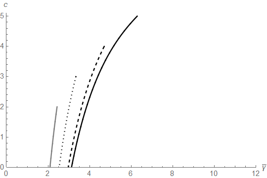
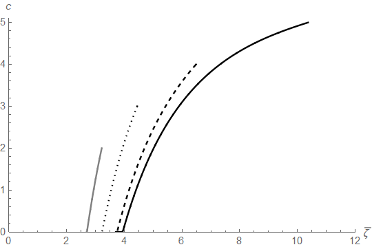
Figure 9.4: The curves $\overline{\gamma}^{\overline{c}}(c)$ (left) and $\overline{\zeta}^{\overline{c}}(c)$ (right) for $a=0.5$: $\overline{c}=2$ (solid gray), $\overline{c}=3$ (dotted), $\overline{c}=4=\mu$ (dashed) and $\overline{c}=5$ (solid black).

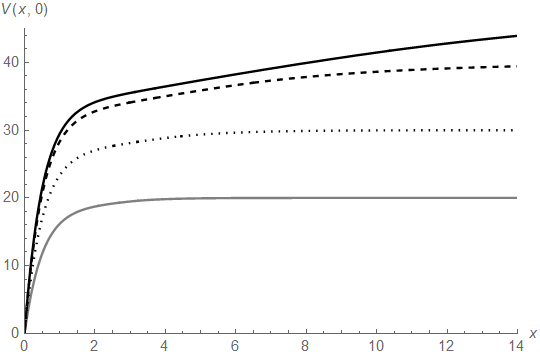
Figure 9.5: $V_{0.5}^{2}(x,0)$ (solid gray), $V_{0.5}^{3}(x,0)$ (dotted), $V_{0.5}^{4}(x,0)$ (dashed) and $V_{0.5}^{5}(x,0)$ (black solid) as a function of $x$.

In terms of the nature of the optimal strategy (which indeed turns out to be of two-curve type), Figures 9.3(a), 9.3(b) and 9.3(c) show the optimal drawdown curves $(\overline{\gamma}(c),c)$ (dotted) and $(\overline{\zeta}(c),c)\$(dashed) for $a=0.2$, $a=0.5$ and $a=0.8$, respectively. In all the plots we also depict the optimal threshold of the unconstrained dividend problem $a=0$ (solid gray) and the optimal ratcheting curve $\left(\overline{\xi}(c),c\right)$ for $a=1$ (solid black). To that end, recall from Asmussen and Taksar [7] that the optimal threshold for $a=0$ is given by

$$\frac{1}{\theta_{1}(0)-\theta_{2}(0)}\log\left(\frac{\theta_{2}(0)\;(\theta_{2}(0)-\theta_{2}(\overline{c}))}{\theta_{1}(0)\;(\theta_{1}(0)-\theta_{2}(\overline{c}))}\right)\text{,}$$

whereas the optimal strategy in the ratcheting case is given by a one-curve strategy which is obtained numerically according to the results in [1]. One can nicely see how the two curves $(\overline{\gamma}(c),c)$ and $(\overline{\zeta}(c),c)$ move towards the right as $a$ increases, interpolating between the unconstrained and the ratcheting case. Note that the resulting two-curve shapes are somewhat reminiscent of some figures obtained in Guo and Tomecek [22] for other types of singular control problems, where also a smooth-fit principle was established.

Also notice that the location of these curves can vary considerably as the maximally allowed dividend rate $\overline{c}$ changes. Figure 9.4 depicts $\overline{\gamma}^{\overline{c}}(c)$ and $\overline{\zeta}^{\overline{c}}(c)$ for $a=0.5$ for $\overline{c}$ growing from 2 to 5. In particular, when $\overline{c}$ is larger, the necessary surplus level $x$ to switch to higher dividend rates is larger as well. Figure 9.5 shows the corresponding value functions for these increasing values of $\overline{c}$ ($a=0.5$). Recall that while the drawdown constraint is not a major efficiency loss when compared to the unconstrained case for the same $\overline{c}$ (cf. Figure 9.1 for the case $\overline{c}=3$), the size of $\overline{c}$ itself naturally has a considerable impact on the size of the value function.

9.2 Boundary Conditions

Let us now investigate the situation when the maximally allowed dividend rate $\overline{c}$ becomes large. In addition to $a=0.5$ and $a=0.8$, we now also consider a smaller drawdown level $a=0.07$ (in order to illustrate the different monotonicity for small values of $a$, cf. Remark 7.2). One finds numerically that there exists a unique zero $z^{\ast}(\overline{c})$ of $C_{0}(b^{\ast}(\overline{c}),\cdot,\overline{c})$ in $(b^{\ast}(\overline{c}),\infty)$ for any $\overline{c}\geq 0$. We also have found that there exists a unique zero $x^{\ast}(\overline{c})$ in $(0,\infty)$ of $\partial_{\overline{c}}V^{\overline{c}}(\cdot,\overline{c})$ for $\overline{c}\geq 5.17$ for $a=0.07$; for $\overline{c}\geq 3.45$ for $a=0.5$ and for $\overline{c}\geq 2.52$ for $a=0.8$. Recall that we have proved in Propositions 7.1, 7.2 and 7.3 that $\lim_{\overline{c}\rightarrow\infty}b^{\ast}(\overline{c})=\mu/q$ and $\lim_{\overline{c}\rightarrow\infty}z^{\ast}(\overline{c})=\lim_{\overline{c}\rightarrow\infty}x^{\ast}(\overline{c})=\mu(1+1/\sqrt{a})/q$.
Figure 9.6 shows the curves of the boundary conditions $(b^{\ast}(\overline{c}),\overline{c})$, $(z^{\ast}(\overline{c}),\overline{c})$ and $(x^{\ast}(\overline{c}),\overline{c})$ for $a=0.07$, $a=0.5$ and $a=0.8$ respectively. In the case $a=0.07$ one sees how the limit $\mu(1+1/\sqrt{a})/q=191.2$ (vertical dotted line) is indeed approached from the right as $\overline{c}\rightarrow\infty$, whereas for $a=0.5$ and $a=0.8$ the respective limits $96.57$ and $84.72$ (vertical dotted line) are approached from the left, cf. Remark 7.2. It is important to keep in mind that these plots only depict the boundary value for each choice of $\overline{c}$, and are not to be confused with the optimal drawdown curves in Figure 9.3. Note that $x^{\ast}(\overline{c})$ and $z^{\ast}(\overline{c})$ are – already for moderate values of $\overline{c}$ – almost identical, with $z^{\ast}(\overline{c})>x^{\ast}(\overline{c})$, see Figure 9.7 for a graph of the difference $z^{\ast}(\overline{c})-$ $x^{\ast}(\overline{c})$ for $a=0.07$, $a=0.5$ and $a=0.8$ respectively. From the latter, one nicely sees $z^{\ast}(\overline{c})>x^{\ast}(\overline{c})$ (cf. Remark 7.1) as well as the asymptotic equivalence (7.10) of the two quantities.

In Figure 9.3 we saw that the curve $\overline{\zeta}^{\overline{c}}(c)$ is to the left of the ratcheting curve $\overline{\xi}^{\overline{c}}(c)$. At the same time for large values of $\overline{c}$, we know that $\overline{\zeta}^{\overline{c}}(c)$ must be to the right of $\overline{\xi}^{\overline{c}}(c)$, as

$$\lim_{\overline{c}\longrightarrow\infty}\overline{\xi}^{\overline{c}}(\overline{c})=\frac{2\mu}{q}<\frac{\mu}{q}\left(1+\frac{1}{\sqrt{a}}\right)=\lim_{\overline{c}\longrightarrow\infty}z^{\ast}(\overline{c})\text{.}$$

It is therefore of interest to see when this crossing for the limiting value takes place. Figure 9.8 depicts $z^{\ast}(\overline{c})$ (solid) and $\overline{\xi}^{\overline{c}}(\overline{c})$ (dotted) for $a=0.07$, $a=0.5$ and $a=0.8$ respectively. We see that indeed for $\overline{c}$ small, $z^{\ast}(\overline{c})<\overline{\xi}^{\overline{c}}(\overline{c})$ and for $\overline{c}$ large, $z^{\ast}(\overline{c})>\overline{\xi}^{\overline{c}}(\overline{c})$. Moreover, we obtain numerically that the intersection point of the curves of $z^{\ast}(\overline{c})\$and $\overline{\xi}^{\overline{c}}(\overline{c})$ occurs at $\overline{c}=39.70$ for $a=0.07$, at $\overline{c}=9.74$ for $a=0.5$, and at $\overline{c}=8.37$ for $a=0.8$ for the given set of parameters. That is, on from these values of $\overline{c}$, the possibility of the drawdown increases the value of surplus on from which one starts to pay the maximal dividend rate, when compared to pure ratcheting, and it is intuitive that the difference is less pronounced as $a$ increases.

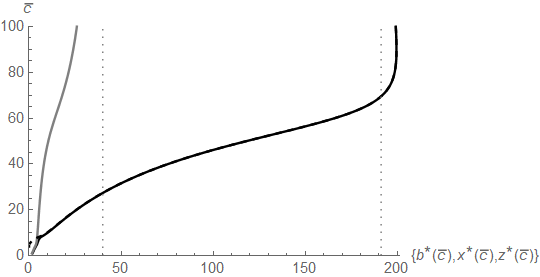
(a) $a=0.07$

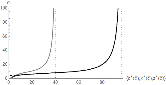
(b) $a=0.5$

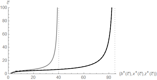
(c) $a=0.8$

Figure 9.6: The boundary condition values $b^{\ast}(\overline{c})$ (grey), $z^{\ast}(\overline{c})$ (solid) and $x^{\ast}(\overline{c})$ (dashed) as a function of $\overline{c}$ for different values of $a$.

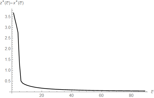
(a) $a=0.07$

(b) $a=0.5$

(c) $a=0.8$

Figure 9.7: The difference $z^{\ast}(\overline{c})-$ $x^{\ast}(\overline{c})$ as a function of $\overline{c}$ for different values of $a$.

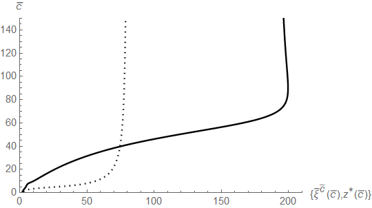
(a) $a=0.07$

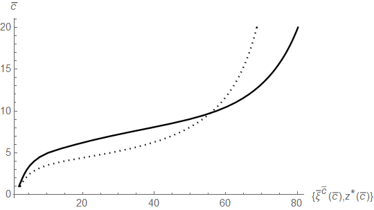
(b) $a=0.5$

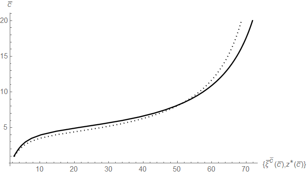
(c) $a=0.8$

Figure 9.8: The boundary values $z^{\ast}(\overline{c})\$ (solid) and the optimal ratcheting boundary value $\overline{\xi}^{\overline{c}}(\overline{c})$ (dotted) as $\overline{c}$ grows, for different values of $a$.

10 Conclusions

In this paper we addressed the problem of optimal dividends under a drawdown constraint. We showed that the value function can be expressed as the unique viscosity solution of a respective two-dimensional Hamilton-Jacobi-Bellman equation and derived conditions under which the optimal strategy is of a two-curve form. We conjecture that these conditions are in fact always fulfilled and – using a smooth-fit principle – could prove it for large values of current and maximal dividend rate $c$ and $\overline{c}$, respectively. For concrete numerical examples, we also proved the optimality of two-curve strategies numerically for small values of $c$ and $\overline{c}$, and showed how to identify the resulting optimal curves, which turns out to be a very challenging and technical task, involving the numerical solution of a highly involved system of ordinary differential equations and its boundary conditions. We illustrate how this can be concretely implemented for a moderate size of $\overline{c}$ ; for high values of $\overline{c}$ this is difficult numerically because the formulas involve algebraic sums with terms with exponentials with very large exponents and the computations require very high numerical precision. We furthermore showed that, when $\overline{c}$ tends to infinity, the curves converge to a finite limit, the size of which follows a surprisingly simple and intriguing formula in terms of the square-root of the drawdown percentage $a$, and irrespective of the size of the volatility parameter $\sigma$. The latter fact also allowed to get some intuition on the nature of this limit from the deterministic limit case $\sigma=0$.
Altogether, this paper for the first time explicitly addressed a drawdown constraint for a control problem in this context, and it turned out that the resulting strategies smoothly interpolate between the unconstrained problem and the situation with ratcheting constraints, allowing to get some quantitative insight in the efficiency gain when relaxing the ratcheting. It will be interesting to see whether other dividend – and more generally control – problems can be extended in a similar way. In particular, extending the results of the paper from the Brownian risk model to a compound Poisson surplus process may be an interesting endeavour, which would lead to a relaxation of the ratcheting problem studied in [2]. Another future direction of research may be to extend the approach of this paper to incorporate constraints on the dividend rate in terms of an average of its previous values, for instance along the lines of Angoshtari et al. [6].

11 Appendix: Some Formulas

In the following, we state some definitions and formulas referred to earlier in the paper in a compact way.

$$d(y,z,c) =e^{y\theta_{2}(ac)+(z-y)\theta_{1}(c)}\theta_{2}(c)-e^{(z-y)\theta_{1}(c)+y\theta_{1}(ac)}\theta_{2}(c)+e^{(z-y)\theta_{2}(c)+y\theta_{2}(ac)}\theta_{2}(ac)$$

$$-e^{y\theta_{2}(ac)+(z-y)\theta_{1}(c)}\theta_{2}(ac)+e^{(z-y)\theta_{2}(c)}\left(-e^{y\theta_{2}(ac)}+e^{y\theta_{1}(ac)}\right)\theta_{1}(c)$$

$$+e^{y\theta_{1}(ac)}\left(-e^{(z-y)\theta_{2}(c)}+e^{(z-y)\theta_{1}(c)}\right)\theta_{1}(ac),$$

$$b_{00}(y,z,c) =ae^{(z-y)\theta_{2}(c)+y\theta_{2}(ac)}\theta_{2}(ac)\left(\theta_{2}(c)-\theta_{1}(c)\right)-e^{(z-y)\theta_{1}(c)}\theta_{2}(c)\left(\theta_{1}(c)-\theta_{2}(c)\right)$$

$$-ae^{(z-y)\theta_{1}(c)}\left(-1+e^{y\theta_{2}(ac)}\right)\theta_{2}(c)\left(\theta_{1}(c)-\theta_{2}(c)\right)$$

$$+ae^{y\theta_{2}(ac)+(z-y)\theta_{1}(c)}\theta_{2}(ac)\left(\theta_{1}(c)-\theta_{2}(c)\right)+e^{(z-y)\theta_{2}(c)}\theta_{1}(c)\left(\theta_{1}(c)-\theta_{2}(c)\right)$$

$$+ae^{(z-y)\theta_{2}(c)}\left(-1+e^{y\theta_{2}(ac)}\right)\theta_{1}(c)\left(\theta_{1}(c)-\theta_{2}(c)\right)$$

$$-\left(\theta_{1}(c)-\theta_{2}(c)\right){}^{2}-e^{(z-y)\theta_{1}(c)}\left(c+ac\left(-1+e^{y\theta_{2}(ac)}\right)\right)\left(\theta_{1}(c)-\theta_{2}(c)\right)\theta_{2}^{\prime}(c)$$

$$+e^{(z-y)\theta_{2}(c)}(z-y)\left(\theta_{1}(c)-\theta_{2}(c)\right)\left(-ace^{y\theta_{2}(ac)}\theta_{2}(ac)+c\left(1+a\left(-1+e^{y\theta_{2}(ac)}\right)\right)\theta_{1}(c)\right)\theta_{2}^{\prime}(c)$$

$$+a^{2}ce^{(z-y)\theta_{2}(c)+y\theta_{2}(ac)}\left(\theta_{2}(c)-\theta_{1}(c)\right)\theta_{2}^{\prime}(ac)+a^{2}ce^{(z-y)\theta_{2}(c)+y\theta_{2}(ac)}y\theta_{2}(ac)\left(\theta_{2}(c)-\theta_{1}(c)\right)\theta_{2}^{\prime}(ac)$$

$$+a^{2}ce^{y\theta_{2}(ac)+(z-y)\theta_{1}(c)}\left(\theta_{1}(c)-\theta_{2}(c)\right)\theta_{2}^{\prime}(ac)-a^{2}ce^{y\theta_{2}(ac)+(z-y)\theta_{1}(c)}y\theta_{2}(c)\left(\theta_{1}(c)-\theta_{2}(c)\right)\theta_{2}^{\prime}(ac)$$

$$+a^{2}ce^{y\theta_{2}(ac)+(z-y)\theta_{1}(c)}y\theta_{2}(ac)\left(\theta_{1}(c)-\theta_{2}(c)\right)\theta_{2}^{\prime}(ac)+a^{2}ce^{(z-y)\theta_{2}(c)+y\theta_{2}(ac)}y\theta_{1}(c)\left(\theta_{1}(c)-\theta_{2}(c)\right)\theta_{2}^{\prime}(ac)$$

$$+e^{(z-y)\theta_{2}(c)}\left(c+ac\left(-1+e^{y\theta_{2}(ac)}\right)\right)\left(\theta_{1}(c)-\theta_{2}(c)\right)\theta_{1}^{\prime}(c)$$

$$+ce^{(z-y)\theta_{1}(c)}(y-z)\left(\theta_{2}(c)+a\left(-1+e^{y\theta_{2}(ac)}\right)\theta_{2}(c)-ae^{y\theta_{2}(ac)}\theta_{2}(ac)\right)\left(\theta_{1}(c)-\theta_{2}(c)\right)\theta_{1}^{\prime}(c)$$

$$+e^{(z-y)\theta_{1}(c)}\left(c\left(1+a\left(-1+e^{y\theta_{2}(ac)}\right)\right)\theta_{2}(c)-ace^{y\theta_{2}(ac)}\theta_{2}(ac)\right)\left(-\theta_{2}^{\prime}(c)+\theta_{1}^{\prime}(c)\right)$$

$$+ce^{(z-y)\theta_{2}(c)}\left(ae^{y\theta_{2}(ac)}\theta_{2}(ac)+\left(-1+a-ae^{y\theta_{2}(ac)}\right)\theta_{1}(c)\right)\left(-\theta_{2}^{\prime}(c)+\theta_{1}^{\prime}(c)\right),$$

$$b_{01}(y,z,c) =c\left(\theta_{1}(c)-\theta_{2}(c)\right)$$

$$\left(ae^{y\theta_{2}(ac)}\theta_{2}(ac)\left(-\theta_{2}(c)+\theta_{2}(ac)\right)+\left(\theta_{2}(c)+a\left(-1+e^{y\theta_{2}(ac)}\right)\theta_{2}(c)-ae^{y\theta_{2}(ac)}\theta_{2}(ac)\right)\theta_{1}(c)\right),$$

$$b_{10}(y,z,c) =e^{(-y+z)\theta_{2}(c]}\left(e^{y\theta_{1}(ac)}-e^{y\theta_{2}(ac)}\right)\left(-\theta_{1}(c)+\theta_{2}(c)\right)\theta_{1}^{\prime}(c)$$

$$-e^{(-y+z)\theta_{1}(c)}(y-z)\left(\theta_{1}(c)-\theta_{2}(c)\right)\left(-e^{y\theta_{1}(ac)}\theta_{1}(ac)+\left(e^{y\theta_{1}(ac)}-e^{y\theta_{2}(ac)}\right)\theta_{2}(c)+e^{y\theta_{2}(ac)}\theta_{2}(ac)\right)\theta_{1}^{\prime}(c)$$

$$-ae^{(-y+z)\theta_{1}(c)+y\theta_{1}(ac)}\left(\theta_{1}(c)-\theta_{2}(c)\right)\theta_{1}^{\prime}(ac)+ae^{y\theta_{1}(ac)+(-y+z)\theta_{2}(c)}\left(\theta_{1}(c)-\theta_{2}(c)\right)\theta_{1}^{\prime}(ac)$$

$$-ae^{(-y+z)\theta_{1}(c)+y\theta_{1}(ac)}y\theta_{1}(ac)\left(\theta_{1}(c)-\theta_{2}(c)\right)\theta_{1}^{\prime}(ac)$$

$$+ae^{y\theta_{1}(ac)+(-y+z)\theta_{2}(c)}y\theta_{1}(ac)\left(\theta_{1}(c)-\theta_{2}(c)\right)\theta_{1}^{\prime}(ac)$$

$$-e^{(-y+z)\theta_{2}(c)}\left(\left(-e^{y\theta_{1}(ac)}+e^{y\theta_{2}(ac)}\right)\theta_{1}(c)+e^{y\theta_{1}(ac)}\theta_{1}(ac)-e^{y\theta_{2}(ac)}\theta_{2}(ac)\right)\left(\theta_{1}^{\prime}(c)-\theta_{2}^{\prime}(c)\right)$$

$$+e^{(-y+z)\theta_{1}(c)}\left(e^{y\theta_{1}(ac)}\theta_{1}(ac)+\left(-e^{y\theta_{1}(ac)}+e^{y\theta_{2}(ac)}\right)\theta_{2}(c)-e^{y\theta_{2}(ac)}\theta_{2}(ac)\right)\left(\theta_{1}^{\prime}(c)-\theta_{2}^{\prime}(c)\right)$$

$$+e^{(-y+z)\theta_{1}(c)}\left(e^{y\theta_{1}(ac)}-e^{y\theta_{2}(ac)}\right)\left(\theta_{1}(c)-\theta_{2}(c)\right)\theta_{2}^{\prime}(c)$$

$$+e^{(-y+z)\theta_{2}(c)}(-y+z)\left(\theta_{1}(c)-\theta_{2}(c)\right)\left(\left(-e^{y\theta_{1}(ac)}+e^{y\theta_{2}(ac)}\right)\theta_{1}(c)+e^{y\theta_{1}(ac)}\theta_{1}(ac)-e^{y\theta_{2}(ac)}\theta_{2}(ac)\right)\theta_{2}^{\prime}(c)$$

$$+ae^{(-y+z)\theta_{1}(c)+y\theta_{2}(ac)}\left(\theta_{1}(c)-\theta_{2}(c)\right)\theta_{2}^{\prime}(ac)$$

$$+ae^{(-y+z)\theta_{2}(c)+y\theta_{2}(ac)}\left(-\theta_{1}(c)+\theta_{2}(c)\right)\theta_{2}^{\prime}(ac)+ae^{(-y+z)\theta_{1}(c)+y\theta_{2}(ac)}y\left(\theta_{1}(c)-\theta_{2}(c)\right)\theta_{2}(ac)\theta_{2}^{\prime}(ac)$$

$$+ae^{(-y+z)\theta_{2}(c)+y\theta_{2}(ac)}y\left(-\theta_{1}(c)+\theta_{2}(c)\right)\theta_{2}(ac)\theta_{2}^{\prime}(ac)$$

$$-ae^{(-y+z)\theta_{2}(c)}y\theta_{1}(c)\left(\theta_{1}(c)-\theta_{2}(c)\right)\left(e^{y\theta_{1}(ac)}\theta_{1}^{\prime}(ac)-e^{y\theta_{2}(ac)}\theta_{2}^{\prime}(ac)\right)$$

$$+ae^{(-y+z)\theta_{1}(c)}y\left(\theta_{1}(c)-\theta_{2}(c)\right)\theta_{2}(c)\left(e^{y\theta_{1}(ac)}\theta_{1}^{\prime}(ac)-e^{y\theta_{2}(ac)}\theta_{2}^{\prime}(ac)\right)$$

and

$$b_{11}(y,z,c) =-(\text{$\theta_{1}(c)$}-\text{$\theta_{2}(c)$})$$

$$\left(e^{y\text{$\theta_{1}(ac)$}}(\theta_{1}(ac)-\theta_{1}(c))(\theta_{1}(ac)-\theta_{2}(c))+e^{y\text{$\theta_{2}(ac)$}}(\theta_{2}(c)-\theta_{2}(ac))(\theta_{2}(ac)-\theta_{1}(c))\right)$$

$$f_{10}(x,c)=\frac{ca}{q}(1-e^{\theta_{2}(ac)x}),$$

$$f_{11}(x,c)=e^{\theta_{1}(ac)x}-e^{\theta_{2}(ac)x},$$

$$f_{20}(y,x,c) =\frac{c}{q(\text{$\theta_{2}(c)$}-\text{$\theta_{1}(c)$})}$$

$$(\text{$\theta_{2}(c)+(a-1)$}e^{\theta_{1}(c)(x-y)}\text{$\theta_{2}(c)+a$}e^{y\theta_{2}(ac)}(-e^{\theta_{2}(c)(x-y)}\theta_{2}(ac)+e^{\theta_{1}(c)(x-y)}(\theta_{2}(ac)-\theta_{2}(c)))$$

$$+\theta_{1}(c)(-1+e^{\theta_{2}(c)(x-y)}(1+a(e^{y\theta_{2}(ac)}-1)))),$$

$$f_{21}(y,x,c) =\frac{1}{\text{$\theta_{1}(c)$}-\text{$\theta_{2}(c)$}}$$

$$(e^{y\text{$\theta_{2}(ac)$}}(e^{\theta_{1}(c)(x-y)}(\text{$\theta_{2}(c)-\theta_{2}(ac))+$}e^{\theta_{2}(c)(x-y)}(\theta_{2}(ac)-\text{$\theta_{1}(c)$}))$$

$$+e^{y\text{$\theta_{1}(ac)$}}(e^{\theta_{2}(c)(x-y)}(\text{$\theta_{1}(c)-\theta_{1}(ac))+$}e^{\theta_{1}(c)(x-y)}(\theta_{1}(ac)-\text{$\theta_{2}(c)$}))$$

$$=\frac{d(y,x,c)}{\text{$\theta_{1}(c)$}-\text{$\theta_{2}(c)$}}$$

$$C_{0}(y,z,c)=b_{11}(y,c)\partial_{z}\left(\frac{b_{00}(y,z,c)}{d(y,z,c)}\right)-b_{01}(y,c)\partial_{z}\left(\frac{b_{10}(y,z,c)}{d(y,z,c)}\right)$$

$$C_{11}(y,z,c)=b_{11}(y,c)\partial_{y}\left(\frac{(e^{(z-y)\theta_{1}(c)}-e^{(z-y)\theta_{2}(c)})b_{01}(y,c)}{d(y,z,c)}\right)-~{}b_{01}(y,c)\partial_{y}\left(\frac{(e^{(z-y)\theta_{1}(c)}-e^{(z-y)\theta_{2}(c)})b_{11}(y,c)}{d(y,z,c)}\right)$$

$$C_{10}(y,z,c)=b_{01}(y,c)\partial_{y}\left(\frac{b_{10}(y,z,c)}{d(y,z,c)}\right)-b_{11}(y,c)\partial_{y}\left(\frac{b_{00}(y,z,c)}{d(y,z,c)}\right)$$

$$C_{21}(y,z,c)=\partial_{y}C_{0}(y,z,c)=\partial_{y}\left(b_{11}(y,c)\partial_{z}\left(\frac{b_{00}(y,z,c)}{d(y,z,c)}\right)-b_{01}(y,c)\partial_{z}\left(\frac{b_{10}(y,z,c)}{d(y,z,c)}\right)\right)$$

$$C_{22}(y,z,c)=\partial_{z}C_{0}(y,z,c)=\partial_{z}\left(b_{11}(y,c)\partial_{z}\left(\frac{b_{00}(y,z,c)}{d(y,z,c)}\right)-b_{01}(y,c)\partial_{z}\left(\frac{b_{10}(y,z,c)}{d(y,z,c)}\right)\right)$$

$$C_{20}(y,z,c)=-\partial_{c}C_{0}(y,z,c)=-\partial_{c}\left(b_{11}(y,c)\partial_{z}\left(\frac{b_{00}(y,z,c)}{d(y,z,c)}\right)-b_{01}(y,c)\partial_{z}\left(\frac{b_{10}(y,z,c)}{d(y,z,c)}\right)\right)$$

$$\left(\begin{array}[c]{c}g_{{}_{1}}(y,z,c)\\ g_{2}(y,z,c)\\ g_{3}(y,z,c)\\ g_{4}(y,z,c)\\ g_{{}_{5}}(y,z,c)\\ g_{{}_{6}}(y,z,c)\\ g_{{}_{7}}(y,z,c)\\ g_{{}_{8}}(y,z,c)\\ g_{{}_{9}}(y,z,c)\\ g_{{}_{10}}(y,z,c)\\ g_{{}_{11}}(y,z,c)\\ g_{{}_{12}}(y,z,c)\\ g_{{}_{13}}(y,z,c)\\ g_{{}_{14}}(y,z,c)\\ g_{{}_{15}}(y,z,c)\\ g_{{}_{16}}(y,z,c)\end{array}\right)=\left(\begin{array}[c]{cccc}0&1&0&2\\ 0&2&0&2\\ 1&0&0&2\\ 1&1&0&2\\ 0&2&1&2\\ 1&0&1&1\\ 1&1&1&1\\ 1&1&1&2\\ 0&1&2&0\\ 0&2&2&0\\ 0&2&2&1\\ 1&0&2&0\\ 1&1&2&0\\ 1&1&2&1\\ 0&2&1&1\\ 0&1&1&1\end{array}\right)\cdot\left(\begin{array}[c]{c}(z-y)\theta_{1}(c)\\ (z-y)\theta_{2}(c)\\ y\theta_{1}(ac)\\ y\theta_{2}(ac)\end{array}\right)$$

$$\left(\begin{array}[c]{c}h_{{}_{1}}(x,b,c)\\ h_{2}(x,b,c)\\ h_{3}(x,b,c)\\ h_{4}(x,b,c)\\ h_{{}_{5}}(x,b,c)\\ h_{{}_{6}}(x,b,c)\\ h_{{}_{7}}(x,b,c)\\ h_{{}_{8}}(x,b,c)\\ h_{{}_{9}}(x,b,c)\\ h_{{}_{10}}(x,b,c)\\ h_{{}_{11}}(x,b,c)\end{array}\right)=\left(\begin{array}[c]{cccc}2&0&0&0\\ 1&1&0&0\\ 0&0&2&0\\ 0&0&1&1\\ 1&0&1&0\\ 0&1&1&0\\ 1&1&1&0\\ 0&1&2&0\\ 1&0&0&1\\ 2&0&0&1\\ 1&0&1&1\end{array}\right)\cdot\left(\begin{array}[c]{c}b\theta_{1}(ac)\\ x\theta_{1}(ac)\\ b\theta_{2}(ac))\\ x\theta_{2}(ac)\end{array}\right)$$

$$\left(\begin{array}[c]{c}k_{{}_{1}}(x,b,c)\\ k_{2}(x,b,c)\\ k_{3}(x,b,c)\\ k_{4}(x,b,c)\\ k_{{}_{5}}(x,b,c)\\ k_{{}_{6}}(x,b,c)\\ k_{{}_{7}}(x,b,c)\\ k_{{}_{8}}(x,b,c)\end{array}\right)=\left(\begin{array}[c]{ccc}2&0&0\\ 2&0&1\\ 0&2&0\\ 1&1&0\\ 1&1&1\\ 2&1&1\\ 0&2&1\\ 1&2&1\end{array}\right)\cdot\left(\begin{array}[c]{c}b\theta_{1}(ac)\\ b\theta_{2}(ac)\\ (x-b)\theta_{2}(c))\end{array}\right).$$

References

[1]Albrecher, H., Azcue, P. and Muler N. (2022). Optimal
ratcheting of dividends in a Brownian model. SIAM J. Financial Math.,
to appear.
[2]Albrecher, H., Azcue, P. and Muler N. (2020), Optimal ratcheting
of dividends in insurance. SIAM Journal on Control and Optimization,
58(4), 1822–1845.
[3]Albrecher H., Bäuerle N. and Bladt M. (2018). Dividends:
From refracting to ratcheting. Insurance Math. Econom.83, 47–58.
[4]Albrecher, H. and Thonhauser, S. (2009). Optimality results for
dividend problems in insurance. RACSAM-Revista de la Real Academia de
Ciencias Exactas, Fisicas y Naturales. Serie A. Matematicas103,
No.2, 295–320.
[5]Angoshtari, B., Bayraktar, E. and Young, V.R. (2019) Optimal
dividend distribution under drawdown and ratcheting constraints on dividend
rates. SIAM Journal on Financial Mathematics10, 2, 547–577.
[6]Angoshtari, B., Bayraktar, E. and Young, V.R. (2020) Optimal
Consumption under a Habit-Formation Constraint. SIAM Journal on
Financial Mathematics13, 1, 321–352.
[7]Asmussen, S.and Taksar, M. (1997). Controlled diffusion
models for optimal dividend pay-out. Insurance: Mathematics and
Economics20, 1, 1-15.
[8]Avanzi, B. (2009). Strategies for dividend distribution: A
review. North American Actuarial Journal13, 2, 217-251.
[9]Azcue P. and Muler N. (2014). Stochastic
Optimization in Insurance: a Dynamic Programming Approach. Springer Briefs in
Quantitative Finance. Springer.
[10]Borodin, A. N. and Salminen, P. (2002).
Handbook of Brownian Motion—Facts and Formulae. 2nd ed.
Birkhäuser, Basel.
[11]Brinker, L.V. (2021). Stochastic Optimisation of
Drawdowns via Dynamic Reinsurance Controls. Doctoral Dissertation,
Universität zu Köln.
[12]Brinker, L.V. and Schmidli, H. (2022) Optimal discounted
drawdowns in a diffusion approximation under proportional reinsurance.
Journal of Applied Probability, to appear.
[13]Claisse, J., Talay, D. and Tan, X. (2016). A pseudo-Markov
property for controlled diffusion processes. SIAM Journal on Control
and Optimization, 54, 2, 1017-1029.
[14]Chen, X., Landriault, D., Li, B. and Li, D. (2015). On
minimizing drawdown risks of lifetime investments. Insurance:
Mathematics and Economics65, 46–54.
[15]De Finetti, B. (1957). Su un’Impostazione Alternativa della
Teoria Collettiva del Rischio. Transactions of the 15th Int. Congress
of Actuaries2, 433–443.
[16]Dybvig, P.H. (1995). Dusenberry’s ratcheting of consumption:
optimal dynamic consumption and investment given intolerance for any decline
in standard of living.The Review of Economic Studies62, 2, 287–313.
[17]Eisenberg, J., Grandits, P. and Thonhauser, S. (2014). Optimal
consumption under deterministic income. Journal of Optimization Theory
and Applications160,1, 255-279.
[18]Elie, R. and Touzi, N. (2008). Optimal lifetime consumption and
investment under a drawdown constraint. Finance and Stochastics12, 3, 299–330.
[20]Gerber, H. U. (1972). Games of economic survival with
discrete-and continuous-income processes. Operations Research 20, 1, 37–45.
[21]Gerber, H. U. and Shiu, E.S.W. (2004). Optimal dividends:
analysis with Brownian motion. North American Actuarial Journal,
8, 1, 1–20.
[22]Guo, X. and Tomecek, P. (2009). A class of singular control
problems and the smooth fit principle. SIAM Journal on Control and
Optimization47, 6, 3076-3099.
[23]Jeanblanc-Picqué, M. and Shiryaev, A. (1995)
Optimization of the flow of dividends. Uspekhi Mat. Nauk50,
2(302), 25–46.
[24]Kardaras, C., Obloj, J. and Platen, E. (2017). The numéraire
property and long-term growth optimality for drawdown-constrained investments.
Mathematical Finance27, 1, 68–95.
[25]Landriault, D., Li, B. and Zhang, H. (2017). On magnitude,
asymptotics and duration of drawdowns for Lévy models. Bernoulli23, 1, 432–458.
[26]Loeffen, R.L. and Renaud, J. F. (2010). De Finetti’s
optimal dividends problem with an affine penalty function at ruin.
Insurance: Mathematics and Economics46,1, 98-108.
[27]Radner, R. Shepp, L. (1996) Risk vs.profit potential: a model
for corporate strategy. J. Econom. Dynamics Control20, 1373–1393.
[28]Schmidli, H. (2008). Stochastic Control
in Insurance. Springer, New York.
[29]Shreve, S.E., Lehoczky J.P. and Gaver, D.P. (1984) Optimal
consumption for general diffusions with absorbing and reflecting
barriers. SIAM J. Control Optim.22, 1, 55–75.