Gravitational Form Factors and Mechanical Properties of the Proton : Connection Between Distributions in 2D and 3D

Abstract

The gravitational form factors which are obtained from the matrix elements of the energy momentum tensor provide us information about internal distributions of mass, energy, pressure and shear. The Druck term is the least understood among all the gravitational form factor. In a light front quark-diquark model of proton, we investigate the Druck form factor. Using Abel transformation, we evaluate the 3D distribution in the Breit frame from the 2D light front distributions. The results are compared with other models and lattice predictions.

I INTRODUCTION

Form factors are sources of information about the internal structure of hadron. There are several form factors that give a different kind of information about the hadron. Hadron structures are probed by electromagnetic, weak, and gravitational interactions where particles couple to the matter fields. In electromagnetic interaction photon couples to matter field and the corresponding conserved electromagnetic current gives electric and magnetic charge distributions inside the hadron through form factors. The weak interaction which is mediated through $W_{\pm}$ and $Z$ bosons provide axial and pseudoscalar form factors of the proton. The gravitational interaction between graviton-proton provides mass, spin, and force distribution inside the proton Polyakov:2018zvc ; Lorce:2018egm . Corresponding form factors are known as gravitational form factors and are written as matrix elements of the energy-momentum tensor (EMT) Kobzarev:1962wt ; Pagels:1966zza . The electromagnetic and weak properties of the proton are well known but the internal mass or energy distributions, the forces on the quarks, and the angular momentum distribution inside the proton have attracted a lot of attention only recently.
In the forward limit, the electromagnetic form factors are equivalent to electric charge and magnetic moment and the weak interaction form factors are equivalent to the axial charge and pseudoscalar coupling while gravitational interaction describes mass, spin, and D-term Polyakov:1999gs ; Kivel:2000fg in this limit. The matrix element of EMT describes the response of the nucleon to a change in the external space-time metric. The components of the energy-momentum tensor tell us how matter couples to the gravitational field. The gravitational form factors are accessible through hard exclusive processes like deeply virtual Compton scattering as the second moments of Generalized Parton distribution functions (GPDs) Muller:1994ses ; Ji:1996ek ; Radyushkin:1996nd ; Radyushkin:1996ru . In Rajan:2018zzy a connection had been established between observables from high energy experiments and from the analysis of gravitational wave events. In the standard EMT parametrization, there are three gravitational form factors (GFFs). The GFFs $A(Q^{2})$, $J(Q^{2})$, and $D(Q^{2})$ correspond to the time-time, time-space, and space-space components of the energy-momentum tensor, respectively. At zero momentum transfer, $Q^{2}=0$ the GFFs $A(Q^{2})$ and $J(Q^{2})$ are constrained by proton mass and spin respectively. The D-term form factor is the new and most exciting one which is extracted through the spatial-spatial component of the energy-momentum tensor and encodes the information on shear forces and pressure distribution inside the proton Polyakov:2002yz . It has been calculated in several models and theories in the literature. In Polyakov:2002yz it was shown for the first time how GPDs can give information on the mechanical properties of the proton in a DVCS process, as they are extracted from the beam charge asymmetry in deeply virtual Compton scattering. While in Burkert:2018bqq ; Burkert:2021ith the JLab group reported the first determination of the pressure and shear forces on quarks inside the proton from experimental data on deeply virtual Compton scattering. The EMT form factors of the nucleon have been investigated in various approaches, for example, in lattice QCD Gockeler:2003jfa ; Hagler:2003jd ; Shanahan:2018nnv in chiral perturbation theory Dorati:2007bk ; Chen:2001pva ; Belitsky:2002jp ; Diehl , in the chiral quark-soliton model Goeke:2007fp ; Kim:2021jjf as well as in the Skyrme model Cebulla:2007ei ; Kim:2012ts .

The pressure, shear and energy distributions are usually defined in terms of the static EM tensor in the Breit frame. In relativistic field theory, one cannot localize a particle within a Compton wavelength, in other words, the three dimensional distributions defined in the Breit frame are subject to relativistic corrections. Alternatively, for a relativistic system, one can define them in the so-called infinite momentum frame, or light front quantization, where such relativistic effects are already incorporated. In Lorce:2018egm the mechanical properties like pressure, shear and energy distributions of a nucleon in two dimensions were introduced in the light front formalism, also later were discussed in Freese:2021czn . While in some models one can easily calculate the 3D distributions, in some cases, for example in light-front wavefunction approach it is easier to calculate the 2D distributions. In Panteleeva:2021iip it was shown that the 2D and 3D distributions can be connected through Abel transformation, which would make the intuitive understanding of these distributions more clear, particularly for relativistic systems like a nucleon. In a previous work, Chakrabarti:2020kdc the GFFs and the two-dimensional pressure, shear and energy distributions were investigated in the spectator type model motivated by ADs/QCD. In this work, we use the same model to obtain pressure, shear and energy distributions of the nucleon in 3D using invertible Abel transformation. The outline of the present work is as follows: in II we briefly review the light front formalism based on the light-front quark diquark model. In III we illustrate the definition of the gravitational form factors as matrix elements of the energy-momentum tensor and define the form factors in LFQDQ. Then in IV we focus on the extraction of $D(Q^{2})$ using two different approaches. And in V we show the 3D BF distributions which are the Abel image of the 2D light-front distributions by doing the inverse Abel transformation. And finally, in VI we present the summary and conclusion.

II LIGHT-FRONT QUARK-DIQUARK MODEL

In this model, the incoming photon, carrying a high momentum, interacts with one of the valence quarks inside the nucleon, and the other two valence quarks form a spectator diquark state of spin-0 (scalar diquark). Therefore the nucleon state $|P,S\rangle$ having momentum $P$ and spin $S$, can be represented as a two-particle Fock-state. In this article we consider the quark-scalar diquark model proposed inGutsche:2013zia . We use the light-cone convention $x^{\pm}=x^{0}\pm x^{3}$, and choose a frame where the transverse momentum of the proton vanishes, i.e. $P\equiv\left(P^{+},\frac{M^{2}}{P^{+}},\mathbf{0}_{\perp}\right)$, while the momentum of the quark and the diquark are $p\equiv\left(xP^{+},\frac{p^{2}+|\mathbf{p}_{\perp}^{2}|}{xP^{+}},\mathbf{p}_{\perp}\right)$ and $P_{X}\equiv\left((1-x)P^{+},P_{X}^{-},-\mathbf{p}_{\perp}\right)$ respectively, where $x=p^{+}/P^{+}$ is the longitudinal momentum fraction of the active quark. The two particle Fock-state expansion for the state with helicity $\pm\frac{1}{2}$ is given by

$$|P;\pm\rangle = \sum_{q}\int\frac{dxd^{2}\mathbf{p}_{\perp}}{2(2\pi)^{3}\sqrt{x(1-x)}}$$ (1)

$$\times\left[\psi_{+}^{q\pm}\left(x,\mathbf{p}_{\perp}\right)\left|+\frac{1}{2},0;xP^{+},\mathbf{p}_{\perp}\right\rangle+\psi_{-}^{q\pm}\left(x,\mathbf{p}_{\perp}\right)\left|-\frac{1}{2},0;xP^{+},\mathbf{p}_{\perp}\right\rangle\right],$$

where $|\lambda_{q},\lambda_{s};xP^{+},\mathbf{p}_{\perp}\rangle$ represents the two particle state with a quark having spin $\lambda_{q}=\pm\frac{1}{2}$, momentum $p$ and a scalar spectator diquark with spin $\lambda_{S}=0$. The two particle states are normalized as

$$\left\langle\lambda_{q}^{\prime},\lambda_{s}^{\prime};x^{\prime}P^{+},\mathbf{p}_{\perp}^{\prime}\mid\lambda_{q},\lambda_{s};xP^{+},\mathbf{p}_{\perp}\right\rangle=\prod_{i=1}^{2}16\pi^{3}p_{i}^{+}\delta\left(p_{i}^{\prime+}-p_{i}^{+}\right)\delta^{2}\left(\mathbf{p}_{\perp i}^{\prime}-\mathbf{p}_{\perp i}\right)\delta_{\lambda_{i}^{\prime}\lambda_{i}}.$$ (2)

Here $\psi_{\lambda_{q}}^{q\lambda_{N}}$ are the light-front wave functions with nucleon helicities $\lambda_{N}=\pm$. The LFWFs are given byGutsche:2013zia .

$$\psi_{+}^{q+}\left(x,\mathbf{p}_{\perp}\right) =\varphi^{q(1)}\left(x,\mathbf{p}_{\perp}\right)$$ (3)

$$\psi_{-}^{q+}\left(x,\mathbf{p}_{\perp}\right) =-\frac{p^{1}+ip^{2}}{xM}\varphi^{q(2)}\left(x,\mathbf{p}_{\perp}\right)$$

$$\psi_{+}^{q-}\left(x,\mathbf{p}_{\perp}\right) =\frac{p^{1}-ip^{2}}{xM}\varphi^{q(2)}\left(x,\mathbf{p}_{\perp}\right)$$

$$\psi_{-}^{q-}\left(x,\mathbf{p}_{\perp}\right) =\varphi^{q(1)}\left(x,\mathbf{p}_{\perp}\right)$$

where $\varphi_{q}^{(1)}(x,\mathbf{p}_{\perp})$ and $\varphi_{q}^{(2)}(x,\mathbf{p}_{\perp})$ are the wave functions predicted by the soft-wall AdS/QCD and can be written as

$$\varphi^{q(i)}\left(x,\mathbf{p}_{\perp}\right)=N_{q}^{(i)}\frac{4\pi}{\kappa}\sqrt{\frac{\log(1/x)}{1-x}}x^{a_{q}^{(i)}}(1-x)^{b_{q}^{(i)}}\exp\left[-\frac{\mathbf{p}_{\perp}^{2}}{2\kappa^{2}}\frac{\log(1/x)}{(1-x)^{2}}\right];$$ (4)

where $\kappa=0.4$ GeV is the AdS/QCD scale parameter and the quarks are assumed to be massless Brodsky:2006ha . The values of the model parameters $a_{q}^{i}$ and $b_{q}^{i}$ and the normalization constants $N_{q}^{i}$ at an initial scale $\mu_{0}^{2}=0.32$ GeV² were fixed by fitting the nucleon electromagnetic form factors and can be found in ref. Chakrabarti:2015ama . The wave functions can be reduced to the form predicted by AdS/QCD for $a_{q}^{i}=b_{q}^{i}=0$ deTeramond:2011aml .

III RELATIONS BETWEEN 2D LIGHT FRONT DISTRIBUTIONS AND 3D BREIT FRAME DISTRIBUTIONS

As discussed in the Introduction, in case of nucleons there are three independent EMT form factors Ji:1996ek ; Ji:2012vj ; Harindranath:2013goa ; Pagels:1966zza ; Kobzarev:1962wt

$$\left\langle p^{\prime}\left|\hat{\Theta}_{\mathrm{QCD}}^{\mu\nu}(0)\right|p\right\rangle= \bar{u}\left(p^{\prime}\right)\left[A(t)\frac{P^{\mu}P^{\nu}}{M}+J(t)\frac{iP^{\{\mu}\sigma^{\nu\}{\alpha}}\Delta_{\alpha}}{M}\right.$$ (5)

$$\left.+\frac{D(t)}{4M}\left(\Delta^{\mu}\Delta^{\nu}-\eta^{\mu\nu}\Delta^{2}\right)\right]u(p),$$

where $\hat{\Theta}_{\mathrm{QCD}}^{\mu\nu}(x)$ is the symmetric EMT operator of QCD. $P=(p+p^{\prime})/2,\Delta=p^{\prime}-p,t=\Delta^{2}$, and the symmetrization operator is defined as $X_{\{\mu}Y_{\nu\}}=\frac{1}{2}(X_{\mu}Y_{\nu}+X_{\nu}Y_{\mu})$. At zero momentum transfer the values of these nucleon EMT form factors (FFs) provide us with the three basic characteristics of the nucleons: the mass M, spin $J=1/2$, and the D-term (also known as Druck term) D(0). The mass and the spin of the nucleons are well-observed quantities, the third mechanical characteristic, the D-term is more subtle term, as it is related to the distribution of the internal forces inside the nucleons Polyakov:2002yz . For the D-term, the first experimental data are available for the nucleons Burkert:2018bqq ; Kumericki:2019ddg . Recently in Refs.Lorce:2018egm ; Freese:2021czn the 2D light front pressure and shear force distributions were obtained in terms of the Druck form factor D(t) as

$$\tilde{D}\left(x_{\perp}\right) =\frac{1}{4P^{+}}\int\frac{d^{2}\Delta_{\perp}}{(2\pi)^{2}}D\left(-\Delta_{\perp}^{2}\right)e^{-i\Delta_{\perp}\cdot x_{\perp}},$$ (6)

$$p^{(2D)}\left(x_{\perp}\right) =\frac{1}{2x_{\perp}}\frac{d}{dx_{\perp}}\left(x_{\perp}\frac{d}{dx_{\perp}}\tilde{D}\left(x_{\perp}\right)\right),$$ (7)

$$s^{(2D)}\left(x_{\perp}\right) =-x_{\perp}\frac{d}{dx_{\perp}}\left(\frac{1}{x_{\perp}}\frac{d}{dx_{\perp}}\tilde{D}\left(x_{\perp}\right)\right),$$ (8)

where $x_{\perp}$ is the 2D position vector in the transverse plane. Since the 2D and 3D force distributions are expressed in terms of the same Druck term form factor $D(t)$, those distributions can be related to each other. To establish the relations between 2D and 3D distributions, it is convenient to redefine the 2D pressure $\mathcal{P}(x_{\perp})$ and shear force distributions $\mathcal{S}(x_{\perp})$ by multiplying Eqs.(7) and (8) with the Lorentz factor $\frac{P^{+}}{2M}$ Lorce:2018egm i.e.,

$$\mathcal{S}(x_{\perp}) = \frac{P^{+}}{2M}s^{(2D)}(x_{\perp}),\hskip 28.45274pt\mathcal{P}(x_{\perp})=\frac{P^{+}}{2M}p^{(2D)}(x_{\perp}).$$ (9)

By using the Abel transformation Polyakov:2007rv ; Moiseeva:2008qd , these 2D LF distributions can be related to the 3D distributions in the Breit frame as Panteleeva:2021iip

$$\frac{\mathcal{S}(x_{\perp})}{x_{\perp}^{2}}=\int_{x_{\perp}}^{\infty}\frac{dr}{r}s(r)\frac{1}{\sqrt{r^{2}-x_{\perp}^{2}}},$$ (10)

$$\frac{1}{2}\mathcal{S}(x_{\perp})+\mathcal{P}(x_{\perp})=\int_{x_{\perp}}^{\infty}\frac{dr}{r}s(r){\sqrt{r^{2}-x_{\perp}^{2}}}.$$ (11)

From Eq.(10), one can see that the function $\mathcal{S}(x_{\perp})/x_{\perp}^{2}$ is the Abel image of $s(r)$. The Breit frame distributions of the elastic pressure $p(r)$ and shear force $s(r)$ in 3D are obtained in terms of Druck form factor $D(t)$ (see Ref. Polyakov:2018zvc ; Polyakov:2002yz ) as

$$p(r)=\frac{1}{6M}\frac{1}{r^{2}}\frac{d}{dr}r^{2}\frac{d}{dr}\tilde{D}(r),\hskip 28.45274pts(r)=-\frac{1}{4M}r\frac{d}{dr}\frac{1}{r}\frac{d}{dr}\tilde{D}(r),$$ (12)

where $\tilde{D}(r)$ is the 3D Fourier transform of the Druck-term, i.e.,

$$\tilde{D}(r)=\int\frac{d^{3}\mathbf{\Delta}}{(2\pi)^{3}}e^{-i\mathbf{\Delta}.r}D(-\mathbf{\Delta}^{2}).$$ (13)

The relations in Eqs.((10),(11)) have the form of invertible Abel transformation Polyakov:2007rv ; Moiseeva:2008qd . The inverse Abel transformation (3D Breit frame distribution in terms of the 2D light-front frame distributions) of the Eqs.((10),(11)) can be obtained as Panteleeva:2021iip

$$s(r) = -\frac{2}{\pi}r^{2}\int_{r}^{\infty}dx_{\perp}\frac{d}{dx_{\perp}}\left(\frac{\mathcal{S}\left(x_{\perp}\right)}{x_{\perp}^{2}}\right)\frac{1}{\sqrt{x_{\perp}^{2}-r^{2}}}$$ (14)

$$\frac{2}{3}s(r)+p(r) = \frac{4}{\pi}\int_{r}^{\infty}\frac{dx_{\perp}}{x_{\perp}}\mathcal{S}\left(x_{\perp}\right)\frac{1}{\sqrt{x_{\perp}^{2}-r^{2}}}.$$ (15)

Eq.(15) implies that the normal force distribution in 3D i.e., [$\frac{2}{3}s(r)+p(r)$] is the Abel image of the light front shear force distribution $\mathcal{S}(x_{\perp})$ multiplied by $\frac{4}{\pi}$. Similarly the 2D distributions for the mass/energy $\mathcal{E}^{(2D)}(x_{\perp})$ and angular momentum $\rho_{J}^{(2D)}(x_{\perp})$ are obtained by using the 2D inverse Fourier transforms of GFFs $A(t)$ and $J(t)$, respectively Lorce:2017wkb ; Lorce:2018egm ; Panteleeva:2021iip ; Freese:2021czn ; Kim:2021jjf :

$$\mathcal{E}^{(2D)}(x_{\perp})=P^{+}\tilde{A}(x_{\perp}),\hskip 28.45274pt\rho_{J}^{(2D)}(x_{\perp})=-\frac{1}{2}x_{\perp}\frac{d}{dx}\tilde{J}(x_{\perp})$$ (16)

where $J(x_{\perp})$ is the angular momentum distribution in the 2D LF frame. $\tilde{A}(x_{\perp})$ and $\tilde{J}(x_{\perp})$ are the 2D inverse Fourier transform of the corresponding GFFs, i.e.

$$\tilde{F}(x_{\perp})=\int\frac{d^{2}\Delta}{(2\pi)^{2}}e^{-i\Delta_{\perp}.x_{\perp}}F(-\Delta_{\perp}^{2}).$$ (17)

Here $x_{\perp}$ and $\Delta_{\perp}$ are respectively the position and momentum vectors in the 2D plane transverse to the propagation direction of the nucleon. The mass distribution can be redefined by multiplying the Lorentz factor as Kim:2021jjf

$$\mathcal{E}(x_{\perp})=\frac{M}{P^{+}}\mathcal{E}^{(2D)}(x_{\perp}),\hskip 14.22636ptor\hskip 14.22636pt\mathcal{E}(x_{\perp})=M\tilde{A}(x_{\perp})$$ (18)

Similarly, by using the inverse Abel transformation of Eq.(16) one can find the 3D Breit Frame distributions corresponding to the 2D mass and angular momentum distributions as,

$$\epsilon(r)=-\frac{1}{\pi}\int_{r}^{\infty}\frac{dx_{\perp}}{x_{\perp}}\left(\mathcal{E}(x_{\perp})\right)\frac{1}{\sqrt{x_{\perp}^{2}-r^{2}}},$$ (19)

and

$$\rho_{J}(r)=-\frac{2}{\pi}r^{2}\int_{r}^{\infty}dx_{\perp}\frac{d}{dx_{\perp}}\left(\frac{\rho_{J}(x_{\perp})}{3x_{\perp}^{2}}\right)\frac{1}{\sqrt{x_{\perp}^{2}-r^{2}}}.$$ (20)

After integrating $\mathcal{E}(x_{\perp})$ and $\rho_{J}^{(2D)}(x_{\perp})$ over $x_{\perp}$ one can get the mass and spin of the proton as

$$\int d^{2}x_{\perp}\mathcal{E}(x_{\perp})=MA(0),\hskip 28.45274pt{\rm and}~{}~{}\int d^{2}x_{\perp}\rho_{J}^{(2D)}(x_{\perp})=J(0)$$ (21)

where the form factors are normalized as $A(0)=1$ and $J(0)=1/2$.

IV Extraction of GFFs In LFQDQ model

The Form factors $A^{u+d}(Q^{2}),B^{u+d}(Q^{2})$ and $D^{u+d}(Q^{2})$ in the LFQDQ model can be parametrized in terms of structure integrals as Chakrabarti:2020kdc ; Chakrabarti:2015lba

$$A^{u+d}(Q^{2})=\mathcal{I}^{u+d}_{1}(Q^{2}),\hskip 28.45274ptB^{u+d}(Q^{2})=\mathcal{I}^{u+d}_{2}(Q^{2})$$ (22)

and,

$$D^{u+d}(Q^{2})=-\frac{1}{Q^{2}}\left[2M^{2}{\mathcal{I}}^{u+d}_{1}(Q^{2})-Q^{2}{\mathcal{I}}^{u+d}_{2}(Q^{2})-{\mathcal{I}}^{u+d}_{3}(Q^{2})\right],$$ (23)

where $\mathcal{I}_{i}^{u+d}=\mathcal{I}_{i}^{u}+\mathcal{I}_{i}^{d}$. The explicit expressions of the structure integrals $\mathcal{I}_{i}^{q}(Q^{2})$ are given by Chakrabarti:2020kdc

$$\mathcal{I}_{1}^{q}\left(Q^{2}\right)=\int dxx\left[N_{1}^{q2}x^{2a_{1}^{q}}(1-x)^{2b_{1}^{q}+1}+N_{2}^{q2}x^{2a_{2}^{q}-2}(1-x)^{2b_{2}^{q}+3}\frac{1}{M^{2}}\left(\frac{k^{2}}{\log(1/x)}-\frac{Q^{2}}{4}\right)\right]$$ (24)

$$\exp\left[-\frac{\log(1/x)}{k^{2}}\frac{Q^{2}}{4}\right],$$

$$\mathcal{I}_{2}^{q}\left(Q^{2}\right)=2\int dxN_{1}^{q}N_{2}^{q}x^{a_{1}^{q}+a_{2}^{q}}(1-x)^{b_{1}^{q}+b_{2}^{q}+2}\exp\left[-\frac{\log(1/x)}{k^{2}}\frac{Q^{2}}{4}\right],$$ (25)

$$\mathcal{I}_{3}^{q}\left(Q^{2}\right)=2\int dxN_{1}^{q}N_{2}^{q}x^{a_{1}^{q}+a_{2}^{q}-2}(1-x)^{b_{1}^{q}+b_{2}^{q}+2}\left[\frac{4(1-x)^{2}x^{2}}{\log(1/x)}+Q^{2}(1-x)^{2}-4m^{2}\right]$$ (26)

$$\exp\left[-\frac{\log(1/x)}{k^{2}}\frac{Q^{2}}{4}\right].$$

The complete analytic expression for the D-term as given above in Eq.(23) along with Eqs.((24), (25) and (26)) is found to be very lengthy and not so intuitive. It turns out that the form factor $D(Q^{2})\equiv D^{u+d}(Q^{2})$ can be described by the multipole function as Chakrabarti:2021mfd ,

$$D(Q^{2})=\frac{a}{(1+bQ^{2})^{c}},$$ (27)

where the parameters $a$, $b$ and $c$ are given in the Table 1 at the initial scale as well as at a higher scale.

Parameters	$a$	$b$	$c$
$D_{0}^{\mathrm{fit}}$	$-18.8359$	$2.2823$	$2.7951$
$D_{1}^{\mathrm{fit}}$	$-1.521$	$0.531$	$3.026$

Table 1: Fitted parameters for the fitted function $D_{fit}(Q^{2})$ Eq.(27) form factor. Here $D_{0}^{\mathrm{fit}}$ represents the form factor at initial model scale while $D_{1}^{\mathrm{fit}}$ show the evolved form factor from initial scale $\mu_{0}^{2}=0.32$ GeV² to $\mu^{2}=4$ GeV² in LFQDQ model.

The comparison of the GFFs at $Q^{2}=0$ with the various phenomenological models, lattice QCD, and existing experimental data for the $D(0)$ and the validity for those GFFs are discussed in the reference Chakrabarti:2020kdc . In Table 1 fitted model parameters in the first row are extracted at the initial scale $\mu_{0}^{2}=0.32~{}GeV^{2}$, whereas the fitted parameters in the second row correspond to the scale evolution from initial scale $\mu^{2}=0.32$ GeV² to the final scale $\mu^{2}=4$ GeV². For the evolution scheme we adopt the Dokshitzer-Gribov-Lipatov-Altarelli-Parisi (DGLAP) equations Dokshitzer:1977sg ; Gribov:1972ri ; Altarelli:1977zs of QCD with next-to-next-to-leading order (NNLO) of the scale evolution. We have used the higher-order perturbative parton evolution toolkit (HOPPET) Salam:2008qg to perform the scale evolution numerically. We find that the QCD evolution of the GFFs $A^{u+d}(Q^{2})$, $B^{u+d}(Q^{2})$ are consistent with the lattice QCD results Chakrabarti:2020kdc ; Chakrabarti:2021mfd . Also the qualitative behavior of our D-term is comparable with the lattice QCD LHPC:2007blg and the experimental data from JLab Burkert:2018bqq as well as other theoretical predictions from the KM15 global fit Kumericki:2015lhb , dispersion relation Pasquini:2014vua , $\chi$QSM Goeke:2007fp , Skyrme model Cebulla:2007ei , and bag model Ji:1997gm .

We have checked the accuracy of our fitting techniques at the initial scale using the multidimensional Monte Carlo integration program Vegas Lepage:1977sw ; Lepage:2020tgj . In Fig. 1 we show the 3D distributions which are computed with the fitted D-term form factor given in Eq.(27) and the exact model calculations (using Vegas) at the initial scale. From Fig 1 one can see that near the region of small spatial distance from the center of nucleon the fitted and exact model results are exactly overlapping, while for the large value of $r$, the distributions are slightly different in two different methods. The multipole fitting function describes the exact results very accurately for small $r$, but the discrepancies at large $r$ are negligibly small. It allows us to use the multipole fitting function in place of exact expression for evaluation of different distributions using Abel transformation.

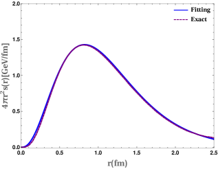
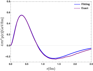
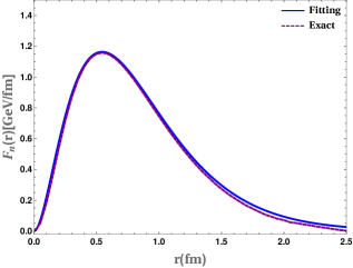
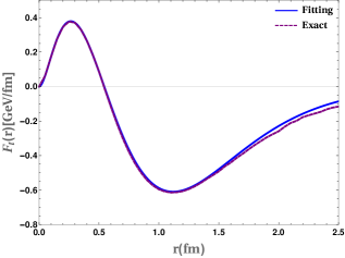
Figure 1: The solid-blue curve in the upper left panel shows the 3D shear force distribution in the Breit frame for the LFQDQ model (using the inverse Abel transformation) at the initial scale for the fitted $D(Q^{2})$ term while the purple-dashed curve is for the model data by using the Vegas. While the upper right figure draws the 3D pressure distributions. Similarly, the lower-left panel draws the 3D normal force distribution and the lower right panel draws the 3D tangential force distribution, respectively.

V DISTRIBUTIONS in three dimensions

In this section, we present the results for the 3D distributions in the Breit frame (BF). The 3D BF EMT distributions are derived from the 2D LF EMT distributions by using the inverse Abel transformationPolyakov:2007rv ; Moiseeva:2008qd .
In the left and right panels of Fig. 2, we compare the model results for the energy(mass) distributions with the Chiral quark-soliton model($\chi$QSM) Goeke:2007fp ; Kim:2021jjf for the 2D and 3D mass distributions in the LF (Drell-Yan) and BF, respectively. By using Eq.(18) we compute the 2D momentum distributions and then the 3D momentum distributions are calculated by the inverse Abel transformation defined in Eq.(19). The values of the mass distribution in the LF-frame and BF at the center of the nucleon are found to be $\mathcal{E}(0)$=1.54 GeV/$fm^{2}$ and $\epsilon(0)$=2.02 GeV/$fm^{3}$ respectively. In Fig. 2, we have shown the 2D and 3D mass distributions weighted by $2\pi x_{\perp}$ and $4\pi r^{2}$ respectively. one can see from Fig. 2 that 3D mass distribution exhibits a broader shape than the 2D mass distributions. This indicates that the 3D mass-radius Goeke:2007fp should be larger than the 2D mass-radius Kim:2021jjf . The numerical values of the mass radii for the 2D and 3D distributions are given in Table 2. The ratio between the 2D and 3D mean square mass radii in this model is found as

$$\frac{\langle x_{\perp}^{2}\rangle_{mass}}{\langle r^{2}\rangle_{mass}}=\frac{2}{3},$$ (28)

where these 2D and 3D mass radii are respectively defined as Freese:2021czn ; Goeke:2007fp ; Kim:2021jjf

$$\langle x_{\perp}^{2}\rangle_{mass}=\frac{1}{M}\int d^{2}x_{\perp}x_{\perp}^{2}\mathcal{E}(x_{\perp}),\hskip 28.45274pt\langle r^{2}\rangle_{mass}=\frac{\int d^{3}rr^{2}\epsilon(r)}{\int d^{3}r\epsilon(r)}.$$ (29)

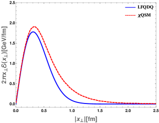
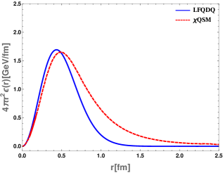
Figure 2: The solid blue curve in the left panel shows the 2D mass distribution in the LF-frame for the LFQDQ model while the red-dashed curve is the 2D mass distribution for the $\chi$QSM model Kim:2021jjf . Similarly, the solid blue curve in the right panel shows the 3D mass distribution in the BF for the LFQDQ (after doing the inverse Abel transformation) whereas the red-dashed curve is the 3D mass distribution for $\chi$QSM model Goeke:2007fp . Our model predictions are at evolved scale $\mu^{2}$=4 GeV².

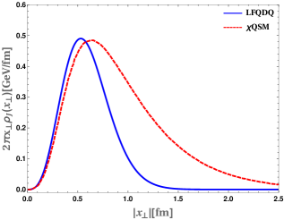
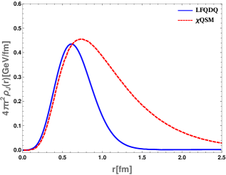
Figure 3: The solid blue curve in the left panel shows the 2D angular momentum distribution in the LF-frame for the LFQDQ model while the red-dashed curve is the 2D angular momentum distribution for the $\chi$QSM model Kim:2021jjf . Similarly, the solid blue curve in the right panel shows the 3D angular momentum distribution in the BF for the LFQDQ (after doing the inverse Abel transformation) whereas the red-dashed curve is the 3D angular momentum distribution for $\chi$QSM model Goeke:2007fp . Our model predictions are at the scale $\mu^{2}$=4 GeV².

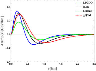
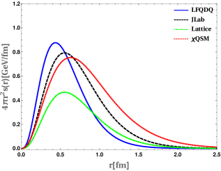
Figure 4: The solid blue, black-dashed, red-dotted, and green-dot-dashed curves in the left panel represent the 3D pressure distributions (in Breit Frame) for LFQDQ, JLab Burkert:2018bqq ; Kumericki:2019ddg , $\chi$QSM Goeke:2007fp and Lattice predictions Shanahan:2018nnv , respectively. Whereas Solid blue, black-dashed, red-dotted, and green-dot-dashed curves in the right panel show the 3D shear-force distributions in the BF for LFQDQ, JLab Burkert:2018bqq ; Kumericki:2019ddg , $\chi$QSM Goeke:2007fp and Lattice predictions Shanahan:2018nnv . Our model predictions are at the scale $\mu^{2}$=4 GeV².

In Fig. 3 the solid-blue curves in the left panel represent the 2D angular momentum distribution (weighted by $2\pi x_{\perp}$) calculated by using Eq.(16), for the LFQDQ model whereas the dashed-red curves represent the same in $\chi$QSM model. The solid-blue (dashed-red) curves in the right panel show the 3D angular momentum distribution weighted by $4\pi r^{2}$ which are computed by using the inverse Abel transform given in Eq.(20), in the LFQDQ ($\chi QSM$) model. The 2D and 3D angular-momentum distributions are normalized as

$$\int d^{2}x_{\perp}\rho^{2D}_{J}(x_{\perp})=\int d^{3}r\rho_{J}(r)=J(0)=\frac{1}{2},$$ (30)

which is related to the nucleon spin. Similar to the mass distribution, the 3D angular momentum distribution is also broader than the 2D distribution. The 2D radius Kim:2021jjf for the angular momentum distribution is related to the 3D distribution Goeke:2007fp , and is smaller than the 3D radius by a geometric factor 4/5. i.e,

$$\langle x_{\perp}^{2}\rangle_{J}\approx\frac{4}{5}\langle r^{2}\rangle_{J}$$ (31)

where these 2D and 3D angular momentum radii are defined as

$$\langle x_{\perp}^{2}\rangle_{J}=2\int d^{2}x_{\perp}x_{\perp}^{2}\rho_{J}^{(2D)}(x_{\perp}),\hskip 14.22636ptand\hskip 14.22636pt\langle r^{2}\rangle_{J}=\frac{\int d^{3}rr^{2}\rho_{J}(r)}{\int d^{3}r\rho_{J}(r)}.$$ (32)

The numerical values of these 2D and 3D angular momentum radii for the LFQDQ model are given in Table 2.

The solid-blue curve in the left(right) panel of Fig. 4 shows the 3D pressure(shear-force) distributions for the LFQDQ model, while the black-dashed, red-dotted and green-dot-dashed curves show the pressure and shear-force distributions for JLab, $\chi QSM$ and Lattice predictions, respectively. The pressure $p(r)$ has the global maximum at $r=0$, with $p(0)=4.76GeV/fm^{3}=7.62\times 10^{35}$ Pa. Which is 10-100 times higher than the pressure inside a neutron star Prakash:2000jr . The pressure decreases monotonically, becoming zero at the nodal point, $r_{0}\approx 0.43$ fm. The pressure reaches the global minimum at $r_{p,min}=0.67$ fm, after which it increases monotonically but remains negative until it goes to zero. The positive sign of the pressure for $r<r_{0}$ corresponds to the repulsion, whereas the negative sign in the region $r>r_{0}$ is for the attraction. Unlike pressure, the shear force distribution is always positive.

The conservation of the EMT currents $\partial_{\mu}\hat{T}^{\mu\nu}=0$, provides the 2D as well as 3D stability conditions. We obtain the 3D equilibrium equations from the conservation of the EMT currents, which are equivalent to the 2D stable conditions as Polyakov:2018zvc ; Kim:2021jjf ; Panteleeva:2021iip ,

$$p^{\prime}(r)+\frac{2s(r)}{r}+\frac{2}{3}s^{\prime}(r)=0\Longleftrightarrow\mathcal{P}^{\prime}(x_{\perp})+\frac{\mathcal{S}(x_{\perp})}{x_{\perp}}+\frac{1}{2}\mathcal{S}^{\prime}(x_{\perp})=0$$ (33)

From the above Eq.(33) one can easily see that the pressure and shear forces are not independent functions but due to EMT conservation, they are related to each other. Another consequence of the EMT conservation is the von Laue condition for the 2D and 3D pressure and shear forces for the nucleons Polyakov:2018zvc ,

$$\int d^{3}rp(r)=0\Longleftrightarrow\int d^{2}x_{\perp}\mathcal{P}(x_{\perp})=0$$ (34)

$$\int_{0}^{\infty}drr\left[p(r)-\frac{1}{3}s(r)\right]=0\Longleftrightarrow\int_{0}^{\infty}dx_{\perp}\left[\mathcal{P}(x_{\perp})-\frac{1}{2}\mathcal{S}(x_{\perp})\right]=0$$ (35)

From the above two Eqs. ((34),(35)) one can see that 3D von Laue conditions are satisfied if and only if the 2D ones are satisfied. By using the Eq.(33) the Druck-term can be expressed in terms of 2D and 3D pressure and force distributions as,

$$D(0)=-M\int d^{2}x_{\perp}x_{\perp}^{2}\mathcal{S}(x_{\perp})=4M\int d^{2}x_{\perp}x_{\perp}^{2}\mathcal{P}(x_{\perp})$$ (36)

and,

$$D(0)=-\frac{4}{15}M\int d^{3}rr^{2}s(r)=M\int d^{3}rr^{2}p(r)$$ (37)

respectively. It indicates that the 3D Able images of the 2D distributions show the equivalently same mechanical properties as 2D distributions.

In Refs. Lorce:2018egm ; Polyakov:2018zvc ; Perevalova:2016dln it was shown that for the local stability of the mechanical system, the 3D and 2D pressure and shear forces should satisfy the following conditions

$$\frac{2}{3}s(r)+p(r)>0,\hskip 28.45274pt{\rm and}\hskip 28.45274pt\frac{1}{2}\mathcal{S}(x_{\perp})+\mathcal{P}(x_{\perp})>0.$$ (38)

This inequalities imply that the Druck term (D-term) for any stable system must be negative, i.e., $D(0)<0$. More discussions about the local stability (Eq.(38)) can be found in Ref.Freese:2021czn , it is an interesting result that the stability condition in 3D implies the stability of the 2D mechanical system Chakrabarti:2020kdc . This allows us to connect the 3D mechanical radius to that in 2D as

$$\langle x_{\perp}^{2}\rangle_{mech}=\frac{4D(0)}{\int_{-\infty}^{0}dtD(t)}=\frac{2}{3}\langle r^{2}\rangle_{mech}$$ (39)

where the 2D mechanical radius is defined as

$$\langle x_{\perp}^{2}\rangle_{mech}=\frac{\int d^{2}x_{\perp}x^{2}_{\perp}\left(\frac{1}{2}\mathcal{S}(x_{\perp})+\mathcal{P}(x_{\perp})\right)}{\int d^{2}x_{\perp}\left(\frac{1}{2}\mathcal{S}(x_{\perp})+\mathcal{P}(x_{\perp})\right)}$$ (40)

and the mechanical radius in 3D is given by

$$\langle r^{2}\rangle_{mech}=\frac{\int d^{3}rr^{2}\left(\frac{2}{3}s(r)+p(r)\right)}{\int d^{3}r\left(\frac{2}{3}s(r)+p(r)\right)}.$$ (41)

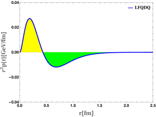
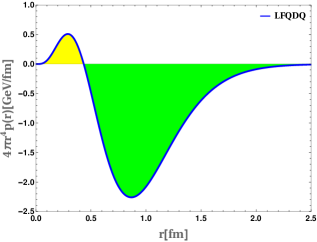
Figure 5: Left panel shows $r^{2}p(r)$ as a function of r from the LFQDQ model at evolved scale $\mu^{2}$=4 GeV². It shows how the stability condition $\int_{0}^{\infty}drr^{2}p(0)=0$ in Eq.(34) is realized. Right panel shows $4\pi r^{4}p(r)$. Note that the area under the curve is negative which implies $D<0$.

Numerical verification of the stability condition Eq.(34) is presented in Fig. 5 . The left panel in Fig. 5 shows $r^{2}p(r)$ as a function of $r$. The yellow shaded region in the positive upper half in the left panel of Fig. 5 has exactly the same surface areas as in the negative half (shaded in green). i.e.,

$$\int_{0}^{r_{0}}drr^{2}p(r)=6.74MeV,$$ (42)

$$\int_{r_{0}}^{\infty}drr^{2}p(r)=-6.74MeV$$

$$\begin{array}[]{lcccccc}\hline\cr\hline\cr\mathcal{E}(0)\left(\mathrm{GeV}/\mathrm{fm}^{2}\right)&\mathcal{P}(0)\left(\mathrm{GeV}/\mathrm{fm}^{2}\right)&\left(x_{\perp}\right)_{0}(\mathrm{fm})&\left\langle x_{\perp}^{2}\right\rangle_{\text{mass }}\left(\mathrm{fm}^{2}\right)&\left\langle x_{\perp}^{2}\right\rangle_{J}\left(\mathrm{fm}^{2}\right)&\left\langle x_{\perp}^{2}\right\rangle_{\text{mech }}\left(\mathrm{fm}^{2}\right)\\ \hline\cr 1.54&0.354&0.34&0.21&0.38&0.167\\ \hline\cr\hline\cr\varepsilon(0)\left(\mathrm{GeV}/\mathrm{fm}^{3}\right)&p(0)\left(\mathrm{GeV}/\mathrm{fm}^{3}\right)&r_{0}(\mathrm{fm})&\left\langle r^{2}\right\rangle_{\text{mass }}\left(\mathrm{fm}^{2}\right)&\left\langle r^{2}\right\rangle_{J}\left(\mathrm{fm}^{2}\right)&\left\langle r^{2}\right\rangle_{\text{mech }}\left(\mathrm{fm}^{2}\right)\\ \hline\cr 2.02&4.76&0.43&0.32&0.51&0.251\\ \hline\cr\hline\cr\end{array}$$

Table 2: Various observable obtained from the EMT distributions for the proton in both 2D LF and 3D BF are listed: the energy distributions at the nucleon center ($\mathcal{E}(0)$,$\epsilon(0)$), pressure distribution at the nucleon center ($\mathcal{P}(0)$,$p(0)$), nodal points of the pressure ($(x_{\perp})_{0}$,$r_{0}$), and the mean square radii of the mass, angular momentum and mechanical ($\langle x_{\perp}^{2}\rangle$, $\langle r^{2}\rangle$).

where $r_{0}$ is the nodal point in 3D BF, and thus they cancel each other to produce zero as required by the stability condition (Eq.(34)). In the right panel of Fig. 5 we show $4\pi r^{4}p(r)$ with $r$ which tells us about the sign of the D-term. The area in the negative half (green) is much larger than the area in the positive half (yellow). From Eq.(37) we can see that in the LFQDQ model the D-term at zero momentum transfer takes a negative value, i.e, $D(0)<0$. The same conclusion can be derived from Eq.(36) as well.

The pressure and the shear force distributions are again related to the normal(radial) and the tangential force fields, which are the eigenvalues of the stress tensor, $T_{ij}$. So, the 3D and the 2D force fields on the BF and the LF frame can be obtained as Polyakov:2018zvc ; Kim:2021jjf ,

$$F_{n}(r)=4\pi r^{2}\left[\frac{2}{3}s(r)+p(r)\right],\hskip 28.45274ptF_{t}(r)=4\pi r^{2}\left[-\frac{1}{3}s(r)+p(r)\right]$$ (43)

and,

$$F_{n}^{(2D)}(x_{\perp})=2\pi x_{\perp}\left[\frac{1}{2}\mathcal{S}(x_{\perp})+\mathcal{P}(x_{\perp})\right],\hskip 28.45274ptF_{t}^{(2D)}(x_{\perp})=2\pi x_{\perp}\left[-\frac{1}{2}\mathcal{S}(x_{\perp})+\mathcal{P}(x_{\perp})\right]$$ (44)

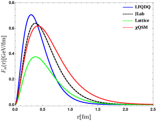
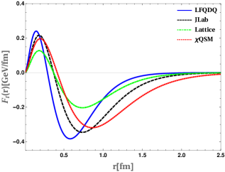
Figure 6: The solid blue, black-dashed, red-dotted and green-dot-dashed curves in the left panel represents the 3D normal force field distributions (in Breit Frame) for LFQDQ, JLab Burkert:2018bqq ; Kumericki:2019ddg , $\chi$QSM Goeke:2007fp and Lattice predictions Shanahan:2018nnv , respectively. Whereas Solid blue, black-dashed, red-dotted, and green-dot-dashed curves in the right panel show the 3D tangential force field distributions in the BF for LFQDQ, JLab Burkert:2018bqq ; Kumericki:2019ddg , $\chi$QSM Goeke:2007fp and Lattice predictions Shanahan:2018nnv , respectively. Our model predictions are at the evolved scale $\mu^{2}$=4 GeV².

respectively, In the left panel of Fig. 6 the solid blue curve depicts the 3D normal force field, while the black-dashed, red-dotted and the green-dot-dashed curves are the 3D normal force distributions for the JLab Burkert:2018bqq ; Kumericki:2019ddg , $\chi$QSM Goeke:2007fp and Lattice predictions Shanahan:2018nnv , respectively. The right panel of Fig. 6 shows the 3D tangential force field distributions for the LFQDQ (solid-blue), JLab (black-dashed) Burkert:2018bqq ; Kumericki:2019ddg , $\chi QSM$ (red-dotted) Goeke:2007fp and Lattice (green-dot-dashed) Shanahan:2018nnv , respectively. The 2D normal and tangential force field distributions for the quark- scalar-diquark model can be found in Ref.Chakrabarti:2020kdc . In a stable spherically symmetric system the normal force $F_{n}(r)$ must be a stretching force otherwise the system would squeeze and collapse to the center. Whereas, the tangential force changes its direction with the distance $r$ because the average value of possible squeezing has to be zero for a spherically symmetric system. The normal force complies with the local stability condition (38) and the tangential force satisfies the von Laue condition (34). Due to this condition, both 2D and 3D tangential forces have at least one nodal point, which tells that the direction of the force field should be reversed at this point. In the LFQDQ model the 3D and 2D tangential forces changes its direction at $r_{0}\approx 0.29$ fm and $(x_{\perp})_{0}\approx 0.20$ fm, respectively.

In Table 2, we list the numerical values for various observables such as energy and pressure densities at the center of the nucleon in both the BF and LF frames. The explicit values of the nodal points are also given. One can see from Table 2 that the magnitudes of these observables are larger in 3D BF than those in the 2D LF frame. A similar type of behavior for those observables has been also observed in Ref.Kim:2021jjf .

VI Conclusion

Of the three GFFs, Druck term or the D-term is the least understood form factor. The D-term is physically very important as it gives the shear and pressure distributions inside the proton. Recently, JLab reported the first measurement of the shear and pressure forces inside the proton and hence there are renewed interests in recent time to study the D-term in different models. Generally, the three dimensional distributions are defined in the Breit frame which are subject to relativistic corrections while in the light front the distributions are most conveniently evaluated in 2D transverse plane. Recently, it was shown that the Abel transformation relates the 2D light front distributions to the 3D distributions in the Breit frame. In this paper, the 2D LF distributions are evaluated in a quark-scalar diquark model of proton and then the 3D distributions are obtained using the Abel transformation. The wavefunctions in the model are constructed by modifying the two-particle wavefunctions predicted by AdS/QCD which can not be evaluated in perturbation theory and encode nonperturbative contributions. Our results are compared with the $\chi QSM$, JLab and lattice predictions. The 3D stability conditions translated to 2D are found to be satisfied by the 2D distributions obtained in the LFQDQ model. Various properties such as the energy and pressure distributions at the nucleon center, mass, angular momentum, mechanical radii, etc are evaluated from the EMT distributions in 2D transverse plane and the corresponding 3D distributions in the Breit frame are obtained by Abel transformations. The normal and shear force distributions are also evaluated in the LFQDQ model. Our results are found to be consistent with lattice and other model predictions.

VII Acknowledgement

This work is supported by Science and Engineering Research Board under the Grant No. CRG/2019/000895. The work of AM is supported by the SERB-POWER Fellowship (file no. SPF/2021/000102).

References

- [1] Maxim V. Polyakov and Peter Schweitzer. Forces inside hadrons: pressure, surface tension, mechanical radius, and all that. Int. J. Mod. Phys. A, 33(26):1830025, 2018.
- [2] Cédric Lorcé, Hervé Moutarde, and Arkadiusz P. Trawiński. Revisiting the mechanical properties of the nucleon. Eur. Phys. J. C, 79(1):89, 2019.
- [3] I. Yu. Kobzarev and L. B. Okun. GRAVITATIONAL INTERACTION OF FERMIONS. Zh. Eksp. Teor. Fiz., 43:1904–1909, 1962.
- [4] Heinz Pagels. Energy-Momentum Structure Form Factors of Particles. Phys. Rev., 144:1250–1260, 1966.
- [5] Maxim V. Polyakov and C. Weiss. Skewed and double distributions in pion and nucleon. Phys. Rev. D, 60:114017, 1999.
- [6] N. Kivel, Maxim V. Polyakov, and M. Vanderhaeghen. DVCS on the nucleon: Study of the twist - three effects. Phys. Rev. D, 63:114014, 2001.
- [7] Dieter Müller, D. Robaschik, B. Geyer, F. M. Dittes, and J. Hořejši. Wave functions, evolution equations and evolution kernels from light ray operators of QCD. Fortsch. Phys., 42:101–141, 1994.
- [8] Xiang-Dong Ji. Gauge-Invariant Decomposition of Nucleon Spin. Phys. Rev. Lett., 78:610–613, 1997.
- [9] A. V. Radyushkin. Scaling limit of deeply virtual Compton scattering. Phys. Lett. B, 380:417–425, 1996.
- [10] A. V. Radyushkin. Asymmetric gluon distributions and hard diffractive electroproduction. Phys. Lett. B, 385:333–342, 1996.
- [11] Abha Rajan, Tyler Gorda, Simonetta Liuti, and Kent Yagi. Bounds on the Equation of State of Neutron Stars from High Energy Deeply Virtual Exclusive Experiments. arXiv:1812.01479, 2018.
- [12] M. V. Polyakov. Generalized parton distributions and strong forces inside nucleons and nuclei. Phys. Lett. B, 555:57–62, 2003.
- [13] V. D. Burkert, L. Elouadrhiri, and F. X. Girod. The pressure distribution inside the proton. Nature, 557(7705):396–399, 2018.
- [14] V. D. Burkert, L. Elouadrhiri, and F. X. Girod. Determination of shear forces inside the proton. arXiv:2104.02031, 2021.
- [15] M. Gockeler, R. Horsley, D. Pleiter, Paul E. L. Rakow, A. Schafer, G. Schierholz, and W. Schroers. Generalized parton distributions from lattice QCD. Phys. Rev. Lett., 92:042002, 2004.
- [16] Philipp Hagler, John W. Negele, Dru Bryant Renner, W. Schroers, T. Lippert, and K. Schilling. Moments of nucleon generalized parton distributions in lattice QCD. Phys. Rev. D, 68:034505, 2003.
- [17] P. E. Shanahan and W. Detmold. Pressure Distribution and Shear Forces inside the Proton. Phys. Rev. Lett., 122(7):072003, 2019.
- [18] Marina Dorati, Tobias A. Gail, and Thomas R. Hemmert. Chiral perturbation theory and the first moments of the generalized parton distributions in a nucleon. Nucl. Phys. A, 798:96–131, 2008.
- [19] Jiunn-Wei Chen and Xiang-dong Ji. Leading chiral contributions to the spin structure of the proton. Phys. Rev. Lett., 88:052003, 2002.
- [20] Andrei V. Belitsky and X. Ji. Chiral structure of nucleon gravitational form-factors. Phys. Lett. B, 538:289–297, 2002.
- [21] M. Diehl, A. Manashov, and A. Schafer. Generalized parton distributions for the nucleon in chiral perturbation theory. Eur. Phys. J. A, 31:335–355, 2007.
- [22] K. Goeke, J. Grabis, J. Ossmann, M. V. Polyakov, P. Schweitzer, A. Silva, and D. Urbano. Nucleon form-factors of the energy momentum tensor in the chiral quark-soliton model. Phys. Rev. D, 75:094021, 2007.
- [23] June-Young Kim and Hyun-Chul Kim. Energy-momentum tensor of the nucleon on the light front: Abel tomography case. Phys. Rev. D, 104(7):074019, 2021.
- [24] C. Cebulla, K. Goeke, J. Ossmann, and P. Schweitzer. The Nucleon form-factors of the energy momentum tensor in the Skyrme model. Nucl. Phys. A, 794:87–114, 2007.
- [25] Hyun-Chul Kim, Peter Schweitzer, and Ulugbek Yakhshiev. Energy-momentum tensor form factors of the nucleon in nuclear matter. Phys. Lett. B, 718:625–631, 2012.
- [26] Adam Freese and Gerald A. Miller. Forces within hadrons on the light front. Phys. Rev. D, 103:094023, 2021.
- [27] Julia Yu. Panteleeva and Maxim V. Polyakov. Forces inside the nucleon on the light front from 3D Breit frame force distributions: Abel tomography case. Phys. Rev. D, 104(1):014008, 2021.
- [28] Dipankar Chakrabarti, Chandan Mondal, Asmita Mukherjee, Sreeraj Nair, and Xingbo Zhao. Gravitational form factors and mechanical properties of proton in a light-front quark-diquark model. Phys. Rev. D, 102:113011, 2020.
- [29] Thomas Gutsche, Valery E. Lyubovitskij, Ivan Schmidt, and Alfredo Vega. Light-front quark model consistent with Drell-Yan-West duality and quark counting rules. Phys. Rev. D, 89(5):054033, 2014. [Erratum: Phys.Rev.D 92, 019902 (2015)].
- [30] Stanley J. Brodsky and Susan Gardner. Evidence for the Absence of Gluon Orbital Angular Momentum in the Nucleon. Phys. Lett. B, 643:22–28, 2006.
- [31] Dipankar Chakrabarti and Chandan Mondal. Chiral-odd generalized parton distributions for proton in a light-front quark-diquark model. Phys. Rev. D, 92(7):074012, 2015.
- [32] Guy F. de Teramond and Stanley J. Brodsky. Hadronic Form Factor Models and Spectroscopy Within the Gauge/Gravity Correspondence. In Ferrara International School Niccolò Cabeo 2011: Hadronic Physics, pages 54–109, 2011.
- [33] Xiangdong Ji, Xiaonu Xiong, and Feng Yuan. Transverse Polarization of the Nucleon in Parton Picture. Phys. Lett. B, 717:214–218, 2012.
- [34] A. Harindranath, Rajen Kundu, and Asmita Mukherjee. On transverse spin sum rules. Phys. Lett. B, 728:63–67, 2014.
- [35] Krešimir Kumerički. Measurability of pressure inside the proton. Nature, 570(7759):E1–E2, 2019.
- [36] M. V. Polyakov. Tomography for amplitudes of hard exclusive processes. Phys. Lett. B, 659:542–550, 2008.
- [37] Alena M. Moiseeva and Maxim V. Polyakov. Dual parameterization and Abel transform tomography for twist-3 DVCS. Nucl. Phys. B, 832:241–250, 2010.
- [38] Cédric Lorcé, Luca Mantovani, and Barbara Pasquini. Spatial distribution of angular momentum inside the nucleon. Phys. Lett. B, 776:38–47, 2018.
- [39] Dipankar Chakrabarti, Chandan Mondal, and Asmita Mukherjee. Gravitational form factors and transverse spin sum rule in a light front quark-diquark model in AdS/QCD. Phys. Rev. D, 91(11):114026, 2015.
- [40] Dipankar Chakrabarti, Chandan Mondal, Asmita Mukherjee, Sreeraj Nair, and Xingbo Zhao. Proton gravitational form factors in a light-front quark-diquark model. In 28th International Workshop on Deep Inelastic Scattering and Related Subjects, 8 2021.
- [41] Yuri L. Dokshitzer. Calculation of the Structure Functions for Deep Inelastic Scattering and e+ e- Annihilation by Perturbation Theory in Quantum Chromodynamics. Sov. Phys. JETP, 46:641–653, 1977.
- [42] V. N. Gribov and L. N. Lipatov. Deep inelastic e p scattering in perturbation theory. Sov. J. Nucl. Phys., 15:438–450, 1972.
- [43] Guido Altarelli and G. Parisi. Asymptotic Freedom in Parton Language. Nucl. Phys. B, 126:298–318, 1977.
- [44] Gavin P. Salam and Juan Rojo. A Higher Order Perturbative Parton Evolution Toolkit (HOPPET). Comput. Phys. Commun., 180:120–156, 2009.
- [45] Ph. Hagler et al. Nucleon Generalized Parton Distributions from Full Lattice QCD. Phys. Rev. D, 77:094502, 2008.
- [46] Krešimir Kumerički and Dieter Müller. Description and interpretation of DVCS measurements. EPJ Web Conf., 112:01012, 2016.
- [47] B. Pasquini, M. V. Polyakov, and M. Vanderhaeghen. Dispersive evaluation of the D-term form factor in deeply virtual Compton scattering. Phys. Lett. B, 739:133–138, 2014.
- [48] Xiang-Dong Ji, W. Melnitchouk, and X. Song. A Study of off forward parton distributions. Phys. Rev. D, 56:5511–5523, 1997.
- [49] G. Peter Lepage. A New Algorithm for Adaptive Multidimensional Integration. J. Comput. Phys., 27:192, 1978.
- [50] G. Peter Lepage. Adaptive multidimensional integration: VEGAS enhanced. J. Comput. Phys., 439:110386, 2021.
- [51] Madappa Prakash, James M. Lattimer, Jose A. Pons, Andrew W. Steiner, and Sanjay Reddy. Evolution of a neutron star from its birth to old age. Lect. Notes Phys., 578:364–423, 2001.
- [52] I. A. Perevalova, M. V. Polyakov, and P. Schweitzer. On LHCb pentaquarks as a baryon-(2S) bound state: prediction of isospin- pentaquarks with hidden charm. Phys. Rev. D, 94(5):054024, 2016.