Computational Complexity Evaluation of Neural Network Applications in Signal Processing

Abstract

In this paper, we provide a systematic approach for assessing and comparing the computational complexity of neural network layers in digital signal processing. We provide and link four software-to-hardware complexity measures, defining how the different complexity metrics relate to the layers’ hyper-parameters. This paper explains how to compute these four metrics for feed-forward and recurrent layers, and defines in which case we ought to use a particular metric depending on whether we characterize a more soft- or hardware-oriented application. One of the four metrics, called ‘the number of additions and bit shifts (NABS)’, is newly introduced for heterogeneous quantization. NABS characterizes the impact of not only the bitwidth used in the operation but also the type of quantization used in the arithmetical operations. We intend this work to serve as a baseline for the different levels (purposes) of complexity estimation related to the neural networks’ application in real-time digital signal processing, aiming at unifying the computational complexity estimation.

I Introduction

Over the last few decades, neural networks (NNs) have begun to find widespread usage in a wide range of signal processing applications: filtering, parameter estimation, signal detection, system identification, pattern recognition, signal reconstruction, time series analysis, signal compression, signal transmission, etc. [1, 2, 3, 4]. Audio, video, image, communication, geophysical and radar scanning data, are the examples of important signal types that typically undergo various forms of signal processing [5, 6, 7]. The key capabilities of NNs in signal processing are: performing distributed processing, emulating nonlinear transformations and processes, self-organizing, and enabling high-speed processing communication applications[8, 9, 10] . With these properties, NNs can provide a very powerful means of solving many signal processing tasks, particularly in the areas related to the nonlinear signal processing, real-time signal processing, adaptive signal processing, and blind signal processing [11, 5, 12, 13].

Real-time signal processing, as an example, is a field that enables technological breakthroughs by effectively incorporating signal processing in hardware: real-time and onboard signal processing is the key to the evolution of phones and watches into smartphones/smartwatches. To the best of our knowledge, one of the first real-time applications of NNs was discussed in 1989  [14], and numerous works since then have deliberated the challenges of implementing such solutions in hardware exploiting the notion of computational complexity [15, 16, 17, 18, 19, 20, 21, 22, 23, 24].

From a computer science perspective, computational complexity analysis is almost always attributed to the Big-$O$ notation of the algorithm [25, 26, 27]. In general, the Big-$O$ notation is used to express an algorithm’s complexity while assessing its efficiency, which means that we are interested in how effectively the algorithm scales with the size of the dataset in terms of running time [28, 29, 30]. However, from the engineering standpoint, the Big-$O$ is often an oversimplified measure that cannot be immediately translated into the hardware resources required to realize the algorithm (NNs) in a hardware platform [16].

Due to this problem that refers to the absence of some “universal” measure, various works started to present complexity in terms of multiply and accumulate (MAC) [15, 16, 17, 18], Kolmogorov complexity [19], the number of bit-operations (BOP) [20, 21], the number of real multiplications (RM) [22, 23, 24]. However, it is not always clear when to use each specific metric, and, more importantly, none of the metrics mentioned above shows the benefits of using different strategies of quantization for saving the complexity of implementing the multipliers.

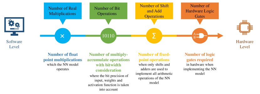
Figure 1: Diagram of computational complexity metrics illustrating the various levels of complexity measurement from software to hardware.

As far as we know, no work has so far unified the computational metrics itemized above such that we have no universal metrics to compare the complexity when different types of quantization are applied for NN structures. In this paper, we solve this issue by carrying out a systematic computational complexity analysis for a zoo of NN layer types. In addition, we introduce a new useful metric: we coined ‘the number of additions and bit shifts’ (NABS). This metric takes into account the impact of the weights’ quantization type on the reduction of the multipliers’ implementation complexity used in an NN layer. Overall, we intend our work to give largely universal measures of complexity to establish a comparison baseline depending on whether the application is software- or hardware-based.

The paper is organized as follows. In Sec. II we describe the details of different computational metrics from soft- and hardware implementation levels. Sec. III presents how to compute the computational complexity of different NN layers. Sec. IV describes the results of our evaluation of how complexity grows against the design parameters of each NN layer. We also address the impact of quantization on different computational complexity metrics. Our findings are summarized in the conclusion.

II Four Metrics of Computational Complexity

Accurate computational complexity evaluation is critical in the design of digital signal processing (DSP) devices to better understand the implementation feasibility and bottlenecks for each device’s structure. With this in mind, we summarize the four most commonly used different criteria for assessing the computational complexity, from the software level to the hardware level, in Fig. 1.

The first, most software-oriented, level of estimation traditionally deals only with counting the number of real multiplications of the algorithm [31, 32] (quite often defined per one processed element, say a sample or a symbol). This metric is the number of real multiplications (RM). When comparing computational complexity, the purpose of this high-level metric is to consider only the multipliers required, ignoring additions, because the implementation of the latter in hardware or software is initially considered cheap, while the multiplier is generally the slowest element in the system and consumes the largest chip area [33, 31]. This ignoring the additions can also be easily understood by looking at the Big-$O$ analysis of multiplier versus adder. When multiplying two integers with $n$ digits, the computational complexity of the multiplication instance is $O(n^{2})$, whereas the addition of the same two numbers has a computational complexity of $\Theta(n)$ [34]. As a result, if you are dealing with float values with 16 decimal digits, multiplication is by far the most time-consuming part of the implementation procedure. Therefore, when comparing solutions that use floating-point arithmetic with the same bitwidth precision, the RM metric provides an acceptable comparative estimate to qualitatively assess the complexity against some existing benchmarks (e.g. against the DSP operations for optical channel equalization tasks [32]).

When moving to fixed-point arithmetic, the second metric known as the number of bit-operations (BOP) must be adopted to understand the impact of changing the bitwidth precision on the complexity. The BOP metric provides a good insight into mixed-precision arithmetic performance, since we can forecast the BOP needed for fundamental arithmetic operations like addition and multiplication, given the bitwidth of two operands. In a nutshell, the BOP metric aims to generalize floating-point operations (FLOPs) to heterogeneously quantized NNs, as far as the FLOPs cannot be efficiently used to evaluate integer arithmetic operations [21, 35]. For the BOP metric, we have to include the complexity contribution of both multiplications and additions, since now we evaluate the complexity in terms of the most common operations in NNs: the multiply-and-accumulate operations (MACs) [21, 35, 36]. However, the BOP accounts for the scaling of the number of multipliers with the bitwidth of two operands, and the scaling of the number of adders with the accumulator bitwidth. Note that since most real DSP implementations use dedicated logic macros (e.g. DSP slice in Field Programmable Gate Arrays [FPGA] or MAC in Application Specific Integrated Circuit [ASIC]), the BOP metric fits as a good complexity estimation metric inasmuch as the BOP also accesses the MAC taking into account the particular bitwidth of two operands.

TABLE I: Capacity ranges for XC4000 Series CLB Resources given in Ref. [37].

CLB Resource	Logic Gate Range
Gate range per 4-input LUT (2 per CLB)	1 to 9
Gate range per 3-input LUT	1 to 6
Gate range per flip-flop (2 per CLB)	6 to 12
Total gate range per CLB	15 to 48
Estimated typical number of gates per CLB	28.5

The progress in the development of new advanced NN quantization techniques [38, 39, 40, 41] allowed implementing the fixed point multiplications participating in NNs efficiently, namely with the use of a few bit-shifters and adders [42, 43, 44]. Since the BOP lacks the ability to properly assess the effect of different quantization strategies on the complexity, a new, more sophisticated metric is required there. We introduce the third complexity metric that counts the number of total equivalent additions to represent the multiplication operation, called the number of additions and bit shifts (NABS). The number of shift operations can be neglected when calculating the computational complexity because, in the hardware, the shift can be performed without extra costs in constant time with the $O(1)$ complexity. Even though the cost of bit shifts can be ignored due to the aforementioned reasons, and only the total number of adders has to be accounted for to measure the computational complexity, we prefer to keep the full name “number of additions and bit shifts” to highlight that the multiplication is now represented as shifts and adders.

Finally, the metric which is closest to the hardware level is the number of logic gates (NLG) that is used for our evaluating method’s hardware (e.g. ASIC or FPGA) implementation. It is different from the NABS metric, as now the true cost of implementation is to be presented. In this case, the activation function cost, represented by look-up tables (LUT) is also taken into account. Additionally, other metrics like the number of flip-flops (FFs) or registers, the number of logic blocks used for general logic and memory blocks, or other special functional macros used in the design, are also relevant. As it is clear from this explanation, there will be no straightforward equation to convert the NABS to NLG as the latter depends on the circuit design adopted by the developer. Tools such as Synopsys Synthesis [45] for ASIC implementation can provide this kind of information. However, with regard to the FPGA design, it is harder to get a correct estimate of the gate count from the report of the FPGA tools [46].

In this paper, we advocate that the NLG metric should be applied to count the number of logic gates used to implement the hardware piece, similar to the concept of the Maximum Logic Gates metric for FPGA devices [37]. The Maximum Logic Gates metric is utilized to approximate the maximum number of gates that can be realized in the FPGA for a design consisting of only logic functions. Additionally, this metric is based on an estimate of the typical number of usable gates per configurable logic block (CLB) or logic cell multiplied by the total number of such blocks or cells [37]. With regard to the correspondence between CLB and logic gates number, see Table I.

It should be noted that Table I is based on an older, now obsolete, 4-input LUT architecture [37]. Newer FPGA families now feature a 6-input LUT architecture, and to address the resource consumption for the new generation of devices, a reasonable approximation would be to increase the ‘maximum gate range equivalent per LUT’ figure used in [37] by 50%. Note that the gate equivalence figures for FF’s (registers) still hold true for the 6-input architecture. It is also worth noting that the CLB architecture has changed substantially since Ref. [37] was published, such that we include Table II linking CLB-gates with more up-to-date 6-input architecture.

TABLE II: Estimated capacity ranges for 6 input LUT based CLB Resources.

CLB Resource	Logic Gate Range
Gate range per 6-input LUT (8 per CLB)	6 to 15
Gate range per flip-flop (16 per CLB)	6 to 12
Total gate range per CLB	144 to 312

To conclude, we comment on universal metrics between the FPGA and the ASIC implementations. We emphasize that calculating an ASIC gate equivalent to an FPGA DSP slice is not a straightforward task because not all features are necessarily required when implementing the specific arithmetic function in an ASIC. However, utilizing the estimation approach laid out in Ref. [37], a figure can be obtained. Using the Xilinx Ultrascale + DSP48E2 slice basic multiplier functionality as an example (see Xilinx UG579 Fig. 1-1 in Ref. [47]) and pipelining it for maximum performance, it is possible to estimate the number of FFs and adders required for such an ASIC equivalence. Taking into account the structure of the multiplication of a $m$-bit number by a $n$-bit number, implemented using an array multiplier architecture, it is equivalent to $m\times n$ AND gates, $n$ half adders, and $(m-2)\times n$ full adders. For example, the ASIC equivalence of a 27$\times$18 multiplier in an FPGA would have 486 AND gates, 18 half adders, 450 full adders, and 90 Flip Flops.

III Mathematical Complexity Formulation

In this section, we provide a brief introduction to various types of NN: dense layer, Convolutional Neural Networks (CNN), Vanilla Recurrent Neural Networks (RNN), Long Short-Term Memory Neural Networks (LSTM), Gated Recurrent Units (GRU), and Echo State Networks (ESN). We investigate the computational complexity for each network in terms of RM, BOP and NABS. In this work, the computational complexity is formulated per layer, and the output layer is not taken into account for the complexity calculation to eliminate redundant computations if multiple layers or multiple NN types are combined. Table III in the section’s end summarizes the formulas for the RM, BOP, and NABS for all NN types studied.

III-A Dense Layer

A dense layer, also known as a ‘fully connected layer’, is a layer in which each neuron is connected with all the neurons from the previous layer with a specific weight $w_{{i}{j}}$. The input vector is mapped to the output vector in a nonlinear manner by the dense layer, due to the participation of a non-linear activation function. Dense layers can be combined to form a Multi-Layer Perceptron (MLP), which is a class of a feed-forward deep NN.

The output vector $y$ of a dense layer given $x$ as an input vector, is written as:

$$y=\phi(Wx+b),$$ (1)

where $y$ is the output vector, $\phi$ is a nonlinear activation function, $W$ is the weight matrix, and $b$ is the bias vector. Writing explicitly the matrix operation inside the activation function:

$$\begin{split}Wx+b=\begin{bmatrix}w_{11}&w_{12}&\ldots&w_{1n_{i}}\\ w_{21}&w_{22}&\ldots&w_{2n_{i}}\\ \vdots&\vdots&\ldots&\vdots\\ w_{n_{n}1}&w_{n_{n}2}&\ldots&w_{{n_{n}}{n_{i}}}\\ \end{bmatrix}\begin{bmatrix}x_{1}\\ \!x_{2}\\ \vdots\\ x_{n_{i}}\end{bmatrix}\;+\;\begin{bmatrix}b_{1}\\ b_{2}\\ \vdots\\ b_{n_{n}}\end{bmatrix}\!,\end{split}$$ (2)

where $n_{i}$ is the number of features in the input vector and $n_{n}$ represents the number of neurons in the layer, we can readily see that the RM of a dense layer can be computed according to the simple well-known formula:

$$\text{RM}_{\text{Dense}}=n_{n}n_{i}.$$ (3)

Now we calculate the BOP of a dense layer, taking into account the bitwidth of two operands, to approximate the computational complexity of NNs when the mixed-precision arithmetic is used. The bitwidth, also known as the precision, is the number of bits used to represent a certain element; for example, each weight in the weight matrix can be represented with $b_{w}$ bits. Fig. 2 illustrates the data flow of the MAC operations for a neuron of a dense layer with $n_{i}$ input features and $b_{i}$ as input bitwidth. The multiplication of the input vector and the weights for one neuron can be mathematically represented as follows:

$$y_{\text{MUL, one neuron}}=\sum_{n=1}^{n_{i}}w_{n}x_{n}.$$ (4)

Initially, the $n_{i}$ multiplications of input vector elements and weights for one neuron take place. When the multiplication of two operands is performed, the resulting bitwidth is the sum of the bitwidths of two operands ($b_{w}+b_{i}$) as it is shown in the first row of Fig. 2.

After that, $n_{i}-1$ additions need to be made, and the resulting number of bits can be defined as follows. Considering that the result of the addition of two operands has the bitwidth of the bigger operand plus one bit, we start adding the multiplication results pairwise until only one element remains. In this case, the second row of Fig. 2 shows the first level of pairwise additions, with resulting bitwidth of $b_{w}+b_{i}+1$, and since this pairwise addition process is repeated for $\lceil\log_{2}(n_{i})\rceil$ levels (until we have just a final single number), the total bitwidth of it is given by $b_{w}\!+\!b_{i}+\lceil\log_{2}(n_{i})\rceil$, i.e. it is the bitwidth required to perform the overall MAC process. Then, the addition of the bias vector is performed. In this work, for all types of networks, we assume that the size of the accumulator defined by the multiplication of the weight matrix and the input vector, is dominant; thereby, the assumption for the bias bitwidth $b_{b}$ is as follows: $b_{b}<b_{w}+b_{i}+\lceil\log_{2}(n_{i})\rceil$, and the addition of bias, in the end, will not result in the overflow. Finally, the bitwidth of the resulting number is truncated to $b_{a}$, where $b_{a}$ is the bitwidth of the activation function [16].

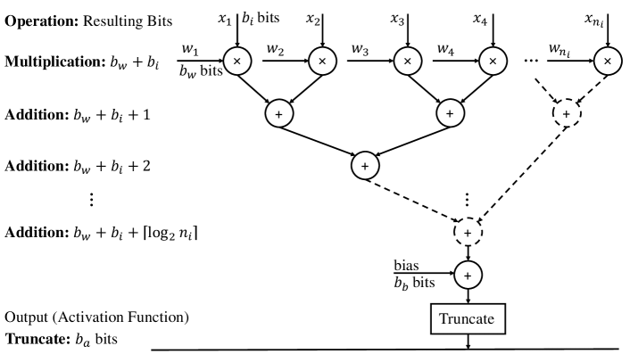
Figure 2: Data path of a neuron in a quantized dense layer where $x$ is the input vector with size $n_{i}$, $w$ is the weight matrix, $b_{w}$ is the weight bitwidth and $b_{i}$ is the input bitwidth, $b_{a}$ is the activation bitwidth and $b_{b}$ is the bias bitwidth.

When calculating the BOP for a dense layer, the costs of both multiplications and additions need to be included. Then, the BOP formula takes the form of the sum of two constituents, $\mathrm{BOP}_{\text{Mul}}$ and $\mathrm{BOP}_{\text{Bias}}$, corresponding to vector-matrix multiplication and bias addition:

$$\mathrm{BOP}_{\text{Mul}}=n_{n}\big{[}n_{i}b_{w}b_{i}+(n_{i}-1)(b_{w}+b_{i}+\lceil\log_{2}(n_{i})\rceil)\big{]},$$ (5)

$$\mathrm{BOP}_{\text{Bias}}\approx n_{n}(b_{w}+b_{i}+\lceil\log_{2}(n_{i})\rceil).$$ (6)

Eq. (5) shows the cost of the number of one-bit full adders calculated from the dot product of $n_{i}$-dimensional input vector and weight matrix, as in Refs. [21, 48]. The cost takes into account the bitwidths of the weights and input, $b_{w}$ and $b_{i}$. To compute the product of the two operands, we have to use $n_{i}n_{n}$ multiplications and $n_{n}(n_{i}-1)$ additions. The multiplication cost can be calculated by the number of multiplications multiplied by $b_{w}b_{i}$, which is related to the bit operation, and the number of additions multiplied by the accumulator bitwidth required to do the operation. The final BOP is the contribution of multiplication and the addition of bias of the dense layer. For the convenience of the forthcoming presentation, let us define the short notations:

$$\text{Mult}(n_{i},b_{w},b_{i})=n_{i}b_{w}b_{i}+(n_{i}\!-\!1)\big{(}b_{w}\!+\!b_{i}\!+\lceil\log_{2}(n_{i})\!\rceil\big{)},$$

and

$$\text{Acc}(n_{i},b_{w},b_{i})=b_{w}+b_{i}+\lceil\log_{2}(n_{i})\rceil.$$

The Acc expression represents the actual bitwidth of the accumulator required for MAC operation, as shown in Fig. 2. Then, the BOP of the dense layer expressed through the layer parameters becomes:

$$\begin{split}\mathrm{BOP}_{\text{Dense}}={}&\text{BOP}_{\text{Mul}}+\text{BOP}_{\text{Bias}}\\ \approx{}&n_{n}n_{i}\big{[}b_{w}b_{i}+(b_{w}+b_{i}+\lceil\log_{2}(n_{i})\rceil)\big{]}\\ \approx{}&n_{n}n_{i}\big{[}b_{w}b_{i}+\text{Acc}(n_{i},b_{w},b_{i})\big{]}.\end{split}$$ (7)

Now, we note that with the advancement in NN quantization techniques, there arises the opportunity to approximate multiplication by using shift and few add operations only while still maintaining a good processing accuracy, since the NNs can diminish the approximation error that the quantized approximation introduces [49, 43]. As mentioned in Sec. II, the number of shifts can be neglected compared to the contribution of adders. The number of adders is different for different types of quantization. To be more specific, let $X$ represent the number of adders required, at most, to perform the multiplication and let $b$ be the bitwidth of the quantized matrix. For uniform quantization, we have: $X=b-1$. And, for example, when the weight matrix with bitwidth of $b_{w}$, is quantized, we have $X_{w}=b_{w}-1$ as the number of adders we need at most to perform the multiplication of the weights . In the case of Power-of two (PoT) quantization, we have: $X=0$, because each multiplication costs just a shift [42, 53]. Lastly, for the Additive Powers-of-Two (APoT) quantization, we have: $X=n$, where $n$ denotes the number of additive terms. In APoT, the sum of $n$ PoT terms is used to represent each quantization level [38]. Eventually, the NABS of a dense layer can be derived from its BOP equation, Eq. (7):

$$\begin{split}\mathrm{NABS_{Dense}}\approx{}&n_{n}n_{i}\big{[}X_{w}\text{Acc}(n_{i},b_{w},b_{i})\!+\!\text{Acc}(n_{i},b_{w},b_{i})\big{]}\\ \approx{}&n_{n}n_{i}(X_{w}+1)\text{Acc}(n_{i},b_{w},b_{i}).\end{split}$$ (8)

As in Eq. (8), the multiplication term $b_{w}b_{i}$ in Eq. (7) is converted into the number of adders needed to operate the multiplication times the accumulator bitwidth required: $X_{w}\text{Acc}(n_{i},b_{w},b_{i})$.

III-B Convolutional Neural Networks

In CNN, we apply the convolutions with different filters to extract the features and convert them into a lower-dimensional feature set, but still preserve the original properties. CNNs can be used in 1D, 2D, or 3D networks depending on the applications. In this paper, we focus on 1D-CNNs, which are applicable to processing sequential data [3]. For simplicity of understanding, the 1D-CNN processing with padding equal to 0, dilation equal to 1, and stride equal to 1, can be summarized as follows:

$$y^{f}_{i}=\phi\left(\sum_{n=1}^{n_{i}}\sum_{j=1}^{n_{k}}x^{in}_{i+j-1,n}\cdot k^{f}_{j,n}+b^{f}\right),$$ (9)

where $y^{f}_{i}$ denotes the output, known as a feature map, of a convolutional layer built by the filter $f$ in the $i$-th input element, $n_{k}$ is the kernel size, $n_{i}$ is the size of the input vector, $x^{in}$ represents the raw input data, $k^{f}_{j}$ denotes the $j$-th trainable convolution kernel of the filter $f$ and $b^{f}$ is the bias of the filter $f$.

In the general case, when designing the CNN, the parameters like padding, dilation, and stride also affect the output size of the CNN. It can be formularized as:

$$OutputSize=\!\left[\frac{n_{s}+2\,padding\!-\!dilation(n_{k}-1)\!-\!1}{stride}\!+\!1\right]\!,$$ (10)

where $n_{s}$ is the input time sequence size.

The RM of a 1D-convolutional layer can be computed as follows:

$$\mathrm{RM}_{\text{CNN}}=n_{f}n_{i}n_{k}\cdot OutputSize,$$ (11)

where $n_{f}$ is the number of filters, also known as the output dimension. As in Eq. (11), there are $n_{i}n_{k}$ multiplications per sliding window, and the number of times that sliding window process needs to be repeated is equal to the output size. Then, the procedure is executed repeatedly for all $n_{f}$ filters.

The BOP for a 1D-convolutional layer, after taking into consideration the multiplications and additions, can be represented as:

$$\begin{split}\mathrm{BOP}_{\text{CNN}}={}&OutputSize\cdot n_{f}\text{Mult}(n_{i}n_{k},b_{w},b_{i})\\ +{}&n_{f}\text{Acc}(n_{i}n_{k},b_{w},b_{i}).\end{split}$$ (12)

Eq. (12) is derived from Eq. (9) and Eq. (11). The first term is associated with the convolution operation between the flattened input vector and the sliding windows, and the latter term corresponds to the addition of the bias.

The procedure to derive the NABS is similar to that described in details in the case of a dense layer, Sec. III-A. The NABS of a 1D-convolutional layer is given by:

$$\begin{split}\mathrm{NABS_{CNN}}={}&OutputSize\cdot n_{f}\big{[}n_{i}n_{k}(X_{w}+1)-1\big{]}\\ {}&\cdot\text{Acc}(n_{i}n_{k},b_{w},b_{i})\\ +{}&n_{f}\text{Acc}(n_{i}n_{k},b_{w},b_{i}).\\ \end{split}$$ (13)

To obtain the 1D-convolutional layer’s NABS, the multiplication in Eq. (12) is represented by the number of adders required, at most, to perform the multiplication times the accumulator bitwidth.

III-C Vanilla Recurrent Neural Networks

Vanilla RNN is different from MLP and CNN in terms of its ability to handle the memory, which is quite beneficial for time series data. RNNs take into account the current input and the output that the network has learned from the prior input. Even though the RNNs introduced the efficient memory handling, it still suffers from the inability to capture the long-term dependencies because of the vanishing gradient issue [54]. The equations for the vanilla RNN given a time step $t$ are as follows:

$$\begin{gathered}h_{t}=\phi(W{x}_{t}+Uh_{t-1}+b),\\ \end{gathered}$$ (14)

where $\phi$ is, again, the nonlinear activation functions, $x_{t}\in\mathbb{R}^{n_{i}}$ is the $n_{i}$-dimensional input vector at time $t$, $h_{t}\in\mathbb{R}^{n_{h}}$ is a hidden layer vector of the current state with size $n_{h}$, $W\in\mathbb{R}^{n_{h}\times n_{i}}$ and $U\in\mathbb{R}^{n_{h}\times n_{h}}$ represent the trainable weight matrices, and $b$ is the bias vector. For more explanations on the vanilla RNN operation, see Ref. [55]. The RM of a vanilla RNN is:

$$\mathrm{RM}_{\text{RNN}}=n_{s}n_{h}(n_{i}+n_{h}),$$ (15)

where $n_{h}$ notes the number of hidden units. From Eq. (15), the RM for a time step is $n_{h}(n_{i}+n_{h})$. It can be separated into two terms; the $n_{h}n_{i}$ term corresponds to the multiplication of the input vector $x_{t}$ and the weight matrix, and the $n_{h}^{2}$ term arises because of the multiplication to the prior cell output $h_{t-1}$. Finally, $n_{s}$, which denotes the number of time steps in the layer, should be taken into account, as the process is repeated $n_{s}$ times.

The BOP for a vanilla RNN is given as:

$$\begin{split}\mathrm{BOP}_{\text{RNN}}={}&n_{s}n_{h}\text{Mult}(n_{i},b_{w},b_{i})\\ +{}&n_{s}n_{h}\text{Mult}(n_{h},b_{w},b_{a})\\ +{}&2n_{s}n_{h}\text{Acc}(n_{h},b_{w},b_{a}).\end{split}$$ (16)

From Eq. (16), the first term is associated with the input vector multiplied by the weight matrix, and the second term corresponds to the multiplications of the recurrent cell outputs. The final term is the contribution of the addition between $W{x}_{t}+Uh_{t-1}$ and the addition of the bias vector in Eq. (14); one can see that the size of the accumulator used in this term, is $\text{Acc}(n_{h},b_{w},b_{a})$. It is due to the assumption that $\text{Acc}(n_{h},b_{w},b_{a})$ is dominant because it should be greater than $\text{Acc}(n_{i},b_{w},b_{i})$ as a result of the inequality $n_{h}>n_{i}$.

As in the case of a dense layer, the NABS of vanilla RNN can be calculated from its BOP equation by converting the multiplication to the number of adders needed at most ($X$) depending on the quantization scheme and the accumulator size:

$$\begin{split}\mathrm{NABS_{RNN}}={}&n_{s}n_{h}\big{[}n_{i}(X_{w}+1)-1\big{]}\text{Acc}(n_{i},b_{w},b_{i})\\ +{}&n_{s}n_{h}\big{[}n_{h}(X_{w}+1)+1\big{]}\text{Acc}(n_{h},b_{w},b_{a}).\end{split}$$ (17)

III-D Long Short-Term Memory Neural Networks

LSTM are an advanced type of RNNs. Although RNNs suffer from short-term memory issues, the LSTM network has the ability to learn long-term dependencies between time steps ($t$), insofar as it was specifically designed to address the gradient issues encountered in RNNs [56, 57]. There are three types of gates in an LSTM cell: an input gate ($i_{t}$), a forget gate ($f_{t}$), and an output gate ($o_{t}$). More importantly, the cell state vector ($C_{t}$) was proposed as a long-term memory to aggregate the relevant information throughout the time steps. The equations for the forward pass of the LSTM cell given a time step $t$ are as follows:

$$\begin{gathered}i_{t}=\sigma(W^{i}{x}_{t}+U^{i}{h}_{t-1}+b^{f}),\\ f_{t}=\sigma(W^{f}{x}_{t}+U^{f}{h}_{t-1}+b^{i}),\\ o_{t}=\sigma(W^{o}{x}_{t}+U^{o}{h}_{t-1}+b^{o}),\\ C_{t}=f_{t}\odot C_{t-1}+i_{t}\odot\phi(W^{c}{x}_{t}+U^{c}{h}_{t-1}+b^{c}),\\ h_{t}=o_{t}\odot\phi(C_{t}),\end{gathered}$$ (18)

where $\phi$ is usually the “tanh” activation functions, $\sigma$ is usually the sigmoid activation function, the sizes of each variable are $x_{t}\in\mathbb{R}^{n_{i}}$, $f_{t},i_{t},o_{t}\in(0,1)^{n_{h}}$, $C_{t}\in\mathbb{R}^{n_{h}}$ and $h_{t}\in(-1,1)^{n_{h}}$. The $\odot$ symbol represents the element-wise (Hadamard) multiplication.

The RM of a LSTM layer is:

$$\mathrm{RM}_{\text{LSTM}}=n_{s}n_{h}(4n_{i}+4n_{h}+3),$$ (19)

where $n_{h}$ is the number of hidden units in the LSTM cell. Similarly to RNNs, the RM can be calculated from the term associated with the input vector $x_{t}$ and the term corresponding to the prior cell output ${h}_{t-1}$; however, each term occurs four times, as we can see in Eq. (18). Therefore, we have $4n_{h}n_{i}$ and $4n_{h}^{2}$, respectively. Moreover, we also need to include the element-wise product that is operated three times in Eq. (18), which costs $3n_{h}$. Finally, the process is repeated $n_{s}$ times, hence, $n_{s}$ is multiplied to the overall number.

The BOP for a LSTM layer is computed based on Eq. (19), but also includes the bitwidth of the operands and the number of additions. As a result, the BOP can be represented as:

$$\begin{split}\mathrm{BOP}_{\text{LSTM}}={}&4n_{s}n_{h}\text{Mult}(n_{i},b_{w},b_{i})\\ +{}&4n_{s}n_{h}\text{Mult}(n_{h},b_{w},b_{a})\\ +{}&3n_{s}n_{h}b_{a}^{2}\\ +{}&9n_{s}n_{h}\text{Acc}(n_{h},b_{w},b_{a}).\end{split}$$ (20)

To give more details on the expression, the first two terms in Eq. (20) are the contribution of the input vector multiplications and the recurrent cell output association, respectively. The term $3n_{s}n_{h}b_{a}^{2}$ refers to 3 times of the element-wise product of two operands with $b_{a}$ bitwidth, see Eq. (18). For each time step, there are $n_{h}$ elements in each vector needed to be multiplied. The last term is for all the additions, since we assume that $\text{Acc}(n_{h},b_{w},b_{a})$ gives the dominant contribution, as described in Sec. III-C. Finally, the process is then restarted $n_{s}$ times.

The NABS of a LSTM layer is derived from the Eq. (20) by replacing the multiplications with the shifts and adders including their cost, as mentioned in Sec. II that the shifts would not be included. The number of adders depends on the quantization technique. The NABS would be as follows:

$$\begin{split}\mathrm{NABS_{LSTM}}={}&4n_{s}n_{h}\big{[}n_{i}(X_{w}+1)-1\big{]}\text{Acc}(n_{i},b_{w},b_{i})\\ +{}&4n_{s}n_{h}\big{[}n_{h}(X_{w}+1)+1\big{]}\text{Acc}(n_{h},b_{w},b_{a})\\ +{}&6n_{s}n_{h}b_{a}.\end{split}$$ (21)

The first and second terms are the results of input vector multiplications and the recurrent cell operation combined with all addition operations, respectively. In this case, the third term comes from $3n_{s}n_{h}(b_{a}+b_{a})$. Due to the element-wise product of two operands with bitwidth $b_{a}$, the resulting bitwidth becomes $b_{a}+b_{a}$ as mentioned in Fig. 2.

TABLE III: Summary of the three computational complexity metrics per layer (the number of real multiplications, the number of bit operations, the number of additions and bit shifts) for a zoo of neural network layers as a function of their designing hyper-parameters; the number of neurons ($n_{n}$), the number of features in the input vector ($n_{i}$), the number of filters ($n_{f}$), the kernel size ($n_{k}$), the input time sequence size ($n_{s}$), the number of hidden units ($n_{h}$), the number of internal hidden neuron units of the reservoir ($N_{r}$), sparsity parameter ($s_{p}$), the number of output neurons ($n_{o}$), weight bitwidth ($b_{w}$), input bitwidth ($b_{i}$), activation bitwidth ($b_{a}$) and the number of adders required at most to represent the multiplication ($X_{w}$)

Network type	Real multiplications (RM)	Number of bit-operations (BOP)	Number of additions and bit shifts(NABS)
MLP	$n_{n}n_{i}$	$n_{n}n_{i}\big{[}b_{w}b_{i}+\text{Acc}(n_{i},b_{w},b_{i})\big{]}$	$n_{n}n_{i}(X_{w}+1)\text{Acc}(n_{i},b_{w},b_{i})$
1D-CNN	$n_{f}n_{i}n_{k}\cdot OutputSize$	$OutputSize\cdot n_{f}\text{Mult}(n_{i}n_{k},b_{w},b_{i})$ $+n_{f}\text{Acc}(n_{i}n_{k},b_{w},b_{i})$	$OutputSize\cdot n_{f}\big{[}n_{i}n_{k}(X_{w}+1)-1\big{]}$ $\cdot\text{Acc}(n_{i}n_{k},b_{w},b_{i})$ $+n_{f}\text{Acc}(n_{i}n_{k},b_{w},b_{i})$
Vanilla RNN	$n_{s}n_{h}(n_{i}+n_{h})$	$n_{s}n_{h}\text{Mult}(n_{i},b_{w},b_{i})$ $+n_{s}n_{h}\text{Mult}(n_{h},b_{w},b_{a})$ $+2n_{s}n_{h}\text{Acc}(n_{h},b_{w},b_{a})$	$n_{s}n_{h}\big{[}n_{i}(X_{w}+1)-1\big{]}\text{Acc}(n_{i},b_{w},b_{i})$ $+n_{s}n_{h}\big{[}n_{h}(X_{w}+1)+1\big{]}\text{Acc}(n_{h},b_{w},b_{a})$
LSTM	$n_{s}n_{h}(4n_{i}+4n_{h}+3)$	$4n_{s}n_{h}\text{Mult}(n_{i},b_{w},b_{i})$ $+4n_{s}n_{h}\text{Mult}(n_{h},b_{w},b_{a})$ $+3n_{s}n_{h}b_{a}^{2}$ $+9n_{s}n_{h}\text{Acc}(n_{h},b_{w},b_{a})$	$4n_{s}n_{h}\big{[}n_{i}(X_{w}+1)-1\big{]}\text{Acc}(n_{i},b_{w},b_{i})$ $+4n_{s}n_{h}\big{[}n_{h}(X_{w}+1)+1\big{]}\text{Acc}(n_{h},b_{w},b_{a})$ $+6n_{s}n_{h}b_{a}$
GRU	$n_{s}n_{h}(3n_{i}+3n_{h}+3)$	$3n_{s}n_{h}\text{Mult}(n_{i},b_{w},b_{i})$ $+3n_{s}n_{h}\text{Mult}(n_{h},b_{w},b_{a})$ $+3n_{s}n_{h}b_{a}^{2}$ $+8n_{s}n_{h}\text{Acc}(n_{h},b_{w},b_{a})$	$3n_{s}n_{h}\big{[}n_{i}(X_{w}+1)-1\big{]}\text{Acc}(n_{i},b_{w},b_{i})$ $+n_{s}n_{h}\big{[}3n_{h}(X_{w}+1)+5\big{]}\text{Acc}(n_{h},b_{w},b_{a})$ $+6n_{s}n_{h}b_{a}$
ESN	$n_{s}N_{r}(n_{i}+N_{r}s_{p}+2+n_{o})$	$n_{s}N_{r}\text{Mult}(n_{i},b_{w},b_{i})$ $+n_{s}N_{r}s_{p}\text{Mult}(N_{r},b_{w},b_{a})$ $+n_{s}N_{r}\text{Mult}(n_{o},b_{w},b_{a})$ $+2n_{s}N_{r}b_{a}^{2}$ $+4n_{s}N_{r}\text{Acc}(N_{r},b_{w},b_{a})$	$n_{s}N_{r}\big{[}n_{i}(X_{w}+1)-1\big{]}\text{Acc}(n_{i},b_{w},b_{i})$ $+n_{s}N_{r}\big{[}s_{p}(N_{r}X_{w}+N_{r}-1\big{]}+4)\text{Acc}(N_{r},b_{w},b_{a})$ $+n_{s}N_{r}\big{[}n_{o}(X_{w}+1)-1\big{]}\text{Acc}(n_{o},b_{w},b_{a})$ $+4n_{s}N_{r}b_{a}$

III-E Gated Recurrent Units

Like LSTM, the GRU network was created to overcome the short-term memory issues of RNNs. However, GRU is less complex, as it has only two types of gates: reset ($r_{t}$) and update ($z_{t}$) gates. The reset gate is used for short-term memory, whereas the update gate is responsible for long-term memory [58]. In addition, the candidate hidden state ($h^{\prime}_{t}$) is also introduced to state how relevant the previous hidden state is to the candidate state. The GRU for a time step $t$ can be formalized as:

$$\begin{gathered}z_{t}=\sigma(W^{z}{x}_{t}+U^{z}{h}_{t-1}+b^{z}),\\ r_{t}=\sigma(W^{r}{x}_{t}+U^{r}{h}_{t-1}+b^{r}),\\ h^{\prime}_{t}=\phi(W^{h}{x}_{t}+r_{t}\odot U^{h}{h}_{t-1}+b^{h}),\\ h_{t}=z_{t}\odot{h}_{t-1}+(1-z_{t})\odot h^{\prime}_{t},\end{gathered}$$ (22)

where $\phi$ is typically the “tanh” activation function and the rest of designations are the same as in Eq. (18).

The RM of the GRU is calculated in the same way as we did for the LSTM in Eq. (19), but the number of operations with the input vector $x_{t}$ and with the previous cell output ${h}_{t-1}$ is reduced from four (LSTM) to three times as shown in Eq. (22). Thus, the expression for the RM becomes:

$$\mathrm{RM}_{\text{GRU}}=n_{s}n_{h}(3n_{i}+3n_{h}+3).$$ (23)

The BOP for the GRU can be calculated in the same manner as we did for the LSTM in Eq. (20). However, now the expression is slightly different in the number of matrix multiplications as the number of gates is now lower. The BOP number can be represented as:

$$\begin{split}\mathrm{BOP}_{\text{GRU}}={}&3n_{s}n_{h}\text{Mult}(n_{i},b_{w},b_{i})\\ +{}&3n_{s}n_{h}\text{Mult}(n_{h},b_{w},b_{a})\\ +{}&3n_{s}n_{h}b_{a}^{2}\\ +{}&8n_{s}n_{h}\text{Acc}(n_{h},b_{w},b_{a}).\end{split}$$ (24)

The explanation for each line here is identical to that in Eq. (20).

The NABS of the GRU is derived similarly to the LSTM case:

$$\begin{split}\mathrm{NABS_{GRU}}={}&3n_{s}n_{h}\big{[}n_{i}(X_{w}+1)-1\big{]}\text{Acc}(n_{i},b_{w},b_{i})\\ +{}&n_{s}n_{h}\big{[}3n_{h}(X_{w}+1)+5\big{]}\text{Acc}(n_{h},b_{w},b_{a})\\ +{}&6n_{s}n_{h}b_{a}.\end{split}$$ (25)

Again, the explanation for each term in this expression is identical to Eq. (21).

III-F Echo State Networks

ESN belongs to the class of recurrent layers, but more specifically, to the reservoir computing category. ESN was proposed to relax the training process, while being efficient and simple to implement. The ESN comprises three layers: an input layer, a recurrent layer, known as a reservoir, and an output layer, which is the only layer that is trainable. The reservoir with random weight assignment is used to replace back-propagation in traditional NNs to reduce the computational complexity of training [59]. We notice that the reservoir of the ESNs can be implemented in two domains: digital and optical [60]. With the optical implementation of the reservoir, the computational complexity dramatically falls, however, the degradation of the performance due to the change of domain is noticeable [61]. In this work, we only examine the digital domain implementation. Moreover, we focus on the leaky-ESN, as it is believed to often outperform standard ESNs and is more flexible due to time-scale phenomena [62, 63]. The equations of the leaky-ESN for a certain time step $t$ are given as:

$$a_{t}=\phi\left(W^{r}s_{t-1}+W^{\text{in}}x_{t}\right),$$ (26)

$$s_{t}=(1-\mu)s_{t-1}+\mu a_{t},$$ (27)

$$y_{t}=W^{o}s_{t}+b^{o},$$ (28)

where $s_{t}$ represents the state of the reservoir at time $t$, $W^{r}$ denotes the weight of the reservoir with the sparsity parameter $s_{p}$, $W^{in}$ is the weight matrix that shows the connection between the input layer and the hidden layer, $\mu$ is the leaky rate, $W^{o}$ denotes the trained output weight matrix, and $y_{t}$ is the output vector.

The RM of an ESN is given by

$$\mathrm{RM}_{\text{ESN}}=n_{s}N_{r}(n_{i}+N_{r}s_{p}+2+n_{o}),$$ (29)

where $N_{r}$ is the number of internal hidden neuron units of the reservoir and $n_{o}$ denotes the number of output neurons. From Eq. (29), the $N_{r}n_{i}$ multiplications occur from the input vector operations, and the term $N_{r}^{2}s_{p}$ is included due to the reservoir layer; to be more specific, the latter term is multiplied with the sparsity parameter $s_{p}$ which indicates the ratio of zero values in the matrix. Eq. (27) results in $2N_{r}$ multiplications. Unlike the other network types, now we have to include the contribution of the output layer explicitly because it contains the trainable weight matrix, and this layer contributes $N_{r}n_{o}$ multiplications. Eventually, the process is repeated for $n_{s}$ times.

The BOP number for an ESN can be represented as:

$$\begin{split}\mathrm{BOP}_{\text{ESN}}={}&n_{s}N_{r}\text{Mult}(n_{i},b_{w},b_{i})\\ +{}&n_{s}N_{r}s_{p}\text{Mult}(N_{r},b_{w},b_{a})\\ +{}&n_{s}N_{r}\text{Mult}(n_{o},b_{w},b_{a})\\ +{}&2n_{s}N_{r}b_{a}^{2}\\ +{}&4n_{s}N_{r}\text{Acc}(N_{r},b_{w},b_{a}).\end{split}$$ (30)

In Eq. (30), the first term is the input vector contribution, the second one is contributed by the reservoir layer, the third term refers to the output layer multiplications, and the fourth term stems from the multiplications in Eq. (27). Eventually, all the addition operations are accounted for by the final term.

The NABS of an ESN, which can be calculated in a similar way as in the LSTM case in Sec. III-D, is:

$$\begin{split}\mathrm{NABS_{ESN}}={}&n_{s}N_{r}\big{[}n_{i}(X_{w}+1)-1\big{]}\text{Acc}(n_{i},b_{w},b_{i})\\ +{}&n_{s}N_{r}\big{[}s_{p}(N_{r}X_{w}+N_{r}-1\big{]}+4)\text{Acc}(N_{r},b_{w},b_{a})\\ +{}&n_{s}N_{r}\big{[}n_{o}(X_{w}+1)-1\big{]}\text{Acc}(n_{o},b_{w},b_{a})\\ +{}&4n_{s}N_{r}b_{a}.\end{split}$$ (31)

By changing the multiplication terms in Eq. (30) to the number of adders required at most, we obtain the ESN’s NABS. The input vector multiplication contributes the first term. The reservoir layer and all the addition operations result in the second term. The third term comes from the output layer of the ESN. The last term is the contribution of Eq. (27).

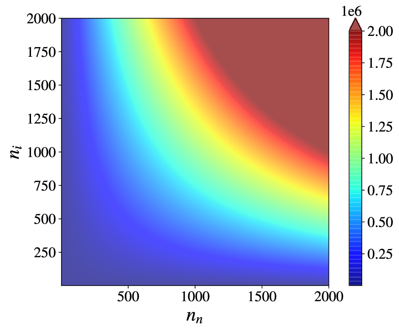
(a) Dense layer with parameters; number of features in the input vector $n_{i}$ and number of neurons in the layer $n_{n}$.

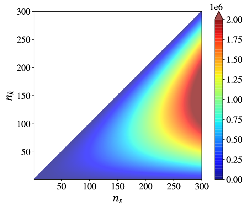
(b) CNN with parameters; kernel size $n_{k}$ and number of time steps $n_{s}$.

Figure 3: Number of real multiplications (RM) of feed-forward layers.

IV Comparative analysis of the complexities for each NN structure

The comparison of the complexity in terms of RM is illustrated in Fig. 3 for feed-forward NNs and in Fig. 4 for recurrent networks. In feed-forward networks, we first address the computational complexity for a dense layer. In order to reach over $2\times 10^{6}$ real multiplications, which we use as a threshold (highlighted by a maroon color), we can have up to around 1500 input features ($n_{i}$) and 1500 neurons ($n_{n}$) which is clearly a high value for a single dense layer. The $n_{n}n_{i}$ term in Eq. (3) forms a hyperbolic curve, as can be seen in Fig. 3(a). For the 1D-convolutional layer, as predicted by Eq. 11, we reach a high complexity (maroon) region using less input features than the dense layer case because now the complexity growth depends on more than 2 variables (e.g. to reach the complexity threshold, the number of time steps $n_{s}$ can be set to 275 with the kernel size $n_{k}$ equal to 150, and we fixed $n_{i}=100$, $n_{o}=1$, $padding=0$, $dilation=1$, and $stride=1$). According to the exemplary chosen parameters above, the $n_{k}\leq n_{s}$ condition derived from Eq. (10) must be satisfied in order to obtain at least the output size equal to 1; therefore, in Fig. 3(b), the white region corresponds to unavailable output and the heat-map has a hyperbolic form because only $n_{s}$ and $n_{k}$ parameters vary and the other parameters are kept constant.

The RNN-based networks apparently have higher complexity than the feed-forward NNs. The vanilla RNN in Fig. 4(a) shows the least complexity among the RNN-based networks studied, while the LSTM’s complexity growth is the fastest, which can be seen from the size of the maroon area in Fig. 4(b). The GRU in Fig. 4(c) shows slightly lower complexity than the LSTM because it has a lower number of gates in its architecture. If we look at the equations of GRU and LSTM in Table III, the LSTM has a multiplier of 4 for the $n_{i}$ and $n_{h}$, whereas for the GRU the multiplier is 3. The ESN with fixed $n_{o}=100$ and $s_{p}=0.5$ in Fig. 4(d) has higher complexity than the vanilla RNN, but less complexity than the GRU, because the ESN by design has a less complex architecture due to the use of the reservoir [64]. For all RNN-based networks, we readily infer that the number of hidden units $n_{h}$, or $N_{r}$ for the ESN, plays the most crucial role in defining the layer’s computational complexity in terms of RM metric. In Fig.4, we observe that the top face of all cubes which corresponds to the highest number of $n_{h}$ ($n_{h}=100$) has the largest maroon areas. In terms of the effect on the complexity behaviour, the second most important quantity is the number of time steps $n_{s}$; we can see in Fig. 4 that the right face of the cubes, referring to the highest number of $n_{s}$ ($n_{s}=100$), has the second-largest maroon areas. Finally, the dimensions of the input vector $n_{i}$ have the least impact on the RM, as shown by the left face ($n_{i}=100$) of all cubes in Fig. 4 with the smallest maroon areas compared to other faces. See Eqs. (3), (11), (15), (19), (23), and (29) for the exact dependencies.

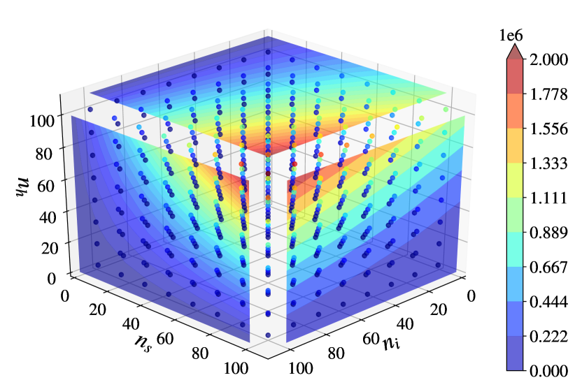
(a) Vanilla RNN.

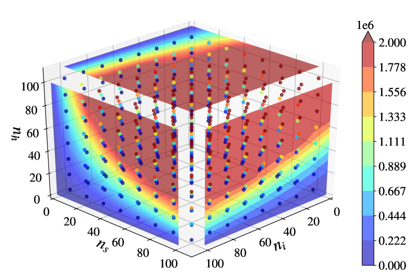
(b) LSTM.

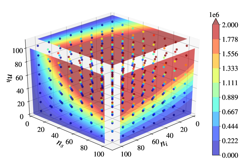
(c) GRU.

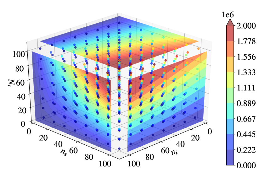
(d) ESN.

Figure 4: Number of real multiplications (RM) of recurrent layers with respect to different values of the number of features in the input vector $n_{i}$, the number of time steps $n_{s}$ and the number of hidden units $n_{h}$ or $N_{r}$ in ESN.

Furthermore, to highlight the computational complexity trend over those different recurrent layers, we plotted the RM versus the number of hidden units ($n_{h}$ for vanilla RNN, LSTM, and GRU, or $N_{r}$ in ESN) in a scenario where all other hyper-parameters are constant. Fig. 5(a) depicts the result of this analysis when $n_{s}=100$, $n_{i}=100$ for all networks, and $n_{o}=100$, $s_{p}=0.5$ for the ESN. By considering those parameters as fixed, the complexity of all four recurrent layers scales quadratically with the number of hidden units ($n_{h}^{2}$), which is traditionally interpreted as having the same $O(n^{2})$. However, Fig. 5(a) brings an important fact that there are significant differences in the computational complexity in terms of RM between all four recurrent layers. Ultimately, this means that the Big-$O$ notation is not sensitive enough to assess the complexity of the NNs in digital signal processing. We can spot that the LSTM complexity escalates the fastest followed by the GRU, ESN, and RNN, respectively. These differences result mainly from the scaling terms on the $n_{h}^{2}$ of each RM complexity expression for these layers. Note that for the ESN (Eq. (29)), the complexity increases more steadily, as far as, $N_{r}$ is multiplied to the sparsity parameter $s_{p}$. Moreover, as noted in Sec. III-F, the reservoir can be implemented in the optical domain, so the complexity can be reduced further at the expense of performance trade-off.

We notice that not only the hyper-parameters like $n_{h}$ and $n_{s}$, affect the computational complexity, but also the bitwidth or precision of each parameter can impact the complexity when we quantify it in terms of the BOP. The effects produced by bitwidth value of weight ($b_{w}$), input ($b_{i}$), and activation ($b_{a}$) are examined in this study. The full-precision or 32-bit precision can be considered over-redundant because 8-bit or less is often enough to provide comparable performance, as stated by many works in the field [65, 66, 67, 68]. Here, we did not provide the study of the BOP versus different hyper-parameters and bitwidth, because we believe that this is a straightforward analysis that approximately follows what we already studied with the RM metric. Instead, we focus on answering the following question: which variable bitwidth ($b_{w}$, $b_{i}$, or $b_{a}$) produces the highest saving in the BOP complexity when its precision is reduced?. This question can guide the design of a low complexity NN structure by identifying which parameter of the NN is the key to producing the higher saving in complexity. To address this question, we compare the reduction of the BOP when using 8-bit precision versus the 4-bit precision for each parameter ($b_{w}$, $b_{i}$, and $b_{a}$) in different network types; the results of the comparison are shown in Fig. 5(b). The bitwidth of the weight matrix $b_{w}$ is the most significant parameter to consider when trying to reduce the layer’s complexity, as the BOP is decreased by around 40% for all network types when we halved the precision of $b_{w}$. For the dense and 1D-convolutional layers, the precision for input $b_{i}$ is as important as the $b_{w}$, while reducing the bitwidth of the bias vector $b_{a}$ does not have a noticeable impact on the BOP. In the RNN-based networks, converting from 8-bit to 4-bit precision for $b_{i}$ and $b_{a}$ shows a nearly equivalent reduction in the BOP, except for the ESN case, where decreasing the $b_{a}$ precision results in more reduction in the BOP than when we reduce the $b_{i}$ precision.

Lastly, we analyze the NABS metric considering various quantization techniques: uniform, PoT and APoT quantization, as described in Sec. III-A. Note that each technique needs a different number of shifts and adders to perform the multiplication. As mentioned before, the shifts incur no extra cost in hardware implementation; therefore, we focus on evaluating the NABS metric of each layer for certain quantization techniques versus the number of adders required at most to perform the multiplication, denoting it as $X$. More specifically, if the weight matrix has $b_{w}$ as its bitwidth and the uniform quantization is utilized, the number of adders required at most ($X_{w}$) is equal $b_{w}-1$. In the case of PoT, $X_{w}=0$, and for APoT, $X_{w}$ varies between 1 and $b_{w}-2$, in this case. Fig. 5(c) shows the NABS versus $X_{w}$ analysis when considering that: $b_{w},b_{i},b_{a}=8$ for all networks, $n_{i}=1000$ and $n_{n}=2000$ for a dense layer, $n_{i}=100$, $n_{s}=300$, $n_{o}=1$, $padding=0$, $dilation=1$, $stride=1$ and $n_{k}=100$ for a 1D-convolutional layer, $n_{i}=100$, $n_{s}=100$ and $n_{h}=100$ for all RNN-based networks, and $n_{o}=100$, $s_{p}=0.5$ for the ESN.

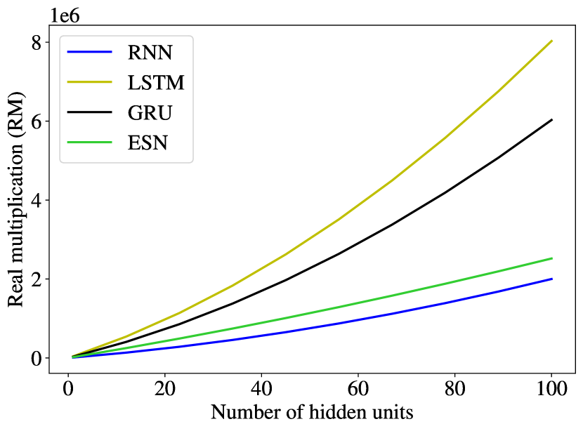
(a)

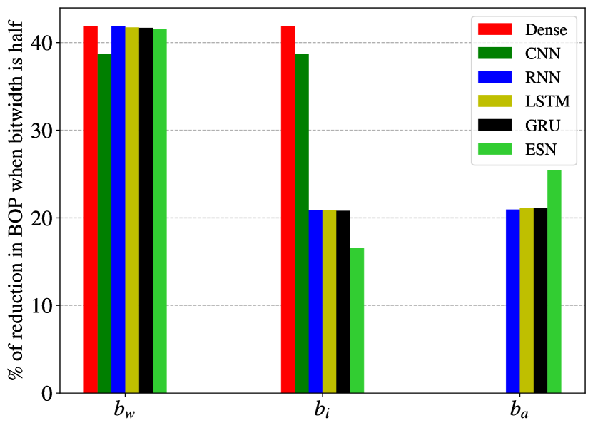
(b)

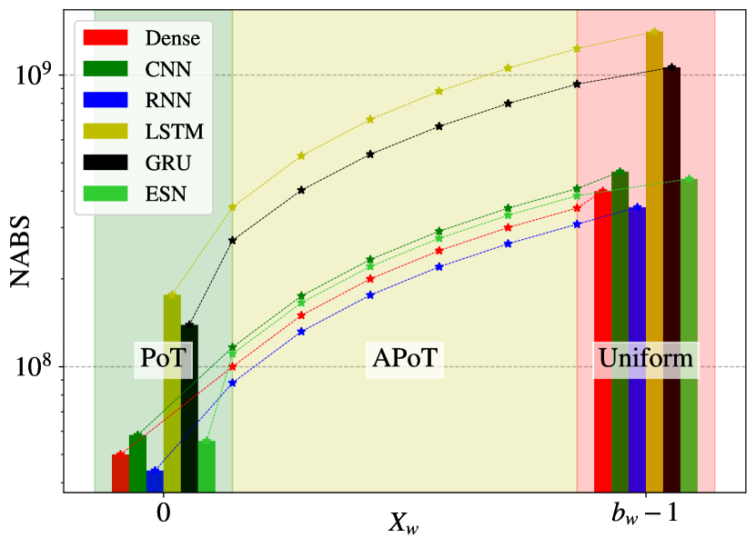
(c)

Figure 5: (a) Complexity comparison between recurrent-based networks when $n_{s}$ = 100, $n_{i}$ = 100 for all networks and $n_{o}$ = 100, $s_{p}$ = 0.5 for ESN; (b) Reduction of BOP in percentage when reducing bitwidth of each parameter; weight bidtwidth $b_{w}$, input bidtwidth $b_{i}$, and activation bidtwidth $b_{a}$ by half or from 8 bits to 4 bits; (c) Comparison of the number of additions and bit shifts (NABS) with different quantization techniques and different network types, assume $b_{w}=8$. Note that $X_{w}$ is the number of adders required to represent a multiplier.

As it is shown in Fig. 5(c), for all types of networks, when the PoT quantization is used, the NABS can drop around 8 times lower compared to the NABS when using the uniform quantization. Since APoT is a quantization scheme represented by a sum of PoT terms, APoT provides a smooth transition between PoT and uniform quantization. In various works, PoT was claimed to have very low complexity because the multiplications are replaced by just shifts [69, 70, 53]. However, when we consider that the multiplication in the uniform quantization can be represented by shifts and adders, and we have a fair metric like NABS to compare between different quantization techniques, the NABS when applying PoT is only around an order of magnitude lower than the NABS when using the uniform quantization. To be more specific, even though PoT converts all multipliers into bit shifters, we still have a number of adders coming from the sum operations which are not related to the multipliers, but are they are key for the operational structure of the NN layers. Therefore, the NABS metric can provide a reliable assessment of the computational complexity of NNs before their implementation in hardware, where the NLG will be the ultimate metric. Note that we intentionally increased the values of the hyper-parameters for the feed-forward NNs in order to compare them in the same graph as the RNN-based networks. For the complexity with regard to NABS, the LSTM apparently needs the highest number of shifts and adders. In conclusion, the three matrices of complexity: the RM, the BOP, and the NABS, have the same trend, meaning that the LSTM requires the most computational resources, followed by the GRU. However, the complexity depends on the particular NN design and can be reduced if we can tolerate a more accurate trade-off: varying the values of hyper-parameters can affect the accuracy, but, simultaneously, work in favour to reduce the computational complexity.

V Conclusion

In this work, we described the systematic approach for how to evaluate the computational complexity in terms of the three metrics (noticing that the fourth one, the number of logic gates, is hardware dependent and cannot be calculated without referring to a particular setup): the number of real multiplications (RM), the number of bit operations (BOP), and the number of additions and bit shifts (NABS); this itemization implies that we are gradually changing from the software to hardware level. The introduction of such detailed metrics has offered us an opportunity to establish a baseline for the complexity calculation in a more consistent way, depending on the purpose. We investigated the computation of RM, BOP, and NABS in feed-forward and recurrent layers, addressing, namely, a dense layer, a 1D-convolutional layer, a vanilla RNN, LSTM, GRU, and ESN architectures in rather general form.

First, we evaluated the RM metric showing how complexity evolves when changing different hyper-parameters of each NN layer. Specifically, for the recurrent layers, as it was actually expected, the LSTM has the highest complexity among the examined NNs, because of RNN’s architecture featuring different types of gates; moreover, the LSTM complexity grows dramatically with the rise of the number of hidden units. The least complex recurrent architecture is the vanilla RNN. For all recurrent networks, the most complexity-impactful hyper-parameter is the number of hidden units, followed by the number of time steps; the size of the input vector is the least influential. Here, we note that the dense layer is the NN layer type that is the cheapest in terms of complexity, because it is just a matrix multiplication, while all other layers imply a more complex processing procedure.

Our paper also shows the importance of bitwidth (or the precision) for defining the complexity expressed in terms of BOP, i.e. when we descend closer to the hardware level. With the two times reduction in bitwidth, especially in the bitwidth of the weights, the BOP gets drastically reduced, becoming around 40% lower for all types of NNs. This fact shows that when designing the NN solutions, we should prioritize low precision bit in the NN weights to achieve a better reduction in complexity.

Finally, this paper introduces the new metric named NABS to highlight the effects of different quantization techniques: uniform, PoT, and APoT. Different from the other papers claiming that the complexity can be reduced drastically when applying the PoT, our current work shows that by using a fair complexity metric like the NABS, the true complexity (i.e. the NABS metric) gets reduced by only around one order of magnitude when using the PoT compared to the uniform quantization for all NN layers. Thus, we claim that the new metric NABS identifies the true complexity level (or the reduction level) better than the previously used RM or BOP.

References

- [1] A. Miller, B. Blott et al., “Review of neural network applications in medical imaging and signal processing,” Medical and Biological Engineering and Computing, vol. 30, no. 5, pp. 449–464, 1992.
- [2] L. A. Feldkamp and G. V. Puskorius, “A signal processing framework based on dynamic neural networks with application to problems in adaptation, filtering, and classification,” Proceedings of the IEEE, vol. 86, no. 11, pp. 2259–2277, 1998.
- [3] S. Kiranyaz, O. Avci, O. Abdeljaber, T. Ince, M. Gabbouj, and D. J. Inman, “1d convolutional neural networks and applications: A survey,” Mechanical systems and signal processing, vol. 151, p. 107398, 2021.
- [4] H. Dahrouj, R. Alghamdi, H. Alwazani, S. Bahanshal, A. A. Ahmad, A. Faisal, R. Shalabi, R. Alhadrami, A. Subasi, M. T. Al-Nory, O. Kittaneh, and J. S. Shamma, “An overview of machine learning-based techniques for solving optimization problems in communications and signal processing,” IEEE Access, vol. 9, pp. 74 908–74 938, 2021.
- [5] S.-i. Amari and A. Cichocki, “Adaptive blind signal processing-neural network approaches,” Proceedings of the IEEE, vol. 86, no. 10, pp. 2026–2048, 1998.
- [6] K. Burse, R. N. Yadav, and S. Shrivastava, “Channel equalization using neural networks: A review,” IEEE Transactions on Systems, Man, and Cybernetics, Part C (Applications and Reviews), vol. 40, no. 3, pp. 352–357, 2010.
- [7] M. Kahrs and K. Brandenburg, Applications of digital signal processing to audio and acoustics. Springer Science & Business Media, 1998.
- [8] R. Govil, “Neural networks in signal processing,” Fuzzy Systems and Soft Computing in Nuclear Engineering, pp. 235–257, 2000.
- [9] B. Lusch, J. N. Kutz, and S. L. Brunton, “Deep learning for universal linear embeddings of nonlinear dynamics,” Nature Communications, vol. 9, no. 1, pp. 1–10, 2018.
- [10] H. Huttunen, “Deep neural networks: A signal processing perspective,” in Handbook of signal processing systems. Springer, 2019, pp. 133–163.
- [11] M. A. Jarajreh, E. Giacoumidis, I. Aldaya, S. T. Le, A. Tsokanos, Z. Ghassemlooy, and N. J. Doran, “Artificial neural network nonlinear equalizer for coherent optical ofdm,” IEEE Photonics Technology Letters, vol. 27, no. 4, pp. 387–390, 2015.
- [12] F.-L. Luo and R. Unbehauen, Applied neural networks for signal processing. Cambridge university press, 1998.
- [13] M. Ibnkahla, “Applications of neural networks to digital communications–a survey,” Signal processing, vol. 80, no. 7, pp. 1185–1215, 2000.
- [14] D. Malkoff, “A neural network for real-time signal processing,” Advances in Neural Information Processing Systems, vol. 2, 1989.
- [15] V. Sze, Y.-H. Chen, T.-J. Yang, and J. S. Emer, “Efficient processing of deep neural networks: A tutorial and survey,” Proceedings of the IEEE, vol. 105, no. 12, pp. 2295–2329, 2017.
- [16] P. Gysel, M. Motamedi, and S. Ghiasi, “Hardware-oriented approximation of convolutional neural networks,” arXiv preprint arXiv:1604.03168, 2016.
- [17] B. Li and T. N. Sainath, “Reducing the computational complexity of two-dimensional lstms.” in INTERSPEECH, 2017, pp. 964–968.
- [18] T.-J. Yang, Y.-H. Chen, and V. Sze, “Designing energy-efficient convolutional neural networks using energy-aware pruning,” in Proceedings of the IEEE conference on computer vision and pattern recognition, 2017, pp. 5687–5695.
- [19] J. L. Balcázar, R. Gavalda, and H. T. Siegelmann, “Computational power of neural networks: A characterization in terms of kolmogorov complexity,” IEEE Transactions on Information Theory, vol. 43, no. 4, pp. 1175–1183, 1997.
- [20] M. Van Baalen, C. Louizos, M. Nagel, R. A. Amjad, Y. Wang, T. Blankevoort, and M. Welling, “Bayesian bits: Unifying quantization and pruning,” Advances in neural information processing systems, vol. 33, pp. 5741–5752, 2020.
- [21] C. Baskin, N. Liss, E. Schwartz, E. Zheltonozhskii, R. Giryes, A. M. Bronstein, and A. Mendelson, “Uniq: Uniform noise injection for non-uniform quantization of neural networks,” ACM Transactions on Computer Systems (TOCS), vol. 37, no. 1-4, pp. 1–15, 2021.
- [22] S. Deligiannidis, C. Mesaritakis, and A. Bogris, “Performance and complexity analysis of bi-directional recurrent neural network models versus volterra nonlinear equalizers in digital coherent systems,” Journal of Lightwave Technology, vol. 39, no. 18, pp. 5791–5798, 2021.
- [23] O. Sidelnikov, A. Redyuk, and S. Sygletos, “Equalization performance and complexity analysis of dynamic deep neural networks in long haul transmission systems,” Optics Express, vol. 26, no. 25, pp. 32 765–32 776, 2018.
- [24] P. J. Freire, Y. Osadchuk, B. Spinnler, A. Napoli, W. Schairer, N. Costa, J. E. Prilepsky, and S. K. Turitsyn, “Performance versus complexity study of neural network equalizers in coherent optical systems,” Journal of Lightwave Technology, vol. 39, no. 19, pp. 6085–6096, 2021.
- [25] W. Maass, “On the computational complexity of networks of spiking neurons,” Advances in neural information processing systems, vol. 7, 1994.
- [26] R. Alizadeh, J. K. Allen, and F. Mistree, “Managing computational complexity using surrogate models: a critical review,” Research in Engineering Design, vol. 31, no. 3, pp. 275–298, 2020.
- [27] S. Wiedemann, K.-R. Müller, and W. Samek, “Compact and computationally efficient representation of deep neural networks,” IEEE transactions on neural networks and learning systems, vol. 31, no. 3, pp. 772–785, 2019.
- [28] A. M. Amin, R. R. Mahmood, and A. I. Khan, “Analysis of pattern recognition algorithms using associative memory approach: a comparative study between the hopfield network and distributed hierarchical graph neuron (dhgn),” in 2008 IEEE 8th International Conference on Computer and Information Technology Workshops. IEEE, 2008, pp. 153–158.
- [29] S. N. Kerr, “A big-o experiment: which function is it?” in Proceedings of the 43rd annual Southeast regional conference-Volume 1, 2005, pp. 317–318.
- [30] V. D. Blondel and J. N. Tsitsiklis, “A survey of computational complexity results in systems and control,” Automatica, vol. 36, no. 9, pp. 1249–1274, 2000.
- [31] E. Jacobsen and P. Kootsookos, “Fast, accurate frequency estimators [dsp tips & tricks],” IEEE Signal Processing Magazine, vol. 24, no. 3, pp. 123–125, 2007.
- [32] B. Spinnler, “Equalizer design and complexity for digital coherent receivers,” IEEE Journal of Selected Topics in Quantum Electronics, vol. 16, no. 5, pp. 1180–1192, 2010.
- [33] S. Mirzaei, A. Hosangadi, and R. Kastner, “Fpga implementation of high speed fir filters using add and shift method,” in 2006 International Conference on Computer Design. IEEE, 2006, pp. 308–313.
- [34] S. Jahani, “Zot-mk: a new algorithm for big integer multiplication,” MSc MSc, Department of Computer Science, Universiti Sains Malaysia, Penang, 2009.
- [35] B. Hawks, J. Duarte, N. J. Fraser, A. Pappalardo, N. Tran, and Y. Umuroglu, “Ps and qs: Quantization-aware pruning for efficient low latency neural network inference,” arXiv preprint arXiv:2102.11289, 2021.
- [36] J. Wu, Y. Wang, Z. Wu, Z. Wang, A. Veeraraghavan, and Y. Lin, “Deep k-means: Re-training and parameter sharing with harder cluster assignments for compressing deep convolutions,” in International Conference on Machine Learning. PMLR, 2018, pp. 5363–5372.
- [37] X. Staff, “Gate count capacity metrics for fpgas,” Xilinx Corp., San Jose, CA, Application Note XAPP, vol. 59, 1997.
- [38] Y. Li, X. Dong, and W. Wang, “Additive powers-of-two quantization: An efficient non-uniform discretization for neural networks,” arXiv preprint arXiv:1909.13144, 2019.
- [39] T. Koike-Akino, Y. Wang, K. Kojima, K. Parsons, and T. Yoshida, “Zero-multiplier sparse dnn equalization for fiber-optic qam systems with probabilistic amplitude shaping,” in 2021 European Conference on Optical Communications (ECOC). IEEE, 2021, pp. 1–4.
- [40] M. Elhoushi, Z. Chen, F. Shafiq, Y. H. Tian, and J. Y. Li, “Deepshift: Towards multiplication-less neural networks,” in Proceedings of the IEEE/CVF Conference on Computer Vision and Pattern Recognition, 2021, pp. 2359–2368.
- [41] H. You, X. Chen, Y. Zhang, C. Li, S. Li, Z. Liu, Z. Wang, and Y. Lin, “Shiftaddnet: A hardware-inspired deep network,” arXiv preprint arXiv:2010.12785, 2020.
- [42] P. Gentili, F. Piazza, and A. Uncini, “Efficient genetic algorithm design for power-of-two fir filters,” in 1995 International conference on acoustics, speech, and signal processing, vol. 2. IEEE, 1995, pp. 1268–1271.
- [43] J. B. Evans, “Efficient fir filter architectures suitable for fpga implementation,” IEEE Transactions on Circuits and Systems II: Analog and Digital Signal Processing, vol. 41, no. 7, pp. 490–493, 1994.
- [44] W. R. Lee, V. Rehbock, K. L. Teo, and L. Caccetta, “Frequency-response masking based fir filter design with power-of-two coefficients and suboptimum pwr,” Journal of Circuits, Systems, and Computers, vol. 12, no. 05, pp. 591–599, 2003.
- [45] P. Kurup and T. Abbasi, Logic synthesis using Synopsys®. Springer Science & Business Media, 2012.
- [46] H. Li and W. Ye, “Efficient implementation of fpga based on vivado high level synthesis,” in 2016 2nd IEEE International Conference on Computer and Communications (ICCC), 2016, pp. 2810–2813.
- [47] X. Inc., “Ultrascale architecture dsp slice,” 2021. [Online]. Available: https://docs.xilinx.com/v/u/en-US/ug579-ultrascale-dsp
- [48] N. Tran, B. Hawks, J. M. Duarte, N. J. Fraser, A. Pappalardo, and Y. Umuroglu, “Ps and qs: Quantization-aware pruning for efficient low latency neural network inference,” Frontiers in Artificial Intelligence, vol. 4, p. 94, 2021.
- [49] S. V. Padmajarani and M. Muralidhar, “Fpga implementation of multiplier using shift and add technique,” International Journal of Advances in Electronics and Computer Science-IJAECS, vol. 2, no. 9, pp. 1–5, 2015.
- [50] V. S. Dimitrov, K. U. Jarvinen, and J. Adikari, “Area-efficient multipliers based on multiple-radix representations,” IEEE Transactions on Computers, vol. 60, no. 2, pp. 189–201, 2010.
- [51] R. I. Hartley, “Subexpression sharing in filters using canonic signed digit multipliers,” IEEE Transactions on Circuits and Systems II: Analog and Digital Signal Processing, vol. 43, no. 10, pp. 677–688, 1996.
- [52] V. Dimitrov, L. Imbert, and A. Zakaluzny, “Multiplication by a constant is sublinear,” in 18th IEEE Symposium on Computer Arithmetic (ARITH’07). IEEE, 2007, pp. 261–268.
- [53] D. Przewlocka-Rus, S. S. Sarwar, H. E. Sumbul, Y. Li, and B. De Salvo, “Power-of-two quantization for low bitwidth and hardware compliant neural networks,” arXiv preprint arXiv:2203.05025, 2022.
- [54] Y. Bengio, P. Simard, and P. Frasconi, “Learning long-term dependencies with gradient descent is difficult,” IEEE Transactions on Neural Networks, vol. 5, no. 2, pp. 157–166, 1994.
- [55] Z. C. Lipton, J. Berkowitz, and C. Elkan, “A critical review of recurrent neural networks for sequence learning,” arXiv preprint arXiv:1506.00019, 2015.
- [56] S. Hochreiter and J. Schmidhuber, “Long short-term memory,” Neural computation, vol. 9, no. 8, pp. 1735–1780, 1997.
- [57] F. A. Gers, J. Schmidhuber, and F. Cummins, “Learning to forget: Continual prediction with lstm,” Neural computation, vol. 12, no. 10, pp. 2451–2471, 2000.
- [58] R. Dey and F. M. Salem, “Gate-variants of gated recurrent unit (gru) neural networks,” in 2017 IEEE 60th international midwest symposium on circuits and systems (MWSCAS). IEEE, 2017, pp. 1597–1600.
- [59] Q. Wu, E. Fokoue, and D. Kudithipudi, “On the statistical challenges of echo state networks and some potential remedies,” arXiv preprint arXiv:1802.07369, 2018.
- [60] M. Sorokina, S. Sergeyev, and S. Turitsyn, “Fiber echo state network analogue for high-bandwidth dual-quadrature signal processing,” Optics express, vol. 27, no. 3, pp. 2387–2395, 2019.
- [61] S. S. Mosleh, L. Liu, C. Sahin, Y. R. Zheng, and Y. Yi, “Brain-inspired wireless communications: Where reservoir computing meets mimo-ofdm,” IEEE Transactions on Neural Networks and Learning Systems, vol. 29, no. 10, pp. 4694–4708, 2018.
- [62] C. Sun, M. Song, S. Hong, and H. Li, “A review of designs and applications of echo state networks,” arXiv preprint arXiv:2012.02974, 2020.
- [63] H. Jaeger, M. Lukoševičius, D. Popovici, and U. Siewert, “Optimization and applications of echo state networks with leaky-integrator neurons,” Neural networks, vol. 20, no. 3, pp. 335–352, 2007.
- [64] E. López, C. Valle, H. Allende-Cid, and H. Allende, “Comparison of recurrent neural networks for wind power forecasting,” in Mexican Conference on Pattern Recognition. Springer, 2020, pp. 25–34.
- [65] H. Yu, H. Li, H. Shi, T. S. Huang, G. Hua et al., “Any-precision deep neural networks,” arXiv preprint arXiv:1911.07346, vol. 1, 2019.
- [66] R. Banner, I. Hubara, E. Hoffer, and D. Soudry, “Scalable methods for 8-bit training of neural networks,” Advances in neural information processing systems, vol. 31, 2018.
- [67] K. Wang, Z. Liu, Y. Lin, J. Lin, and S. Han, “Haq: Hardware-aware automated quantization with mixed precision,” in Proceedings of the IEEE/CVF Conference on Computer Vision and Pattern Recognition, 2019, pp. 8612–8620.
- [68] I. Hubara, Y. Nahshan, Y. Hanani, R. Banner, and D. Soudry, “Accurate post training quantization with small calibration sets,” in International Conference on Machine Learning. PMLR, 2021, pp. 4466–4475.
- [69] M. Marchesi, G. Orlandi, F. Piazza, and A. Uncini, “Fast neural networks without multipliers,” IEEE transactions on Neural Networks, vol. 4, no. 1, pp. 53–62, 1993.
- [70] S.-E. Chang, Y. Li, M. Sun, W. Jiang, R. Shi, X. Lin, and Y. Wang, “Msp: an fpga-specific mixed-scheme, multi-precision deep neural network quantization framework,” arXiv preprint arXiv:2009.07460, 2020.