Towards a consistent model of the hot quadruple system HD 93206 = QZ Carinæ: II. N-body model

Abstract

Aims. HD 93206 is early-type massive stellar system, composed of components resolved by direct imaging (Ab, Ad, B, C, D) as well as a compact sub-system (Aa1, Aa2, Ac1, Ac2). Its geometry was already determined on the basis of extensive photometric, spectroscopic and interferometric observations. However, the fundamental absolute parameters are still not known precisely enough.

Methods. We use an advanced N-body model to account for all mutual gravitational perturbations among the four close components, and all observational data types, including: astrometry, radial velocities, eclipse timing variations, squared visibilities, closure phases, triple products, normalized spectra, and spectral-energy distribution (SED). The respective model has 38 free parameters, namely three sets of orbital elements, component masses, and their basic radiative properties ($T$, $\log g$, $v_{\rm rot}$).

Results. We revised the fundamental parameters of QZ Car as follows. For a model with the nominal extinction coefficient $R_{V}\equiv A_{V}/E(B-V)=3.1$, the best-fit masses are $m_{1}=26.1\,M_{\rm S}$, $m_{2}=32.3\,M_{\rm S}$, $m_{3}=70.3\,M_{\rm S}$, $m_{4}=8.8\,M_{\rm S}$, with uncertainties of the order of $2\,M_{\rm S}$, and the system distance $d=(2800\pm 100)\,{\rm pc}$. In an alternative model, where we increased the weights of RV and TTV observations and relaxed the SED constraints, because extinction can be anomalous with $R_{V}\sim 3.4$, the distance is smaller, $d=(2450\pm 100)\,{\rm pc}$. This would correspond to that of Collinder 228 cluster. Independently, this is confirmed by dereddening of the SED, which is only then consistent with the early-type classification (O9.7Ib for Aa1, O8III for Ac1). Future modelling should also account for an accretion disk around Ac2 component.

1 Introduction

HD 93206 is a complex system composed of nine components (usually denoted as Aa1, Aa2, Ac1, Ac2, Ab, Ad, B, C, D; Mason et al. 2001). In the accompanying paper Mayer et al. (2022), we used several observation-specific models to obtain fundamental parameters of its sub-systems, in particular the eclipsing binary Ac1+Ac2, the spectroscopic binary Aa1+Aa2, and their mutual long-period orbit (Aa1+Aa2)+(Ac1+Ac2). Together, the quadruple sub-system is denoted as QZ Car variable star. All these models were kinematical, i.e., based the two-body problem with the light-time effect and the third light, to account at least for major perturbations.

In this work, we focus on the same quadruple sub-system QZ Car, but we use a dynamical N-body model called Xitau, to account for additional perturbations (in particular, all mutual, parametrized post-Newtonian). Moreover, we account for all observational datasets at the same time, including astrometry, photometry, spectroscopy, interferometry, etc. This approach allows us to derive robust estimates of fundamental parameters. Our model was already used for multiple stellar systems (e.g, $\xi$ Tau, Nemravová et al. 2016; Brož 2017) and asteroidal moons systems with highly-irregular central bodies (e.g., (216), Marchis et al. 2021; Brož et al. 2021a, 2022).

2 Observational datasets

While radial velocity measurements, relative spectroscopy, light curves and corresponding eclipse-timing variations (ETVs), and astrometry were already described in Mayer et al. (2022), here we focus on additional datasets, namely the spectral-energy distribution and interferometry.

2.1 Spectral-energy distribution (SED)

We used data from Vizier, which included the standard Johnson system photometry (Ducati, 2002), verified by La Silla and Sutherland photometry (see Mayer et al. 2022), Hipparcos (Anderson & Francis, 2012), GAIA3 (Gaia Collaboration, 2020), 2MASS (Cutri et al., 2003), WISE (Cutri & et al., 2012), MSX (Egan et al., 2003), and Akari (Ishihara et al., 2010). Altogether, the whole spectral range is $0.35$ to $22\,\mu{\rm m}$.

It was necessary to carry out dereddening of these data. Unfortunately, classic extinction maps of Green et al. (2019) give unrealistic absorption and a special treatment is needed for QZ Car, which is too close to the galactic equator. To this point, we used extinction maps of Lallement et al. (2019). For the assumed distance 2870 pc (Shull & Danforth, 2019), the reddening extrapolated from 2100 pc is $E(B-V)=(0.470\pm 0.060)\,{\rm mag}$, and corresponding absorption $A_{V}=3.1\,E(B-V)=(1.46\pm 0.19)\,{\rm mag}$ (Fig. 1). Using the standard wavelength dependence of Schlafly & Finkbeiner (2011), we obtained the dereddened fluxes, shown in Fig. 2.

Not surprisingly, the corrected fluxes exhibit a power-law slope, which corresponds to the Planck function ($B_{\lambda}\propto\lambda^{-4}$ for $\lambda>0.35\,\mu{\rm m}$), for the effective temperature $T\simeq 30000\,{\rm K}$. This is in agreement with the early-type spectral classification of QZ Car. Using a significantly smaller distance (e.g., 2000 pc) would result in a SED which does not correspond to early-type stars. We shall see later in Section 3 that this distance and dereddening are indeed reliable. On the other hand, in far infrared (${>}\,2.2\,\mu{\rm m}$), where absorption is already negligible, a non-negligible excess is present. The monochromatic fluxes are a factor of 5 too large, possibly indicating cold circumstellar matter or blending, neither of which is accounted for in our modelling. Consequently, we should preferably fit the NUV–NIR spectral range.

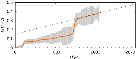
Figure 1: Reddening $E(B-V)$ vs. distance for the direction towards QZ Car, according to Lallement et al. (2019). The mean (orange), dispersion (gray), and extrapolation (dashed) to the nominal distance 2870 pc are shown.

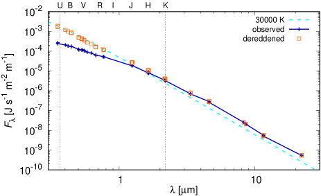
Figure 2: Observed spectral-energy distribution (SED; blue) and dereddened SED (orange) for the distance 2870 pc. The dereddened fluxes $F_{\lambda}$ approximately correspond to black-body radiation with the temperature 30 000 K (cyan). In far infrared, where absorption is negligible, a non-negligible (half order) excess is present.

2.2 Interferometry

Additionally to Sanchez-Bermudez et al. (2017) astrometric data, for the epochs Jun 17th 2016, Jun 18th 2016, we used interferometric observations with the VLTI/GRAVITY instrument, found in the ESO archive for the epochs Mar 14th 2017, Apr 27th 2017. This is an important constraint for the (Ac1+Ac2)+(Aa1+Aa2) orbit. Apart from astrometry, we can directly include squared visibilities $V^{2}$, closure phases ${\rm arg}T_{3}$, and triple product amplitudes $|T_{3}|$ in Xitau.

We used the Esoreflex VLTI/GRAVITY pipeline (Freudling et al., 2013; Gravity Collaboration et al., 2017) to reduce the data. We performed the standard visibility calibration, which is substantial (0.2) for baselines $\geq 4.5\times 10^{7}$ cycles per baseline. We used the so-called ‘vfactor’ for the correction of $V^{2}$. We did not use data with $V^{2}+\sigma_{V^{2}}>1.0$. The new $(u,v)$ coverage is shown in Fig. 3. The wide orbit ((Ac1+Ac2)+(Aa1+Aa2)), having the angular separation more than $30\,{\rm mas}$, is clearly resolved. On the other hand, angular diameters of individual components ($0.015$ to $0.08\,{\rm mas}$) cannot be resolved. We shall see later in Section 3, there were some problems with $|T_{3}|$ calibration. Consequently, we also tried to reduce the data without ‘vfactor’.

As a check, we performed astrometry with the Litpro software (Tallon-Bosc et al., 2008). A simplified model of a binary (Ac+Aa) was assumed. We fitted $(u,v)$ coordinates of Aa and the flux ratio $F_{\rm Aa}/F_{\rm Ac}$; other parameters were kept fixed. Even though there are some systematics, the fit converges without problems and astrometric uncertainties are comparable to previous measurements ($\sigma_{u,v}\simeq 0.010\,{\rm mas}$; Tab. 1).

We used no light curves in our modelling (only indirectly as ETVs). To our knowledge, there are no sufficiently high-signal-to-noise differential interferometric measurements (cf. Sanchez-Bermudez et al. (2017)), which would otherwise constrain velocity-dependent visibilities across spectral lines.

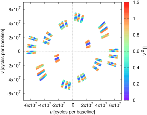
Figure 3: Coverage $(u,v)\equiv\@vec{B}/\lambda$ (in cycles per baseline) of new interferometric observations (see Tab. 1). The corresponding squared visibility $V^{2}$ is plotted in colour. The wide orbit ((Ac1+Ac2)+(Aa1+Aa2)), having the angular separation more than $30\,{\rm mas}$, is clearly resolved.

Table 1: Astrometric positions of component (Ac1+Ac2) with respect to (Aa1+Aa2) from literature and new data.

time	$u$	$v$	major	minor	P.A.	$F_{\rm Ac}/F_{\rm Aa}$	Ref.
(UTC)	mas	mas	mas	mas	deg	1
2012.1241	13.590	24.538	5.410	4.705	331.020	$0.68\pm 0.10$	Sana et al. (2014)
2012.4409	12.367	22.597	0.540	0.652	331.310	$0.37\pm 0.04$	Sana et al. (2014)
2016-06-18T01:35:21	15.940	25.609	0.045	0.054	0	$0.74\pm 0.14$	Sanchez-Bermudez et al. (2017)
2017-03-14T03:34:17	16.370	25.672	0.003	0.003	0	$0.490\pm 0.001$	ESO archive 098.D-0706(B)
2017-04-27T01:20:12	16.390	25.664	0.003	0.003	0	$0.571\pm 0.001$	ESO archive 099.D-0777(B)
2017-04-27T02:08:58	16.402	25.678	0.003	0.003	0	$0.573\pm 0.001$	ESO archive 099.D-0777(B)

3 Dynamical N-body model

In Xitau, the dynamical model contains the following accelerations terms (Brož, 2017; Brož et al., 2021a, 2022):

$$\@vec{f}=-\sum_{j\neq i}^{N}{Gm_{j}\over r_{ij}^{3}}\@vec{r}_{ij}+\@vec{f}_{\rm ppn}+\@vec{f}_{\rm oblat}+\@vec{f}_{\rm multipole}+\@vec{f}_{\rm tides}\,,$$ (1)

where the terms are mutual gravitational interactions and the parametrized post-Newtonian (PPN); we do not activate oblateness, multipoles or tides for QZ Car. We superseded the PPN approximation by that of Standish & Williams (2006), which is more accurate. Hereinafter, the notation conforms to the actual implementation:

$$\@vec{f}_{\rm ppn} = \sum_{j\neq i}^{N}\,\bigl{[}-K_{1}\left(K_{2}+K_{3}+K_{4}+K_{5}+K_{6}+K_{7}+K_{8}\right)\@vec{r}_{ij}+$$ (3)

$$+\,K_{1}\left(K_{9}+K_{10}\right)\dot{\@vec{r}}_{ij}+K_{11}\ddot{\@vec{r}}_{j}\bigr{]}\,,$$

$$K_{1}={1\over c^{2}}{Gm_{j}\over r_{ij}^{3}}\,,$$ (4)

$$K_{2}=-2(\beta+\gamma)\sum_{k\neq i}{Gm_{k}\over r_{ik}}\,,$$ (5)

$$K_{3}=-(2\beta-1)\sum_{k\neq j}{Gm_{k}\over r_{jk}}\,,$$ (6)

$$K_{4}=\gamma v_{i}^{2}\,,$$ (7)

$$K_{5}=(1+\gamma)v_{j}^{2}\,,$$ (8)

$$K_{6}=-2(1+\gamma)\,\dot{\@vec{r}}_{i}\!\cdot\dot{\@vec{r}}_{j}\,,$$ (9)

$$K_{7}=-{3\over 2}{(\@vec{r}_{ij}\cdot\dot{\@vec{r}}_{j})^{2}\over r_{ij}^{2}}\,,$$ (10)

$$K_{8}={1\over 2}\@vec{r}_{ji}\cdot\ddot{\@vec{r}}_{j}\,,$$ (11)

$$K_{9}=(2+2\gamma)\,\@vec{r}_{ij}\!\cdot\dot{\@vec{r}}_{i}\,,$$ (12)

$$K_{10}=-(1+2\gamma)\,\@vec{r}_{ij}\!\cdot\dot{\@vec{r}}_{j}\,,$$ (13)

$$K_{11}={3+4\gamma\over 2c^{2}}{Gm_{j}\over r_{ij}}\,,$$ (14)

where $\@vec{r}_{i}$ denotes the position vector of body $i$, $\@vec{r}_{ij}\equiv\@vec{r}_{i}-\@vec{r}_{j}$, $v_{i}\equiv|\dot{\@vec{r}}_{i}|$, $c$ the speed of light in vacuum, and $\beta=\gamma=1$ the nominal PPN factors.

We perform a numerical integration of orbits with the Bulirsch-Stoer algorithm. It has an adaptive time step, with the relative precision set to $10^{-8}$. The output time step is set to $0.2\,{\rm d}$, but all times of observations are also integrated and output precisely. The total number of free parameters is 38 (see Tab. 2). Observables are derived from coordinates, velocities, radiative quantities, and distance. Synthetic spectra, both relative and absolute, are computed during convergence with Pyterpol (Nemravová et al., 2016) from BSTAR, OSTAR grids (Lanz & Hubeny, 2007, 2003).

Observations and our model are compared by means of the $\chi^{2}$ metric:

$$\chi^{2} = w_{\rm rv}\chi^{2}_{\rm rv}+w_{\rm ttv}\chi^{2}_{\rm ttv}+w_{\rm vis}\chi^{2}_{\rm vis}+w_{\rm clo}\chi^{2}_{\rm clo}+w_{\rm t3}\chi^{2}_{\rm t3}\,+$$ (15)

$$+\,w_{\rm syn}\chi^{2}_{\rm syn}+w_{\rm sed}\chi^{2}_{\rm sed}+w_{\rm sky2}\chi^{2}_{\rm sky2}\,,$$

where subscripts denote the respective datasets: radial velocities (RV), eclipse/transit timing variations (TTV), squared visibilities (VIS), closure phases (CLO), triple product amplitudes (T3), synthetic spectra (SYN), spectral-energy distribution (SED), relative astrometry (SKY2). Recent improvements of our model include also fitting of metallicity, subplex algorithm (i.e., simplex on sub-spaces; Rowan 1990), precise computation of the Roche potential from volume-equivalent radius for optional light curve computations (using $R(\Omega)$ integrated as in Leahy & Leahy 2015 and inverted to $\Omega(R)$).

As a preparatory task, we computed models with parameters as determined by the observation-specific models (Mayer et al., 2022). However, there were some caveats. First, orbital elements in our N-body model (including periods $P_{1}$, $P_{2}$, $P_{3}$) are only osculating. When a dynamical model is different, these elements must be converged again. Whether or not $\@vec{f}_{\rm ppn}$ is included in the model, also affects $\chi^{2}$; in other words, to get accurate values of parameters, it should be included. Moreover, we had to ‘flip’ the orientation of the system several times to match some of the datasets (TTV, SKY2). Only then we performed a convergence with the simplex algorithm (Nelder & Mead 1965; e.g., Fig. 4). Of course, this was performed multiple times using various initial conditions to avoid a false convergence and to solve some remaining systematics (RV, SYN).

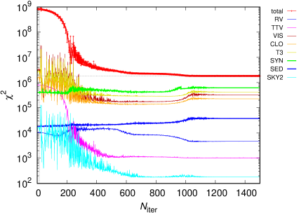
Figure 4: Example of convergence for the alternative model (see Tab. 2). All datasets (RV, TTV, VIS, CLO, T3, SYN, SED, SKY2) were taken into account, with alternative weights $w_{\rm rv}=100$, $w_{\rm ttv}=1000$, $w_{\rm vis}=0.1$, $w_{\rm clo}=0.1$, $w_{\rm syn}=0.1$, $w_{\rm sky2}=1000.0$. In this case, two stellar components (Ac2, Aa2) were ’forced’ to be on the main sequence, which results in ‘tension’ (cf. increase for several $\chi^{2}$ contributions after 800 iteration). On the other hand, the nominal model does not exhibit such tension.

3.1 Survey of parameters

In order to understand, how individual datasets constrain the model, and to find a global minimum of $\chi^{2}$, we perfomed a survey of parameters. We converged 81 different models. Every convergence was initialized with a different combination of masses $m_{1}$, $m_{2}$ (Ac1, Ac2), within in the range $15$ to $50\,M_{\rm S}$, while $m_{3}$ (Aa1) was set to $m_{\rm sum}-m_{1}-m_{2}-m_{4}$; nevertheless, all parameters were free during convergence. The maximum number of iterations was set to 1000. To speed up this computation, we used a set of predefined synthetic spectra. We assumed unit weights, with the exception of $w_{\rm syn}=0.1$. The radiative parameters of the fourth spectrally undetected component (Aa2) were constrained by Harmanec (1988) parametric relations $m_{4}(T_{4})$, $\log g_{4}(T_{4})$, i.e., assuming it is a normal main-sequence object. The component is too faint to significantly contribute to the total flux, it is, however, not negligible from the dynamical point of view.

The results are shown in Fig. 5. One can clearly see ’forbidden regions’, where no solution can be found ($\chi^{2}$ remains high). For high $m_{1}$, $m_{2}$, this is especially due to the CLO and VIS datasets, which strongly constrain the relative luminosities of (Ac1+Ac2), (Aa1+Aa2) components. Moreover, there are strong correlations between parameters — for TTV negative, for RV positive. This is very useful, because the best-fit model is just at the ‘intersection’. Finally, the $\chi^{2}$ contribution due to the SED dataset seems to be too flat, however, this is because all models were converged, and the distance around 2800 pc corresponds the SED. It does not mean that the SED is unimportant!

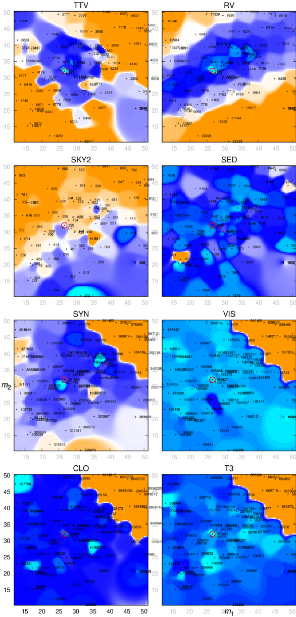
Figure 5: Contributions to $\chi^{2}$ for a set 81 best-fit models. Individual contributions (datasets) are shown in the panels (from top left): TTV, RV, SKY2, SED, SYN, VIS, CLO, T3. Every convergence was initialized with a different combination of masses $m_{1}$, $m_{2}$ (Ac1, Ac2), within in the range $15$ to $50\,M_{\rm S}$, while $m_{3}$ (Aa1) was set to $m_{\rm sum}-m_{1}-m_{2}-m_{4}$; nevertheless, all parameters were free during convergence. Axes correspond to the masses $m_{1}$, $m_{2}$, colours to $\chi^{2}$ (cf. tiny numbers), with adapted colour scales: cyan the very best fit for dataset, blue good fits (${<}\,1.2\min\chi^{2}$), orange poor fits (${\geq}\,1.2\min\chi^{2}$). The factor was 3.0 for TTV, RV, SKY2. ’Forbidden regions’ can be clearly seen (e.g., high $m_{1}$, $m_{2}$ especially due to CLO), as well as correlations between parameters (TTV $-$, RV $+$). The weighted very best fit for all datasets is denoted by red circle.

3.2 Nominal model

The best-fit parameters of our nominal model are listed in Tab. 2. Observed and synthetic data are then compared in numerous Figs. 6 to 14.

First, the eclipse-timing variations (Fig. 6) exhibit much smaller amplitudes compared to Mayer et al. (2022), because they are suppressed by the actual motion of the eclipsing binary (Ac1+Ac2). The respective $\chi^{2}_{\rm ttv}$ contribution is still larger than the number of data points $n_{\rm ttv}$, because one has to fit other datasets at the same time (RV); the result is a compromise.

Second, the radial velocities of the eclipsing binary Ac1+Ac2 (Fig. 7) show some systematics related to Ac1 component at the phases 0.0, 0.5 (i.e., primary and secondary eclipses), when lines are blended and RVs should be close to zero. Additional systematics are present elsewhere, e.g., between 0.6-0.7, which cannot be avoided due to other RV measurements with relatively low RV values. A reason might be hidded in a complex reduction and rectification procedure; one possible solution would be to prefer fitting of synthetic spectra, instead of deriving RVs. (See also Section 3.4.) Regarding Ac2 component, which is relatively faint and fast-rotating, a number of measurements is offset. Because these substantially contribute to $\chi^{2}_{\rm rv}$, we decided to remove RVs of Ac2 in the alternative model (see below).

Third, the RVs of Aa1 component (Fig. 8) seem to be reliable, because it is relatively bright and slow-rotating. Yet, both Aa1 and Ac1 RVs are clearly affected by the wide orbit ((Ac1+Ac2)+(Aa1+Aa2)). This was detected in Mayer et al. (2022) as variable $\gamma$ velocities. The fourth component Aa2 is too faint, but its predicted maximum RV should be of the order of ${\pm}\,300\,{\rm km}\,{\rm s}^{-1}$.

Astrometry of the wide orbit (Ac+Aa ‘binary’; Fig. 9) provides a fundamental angular scale, which together with ETVs and RVs constrains the fundamental parameters. Even though there is some ‘tension’ between periods from RVs and ETVs (Mayer et al., 2022), we regard the resulting period $P_{3}=(14722\pm 50)\,{\rm d}$ as a reasonable compromise.

The blue part (399–544 nm) of the eight rectified FEROS spectra (with high signal-to-noise ratio) were also fitted (Fig. 10). The $\chi^{2}_{\rm syn}$ contribution is still substantial, mostly because the level of continuum was not always correctly determined. H$\beta$, H$\gamma$ lines were removed from the fitting procedure due to strong emission features; impossible to be fitted by our model, which does not include any optically-thin circumstellar matter (CSM). We can only fit weak emission lines (e.g., Fe III), present in synthetic spectra of stellar atmospheres. On the other hand, H$\delta$ does have features (asymmetries), which are reasonably fitted, although the depths of synthetic hydrogen lines are not matched precisely, which is –again– related to the level of surrounding continuum (for example, between 405.1 to 412.6 nm there is no continuum, as verified by synthetic spectra). Nevertheless, the depths as well as features of He I, C II, O II, Mg II lines are fitted much better. Overall, the determination of the respective RVs is very precise (especially for Ac1, Ac2 components), because we fit all lines at the same time (a.k.a. cross-correlation). Our model also naturally couples all spectra (by the orbits), which avoids line blends.

Regarding the SED (Fig. 11), the fit is acceptable, within $\pm 0.2\,{\rm mag}$ in the NUV–NIR range, which is likely related to the uncertainties of dereddening (described in Sec. 2.1). Moreover, 0.15 mag is the depth of minima. The FIR range is not fitted, without any CSM, which would indeed increase the respective $\chi^{2}_{\rm sed}$ contribution. Nevertheless, the SED (together with the masses, radial velocities, angular scale, …) determines the distance around 2800 pc.

A comparison of interferometric observations and our model is straightforward for the squared visibilities $V^{2}$ (Fig. 12). The sinusoidal dependence on the baseline $B/\lambda$ essentially corresponds to a wide binary ((Ac1+Ac2)+(Aa1+Aa2)). Scatter of observed $V^{2}$ is related to the Poisson noise; our synthetic $V^{2}$ are smooth. Because $V^{2}$ values can be very close to $1$ (for a binary), it is important to include observed values which are slightly ${>}\,1$, as well as ${<}\,1$, because only then the mean value is close to $1$. The corresponding precision of astrometry, when all VLTI/GRAVITY measurements are ‘compressed’ to $(u,v)$ coordinates, is of the order of $0.010\,{\rm mas}=10\,\mu{\rm as}$.

The same is true for the closure phases $\arg T_{3}$ (Fig. 13). Similarly as in Sanchez-Bermudez et al. (2017) the dependence on $B/\lambda$ is binary-like.

On contrary, the triple product amplitude (Fig. 14) exhibits some systematics, especially at long baselines ($B/\lambda>4\times 10^{7}$ cycles per baseline); observed values are often close to or even exceed $1$, which seems to be a calibration problem. Nevertheless, the positions of maxima and minima of $|T_{3}|$ as a function of $B/\lambda$ are fitted perfectly, hence we retained the dataset in the nominal model (and we removed it in the alternative model; see Sec. 3.3).

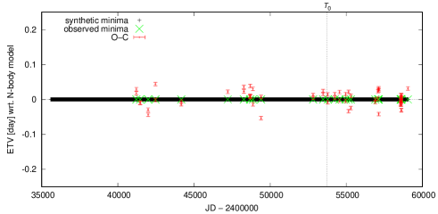
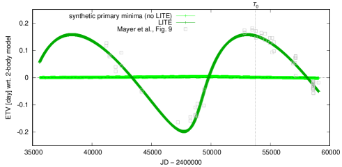
Figure 6: Eclipse timing variations (ETVs) for the nominal model (top; see Tab. 2). All synthetic minima (primary and secondary) are plotted on the $x$ axis (black), together with the observed minima (green) and their difference on the $y$ axis (red). In our N-body model, these ETVs are small, because they are suppressed by the actual motion of the eclipsing binary (Ac1+Ac2) about the centre of mass of all 4 components. For comparison, a simplified two-body model from Mayer et al. (2022), exhibiting large ETVs, is plotted (bottom; gray), with the light-time effect extracted from our N-body model (olive).

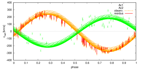
Figure 7: Radial velocities (RVs) of components Ac1 (orange), Ac2 (green). Observed values derived from spectra (Mayer et al. 2022; error bars), synthetic values directly derived from our N-body model (dots) and residuals (red) are plotted. Large residuals are present close to the eclipses (phases 0.0, 0.5), because individual lines (RVs) cannot be reliably separated, as well as for the component Ac2, which has very broad lines (hence uncertain RVs).

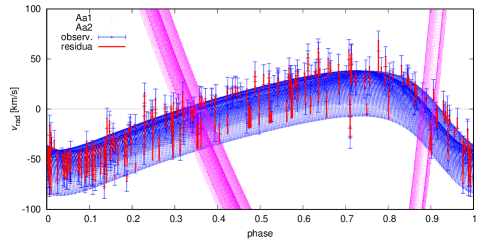
Figure 8: Same as Fig. 7 for components Aa1 (blue), Aa2 (magenta). The spectroscopic binary orbit (Aa1+Aa2) is highly eccentric. The broad range of both synthetic and observed RVs is due to its motion on the wide orbit ((Ac1+Ac2)+(Aa1+Aa2)).

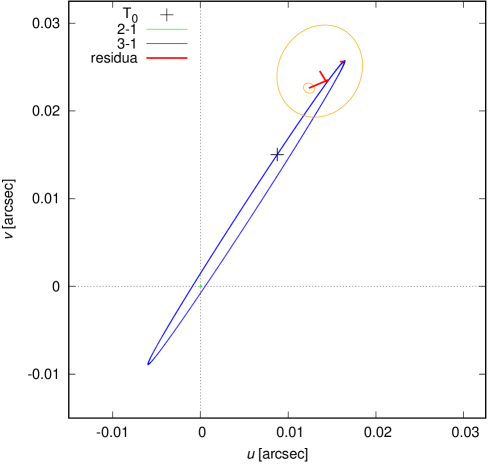
Figure 9: Astrometry derived from previous interferometric measurements (see Tab. 1). Positions of Aa1 components with respect to Ac1 are plotted (blue), as well as Ac2 w.r.t. Ac1 (green; in the very centre). Tiny oscillations visible as thickness of lines are due to photocentre motions. We used positive signs of $(u,v)$ for this plot. The orbit is constrained not only by this astrometry, but also by ETVs and RVs (see Figs. 6, 8).

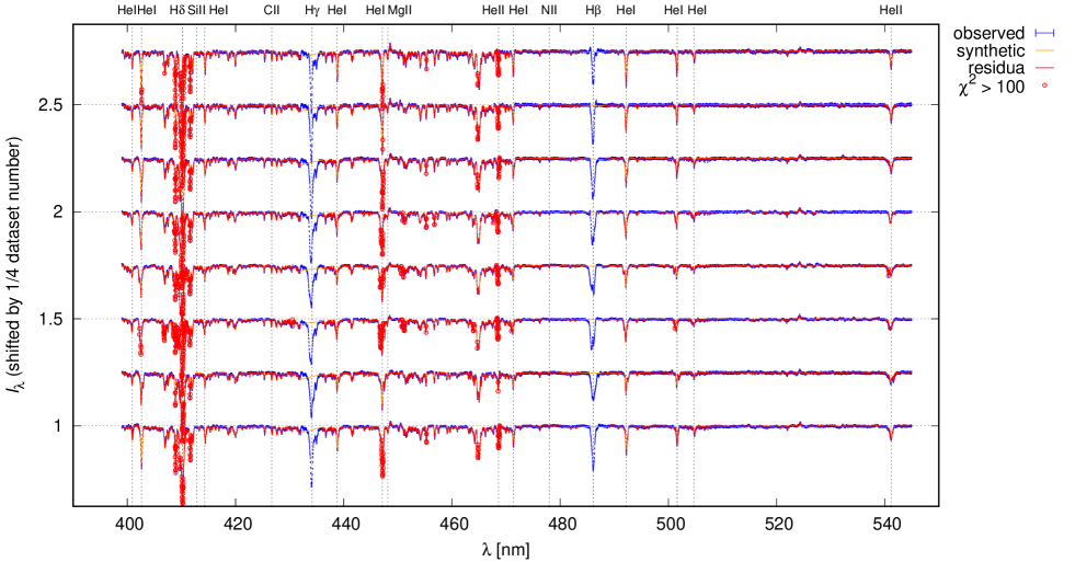
Figure 10: Comparison of the rectified observed FEROS spectra (blue) with the synthetic spectra computed by our N-body model (orange). Residuals are also plotted (red). They are substantial (see circles) for the $H\delta$ line, where the continuum level is uncertain (between 405.1 and 412.6 nm). Nevertheless, most line features (including splits, blends, weak lines close to the continuum) are present in both observed and synthetic spectra, resulting in reliable RVs of individual stellar components (especially Ac1, Aa1; cf. Fig. 15).

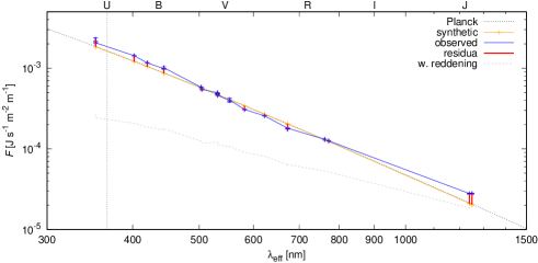
Figure 11: Comparison of the dereddened spectral-energy distribution (SED; blue) and the synthetic SED (red). While the near-ultraviolet to near-infrared region is reasonably described by our N-body model, there is a substantial excess of the observed flux. in the far-infrared region. This is possibly related to non-thermal processes in stellar atmospheres or presence of circumstellar matter, which is not included in our N-body model.

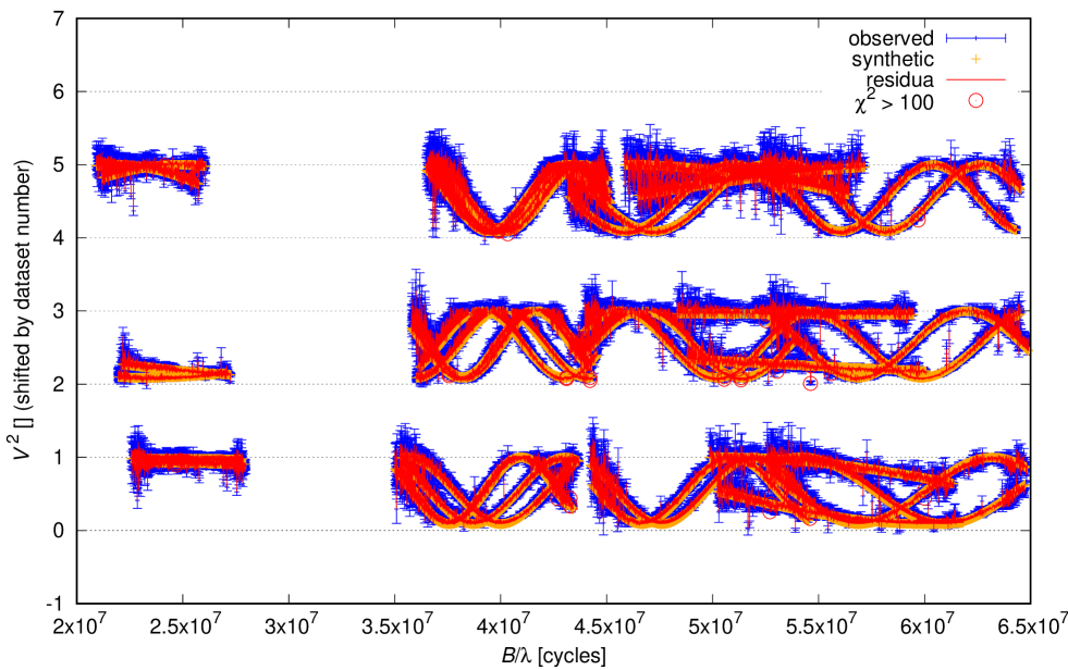
Figure 12: Squared visibilities $V^{2}$ for the VLTI/GRAVITY observations (Mar 14th 2017, Apr 27th 2017; blue), synthetic $V^{2}$ (orange), and residuals (red). The sinusoidal dependence on the baseline $B/\lambda$ essentially corresponds to a wide binary ((Ac1+Ac2)+(Aa1+Aa2)). Disks of individual stellar components cannot be resolved. (at $0.08\,{\rm mas}$, this would correspond a drop of $V^{2}$ by only 0.01 at the longest baseline).

Figure 13: Same as Fig. 12 for the closure phase $\arg T_{3}$. Again, the dependence on $B/\lambda$ is binary-like.

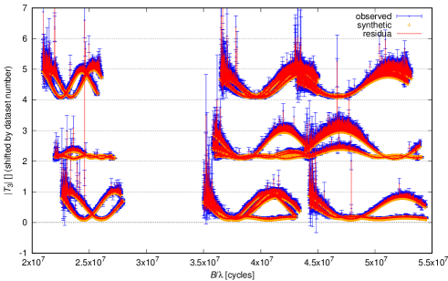
Figure 14: Same as Fig. 12 for the triple product amplitude $|T_{3}|$. Observed values are often close to or even exceed $1$, which indicates a possible calibration problem at long baselines ($B/\lambda>4\times 10^{7}$ cycles per baseline); synthetic values are always ${<}\,1$. Nevertheless, the positions of maxima and minima of $|T_{3}|(B/\lambda)$ are fitted perfectly.

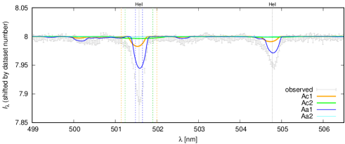
Figure 15: Synthetic spectra of individual components (Ac1, Ac2, Aa1, Aa2) weighted by their luminosities, so that one can see their contributions to the total spectrum. For comparison, the observed spectrum is plotted (error bars). The region of He I 5016 and 5047 lines is plotted. Ac2 component is fast-rotating and has broad lines, Aa2 component is not luminous and its contribution is negligible.

3.3 Alternative model

Alternative models are useful to determine the true uncertainties of parameters. With this goal in mind, we modified a number of things, in particular, RVs of Ac2 component were not used, because they did not seem reliable. Instead, Ac2 component was again constrained according to Harmanec (1988). In case of RVs of Ac1, we removed outliers identified in the nominal model.

Similarly, $|T_{3}|$ was not used, because it exhibited systematics at long baselines, while $V^{2}$ at the same baselines was fitted precisely. Outliers were also removed from the VIS, CLO, and T3 datasets, as they often occur at the beginning of the ‘burst’, so that we assume they were caused by temporarily erroneous setup.

The weights were set as ‘extreme’, to enforce fitting of datasets with low number of points: $w_{\rm rv}=100$, $w_{\rm ttv}=1000$, $w_{\rm vis}=0.1$, $w_{\rm clo}=0.1$, $w_{\rm syn}=0.1$, $w_{\rm sky2}=1000.0$. On contrary, we relaxed the SED constraint by using $w_{\rm sed}=1$.

The results are summarized in Tab. 2 and Figures were moved to Appendix A. Major differences between the models can summarized as follows. Using Harmanec (1988) means forcing Ac2 component to be on the main sequence. Since we needed a substantial mass ratio to explain RVs of Ac1, the temperature of Ac2 increases (and its radius decreases). Putting less weight on the SED means that the distance is allowed to decrease (down to 2500 pc), at the expense of systematic differences in the V–NIR region. ETVs are more centered with respect to zero $O-C$ value, including a group of measurements at ${\rm JD}\simeq 2458570$. RVs and astrometry of Aa1 indicate that the eccentricity of the wide orbit is still uncertain ($\log e_{3}=-0.28$ vs. $-0.54$). A comparison of observed and synthetic spectra shows somewhat larger systematics for He I lines. For interferometric quantities ($V^{2}$, $\arg T_{3}$), we detect only minor shifts, in $B/\lambda$, and offsets in amplitudes of the closure phase.

Even though the alternative model exhibits larger total $\chi^{2}$, it is a viable alternative and we can use it to estimate uncertainties (see Tab. 2; last column).

3.4 A note on oblateness

Oblateness of components may also contribute to the precession of orbits. It can be characterized by the Love number $k_{2}$, the rotation period $P$, and the body radius $R$ (as in Fabrycky 2010), or alternatively by a series of multipoles $C_{\ell,m}$, $S_{\ell,m}$ if the respective shape is more complex (as in Brož et al. 2021a). For binary stars, $k_{2}$ is primarily determined by the density profiles and the Roche potential (Claret, 2004). For ‘soft’ bodies, with the polytropic index $n=3$ to $4$, the expected value is of the order $10^{-2}$ to $10^{-3}$ (Yip & Leung, 2017); it’s even less for evolved stars with extended envelopes.

According to our computations, the oblateness with $k_{2}=10^{-3}$ increases $\chi^{2}_{\rm ttv}$ up to 5660, but it can be compensated by slightly adjusting the period $P_{1}$. Only if $k_{2}$ reaches ${\sim}\,0.003$ for Ac1 component, which is probably the upper limit, because $\log g_{1}\lesssim 3.5$, it would increase the precession rate $\dot{\omega}_{1}$, hence $\chi^{2}_{\rm ttv}$ as well as $\chi^{2}_{\rm rv}$. Interestingly, the difference appears to be of the same order as the systematics of RVs mentioned in Section 3.2. Nevertheless, the precession is not so substantial, observed RV curves do not exhibit a clear temporal trend, but rather a scatter (Mayer et al., 2022), and thus all the parameters (except $P_{1}$) remain the same, within uncertainties.

4 Discussion

Compared to previous works on QZ Car (Walker et al., 2017; Blackford et al., 2020), our new model indicates a higher total mass ($137$ vs. $112\,M_{\rm S}$) and a different distribution of masses within the binaries Aa1+Aa2, Ac1+Ac2, preferring the mass ratios Aa1/Aa2 ${\simeq}8$, and Ac1/Ac2 close to 1, respectively.

Given the photo–spectro–interferometric distance of $(2800\pm 100)\,{\rm pc}$ for the nominal model, QZ Car is likely related to the Carina Nebula (NGC 3372). However, when cluster distances were determined from the Gaia early data release 3 parallaxes (Shull et al., 2021; Göppl & Preibisch, 2022), they turned out to be systematically smaller, possibly due to anomalous extinction, with $R_{V}\equiv A_{V}/E(B-V)=3.2$ to $4.0$. For Collinder 228, the median distance is 2470 pc and the angular size about $14^{\prime}$, which corresponds to the tangential size of only $10\,{\rm pc}$. (The radial size is not well constrained by parallaxes.) This revised distance is in accord with our alternative model of QZ Car.

Massive multiple stars in this region may shed light on possible progenitors of the $\eta$ Carinæ event (Weigelt et al., 2016), which was suggested to be caused by mass transfer in triple systems, eventually leading to an explosive merger (Smith et al., 2018). Notably, QZ Car quadruple system includes the eclipsing mass-transferring binary Ac1$\rightarrow$Ac2, which will evolve substantially. According to our model, the mass ratio Ac2/Ac1 is relatively close to 1; it means that we observe this binary almost at its closest distance. If the final mass of Ac1 will decrease to, e.g., $5\,M_{\rm S}$, the angular momentum conservation implies the final separation (as well as the envelope extent of Ac1; Paxton et al. 2015), of the order of $1\,000\,R_{\rm S}$, i.e., substantially less than the pericentre of (Aa1+Aa2)+(Ac1+Ac2) binary, $a_{3}(1-e_{3})=6\,300\,R_{\rm S}$. This does not lead to an imminent instability. It is still unclear, what has been (and shall be) the role of loosely bound companions, Ab, Ad, B, C, D, imaged around QZ Car (Rainot et al., 2020), because we still lack their proper motions.

5 Conclusions

Using Mayer et al. (2022) observation-specific models as initial conditions for convergence, we constructed a robust N-body model of the QZ Car quadruple system, fitting all three orbits and stellar–radiative parameters at the same time. Because we used all types of observations, which are in a sense orthogonal, the model is well-behaved and does not exhibit strong correlations (‘drifts’). Independent constraints for individual parameters were only used when needed (e.g., for the luminosity–radius of Aa2 component, which is too faint to be directly observable in the flux).

Our preferred model is the nominal one (see Tab. 2); the best-fit masses are $m_{1}=26.1\,M_{\rm S}$, $m_{2}=32.3\,M_{\rm S}$, $m_{3}=70.3\,M_{\rm S}$, $m_{4}=8.8\,M_{\rm S}$, with uncertainties of the order of $2\,M_{\rm S}$, and the distance $d=(2800\pm 100)\,{\rm pc}$. The alternative model, with Ac2 component ‘forced’ to be on the main sequence, exhibits some systematic differences, especially for the SED, which can be attributed to anomalous extinction with $R_{V}\sim 3.4$. We used it to determine realistic uncertainties of parameters.

There are still some poorly constrained parameters, in particular, the mutual inclinations of the orbits, because the longitude of nodes $\Omega_{1}$ is not constrained by eclipses. For simplicity, we assumed a co-planarity, but observations with the VLTI/GRAVITY instrument covering both short periods ($P_{1}$, $P_{2}$) could be used to constrain it, because astrometric uncertainties related to Aa1 component are of the same order as the photocentre motions related to the eclipsing binary Ac1+Ac2.

As a future work, we suggest to include also the observed light curve and strong emission lines (especially, H$\alpha$, H$\beta$) in the model. However, this is generally difficult, given a possible presence of both optically-thick and optically-thin circumstellar matter (CSM). An appropriate treatment of the radiation transfer in the CSM in needed for this purpose (e.g., Brož et al. 2021b). Moreover, a presence of oscillatory signals in the TESS light curve also requires substantial model improvements (e.g., Conroy et al. 2020).

Table 2: Best-fit parameters for the nominal (Sec. 3.2) and alternative (Sec. 3.3) models.

		nominal	alternative
comp.	var.	val.	val.	unit	$\sigma$
Ac1	$m_{1}$	$25.5$	$31.4$	$M_{\rm S}$	$2$
Ac2	$m_{2}$	$33.2$	$34.8^{\dagger}$	$M_{\rm S}$	$2$
Aa1	$m_{3}$	$69.8$	$55.2$	$M_{\rm S}$	$5$
Aa2	$m_{4}$	$8.85^{\dagger}$	$10.3^{\dagger}$	$M_{\rm S}$	$2$
Ac1+Ac2	$P_{1}$	$5.998599$	$5.998601$	day	$0.000002$
	$\log e_{1}$	$-2.876$	$-3.492$	1	$1$
	$i_{1}$	${\bf+93.0}$	$-93.0$	deg	$1.0$
	$\Omega_{1}$	${\bf 326.5}$	$146.0$	deg	$1.0$
	$\varpi_{1}$	$343.4$	$15.9$	deg	$10.0$
	$\lambda_{1}$	$266.4$	$265.6$	deg	$1.0$
Aa1+Aa2	$P_{2}$	$20.734367$	$20.734963$	day	$0.000050$
	$\log e_{2}$	$-0.382$	$-0.451$	1	$0.1$
	$i_{2}$	${\bf+93.0}$	$-93.0$	deg	$1.0$
	$\Omega_{2}$	${\bf 326.0}$	$146.0$	deg	$1.0$
	$\varpi_{2}$	$83.8$	$79.2$	deg	$10.0$
	$\lambda_{2}$	$306.3$	$305.3$	deg	$1.0$
Ac+Aa	$P_{3}$	$14728$	$14645$	day	$100$
	$\log e_{3}$	$-0.268$	$-0.516$	1	$0.1$
	$i_{3}$	${\bf+92.1}$	$-93.2$	deg	$1.0$
	$\Omega_{3}$	${\bf 326.7}$	$146.8$	deg	$1.0$
	$\varpi_{3}$	$295.7$	$296.5$	deg	$10.0$
	$\lambda_{3}$	$53.3$	$50.8$	deg	$1.0$
Ac1	$T_{1}$	$29687$	$31894$	K	$1000$
Ac2	$T_{2}$	$32979$	$43349$	K	$1000$
Aa1	$T_{3}$	$29564$	$27705$	K	$1000$
Aa2	$T_{4}$	$23446$	$25329$	K	$1000$
Ac1	$\log g_{1}$	$3.40$	$3.69$	cgs	$0.1$
Ac2	$\log g_{2}$	$3.80$	$3.92^{\dagger}$	cgs	$0.1$
Aa1	$\log g_{3}$	$3.37$	$3.35$	cgs	$0.1$
Aa2	$\log g_{4}$	$4.10^{\dagger}$	$4.10^{\dagger}$	cgs	$0.1$
Ac1	$v_{\rm rot1}$	$121$	$129$	${\rm km}\,{\rm s}^{-1}$	$10$
Ac2	$v_{\rm rot2}$	$410$	$310^{\rm f}$	${\rm km}\,{\rm s}^{-1}$	$100$
Aa1	$v_{\rm rot3}$	$109$	$117$	${\rm km}\,{\rm s}^{-1}$	$10$
Aa2	$v_{\rm rot4}$	$100^{\rm f}$	$100^{\rm f}$	${\rm km}\,{\rm s}^{-1}$	–
	$\gamma$	$-10.0$	$-13.6$	${\rm km}\,{\rm s}^{-1}$	$5$
	$d_{\rm pc}$	$2836$	$2452$	pc	$100$
	$n_{\rm rv}$	$491$	$491$
	$n_{\rm ttv}$	$64$	$64$
	$n_{\rm vis}$	$54394$	$54394$
	$n_{\rm clo}$	$41367$	$41367$
	$n_{\rm t3}$	$41367$	–
	$n_{\rm syn}$	$36800$	$36800$
	$n_{\rm sed}$	$32$	$32$
	$n_{\rm sky2}$	$12$	$12$
	$\chi^{2}_{\rm rv}$	$4210$	$4142$
	$\chi^{2}_{\rm ttv}$	$1133$	$944$
	$\chi^{2}_{\rm vis}$	$165821$	$176818$
	$\chi^{2}_{\rm clo}$	$128730$	$125861$
	$\chi^{2}_{\rm t3}$	$296025$	–
	$\chi^{2}_{\rm syn}$	$269954$	$291833$
	$\chi^{2}_{\rm sed}$	$7590$	$19144$
	$\chi^{2}_{\rm sky2}$	$349$	$59.4$
	$\chi^{2}$	$630856$	$1759054^{\rm w}$

Table 3: Derived parameters for the nominal and alternative models.

		nominal	alternative
comp.	var.	val.	val.	unit	$\sigma$
Ac1+Ac2	$a_{1}$	$54.032$	$56.226$	$R_{\rm S}$	$1$
Aa1+Aa2	$a_{2}$	$136.132$	$128.052$	$R_{\rm S}$	$10$
Ac+Aa	$a_{3}$	$13053$	$12820$	$R_{\rm S}$	$100$
Ac1+Ac2	$e_{1}$	$0.001$	$0.0003$	$1$	$0.01$
Aa1+Aa2	$e_{2}$	$0.414$	$0.353$	$1$	$0.1$
Ac+Aa	$e_{3}$	$0.539$	$0.304$	$1$	$0.1$
Ac1	$R_{1}$	$16.626$	$13.229$	$R_{\rm S}$	$1$
Ac2	$R_{2}$	$11.975$	$10.592$	$R_{\rm S}$	$1$
Aa1	$R_{3}$	$28.286$	$25.962$	$R_{\rm S}$	$1$
Aa2	$R_{4}$	$4.340$	$4.727$	$R_{\rm S}$	$1$
Ac1	$L_{1}$	$0.220$	$0.192$	$1$	$0.05$
Ac2	$L_{2}$	$0.133$	$0.189$	$1$	$0.05$
Aa1	$L_{3}$	$0.635$	$0.600$	$1$	$0.02$
Aa2	$L_{4}$	$0.010$	$0.017$	$1$	$0.01$

Appendix A Figures for the alternative model

For comparison, we show corresponding Figures for the alternative model (Fig. 16 to Fig. 23). Generally, they are similar to the nominal model, but they demonstrate, how weights and additional constraints (for Ac2, Aa2 components) can change the best-fit solution.

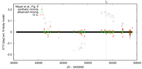
Figure 16: Same as Fig. 6 for the alternative model.

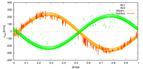
Figure 17: Same as Fig. 7 for the alternative model.

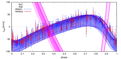
Figure 18: Same as Fig. 8 for the alternative model.

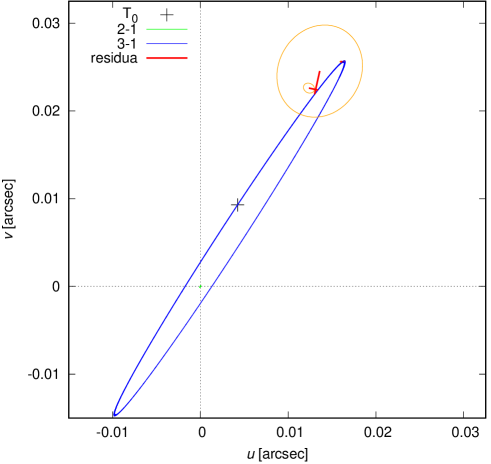
Figure 19: Same as Fig. 9 for the alternative model.

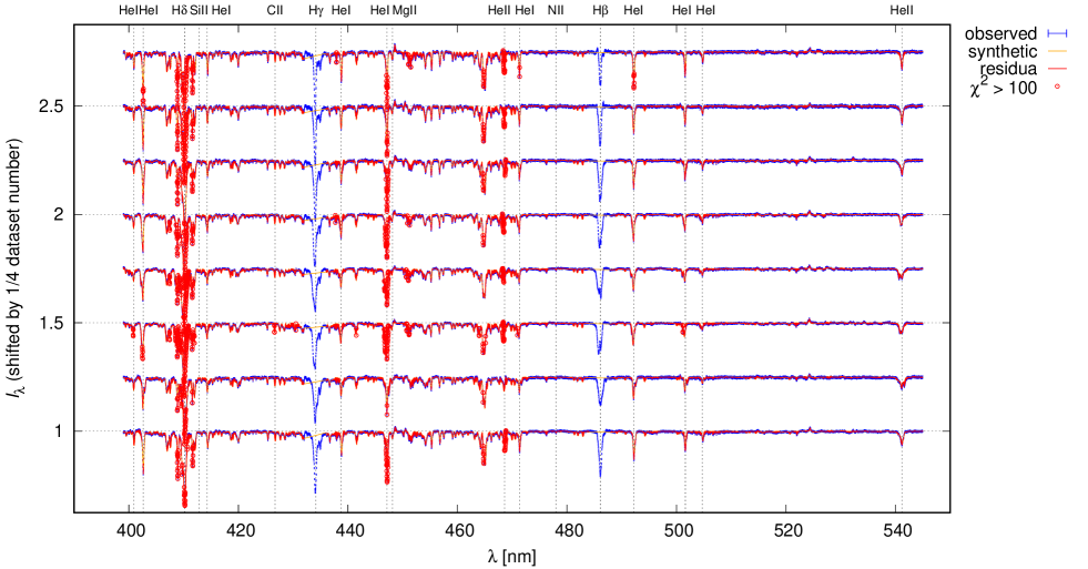
Figure 20: Same as Fig. 10 for the alternative model.

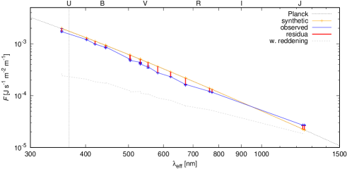
Figure 21: Same as Fig. 11 for the alternative model.

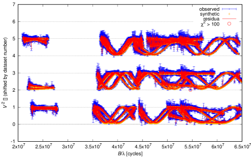
Figure 22: Same as Fig. 12 for the alternative model.

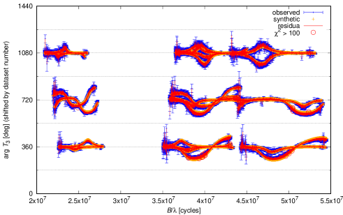
Figure 23: Same as Fig. 13 for the alternative model.