¹¹institutetext: Université Paris Cité, Institut de Physique du globe de Paris, CNRS UMR 7154, F-75005 Paris, France ²²institutetext: LGL-TPE - Laboratoire de Géologie de Lyon - Terre, Planètes, Environnement, Lyon, France

On the Nature and Origin of Atmospheric Annual and Semi-annual Oscillations

V. Courtillot 11 J-L. Le Mouël 11 F. Lopes 11 D. Gibert 22

This paper proposes a joint analysis of variations of global sea-level pressure (SLP) and of Earth’s rotation RP, expressed as the coordinates of the rotation pole ( $m_{1}$ , $m_{2}$ ) and length of day (lod). We retain iterative singular spectrum analysis (iSSA) as the main tool to extract the trend, periods and quasi periods in the data time series. SLP components are a weak trend, eleven quasi-periodic or periodic components ( $\sim$ 130, 90, 50, 22, 15, 4, 1.8 yr), an annual cycle and its first three harmonics. These periods are characteristic of the space-time evolution of the Earth’s rotation axis (RP) and are present in many characteristic features of solar and terrestrial physics. The amplitudes of the annual SLP component and its 3 first harmonics decrease from 93 hPa for the annual to 21 hPa for the third harmonic. In contrast, the components with pseudo-periods longer than a year range between 0.2 and 0.5 hPa. The trend (21 hPa) could be part of the 90 yr Gleissberg cycle. We focus mainly on the annual and to a lesser extent semi-annual components. The annual RP and SLP components have a phase lag of 152 days (half he Euler period) and they have similar envelopes, offset by about 40 years: polar motion leads atmospheric pressure. Maps of the first three components of SLP (that together comprise more than 85% of the data variance) reveal interesting symmetries. The trend is very stable and forms a triskel structure that can be modeled as Taylor-Couette flow of mode 3. The annual component is characterized by a large negative anomaly extending over Eurasia in the NH Summer (and the opposite in the NH Winter) and three large positive anomalies over Australia and the southern tips of South America and South Africa in the SH Spring (and the opposite in the SH Autumn) forming a triskel. The semi-annual component is characterized by three positive anomalies (an irregular triskel) in the NH Spring and Autumn (and the opposite in the NH Summer and Winter), and in the SH Spring and Autumn by a strong stable pattern consisting of three large negative anomalies forming a clear triskel within the 40^∘-60^∘ annulus formed by the southern oceans. A large positive anomaly centered over Antarctica, with its maximum displaced toward Australia, and a smaller one centered over Southern Africa complement the pattern. Analysis of SSA components of global sea level pressure shows a rather simple spatial distribution with the principal forcing factor being changes in parameters of the Earth’s rotation pole and velocity (measured through length of day). The flow can probably best be modeled as a set of coaxial cylinders arranged in groups of three (triskels) or four and controlled by Earth topography and continent/ocean geography. Flow patterns suggested by maps of the three main SSA components of SLP (trend, annual and semi-annual) are suggestive of Taylor-Couette flow. The envelopes of the annual components of SLP and RP are offset by four decades and there are indications that causality is present in the sense from changes in Earth rotation axis force pressure variations.

Key Words.:

Annual and Semi-annual oscillations, Taylor-Couette, Sea Level Pressure

1 Introduction

This paper is an attempt to obtain better constraints on the forcings of the trend and annual components of both global sea-level pressure and variations in the Earth’s rotation, and to test the hypothesis that there might be a causal link between them.

Lopes et al. (2022a) undertook the singular spectral analysis (SSA) of the evolution of mean sea-level atmospheric pressure (SLP) since 1850. In addition to dominant trends, a eleven quasi-periodic components were identified, with (pseudo-) periods of $\sim$ 130, 90, 50, 22, 15, 4, 1.8, 1, 0.5, 0.33, and 0.25 years, corresponding to the Jose, Gleissberg, Hale and Schwabe cycles, to the annual cycle and its first three harmonics. These periods are already known to be characteristic of the space-time evolution of the Earth’s rotation axis: the rotation pole (RP) also undergoes periodic motions longer than 1 year, at least up to the Gleissberg $\sim$ 90 yr cycle (Chandler 1891a, b; Markowitz 1968; Kirov et al. 2002; Lambeck 2005; Zotov et Bizouard 2012; Chao et al. 2014; Zotov et al. 2016; Lopes et al. 2017; Le Mouël et al. 2021; Lopes et al. 2021, 2022a). They are encountered in solar physics (Gleissberg 1939; Jose 1965; Coles et al. 2019; Charvatova et Strestik 1991; Scafetta 2010; Le Mouël et al. 2017; Usoskin 2017; Scafetta 2020; Courtillot et al. 2021; Scafetta 2021) and terrestrial climate (Wood et al. 1974; Mörth et Schlamminger 1979; Mörner 1984; Schlesinger et Ramankutty 1994; Lau and Weng 1995; Courtillot et al. 2007, 2013; Le Mouël et al. 2019a; Scafetta et al. 2020; Connolly et al. 2021).

The rotation velocity is usually expressed as the length of day (lod); it contains periods of 1 year and shorter, but also (though they are weaker) longer periods from 11 yr to 18.6 yr (Guinot 1973; Ray et Erofeeva 2014; Le Mouël et al. 2019b; Dumont et al. 2021; Petrosino et Dumont 1995). Lopes et al. (2022a) showed that the secular variation of lod since 1846 Stephenson et Morrison (1984) and RP have been carried by an oscillation whose period fits the Gleissberg cycle.

RP consists to first order of 3 SSA components that together amount to more than 85% of the total signal variance Lopes et al. (2017): the Markowitz (1968) drift, the Chandler (1891a, b) free oscillation (actually a double component with periods $\sim$ 433 and $\sim$ 434 days), and the forced annual oscillation. Polar drift does not have a universally accepted explanation (Stoyko 1968; Hulot et al. 1996; Markowitz et Guinot 2022; Deng et al. 2021). The two other oscillatory components (Chandler and annual) are obtained using the Liouville-Euler system, that describes the motion of a spherical rotating solid body (e.g. Lambeck (2005), chapter 3, system 3.2.9).

Polar drift has been discussed in Le Mouël et al. (2021) and Lopes et al. (2022a) and the free Chandler wobble in Lopes et al. (2021). In the present paper, we focus on the third major component, the forced annual oscillation. This oscillation is often assumed to be forced by the Earth’s fluid envelopes, hence also by climate variations (e.g. Gross et al. (2003), Lambeck (2005) chapter 7, Bizouard et Seoane (2010); Chen et al. (2019)). The fact that the observed Chandler period (433-434 days) is not equal to the theoretical value of the Euler period (306 days) has been interpreted in terms of Earth elasticity. The annual period is forced by interactions with fluids. Variations in the Sun-Earth distance, hence of the corresponding gravitational forces, displace the fluid atmosphere and ocean; exchanges in angular moment affect RP and lod. The annual oscillation of the rotation pole RP (coordinates $m_{1}$ and $m_{2}$ ) would therefore be due to the presence of the fluid envelopes. If Earth were devoid of fluid envelopes, the annual oscillation should not exist, which would contradict both the theory and observations of motion of a Lagrange top (Landau and Lifchitz 1984). Wilson et Haubrich (1976) recall that Spitaler (1897, 1901) “demonstrated that the annual wobble was forced, at least in part, by the seasonal migration of air masses on and off the Asian continent”. Jeffreys (1916) showed that the annual fluctuation in water storage on the continents was also important. Munk et Mohamed (1961) re-examined the sources of annual wobble excitation and concluded that the air mass effect accounted for much but not all of the annual wobble, and water storage did not explain the remainder. Reservations appear in chapter 7 of Lambeck (2005), Seasonal Variations, page 146, who writes: “The principal seasonal oscillation in the wobble is the annual term which has generally been attributed to a geographical redistribution of mass associated with meteorological causes. Jeffreys, in 1916, first attempted a detailed quantitative evaluation of this excitation function by considering the contributions from atmospheric and oceanic motion, of precipitation, of vegetation and of polar ice. Jeffreys concluded that these factors explain the observed annual polar motion, a conclusion still valid today, although the quantitative comparisons between the observed and computed annual components of the pole path are still not satisfactory”. In summary, the interpretation of the forced annual component of polar motion is still hypothetical and fails to be validated by a numerical model.

In a previous analysis of global sea-level pressure (SLP), we found that trends since 1950 were very stable in time and space (Lopes et al. 2022b) and were organized in a dominant 3-fold symmetry about the rotation axis in the northern hemisphere (NH) and a 3 or 4-fold symmetry in the southern hemisphere (SH) (Lopes et al. 2022b). These features could be interpreted as resulting from Taylor-Couette flow. In this paper, we return to the pressure data and focus on the annual oscillation.

2 The Pressure Data and Method of Analysis

The pressure data are maintained by the Met Office Hadley Centre¹¹1https://www.metoffice.gov.uk/hadobs/hadslp2/data/download.html and can be accessed as maps of global pressure, every month from 1850 up to the Present. The sampling is 5^∘ x 5^∘ ; the data we use are labeled HadSLP2r. Allan et Ansell (2006) have built this series starting with ground observations whose number and location are shown in their Figure 2. These are subjected to a quality check, corrected for various local effects then homogenized with the Empirical Mode Decomposition (EMD) filter.

As in Lopes et al. (2022b), we have used the iterative Singular Spectrum Analysis algorithm (iSSA) to extract the components, mainly the annual one, in each grid cell and as a function of time. For the iSSA method, see Golyandina et Zhigljavsky (2013), for properties of the Hankel and Toeplitz matrices, see Lemmerling and Van Huffel (2001) and for the Singular Value Decomposition (SVD) algorithm, see Golub et Reinsch (1971). For summaries of how we use them, the reader is referred to Lopes et al. (2021).

3 The SSA Pressure Components

We obtain the following components:

The trend (from $\sim$ 1009.15 hPa in 1850 to $\sim$ 1008.35 hPa at present) is the first and largest SSA component. It represents more than 70% of the total variance of the original series. The sequence of the quasi-periodic components is, in decreasing order of periods (amplitudes are in hectoPascal, hPa) :

$\bullet$

$\sim$ 130 years ( $\sim$ 0.7 hPa). We recognize the Jose (1965) cycle,
$\bullet$

$\sim$ 90 yr ( $\sim$ 21 hPa). We recognize the Gleissberg (1939) cycle (Le Mouël et al. 2017),
$\bullet$

$\sim$ 50 yr ( $\sim$ 0.2 hPa),
$\bullet$

$\sim$ 22 yr ( $\sim$ 0.50 hPa). We recognize the Hale cycle (Usoskin et al. 2017),
$\bullet$

$\sim$ 15 yr ( $\sim$ 0.2 hPa). We may recognize an upper bound of the Schwabe (1844), cycle,
$\bullet$

$\sim$ 4 yr ( $\sim$ 0.3 hPa),
$\bullet$

$\sim$ 1.8 yr ( $\sim$ 0.3 hPa).

Then:

$\bullet$

1 yr ( $\sim$ 93 hPa).
$\bullet$

0.5 yr ( $\sim$ 65 hPa).
$\bullet$

0.33 yr ( $\sim$ 44 hPa).
$\bullet$

0.25 yr ( $\sim$ 21 hPa).

4 Annual and Semi-annual SSA Pressure Components and Variations in Polar Motion: Time Analysis

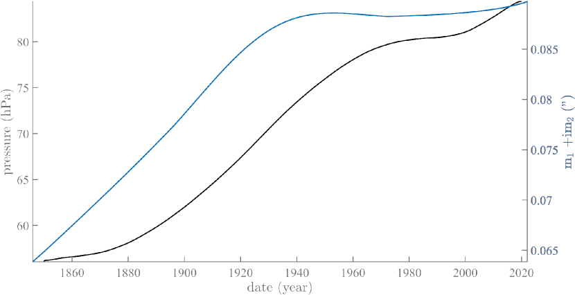
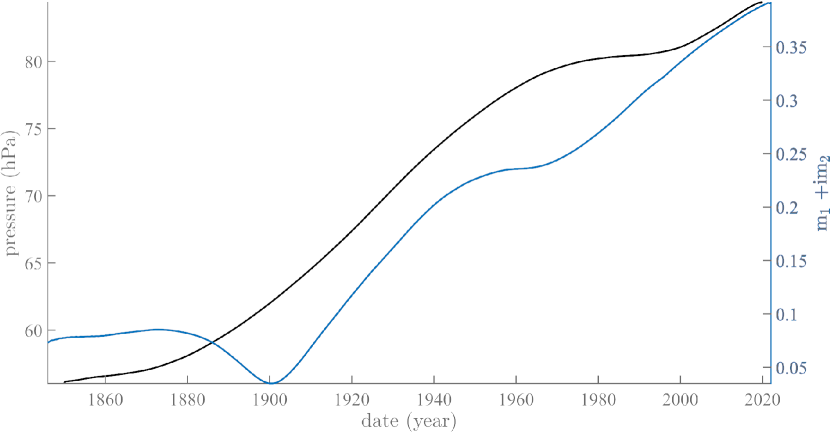
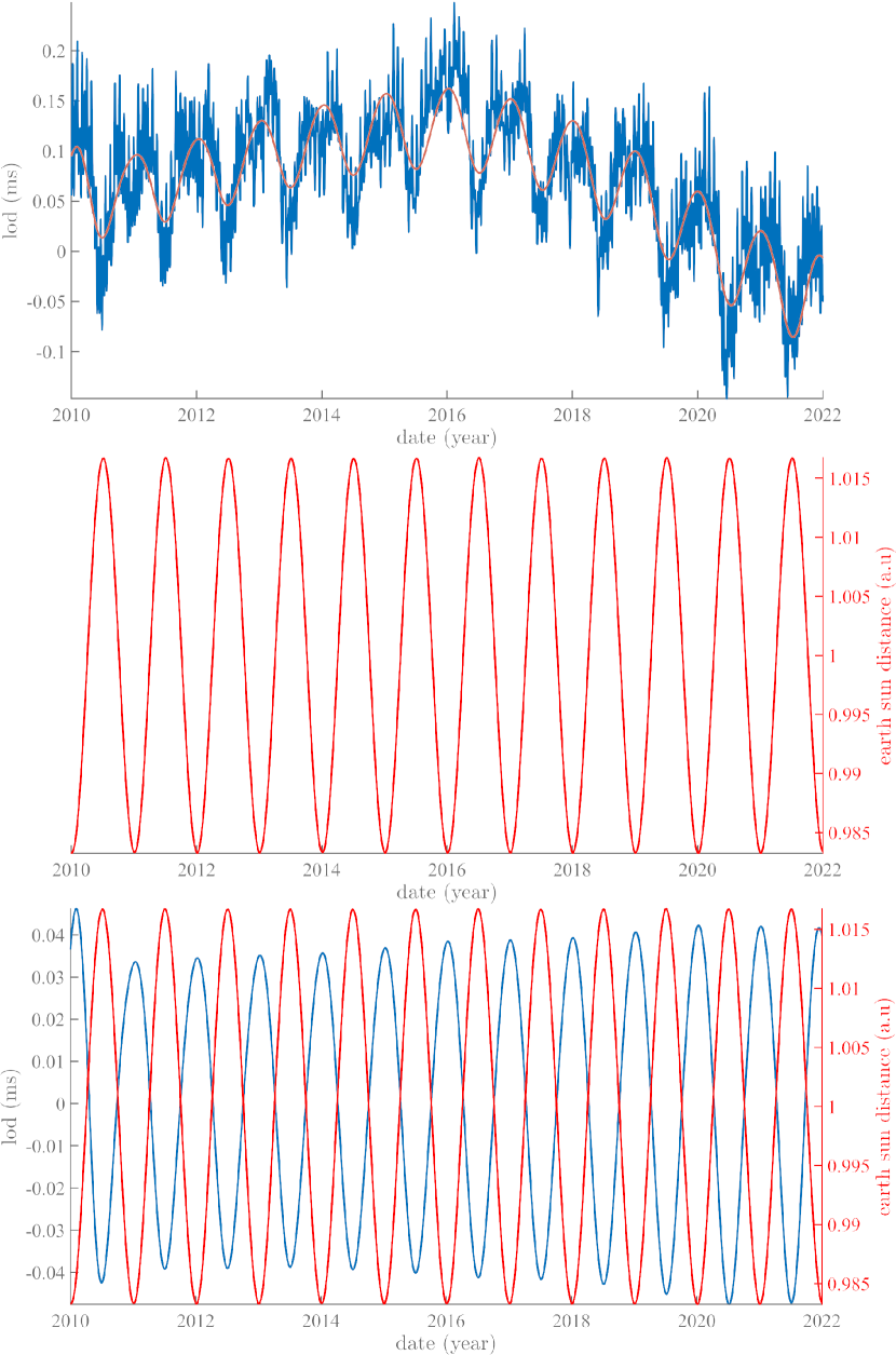
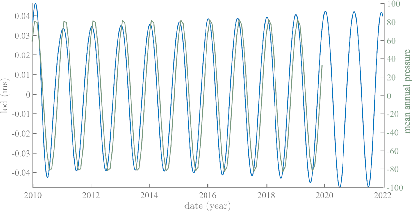
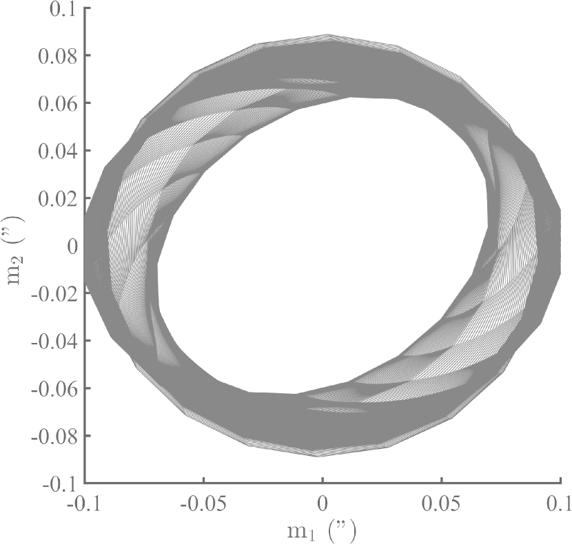
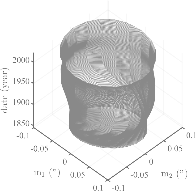
Many studies (e.g. Jeffreys (1916); Lambeck (2005); Adhikari et Ivins (2016)) attempt to relate forced (annual) oscillations to polar motion RP ( $m_{1}$ , $m_{2}$ ) or length of day (lod) (data file EOPC01IAU2000, Vondrák et al. (1995), maintained by IERS²²2 https://www.iers.org/IERS/EN/DataProducts/EarthOrientationData/eop.html). The data are shown and discussed in Lopes et al. (2021). The annual SSA components of $m_{1}$ and $m_{2}$ are displayed in Figure 1. Both undergo some amount of modulation. That modulation is significant for $m_{1}$ , particularly between 1850 and 1930. For $m_{2}$ , it is smaller and more regular. A $m_{1}$ vs $m_{2}$ diagram (see Appendix A) shows the classical Lissajou elliptical shape of annual polar motion. Note that the date of 1930 is when the Chandler wobble undergoes a phase jump of $\pi$ (e.g. Gibert (1998); Gibert et Le Mouël (2008)). The lod data start only in 1962 (not shown, see Lopes et al. (2022a)). The annual and semi-annual SSA components of lod are modulated (Figure 2(a) and Figure 2(b)). The annual component grows slightly until 1990, flattens until 2013 and then starts growing again. The semi-annual component decreases regularly over the sixty years of available data.

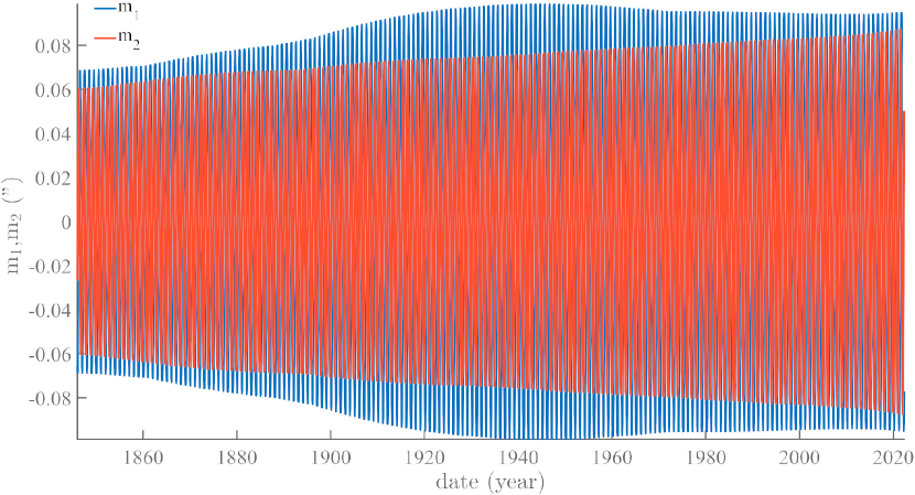
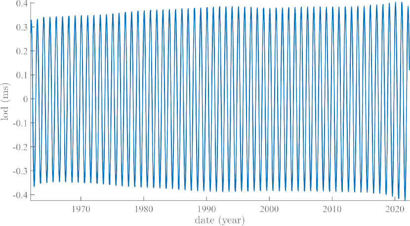
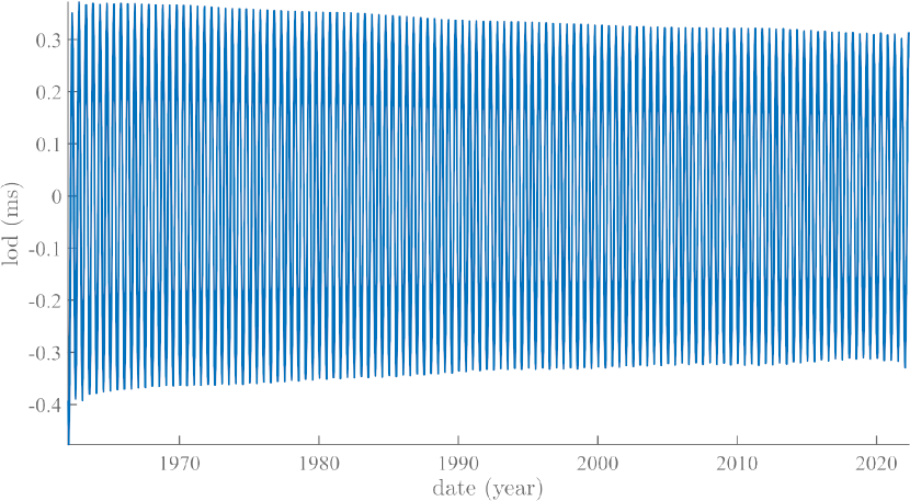
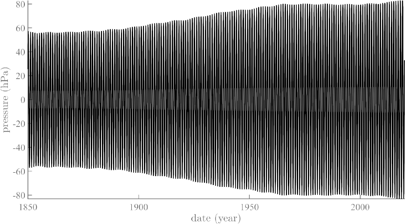
Refer to caption — Figure 1: iSSA annual component of rotation pole coordinates $m_{1}$ and $m_{2}$ from 1850 to the Present.

Figure 3 shows the annual iSSA component since 1850, extracted from the SLP pressure series. Its modulation looks very much like that of $m_{2}$ , with a phase shift (Figure 1). We have checked that the phase shift is constant over the 70 years of data. Its mean value is 152.31 $\pm$ 2.68 days. We have already obtained (exactly) such a phase shift and note that it is (exactly) half of the Euler period of 306 days: a reason for this remains to be found. Using the Hilbert transform, we have determined the envelopes of the two annual components of polar motion and atmospheric pressure (Figure 4(a)). The polar motion clearly precedes pressure by at least 40 years. On Figure 4(b), we see that the trend of polar motion is close to the envelope of pressure, in general preceding it slightly. Given the mathematical properties of the Liouville-Euler set of equations, the potential direction of causality between the two phenomena is in the sense of polar motion leading atmospheric pressure. If correct, this is an important result that confirms Laplace’s statements in his 1799 Traité de Mécanique Céleste (volume 5, chapter 1, page 347; reproduced in Appendix B).

Thus, after applying the Kepler’s law of conservation of areas, Laplace concludes that atmospheric motions do not affect pole rotation.

5 The Annual and Semi-annual SSA Pressure Components: Spatial Analysis

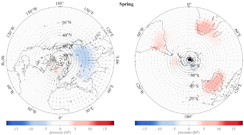
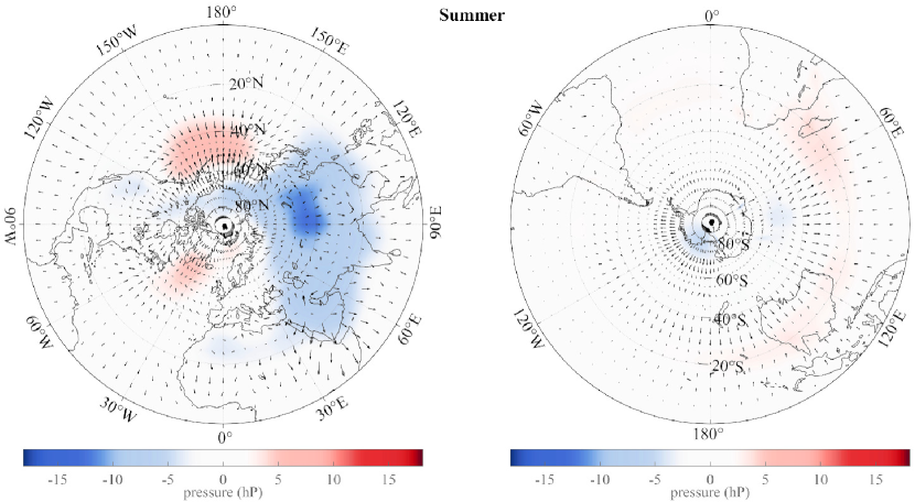
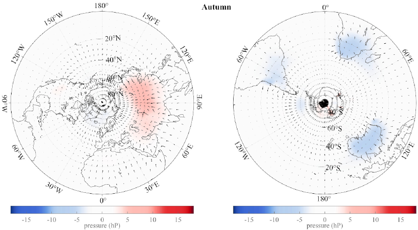
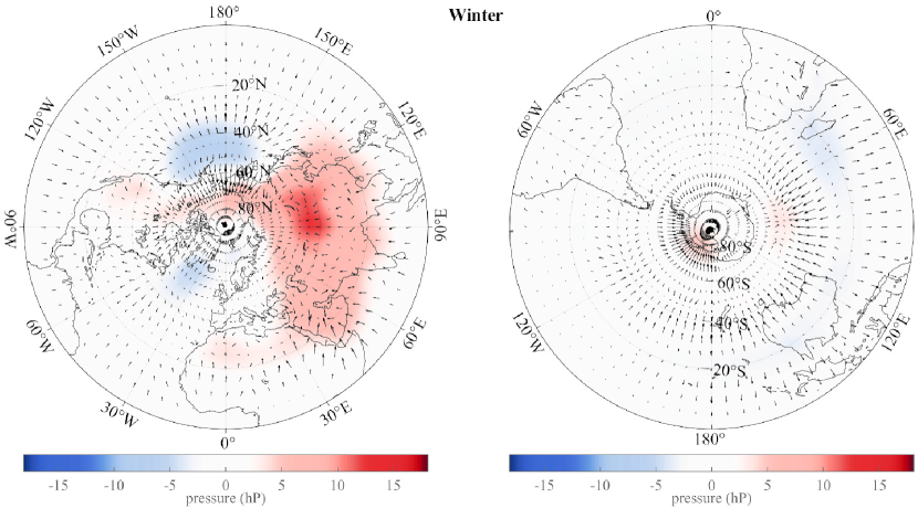
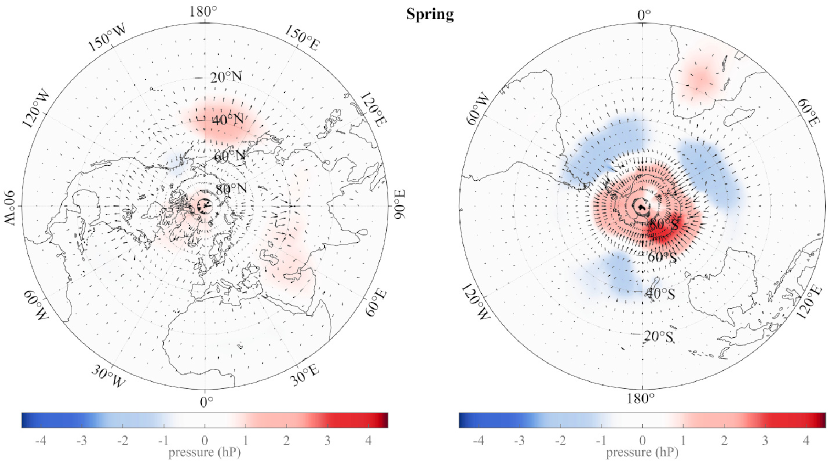
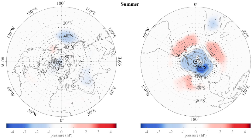
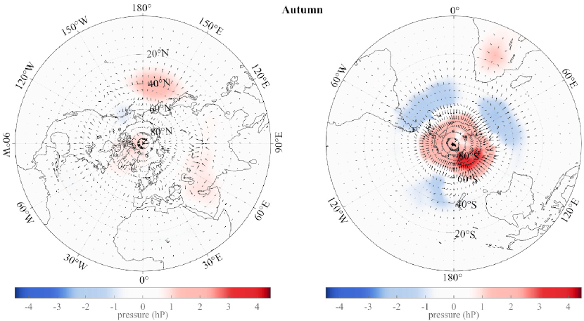
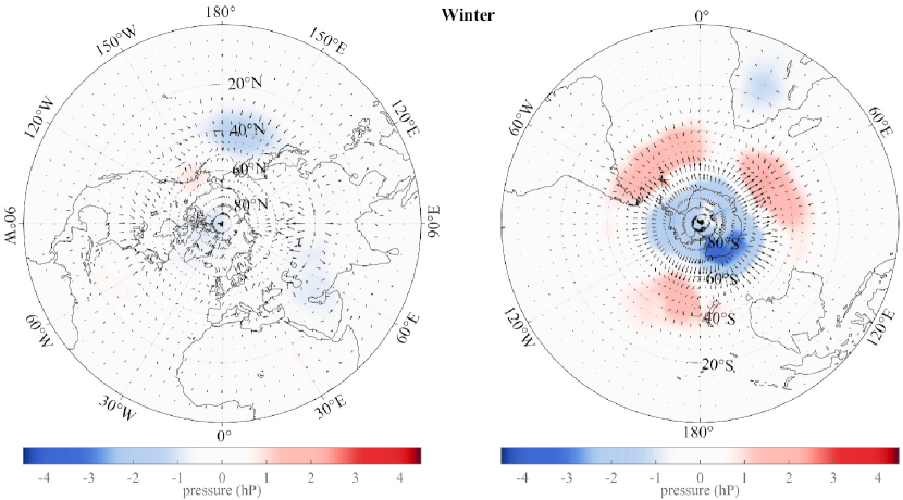
We show in Figure 5 polar maps of the mean amplitude of the annual component (oscillation), for each season since 1850, and in Figure 6 polar maps of the mean of the semi-annual component.

In Figure 5, in the Spring SH, there is a very regular pattern at the intersections of the 20^∘S to 50^∘S annulus and the southern tips of the three southern continents (Africa, Australia and South America). There is a smaller dipole with its negative part centered almost perfectly on the South pole, and its positive part centered on 70^∘S, 105^∘W. In the Fall, the pattern is the same but with a reversal in sign. In the Summer, there is a positive band between 15 and 25°S latitude from Madagascar to New Caledonia (40°-170°E) and a small negative spot near the South pole (Winter is the same with a sign reversal). The positive annulus is actually also seen, much weaker, in the Atlantic and Pacific oceans. The NH is rather different with, in the Spring, a large negative area over Asia from the Red Sea to Japan and extending in latitude from 80^∘N to 15^∘N. This large “anomaly” (using geophysical language) extends negative arms towards Senegal and over the western USA. Over the year, the “anomaly” changes sign. Still in the Summer, there are two sizeable positive anomalies over the northern Atlantic and Pacific Oceans between 40^∘N and 60^∘N. In the SH, the large mean annual pressure variations occur over the Southern continents; in the NH, the Asian continental “anomaly” dominates, though two significant features occur over the northern parts of the oceans. Because the Asian “anomaly” and the two (opposite sign) anomalies in the North Atlantic and Pacific are separated by almost 180° in longitude, their maxima being always in phase, their contributions to the seasonal excitation function tend to cancel (Lamb 1972).

The semi-annual component (Figure 6) has stronger patterns of symmetry. The SH features a very stable 3-fold symmetry (triskel); three large anomalies form an equilateral triangle centered on 70^∘E, 30^∘W and 210^∘W, between latitudes 40^∘S and 60^∘S, a large anomaly of opposite sign is centered on the South Pole (the maximum is actually offset from the SP by 20^∘E towards the 120^∘E meridian), and an anomaly with the same sign as that over the pole, but located over southern Africa. The NH has weaker anomalies forming an irregular triangle with apices near the North Pacific (40^∘N, 165^∘E), Baffin Sea (40^∘N, 50^∘W) and Iran (30^∘N, 60^∘W).

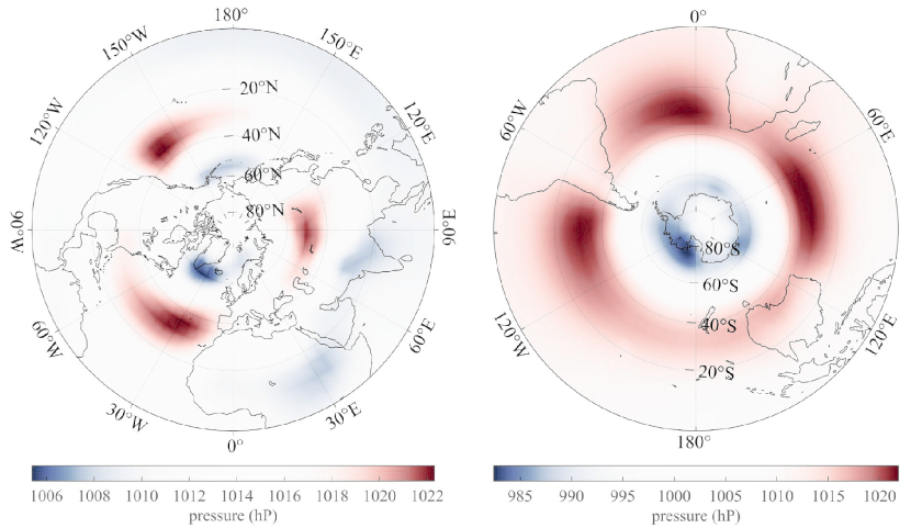
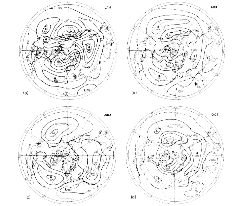
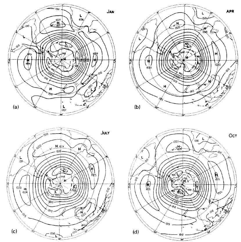
The bottom two maps in Figure 7 are the Spring maps for the annual and semi-annual components. We can compare the maps of Figures 5, 6 and 7 for the annual, semi-annual and trend components with corresponding figures from the reference treatise of Lamb (1972), reproduced in Appendix C .Recall that taken together these three components suffice to capture about 85% of the total signal variance. Figures 4-12 and 4-13 for instance (reproduced in Appendix C as Figures C1aand Figure C1b) show Lamb’s representation of the average mean sea level pressure over (respectively) the northern and southern hemispheres in the 1950s. There is very good agreement for the northern hemisphere (Figure 10(a)): the January map from Lamb and our Winter map show the dominant “dipole” with the large high pressure (HP) over Asia and the low pressure (LP) over the northern Pacific. The April and Spring maps do not agree so well. The July map from Lamb and our Summer map both show a large LP over Asia and two HPs over the northern Pacific and northern Atlantic. The October map from Lamb and our Autumn map show a weaker HP over Asia. For the southern hemisphere (Figure 10(b)), agreement between the two sets of maps is significantly less; the Winter vs January maps both feature a HP centered on Antarctica and a LP extending from Madagascar to Australia, and the reverse in Summer/July. Our Spring (respectively Autumn) maps feature strong HPs (respectively LPs) on the southern tips of the southern continents. This sharp pattern is not really seen so well in Lamb’s (1972) maps (Appendix C).

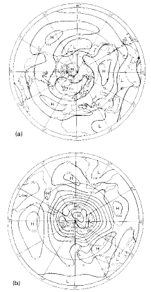
Lamb’s Figure 3-17 (reproduced in Appendix C as Figure C2) represents the annual mean distribution of atmospheric pressure at sea level for the time span 1900-40 for the northern hemisphere and 1900-50s for the southern hemisphere. This can be compared to our maps of the trend (Lopes et al. (2022b), and Figure 7, top row). The agreement is quite good: the 3 fold symmetry of the northern hemisphere and the 4 fold symmetry of the southern hemisphere are even clearer in the Lopes et al. (2022b) maps using the iSSA method to extract the trend (i.e. the main component) from the data. As concluded by Lamb (1972) the effects of geography modify the circumpolar circulation much more in the northern than in the southern hemisphere; “ The broad zonal character of the long-period mean circulation is as permanent as the circumpolar arrangement of the heating and cooling zones and the circumpolar vortex aloft”. It appears to us that such maps are not available in the published literature; the maps from the southern hemisphere are particularly interesting, and so is the triskel in Figure 7 (top left). Specialists may wish to analyze these maps in more detail; they can be provided on simple request.

6 Discussion

6.1 Symmetries and Forcings

We pointed out in a preliminary paper on symmetries of global sea level pressure (Lopes et al. 2022b) that the pattern of Figure 7 was remarkably stable over the 150 years of the data, and that the observed geometry could be modeled as Taylor-Couette flow of mode 3 (NH) or 4 (SH). The remarkable regularity and order three symmetry of the NH triskel occurs despite the lack of cylindrical symmetry of the northern continents. The stronger intensity and larger size of features in the SH is linked to the presence of the annular currents. Following Kepler and Laplace (see above) it appears that the molecules in the atmosphere cannot perturb polar axis motion (“Nous sommes donc assurés qu’en même temps que les vents analysés diminuent ce mouvement, les autres mouvements de l’atmosphère qui ont lieu au-delà des tropiques, l’accélèrent de la même quantité “). The atmosphere behaves as a rotating cylinder undergoing stationary flow. The top of the cylinder is a free surface, the bottom is the surface of the solid crust and/or fluid ocean. This topography interacts strongly with the atmosphere.

6.2 Sun-Earth Distance and Phases

The seasonal change in sign agrees with changes in the Sun-Earth distance. The present values of the ellipticity of the Earth’s orbit and the obliquity of its rotation axis lead to changes of orbital velocity with Summer in the southern hemisphere at perihelion and Summer in the northern hemisphere at aphelion. The torque associated with the Sun changes as velocity changes. As discussed in Lopes et al. (2021, 2022a), forces acting on the polar axis do so through a torque ( $m_{1}$ , $m_{2}$ ) obeying the Liouville-Euler system of equations (from Laplace, 1799). The influence of these torques is in quadrature with the length of day (lod). Changes in orbital velocity of our planet lead to a variation in the solar torque, which acts against the sense of rotation of the planet. Thus, annual variations in lod should be in opposition to changes in the Sun-Earth distance, and they are (Figure 8a, bottom). In the northern latitudes, both the Earth’s rotation and the winds go from West to East, the Earth’s rotation slows in Summer and accelerates in Winter, hence positive pressure anomalies in Winter, negative in Summer. In other words, the pressure anomalies are due to the variation in rotation velocity (tracked through lod changes and winds). The phase difference between the annual components of lod and SLP is constant at 32 $\pm$ 1.2 days (Figure 8b). Relative variations of amplitudes should be similar and indeed they are (Figure 8b).

7 Sketch of a Mechanism

Because more than 70% of the total signal variance is captured by the trend of the atmospheric pressure, that varies by only 1 per mil since 1850, one can resort to the theory of turbulent flow in the case of infinitesimal perturbations (cf. Landau and Lifchitz, 1987). The non stationary $v_{1}(r,t)$ perturbation of the stationary solution $v_{0}(r)$ verifies the Navier-Stokes equation for an incompressible fluid:

\dfrac{\partial v_{1}}{\partial t}+(v_{0}\nabla)v_{1}+(v_{1}\nabla)v_{0}=-\dfrac{p_{1}}{\rho}+\nu.\mathrm{grad}v_{1},\quad\mathrm{div}v_{1}=0

(1)

The general solution can be written as the sum of particular solutions where the dependence of $v_{1}$ on time is of the form $e^{-i\omega t}$ . There is still no theoretical basis for a mathematical solution of the stability of flow about finite dimension bodies plunged in a rotating fluid (eg. Chandrasekhar (1961); Landau and Lifchitz (1987); Frisch (1995)). Only experiments show that flow stability depends on the relative value of the Reynolds number ( $R$ ), each type of flow having its critical Reynolds number ( $R_{c}$ ), beyond which instability sets in (cf. Landau (1944). It is still difficult to solve turbulent flows other than in the case of concentric cylinders (e.g. Schrauf (1986); Mamun et Tuckerman (1995); Nakabayashi et Tsuchida (1995); Hollerbach et al. (2006); Mahloul et al. (2016); Garcia et al. (2019); Mannix et Mestel (2021)). But fortunately, this is useful in the case of atmospheric and oceanic flows on the spherical Earth, as is suggested (among other evidence) by the annular structures shown in Figure 5 to Figure 7.

Rayleigh (1916) tackled the study of stability of a fluid comprised between two concentric rotating cylinders at high $R$ . It was generalized for any value of $R$ by Taylor (1923) who showed that particular independent solutions were given by:

v_{1}(r,\varphi,z)=f(r)*e^{i(n\varphi+kz-\omega t)}

(2)

$n$ being an integer ( $n$ =0 for axial symmetry), $k$ the real wavelength of the instability, and w an acceptable frequency solving the equations in plane $z$ =constant with $v_{1}$ =0 on cylinders with radii $r=R_{1}$ and $r=R_{2}$ (see also the paper on triskels by Lopes et al. (2022a). The Reynolds number is evaluated by $\Omega_{1}R_{1}^{2}/\nu$ (or $\Omega_{2}R_{2}^{2}/\nu$ ). For fixed $n$ and $k$ , the $\omega$ become a discrete set of $\omega_{n}(k)$ values. In the case of the Earth, $v_{1}$ =0 at the solid surface and at the atmosphere free surface, and the only observed solutions are 24 h and 1 yr. We therefore expect to find harmonics of these two values, The detailed study for two concentric cylinders can be found in Chandrasekhar (1961). The $v_{1}$ flow is stationary and consists in toric vortices (or Taylor vortices) regularly spaced along the cylinder generatrices. If the series of periods $\omega_{n}(k)$ linked to the annual oscillation is 1, 1/2 1/3, 1/4 yr (see section 3), then one expects to find experimentally perturbations of order $n$ =3 or 4, as was already the case for trends (Lopes et al. (2022b); Figure 8 top). We find in the present study that indeed such is the case for the annual (Figure 7 middle) and semi-annual (Figure 7 bottom) oscillations.

8 Conclusion

This paper has attempted to obtain better constraints on the sources of the trend and annual components of both global sea-level pressure (SLP) and variations in the Earth’s rotation (RP – coordinates of the rotation pole - and lod – length of day), and to test the hypothesis that there might be a direct or indirect causal link between them. In a previous study, it had been shown, using iterative singular spectrum analysis (iSSA), that the mean sea level atmospheric pressure (SLP) contains, in addition to a weak trend, a dozen quasi-periodic or periodic components ( $\sim$ 130, 90, 50, 22, 15, 4, 1.8 yr), the annual cycle and its first three harmonics (Lopes et al. 2022a). These periods were already known to be characteristic of the space-time evolution of the Earth’s rotation axis (RP) and had been identified in many characteristic features of solar and terrestrial physics. Polar drift and the free Chandler wobble having been studied in earlier papers (Le Mouël et al. 2021; Lopes et al. 2022a, 2021), there remained a need of a similar analysis of the annual and semi-annual components of SLP, RP and lod. Most older and many recent analyses suggested more or less tentatively that the annual oscillation in the RP was due to a geographical redistribution of crustal and atmospheric masses, though it was agreed that quantitative modeling of this was unsatisfactory (Lambeck 2005).

In the present paper, we have undertaken a more complete analysis of the annual SSA component of mean sea level global pressure SLP. With the use of iterative SSA (iSSA), we have extracted the components in each grid cell and as a function of time since 1850. In section 3, we have listed the components and their amplitudes (in hPa). We recognize 11 quasi-periodic components plus the trend. This trend averages 1009 hPa and varies by only 0.7 hPa over the 170 year period with available data. The amplitudes of the annual component and its 3 first harmonics decrease from 93 hPa for the annual to 21 hPa for the third harmonic. In contrast, the components with pseudo-periods longer than a year range between 0.2 and 0.5 hPa. The trend is as large as the annual (21 hPa) and could be part of the 90 yr Gleissberg cycle.

We have taken the opportunity of this study to further analyze the components of polar motion RP (coordinates $m_{1}$ and $m_{2}$ ) and length of day (lod). Comparing Figure 1 and Figure 3, we see that the annual components of RP and SLP have a phase difference of 152 $\pm$ 2 days, which is constant over the 70 years of common data; these components are modulated in the same way, growing in amplitude between $\sim$ 1870 and $\sim$ 1960. We note that the phase difference happens to be almost exactly half of the Euler period of 306 days, for reasons we do not know so far. There is actually a phase lag of $\sim$ 40 years between RP and SLP, as suggested by Figure 4a (showing the envelopes of the components in Figure 1 and Figure 3) and to a lesser extent by Figure 4b (showing their first components, the trends). With the Euler-Liouville system of equations Laplace,1799; Lopes et al. 2021; this paper, Appendix B) in mind, we hypothesize that if there is a causal link between the two, it is polar motion that leads atmospheric pressure.

We have mapped the first three iSSA components of global sea level pressure that account for more than 85% of the total data variance (Figures 5,6 and 7). The trend had been studied in Lopes et al. (2022b). Its pattern is remarkably stable over the 150 years of the data, and the observed geometry could be modeled as Taylor-Couette flow of mode 3 (northern hemisphere - NH or 4 (southern hemisphere - SH). The remarkable regularity and order three symmetry of the NH triskel occurs despite the lack of cylindrical symmetry of the northern continents. The stronger intensity and larger size of features in the SH is linked to the presence of the annular currents. The annual component (Figure 5) is characterized by a large negative anomaly extending over all of Eurasia in the NH Summer (and the opposite in the NH Winter) and three large positive anomalies over Australia and the southern tips of South America and South Africa in the SH Spring (and the opposite in the SH Autumn). The semi-annual component (Figure 6) is characterized by three positive anomalies (an irregular triskel) extending over Iran and the surrounding central Asia, the North-West Atlantic and the northern Pacific in the NH Spring and Autumn (and the opposite in the NH Summer and Winter), and in the SH Spring and Autumn by a strong stable pattern consisting of three large negative anomalies forming a clear triskel within the 40^∘-60^∘ annulus formed by the southern oceans (Central-South Pacific, southern Atlantic and southern Indian Ocean). A large positive anomaly centered over Antarctica, with its maximum actually displaced toward Australia, and a smaller one centered over Southern Africa complement the pattern. The pattern is opposite in the NH Summer and Winter.

In a comparative study of variations in sea level pressure and extent of sea ice, (Lopes et al. 2022c) checked that the main seasonal forcing of atmospheric oscillations was the variation of Sun-Earth distance. This is in full agreement with the changes in sign of the seasonal pressure anomalies (Figures 5 and 6). In Summer and Winter, annual pressure anomalies are located essentially in the northern part of the northern hemisphere, whereas in Spring and Autumn they are located on rough, elevated continental surfaces (central Asia in the northern hemisphere, the southern tips of South America, south Africa and all of Australia in the southern hemisphere).

The present values of the ellipticity of the Earth’s orbit and the obliquity of its rotation axis lead to changes of orbital velocity (Summer in the southern hemisphere at perihelion and Summer in the northern hemisphere at aphelion). The torque changes as this velocity changes. As discussed in (Lopes et al. 2021, 2022a), forces acting on the polar axis do so through the torque ( $m_{1}$ , $m_{2}$ ) obeying the Liouville-Euler system of equations. The influence of this torque is in quadrature with the length of day (lod). Annual variations in lod are in opposition to changes in the Sun-Earth distance (Figure 8a, bottom). The pressure anomalies due to the variation in rotation velocity (tracked through lod changes and winds). The phase difference between the annual components of lod and SLP is constant at 32 $\pm$ 1.2 days (Figure 8b). Relative variations of amplitudes should be similar and indeed they are (Figure 8b).

The main features that appear in the maps of Figures 5 to 7 underline the importance of the geographical patterns of continents vs oceans and the presence of annular features at latitudes south of 20^∘S. Three-fold symmetry is sometimes centered on or near the poles, mainly in the SH where the annular ocean ways, the southern tips of three continents and a pole-centered fourth one force this geometry. We have compared the maps of Figures 5 to 7 (annual, semi-annual and trend components) to the corresponding figures from Lamb (1972) (Appendix C). There is in general very good agreement for the northern hemisphere. For the southern hemisphere, agreement between the two sets of maps is less. The sharp triskel patterns found in the SSA components are not seen as well in Lamb’s (1972) maps.Overall, we obtain the same paterns as Lamb’s (1972) from data that start around 1850 when Lamb is restricted to the 1950’s, this shows the robutsness of these paterns both space and time.

To first order, large scale atmospheric motions can be modeled as rotating cylinders (Lopes et al. 2022b), stable in time and space, in the shape of 3 or 4 mode triskels (depending on the hemispheres geography). A component of flow forced by the Sun-Earth distance modifies slightly polar rotation leading to seasonality of pressure anomalies. Since lod is physically linked to the solid Earth, geographical regions with strong topography are most affected by these variations.

It is remarkable that motions are the fully explained in a frame of the theory of rotating cylinders whitout a need to call for temperature.

Appendix A

Appendix B

Laplace, 1799, Traité de Mécanique Céleste (volume 5, chapter 1, page 347):

“Nous avons fait voir (n^∘8), que le moyen mouvement de rotation de la Terre est uniforme, dans la supposition que cette planète est entièrement solide, et l’on vient de voir que la fluidité de la mer et de l’atmosphère ne doit point altérer ce résultat. Les mouvements que la chaleur du Soleil excite dans l’atmosphère, et d’où naissent les vents alizés semblent devoir diminuer la rotation de la Terre (…) Mais le principe de conservation des aires, nous montre que l’effet total de l’atmosphère sur ce mouvement doit être insensible (…) Nous sommes donc assurés qu’en même temps que les vents analysés diminuent ce mouvement, les autres mouvements de l’atmosphère qui ont lieu au-delà des tropiques, l’accélèrent de la même quantité. On peut appliquer le même raisonnement (…) à tous ce qui peut agiter la Terre dans son intérieur et à sa surface. Le déplacement de ces parties peut seul altérer ce mouvement; si, par exemple un corps placé au pole, était transporté à l’équateur ; la somme des aires devant toujours rester la même, le mouvement de la Terre en serait un peu diminué; mais pour que cela fut sensible, il faudrait supposer de grands changement dans la constitution de la Terre”.

Appendix C

References

Adhikari et Ivins (2016) Adhikari, S. and Ivins, E. R., “Climate-driven polar motion: 2003–2015”, Science advances, 2(4), e1501693, 2016.
Allan et Ansell (2006) Allan, R., and Ansell, T., “A new globally complete monthly historical gridded mean sea level pressure dataset (HadSLP2): 1850–2004”, Journal of Climate, 19(22), 5816-5842, 2006.
Bizouard et Seoane (2010) Bizouard, C. and Seoane, L., “Atmospheric and oceanic forcing of the rapid polar motion”, Journal of Geodesy,84(1), pp.19-30, 2010.
Byzova (1947) Byzova, N.L., “Influence of seasonal air mass shifts on the motion of the Earth’s axis”, Dokl. Akad. Nauk. SSSR, 58(3), 1947
Chandler (1891a) Chandler, SC., ”On the variation of latitude, I”, The Astronomical Journal, 11:59-61,1891a.
Chandler (1891b) Chandler, SC., ”On the variation of latitude, II”, The Astronomical Journal, 11:65-70, 1891b.
Chao et al. (2014) Chao, B. F., Chung, W., Shih, Z., and Hsieh, Y., “Earth’s rotation variations: a wavelet analysis”,Terra Nova, 26(4), 260-264, 2014.
Chandrasekhar (1961) Chandrasekhar, S., “Hydrodynamic and Hydromagnetic Stability”, Oxford University Press, 1961
Charvatova et Strestik (1991) Charvatova, I., and Strestik, J., “Long-term variations in duration of solar cycles”, Bulletin of the Astronomical Institutes of Czechoslovakia, 42, 90-97, 1991.
Chen et al. (2019) Chen, J., Wilson, C.R., Kuang, W. and Chao, B.F., “Interannual oscillations in earth rotation”, Journal of Geophysical Research: Solid Earth, 124(12), pp.13404-13414, 2019.
Coles et al. (2019) Coles, W. A., Rickett, B. J., Rumsey, V. H., Kaufman, J. J., Turley, D. G., Ananthakrishnan, S. A. J. W., …and Sime, D. G., “Solar cycle changes in the polar solar wind”, Nature, 286(5770), 239-241, 1980.
Connolly et al. (2021) Connolly, R., Soon, W., Connolly, M., Baliunas, S., Berglund, J., Butler, C. J., …and Zhang, W., “How much has the Sun influenced Northern Hemisphere temperature trends? An ongoing debate”, Research in Astronomy and Astrophysics, 21(6), 131, 2021.
Courtillot et al. (2007) Courtillot, V., Gallet, Y., Le Mouël, J. L., Fluteau, F., and Genevey, A., “Are there connections between the Earth’s magnetic field and climate?”, Earth and Planetary Science Letters, 253(3-4), 328-339, 2007
Courtillot et al. (2013) Courtillot, V., Le Mouël, JL., Kossobokov, V., Gibert, D. and Lopes, F., ”Multi-decadal trends of global surface temperature: A broken line with alternating 30 yr linear segments?”, Atmospheric and Climate Sciences, Vol.3 No.3, Article ID:34080, 2013.
Courtillot et al. (2021) Courtillot, V., F. Lopes, and J. L. Le Mouël. ”On the prediction of solar cycles”, Solar Physics, 296.1: 1-23, 2021.
Deng et al. (2021) Deng, S., Liu, S., Mo, X., Jiang, L. and Bauer‐Gottwein, P., “Polar drift in the 1990s explained by terrestrial water storage changes”, Geophysical Research Letters, 48(7), e2020GL092114, 2021
Dumont et al. (2021) Dumont, S., Silveira, G., Custódio, S., …and Yannick Guéhenneux. ”Response of Fogo volcano (Cape Verde) to lunisolar gravitational forces during the 2014–2015 eruption”, Physics of the Earth and Planetary Interiors, 312: 106659, (2021)
Frisch (1995) Frisch, U., “Turbulence: the legacy of AN Kolmogorov”, Cambridge university press, 1995.
Garcia et al. (2019) Garcia F, Seilmayer M, Giesecke A. and Stefani F. Modulated rotating waves in the magnetised spherical Couette system. Journal of Nonlinear Science. 29(6), 2735-59, 2019
Gleissberg (1939) Gleissberg, W., “A long-periodic fluctuation of the sunspot numbers”, Observatory 62, 158, 1939.
Gibert (1998) Gibert, D., Holschneider, M., and Le Mouël, J.L., “Wavelet analysis of the Chandler wobble”, Journal of Geophysical Research: Solid Earth, 103(B11), 27069-27089, 1998.
Gibert et Le Mouël (2008) Gibert, D. and Le Mouël, J.L., “Inversion of polar motion data: Chandler wobble, phase jumps, and geomagnetic jerks”, Journal of Geophysical Research: Solid Earth, 113(B10), 2008.
Golub et Reinsch (1971) Golub, G. H. and Reinsch, C., “Singular value decomposition and least squares solutions”, In Linear algebra, (pp.134-151), Springer, Berlin, Heidelberg, 1971.
Golyandina et Zhigljavsky (2013) Golyandina, N. and Zhigljavsky, A., “Singular Spectrum Analysis for time series”, Vol. 120, Berlin, Springer, 2013.
Gross et al. (2003) Gross, R.S., Fukumori, I. and Menemenlis, D., “Atmospheric and oceanic excitation of the Earth’s wobbles during 1980–2000”, Journal of Geophysical Research: Solid Earth,108(B8), 2003.
Guinot (1973) Guinot, B., “Variation du pôle et de la vitesse de rotation de la Terre. In: Traité de Géophysique Interne, Tome I: Sismologie et Pesanteur”, Masson & Cie, Éditeurs, 1973.
Hollerbach et al. (2006) Hollerbach, R., Junk, M., and Egbers, C., “Non-axisymmetric instabilities in basic state spherical Couette flow”, Fluid dynamics research, 38(4), 257, 2006.
Hulot et al. (1996) Hulot, G., Le Huy, M., and Le Mouël, J. L., “Influence of core flows on the decade variations of the polar motion”, Geophysical & Astrophysical Fluid Dynamics, 82(1-2), 35- 67, 1996.
Jeffreys (1916) Jeffreys, H., ”Causes contributory to the Annual Variation of Latitude.(Plate 8)”, Monthly Notices of the Royal Astronomical Society 76.6: 499-525, 1916.
Jose (1965) Jose, P. D., “Sun’s motion and sunspots”, The Astronomical Journal, 70(3), 193-200, 1965.
Kirov et al. (2002) Kirov, B., Georgieva, K., and Javaraiah, J., “22-year periodicity in solar rotation, solar wind parameters and earth rotation”, 2002.
Lamb (1972) Lamb, H. H., “Climate: present, past and future. 1. Fundamentals and climate now”, Methuen ed., 1972.
Lambeck (2005) Lambeck, K., “The Earth’s variable rotation: geophysical causes and consequences”, Cambridge University Press, 2005.
Landau (1944) Landau, L.D., ”On the problem of turbulence”, In Dokl. Akad. Nauk USSR, vol. 44, p. 311. 1944.
Landau and Lifchitz (1984) Landau, L.D. and Lifchitz, E.M., “Mechanism”, Mir ed., 1984.
Landau and Lifchitz (1987) Landau, L.D. and Lifshitz, E.M., “Fluid mechanics: Volume 6”, Pergamon Press, 1987.
Laplace (1799) Laplace, P. S., “Traité de mécanique céleste”, de l’Imprimerie de Crapelet, 1799.
Lau and Weng (1995) Lau, K-M., and Weng, H., ”Climate signal detection using wavelet transform: How to maketime series sing.” Bulletin of the American meteorological society 76.12: 2391-2402, 1995.
Le Mouël et al. (2017) Le Mouël, J. L., Lopes, F. and Courtillot, V., “Identification of Gleissberg cycles and a rising trend in a 315-year-long series of sunspot numbers”, Solar Physics, 292(3), 1-9, 2017.
Le Mouël et al. (2019a) Le Mouël, J. L., Lopes, F. and Courtillot, V., “A solar signature in many climate indices”, Journal of Geophysical Research: Atmospheres, 124(5), 2600-2619, 2019a.
Le Mouël et al. (2019b) Le Mouël, J. L., Lopes, F., Courtillot, V. and Gibert, D., “On forcings of length of day changes: From 9-day to 18.6-year oscillations”, Physics of the Earth and Planetary Interiors, 292, 1-11, 2019b.
Le Mouël et al. (2020) Le Mouël, J. L., F. Lopes, and V. Courtillot, ”Solar turbulence from sunspot records”, Monthly Notices of the Royal Astronomical Society, 492.1: 1416-1420, 2020.
Le Mouël et al. (2021) Le Mouël, J. L., Lopes, F. and Courtillot, V., “Sea-Level Change at the Brest (France) Tide Gauge and the Markowitz Component of Earth’s Rotation”, Journal of Coastal Research, 37(4), 683-690, 2021.
Lemmerling and Van Huffel (2001) Lemmerling, P. and S. Van Huffel, “Analysis of the structured total least squares problem for hankel/toeplitz matrices”, Numerical Algorithms, 27 (1), 89–114. 16, 2001.
Lopes et al. (2017) Lopes, F., Le Mouël, J. L. and Gibert, D., “The mantle rotation pole position. A solar component”, Comptes Rendus Geoscience, 349(4), 159-164, 2017.
Lopes et al. (2021) Lopes, F., Le Mouël, J. L., Courtillot, V. and Gibert, D., “On the shoulders of Laplace”, Physics of the Earth and Planetary Interiors, 316, 106693, 2021.
Lopes et al. (2022a) Lopes, F., Courtillot, V., Le Mouël, J. L. and Gibert, D., “On two formulations of polar motion and identification of its sources”, arXiv:2204.11611v1 [physics.geo-ph], 2022a.
Lopes et al. (2022b) Lopes, F., Courtillot, V., Le Mouël, J. L. and Gibert, D., “Triskels and Symmetries of Mean Global Sea-Level Pressure”, arXiv:2204.12845v1 [physics.geo-ph], 2022b.
Lopes et al. (2022c) Lopes, F., Courtillot, V., Gibert, D. and Le Mouël, J. L.. “On the annual and semi-annual components of variations in extent of Arctic and Antarctic sea-ice”, arXiv preprint arXiv:2205.09375, 2022c.
Mahloul et al. (2016) Mahloul, M., A. Mahamdia, and Kristiawan, M., ”The spherical Taylor–Couette flow.” European Journal of MechanicsB/Fluids, 59: 1-6, 2016.
Mamun et Tuckerman (1995) Mamun, C. K., and Tuckerman, L.S., ”Asymmetry and Hopf bifurcation in spherical Couette flow.” Physics of Fluids, 7.1: 80-91, 1995.
Mannix et Mestel (2021) Mannix, P. M., and Mestel, A.J., “Bistability and hysteresis of axisymmetric thermalconvection between differentially rotating spheres.” Journal of Fluid Mechanics, 911, 2021.
Markowitz (1968) Markowitz, W., “Concurrent astronomical observations for studying continental drift, polar motion, and the rotation of the Earth”, InSymposium-International Astronomical Union, (Vol. 32, pp. 25-32). Cambridge University Press, 1968.
Markowitz et Guinot (2022) Markowitz, W. and Guinot, B., “Continental Drift, Secular Motion of the Pole, and Rotation of the Earth”, (Vol. 32), Springer Science & Business Media, 2013.
Milanković (1921) Milanković, M., “Théorie mathématique des phénomènes thermiques produits par la radiation solaire”, 1921.
Mörner (1984) Mörner, N. A., “Planetary, solar, atmospheric, hydrospheric and endogene processes as origin of climatic changes on the Earth”, In Climatic changes on a yearly to millennial basis (pp. 483-507). Springer, Dordrecht, 1984.
Mörth et Schlamminger (1979) Mörth, H.T. and Schlamminger, L., “Planetary motion, sunspots and climate”, In: Solar- Terrestrial Influences on Weather and Climate. Springer, Dordrecht, pp. 193–207, 1979.
Munk et Mohamed (1961) Munk, W. and Mohamed , M., “Atmospheric excitation of the Earth’s wobble”, Geophysical Journal International, 4(Supplement₁), 339-358, 1961.
Nakabayashi et Tsuchida (1995) Nakabayashi, K. and Tsuchida, Y., “Flow-history effect on higher modes in the spherical Couette system”, Journal of Fluid Mechanics, 295, 43-60, 1995.
Petrosino et Dumont (1995) Petrosino, S. and Dumont, S. “Tidal modulation of hydrothermal tremor: examples from Ischia and Campi Flegrei volcanoes, Italy”, Frontiers in Earth Science, 9, 775269, 2022.
Prey et Tams (1922) Prey, A. and Tams, E., “Einführung in die Geophysik”, (Vol. 4), Springer-Verlag, 1922.
Ray et Erofeeva (2014) Ray, R. D. and Erofeeva, S. Y., “Long‐period tidal variations in the length of day”, Journal of Geophysical Research: Solid Earth, 119(2), 1498-1509, 2014.
Rayleigh (1916) Rayleigh, L., LIX, “On convection currents in a horizontal layer of fluid, when the higher temperature is on the under side”, The London, Edinburgh, and Dublin Philosophical Magazine and Journal of Science, 32(192), 529-546, 1916.
Scafetta (2010) Scafetta, N., “Empirical evidence for a celestial origin of the climate oscillations and its implications”, Journal of Atmospheric and Solar-Terrestrial Physics, 72(13), 951-970, 2010.
Scafetta (2020) Scafetta, N., “Solar oscillations and the orbital invariant inequalities of the solar system”, Solar Physics, 295(2), 1-19, 2020a.
Scafetta et al. (2020) Scafetta, N., Milani, F., and Bianchini, A., “A 60‐year cycle in the Meteorite fall frequency suggests a possible interplanetary dust forcing of the Earth’s climate driven by planetary oscillations”, Geophysical Research Letters, 47(18), e2020GL089954, 2020b.
Scafetta (2021) Scafetta, N., “Reconstruction of the interannual to millennial scale patterns of the global surface temperature”, Atmosphere, 12(2), 147, 2021.
Schlesinger et Ramankutty (1994) Schlesinger, M. E. and Ramankutty, N., “An oscillation in the global climate system of period 65–70 years”, Nature, 367(6465), 723-726, 1994.
Schrauf (1986) Schrauf, G., “The first instability in spherical Taylor-Couette flow”, Journal of Fluid Mechanics, 166, 287-303, 1986.
Schwabe (1844) Schwabe, H., ”Sonnenbeobachtungen im Jahre 1843. Von Herrn Hofrath Schwabe in Dessau”, Astronomische Nachrichten, 21, 233, 1844.
Stephenson et Morrison (1984) Stephenson, F. R. and Morrison, L. V., “Long-term changes in the rotation of the Earth: 700 BC to AD 1980”, Philosophical Transactions of the Royal Society of London, Series A, Mathematical and Physical Sciences, 313(1524), 47-70, 1984.
Stoyko (1968) Stoyko, A., “Mouvement seculaire du pole et la variation des latitudes des stations du SIL. In Symposium-International Astronomical Union”, (Vol. 32, pp. 52-56). Cambridge University Press, 1968.
Spitaler (1897) Spitaler, R., “Die ursache der breitenschwankungen”, Wien, 1897.
Spitaler (1901) Spitaler, R., “Die periodischen Luftmassenvershiebungen und ihr Einfluss auf dieLagenanderungen der Erdachse (Breitenschwankungen)”, Petermanns Mitteilungen, Erganxungsband,, 29, 137, 1901.
Taylor (1923) Taylor, G. I., “VIII. Stability of a viscous liquid contained between two rotating cylinders”, Philosophical Transactions of the Royal Society of London. Series A, Containing Papers of a Mathematical or Physical Character, 223(605-615), 289-343., 1923.
Usoskin (2017) Usoskin, I. G., “A history of solar activity over millennia”, Living Reviews in Solar Physics, 14(1), 1-97, 2017.
Usoskin et al. (2017) Usoskin, I. G., Solanki, S. K., Schüssler, M., Mursula, K. and Alanko, K. “Millennium-scale sunspot number reconstruction: Evidence for an unusually active Sun since the 1940s”, Physical Review Letters, 91(21), 211101, 2017.
Vondrák et al. (1995) Vondrák, J., Ron, C., Pesek, I. and Cepek, A., “New global solution of Earth orientation parameters from optical astrometry in 1900-1990”, Astronomy and Astrophysics, 297, 899, 1995.
Wilson et Haubrich (1976) Wilson, C. R. and Haubrich, R. A., “Meteorological excitation of the Earth’s wobble”, Geophysical Journal International, 46(3), 707-743, 1976.
Wood et al. (1974) Wood, C. A. and Lovett, R. R., Rainfall, drought and the solar cycle. Nature, 251(5476), 594- 96, 1974.
Zotov et Bizouard (2012) Zotov, L., and C. Bizouard, ”On modulations of the Chandler wobble excitation”, Journal of Geodynamics, 62 (2012): 30-34, 2012.
Zotov et al. (2016) Zotov, L., Bizouard, C., and Shum, C. K., “A possible interrelation between Earth rotation and climatic variability at decadal time-scale”, Geodesy and Geodynamics, 7(3), 216-222, 2016.