Sequential adaptive design for emulating costly computer codes

Abstract

Gaussian processes (GPs) are generally regarded as the gold standard surrogate model for emulating computationally expensive computer-based simulators. However, the problem of training GPs as accurately as possible with a minimum number of model evaluations remains a challenging task. We address this problem by suggesting a novel adaptive sampling criterion called VIGF (variance of improvement for global fit). The improvement function at any point is a measure of the deviation of the GP emulator from the nearest observed model output. At each iteration of the proposed algorithm, a new run is performed where the VIGF criterion is the largest. Then, the new sample is added to the design and the emulator is updated accordingly. A batch version of VIGF is also proposed which can save the user time when parallel computing is available. Additionally, VIGF is extended to the multi-fidelity case where the expensive high-fidelity model is predicted with the assistance of a lower fidelity simulator. This is performed via hierarchical kriging. The applicability of our method is assessed on a bunch of test functions and its performance is compared with several sequential sampling strategies. The results suggest that our method has a superior performance in predicting the benchmark functions in most cases.

Keywords: Computer experiments; Gaussian processes; Numerical simulation; Sampling strategies

1 Introduction

This paper deals with adaptive design of experiments (DoE) for Gaussian process (GP) models [49] in the context of emulating complex computer codes. This problem is of great importance to many applications where time-consuming simulators are employed to study a physical system; see e.g., [29, 38, 44]. Due to computational burden of such models, we only have access to a limited number of simulation runs. As a result, conducting analyses such as uncertainty/sensitivity analyses [52] that require a huge number of model evaluations becomes impossible. One way around this computational complexity is to approximate the model by a cheap-to-evaluate surrogate model. A review of the most common surrogates can be found in [2, 17]. Among them, GP emulators have become a standard in the field of computer experiments due to their flexibility and inherent estimation of prediction uncertainty [51, 53].

GPs are constructed based on a set of (carefully-designed) training runs called design points. The locations of those points have a consequential effect on the predictive performance of GPs. It is desired to build an emulator as accurately as possible with a minimum number of calls to the costly simulator. This challenging task is an active area of research with important applications [4, 40, 9]. Typically, the sampling strategies proposed for tackling this problem can be divided into two main groups:

• One-shot DoE where all the design locations are chosen at once, in advance of building the emulator. In this framework, all regions of the input space are treated as equally important, and points are spread across the space as uniformly as possible. Such space-filling design can be generated using e.g., maximin or minimax [27] criterion. A maximin-based design, for example, is attained by maximising the minimal distance between all candidate points. Latin hypercube sampling (LHS) [42], full factorial [7], orthogonal array [46], and uniform designs [12] are examples of the one-shot DoE. Since the number of design points is decided beforehand in such DoE, there is the risk of under/oversampling [55, 16] which is a critical issue in sampling from computationally expensive simulators. A space-filling design can also be achieved using quasi-Monte Carlo sampling approaches such as Halton [20] or Sobol [57] sequences. These methods, however, do not consider output information and differ from adaptive strategies explained below.

• Adaptive DoE in which the choice of the next input value depends on the previously observed responses. Generally, the implementation of adaptive sampling algorithms is more cumbersome than one-shot ones. However, adaptive methods do not suffer from under/oversampling as we can stop them once the emulator reaches an adequate level of accuracy. This is a desirable property when emulating costly computer codes. Also, an adaptive design allows us to sample more points in “interesting” regions, e.g., where the model response is highly nonlinear or changes rapidly. The focus of this paper is on the GP-based adaptive sampling. We refer the reader to recent papers [15, 36] for a comprehensive survey of the existing methods in this regard.

An adaptive sampling method generally needs to make a trade-off between two concepts: exploitation and exploration. The former aims to concentrate the search on identified interesting regions and sample more points there. The latter seeks poorly-represented parts of the domain to discover the interesting regions that have not yet been detected [36, 16]. For example, in [3, 25, 34, 37] the leave-one-out (LOO) cross-validation error accounts for exploitation, and a distance-based metric (often as a constrained optimisation) for exploration. The LOO error is obtained by removing a point from the training set, fitting a GP to the remaining data, and computing the difference between the actual response and its prediction. The magnitude of the LOO error at a design point is a measure of the sensitivity of the emulator to that point. In other words, the larger the LOO error is, the more important the design point becomes. Thus, the new sample should be taken near the point with the largest LOO error. In view of this, [28, 61] suggested the idea of partitioning the input space using the Voronoi tessellation [59], and choosing the next design location in the cell with the largest LOO metric.

A common issue with the methods relying on LOO is that such error is only defined at the experimental design and needs to be estimated at untried locations. In [43], the expected squared LOO (ES-LOO) error is introduced to guide exploitation. The ES-LOO error is estimated at unobserved points by a second GP model, which imposes an extra cost. Another issue with the LOO-based adaptive approaches is that the new samples are often clustered around the existing design. To circumvent this problem, a modified version of expected improvement is used in [43]. The performance of the adaptive sampling algorithm based on the ES-LOO criterion is compared with our proposed method in Section 4.

Variance-based methods are a classic way of executing DoE sequentially. In this strategy, the GP predictive variance is considered as the prediction error, i.e., the difference between the predictive mean and truth. The most common variance-based selection criteria are the mean squared error (MSE) [26, 51] and integrated MSE (IMSE) [48, 51]. The former is a measure of the distance between points relying on the canonical metric given by the GP covariance function [40]. As a consequence, a sequential sampling based on maximising MSE can lead to a space-filling design as shown in Section 4. It is notable that since the MSE criterion does not depend on the output function values (see Section 2.1), a sequential design based on MSE is actually non-adaptive. The IMSE criterion presents the average accuracy of the emulator [48], and the new location is selected where IMSE is minimum. The point obtained this way causes a maximum reduction in the overall (integrated) prediction uncertainty. Computing this integral can be laborious, especially in high-dimensional problems. A potential drawback of the variance-based methods is that they are likely to favour points on the boundaries of the domain where the prediction uncertainty is large. Such points may not be informative since models are not often precisely known on the boundaries, and error can be significant there [18].

Entropy-based adaptive design is the last category of sampling strategies we review here. Entropy, first introduced by Shannon [54], can be used to quantify the uncertainty in the outcome of a random variable. Entropy is a concept in information theory, and a maximum entropy design maximises the information gained [56]. In the GP paradigm, such design can be achieved by maximising the determinant of the covariance matrix of the sample points, and is analogous to a D-optimal design [8]. The maximum entropy algorithm suits sequential sampling, and is equivalent to the maximum MSE approach if only one new location is selected at each iteration [26]. On a different note, entropy-based adaptive criteria have been employed in Bayesian optimisation [22, 23], and estimating contours of costly functions [9, 41]. An alternative to the entropy criterion is mutual information [32]; it measures the amount of information that one random process provides about another. In MICE (Mutual Information for Computer Experiments) [4], mutual information is defined between the GP fitted to the training data, and the emulator constructed based on a set of candidate points. A point from the candidate set that provides the highest mutual information is then selected for the next evaluation. In the MICE algorithm, the search is performed over a discrete space and, hence, it may not be as efficient as methods defined on a continuous space. We use MICE as a competitor adaptive DoE in Section 4.

The adaptive sampling algorithm proposed in this paper is based on an improvement metric. At any location, the improvement is defined as the square of the difference between the fitted emulator and the model output at the nearest site. The method, called variance of improvement for global fit (VIGF), uses the variance of improvement as the selection criterion in which there is no parameter to be tuned. At each iteration, a new point is selected where VIGF is the largest, and the emulator is updated with the new data. It is observed that the proposed adaptive approach can efficiently explore the search space with a focus on regions where the model output changes rapidly. The applicability of VIGF is assessed on a couple of benchmark problems and its prediction capability is compared with several sampling strategies. The results suggest that VIGF is the best algorithm in most cases. Section 3 provides more details on this approach. We first present the basics of GPs in the next section.

2 Background

We aim to emulate a deterministic computer code using GPs. The model outputs are produced based on the function $f:\mathcal{D}\mapsto\mathbb{R}$, where the input space $\mathcal{D}$ is a compact set in the $d$-dimensional Euclidean space $\mathbb{R}^{d}$. We assume that $f$ is computationally expensive and its analytical expression is not known.

2.1 GP emulators

A GP is a stochastic process that is a collection of random variables, any finite number of which has a multivariate normal distribution [49]. GPs are fully specified by their mean and covariance function/kernel that has to be positive semi-definite. Let $\left(Z_{0}(\mathbf{x})\right)_{\mathbf{x}\in\mathcal{D}}$ represent a GP. In this work, without loss of generality, the GP mean (also known as the trend function) is assumed to be a constant: $\mathbb{E}\left[Z_{0}(\mathbf{x})\right]=\mu$. The covariance function $k_{0}:\mathcal{D}\times\mathcal{D}\mapsto\mathbb{R}$ is given by

$$k_{0}\left(\mathbf{x},\mathbf{x}^{\prime}\right)=\mathbb{C}\text{ov}\left(Z_{0}(\mathbf{x}),Z_{0}(\mathbf{x}^{\prime})\right)=\sigma^{2}\mathbb{C}\text{orr}\left(Z_{0}(\mathbf{x}),Z_{0}(\mathbf{x}^{\prime})\right),\,\forall\mathbf{x},\mathbf{x}^{\prime}\in\mathcal{D},$$ (1)

where $\sigma^{2}$ is the process variance and regulates the scale of the amplitude of $Z_{0}(\mathbf{x})$. Covariance functions play a key role in the GP modelling as most assumptions about the form of $f$ are encoded through them. There is a vast variety of kernels, a list of which can be found in [49, 51].

Now suppose that the model is evaluated at $n$ design locations $\mathbf{X}_{n}=\left(\mathbf{x}_{1},\ldots,\mathbf{x}_{n}\right)^{\top}$ with the corresponding outputs $\mathbf{y}_{n}=\left(f(\mathbf{x}_{1}),\dots,f(\mathbf{x}_{n})\right)^{\top}$. Together, $\mathbf{X}_{n}$ and $\mathbf{y}_{n}$ form the training set $\mathcal{A}=\{\mathbf{X}_{n},\mathbf{y}_{n}\}$. The predictive/posterior distribution of $Z_{0}(\mathbf{x})$ can be calculated using Bayes’ theorem $Z_{n}(\mathbf{x})=Z_{0}(\mathbf{x})\mid\mathcal{A}$ whose mean and covariance are [49]

$$m_{n}(\mathbf{x})=\mathbb{E}\left[Z_{n}(\mathbf{x})\right] =\hat{\mu}+\mathbf{k}(\mathbf{x})^{\top}\mathbf{K}^{-1}\left(\mathbf{y}_{n}-\hat{\mu}\mathbf{1}\right),$$ (2)

$$k_{n}\left(\mathbf{x},\mathbf{x}^{\prime}\right)=\mathbb{C}\text{ov}\left(Z_{n}(\mathbf{x}),Z_{n}(\mathbf{x}^{\prime})\right) =k_{0}(\mathbf{x},\mathbf{x}^{\prime})-\mathbf{k}(\mathbf{x})^{\top}\mathbf{K}^{-1}\textbf{k}(\mathbf{x^{\prime}})$$

$$+\frac{\left(1-\mathbf{k}(\mathbf{x})^{\top}\mathbf{K}^{-1}\mathbf{1}\right)\left(1-\mathbf{k}(\mathbf{x}^{\prime})^{\top}\mathbf{K}^{-1}\mathbf{1}\right)}{\mathbf{1}^{\top}\mathbf{K}^{-1}\mathbf{1}}.$$ (3)

Here, $\textbf{k}(\textbf{x})=\left(k_{0}(\mathbf{x},\mathbf{x}_{1}),\dots,k_{0}(\mathbf{x},\mathbf{x}_{n})\right)^{\top}$, and $\mathbf{1}$ stands for a vector of ones, and K is an $n\times n$ covariance matrix with entries: $\textbf{K}_{ij}=k_{0}(\mathbf{x}_{i},\mathbf{x}_{j})$, for $1\leq i,j\leq n$. The estimate of $\mu$ is obtained as $\hat{\mu}=\left(\mathbf{1}^{\top}\mathbf{K}^{-1}\mathbf{1}\right)^{-1}\mathbf{1}^{\top}\mathbf{K}^{-1}\mathbf{y}_{n}$ [49]. The predictive variance, i.e., $s^{2}_{n}(\mathbf{x})=k_{n}(\mathbf{x},\mathbf{x})$, is equivalent to the MSE criterion

$$MSE(\mathbf{x})=\mathbb{E}\left[\left(Z_{n}(\mathbf{x})-m_{n}(\mathbf{x})\right)^{2}\right]=s^{2}_{n}(\mathbf{x}).$$ (4)

It is worth mentioning that the predictive mean interpolates the observations at the experimental designs and the predictive variance is zero there. Also, we have $Z_{n}(\mathbf{x})\sim\mathcal{N}\left(m_{n}(\mathbf{x}),s^{2}_{n}(\mathbf{x})\right),\forall\mathbf{x}\in\mathcal{D}$.

2.2 Multi-fidelity emulation

There are many situations across computational science and engineering where multiple computer models are available to estimate the same quantity of interest with different levels of fidelity [47]. This section deals with the extension of GPs to the multi-fidelity (or multi-level) emulation scheme, where the high-fidelity simulation ($f$) is predicted with the assistance of lower fidelity model(s). In the multi-fidelity framework, a trade-off between the computational cost and precision is made. On the one hand, the high-fidelity simulator provides reliable results but is computationally demanding. On the other hand, the fast low-fidelity model yields predictions with limited accuracy. In this work, we consider the case of two levels of fidelity, where in addition to the high-fidelity simulator, there is a lower fidelity model ($\tilde{f}$) with considerably less computational complexity. We tackle this problem via the hierarchical kriging (HK) method proposed by Han and Görtz [21]. With HK, there is no need to model the cross-correlation between the low and high-fidelity simulators, contrary to the conventional cokriging-based approach [30]. It is also reported that HK provides a reasonable estimation of the prediction uncertainty. Furthermore, HK can be implemented with some small modifications to an existing (modular) GP code [1]. The idea behind the HK approach is that the low-fidelity function is used to capture the general trend of $f$. To do this, the low-fidelity model is emulated and the predictive mean is used as the trend function in the GP for the high-fidelity simulator. The steps are explained in more detail below.

Suppose that the low-fidelity model is evaluated at $N$ points (normally $N>n$) and the training set $\{\mathbf{\tilde{X}}_{N},\mathbf{\tilde{y}}_{N}\}$ is created. Here, the former contains sample locations and the latter consists of the corresponding low-fidelity observations: $\mathbf{\tilde{y}}_{N}=\tilde{f}\left(\mathbf{\tilde{X}}_{N}\right)$. Let $\tilde{m}_{N}(\mathbf{x})$ and $\tilde{s}^{2}_{N}(\mathbf{x})$ be the predictive mean and variance associated with the emulation of $\tilde{f}$, respectively. They are computed in a similar fashion as Equations (2) and (4). In the HK emulator, denoted by $Z_{0,HK}(\mathbf{x})$, the trend function is given by $\beta\tilde{m}_{N}(\mathbf{x})$ where the scaling factor $\beta$ regulates the correlation between the low and high-fidelity emulators [63]. Using the training set $\mathcal{A}$, the predictive distribution of the HK emulator at $\mathbf{x}\in\mathcal{D}$ is Gaussian characterised by

$$m_{n,HK}(\mathbf{x}) =\hat{\beta}\tilde{m}_{N}(\mathbf{x})+\mathbf{k}(\mathbf{x})^{\top}\mathbf{K}^{-1}\left(\mathbf{y}_{n}-\hat{\beta}\mathbf{F}\right),$$ (5)

$$s^{2}_{n,HK}(\mathbf{x}) =k_{0}(\mathbf{x},\mathbf{x})-\mathbf{k}(\mathbf{x})^{\top}\mathbf{K}^{-1}\textbf{k}(\mathbf{x^{\prime}})+\frac{\left(\tilde{m}_{N}(\mathbf{x})-\mathbf{k}(\mathbf{x})^{\top}\mathbf{K}^{-1}\mathbf{F}\right)^{2}}{\mathbf{F}^{\top}\mathbf{K}^{-1}\mathbf{F}},$$ (6)

wherein $\mathbf{F}=\left(\tilde{m}_{N}(\mathbf{x}_{1}),\ldots,\tilde{m}_{N}(\mathbf{x}_{n})\right)^{\top}$, and $\hat{\beta}=\left(\mathbf{F}^{\top}\mathbf{K}^{-1}\mathbf{F}\right)^{-1}\mathbf{F}^{\top}\mathbf{K}^{-1}\mathbf{y}_{n}$ is the estimate of $\beta$ [21].

3 Proposed adaptive design criterion

Our proposed adaptive sampling algorithm relies on the VIGF criterion by which the initial design is extended sequentially to improve the emulator. At each iteration, a new site is selected where VIGF reaches its maximum and the model is evaluated there to get the corresponding response. This new data is then added to the current training set and the emulator is updated accordingly. Algorithm 1 outlines the steps of the proposed method.

Algorithm 1 Proposed adaptive DoE algorithm

Input: training set $\mathcal{A}=\{\mathbf{X}_{n},\mathbf{y}_{n}\}$, and prior GP $\left(Z_{0}(\mathbf{x})\right)_{\mathbf{x}\in\mathcal{D}}$

1:  Compute the posterior GP $Z_{n}(\mathbf{x})=Z_{0}(\mathbf{x})\mid\mathcal{A}$

2:  while not stop do

3:     Compute $\mathbf{x}_{n+1}=\underset{\mathbf{x}\in\mathcal{D}}{\arg\!\max}\leavevmode\nobreak\ VIGF(\mathbf{x})$

4:     Evaluate $f$ at $\mathbf{x}_{n+1}$ to have $f(\mathbf{x}_{n+1})$

5:     Set $\mathbf{X}_{n+1}=\mathbf{X}_{n}\cup\left\{\mathbf{x}_{n+1}\right\}$ and $\mathbf{y}_{n+1}=\mathbf{y}_{n}\cup\left\{f(\mathbf{x}_{n+1})\right\}$

6:     Update $Z_{n}(\mathbf{x})$ with $\left(\mathbf{x}_{n+1},y_{n+1}\right)$

7:     $n\leftarrow n+1$

8:  end while

The building block of VIGF is the improvement function defined as [33]

$$\mathcal{I}(\mathbf{x})=\left(Z_{n}(\mathbf{x})-f(\mathbf{x}_{i}^{*})\right)^{2},$$ (7)

with $\mathbf{x}_{i}^{*}$ being the design point closest (in Euclidean distance) to $\mathbf{x}$. The variance of $\mathcal{I}(\mathbf{x})$ can be calculated given that $\mathcal{I}(\mathbf{x})/s^{2}_{n}(\mathbf{x})$ has a noncentral chi-square distribution [43]. It is characterised by

$$\mathcal{I}(\mathbf{x})/s^{2}_{n}(\mathbf{x})\sim\chi^{\prime}{{}^{2}}\left(\kappa=1,\lambda=\left(\frac{m_{n}(\mathbf{x})-f(\mathbf{x}_{i}^{*})}{s_{n}(\mathbf{x})}\right)^{2}\right),$$ (8)

in which $\kappa$ and $\lambda$ represent the degree of freedom and noncentrality parameter, respectively. We note that the variance of the above distribution is:

$$\mathbb{V}\left(\mathcal{I}(\mathbf{x})/s^{2}_{n}(\mathbf{x})\right)=4\lambda+2\kappa=4\left(\frac{m_{n}(\mathbf{x})-f(\mathbf{x}_{i}^{*})}{s_{n}(\mathbf{x})}\right)^{2}+2.$$ (9)

Now, if both sides of Equation (9) are multiplied by $s^{4}_{n}(\mathbf{x})$, we reach the VIGF expression

$$VIGF(\mathbf{x})=\mathbb{V}\left(\mathcal{I}(\mathbf{x})\right)=4s_{n}^{2}(\mathbf{x})\left(m_{n}(\mathbf{x})-f(\mathbf{x}_{i}^{*})\right)^{2}+2s_{n}^{4}(\mathbf{x}).$$ (10)

The terms $s_{n}^{2}(\mathbf{x})$ and $\left(m_{n}(\mathbf{x})-f(\mathbf{x}_{i}^{*})\right)^{2}$, which are called the variance and squared bias (with respect to $f(\mathbf{x}_{i}^{*})$) in conventional statistics, account for exploration and exploitation, respectively. The former quantifies uncertainty in the GP prediction at $\mathbf{x}$, and grows away from the training data. The latter captures the local behaviour of $f$, and gets large if the difference between $m_{n}(\mathbf{x})$ and $f(\mathbf{x}_{i}^{*})$ increases. Due to the (multiplicative) interaction between the exploration and exploitation terms in Equation (10), VIGF augments in regions where both components are critical.

It is notable that Lam [33] proposed expected improvement for global fit (EIGF) as an adaptive sampling criterion. It is the expected value of $\mathcal{I}(\mathbf{x})$ given by

$$EIGF(\mathbf{x})=\mathbb{E}\left[\mathcal{I}(\mathbf{x})\right]=\left(m_{n}(\mathbf{x})-f(\mathbf{x}_{i}^{*})\right)^{2}+s_{n}^{2}(\mathbf{x}).$$ (11)

The main disadvantage of EIGF is that it tends towards local exploitation, and is susceptible to get stuck in an optimum [4, 39, 43]. The reason is that $\left(m_{n}(\mathbf{x})-f(\mathbf{x}_{i}^{*})\right)^{2}$ can act as a measure of gradient and grows when $f(\mathbf{x}_{i}^{*})$ is near an optimum. In such situation, $\mathbf{x}_{i}^{*}$ has a significant effect on the GP prediction, and the emulator tries to add new samples nearby. More rigorously, since the partial derivatives of EIGF with respect to $\lvert m_{n}(\mathbf{x})-f(\mathbf{x}_{i}^{*})\rvert$ is $2\big{\lvert}m_{n}(\mathbf{x})-f(\mathbf{x}_{i}^{*})\big{\rvert}$, it is not easy for EIGF to leave the basin of attraction when the exploitation term is massive. VIGF does not suffer from this problem though due to the multiplicative relation between the exploration exploitation components, see Equation (10). The partial derivatives of VIGF with respect to $\lvert m_{n}(\mathbf{x})-f(\mathbf{x}_{i}^{*})\rvert$ obeys $8s_{n}^{2}(\mathbf{x})\big{\lvert}m_{n}(\mathbf{x})-f(\mathbf{x}_{i}^{*})\big{\rvert}$ in which the exploitation term is multiplied by $8s_{n}^{2}(\mathbf{x})$. As a result, VIGF can escape the basin of attraction and explore other areas within the input space. To shed more light on this, Figure 1 is used to visualise the sampling behaviour of EIGF (left) and VIGF (right) when exploitation plays a critical role. The underlying function $f$, is a sum of two Gaussian functions. The black dots are the initial design, and the red circles represent the adaptive samples generated by the two approaches. As can be seen, EIGF overexploits the area around the centre of spike at $(1/3,1/3)^{\top}$ and puts a lot of samples there. In VIGF, the balance between exploration and exploitation is more efficient and the search is more global than EIGF with.

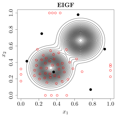
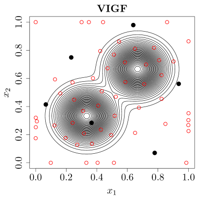
Figure 1: The sampling behaviour of EIGF (left) and VIGF (right) on a 2-dimensional problem which is a sum of two Gaussian functions. The black dots represent the initial design locations and red circles are the samples selected adaptively. EIGF takes many samples around the optimum $(1/3,1/3)^{\top}$. VIGF has a more global search due to the interaction between the exploration and exploitation components.

Extension to batch mode

In a batch mode sampling, a set of inputs are chosen for evaluation at each iteration. This can save the user time when parallel computing is available. Here, we propose the batch version of the VIGF criterion, called pseudo VIGF (PVIGF). It is obtained by multiplying VIGF by a repulsion/influence function, first introduced in [62] for batch Bayesian optimisation. The repulsion function (RF) is defined as

$$RF(\mathbf{x};\mathbf{x}_{u})=1-\mathbb{C}\text{orr}\left(Z_{n}(\mathbf{x}),Z_{n}(\mathbf{x}_{u})\right),$$ (12)

with $\mathbf{x}_{u}$ being an updating point. The RF function is zero at $\mathbf{x}_{u}$ and tends to one as $\lVert\mathbf{x}-\mathbf{x}_{u}\rVert\to\infty$. With the RF function one can add new design locations (as updating points) to the current DoE without evaluating the expensive function $f$. This is illustrated in Figure 2 where the left panel shows a GP fitted to five design points (black dots), and the corresponding VIGF criterion (right scale). In the right panel, the new location $x_{6}$ (blue circle) at which VIGF is maximum is added to the existing design without evaluating $f$ there. PVIGF (dashed red) is obtained by multiplying $VIGF(x)$ by $RF(x;x_{6})$ (dash-dotted green). The pseudocode of the batch mode sampling is presented in Algorithm 2 where $q>1$ locations are added to $\mathbf{X}_{n}$ at each iteration.

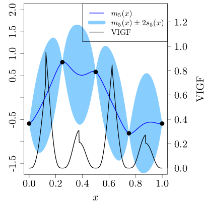
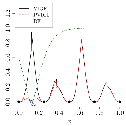
Figure 2: Left: A GP fitted to the five training data (black dots), and the corresponding VIGF function (right scale). Right: PVIGF (dashed red) is obtained by multiplying VIGF by the RF function (dash-dotted green) with the updating point $x_{6}$ (blue circle).

Algorithm 2 Choosing a batch of $q>1$ locations at each iteration

Input: GP $Z_{n}(\mathbf{x})$ which is constructed based on $\mathcal{A}=\{\mathbf{X}_{n},\mathbf{y}_{n}\}$

1:  Create $\text{VIGF}(\mathbf{x})$ using Equation (10)

2:  Compute $\mathbf{x}_{n+1}=\underset{\mathbf{x}\in\mathcal{D}}{\arg\!\max}\leavevmode\nobreak\ VIGF(\mathbf{x})$

3:  $PVIGF(\mathbf{x})=RF(\mathbf{x};\mathbf{x}_{n+1})VIGF(\mathbf{x})$

4:  for $j=2$ to $q$ do

5:     Compute $\mathbf{x}_{n+j}=\underset{\mathbf{x}\in\mathcal{D}}{\arg\!\max}\leavevmode\nobreak\ PVIGF(\mathbf{x})$

6:     $PVIGF(\mathbf{x})=RF(\mathbf{x};\mathbf{x}_{n+j})PVIGF(\mathbf{x})$

7:  end for

Output: $\mathbf{x}_{n+1},\mathbf{x}_{n+2},\ldots,\mathbf{x}_{n+q}$

Extension to multi-fidelity modelling

Now, we extend the proposed adaptive DoE to the two-level fidelity case in which a lower fidelity model contributes to the prediction of the high-fidelity simulator $f$. We tackle this problem by adapting the variable-fidelity method introduced in [63] relying on the HK model. The advantage of this approach is that the uncertainty due to the lack of a low-fidelity observation is analytically available, which may not be easily attainable in other approaches. It is shown that the predictive variance of the HK emulator associated with the lack of a low-fidelity sample at $\mathbf{x}\in\mathcal{D}$ is equal to $\beta\tilde{s}^{2}_{N}(\mathbf{x})$ [63]. Hence, the prediction uncertainty of the HK model can be expressed as a function of both the input values and the fidelity level as below

$$s^{2}_{n,HK}(\mathbf{x},L)=\begin{cases}\beta^{2}\tilde{s}^{2}_{N}(\mathbf{x})&\text{if }L=1\\ s^{2}_{n,HK}(\mathbf{x})&\text{if }L=2.\end{cases}$$ (13)

Here, $L$ indicates the fidelity level with $L=1$ for the low-fidelity model and $L=2$ for the high-fidelity one. In this setting, the prediction of the HK model and the improvement function at any point $\mathbf{x}$ are

$$Z_{n,HK}(\mathbf{x},L)\sim\mathcal{N}\left(m_{n,HK}(\mathbf{x}),s^{2}_{n,HK}(\mathbf{x},L)\right),$$ (14)

$$\mathcal{I}_{HK}(\mathbf{x},L)=\left(Z_{n,HK}(\mathbf{x},L)-f(\mathbf{x}_{i}^{*})\right)^{2},\quad L=1,2.$$ (15)

Note that $\mathcal{I}_{HK}(\mathbf{x},L)$ is a measure of the distance between $Z_{n,HK}(\mathbf{x},L)$ and the high-fidelity model output at $\mathbf{x}_{i}^{*}$, i.e., the closest design location to $\mathbf{x}$.

Now, the adaptive sampling criteria EIGF and VIGF can be easily extended to the two-level fidelity case. The new criteria, denoted by $EIGF_{HK}$ and $VIGF_{HK}$, are obtained if $m_{n}(\mathbf{x})$ and $s^{2}_{n}(\mathbf{x})$ in Equations (10) and (11) are replaced with $m_{n,HK}(\mathbf{x})$ (Equation (5)) and $s^{2}_{n,HK}(\mathbf{x},L)$ (Equation (13)), respectively. For example, $VIGF_{HK}$ takes the following form

$$VIGF_{HK}(\mathbf{x},L)=4s^{2}_{n,HK}\left(\mathbf{x},L\right)\left(m_{n,HK}(\mathbf{x})-f(\mathbf{x}_{i}^{*})\right)^{2}+2s^{4}_{n,HK}\left(\mathbf{x},L\right).$$ (16)

Note that the MSE criterion in a two-level fidelity model (denoted by $MSE_{HK}$) is expressed by Equation (13). The next sample point ($\mathbf{x}_{n+1}$) and its fidelity level ($L^{\ast}$) using the $VIGF_{HK}$ criterion are determined by solving the following optimisation problem

$$\mathbf{x}_{n+1},L^{\ast}=\underset{\mathbf{x}\in\mathcal{D},\,L=1,2}{\arg\!\max}\leavevmode\nobreak\ VIGF_{HK}(\mathbf{x},L),$$ (17)

given that we need to identify the location and fidelity level simultaneously. The same rule applies to $EIGF_{HK}$ and $MSE_{HK}$ when they are employed in a two-level adaptive sampling scheme.

4 Numerical experiments

The results of numerical experiments are presented in this section. The applicability of the proposed method is compared with several sampling schemes in both single and two-level fidelity cases on a suite of frequently used analytical test functions. The details are provided below.

4.1 Test functions and experimental setup

Our proposed adaptive DoE is applied to eight benchmark problems which serve as the ground truth models. They are summarised in Table 1 and their analytical expression is given in Appendix A. The functions $f_{1}-f_{6}$ are defined on the hypercube $[0,1]^{d}$. The problems $f_{7}$ and $f_{8}$ are physical models; the former simulates the midpoint voltage of an OTL push-pull circuit and the latter computes the cycle time of a piston within a cylinder. The functions are classified into two groups according to their dimensionality: small-scale ($1\leq d\leq 4$) and medium-scale ($5\leq d\leq 8$) [31]. In order to assess the accuracy of the emulator, we use the normalised root mean squared error (NRMSE) criterion

$$NRMSE=\frac{\sqrt{\frac{1}{n_{t}}\sum_{t=1}^{n_{t}}\left(m_{n}(\mathbf{x}_{t})-f(\mathbf{x}_{t})\right)^{2}}}{\underset{t=1:n_{t}}{\max}\,f(\mathbf{x}_{t})-\underset{t=1:n_{t}}{\min}\,f(\mathbf{x}_{t})},$$ (18)

wherein $\{\left(\mathbf{x}_{t},f(\mathbf{x}_{t})\right)\}_{t=1}^{t=n_{t}}$ is the test data set. In our experiments, $n_{t}=3000$ and the test points are spread across the domain uniformly. The total number of function evaluations is set to $30d$ and the size of initial design is $3d$.

Table 1: Summary of benchmark functions

	Function name	Dimension ($d$)	Scale
$f_{1}$	Franke [19]	2	Small
$f_{2}$	Dette & Pepelyshev (curved) [10]	3	Small
$f_{3}$	Hartmann [24]	3	Small
$f_{4}$	Park [60]	4	Small
$f_{5}$	Friedman [14]	5	Medium
$f_{6}$	Gramacy & Lee [18]	6	Medium
$f_{7}$	Output transformerless (OTL) circuit [5]	6	Medium
$f_{8}$	Piston simulation [5]	7	Medium

To construct GPs, the R package DiceKriging [50] is employed. The covariance kernel is Matérn $3/2$ and the unknown parameters are estimated by maximum likelihood. The Matérn covariance function is a popular choice in the computer experiments literature [6, 17]. The optimisation of the adaptive design criteria is performed via the R package DEoptim [45] which implements the differential evolution algorithm [58]. For each function, the sequential sampling methods are run with ten different initial space-filling designs. Thus, we have ten sets of NRMSE for each sampling strategy. The LHS designs are generated using the maximinESE_LHS function implemented in the R package DiceDesign [11]. This function employs a stochastic optimisation technique to produce an LHS design based on the maximin criterion.

4.2 Results and discussion

The results of our numerical experiments are illustrated in Figures 3 (small-scale) and 4 (medium-scale). Each curve represents the median of ten NRMSEs. The performance of VIGF (black) is compared with a number of adaptive sampling methods, i.e., EIGF (red), ES-LOO (orange), MSE (blue), MICE (green). In addition, the NRMSE based on the one-shot LHS design (cyan) is computed for all sample sizes $3d$, $4d,\ldots,30d$. The LHS design is also repeated ten times.

We observe that the design strategy proposed in this paper outperforms the other approaches in emulating the functions $f_{2},f_{4},f_{5},f_{6}$, and $f_{8}$, and its performance is comparable in the remaining cases ($f_{1}$, $f_{3}$, and $f_{7}$). This is due to the ability of VIGF to explore the input space while focusing on interesting regions. The EIGF method is the best algorithm on $f_{5}$ and $f_{7}$, however, its capability in emulating the multimodal functions $f_{1},f_{3}$, and $f_{6}$ is not favourable. It is highly likely that the EIGF criterion gets stuck in an optimum as discussed in Section 3. The method based on ES-LOO is never the winning algorithm, its accuracy results are promising yet except for $f_{4}$. The MSE criterion shows a good capability to predict small-scale problems as it tends to fill the space in a uniform manner, see below for further discussion. However, this is not the case for the medium (and possibly high) dimensional problems where the MSE measure tends to take more samples on the boundaries. The MICE algorithm performs poorly in all the cases due to its implementation on a discrete representation. The performance of the LHS design is comparable to the adaptive sampling approaches in most cases except the physical models, i.e., $f_{7}$ and $f_{8}$. The main disadvantage of the one-shot LHS design is that it can waste computational resources due to under/oversampling. We have also applied PVIGF with $q=4$ to the eight benchmark functions. It is found that PVIGF has a similar performance to VIGF. The results are presented in Figure 5.

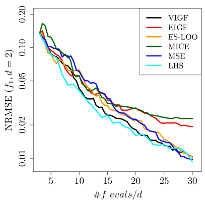
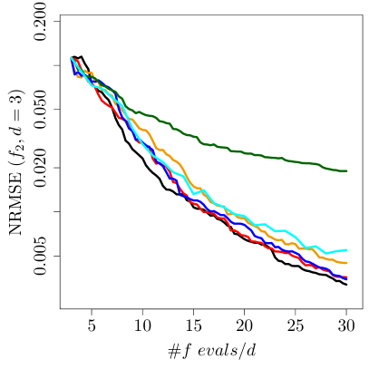
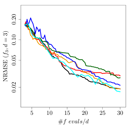
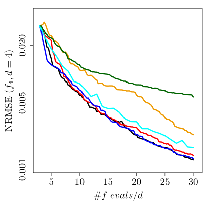
Figure 3: Accuracy results for the small-scale problems, i.e., $1\leq d\leq 4$. Each method generates ten prediction using ten different initial DoE. Every curve represents the median of ten NRMSEs obtained by VIGF (black), EIGF (red), ES-LOO (orange), MSE (blue), MICE (green), and the one-shot LHS design (cyan). For the latter, the NRMSE is computed for all sample sizes $3d$, $4d,\ldots,30d$. The $x$-axis shows the number of function calls divided by the problem dimensionality. The $y$-axis is on a logarithmic scale.

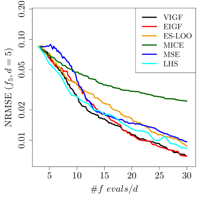
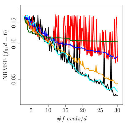
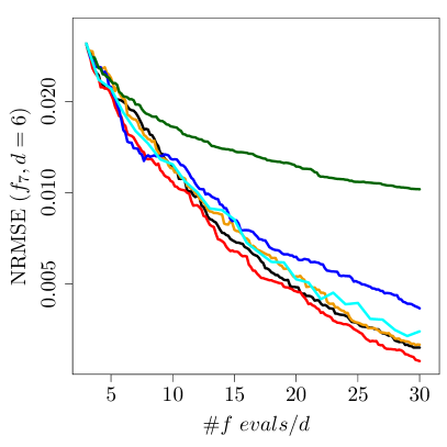
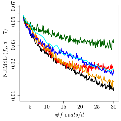
Figure 4: Accuracy results for the medium-scale problems, i.e., $5\leq d\leq 8$. Each curve is the median of ten RMSEs associated with the design based on VIGF (black), EIGF (red), ES-LOO (orange), MSE (blue), MICE (green), and the one-shot LHS design (cyan).

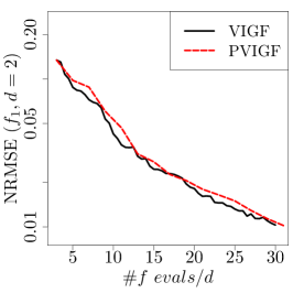
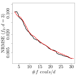
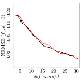
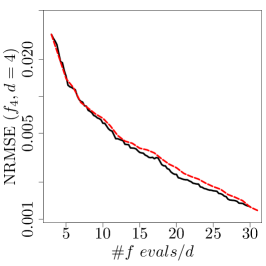
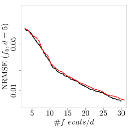
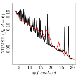
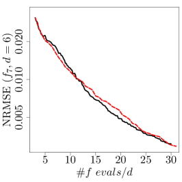
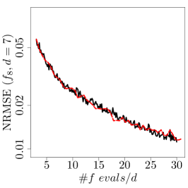
Figure 5: Accuracy results of VIGF (black) and PVIGF (red dashed) with $q=4$. As can be seen, VIGF and its batch version have similar performances. The advantage of the batch mode adaptive sampling is that it can save the user time when parallel computing is available.

The sampling behaviour of the above methods is further investigated using the discrepancy criterion [13, 12]. This function assesses the uniformity of a design by measuring how the empirical distribution of the points in the design deviates from the uniform distribution. The $\mathbb{L}^{2}$-discrepancy of a set $\mathbf{X}_{N^{\ast}}\subset[0,1]^{d}$ consisting of $N^{\ast}$ points is given by

$$D_{2}\left(\mathbf{X}_{N^{\ast}}\right)=\left[\int_{[0,1]^{d}}\left\lvert\frac{A\left(\mathbf{X}_{N^{\ast}},J_{\mathbf{x}}\right)}{N^{\ast}}-\text{Volume}\left(J_{\mathbf{x}}\right)\right\rvert^{2}\,d\mathbf{x}\right]^{1/2},$$ (19)

in which $J_{\mathbf{x}}$ denotes the interval $[0,\mathbf{x})=[0,x_{1})\times[0,x_{2})\times\ldots\times[0,x_{d})$, and $A\left(\mathbf{X}_{N^{\ast}},J_{\mathbf{x}}\right)$ returns the number of points of $\mathbf{X}_{N^{\ast}}$ falling in $J_{\mathbf{x}}$ [35].

We have computed the $\mathbb{L}^{2}$-discrepancy for all the sampling strategies used in this study. Figures 6 (small-scale) and 7 (medium-scale) display the box plot of the discrepancy results. As expected, the discrepancy of the LHS design is close to zero with a small variance. The method based on VIGF has neither the lowest nor highest discrepancy among the adaptive sampling approaches. This is due to the characteristic of VIGF that tends to fill the space with a focus on interesting regions. The discrepancy of PVIGF is close to that of VIGF. The discrepancy associated with the EIGF criterion is large in the problems $f_{1},f_{3}$, and $f_{6}$ where this criterion performs poorly. This can be explained by the tendency of EIGF towards local exploitation in those functions. It is observed that the design produced by the MICE algorithm has the smallest discrepancy after the LHS method. The discrepancy of MSE is significantly larger in the medium-scale functions than small-scale ones. The reason is that in the medium-scale functions many points are selected on their boundaries where the GP predictive variance is enormous.

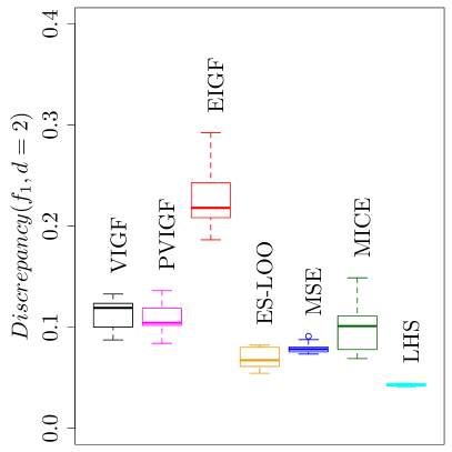
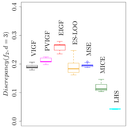
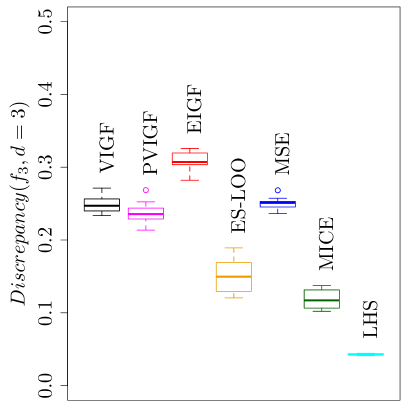
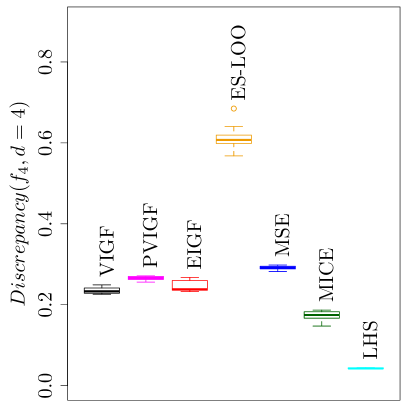
Figure 6: The box plot of the $\mathbb{L}^{2}$-discrepancy criterion for the designs obtained by VIGF (black), PVIGF (magenta), EIGF (red), ES-LOO (orange), MSE (blue), MICE (green), and LHS (cyan). The discrepancy measures how a given distribution of points differs from the uniform distribution. Accordingly, the LHS design has a very low discrepancy.

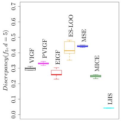
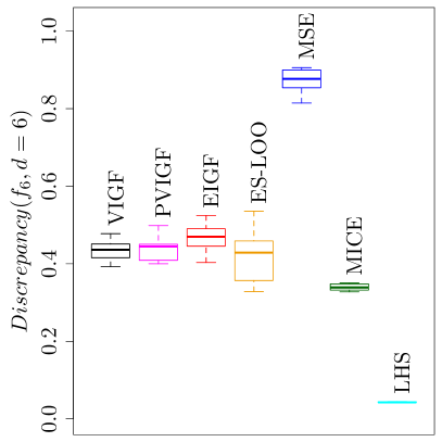
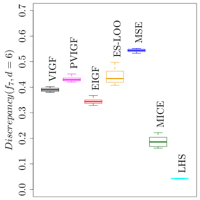
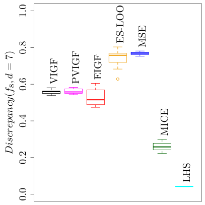
Figure 7: The box plot of the $\mathbb{L}^{2}$-discrepancy criterion for the methods based on VIGF (black), PVIGF (magenta), EIGF (red), ES-LOO (orange), MSE (blue), MICE (green), and LHS (cyan). The sampling scheme based on MSE leads to a large discrepancy in the medium-scale problems as many points are samples on their boundaries.

4.3 Two-level fidelity results

We assess the prediction capability of the proposed $VIGF_{HK}$ algorithm in the two-level fidelity case and compare the results with $EIGF_{HK}$ and $MSE_{HK}$. To do this, we consider four test examples that are commonly used as benchmark functions in multi-fidelity simulation studies. For example, one of them is the Borehole model [60] which is an eight-dimensional problem and simulates water flow through a borehole. The analytical expressions and the coarse version of the benchmark examples are given in Appendix B. The size of initial design to emulate $f$ and $\tilde{f}$ is $3d$ and $10d$, respectively. These points are generated based on LHS design in the same way as the single-fidelity case. A larger initial DoE is considered for $\tilde{f}$ given that it is computationally less demanding. We continue the sampling procedure until the total number of evaluations to $f$ and $\tilde{f}$ reaches $27d$. This makes our results consistent with the single-fidelity framework presented in Section 4.2.

Figure 8 shows the performance of the $VIGF_{HK}$ (black), $EIGF_{HK}$ (red), and $MSE_{HK}$ (blue) methods on the four test functions. Each curve represents the median of ten NRMSEs obtained using ten different initial DoE. Here, NRMSE is a measure of the distance between the emulator and high-fidelity function $f$. As can be seen, $VIGF_{HK}$ is the winning algorithm in general; it has a superior performance over $EIGF_{HK}$ in all cases. The accuracy obtained by $VIGF_{HK}$ and $MSE_{HK}$ is comparable on test functions $f_{4}$ and $f_{10}$. However, $VIGF_{HK}$ works better on $f_{9}$ and $f_{11}$.

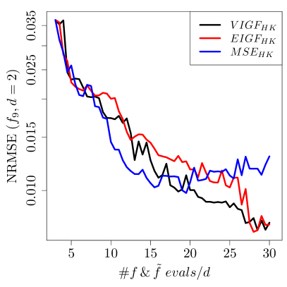
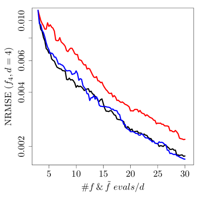
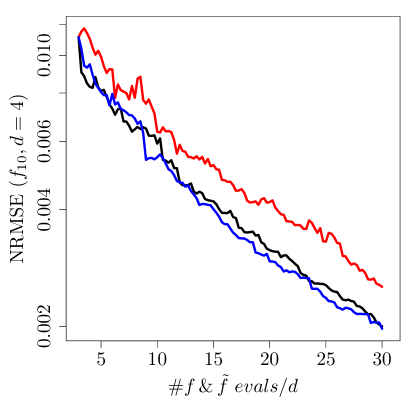
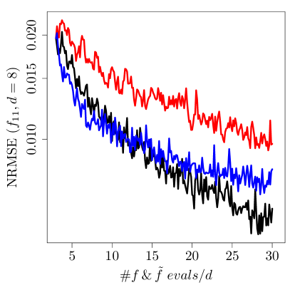
Figure 8: Accuracy results associated with $VIGF_{HK}$ (black), $EIGF_{HK}$ (red), and $MSE_{HK}$ (blue). Each curve is the median of ten NRMSEs. The $x$-axis represents the total number of evaluations to $f$ and $\tilde{f}$ divided by the problem dimension. The $y$-axis is on a logarithmic scale.

5 Conclusions

This paper presents a simple, yet effective GP-based adaptive sampling algorithm for predicting the output of computationally expensive computer codes. The method selects a new sample and add it to the current design $\mathbf{X}_{n}$ sequentially to improve the emulator using VIGF. This criterion is the variance of an improvement function defined at any $\mathbf{x}\in\mathcal{D}$ as the square of the difference between the fitted GP emulator and the model output at the nearest site in $\mathbf{X}_{n}$. The proposed selection criterion tends to fill the domain with a focus on “interesting” regions, where the model output changes drastically. Such property is due to an efficient trade-off between exploration and exploitation. We suggested the batch mode of VIGF by multiplying it by the repulsion function relying on the GP correlation function. Moreover, we proposed the extension of VIGF (and also EIGF and MSE) to the two-level fidelity case where in addition to the high-fidelity simulator, we have access to a coarse model which is cheap-to-evaluate. This is performed via the hierarchical kriging methodology. The performance of our method is evaluated on several commonly used benchmark functions and the accuracy results are compared with a few sampling strategies. We observed that our algorithm generally outperforms the other approaches in emulating the test cases.

Appendix A Test functions (single-fidelity)

1. $f_{1}(\mathbf{x})=0.75\exp\left(-\frac{(9x_{1}-2)^{2}}{4}-\frac{(9x_{2}-2)^{2}}{4}\right)+0.75\exp\left(-\frac{(9x_{1}+1)^{2}}{49}-\frac{9x_{2}+1)}{10}\right)\newline +0.5\exp\left(-\frac{(9x_{1}-7)^{2}}{4}-\frac{(9x_{2}-3)^{2}}{4}\right)-0.2\exp\left(-(9x_{1}-4)^{2}-(9x_{2}-7)^{2}\right)$

2. $f_{2}(\mathbf{x})=4\left(x_{1}-2+8x_{2}-8x_{2}^{2}\right)^{2}+\left(3-4x_{2}\right)^{2}+16\sqrt{x_{3}+1}\left(2x_{3}-1\right)^{2}.$

3. $f_{3}(\mathbf{x})=-\sum_{i=1}^{4}\boldsymbol{\alpha}_{i}\exp\left(\sum_{j=1}^{3}\mathbf{A}_{ij}\left(x_{j}-\mathbf{P}_{ij}\right)^{2}\right)$ where $\boldsymbol{\alpha}=(1,1.2,3,3.2)^{\top}$,
   

   $$\mathbf{A}=\begin{bmatrix}3&10&30\\ 0.1&10&35\\ 3&10&30\\ 0.1&10&35\end{bmatrix},\quad\mathbf{P}=10^{-4}\begin{bmatrix}3689&1170&2673\\ 4699&4387&7470\\ 1091&8732&5547\\ 381&5743&8828\end{bmatrix}$$

4. $f_{4}(\mathbf{x})=\frac{x_{1}}{2}\left(\sqrt{1+(x_{2}+x_{3}^{2})\frac{x_{4}}{x_{1}^{2}}}-1\right)+(x_{1}+3x_{4})\exp\left(1+\sin(x_{3})\right)$

5. $f_{5}(\mathbf{x})=10\sin(\pi x_{1}x_{2})+20(x_{3}-0.5)^{2}+10x_{4}+5x_{5}$

6. $f_{6}(\mathbf{x})=\exp\left(\sin\left([0.9(x_{1}+0.48))]^{10}\right)\right)+x_{2}x_{3}+x_{4}$

7. $f_{7}(\mathbf{x})=\frac{(V_{b}+0.74)x_{6}(x_{5}+9)}{x_{6}(x_{5}+9)+x_{3}}+\frac{11.35x_{3}}{x_{6}(x_{5}+9)+x_{3}}+\frac{0.74x_{3}x_{6}(x_{5}+9)}{(x_{6}(x_{5}+9)+x_{3})x_{4}}$ where $V_{b}=\frac{12x_{2}}{x_{1}+x_{2}}$ with:

   • $x_{1}\in\left[50,150\right]$ is the resistance $b_{1}$ (K-Ohms)

   • $x_{2}\in\left[25,70\right]$ is the resistance $b_{2}$ (K-Ohm)

   • $x_{3}\in\left[0.5,3\right]$ is the resistance $f$ (K-Ohms)

   • $x_{4}\in\left[1.2,2.5\right]$ is the resistance $c_{1}$ (K-Ohms)

   • $x_{5}\in\left[0.25,1.2\right]$ is the resistance $c_{2}$ (K-Ohms)

   • $x_{6}\in\left[50,300\right]$ is the current gain $c_{1}$ (amperes)

8. $f_{8}(\mathbf{x})=2\pi\sqrt{\frac{x_{1}}{x_{4}+x_{2}^{2}\frac{x_{5}x_{3}x_{6}}{x_{7}V^{2}}}}$ where $V=\frac{x_{2}}{2x_{4}}\left(\sqrt{A^{2}+4x_{4}\frac{x_{5}x_{3}}{x_{7}}x_{6}}-A\right)$ and
   $A=x_{5}x_{2}+19.62x_{1}-\frac{x_{4}x_{3}}{x_{2}}$ with:

   • $x_{1}\in\left[30,60\right]$ is the piston weight (kg)

   • $x_{2}\in\left[0.005,0.020\right]$ is the piston surface area ($m^{2}$)

   • $x_{3}\in\left[0.002,0.010\right]$ is the initial gas volume ($m^{3}$)

   • $x_{4}\in\left[1000,5000\right]$ is the spring coefficient ($N/m$)

   • $x_{5}\in\left[90000,110000\right]$ is the atmospheric pressure ($N/m^{2}$)

   • $x_{6}\in\left[290,296\right]$ is the ambient temperature (K)

   • $x_{7}\in\left[340,360\right]$ is the filling gas temperature (K)

Appendix B Test functions (two-level fidelity)

1. $\tilde{f}_{4}(\mathbf{x})=\left(1+\frac{\sin(x_{1})}{10}\right)f_{4}(\mathbf{x})-2x_{1}+x_{2}^{2}+x_{3}^{2}+0.5$

2. $f_{9}(\mathbf{x})=\left(1-\exp\left(-\frac{1}{2x_{2}}\right)\right)\frac{2300x_{1}^{3}+1900x_{1}^{2}+2092x_{1}+60}{100x_{1}^{3}+500x_{1}^{2}+4x_{1}+20}$

3. $\tilde{f}_{9}(\mathbf{x})=\frac{1}{4}\left[f_{9}(x_{1}+0.05,x_{2}+0.05)+f_{9}(x_{1}+0.05,\max(0,x_{2}-0.05))\right]\newline +\frac{1}{4}\left[f_{9}(x_{1}-0.05,x_{2}+0.05)+f_{9}(x_{1}-0.05,\max(0,x_{2}-0.05))\right]$

4. $f_{10}(\mathbf{x})=\frac{2}{3}\exp(x_{1}+x_{2})-x_{4}\sin(x_{3})+x_{3}$

5. $\tilde{f}_{10}(\mathbf{x})=1.2f_{10}(\mathbf{x})-1$

6. $f_{11}(\mathbf{x})=\frac{2\pi x_{1}(x_{2}-x_{3})}{\ln(x_{4}/x_{5})\left(1+\frac{2x_{6}x_{1}}{\ln(x_{4}/x_{5})x_{5}^{2}x_{7}}+\frac{x_{1}}{x_{8}}\right)}$ with:

   • $x_{1}\in\left[63070,115600\right]$ is transmissivity of upper aquifer ($m^{2}/yr$)

   • $x_{2}\in\left[990,1110\right]$ is potentiometric head of upper aquifer ($m$)

   • $x_{3}\in\left[700,820\right]$ is potentiometric head of lower aquifer ($m$)

   • $x_{4}\in\left[100,50000\right]$ is radius of influence ($m$)

   • $x_{5}\in\left[0.05,0.15\right]$ is radius of borehole ($m$)

   • $x_{6}\in\left[1120,1680\right]$ is length of borehole ($m$)

   • $x_{7}\in\left[9855,12045\right]$ is hydraulic conductivity of borehole ($m/yr$)

   • $x_{8}\in\left[63.1,116\right]$ is transmissivity of lower aquifer ($m^{2}/yr$)

7. $\tilde{f}_{11}(\mathbf{x})=\frac{5x_{1}(x_{2}-x_{3})}{\ln(x_{4}/x_{5})\left(1.5+\frac{2x_{6}x_{1}}{\ln(x_{4}/x_{5})x_{5}^{2}x_{7}}+\frac{x_{1}}{x_{8}}\right)}$

References

- [1] Imad Abdallah, Christos Lataniotis, and Bruno Sudret. Parametric hierarchical kriging for multi-fidelity aero-servo-elastic simulators-application to extreme loads on wind turbines. Probabilistic Engineering Mechanics, 55:67–77, 2019.
- [2] Reza Alizadeh, Janet K. Allen, and Farrokh Mistree. Managing computational complexity using surrogate models: a critical review. Research in Engineering Design, 31(3):275–298, 2020.
- [3] V. Aute, K. Saleh, O. Abdelaziz, S. Azarm, and R. Radermacher. Cross-validation based single response adaptive design of experiments for kriging metamodeling of deterministic computer simulations. Structural and Multidisciplinary Optimization, 48(3):581–605, 2013.
- [4] J. Beck and S. Guillas. Sequential design with mutual information for computer experiments (MICE): emulation of a tsunami model. SIAM/ASA Journal on Uncertainty Quantification, 4(1):739–766, 2016.
- [5] Einat Neumann Ben-Ari and David M. Steinberg. Modeling data from computer experiments: An empirical comparison of kriging with mars and projection pursuit regression. Quality Engineering, 19(4):327–338, 2007.
- [6] Mickaël Binois, Jiangeng Huang, Robert B. Gramacy, and Mike Ludkovski. Replication or exploration? sequential design for stochastic simulation experiments. Technometrics, 61(1):7–23, 2019.
- [7] G. E. P. Box and J. S. Hunter. The 2k-p fractional factorial designs part ii. Technometrics, 3(4):449–458, 1961.
- [8] Kathryn Chaloner and Isabella Verdinelli. Bayesian experimental design: A review. Statistical Science, 10(3):273–304, 1995.
- [9] D. Austin Cole, Robert B. Gramacy, James E. Warner, Geoffrey F. Bomarito, Patrick E. Leser, and William P. Leser. Entropy-based adaptive design for contour finding and estimating reliability. Journal of Quality Technology, pages 1–18, 2022.
- [10] Holger Dette and Andrey Pepelyshev. Generalized Latin hypercube design for computer experiments. Technometrics, 52(4):421–429, 2010.
- [11] Delphine Dupuy, Céline Helbert, and Jessica Franco. DiceDesign and DiceEval: two R packages for design and analysis of computer experiments. Journal of Statistical Software, 65(11):1–38, 2015.
- [12] Kai-Tai Fang and Rahul Mukerjee. A connection between uniformity and aberration in regular fractions of two-level factorials. Biometrika, 87(1):193–198, 2000.
- [13] Kai-Tai Fang, Yuan Wang, and Peter M. Bentler. Some applications of number-theoretic methods in statistics. Statistical Science, 9(3):416–428, 1994.
- [14] Jerome H. Friedman. Multivariate adaptive regression splines. The Annals of Statistics, 19(1):1–67, 1991.
- [15] Jan N. Fuhg, Amélie Fau, and Udo Nackenhorst. State-of-the-art and comparative review of adaptive sampling methods for kriging. Archives of Computational Methods in Engineering, 28(4):2689–2747, 2021.
- [16] Sushant S. Garud, Iftekhar A. Karimi, and Markus Kraft. Design of computer experiments: a review. Computers & Chemical Engineering, 106:71–95, 2017. ESCAPE-26.
- [17] Robert B. Gramacy. Surrogates: Gaussian Process Modeling, Design and Optimization for the Applied Sciences. Chapman Hall/CRC, Boca Raton, Florida, 2020. http://bobby.gramacy.com/surrogates/.
- [18] Robert B. Gramacy and Herbert K. H. Lee. Adaptive design and analysis of supercomputer experiments. Technometrics, 51(2):130–145, 2009.
- [19] Ben Haaland and Peter Z. G. Qian. Accurate emulators for large-scale computer experiments. The Annals of Statistics, 39(6):2974–3002, 2011.
- [20] J. H. Halton. On the efficiency of certain quasi-random sequences of points in evaluating multi-dimensional integrals. Numerische Mathematik, 2(1):84–90, 1960.
- [21] Zhong-Hua Han and Stefan Görtz. Hierarchical kriging model for variable-fidelity surrogate modeling. AIAA Journal, 50(9):1885–1896, 2012.
- [22] Philipp Hennig and Christian J. Schuler. Entropy search for information-efficient global optimization. Journal of Machine Learning Research, 13:1809–1837, 2012.
- [23] José Miguel Henrández-Lobato, Matthew W. Hoffman, and Zoubin Ghahramani. Predictive entropy search for efficient global optimization of black-box functions. In Proceedings of the 27th International Conference on Neural Information Processing Systems, NIPS’14, pages 918–926. MIT Press, 2014.
- [24] Momin Jamil and Xin-She Yang. A literature survey of benchmark functions for global optimization problems. International Journal of Mathematical Modelling and Numerical Optimisation, 4(2):150–194, 2013.
- [25] Ping Jiang, Leshi Shu, Qi Zhou, Hui Zhou, Xinyu Shao, and Junnan Xu. A novel sequential exploration-exploitation sampling strategy for global metamodeling. IFAC-PapersOnLine, 48(28):532–537, 2015.
- [26] Ruichen Jin, Wei Chen, and Agus Sudjianto. On sequential sampling for global metamodeling in engineering design. In Design Engineering Technical Conferences And Computers and Information in Engineering, volume 2, pages 539–548, 2002.
- [27] M.E. Johnson, L.M. Moore, and D. Ylvisaker. Minimax and maximin distance designs. Journal of Statistical Planning and Inference, 26(2):131–148, 1990.
- [28] Crombecq Karel, Dirk Gorissen, Dirk Deschrijver, and Tom Dhaene. A novel hybrid sequential design strategy for global surrogate modeling of computer experiments. SIAM Journal on Scientific Computing, 33(4):1948–1974, 2011.
- [29] Elizabeth J. Kendon, Nigel M. Roberts, Hayley J. Fowler, Malcolm J. Roberts, Steven C. Chan, and Catherine A. Senior. Heavier summer downpours with climate change revealed by weather forecast resolution model. Nature Climate Change, 4(7):570–576, 2014.
- [30] M. C. Kennedy and A. O’Hagan. Predicting the output from a complex computer code when fast approximations are available. Biometrika, 87(1):1–13, 2000.
- [31] Mohammed Reza Kianifar and Felician Campean. Performance evaluation of metamodelling methods for engineering problems: towards a practitioner guide. Structural and Multidisciplinary Optimization, 61(1):159–186, 2020.
- [32] Andreas Krause, Ajit Singh, and Carlos Guestrin. Near-optimal sensor placements in Gaussian processes: Theory, efficient algorithms and empirical studies. Journal of Machine Learning Research, 9:235–284, February 2008.
- [33] Chen Quin Lam. Sequential adaptive designs in computer experiments for response surface model fit. PhD thesis, Columbus, OH, USA, 2008. AAI3321369.
- [34] Genzi Li, Vikrant Aute, and Shapour Azarm. An accumulative error based adaptive design of experiments for offline metamodeling. Structural and Multidisciplinary Optimization, 40(1):137–157, 2009.
- [35] C. Devon Lin and Boxin Tang. Handbook of Design and Analysis of Experiments, chapter Latin hypercubes and space-filling designs. Chapman & Hall/CRC, London, 2015.
- [36] Haitao Liu, Yew-Soon Ong, and Jianfei Cai. A survey of adaptive sampling for global metamodeling in support of simulation-based complex engineering design. Structural and Multidisciplinary Optimization, 57(1):393–416, 2018.
- [37] Haitao Liu, Shengli Xu, Ying Ma, Xudong Chen, and Xiaofang Wang. An adaptive Bayesian sequential sampling approach for global metamodeling. Journal of Mechanical Design, 138(1), 2015.
- [38] A. Lopez-Perez, R. Sebastian, M. Izquierdo, R. Ruiz, M. Bishop, and J. M. Ferrero. Personalized cardiac computational models: from clinical data to simulation of infarct-related ventricular tachycardia. Frontiers in Physiology, 10, 2019.
- [39] Dan Maljovec, Bei Wang, Ana Kupresanin, Gardar Johannesson, Valerio Pascucci, and Peer-Timo Bremer. Adaptive sampling with topological scores. International Journal for Uncertainty Quantification, 3:119–141, 01 2013.
- [40] Sébastien Marmin, David Ginsbourger, Jean Baccou, and Jacques Liandrat. Warped Gaussian processes and derivative-based sequential designs for functions with heterogeneous variations. SIAM/ASA Journal on Uncertainty Quantification, 6(3):991–1018, 2018.
- [41] Alexandre Marques, Remi Lam, and Karen Willcox. Contour location via entropy reduction leveraging multiple information sources. In Advances in Neural Information Processing Systems, volume 31, pages 5222–5232. Curran Associates, Inc., 2018.
- [42] M. D. McKay, R. J. Beckman, and W. J. Conover. A comparison of three methods for selecting values of input variables in the analysis of output from a computer code. Technometrics, 21(2):239–245, 1979.
- [43] Hossein Mohammadi, Peter Challenor, Daniel Williamson, and Marc Goodfellow. Cross-validation–based adaptive sampling for Gaussian process models. SIAM/ASA Journal on Uncertainty Quantification, 10(1):294–316, 2022.
- [44] Mohammad A. Mohammadi and Ali Jafarian. CFD simulation to investigate hydrodynamics of oscillating flow in a beta-type Stirling engine. Energy, 153:287–300, 2018.
- [45] Katharine M. Mullen, David Ardia, David L. Gil, Donald Windover, and James Cline. DEoptim: an R package for global optimization by differential evolution. Journal of Statistical Software, Articles, 40(6):1–26, 2011.
- [46] Art B. Owen. Orthogonal arrays for computer experiments, integration and visualization. Statistica Sinica, 2(2):439–452, 1992.
- [47] Benjamin Peherstorfer, Karen Willcox, and Max Gunzburger. Survey of multifidelity methods in uncertainty propagation, inference, and optimization. SIAM Review, 60(3):550–591, 2018.
- [48] V. Picheny, D. Ginsbourger, O. Roustant, R. T. Haftka, and N. H. Kim. Adaptive designs of experiments for accurate approximation of a target region. Journal of Mechanical Design, 132(7):1–9, 2010.
- [49] Carl Edward Rasmussen and Christopher K. I. Williams. Gaussian processes for machine learning (adaptive computation and machine learning). The MIT Press, 2005.
- [50] Olivier Roustant, David Ginsbourger, and Yves Deville. DiceKriging, DiceOptim: two R packages for the analysis of computer experiments by kriging-based metamodeling and optimization. Journal of Statistical Software, 51(1):1–55, 2012.
- [51] Jerome Sacks, William J. Welch, Toby J. Mitchell, and Henry P. Wynn. Design and analysis of computer experiments. Statistical Science, 4(4):409–423, 1989.
- [52] Andrea Saltelli, Stefano Tarantola, Francesca Campolongo, and Marco Ratto. Sensitivity analysis in practice: A guide to assessing scientific models. Wiley, 2004.
- [53] T. J. Santner, Williams B., and Notz W. The Design and Analysis of Computer Experiments, Second Edition. Springer-Verlag, 2018.
- [54] Claude Elwood Shannon. A mathematical theory of communication. The Bell System Technical Journal, 27(3):379–423, 1948.
- [55] Razi Sheikholeslami and Saman Razavi. Progressive Latin hypercube sampling: an efficient approach for robust sampling-based analysis of environmental models. Environmental Modelling & Software, 93:109 – 126, 2017.
- [56] M. C. Shewry and H. P. Wynn. Maximum entropy sampling. Journal of Applied Statistics, 14(2):165–170, 1987.
- [57] I.M Sobol’. On the distribution of points in a cube and the approximate evaluation of integrals. USSR Computational Mathematics and Mathematical Physics, 7(4):86–112, 1967.
- [58] Rainer Storn and Kenneth Price. Differential evolution – a simple and efficient heuristic for global optimization over continuous spaces. Journal of Global Optimization, 11(4):341–359, 1997.
- [59] Georges Voronoi. Nouvelles applications des paramètres continus à la théorie des formes quadratiques. premier mémoire. sur quelques propriétès des formes quadratiques positives parfaites. Journal für die reine und angewandte Mathematik, 133:97–178, 1908.
- [60] Shifeng Xiong, Peter Z. G. Qian, and C. F. Jeff Wu. Sequential design and analysis of high-accuracy and low-accuracy computer codes. Technometrics, 55(1):37–46, 2013.
- [61] Shengli Xu, Haitao Liu, Xiaofang Wang, and Xiaomo Jiang. A robust error-pursuing sequential sampling approach for global metamodeling based on Voronoi diagram and cross validation. Journal of Mechanical Design, 136(7), 04 2014.
- [62] Dawei Zhan, Jiachang Qian, and Yuansheng Cheng. Pseudo expected improvement criterion for parallel EGO algorithm. Journal of Global Optimization, 68(3):641–662, 2017.
- [63] Yu Zhang, Zhong-Hua Han, and ke-shi Zhang. Variable-fidelity expected improvement method for efficient global optimization of expensive functions. Structural and Multidisciplinary Optimization, 58(4):1431–1451, 2018.