Ground state selection by magnon interactions in the fcc antiferromagnet

Abstract

We study the nearest-neighbor Heisenberg antiferromagnet on a face-centered cubic lattice with arbitrary spin $S$. The model exhibits degenerate classical ground states including two collinear structures AF1 and AF3 described by different propagation vectors that are prime candidates for the quantum ground state. We compute the energy for each of the two states as a function of $S$ using the spin-wave theory that includes magnon-magnon interaction in a self-consistent way and the numerical coupled cluster method. Our results unambiguously demonstrate that quantum fluctuations stabilize the AF1 state for realistic values of spin. Transition to the harmonic spin-wave result, which predicts the AF3 state, takes place only for $S\gtrsim 10$. We also study quantum renormalization of the magnon spectra for both states as a function of spin.

I Introduction

An antiferromagnet on a face-centered cubic lattice has attracted a longstanding theoretical interest [1, 2, 3, 4, 5, 6, 7, 8, 9, 10, 11, 12, 13, 14, 15, 16, 17, 18, 19, 20, 21, 22, 23, 24, 25, 26]. Early on, Anderson argued for an infinite degeneracy of the classical ground state for the nearest-neighbor Heisenberg model [1] making it the second such example after the celebrated triangular Ising antiferromagnet [27]. The interest in magnetic frustration on the face-centered cubic (fcc) network is fueled by an abundance of related materials, see [28] for survey of the early works and [29, 30, 31, 32, 33, 34, 35] for more recent studies.

The infinite degeneracy in the ground state can be lifted by additional interactions, for example, the second-neighbor exchange $J_{2}$ that is often present in the fcc materials [28]. The two collinear AF1 and AF3 spin structures stabilized, respectively, by weak negative or positive $J_{2}$ are shown in Fig. 1. The propagation vector of the AF1 magnetic structure is ${\bf Q}_{1}=(2\pi,0,0)$ or the two other wavevectors obtained by permutation of its components. The AF3 magnetic structure is described by ${\bf Q}_{3}=(2\pi,\pi,0)$ or other symmetry related vector in the Brillouin Zone (BZ). For the nearest-neighbor model ($J_{2}=0$) the two collinear states become degenerate together with an infinite number of incommensurate spin spirals described by wavevectors belonging to the line ${\bf Q}_{s}=(2\pi,q,0)$ that connects the AF1 and AF3 wavevectors.

The problem of a finite-temperature transition in an infinitely degenerate frustrated spin model as well as subsequent selection of a specific ground state structure by quantum fluctuations was formulated already in the early works [3, 4, 5]. The nonzero transition temperature for the nearest-neighbor Heisenberg fcc model was unambiguously demonstrated by classical Monte Carlo simulations [12, 16]. However, the question about its ground state for the quantum model has not been satisfactorily answered. The two main contenders are collinear AF1 and AF3 states since quantum effects, often called ‘order by disorder’, usually disfavor noncollinear spin arrangements [36, 37, 38, 39]. The exact-diagonalization study of the $J_{1}$–$J_{2}$ spin-1/2 fcc antiferromagnet in zero field [15] was performed on clusters up to $N=32$ sites, which is clearly insufficient to reach a conclusion about the type of a long-range order for $J_{2}=0$. In the recent article, three of us investigated this problem in the harmonic spin-wave approximation [25]. The energy difference between the AF1 and AF3 structures is found to be

$$\Delta E_{13}=E_{\rm AF1}-E_{\rm AF3}=0.00305(1)JS\,.$$ (1)

suggesting that the AF3 spin structure is the ground state. Still, $\Delta E_{13}$ remains very small and the above conclusion may be affected by the magnon-magnon interaction.

The $1/S$ spin-wave expansion works poorly for highly-frustrated antiferromagnets with lines of pseudo-Goldstone (zero-energy) modes in the harmonic spectra, see, e.g., [40]. Instead, in this work we perform a self-consistent spin-wave calculation, which corresponds to summation of an infinite sub-series of the $1/S$ diagrams. The magnon interaction renormalizes the bare excitation energies such that the accidental zero-energy magnons acquire finite quantum gaps. The ground-state energy correction obtained with the renormalized magnon spectrum is expected to be more reliable. In addition, we obtain the ground state energies numerically using the coupled-clusters method, which appears to be one of a few techniques suitable for numerical investigation of three-dimensional frustrated magnets. Both approaches agree that the AF1 state is the ground state of the Heisenberg fcc antiferromagnet for all physical values of spin $S\lesssim 10$. Furthermore, the absolute energy values are in good correspondence between the two approaches.

The paper is organized as follows. Section II describes the self-consistent spin-wave calculations. The general idea of the approach is outlined in Sec. IIA, whereas analytic results for the AF1 and AF3 states are provided in Secs. IIB and IIC, respectively. Details of the coupled cluster method (CCM) are presented in Sec. III. Our main results for the fcc antiferromagnet obtained by the two methods are included in Sec. IV, where we discuss the ground state properties as well as quantum renormalization of the magnon spectra. Sec. V is devoted to further discussion and conclusions. Appendices provide extra details on self-consistent calculations and spectrum renormalization for the AF3 state, Appen. A, and on the CCM extrapolation for $S=1/2$ and 1, Appen. B.

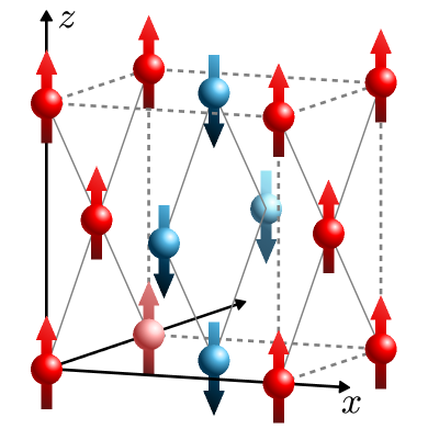
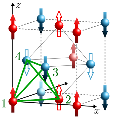
Figure 1: Collinear magnetic structures for the nearest-neighbor fcc antiferromagnet. Left: the two-sublattice AF1 state with ${\bf Q}_{1}=(2\pi,0,0)$. Right: the four-sublattice AF3 state with ${\bf Q}_{3}=(2\pi,\pi,0)$. Closed (open) spins correspond to two rotating sublattices described by $a$ ($b$) bosons (see the text).

II Spin-wave theory

II.1 Self-consistent approach

We use the self-consistent spin-wave theory to study quantum effects in the Heisenberg antiferromagnet on an fcc lattice with nearest-neighbor interactions between spins of length $S$:

$$\hat{\cal H}=J\sum_{\langle ij\rangle}{\bf S}_{i}\cdot{\bf S}_{j}\,.$$ (2)

One of the first formulations of the self-consistent approach was given by Takahashi in a study of a square-lattice antiferromagnet at finite temperatures [41]. Various extensions of the Takahashi’s work were subsequently applied to ordered and disordered quantum magnetic phases at zero and finite temperatures [42, 43, 44, 45, 46, 47, 48, 49, 50, 51, 52]. We outline details relevant for ordered magnetic states at $T=0$ below.

We use the Holstein-Primakoff representation of spin operators [53]

$$S^{-}=a^{\dagger}\,\sqrt{2S-a^{\dagger}a}\approx\sqrt{2S}a^{\dagger}\Bigl{(}1-\frac{a^{\dagger}a}{4S}\Bigr{)},$$

$$S^{+}=(S^{-})^{\dagger},\ \ S^{z}=S-a^{\dagger}a$$ (3)

applied in the local rotating frame associated with the average spin direction on each site. The bond Hamiltonian is, then, expressed via bosonic operators

$$\hat{\cal H}_{ij}=J{\bf S}_{i}\cdot{\bf S}_{j}\approx E_{ij}^{(0)}+\hat{\cal H}_{ij}^{(2)}+\hat{\cal H}_{ij}^{(4)}\,,$$ (4)

restricting expansion up to the fourth order terms.

For the nearest-neighbor fcc antiferromagnet we have to distinguish two types of bonds with antiparallel ($\uparrow\downarrow$) and parallel ($\uparrow\uparrow$) orientation of spins. In AF1 and AF3 structures every spin participates in eight $\uparrow\downarrow$ bonds and four $\uparrow\uparrow$ bonds giving them the same classical energy

$$E_{0}/N=-2JS^{2}\,.$$ (5)

The quadratic bond contributions are

$$\hat{\cal H}_{\uparrow\uparrow}^{(2)} = JS\bigl{(}a_{i}^{\dagger}a_{j}+a_{j}^{\dagger}a_{i}-a_{i}^{\dagger}a_{i}-a_{j}^{\dagger}a_{j}\bigr{)}\,,$$

$$\hat{\cal H}_{\uparrow\downarrow}^{(2)} = JS\bigl{(}a_{i}^{\dagger}a_{i}+a_{j}^{\dagger}a_{j}-a_{i}a_{j}-a_{i}^{\dagger}a_{j}^{\dagger}\bigr{)}\,.$$ (6)

The nonlinear quartic terms responsible for magnon-magnon interaction are expressed as

$$\hat{\cal H}_{\uparrow\uparrow}^{(4)} = J\Bigl{[}n_{i}n_{j}-\frac{1}{4}\bigl{(}a_{i}^{\dagger}n_{i}a_{j}+a_{i}^{\dagger}n_{j}a_{j}+\textrm{h.c.}\bigr{)}\Bigr{]}\,,$$

$$\hat{\cal H}_{\uparrow\downarrow}^{(4)} = J\Bigl{[}-n_{i}n_{j}+\frac{1}{4}\bigl{(}n_{i}a_{i}a_{j}+n_{j}a_{i}a_{j}+\textrm{h.c.}\bigr{)}\Bigr{]}\,.$$ (7)

where h.c. stands for the Hermitian conjugate terms and $n_{i}=a_{i}^{\dagger}a_{i}$ is the occupation number operator.

The harmonic or linear spin-wave theory amounts to keeping only quadratic terms in the boson Hamiltonian. Standard diagonalization of $\hat{\cal H}^{(2)}$ with the help of the Fourier and the Bogolyubov transformations yields the bare magnon energies. One can also compute the expectation values of various boson averages in the harmonic ground-state

$$n=\langle a_{i}^{\dagger}a_{i}\rangle\,,\ \ m_{ij}=\langle a_{i}^{\dagger}a_{j}\rangle\,,\ \ \Delta_{ij}=\langle a_{i}a_{j}\rangle\,.$$ (8)

Performing linear spin-wave calculations for a chosen state, it is straightforward to verify that the normal averages $m_{ij}$ are nonzero for bonds with parallel spins and vanish for all antiparallel pairs. The anomalous averages $\Delta_{ij}$ exhibit the opposite pattern: nonzero for $\uparrow\downarrow$ and zero for $\uparrow\uparrow$ spin pairs. These relations are imposed by conservation of the $z$-component of the total spin for a collinear antiferromagnet with continuous rotation symmetry about the sublattice direction. Thus, they hold beyond the harmonic approximation in all orders with respect to magnon-magnon interaction. Once the continuous rotations are absent, either at the level of a spin Hamiltonian or because of spin orientation, nonzero $m_{ij}$, $\Delta_{ij}$ appear for every bond.

The next step is to decompose the quartic Hamiltonian $\hat{\cal H}^{(4)}$ into quadratic terms using the standard Hartree-Fock decoupling with the mean-field averages defined by (8). Basically, this approximation implies that the magnon scattering process are neglected. Skipping straightforward intermediate steps and collecting all relevant contributions we obtain

$$\hat{\cal H}_{\uparrow\uparrow} \approx J\Bigl{[}S^{2}-(n-m_{ij})^{2}+(S-n+m_{ij})$$

$$\times (a_{i}^{\dagger}a_{j}+a_{j}^{\dagger}a_{i}-a_{i}^{\dagger}a_{i}-a_{j}^{\dagger}a_{j})\Bigr{]},$$

$$\hat{\cal H}_{\uparrow\downarrow} \approx J\Bigl{[}-S^{2}+\left(n-\Delta_{ij}\right)^{2}$$

$$+ (S-n+\Delta_{ij})(a_{i}^{\dagger}a_{i}+a_{j}^{\dagger}a_{j}-a_{i}a_{j}-a_{i}^{\dagger}a_{j}^{\dagger})\Bigr{]}.$$

At this point the mean-field averages are considered as independent parameters and the excitation spectrum is obtained by diagonalization of a new quadratic Hamiltonian $\hat{\cal H}^{(2)}_{\rm MF}$ obtained by summation of bond contributions (II.1). The system is finally closed by a self-consistency condition (8), where the averages are computed over a new renormalized ground state.

Once a solution of the self-consistent equations is obtained, the ground state energy can be expressed as

$$E_{\textrm{g.s.}} = E_{0}+\langle\hat{\cal H}^{(2)}+\hat{\cal H}^{(4)}\rangle$$

$$= J\sum_{\langle ij\rangle}^{\uparrow\uparrow}(S\!-\!n\!+\!m_{ij})^{2}-J\sum_{\langle ij\rangle}^{\uparrow\downarrow}(S\!-\!n\!+\!\Delta_{ij})^{2}.$$

In the following subsections we give explicit analytic results for the AF1 and the AF3 states of the fcc antiferromagnet.

II.2 AF1 state

The antiferromagnetic AF1 structure consists of two opposite magnetic sublattices which transform into each other under translation. As a result, the exchange bonds are characterized by only two mean-field averages: $m_{ij}=m$ and $\Delta_{ij}=\Delta$ for parallel and antiparallel pairs of spins, respectively. Choosing among three equivalent domains the state with ${\bf Q}_{1}=(2\pi,0,0)$, we introduce a single species of bosons in the rotating spin frame and obtain for the quadratic part of the mean-field Hamiltonian (II.1):

$$\hat{\cal H}^{(2)}_{MF}=\sum_{\bf k}\Bigl{[}A_{\bf k}a_{\bf k}^{\dagger}a_{\bf k}-\frac{1}{2}B_{\bf k}\bigl{(}a_{\bf k}a_{\bf{-k}}+a_{\bf k}^{\dagger}a_{-\bf k}^{\dagger}\bigr{)}\Bigr{]},$$ (11)

where

$$A_{\bf k} = 4J(S-n+m)(1+c_{y}c_{z})+8J(\Delta-m)\,,$$

$$B_{\bf k} = 4J(S-n+\Delta)c_{x}(c_{y}+c_{z})$$ (12)

with $c_{\alpha}=\cos k_{\alpha}/2$ for $\alpha=x,y,z$. Applying the Bogolyubov transformation to Eq. (11) one obtains

$$\epsilon_{\bf k}=\sqrt{A_{\bf k}^{2}-B_{\bf k}^{2}}$$ (13)

for the magnon energy, whereas the ground state energy is expressed as

$$E_{\rm g.s.}/N = -2JS^{2}+4J(n-\Delta)^{2}-2J(n-m)^{2}$$ (14)

$$+ \frac{1}{2N}\sum_{\bf k}(\epsilon_{\bf k}-A_{\bf k})\,.$$

The self-consistent equations are explicitly given by

$$n+\frac{1}{2}=\frac{1}{N}\sum_{\bf k}\frac{A_{\bf k}}{2\epsilon_{\bf k}}\,,\quad m=\frac{1}{N}\sum_{\bf k}\frac{A_{\bf k}}{2\epsilon_{\bf k}}\,c_{y}c_{z}\,,$$

$$\Delta=\frac{1}{N}\sum_{\bf k}\frac{B_{\bf k}}{4\epsilon_{\bf k}}\,c_{x}(c_{y}+c_{z})$$ (15)

with $\epsilon_{\bf k}$ found from Eqs. (12) and (13). The above equations satisfy the stationary conditions obtained by varying the ground state energy (14) with respect to $n$, $m$, and $\Delta$. Thus, the self-consistent solution corresponds to the lowest energy state in the class of variational Bogolyubov vacuums constructed for the quadratic bosonic Hamiltonians (II.1).

The solution of Eqs. (15) is found separately for each value of $S$ by iteration procedure starting with the harmonic values for $n$, $m$, and $\Delta$. Iterations stop once an accuracy $10^{-6}$ is reached between two subsequent steps. The final expression for the ground state energy of the AF1 state is

$$E_{\textrm{g.s.}}/N=2J(S-n+m)^{2}-4J(S-n+\Delta)^{2}\,.$$ (16)

II.3 AF3 state

The collinear AF3 structure can be represented as

$${\bf S}_{i}=\sqrt{2}S\,\hat{\bf z}\cos({\bf Q}_{3}\cdot{\bf r}_{i}+\pi/4)\,,$$ (17)

where the propagation vector ${\bf Q}_{3}=(2\pi,\pi,0)$ or any other symmetry related vector. The AF3 state has a larger unit cell in comparison to the AF1 structure with two spins up and two spins down. To simplify analytic calculations we again transform into the rotating local frame. Still, two type of bosons are needed corresponding to adjacent parallel spins at $\bm{\rho}_{a}=(0,0,0)$ and $\bm{\rho}_{b}=(\frac{1}{2},\frac{1}{2},0)$, see Fig. 1. Within this description, a half of antiparallel pairs $\uparrow\downarrow$ correspond to spins on the same rotating sublattice ($a$–$a$ or $b$–$b$) and the other half is formed by spins from different sublattices ($a$–$b$). The parallel spin pairs $\uparrow\uparrow$ always belong to different sublattices ($a$–$b$). Accordingly, in the Hartree-Fock approximation has two independent $\Delta_{ij}$: $\Delta_{aa}=\Delta_{bb}$ and $\Delta_{ab}$, whereas $m_{ij}=m$ is unique.

After the Fourier transformation, the quadratic boson Hamiltonian can be presented in the matrix form:

$$\hat{\cal H}^{(2)}=\frac{1}{2}\sum_{\bf k}\Bigl{(}\hat{X}_{\bf k}^{\dagger}\,M_{\bf k}\hat{X}_{\bf k}-\Lambda\Bigr{)}\ ,$$ (18)

where $\Lambda=\operatorname{Tr}\{M_{\bf k}\}$ and $\hat{X}_{\bf k}^{\dagger}=(a_{\bf k}^{\dagger},b_{\bf k}^{\dagger},a_{-\bf k},b_{-\bf k})$. Momentum summation is now performed over the reduced Brillouin zone corresponding to the chosen two-sublattice basis, which is shown in the right panel of Fig. LABEL:fig:0modes. The $4\times 4$ matrix $M_{\bf k}$ has the following block structure:

$$M_{\bf k}=4J\left(\!\begin{array}[]{cc}A_{\bf k}&-B_{\bf k}\\ -B_{\bf k}&A_{\bf k}\end{array}\!\right)\!,\quad\Lambda=8JS_{0}\ ,$$ (19)

with the internal blocks

$$A_{\bf k}\!=\!\left(\!\begin{array}[]{cc}S_{0}&S_{m}\gamma_{\bf k}^{*}\\ S_{m}\gamma_{\bf k}&S_{0}\end{array}\!\right)\!,\ \ B_{\bf k}\!=\!\left(\!\begin{array}[]{cc}S_{a}c_{x}c_{z}&S_{b}\gamma_{\bf k}\\ S_{b}\gamma_{\bf k}^{*}&S_{a}c_{x}c_{z}\end{array}\!\right)\!,$$ (20)

where $S_{0}=S-n-m+\Delta_{aa}+\Delta_{ab}$, $S_{m}=S-n+m$, $S_{a}=S-n+\Delta_{aa}$, $S_{b}=S-n+\Delta_{ab}$, and

$$\gamma_{\bf k}=\frac{1}{2}\,c_{y}(c_{x}+c_{z})+\frac{i}{2}\,s_{y}(c_{x}-c_{z})\,,\ \ s_{y}=\sin\frac{k_{y}}{2}\,.$$ (21)

Using the matrix Bogoliubov transformation [54, 55] for diagonalization of the quadratic Hamiltonian (18) one obtains the dynamic matrix

$$\left|\begin{array}[]{cc}A_{\bf k}-\lambda&-B_{\bf k}\\ B_{\bf k}&-A_{\bf k}-\lambda\end{array}\right|=0\ ,$$ (22)

which can be further reduced to

$$\left|(A_{\bf k}-B_{\bf k})(A_{\bf k}+B_{\bf k})-\lambda^{2}\right|=0\ .$$ (23)

Two magnon branches are given by positive roots of the above biquadratic equation

$$\epsilon_{\bf k}^{\pm}=4J\Bigl{[}P_{\bf k}\pm\sqrt{Q_{\bf k}}\Bigr{]}^{1/2}$$ (24)

with

$$P_{\bf k}=S_{0}^{2}-S_{a}^{2}c_{x}^{2}c_{z}^{2}+\bigl{(}S_{m}^{2}-S_{b}^{2}\bigr{)}|\gamma_{\bf k}|^{2}\,,$$ (25)

$$Q_{\bf k}=4\bigl{|}S_{0}S_{m}\gamma_{\bf k}^{*}-S_{a}S_{b}c_{x}c_{z}\gamma_{\bf k}\bigr{|}^{2}\!+S_{m}^{2}S_{b}^{2}(\gamma_{\bf k}^{2}-\gamma_{\bf k}^{*2})^{2}\,.$$

In Appendix A, we outline derivation of the self-consistent equations for $n$, $m$, $\Delta_{aa}$, and $\Delta_{ab}$ without explicitly constructing the Bogolyubov transformation. Once a solution of self-consistent equations is found, the ground state energy of the AF3 state is expressed as

$$E_{\textrm{g.s.}}/N = 2J(S-n+m)^{2}-2J(S-n+\Delta_{aa})^{2}$$ (26)

$$-2J(S-n+\Delta_{ab})^{2}\ .$$

III Coupled cluster method

The coupled cluster method (CCM) has been successfully applied to a variety of quantum frustrated models, see [56, 57, 58, 59, 60, 61, 62, 63, 64, 65] and references therein. Here we describe only the basic steps of the CCM calculations. One starts by choosing a reference quantum state $|\Phi\rangle$, which corresponds usually one of the classical ground states of a frustrated spin model. For the fcc antiferromagnet the two collinear states AF1 and AF3, Fig. 1, are taken as reference states. Next a rotation to the local frame is performed such that all spins in a reference state align along the negative $z$ axis $|{\Phi}\rangle=|\!\downarrow\downarrow\downarrow\ldots\rangle$. A complete set of multispin creation operators is introduced in the rotated frame

$$C_{I}^{+}=S_{i}^{+}\,,\,S_{i}^{+}S_{j}^{+}\,,\,S_{i}^{+}S_{j}^{+}S_{k}^{+}\,,\,\ldots\ ,$$ (27)

where $S^{+}_{i}=S^{x}_{i}+iS^{y}_{i}$, $i,j,k,\ldots$ denote arbitrary lattice sites, and $C_{I}^{-}=(C_{I}^{+})^{\dagger}$.

The CCM parametrization of bra and ket ground state eigenvectors $\langle\tilde{\Psi}|$ and $|\Psi\rangle$ of a spin model is chosen as

$$|\Psi\rangle = e^{\cal S}|\Phi\rangle\ ,\quad{\cal S}=\sum_{I\neq 0}a_{I}C_{I}^{+}\ ,$$

$$\langle\tilde{\Psi}| = \langle\Phi|\tilde{\cal S}e^{-{\cal S}}\ ,\mbox{ }\tilde{\cal S}=1+\sum_{I\neq 0}\tilde{a}_{I}C_{I}^{-}\;.$$ (28)

The CCM coefficients $a_{I}$ and $\tilde{a}_{I}$ contained in the correlation operators $\cal S$ and $\tilde{\cal S}$ are determined by

$$\langle\Phi|C_{I}^{-}e^{-S}\hat{\cal H}e^{S}|\Phi\rangle=0,\ \ \langle\Phi|{\tilde{S}}e^{-S}[\hat{\cal H},C_{I}^{+}]e^{S}|\Phi\rangle=0.$$ (29)

Each ket- and bra-state equation labeled by a multi-spin index $I$ corresponds to a certain configuration of lattice sites $i,j,k,\ldots$ Using the Schrödinger equation, $\hat{\cal H}|\Psi\rangle=E|\Psi\rangle$, one can write the ground state energy and the sublattice magnetization as

$$E_{\rm g.s}=\langle\Phi|e^{-\cal S}\hat{\cal H}e^{\cal S}|\Phi\rangle\,,\quad M=-\frac{1}{N}\sum_{i}\langle\tilde{\Psi}|S_{i}^{z}|\Psi\rangle\,,$$ (30)

where $S_{i}^{z}$ is computed in the rotated frame.

In order to truncate the series for $\cal S$ and $\tilde{\cal S}$ we use a standard SUB$n$-$n$ approximation scheme [56, 59, 63]. In the SUB$n$-$n$ scheme we include no more than $n$ spin flips spanning a range of no more than $n$ adjacent lattice sites [66]. This scheme allows us to improve the approximation level in a systemic and controlled manner. Using an efficient parallelized code [67], we solved the CCM equations up to the SUB8-8 level for $S=1/2$ with $N_{c}=410750$ ($N_{c}=1643726$) non-equivalent multispin configurations for the AF1 (AF3) state. For $S>1/2$ multiple on-site spin flips are allowed producing a fast growth of $N_{c}$ with increasing $S$. The highest approximation level is only SUB6-6 except of the AF1 state with $S=1$, for which we computed the SUB8-8 result with $N_{c}=5490340$. On the other hand, for the AF3 state with $S=1$ we could not get the SUB8-8 data, because the number of non-equivalent multispin configurations is significantly larger ($N_{c}=22089437$).

The obtained SUB$n$-$n$ results have to be extrapolated to the $n\to\infty$ limit. As was established previously [58, 60, 61, 63], the extrapolation scheme takes different forms for the ground state energy and the sublattice magnetization:

$$E_{\rm g.s.}(n)=a_{0}+\frac{a_{1}}{n^{2}}+\frac{a_{2}}{n^{4}}\,,\ \ M(n)=b_{0}+\frac{b_{1}}{n}+\frac{b_{2}}{n^{2}}\,.$$ (31)

For $S=1/2$ we can use four data points $n=2,4,6,8$ as well as their subsets $n=2,4,6$ and $n=4,6,8$ to check the accuracy of three-parameter fits (31). However, for $S=1$, AF3, as well as for $S>1$ we have only three data points (SUB$n$-$n$, $n=2,4,6$) and, thus, performed only a single extrapolation. Hence, the obtained CCM results in these cases are generally less accurate. The CCM results included into the plots of Sec. IV correspond to extrapolation of the restricted series $n=2$–6 for all spin values. Further details on the extrapolation results for $S=1/2$ and $S=1$ are provided in Appendix B.

IV Quantum order by disorder

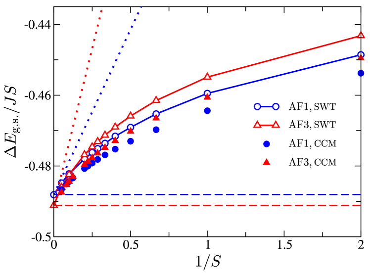
Figure 2: Quantum correction to the ground state energy for the AF1 and AF3 states as a function of inverse spin. Continuous lines with open circles and triangles are the self-consistent spin-wave results. Solid symbols indicate the CCM results. Dashed and dotted lines show the harmonic ($1/S$) and the $(1/S)^{2}$ spin-wave energies.

IV.1 Ground-state properties

We begin with results for the ground-state energies of the two competing antiferromagnetic structures. The harmonic spin-wave theory was used in Ref. 25 to compute the $1/S$ energy correction. An earlier work [5] employed an incorrect magnon spectrum for the collinear AF3 state thus coming to an erroneous conclusion, see [25] for further details. The next order $(1/S)^{2}$ energy correction is straightforwardly obtained using Eq. (II.1) with the harmonic values for $n$, $m_{ij}$, and $\Delta_{ij}$. The first two terms in the $1/S$ series for the ground-state energies of two states are

$$E_{\rm g.s.}^{\rm AF1} = -2JS^{2}\Bigl{[}1+\frac{0.488056}{2S}-\frac{0.186629}{(2S)^{2}}\Bigr{]},$$

$$E_{\rm g.s.}^{\rm AF3} = -2JS^{2}\Bigl{[}1+\frac{0.491106}{2S}-\frac{0.354197}{(2S)^{2}}\Bigr{]}.$$ (32)

The first-order $1/S$ correction lowers the ground-state energy with respect to the classical value $E_{0}=-2JS^{2}$. The corresponding energy shift is larger for the AF3 state but by a very small amount $\Delta E\simeq 0.003JS$.

For frustrated spin models with degenerate classical ground states, an energy gain due to the quantum order by disorder mechanism is typically an order of magnitude larger $0.1$–$0.01JS$. Thus, the harmonic zero-point energies of two collinear magnetic structures in the fcc antiferromagnet appear to be accidentally close to each other. In such a case, higher-order quantum corrections resulting from magnon-magnon interaction can play a decisive role. For the fcc antiferromagnet, the magnon repulsion yields a state-dependent upward shift of the ground-state energies (32). As a result the net energy gain for the AF1 state appears to be larger than for the AF3 structure modifying the conclusion based on the harmonic theory.

The convergence and accuracy of the $1/S$ series are, however, questionable for a frustrated spin model with lines of pseudo-Goldstone (zero-energy) modes. Indeed, the second-order $1/S$ correction to the sublattice magnetization, $\Delta S\simeq\sum_{\bf k}1/\epsilon_{\bf k}^{3}$, diverges for the nearest-neighbor fcc antiferromagnet. To overcome the above problem, we resort to the self-consistent spin-wave calculations described in Sec. II. The renormalized magnon spectrum has only true Goldstone modes and, thus provides a better starting point for computing various physical properties.

The effect of quantum renormalization can be illustrated by comparing bosonic averages in the AF1 ground state for $S=1/2$ obtained self-consistently

$$n=0.14094\,,\ \ m=0.07066\,,\ \ \Delta=0.16381$$ (33)

and from the harmonic spin-wave theory:

$$n=0.33878\,,\ \ m=0.10994\,,\ \ \Delta=0.28537\,.$$ (34)

The interacting spin-wave vacuum is significantly modified in comparison to the noninteracting ground state. In particular, the harmonic theory overestimates $n$ and $\Delta$ by a factor of two. Corresponding values for the AF3 structure are presented in Appendix A.

Figure 2 shows the quantum correction to the classical ground-state energy

$$\Delta E_{\rm g.s.}=E_{\textrm{g.s.}}-E_{0}$$

normalized to $JS$ and plotted as a function of $1/S$. The full lines with open symbols, circles (AF1) and triangles (AF3), indicate energies obtained by the self-consistent spin-wave theory. Numerical CCM results for both states are shown by solid symbols. In addition, the dashed and dotted lines indicate energies calculated to the $1/S$ and the $(1/S)^{2}$ order, respectively.

The total ground-state energies of two collinear states obtained self-consistently for $S=1/2$

$$E_{\rm g.s.}^{\rm AF1}=-0.72425J,\ \ E_{\rm g.s.}^{\rm AF3}=-0.72160J$$ (35)

differ significantly from the first- and the second-order spin-wave results (32). On the other hand, the self-consistent theory and the CCM give remarkably consistent values for $\Delta E_{\rm g.s.}$ as a function of spin. In particular, the CCM ground-state energies in the case of $S=1/2$ are

$$E_{\rm g.s.}^{\rm AF1}=-0.7267(3)J,\ \ E_{\rm g.s.}^{\rm AF3}=-0.7244(3)J,$$ (36)

see Appendix B for further details.

The AF1 state has a lower energy than the AF3 state for all realistic spin values $S<S^{*}\approx 10$. The harmonic-theory prediction is recovered only for unphysically large spins. The remaining difference between spin-wave values and the extrapolated CCM data should be attributed to the magnon scattering processes that are not included in the self-consistent theory.

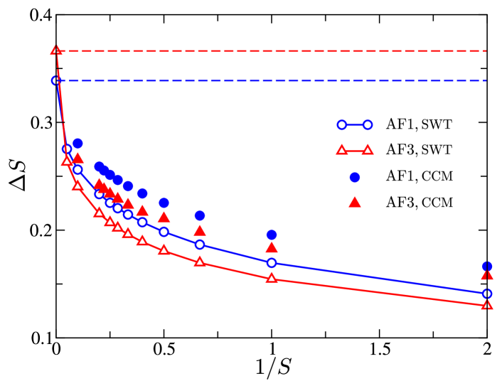
Figure 3: Quantum correction to the sublattice magnetization $\Delta S=S-\langle S\rangle$ in two collinear antiferromagnetic structures. Continuous lines with open circles and triangles are obtained in the self-consistent spin-wave approximation. Solid symbols represent the CCM results. The horizontal dashed lines indicate the harmonic values.

Another effect produced by zero-point fluctuations is reduction of the sublattice magnetization from its classical value $\langle S^{z}\rangle=S$. Figure 3 shows the spin reduction $\Delta S=S-\langle S^{z}\rangle$ obtained in the self-consistent spin-wave approximation and from the extrapolation of the CCM results. The two approaches consistently predict $\Delta S$ to be substantially smaller than the values obtained from the harmonic spin-wave theory. A lack of accuracy of the harmonic approximation can be again related to the presence of spurious pseudo-Goldstone modes in the harmonic magnon spectra, whereas the higher-order quantum corrections restore the correct form of $\epsilon_{\bf k}$, see Sec. IVB below. For $S=1/2$, the ordered moments in the two antiferromagnetic states are reduced by about 30%, which is quite large for a three-dimensional antiferromagnet, but still much smaller than the 70% reduction predicted by the harmonic theory [25].

IV.2 Spectrum renormalization

Quantum fluctuations have a profound effect on the excitation spectra of frustrated magnets with classical ground-state degeneracy. At the harmonic level, degrees of freedom that connect different ground states show up as pseudo-Goldstone modes at zero energy. They are shifted to finite energies by quantum corrections, see, for example, [68, 36, 69, 70]. Below we discuss such renormalization effects focusing on the AF1 state, which is the ground state of the fcc antiferromagnet for all realistic values of spin. Complementary results for the AF3 state are presented in Appendix A.

The collinear AF1 states have a propagation vector at one of the X points in the Brillouin zone, see Fig. 4. Between degenerate antiferromagnetic domains we choose the state described by ${\bf Q}_{1}=(2\pi,0,0)$. The harmonic spectrum of the AF1 state is obtained from general expressions (12) and (13) by keeping terms $O(JS)$ for $A_{\bf k}$ and $B_{\bf k}$. A zero-energy mode appears once the harmonic parameters $A_{\bf k},B_{\bf k}$ obey: (i) $A_{\bf k}=|B_{\bf k}|$ or (ii) $A_{\bf k}=B_{\bf k}=0$. For the fcc antiferromagnet, the pseudo-Goldstone magnons of the first type appear on the lines $(0,q,0)$, $(0,q,2\pi)$, and other equivalent directions in the momentum space. Zero-energy modes of the second type correspond to excitations with the wave vectors $(q,2\pi,0)$ and $(q,0,2\pi)$. Expanding $A_{\bf k},B_{\bf k}$ in the vicinity of these lines, one can straightforwardly show that the magnon energy vanishes linearly $\epsilon_{\bf k}\sim k$ for the type-I modes and quadratically $\epsilon_{\bf k}\sim k^{2}$ for the type-II modes. The top panel of Fig. 4(b) shows the harmonic spectrum of the AF1 state in the plane $k_{y}=2\pi$. The zero-energy modes of two types are present as dark blue valleys of different width that cross at ${\rm X}^{\prime}=(0,2\pi,0)$. Note, that ${\rm X}^{\prime}$ is not the ordering wave vector for the chosen AF1 state.

The above classification of pseudo-Goldstone modes can be extended to a general multisublattice case beyond the simple expression (13) [70]. It is reminiscent of distincting the true Goldstone modes for systems with nonconserved (type-I) and conserved (type-II) order parameters, which represent respectively the usual Heisenberg antiferromagnets and ferromagnets [71]. Once quantum corrections to the spectrum are included within the $1/S$ expansion, the harmonic $A_{\bf k},B_{\bf k}=O(JS)$ receive extra contributions $\delta A_{\bf k},\delta B_{\bf k}=O(J)$. A simple consideration shows that in such a case an energy of a type-I mode increases as $\Delta_{g}=O(JS^{1/2})$, whereas a type-II magnon acquires a smaller gap $\Delta_{g}=O(J)$ [69, 70].

Figures 4(b), 4(c), and 4(d) illustrate quantum renormalization of the magnon spectrum for the AF1 state obtained from the self-consistent spin-wave theory. The false color maps in Fig. 4(b) compare the harmonic and the renormalized spectrum in the $(k_{x},2\pi,k_{z})$ plane for $S=1/2$. Figs. 4(c) and 4(d) show $\epsilon_{\bf k}$ for $S=1/2$ and 5/2, respectively, along a symmetric path in the Brillouin zone indicated in Fig. 4(a). As $S$ increases, the effect of magnon-magnon interaction weakens and, ultimately, the harmonic spectrum should be recovered for $S\to\infty$. Such a tendency is illustrated by considering $\epsilon_{\bf k}$ on the K–$\Gamma$ segment in Figs. 4(c) and 4(d), where magnons have finite energy already in the harmonic approximation.

The segments $\Gamma$–${\rm X}^{\prime}$ and ${\rm X}^{\prime}$–W correspond to the pseudo-Goldstone modes. Magnons along these lines are shifted to finite energies by quantum corrections. For the segment ${\rm X}^{\prime}$–W the energy gap is explicitly given by

$$\Delta_{g}=8J(\Delta-m)\ .$$ (37)

Flat magnon dispersion along this line is accidental and a weak modulation of $\epsilon_{\bf k}$ should arise as a result of higher-order scattering processes excluded in the self-consistent approximation. Note, that the gap obtained by computing the $1/S$ correction to the spectrum has the same form (37) but its value is twice as large as the self-consistent result, cf. Eqs. (33) and (34). Comparing results for $S=1/2$ and $S=5/2$ one can also observe different scaling of magnon energies on the paths $\Gamma$–X^′ and X^′–W, which correspond to type-I and type-II pseudo-Goldstone modes, respectively.

 

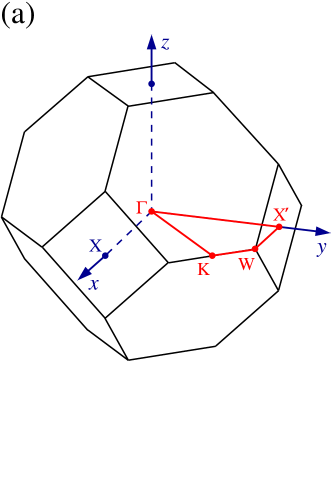
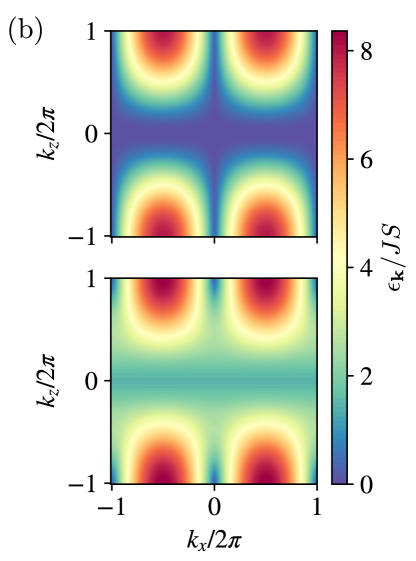
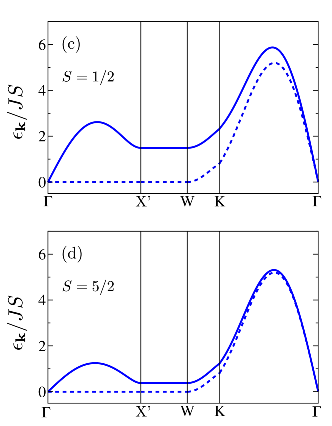
Figure 4: Magnon dispersion in the AF1 state. (a) The Brillouin zone of the fcc lattice with a high-symmetry momentum path. (b) False color plots of $\epsilon_{\bf k}$ within the $k_{y}=2\pi$ plane computed in the harmonic theory (upper panel) and in the self-consistent approximation for $S=1/2$ (lower panel). Spin-wave dispersions along the high-symmetry path for (c) $S=1/2$ and (d) $S=5/2$. Full lines show the results of the self-consistent calculations, dashed lines indicate the harmonic spectra.

Zero-energy modes of the renormalized spectrum correspond to two Goldstone modes at $\Gamma$ and X points. The velocity of acoustic magnons is anisotropic with the two principal values

$$c_{\parallel}=4J(S-n+\Delta),\ \ c_{\perp}=2J\sqrt{2(S-n+\Delta)(\Delta-m)},$$ (38)

where $\parallel$ and $\perp$ are taken with respect to the $\Gamma$–X direction. The dispersion along the $\Gamma$–X line is finite in the harmonic approximation, hence, $c_{\parallel}=O(JS)$. The harmonic spectrum has two orthogonal lines of zero-energy modes in the $y$–$z$ plane and, as a result, the corresponding velocity in the renormalized spectrum is generally smaller $c_{\perp}=O(JS^{1/2})$.

Similar results for the spectrum renormalization were also obtained for the AF3 state. The corresponding plots are presented in Appendix A. Here we summarize the main qualitative features. The majority of pseudo-Goldstone modes for the AF3 state belong to the type I. If we choose for the ordering wave vector of the AF3 state ${\bf Q}_{3}=(2\pi,\pi,0)$, then the only type-II pseudo-Goldstone mode exists at ${\rm X}^{\prime}=(0,2\pi,0)$ and equivalent points. The expression for the quantum gap at this point

$$\Delta_{g}=8J\sqrt{(\Delta_{aa}-m)(\Delta_{ab}-m)}$$ (39)

resembles Eq. (37) for the AF1 state. The anisotropic velocity for the acoustic modes in the AF3 state is given by

$$c_{\parallel} = 2J\sqrt{[2(S-n)+\Delta_{aa}+\Delta_{ab}](\Delta_{ab}-m)}\,,$$

$$c_{\perp} = J\bigl{[}4(S-n)+2\Delta_{aa}+2\Delta_{ab}\bigr{]}^{1/2}$$

$$\mbox{}\times\bigl{[}2(S-n)+2\Delta_{aa}+\Delta_{ab}-m\bigr{]}^{1/2}\,.$$

In contrast to the results for the AF1 state (38), two components of the magnon velocity behave as $c_{\perp}=O(JS)$ and one as $c_{\parallel}=O(JS^{1/2})$.

All the above allows us to conclude that the quantum excitation spectrum in the AF1 state for the large-$S$ fcc antiferromagnet is intrinsically softer than in the AF3 state. This qualitative conclusion has important implication for the low-temperature behavior. In a 3D case, for $T\ll J$, an acoustic mode contributes

$$\Delta F/V=-\frac{\pi^{2}}{90}\,\frac{T^{4}}{c_{\parallel}c_{\perp}^{2}}\ ,$$ (41)

to the free energy per volume. Since $c_{\parallel}c_{\perp}^{2}\simeq S^{2}$ and $S^{5/2}$ for AF1 and AF3 states, respectively, stability of the former state is further enhanced by the thermal fluctuations. At intermediate temperatures $T\sim\Delta_{g}$, magnons with energies above the quantum gap become also excited. Their density of states is obviously larger for the AF1 structure, since the gap (37) is present on the lines, whereas (39) appears only at separate points in the Brillouin zone. Thus, the conclusion that thermal fluctuations favor the AF1 state should hold also in the intermediate temperature range. At higher temperature $T\sim J$, thermal corrections to the spectrum become important and no statement can be made without further studies. Still, we note that the previous harmonic spin-wave analysis [25] as well as the classical Monte Carlo simulations [16] all predict the AF1 state due to the thermal order by disorder suggesting this selection to be a universal result for the fcc antiferromagnet. Hence, the scenario with a finite-temperature transition between the AF3 and AF1 states previously discussed in [25] may be realized for small $J_{2}>0$, which favors at the classical level the AF3 state at $T=0$.

V Conclusions

The problem of long-range ordering for the nearest-neighbor fcc antiferromagnet was raised more than fifty years ago [1, 2, 3, 4, 5]. In our work we give for the first time a comprehensive solution of this problem at $T=0$ using the interacting self-consistent spin-wave theory and the numerical CCM method. We find that the state selection by quantum fluctuations proceeds differently for $S<S^{*}$ and $S>S^{*}$ corresponding, collinear AF1 and AF3 states, respectively. The separation point at $S^{*}\approx 10$ indicates that magnon-magnon interaction plays a significant role for all physical values of spin.

We find good agreement between the two theoretical methods for the ground-state energies and values of ordered moments for the competing collinear states. In addition, the self-consistent spin-wave calculations provide also the magnon spectrum renormalization. The magnon-magnon interaction produces finite quantum gaps for the pseudo-Goldstone modes leaving only two acoustic branches in accordance with the spontaneous breaking of the continuous symmetry in the collinear antiferromagnetic state. The normal form of the magnon spectra explains why the self-consistent spin-wave calculations provide more accurate numerical predictions in comparison with the harmonic theory and the second-order $1/S$ results. Previously the self-consistent spin-wave theory was compared to the numerical results for the $J_{1}$–$J_{2}$ square-lattice antiferromagnet for $J_{2}>0.5J_{1}$ [48]. Our work provides further evidence that the self-consistent approach has good accuracy also for infinitely degenerate frustrated spin models.

The spectacular failure of the harmonic theory to predict the correct ground state as a result of the quantum order by disorder is related to a close proximity $\Delta E\sim 10^{-3}JS$ of the harmonic energies for the two contenders for the ground state. In such a case the higher-order quantum corrections determined by magnon interaction play an important role. The example of the nearest-neighbor fcc antiferromagnet is by no means unique. Another example of a close proximity of the harmonic ground-state energies is realized for the kagome antioferromagnet in a wide range of applied magnetic fields $0.5H_{s}<H<H_{s}$ [72]. Elucidating the state selection due to magnon interaction for this model represent an interesting open theoretical problem.

Aknowledgments

We acknowledge helpful discussions with Y. Iqbal and A. L. Chernyshev. J.R. thanks the Deutsche Forschungsgemeinschaft for financial support (DFG RI 615/25-1). M.E.Z. was supported by ANR, France (Grant No. ANR-18-CE05-0023).

Appendix A Self-consistent theory for the AF3 state

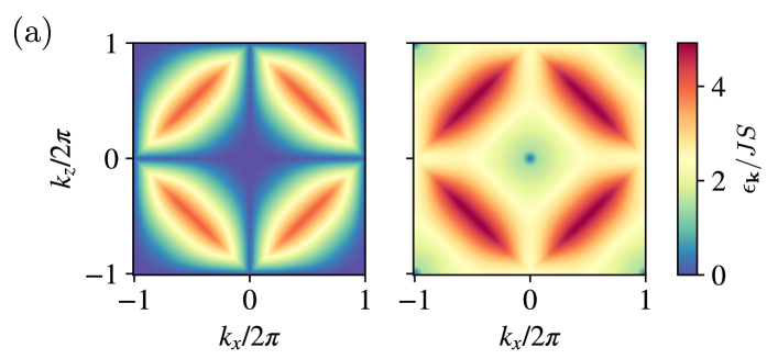
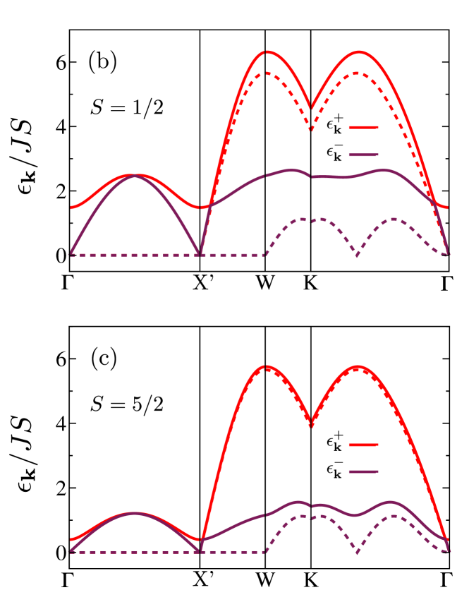
Figure 5: Magnon dispersion in the AF3 state. (a) False color plots of $\epsilon_{\bf k}$ within the $k_{y}=2\pi$ plane computed in the harmonic theory (left panel) and in the self-consistent approximation for $S=1/2$ (right panel). Spin-wave dispersions along the high-symmetry path for (b) $S=1/2$ and (c) $S=5/2$. Full lines show the results of the self-consistent calculations, dashed lines indicate the harmonic spectra.

In this Appendix we provide additional details on the self-consistent spin-wave calculations for the AF3 state. We begin by deriving expressions for the mean-field parameters $n$, $m$, $\Delta_{aa}$, and $\Delta_{ab}$ by a method that avoids an explicit use of the Bogolyubov matrix transformation. The idea consists in adding to the mean-field quadratic Hamiltonian an extra source term linear in a required combination of boson operators. For example, to compute $n=\langle a_{i}^{\dagger}a_{i}\rangle$ we write

$$\hat{\cal H}(h)=\hat{\cal H}^{(2)}_{\rm MF}+h\sum_{i}a_{i}^{\dagger}a_{i}\ .$$ (42)

The Hamiltonian $\hat{\cal H}(h)$ can be straightforwardly diagonalized and the magnon spectrum is given by the same expression (24) with a substitution $S_{0}\to(S_{0}+h/4J)$. The expectation value in the ground state for the considered combination of boson operators is obtained as

$$n=\frac{1}{N}\left.\frac{\partial E_{\textrm{g.s.}}(h)}{\partial h}\right|_{h\rightarrow 0}\ ,$$ (43)

where $N$ is the number of sites. Explicitly,

$$n+\frac{1}{2} = \frac{1}{N}\sum_{\bf k,\pm}\frac{2J}{\epsilon^{\pm}_{\bf k}}\biggl{\{}2S_{0}\pm\frac{S_{m}}{\sqrt{Q_{\bf k}}}\Bigl{[}2S_{0}S_{m}$$ (44)

$$- S_{a}S_{b}c_{x}c_{z}(\gamma_{\bf k}^{2}+\gamma_{\bf k}^{*2})\Bigr{]}\biggr{\}}.$$

Here the momentum summation is performed over the reduced Brillouin zone. Similar calculation for the other averages yields:

$$m = \frac{1}{N}\sum_{\bf k,\pm}\frac{2J}{\epsilon^{\pm}_{\bf k}}\biggl{\{}S_{m}|\gamma_{\bf k}|^{2}\pm\frac{1}{\sqrt{Q_{\bf k}}}\Bigl{[}2S_{0}^{2}S_{m}|\gamma_{\bf k}|^{2}$$

$$- S_{0}S_{a}S_{b}c_{x}c_{z}(\gamma_{\bf k}^{2}+\gamma_{\bf k}^{*2})+\frac{1}{2}S_{m}S_{b}^{2}(\gamma_{\bf k}^{2}-\gamma_{\bf k}^{*2})^{2}\Bigr{]}\biggr{\}},$$

$$\Delta_{aa} = \frac{1}{N}\sum_{\bf k,\pm}\frac{2J}{\epsilon^{\pm}_{\bf k}}\biggl{\{}S_{a}c_{x}^{2}c_{z}^{2}\mp\frac{S_{b}}{\sqrt{Q_{\bf k}}}\Bigl{[}2S_{a}S_{b}c_{x}^{2}c_{z}^{2}|\gamma_{\bf k}|^{2}$$ (45)

$$- S_{0}S_{m}c_{x}c_{z}(\gamma_{\bf k}^{2}+\gamma_{\bf k}^{*2})\Bigr{]}\biggr{\}},$$

$$\Delta_{ab} = \frac{1}{N}\sum_{\bf k,\pm}\frac{2J}{\epsilon^{\pm}_{\bf k}}\biggl{\{}S_{b}|\gamma_{\bf k}|^{2}\mp\frac{1}{\sqrt{Q_{\bf k}}}\Bigl{[}2S_{a}^{2}S_{b}c_{x}^{2}c_{z}^{2}|\gamma_{\bf k}|^{2}$$

$$- S_{0}S_{m}S_{a}c_{x}c_{z}(\gamma_{\bf k}^{2}+\gamma_{\bf k}^{*2})+\frac{1}{2}S_{m}^{2}S_{b}(\gamma_{\bf k}^{2}-\gamma_{\bf k}^{*2})^{2}\Bigr{]}\biggr{\}},$$

The system of four self-consistent equations was solved iteratively. Values for the four parameters in the AF3 ground state for $S=1/2$ are

$$n=0.1297,\ m=0.0578,\ \Delta_{aa}=0.1613,\ \Delta_{ab}=0.1411.$$

Again, a significant renormalization is observed in comparison with the harmonic values

$$n=0.3663,\ m=0.0284,\ \Delta_{aa}=0.2943,\ \Delta_{ab}=0.2232.$$

The magnon dispersion in the AF3 state can be computed using Eq. (24) and self-consistently obtained parameters $n$, $m$, $\Delta_{aa}$, and $\Delta_{ab}$. Results for $\epsilon_{\bf k}$ for fcc antiferromagnets with $S=1/2$ and 5/2 that compliment similar plots for the AF1 state in Sec. IV are included in Fig. 5. We choose a domain of the AF3 state described by ${\bf Q}_{3}=(2\pi,\pi,0)$ as the propagation vector. In our spin-wave description of the AF3 state in Sec. IIC we introduce two (parallel) sublattices. Consequently, we find two different magnon branches and have to consider accordingly the reduced magnetic Brillouin zone shown in Fig. 5(a). Still for the plots in Figs. 5(c) and 5(d) we use a high-symmetry path in the paramagnetic Brillouin zone. Therefore, some wave vectors become equivalent in the reduced Brillouin zone notations. In particular, the ${\rm X}^{\prime}=(0,2\pi,0)$ point is equivalent to the $\Gamma$ point, which explains an extra acoustic mode at ${\rm X}^{\prime}$ present in Figs. 5.

Table 1: CCM results for the ground-state energy per site $E_{\rm g.s.}$ and the sublattice magnetization $\langle S\rangle$ in the AF1 and AF3 states with $S=1/2$ and $S=1$.

$S=1/2$	AF1		AF3
	$E_{\rm g.s.}$	$\langle S\rangle$	$E_{\rm g.s.}$	$\langle S\rangle$
SUB2-2	$-0.69434$	0.42655	$-0.69266$	0.42830
SUB4-4	$-0.71708$	0.39209	$-0.71557$	0.39509
SUB6-6	$-0.72239$	0.37529	$-0.72059$	0.37970
SUB8-8	$-0.72417$	0.36597	$-0.72217$	0.37162
extra 2-6	$-0.72690$	0.33369	$-0.72478$	0.34244
extra 2-8	$-0.72673$	0.33390	$-0.72453$	0.34346
extra 4-8	$-0.72640$	0.33439	$-0.72406$	0.34585

$S=1$	AF1		AF3
	$E_{\rm g.s.}$	$M$	$E_{\rm g.s.}$	$M$
SUB2-2	$-2.40691$	0.90603	$-2.40248$	0.90916
SUB4-4	$-2.44875$	0.86544	$-2.44598$	0.86973
SUB6-6	$-2.45734$	0.84736	$-2.45411$	0.85372
SUB8-8	$-2.45982$	0.83793	$-$	$-$
extra 2-6	$-2.46440$	0.80437	$-2.46063$	0.81739
extra 2-8	$-2.46379$	0.80549	$-$	$-$
extra 4-8	$-2.46262$	0.80807	$-$	$-$

Appendix B CCM results

Extrapolation of numerical results of different SUB$n$-$n$ approximation schemes to $n\to\infty$ was performed using Eq. (31). For $S=1/2$ we have obtained the series with $n=2,4,6,8$ for both antiferromagnetic structures. Accordingly, it is possible to construct three different extrapolations in the $S=1/2$ case that are summarized in the Table. A small spread of final values give an estimate for the error bar on the final result quoted in (36).

For the spin-1 model the $n=2$–8 series was obtained only for the AF1 structure. For the AF3 state with $S=1$, as well as for all $S>1$ we have to rely on the shorter series $n=2,4,6$, which allows only a single extrapolation according to Eq. (31). The numerical results for the $S=1$ case are also included in the Table.

References

- [1] P. W. Anderson, Phys. Rev. 79, 705 (1950).
- [2] J. M. Luttinger, Phys. Rev. 81, 1015 (1951).
- [3] Y.-Y. Li, Phys. Rev. 84, 721 (1951).
- [4] J. M. Ziman, Proc. Phys. Soc. A 66, 89 (1953).
- [5] D. ter Haar and M. E. Lines, Phil. Trans. R. Soc. London A 255, 1 (1962).
- [6] M. E. Lines, Proc. R. Soc. London A 271, 105 (1963).
- [7] M. E. Lines, Phys. Rev. 271, A1336 (1964).
- [8] Y. Yamamoto and T. Nagamiya, J. Phys. Soc. Jpn. 32, 1248 (1972).
- [9] R. H. Swendsen, J. Phys. C 6, 3763 (1973).
- [10] T. Oguchi, H. Nishimori, and T. Taguchi, J. Phys. Soc. Jpn. 54, 4494 (1985).
- [11] C. L. Henley, J. Appl. Phys. 61, 3962 (1987).
- [12] H. T. Diep and H. Kawamura, Phys. Rev. B 40, 7019 (1989).
- [13] M. T. Heinilä and A. S. Oja, Phys. Rev. B 48, 16514 (1993).
- [14] T. Yildirim, A. B. Harris, and E. F. Shender, Phys. Rev. B 58, 3144 (1998).
- [15] K. Lefmann, and C. Rischel, Eur. Phys. J. B 21, 313 (2001).
- [16] M. V. Gvozdikova and M. E. Zhitomirsky, JETP Lett. 81, 236 (2005).
- [17] A. N. Ignatenko, A. A. Katanin, and V. Y. Irkhin, JETP Lett. 87, 555 (2008).
- [18] A. M. Cook, S. Matern, C. Hickey, A. A. Aczel, and A. Paramekanti, Phys. Rev. B 92, 020417 (2015).
- [19] L. A. Batalov and A. V. Syromyatnikov, J. Magn. Magn. Mater. 414, 180 (2016).
- [20] P. Sinkovicz, G. Szirmai, and K. Penc, Phys. Rev. B 93, 075137 (2016).
- [21] F.-Y. Li, Y.-D. Li, Y. Yu, A. Paramekanti, and G. Chen, Phys. Rev. B 95, 085132 (2017).
- [22] A. Singh, S. Mohapatra, T. Ziman, and T. Chatterji, J. Appl. Phys. 121, 073903 (2017).
- [23] N.-N. Sun and H.-Y. Wang, J. Magn. Magn. Mater. 454, 176 (2018).
- [24] P. Balla, Y. Iqbal, and K. Penc Phys. Rev. Research 2, 043278 (2020).
- [25] R. Schick, T. Ziman, and M. E. Zhitomirsky, Phys. Rev. B 102, 220405 (2020).
- [26] D. Kiese, T. Mueller, Y. Iqbal, R. Thomale, and S. Trebst, preprint arXiv:2011.01269.
- [27] G. H. Wannier, Phys. Rev. 79, 357 (1950).
- [28] M. S. Seehra and T. M. Giebultowicz, Phys. Rev. B 38, 11898 (1988).
- [29] M. Matsuura, Y. Endoh, H. Hiraka, K. Yamada, A. S. Mishchenko, N. Nagaosa, and I. V. Solovyev, Phys. Rev. B 68, 094409 (2003).
- [30] A. L. Goodwin, M. T. Dove, M. G. Tucker, and D. A. Keen, Phys. Rev. B 75, 075423 (2007).
- [31] A. A. Aczel, A. M. Cook, T. J. Williams, S. Calder, A. D. Christianson, G.-X. Cao, D. Mandrus, Y.-B. Kim, and A. Paramekanti, Phys. Rev. B 93, 214426 (2016).
- [32] T. Chatterji, L. P. Regnault, S. Ghosh. and A. Singh, J. Phys.: Condens. Matter 31, 125802 (2019).
- [33] N. Khan, D. Prishchenko, Y. Skourski, V. G. Mazurenko, and A. A. Tsirlin, Phys. Rev. B 99, 144425 (2019).
- [34] A. Revelli, C. C. Loo, D. Kiese, P. Becker, T. Frohlich, T. Lorenz, M. Moretti Sala, G. Monaco, F. L. Buessen, J. Attig, M. Hermanns, S. V. Streltsov, D. I. Khomskii, J. van den Brink, M. Braden, P. H. M. van Loosdrecht, S. Trebst, A. Paramekanti, and M. Gruninger, Phys. Rev. B 100, 085139 (2019).
- [35] L. Bhaskaran, A. N. Ponomaryov, J. Wosnitza, N. Khan, A. A. Tsirlin, M. E. Zhitomirsky, and S. A. Zvyagin, Phys. Rev. B 104, 184404 (2021).
- [36] E. F. Shender, Zh. Eksp. Teor. Fiz. 83, 326 (1982) [Sov. Phys. JETP 56, 178 (1982)].
- [37] C. L. Henley, Phys. Rev. Lett. 62, 2056 (1989).
- [38] A. V. Chubukov and D. I. Golosov, J. Phys.: Condens. Matter 3, 69 (1991).
- [39] M. E. Zhitomirsky, J. Phys.: Conf. Ser. 592, 012110 (2015).
- [40] D. C. Johnston, R. J. McQueeney, B. Lake, A. Honecker, M. E. Zhitomirsky, R. Nath, Y. Furukawa, V. P. Antropov, and Y. Singh, Phys. Rev. B 84, 094445 (2011).
- [41] M. Takahashi, Phys. Rev. B 40, 2494 (1989).
- [42] J. H. Xu and C. S. Ting, Phys. Rev. B 42, 6861 (1990).
- [43] A. F. Barabanov and O. A. Starykh, JETP Lett. 51, 312 (1990).
- [44] L. Bergomi and T. Jolicoeur, J. de Phys. I 2, 371 (1992).
- [45] V. Y. Irkhin, A. A. Katanin, and M. I. Katsnelson, J. Phys.: Condens. Matter 4, 5227 (1992).
- [46] I. G. Gochev, Phys. Rev. B 49, 9594 (1994).
- [47] A. V. Dotsenko and O. P. Sushkov, Phys. Rev. B 50, 13821 (1994).
- [48] R. R. P. Singh, W. Zheng, J. Oitmaa, O. P. Sushkov, and C. J. Hamer, Phys. Rev. Lett. 91, 017201 (2003).
- [49] G. S. Uhrig, M. Holt, J. Oitmaa, O. P. Sushkov, and R. R. P. Singh, Phys. Rev. B 79, 092416 (2009).
- [50] J. Takano, H. Tsunetsugu, and M. E. Zhitomirsky, J. Phys.: Confer. Series 320, 012011 (2011).
- [51] A. Werth, P. Kopietz, and O. Tsyplyatyev, Phys. Rev. B 97, 180403(R) (2018).
- [52] S. Yamamoto and Y. Noriki, Phys. Rev. B 99, 094412 (2019).
- [53] T. Holstein and H. Primakoff, Phys. Rev. 58, 1098 (1940).
- [54] R. M. White, M. Sparks, and I. Ortenburger, Phys. Rev. 139, A450 (1965).
- [55] J. H. P. Colpa, Physica A 93, 327 (1978).
- [56] C. Zeng, D. J. J. Farnell, and R. F. Bishop, J. Stat. Phys. 90, 327 (1998).
- [57] R. Darradi, O. Derzhko, R. Zinke, J. Schulenburg, S. E. Krüger and J. Richter, Phys. Rev. B 78, 214415 (2008).
- [58] D. J. J. Farnell, R. Zinke, J. Schulenburg, and J. Richter, J. Phys.: Cond. Matter 21, 406002 (2009).
- [59] O. Götze, D. J. J. Farnell, R. F. Bishop, P. H. Y. Li, and J. Richter, Phys. Rev. B 84, 224428 (2011).
- [60] D. J. J. Farnell, O. Götze, J. Richter, R. F. Bishop, and P. H. Y. Li, Phys. Rev. B 89, 184407 (2014).
- [61] D. J. J. Farnell, O. Götze, and J. Richter, Phys. Rev. B 93, 235123 (2016).
- [62] J.-J. Jiang, F. Tang, and C. H. Yang, J. Phys. Soc. Jpn. 84, 124710 (2015).
- [63] D. J. J. Farnell, O. Götze, J. Schulenburg, R. Zinke, R. F. Bishop, P. H. Y. Li, Phys. Rev. B 98, 224402 (2018)
- [64] R.F. Bishop, P.H.Y. Li, O. Götze, and J. Richter, Phys. Rev. B 100, 024401 (2019).
- [65] J.-J. Jiang, J. Magn. Magn. Mat. 539, 168392 (2021).
- [66] For typically the notation LSUB is used. Note that for the LSUB scheme is identical to the SUB- scheme.
- [67] For the numerical calculation we use the program package ‘The crystallographic CCM’ (D. J. J. Farnell and J. Schulenburg).
- [68] E. Belorizky, R. Casalegno, and J. J. Niez, Phys. Stat. Sol. (b) 102, 365 (1980).
- [69] A. V. Chubukov and T. Jolicoeur, Phys. Rev. B 46, 11137 (1992).
- [70] J. G. Rau, P. A. McClarty, and R. Moessner, Phys. Rev. Lett. 121, 237201 (2018).
- [71] H. Watanabe and H. Murayama, Phys. Rev. Lett. 108, 251602 (2012).
- [72] S. R. Hassan and R. Moessner, Phys. Rev. B 73, 094443 (2006).